


1. Introduction
The incompressible flow of an inviscid liquid with a free surface over topography and/or subject to a surface pressure distribution is a classical problem in fluid dynamics that has received considerable attention over the last two hundred years (see, for example, Whitham Reference Whitham1974; Akylas Reference Akylas1984; Dias & Vanden-Broeck Reference Dias and Vanden-Broeck2002). The principal aim is to determine the free-surface profile and to explore how it changes as the relevant parameters, such as the oncoming flow speed or the amplitude of the forcing (either the topography or pressure distribution), are varied. For a localised forcing, it is well known that in one possible steady flow configuration, herein referred to as a hydraulic fall, the fluid level drops from a higher uniform level upstream to a lower uniform level downstream (figure 1). Such flows have been observed experimentally (e.g. Forbes & Schwartz Reference Forbes and Schwartz1982; Tam et al. Reference Tam, Yu, Kelso and Binder2015), and have been computed as solutions to the fully nonlinear irrotational Euler equations (e.g. Forbes Reference Forbes1988; Dias & Vanden-Broeck Reference Dias and Vanden-Broeck1989), and as solutions to reduced-order models such as the forced Korteweg–de Vries (fKdV) equation (see, for example, Forbes & Schwartz Reference Forbes and Schwartz1982; Dias & Vanden-Broeck Reference Dias and Vanden-Broeck2002). A recent review is provided by Binder (Reference Binder2019).

Figure 1. Hydraulic-fall solutions. Sketch of the two basic types in the non-dimensional domain, where the arrow indicates the flow direction: (a) dip forcing,  $Fr<1$; (b) bump forcing, $Fr<1$. Here, $Fr$ is the Froude number, defined in (1.1). The downstream Froude number, $Fr_{d}$, is of opposite criticality to $Fr$.
$Fr$.
Most of the studies in the literature that concern hydraulic-fall solutions focus on steady flow, and there appears to have been very little effort devoted to gaining a theoretical understanding of the stability of these flows. Experimental studies have tended to concentrate on flow over a bump as depicted in figure 1(b), and, indeed, we have been unable to identify any experimental work on hydraulic falls over a dip (figure 1a). This may simply be due to the fact that presumably a wave tank with a bump is easier to engineer than one with a dip. In this paper, we discuss the stability properties of hydraulic-fall solutions for both positive and negative forcings: (i) by carrying out a linear stability analysis; and (ii) by developing a computational framework based on the finite-element method that we use to analyse nonlinear stability. We show that over a bump, the hydraulic-fall solution is spectrally stable, but over a dip, it is linearly unstable. Most intriguingly, from our suite of time-dependent calculations we identify a new time-dependent invariant solution of the fully nonlinear system that corresponds to a stable time-periodic orbit in a suitably defined phase space.
The fKdV equation and fully nonlinear steady solution spaces for various topographic forcings are by now well established (e.g. Forbes & Schwartz Reference Forbes and Schwartz1982; Dias & Vanden-Broeck Reference Dias and Vanden-Broeck2002; Wade et al. Reference Wade, Binder, Mattner and Denier2014, Reference Wade, Binder, Mattner and Denier2017). For the fKdV system, a number of different solution types can be identified (Akylas Reference Akylas1984; Dias & Vanden-Broeck Reference Dias and Vanden-Broeck2002; Binder, Blyth & McCue Reference Binder, Blyth and McCue2013); for a recent review, see Binder (Reference Binder2019). Broadly speaking, these can be classified as cnoidal wave solutions that are flat upstream and wavy downstream, solitary-wave solutions that are flat both upstream and downstream, and transcritical solutions that we are herein referring to as hydraulic falls. These solutions are characterised by the upstream depth-based Froude number given by
 \begin{equation} Fr = \frac{U}{\sqrt{gH}},\end{equation}
where  $g$ is the gravitational constant, and $U$ and $H$ are the speed of the flow and the fluid depth far upstream. Cnoidal-wave solutions occur when $Fr<1$ (subcritical flow), and solitary-wave solutions occur when $Fr>1$ (supercritical flow). A distinguishing feature of hydraulic-fall solutions is that the flow upstream is subcritical, and the flow downstream is supercritical. For a given topographic forcing, a steady hydraulic-fall solution exists only for a particular value of $Fr$. Furthermore, for hydraulic-fall solutions, if the forcing is negative (a dip), then the wave profile has a local maximum above the forcing, and if the forcing is positive (a bump), then the fluid depth decreases monotonically from upstream to downstream (see figure 1).
Using numerical simulations of the fKdV system carried out for a number of different types of perturbations to the base steady state, Donahue & Shen (Reference Donahue and Shen2010), Chardard et al. (Reference Chardard, Dias, Nyguyen and Vanden-Broeck2011) and Choi & Kim (Reference Choi and Kim2016) all concluded that a hydraulic fall over a positive forcing is stable. Page & Părău (Reference Page and Părău2014) showed via time-dependent calculations, starting from a small wavy Gaussian perturbation, that the hydraulic fall solution appeared to be stable, although they did not track the long-term behaviour. None of these studies attempted a formal linear stability analysis.
The paper proceeds as follows. In § 2, we state the mathematical problem and the weak formulation of the problem that forms the basis of our numerical framework. In § 3.1, we describe briefly the steady bifurcation structure of the fully nonlinear system. We carry out a linear stability analysis in § 3.2, and a nonlinear stability analysis via direct numerical simulations of the fully nonlinear model in § 3.3. Finally, in §§ 3.4 and 4, we discuss our results and consider possible avenues for future research.
2. Problem formulation
We consider inviscid, irrotational, incompressible flow over a bottom topography under the influence of gravity and neglecting surface tension. The general flow scenario is depicted in figure 2. The fluid flows from left to right over a localised topographic structure seen as a positive bump in the figure. In the absence of the topography so that the bottom is flat, or sufficiently far upstream of the obstacle, the flow consists of a uniform stream of strength  $U$ with uniform fluid depth $H$. Our concern is with the generally unsteady disruption that is provoked at the free surface by the topography.
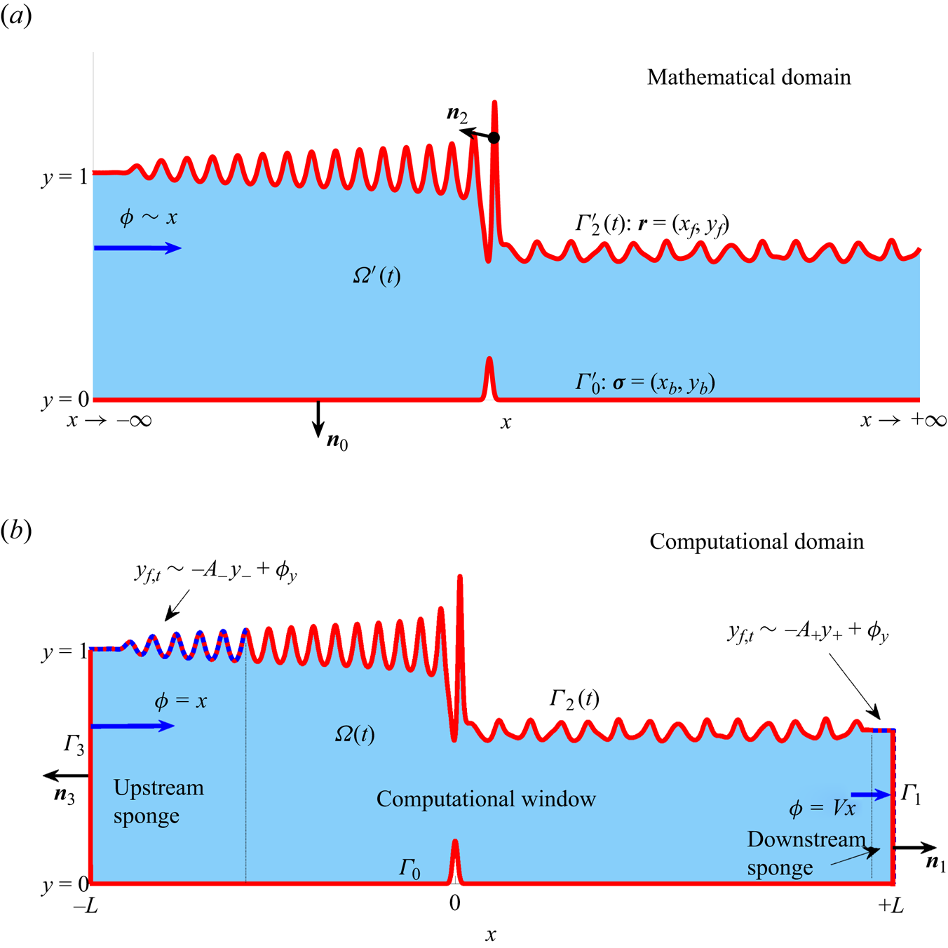
Figure 2. Sketches of the non-dimensional time-dependent problem domain for the hydraulic-fall problem. (a) The mathematical domain. The fluid domain is  $\varOmega '(t)$, the bottom boundary is $\varGamma '_0$, and the free surface is $\varGamma '_2$. As $x\to -\infty$, we impose uniform flow, $\phi \sim x$. (b) The computational domain. The inflow boundary is denoted $\varGamma _3$, and the outflow boundary is $\varGamma _1$. The upstream and downstream sponges are indicated by dotted lines on the free surface $\varGamma _2$. In the computational domain, far downstream we impose that $\phi =Vx$. In both sketches, the normal vectors to each boundary $\varGamma _i$ are given as $\boldsymbol {n}_i$.
We solve for the fluid flow and the deformation of the free surface using a numerical finite-element method. In the following subsections we first describe the mathematical problem to be solved, before discussing the truncated computational problem that is required for the numerical implementation. To aid the discussion, we use primes to denote regions and boundaries in the mathematical problem. For example,  $\varOmega '(t)$ represents the fluid domain in the mathematical problem, and $\varOmega (t)$ represents the corresponding truncated computational domain.
2.1. Mathematical formulation
We non-dimensionalise the problem by scaling all lengths and velocities by the height  $H$ and strength $U$ of the oncoming uniform stream, respectively. The corresponding time scale is $H/U$. Figure 2(a) shows the domain for the mathematical problem expressed in terms of dimensionless variables and with reference to a Cartesian set of axes $\boldsymbol {x} = (x,y)$. The free surface is described by $\boldsymbol {r}= (x_f(s,t),y_f(s,t))$, and the bottom topography by $\boldsymbol {\sigma } = (x_b(s),y_b(s))$, where $s$ is a suitably chosen parameter (e.g. arc length). Written in terms of the velocity potential $\phi (\boldsymbol {x},t)$, the dimensionless governing equation and boundary conditions are
 $$\begin{gather} \nabla^2\phi = 0,\quad \boldsymbol{x}\in\varOmega'(t)\quad (\text{conservation of mass}), \end{gather}$$
 $$\begin{gather}\boldsymbol{\nabla}\phi\boldsymbol{\cdot}\boldsymbol{n}_0 = 0,\quad \boldsymbol{x}\in\varGamma'_0,\quad (\text{no penetration on bottom}), \end{gather}$$
 $$\begin{gather}\frac{\partial \boldsymbol{r}}{\partial t}\boldsymbol{\cdot} \boldsymbol{n}_2 = \boldsymbol{\nabla}\phi\boldsymbol{\cdot} \boldsymbol{n}_2 ,\quad \boldsymbol{x}\in\varGamma'_2(t) \quad (\text{kinematic condition}), \end{gather}$$
 $$\begin{gather}\phi_t + \frac{1}{2}\,|\boldsymbol{\nabla}\phi|^2 + \frac{1}{Fr^2}\,(y_f-1) - \frac{1}{2} = 0,\quad \boldsymbol{x}\in\varGamma'_2(t)\quad (\text{dynamic condition}). \end{gather}$$
The Froude number  $Fr$ was defined in (1.1). The dynamic boundary condition follows from applying Bernoulli's equation at the free surface and utilising the upstream uniform flow conditions, namely
 \begin{equation} y_f\to 1,\quad \phi \to x \quad \text{as } x\to-\infty.\end{equation}
Throughout, we will adopt the Gaussian topographic forcing function
 \begin{equation} y_b = a\,\text{e}^{{-}b^2x_b^2},\end{equation}
for some  $a,b\in \mathbb {R}$.
2.2. Truncated computational formulation
To prepare for the numerical discretisation, as shown in figure 2(b) we truncate the infinite domain so that  ${x}\in [-L,L]$, with $L$ to be chosen to be sufficiently large. The problem on the truncated domain is given by (2.1)–(2.4) (with the primes on the flow domain and boundary symbols removed). Boundary conditions must be imposed at the artificial outflow and inflow boundaries $\varGamma _1$ and $\varGamma _3$, respectively, that arise due to the truncation.
At the inflow boundary  $\varGamma _3$, corresponding to ${x}=-L$, the velocity potential and free surface level are set to mirror the condition (2.5) in the mathematical formulation. Accordingly, we impose
 \begin{equation} {y}_f = 1,\quad {\phi} = {x}, \quad {\boldsymbol{x}}\in\varGamma_3 \quad (\text{inflow condition}), \end{equation}
which imposes a Dirichlet condition on  $\phi$. The conditions to be imposed at the outflow boundary are more subtle. Anticipating the presence of waves propagating downstream, for our unsteady calculations, we will make use of a sponge layer to force the free surface to become locally flat downstream, allowing us to impose the outflow Neumann boundary condition
 \begin{equation} \boldsymbol{\nabla} {\phi}\boldsymbol{\cdot} \boldsymbol{n}_1 = V \quad \text{on } \boldsymbol{x}\in\varGamma_1\quad (\text{outflow condition}), \end{equation}
where  $\boldsymbol {n}_1=\boldsymbol {i}$ is the unit vector in the $x$ direction, and $V$ is set to ensure conservation of mass. In this way, we expect to capture the genuine flow features across the main part of the computational domain (the ‘computational window’ – see figure 2b), except in a short region close to the outflow and inflow boundaries where the flow is artificially forced into becoming a locally uniform stream. The choice of $V$ together with details of the sponge layer will be discussed below.
2.3. Steady calculations
In presenting the steady solution space we include both types of transcritical flow (hydraulic falls and rises) for completeness and to provide greater context. Since hydraulic-rise solutions are subcritical at the downstream end (contrast the hydraulic fall solutions sketched in figure 1), we found that in practice it is convenient to replace the conditions on  $\phi$ in (2.7) and (2.8) with a Neumann condition on $\phi$ at the inflow boundary $\varGamma _3$, and a Dirichlet condition on $\phi$ at the outflow boundary. In this way, we can prevent the occurrence of cnoidal waves downstream.
As was mentioned above, the downstream speed  $V$ in (2.8) is chosen to ensure conservation of mass. If $\gamma _s = y_f(x=L)$ is the a priori unknown free-surface level local to $\varGamma _1$, then we must choose $V=1/\gamma _s$. The steady form of the dynamic boundary condition (2.4) then requires
 \begin{equation} \frac{1}{2}\,\gamma_s^{{-}2} + \frac{1}{Fr^2}\,(\gamma_s - 1) - \frac{1}{2} = 0. \end{equation}
This is satisfied for any  $Fr$ if $\gamma _s=1$, but if $\gamma _s\neq 1$, then it imposes a constraint on the Froude number, thus the Froude number must come as part of the solution.
While our focus in this paper is on hydraulic-fall solutions, we can also calculate hydraulic-rise solutions for which the fluid depth increases monotonically from its upstream level, where  $Fr>1$, to its downstream level, where $Fr<1$. These solutions are not observed in experiments, so the main focus of our stability analysis is hydraulic falls, although we do present a brief description of the nonlinear stability of hydraulic rises for completeness.
2.4. Time-dependent calculations
In the time-dependent problem when waves reach the artificial boundaries in the truncated computational domain at  $x=\pm L$, either they will be reflected back into the domain, or the simulation will fail. A number of different approaches have been proposed for dealing with this issue (see Romate (Reference Romate1991) for a review). These include imposing appropriate radiation conditions (Buttle et al. Reference Buttle, Pethiyagoda, Moroney and McCue2018; Ţugulan, Trichtchenko & Părău Reference Ţugulan, Trichtchenko and Părău2022) or introducing perfectly-matched layers (see, for example, Bermúdez et al. (Reference Bermúdez, Hervella-Nieto, Prieto and Rodrı2007) for acoustic waves). We choose a simpler approach by introducing so-called sponge layers adjacent to the inflow and outflow boundaries. The sponge layer was described by Boyd (Reference Boyd2000) and Alias (Reference Alias2014), and it has been implemented, for example, by Grimshaw & Maleewong (Reference Grimshaw and Maleewong2016) and Keeler, Binder & Blyth (Reference Keeler, Binder and Blyth2017) in the case of the fKdV equation.
In the sponge layers, disturbances near to the inflow and outflow boundaries are exponentially damped, so
 \begin{equation} y_f - y_{{\pm}}\propto \text{e}^{{-}A_{{\pm}}t},\end{equation}
where  $y_-$ and $y_+$ are, respectively, target upstream and downstream free-surface levels that will be discussed below, and $A_+$ and $A_-$ are specified decay rate constants. To achieve this, we modify the kinematic condition (2.3) to become
 \begin{equation} \frac{\partial \boldsymbol{r}}{\partial t}\boldsymbol{\cdot} \boldsymbol{n}_2 - \underbrace{S_-(x)(y_f - y_-)}_{{upstream\ sponge}} - \underbrace{S_+(x)\,(y_f - y_+)}_{{downstream\ sponge}} = \boldsymbol{\nabla} \phi\boldsymbol{\cdot} \boldsymbol{n}_2. \end{equation}
The sponge functions  $S_{\pm }(x)$ take the form
 \begin{align} S_+(x) = A_+[1+\tanh(B_+(x - C_+))],\quad S_{-}(x) = A_-[1 + \tanh({-}B_-(x - C_-))], \end{align}
so that the exponential damping occurs only over specified regions dictated by the parameters  $B_{\pm }$ and $C_{\pm }$. Care must be exercised when choosing values for $A_{\pm },B_{\pm },C_{\pm }$ to ensure that free-surface waves do not get reflected back into the main part of the computational domain. After extensive experimentation, we found that taking $A_{\pm }=5$ is appropriate, setting $B_+ = 1$ ensures that small-amplitude waves are absorbed downstream, and taking $B_-= 0.01$ avoids large-amplitude waves being reflected back into the domain at the upstream end. We set the locations of the sponge layers by taking $C_{\pm } = \pm L \mp 10$, and typically we choose $L>100$ – see figure 2(b), where the sponge region is marked approximately by dashed lines on $\varGamma _2$.
The upstream target level we set as  $y_{-} = 1$, whereas for the downstream target level, we set either $y_+ = \gamma _s$ or $y_+ = 1$, depending on the initial condition. This choice will be discussed in §§ 3.3 and 3.4. Regardless of the choice of $\gamma _s$, we fix $V=1/y_f(L,t)$ so that the outflow flux is equal to unity. We stress that this technique of damping the waves upstream and downstream is independent of the underlying numerical discretisation of the system. It could in principle be applied to the analogous three-dimensional problem as an alternative to the radiation conditions used in Buttle et al. (Reference Buttle, Pethiyagoda, Moroney and McCue2018) and Ţugulan et al. (Reference Ţugulan, Trichtchenko and Părău2022).
2.5. Weak formulation
The governing equations (2.1)–(2.4) are highly nonlinear, and numerical methods are typically required to solve them. Boundary-integral methods are popular (see, for example, Forbes & Schwartz Reference Forbes and Schwartz1982; Dias & Vanden-Broeck Reference Dias and Vanden-Broeck2002; Binder, Vanden-Broeck & Dias Reference Binder, Vanden-Broeck and Dias2005; Binder, Dias & Vanden-Broeck Reference Binder, Dias and Vanden-Broeck2008; Wade et al. Reference Wade, Binder, Mattner and Denier2014, Reference Wade, Binder, Mattner and Denier2017), although finite-difference schemes have been used (Grimshaw, Zhang & Chow Reference Grimshaw, Zhang and Chow2007), and more recently a spectral method has been implemented (Forbes, Walters & Hocking Reference Forbes, Walters and Hocking2021). We choose a different approach and develop a numerical framework based on a weak formulation of the governing equations over the computational domain (figure 2b). The advantages of this approach will be discussed in § 2.6, but first we describe the mathematical weak formulation.
We multiply (2.1) by a test function  $\psi (\boldsymbol {x})$ that is required to vanish on boundaries where Dirichlet conditions in $\phi$ are imposed, for example, $\varGamma _3$. Integrating (2.1) over the computational domain and integrating by parts yields
 \begin{equation} \iint_{\varOmega(t)} (\nabla^2\phi) \psi\,\text{d}V \equiv \int_{\partial\varOmega(t)} (\boldsymbol{n}\boldsymbol{\cdot} \boldsymbol{\nabla} \phi)\psi\,\text{d}S - \iint_{\varOmega(t)} \boldsymbol{\nabla} \phi\boldsymbol{\cdot} \boldsymbol{\nabla} \psi\,\text{d}V = 0,\end{equation}
where  $\partial \varOmega (t)$ represents the boundary of $\varOmega (t)$, $\boldsymbol {n}$ is the outward-pointing unit normal vector on each part of the boundary, and $\text {d}V, \text {d}S$ are differential area and line elements, respectively. The domain boundary can be decomposed into $\partial \varOmega (t) = \varGamma _0 + \varGamma _1 + \varGamma _2(t) + \varGamma _3$, so imposing the Neumann conditions (2.2), (2.3) and (2.8) means that (2.13) becomes
 \begin{align} \mathcal{R}_{Bulk}(\boldsymbol{x},\phi(\boldsymbol{x})) &\equiv \int_{\varGamma_2(t)}\underbrace{\left(\frac{\partial \boldsymbol{r}}{\partial t}\boldsymbol{\cdot} \boldsymbol{n}_2\right)}_{{kinematiccond.}}\psi\,\text{d}S + \int_{\varGamma_1}\underbrace{V}_{{outflow}}\psi\,\text{d}S\nonumber\\ &\quad -\iint_{\varOmega(t)} \boldsymbol{\nabla} \phi\boldsymbol{\cdot} \boldsymbol{\nabla} \psi\,\text{d}V = 0, \end{align}
with the unit normal  $\boldsymbol {n}_2$ identified in figure 2. To satisfy the dynamic boundary condition, we multiply (2.4) by a test function and integrate over the free surface to obtain
 \begin{equation} \mathcal{R}_{Dyn}(\boldsymbol{x},\phi(\boldsymbol{x}))\equiv \int_{\varGamma_2(t)}\left(\phi_t + \frac{1}{2}\,|\boldsymbol{\nabla} \phi|^2 + \frac{1}{Fr^2}\,(y_f-1) - \frac{1}{2}\right)\psi\,\text{d}S = 0.\end{equation}
This finalises the weak formulation of the problem. Equations (2.14) and (2.15) are to be solved to determine the free-surface location  $y_f(x,t)$ and the velocity potential in the fluid $\phi (\boldsymbol {x},t)$.
2.6. Numerical discretisation
To solve (2.14) and (2.15) numerically, we utilise the open-source C++ package oomph-lib (Heil & Hazel Reference Heil and Hazel2006) that discretises the governing equations using a Galerkin finite-element method and allows us to take advantage of state-of-the-art linear solvers and mesh-update techniques, and provides flexibility to switch between steady, time-dependent and linear stability calculations. We utilise an isoparametric representation, wherein the same interpolating shape functions are used for  $\psi$ and for the position variables. For this problem, we used piecewise-cubic shape functions, and typically chose $400 \times 10$ elements in the $x\times y$ directions, which corresponds to $1201\times 31$ nodes. The variation of flow quantities in the $y$ direction is found to be small compared to that in the $x$ direction. It is therefore possible to use a smaller number of elements in the vertical direction. We use a structured quadrilateral mesh with either a spine-node update strategy (for the stability analysis and time-dependent calculations) or a pseudo-solid elastic mesh update strategy (for the steady calculations), although in principle other mesh geometries, such as an unstructured triangular mesh, can be used. Newton iterations are used to calculate steady states and a backwards-difference Euler order 2 implicit method is used for unsteady time-stepping; after extensive experimentation, we set the time step $\Delta t = 1.0$, which is small enough to resolve the temporal features of the solutions to be discussed. An attractive feature of this formulation is that time-dependent calculations require only a very minor (and easy) augmentation of the Jacobian matrix used in the Newton iterations, so it is straightforward to switch between steady-state calculations and time-dependent calculations. Another notable feature is that despite calculating quantities in the bulk fluid as well as the free surface, the corresponding Jacobian matrix is sparse, in contrast to the boundary-integral approaches, and the linear inversion is quick based on the open-source SuperLU package (Li Reference Li2005), which performs LU factorisation. Using $400\times 10$ elements (approximately $30\,000$ unknowns), and working on a standard laptop using a single i7 processor, we find that converging Newton iterations take approximately 13 s for the steady calculations, and for the unsteady calculations, advancing one non-dimensional unit of time takes approximately 8 s. For $400\times 1$ elements (approximately $6000$ unknowns), the aforementioned components of the steady and time-dependent calculations each take approximately 0.2 s.
Finally, in the weak formulation, the numerical generalised eigenvalue problem that results from the linear stability analysis is highly rank deficient as time derivatives do not appear explicitly in the bulk fluid. To compute the eigenvalues and eigenmodes accurately and efficiently, we implement the eigensolver from the Anasazi linear algebra library (Heroux et al. Reference Heroux2003) that is based on Arnoldi iteration and has been used successfully in other rank-deficient generalised eigenproblems (Thompson, Juel & Hazel Reference Thompson, Juel and Hazel2014; Keeler et al. Reference Keeler, Thompson, Lemoult, Juel and Hazel2019).
3. Steady solutions, stability analysis and time-dependent simulations
In this section, we first describe the steady hydraulic-fall solution structure. Next, we establish the linear stability properties of the hydraulic-fall solutions by solving a generalised eigenvalue problem, and probe the nonlinear stability properties by performing time-dependent simulations.
3.1. Steady bifurcation structure
We briefly describe the steady bifurcation structure for the fully nonlinear system. In figure 3, we show the hydraulic-fall solution space in the  $(a,Fr)$ plane (we remind the reader that $a$ is the amplitude of the forcing). The hydraulic-rise steady states are included for completeness.
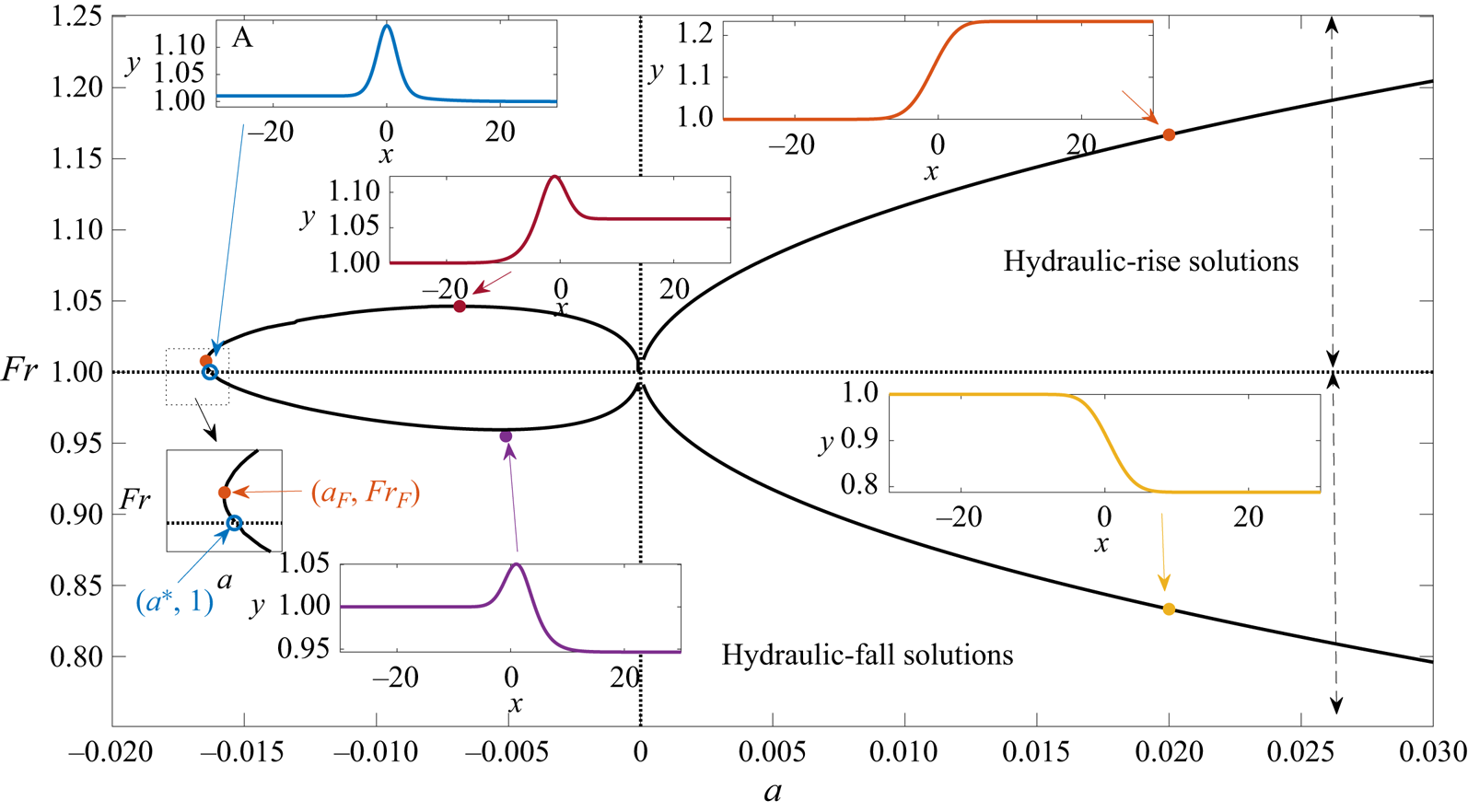
Figure 3. Steady solution space for  $b = 0.3$. The amplitude of the forcing, $a$, is the horizontal measure, and the vertical measure is the Froude number $Fr$. The insets show profiles on the branches indicated by arrows. Here, $a^*\approx -0.016$ and $(a_F, Fr_F) \approx (-0.0165,1.006)$.
We focus on the difference between the free-surface profiles for  $a<0$ and $a>0$. For $a>0$, the hydraulic-fall/rise profiles are monotonic decreasing/increasing functions of $x$, respectively, and there is a unique hydraulic-fall solution for each $a$. For $a<0$, the profiles are non-monotonic, and in each case the wave height reaches a maximum close to $x=0$ before decreasing monotonically (vice versa for the hydraulic-rise profiles).
Unlike the corresponding curve for the fKdV equation with delta function forcing (see, for example, Binder Reference Binder2019), the solution curve in figure 3 is symmetric neither about  $a=0$ nor about $Fr=1$. (Although the latter appears true, close inspection reveals this not to be the case – see the zoomed inset diagram in the figure.) Again in contrast to what is observed for the fKdV equation, the solution curve has a turning point that is located at $(a_F,Fr_F)$, with $Fr_F>1$, so that there is a parameter window $a_F< a < a^*$ in which there is a multiplicity of hydraulic-rise solutions.
There are no hydraulic-fall solutions for  $a \leq a^*$. We encounter numerical difficulties in reaching the point $a=a^*$. As the branch approaches this point, the wave profile, as shown in the top left inset of figure 3 (labelled A) appears to approach a solitary-wave type solution in which the downstream height satisfies $\gamma _s\to 1$. We believe that the profile at $a=a^*$ corresponds to that at the termination point of the $Fr=1$ branch of solution (not computed here), as described by Keeler, Blyth & King (Reference Keeler, Blyth and King2021) for the fKdV model.
3.2. Linear stability analysis
To analyse the stability of the steady solutions discussed in the previous subsection, we first introduce the velocity potential on the free surface,  $\varphi (x,t) \equiv \phi (x,y_f,t)$, and the surface elevation $\eta \equiv y_f - 1$. We then write
 \begin{equation} \varphi = \varphi_s(x) + \hat{\varphi}(x,t),\quad \eta = \eta_s(x) + \hat{\eta}(x,t), \end{equation}
where  $\varphi _s(x)$ and $\eta _s(x)$ are the velocity potential and elevation for a steady hydraulic-fall solution, and the hatted variables are time-dependent perturbations that are assumed to vanish as $x\to \pm \infty$. We emphasise that the perturbations are arbitrary and not at this point assumed to be small.
It is helpful for the subsequent linear stability analysis to write the system of equations in Hamiltonian form. However, since we perturb about steady hydraulic-fall solutions for which the surface potential and elevation functions  $\varphi _s$ and $\eta _s$ do not vanish as $x\to \infty$, some modification to the well-known Craig–Sulem–Zakharov (CSZ) Hamiltonian formulation of the water wave problem (Zakharov Reference Zakharov1968; Craig & Sulem Reference Craig and Sulem1993) is necessary, which we now describe. We note that the base state in (3.1a,b) does not necessarily have to represent a hydraulic-fall solution; the following analysis is also valid if the underlying steady state is a hydraulic-rise or solitary-wave solution, for example.
In constructing the Hamiltonian, it is important to realise that (3.1a,b) reflects a nonlinear perturbation to free-surface quantities, and that some care must be exercised when defining corresponding bulk velocity potentials. In particular, we define  $\xi (x,y,t)$ and $\hat {\phi }(x,y,t)$ to be the solutions to the following Dirichlet–Neumann problems, denoted A and B, which are both defined on the time-dependent domain $\varOmega '(t)$:
 \begin{equation} \text{problem A}\left\{ \begin{array}{@{}l}
\nabla^2 \xi = 0\quad \text{in } \varOmega'(t),\\ \xi =
\varphi_s\quad \text{on } \varGamma'_2(t),\\
\boldsymbol{n}_0\boldsymbol{\cdot} \boldsymbol{\nabla} \xi
= 0\quad \text{on } \varGamma'_0,\\ \xi \sim x \quad
\text{as } x \to -\infty,\\ \xi \sim \gamma_s^{{-}1}x \quad
\text{as } x \to \infty,\\ \end{array} \right. \quad
\text{problem B}\left\{
\begin{array}{@{}l} \nabla^2 \hat{\phi} = 0\quad \text{in }
\varOmega'(t),\\ \hat{\phi} = \hat{\varphi}\quad \text{on }
\varGamma'_2(t), \\ \boldsymbol{n}_0\boldsymbol{\cdot}
\boldsymbol{\nabla} \hat{\phi} = 0\quad \text{on }
\varGamma'_0, \\ \hat{\phi} \to 0 \quad \text{as } x \to
-\infty, \\ \hat{\phi} \to 0 \quad \text{as } x \to \infty.
\end{array}\right. \end{equation}
\begin{equation} \text{problem A}\left\{ \begin{array}{@{}l}
\nabla^2 \xi = 0\quad \text{in } \varOmega'(t),\\ \xi =
\varphi_s\quad \text{on } \varGamma'_2(t),\\
\boldsymbol{n}_0\boldsymbol{\cdot} \boldsymbol{\nabla} \xi
= 0\quad \text{on } \varGamma'_0,\\ \xi \sim x \quad
\text{as } x \to -\infty,\\ \xi \sim \gamma_s^{{-}1}x \quad
\text{as } x \to \infty,\\ \end{array} \right. \quad
\text{problem B}\left\{
\begin{array}{@{}l} \nabla^2 \hat{\phi} = 0\quad \text{in }
\varOmega'(t),\\ \hat{\phi} = \hat{\varphi}\quad \text{on }
\varGamma'_2(t), \\ \boldsymbol{n}_0\boldsymbol{\cdot}
\boldsymbol{\nabla} \hat{\phi} = 0\quad \text{on }
\varGamma'_0, \\ \hat{\phi} \to 0 \quad \text{as } x \to
-\infty, \\ \hat{\phi} \to 0 \quad \text{as } x \to \infty.
\end{array}\right. \end{equation}
We assume that  $\hat {\eta }$ and higher-order corrections to $\xi$ decay sufficiently fast as $x\to \pm \infty$ for the integrals that we will state below (e.g. (3.4)) to be convergent. A subtle point to note is that $\xi$ does not correspond to the velocity potential of the steady state as it is defined on the time-dependent domain, which in general does not coincide with that for the steady state. However, the trace of $\xi$ on the free surface coincides with that for the steady problem. (We note that this construction relies on the assumption that the free surface is a graph.)
The combined velocity potential  $\phi = \xi + \hat {\phi }$ satisfies Laplace's equation (2.1) in the time-dependent domain. Taking inspiration from the CSZ construction, problems A and B have been formulated in such a way that we may write down a Hamiltonian for our problem in the form
 \begin{align} \hat{\mathcal{H}}(\hat{\varphi},\hat{\eta}) &= \hat{\mathcal{H}}_{0}(\xi,\eta_s,\hat{\eta}) + \underbrace{\frac{1}{2}\iint_{\varOmega'(t)} |\boldsymbol{\nabla} \hat{\phi}|^2\,\text{d}V + \frac{1}{2\,Fr^2}\int_{-\infty}^{\infty}\hat{\eta}^2\,\text{d}\kern0.7pt x}_{CSZ}\nonumber\\ &\quad +\underbrace{\iint_{\varOmega'(t)}\boldsymbol{\nabla} \xi\boldsymbol{\cdot} \boldsymbol{\nabla} \hat{\phi}\,\text{d}V +\frac{1}{Fr^2}\int_{-\infty}^{\infty}\eta_{s}\hat{\eta}\,\text{d}\kern0.7pt x}_{{perturbation}}. \end{align}
We have split  $\hat {\mathcal {H}}$ into a term that replicates the original CSZ Hamiltonian, a perturbation term that arises from the nonlinear perturbation in (3.1a,b), and a term that can be considered as the ‘base’ energy, $\hat {\mathcal {H}}_0$, defined as
 \begin{align} \hat{\mathcal{H}}_{0}(\xi,\eta_s,\hat{\eta}) = \int_{-\infty}^{\infty}\left[\frac{1}{2}\int_{0}^{1+\eta_s+\hat{\eta}}(|\boldsymbol{\nabla} \xi|^2 - 1)\,\text{d}y + \frac{1}{2\,Fr^2}\,\eta_s^2 + Q\right]\,\text{d}\kern0.7pt x,\quad Q = \frac{1}{2\,Fr^2}\,\eta_s(\eta_s + 2).\end{align}
It is important to note that the integral in (3.4) is convergent due to the addition of the term  $Q$. (Since $Q$ does not depend on $\hat \phi$ or $\hat \eta$, it does not contribute on taking variations of $\hat {\mathcal {H}}$ with respect to these variables.) As $x\to -\infty$, the terms inside the square brackets in (3.4) vanish due to the inflow conditions (2.7). As $x\to \infty$, they vanish due to the downstream condition (2.9), imposed on the mathematical domain as $x\to \infty$, assuming that we restrict the flow to approach a uniform stream with free-surface height either 1 or $\gamma _s$. This restriction as $x\to \infty$ is satisfied when discussing computations for nonlinear stability in § 3.3.
Finally, by using variational arguments as described in Zakharov (Reference Zakharov1968) and Craig & Sulem (Reference Craig and Sulem1993), it can be shown that the system in (2.1)–(2.4), together with (3.1a,b), can be written as
 \begin{equation} \frac{\partial\boldsymbol{\zeta}}{\partial t} = \boldsymbol{K}\, \frac{\delta\hat{\mathcal{H}}}{\delta{\boldsymbol{\zeta}}},\quad \boldsymbol{K} = \begin{pmatrix} 0 & I\\ -I & 0 \end{pmatrix}, \quad \frac{\delta}{\delta\boldsymbol{\zeta}} = \left(\frac{\delta}{\delta\hat{\eta}},\frac{\delta}{\delta \hat{\varphi}}\right)^{\rm T},\end{equation}
where  $\boldsymbol {\zeta } = (\hat {\eta },\hat {\varphi })^{\rm T}$, and $\delta /\delta \boldsymbol {\zeta }$ is the variational derivative.
Although the stability theory of Hamiltonian systems is well known (see, for example, Holm et al. Reference Holm, Marsden, Ratiu and Weinstein1985), it is helpful to repeat the salient details. First, we linearise (3.5a–c) about  $\hat {\varphi }\equiv 0 \equiv \hat {\eta }$, that is, we set $\boldsymbol {\zeta } = \varepsilon \bar {\boldsymbol {\zeta }}$, with $0<\varepsilon \ll 1$ and $\bar {\boldsymbol {\zeta }} = (\bar {\eta },\bar {\varphi })^{\rm T}$. At $O(\varepsilon )$, we find
 \begin{equation} \frac{\partial \bar{\boldsymbol{\zeta}}}{\partial t} = \boldsymbol{K}\boldsymbol{L} \bar{\boldsymbol{\zeta}}, \quad \boldsymbol{L} = \frac{1}{2}\,\frac{\delta}{\delta\bar{\boldsymbol{\zeta}}}(\delta^2 \hat{\mathcal{H}}),\end{equation}
where  $\delta ^2\hat {\mathcal {H}}$ is the symmetric Hessian matrix (see, for example, Holm et al. Reference Holm, Marsden, Ratiu and Weinstein1985). Proceeding further, we write $\bar {\boldsymbol {\zeta }} = \boldsymbol {g}_s\,\text {e}^{st}$, where $\boldsymbol {g}_s = (g_{\hat {\eta },s}(x),g_{\hat {\varphi },s}(x))^{\rm T}$ so that (3.6a–c) becomes the eigenvalue problem
 \begin{equation} s\boldsymbol{g}_s = \boldsymbol{K}\boldsymbol{L} \boldsymbol{g}_s,\end{equation}
for eigenvalues  $s$ and eigenmodes $\boldsymbol {g}_s$.
We distinguish between two classes of solutions to (3.7), which correspond to (i) a continuous essential spectrum  $s_{ess}$, and (ii) a discrete point spectrum $s_{p}$. The eigenmodes of $s_{ess}$ are bounded as $|x|\to \infty$, whilst the eigenmodes of $s_{p}$ decay to zero as $|x|\to \infty$. With $\boldsymbol {K}$ skew-symmetric and assuming $\boldsymbol {L}$ self-adjoint, it is easy to show that if $s=\rho \in \mathbb {C}$ satisfies (3.7), then so do $s=-\rho$ and $s=\pm \rho ^*$ (where stars indicate complex conjugates), therefore there is a fourfold symmetry in the complex plane. This is a standard distinguishing feature of Hamiltonian systems (see, for example, Holm et al. Reference Holm, Marsden, Ratiu and Weinstein1985).
We calculate  $s_{ess}$ and $s_{p}$ numerically using our finite-element framework (this implementation is identical to the procedure described in Thompson et al. Reference Thompson, Juel and Hazel2014). The calculation is delicate and requires care to ensure convergence. In addition, we remark that to calculate $s_{ess}$ and $s_{p}$, we have to solve three separate numerical problems (one for $s_{ess}$, and two for $s_{p}$); the precise details will be discussed in parallel with the results below.
3.2.1. The essential spectrum  $s_{ess}$

The essential spectrum  $s_{ess}$ can be calculated by examining the form of (3.7) in the limit as $|x|\to \infty$ (see, for example, Sandstede & Scheel Reference Sandstede and Scheel2000). An interesting aspect of this problem is that the operator $\boldsymbol {L}$ takes different forms as $x\to -\infty$ and as $x\to \infty$, and consequently different dispersion relations are obtained in these limits. This has implications for the spatial wavenumber of the eigenmodes.
Sufficiently far downstream, the flow corresponds to a uniform stream of height  $\gamma _s$ with speed $V = \gamma _s^{-1}$. The dispersion relation relating the frequency $\omega$ to the wavenumber $k_d$ of small-amplitude waves is
 \begin{equation} \omega = Vk_{d} \pm \sqrt{\frac{k_{d}\tanh{k_{d}\gamma_s}}{Fr^2}} \quad (\text{downstream dispersion relation}),\end{equation}
corresponding to waves that travel faster/slower, respectively, than the downstream speed  $V$. Upstream, where the fluid depth and speed are both unity, with an obvious shift in notation the dispersion relation is
 \begin{equation} \omega = k_{u} \pm \sqrt{\frac{k_{u}\tanh{k_{u}}}{Fr^2}} \quad (\text{upstream dispersion relation}).\end{equation}
In both cases, the essential spectrum is such that
 \begin{equation} s_{ess} = \mathrm{i}\omega,\quad \boldsymbol{g}_{s}\propto (\mathrm{e}^{\mathrm{i}k x},\mathrm{i}\mathrm{e}^{\mathrm{i}k x})^{\rm T},\end{equation}
with  $k=k_{u}$ or $k_d$, and $\omega \in \mathbb {R}$. The profile of $g_{\hat {\eta },s}$ will be such that it connects a spatially oscillatory wave comprising wavenumbers $k_{d}$ that satisfy (3.8) as $x\to \infty$, to a different spatially oscillatory wave consisting of wavenumbers $k_{u}$ that satisfy (3.9) as $x\to -\infty$.
The dispersion relations in (3.8) and (3.9) are shown in figure 4 for  $a=-0.01$, $Fr=0.9659$. We plot the dispersion curves for positive $k$ and for the minus sign in (3.8) and (3.9), but note that the dispersion curve for the plus sign can be obtained by simply replacing $k$ and $\omega$ with $-k$ and $-\omega$. We emphasise an important distinction between the upstream and downstream dispersion curves. As can be seen in figure 4(a), the upstream dispersion curve has a stationary point at a frequency that we denote $\tau$, whereas the downstream dispersion curve increases monotonically with $k_{d}$, as can be seen in figure 4(b). This observation will be important when we describe the construction of $s_{ess}$ below.
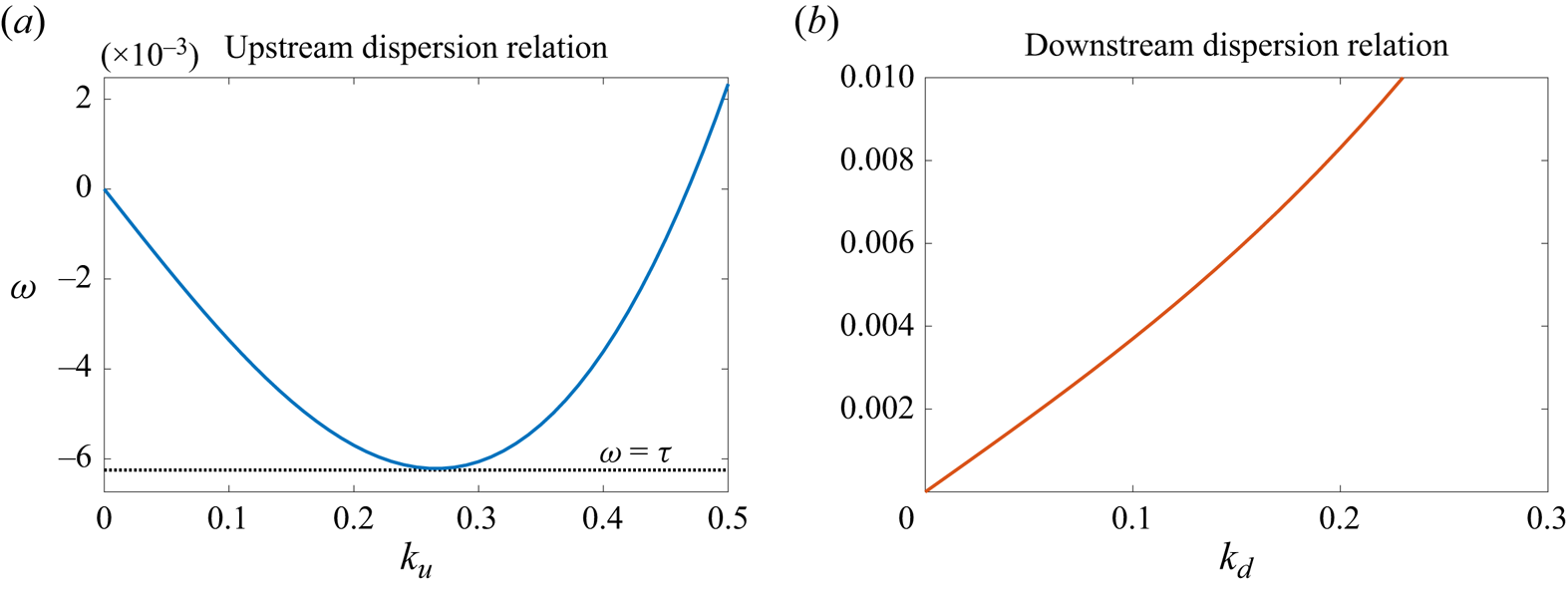
Figure 4. The dispersion curves for  $Fr=0.9659$ and $\gamma _s = 0.9550$ (corresponding to the hydraulic-fall solution when $a=-0.01$, $b=0.3$). (a) The upstream wave frequency $\omega$ as a function of the upstream wavenumber $k_{u}$. (b) The downstream wave frequency $\omega$ as a function of the upstream wavenumber $k_{d}$. The minimum $\omega = \tau = -0.006217$ of the upstream dispersion curve is shown with a dotted line in (a).
To calculate  $s_{ess}$ numerically, we set $\phi = -L$ at the upstream boundary $\varGamma _3$, and allow the upstream height to come as part of the solution (in so doing we are able to capture waves upstream), and we ‘pin’ the downstream height at the outflow boundary $\varGamma _1$. Since we do not constrain $\phi$ at the outflow boundary, this allows us to capture waves downstream. We filter out spurious essential modes by removing modes that grow as $x\to \pm \infty$; we found that a convenient empirical method of achieving this was to reject any eigenmode with $|\text {Re}(s_{ess})| > 10^{-7}$. We note that we do not apply the sponge layer in this calculation, i.e. we set $A_{\pm } = 0$.
The essential spectrum comprises two types of modes, denoted types I and  ${\rm II}$. Type ${\rm I}$ modes occur when $|\mathrm {Im}(s_{ess})| > |\tau |$. A set of calculations associated with a typical member of this class is shown in figure 5. In figure 5(a), $s_{ess}$ is shown on the imaginary axis in the complex $s$-plane for the underlying steady-state shown in figure 5(b) for $a=0.01$, $Fr=0.8823$. In figure 5(a) we highlight a particular member of $s_{ess}$, denoted $\lambda$, that satisfies $|\mathrm {Im}(\lambda )| > |\tau |$ (values quoted in the caption). The corresponding mode (real part) is shown in figure 5(c) and comprises two distinct wave patterns upstream and downstream, denoted $g_{u}$ and $g_{d}$, and highlighted in figures 5(d,e), respectively. The dominant wavenumbers of the type ${\rm I}$ modes can be determined, numerically, by calculating the power spectra of $g_{u}$ and $g_{d}$ as functions of the wavenumber $k$, as shown in figure 5(g). We calculate the power spectra using the fast Fourier transform (fft) of $g_{u}$ and $g_{d}$. For type ${\rm I}$ modes, there is a single dominant wavenumber for each of the upstream and downstream signals, as shown by the peak in each of the power spectra in figure 5(g). The wave numbers associated with these peaks correspond precisely to the intersections of the upstream and downstream dispersion curves with the horizontal line $\omega = +|\mathrm {Im}(\lambda )|$, as shown in figure 5(f), which has the same horizontal axis and scale as figure 5(g) to aid this comparison. This illustrates the excellent agreement between the theory and numerics, and gives us confidence in the fidelity of the numerical eigensolver.

Figure 5. Type  ${\rm I}$ modes of the numerically calculated $s_{ess}$ for the hydraulic-fall solution with $Fr=0.8823$, $a=0.01$, $b=0.3$. (a) The numerically computed $s_{ess}$ is shown with blue markers on the imaginary $s$ axis, and a particular element $s_{ess}=\lambda =0.1309\mathrm {i}$ is highlighted with a solid red marker. The horizontal dotted lines indicate the levels $s=\pm \mathrm {i}|\tau | = \pm 0.04489\mathrm {i}$; in this calculation, $|\mathrm {Im}(\lambda )| > |\tau |$. (b) The underlying steady state. (c) The real part of the eigenmode associated with $\lambda$. (d,e) The upstream/downstream portions of the real part of the eigenmode, denoted $g_{u}$ and $g_{d}$, respectively. (f) The downstream and upstream dispersion relations given in (3.8) and (3.9), respectively, with the minus sign taken in both cases. The dashed horizontal lines indicate $\omega = \pm |\mathrm {Im}(\lambda )|$. (g) The power spectrum, i.e. $|\texttt {fft}(\textit {g})|^2$ (the square of the Fourier transform). The horizontal axes of (f,g) are identical, so a direct comparison between the peaks of the power spectrum and the intersection of the dispersion curves with $\omega = \mathrm {Im}(\lambda )$ can be made. We also note that in (d–g), all calculations corresponding to the upstream section are shown as solid blue lines, while the downstream section use dotted yellow lines.
Type  ${\rm II}$ modes occur when $|\mathrm {Im}(s_{ess})| < |\tau |$. A set of calculations associated with a typical member of this class, denoted by $s_{ess} =\mu$, is shown in figure 6. This figure follows a structure identical to that of figure 5. In this class of modes, the upstream section of the mode, shown in figure 6(d), is clearly multi-harmonic. This is a direct consequence of the fact that in the upstream dispersion curve, for a given $|\omega | < |\tau |$, multiple values of $k_{u}$ satisfy (3.9). For type ${\rm II}$ modes, there are three dominant wavenumbers upstream, and one dominant wavenumber downstream. As for the type ${\rm I}$ modes, the wavenumbers associated with the peaks in the power spectra correspond precisely to the intersections of the upstream and downstream dispersion curves, but this time with the horizontal lines $\omega = \pm | \mathrm {Im}(\mu )|$, as shown in figures 6(f,g). For type ${\rm II}$ modes, the wavenumbers associated with $\omega = -|\mathrm {Im}(\mu )|$ will travel (as $t$ progresses) more slowly than the uniform upstream speed, while wavenumbers associated with $\omega = +|\mathrm {Im}(\mu )|$ will travel faster.

Figure 6. Type  ${\rm II}$ modes of the numerically calculated $s_{ess}$ for the hydraulic-fall solution with $Fr=0.8823$, $a=0.01$, $b=0.3$. The figure follows the same description as for figure 5, with the exception that in this calculation, we highlight a different member $s_{ess}=\mu =0.03027\mathrm {i}$ such that $|\mathrm {Im}(\mu )| < |\tau |$. Here, $\tau$ has the same value as in figure 5.
3.2.2. The point spectrum $s_{p}$

Throughout the following discussion, we will use  $\nu$ to represent the eigenvalue in the point spectrum $s_{p}$ that lies in the first quadrant of the complex plane. As was mentioned earlier, the point spectrum has a fourfold symmetry in the complex plane. In contrast to the forced solitary-wave fKdV calculations of Camassa & Wu (Reference Camassa and Wu1991) and Keeler et al. (Reference Keeler, Binder and Blyth2017), where the point spectrum eigenmodes are even-symmetric so that $g_{\hat {\eta },\nu }(-x) = g_{\hat {\eta },-\nu }(x)$, hydraulic-fall solutions are not even-symmetric, so we expect that $g_{\hat {\eta },\nu }(-x)\neq g_{\hat {\eta },-\nu }(x)$.
The numerical computation of the eigenmodes requires a great deal of care to filter out grid-dependent spurious modes. A very wide computational domain is needed because evanescent waves on the upstream or downstream side of the eigenmodes decay extremely slowly (this is quantified below). We identify two different types of mode in the point spectrum, which we term type  ${\rm III}$ corresponding to eigenvalues in the left half-plane (here $s_{p} = -\nu, -\nu ^*$), and type ${\rm IV}$ corresponding to eigenvalues in the right half-plane (here $s_{p} = \nu, \nu ^*$). To compute type ${\rm III}$ modes, we impose $y_f = \gamma _s$ and $\phi (L,y) = L$ at the outflow boundary $\varGamma _1$ so that the profile is flat downstream, but there are evanescent waves upstream. For type ${\rm IV}$ modes, we set $y_f=1$ and $\phi (-L,y) = -L$ at the inflow boundary $\varGamma _3$ to capture eigenmodes that are flat upstream and have evanescent waves downstream. We found empirically that a convenient way to filter out the spurious type ${\rm III}$/ ${\rm IV}$ modes was to reject any mode with eigenvalue in the right/left half-plane, respectively. We confirmed that the point spectra converge as the domain size $L$ is increased and the mesh resolution is made finer.
In figure 7, we show results for the negative forcing case  $a=-0.01$, $Fr=0.9659$. In figure 7(a), the point spectrum $s_{p}$ (green stars) is shown together with the essential spectrum $s_{ess}$ (blue circles) in the complex $s$-plane. The underlying steady state is shown in figure 7(b). Figures 7(c,d) show the corresponding ${\rm III}$ modes, and figures 7(e,f) show the corresponding ${\rm IV}$ modes. Note that the sponge layer is not included for either the type ${\rm III}$ or type ${\rm IV}$ calculations. The exponential decay rate of the type ${\rm IV}$ downstream waves is scrutinised in figure 7(g) by plotting the logarithm of the local wave maxima against $x$ and then estimating its slope. The decay rate is computed to be $-3.3\times 10^{-4}$.
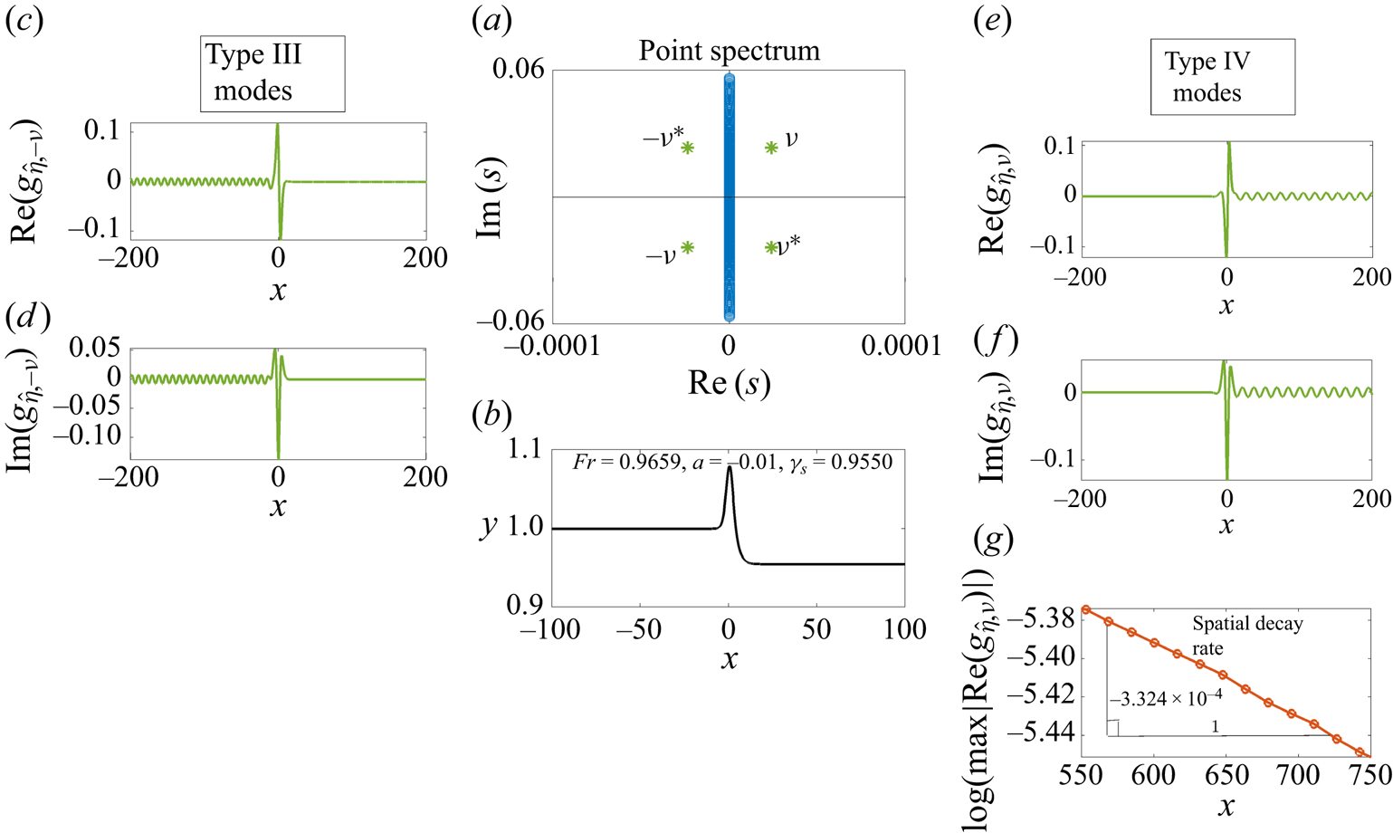
Figure 7. Type  ${\rm III}$ and ${\rm IV}$ modes of the numerically calculated $s_{p}$ for the hydraulic-fall solution with $Fr=0.9659$, $a=-0.01$, $b=0.3$. (a) Here, $s_{ess}$ is marked on the imaginary axis, and $s_{p}$ with $\nu = 2.375\times 10^{-5} + 0.0235\mathrm {i}$ is indicated with green stars. (b) The underlying steady state. (c,d) Type ${\rm III}$ eigenmodes corresponding to $s_{p}=-\nu,-\nu ^*$ (real and imaginary parts). (e,f) Type ${\rm IV}$ eigenmodes corresponding to $s_{p}=\nu,\nu ^*$. (g) Plot of $\log (\max |\mathrm {Re}(g_{\hat {\eta },\nu })|)$ against $x$, indicating the small spatial decay rate (estimated here) of the downstream wave in (e).
We find a non-empty point spectrum only when  $a<0$ (we calculated the essential and point spectrum for values of $a,b$ in the range $a^*< a<0.1$ and $0.3\leq b\leq 3.0$), and moreover, the point spectrum contains only four eigenvalues. We can investigate the linear instability for $a<0$ further by computing the point spectrum as $a$ is varied continuously. Figure 8 shows that as $a\to 0^-$, the quartet of eigenvalues appears to approach the origin. This is consistent with the fact that when $a=0$, i.e. for a flat bottom, the spectrum contains an isolated zero of multiplicity four (see, for example, Akers & Nicholls Reference Akers and Nicholls2012). As $a\to a^*\approx -0.016$, the unstable eigenmodes approach those found at the ‘termination point’ solutions discussed in § 3.1. The fact that we have not found a point spectrum when $a>0$ appears to suggest that hydraulic-fall solutions over positive bumps are linearly stable.
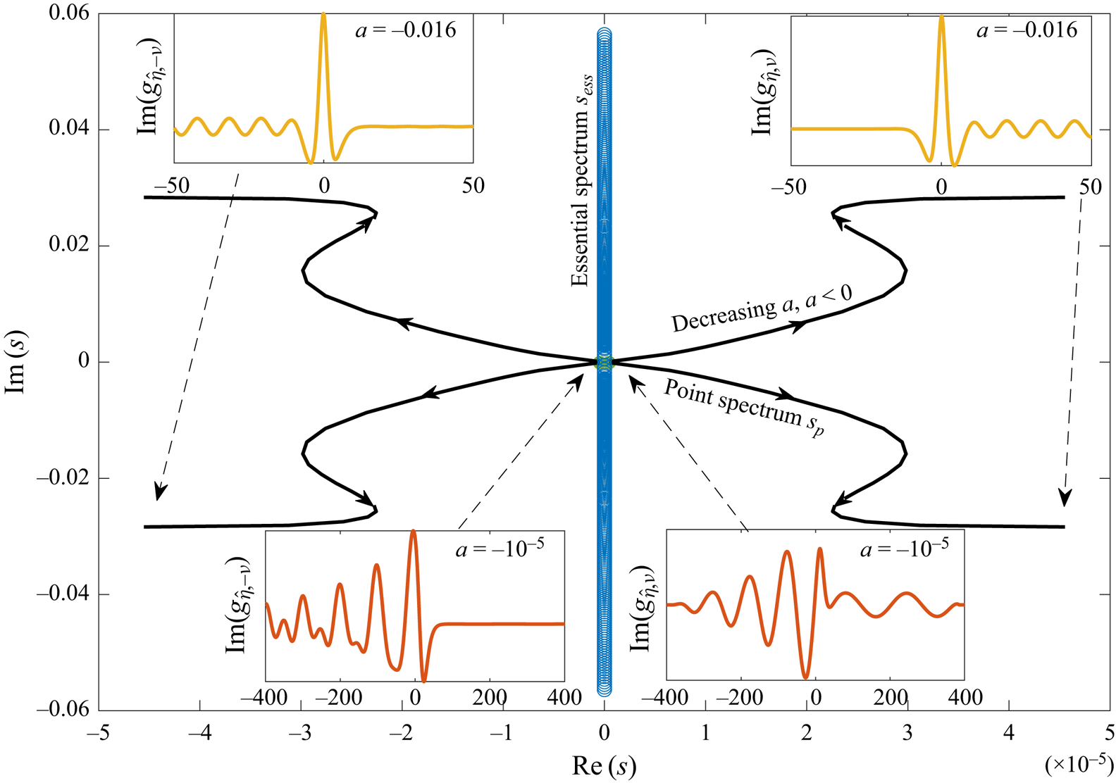
Figure 8. Hydraulic-fall solutions for  $b=0.3$, with numerically calculated $s_{p}$ as $a$ is varied (the corresponding values of $Fr$ can be inferred from figure 3). The solid black lines indicate $s_{p}$, and the arrows indicate how $s_{p}$ evolves as $a$ decreases from zero. Here, $s_{ess}$ is shown by hollow circular markers. We note that the eigenmodes of $s_{ess}$ change as $a$ is varied, but $s_{ess}$ itself remains on the imaginary axis. The insets show eigenmodes corresponding to $s_{p}$, as indicated by arrows for the values $a = -10^{-5}$ (bottom insets) and $a=-0.016\approx a^*$ (top insets).
Although we have analysed the stability properties of the linearised system, as is well known, linear stability does not imply nonlinear stability (see, for example, Holm et al. Reference Holm, Marsden, Ratiu and Weinstein1985). In the next subsection, we will perform numerical simulations to provide evidence for nonlinear stability.
3.3. Nonlinear stability
In this subsection, we solve an initial value problem in order to confirm the results of the previous section and to probe the nonlinear stability properties of the hydraulic-fall solutions. We introduce a localised perturbation to the steady solution  $y_s(x)$, taking
 \begin{equation} y_f(x,t=0) = y_s(x) + \varepsilon x\,\text{e}^{{-}a_2^2(x-a_3)^2}, \end{equation}
for some choice of the perturbation amplitude  $\varepsilon$ and the constants $a_2$ and $a_3$. In the results to be presented below, we choose $a_2=0.5$ in (3.11) and set $a_3 = 0$, but the general conclusion on the solution's stability remains the same for other values of $a_3$. The computation is carried out as follows. Having deformed the flow domain to incorporate the perturbation (3.11), we solve Laplace's equation over this domain together with the steady kinematic condition on the free surface $\varGamma _2$, (2.3), the no-penetration condition on the bottom $\varGamma _0$, (2.2), and the inflow and outflow conditions on $\varGamma _3$ and $\varGamma _1$, (2.7) and (2.8), respectively. This provides us with the initial velocity potential over the perturbed domain, namely $\phi (\boldsymbol {x},t=0)$. We set the downstream target level for the sponge layer as $y_+ = \gamma _s$.
Our stability analysis of the hydraulic-fall solutions depends on two parameters: the amplitude of the topographic forcing,  $a$, and the size of the perturbation, $\varepsilon$, in (3.11). To standardise the size of the perturbation as $a$ is varied, we set
 \begin{equation} \varepsilon = l\varDelta_s,\quad \varDelta_s \equiv |1-\gamma_s|, \end{equation}
with  $l>0$. This provides a convenient way to compare results for different values of $a$.
$a$.
As the system is Hamiltonian, the underlying dynamical system cannot contain attractors or repellers as the Hamiltonian is invariant along any trajectory in the system's phase space. Therefore, in this system, the stability properties of the steady states are interpreted by a local argument; the system can evolve towards/away from a steady state as energy is emitted far upstream/downstream.
When discussing the results of our numerical simulations, it will be useful to refer to the value of the ‘wave resistance coefficient’ that was introduced by Camassa & Wu (Reference Camassa and Wu1991) for the fKdV equation, which is defined as
 \begin{equation} C_r ={-}\int_{\varGamma_2}\frac{\partial y_{f}(x,t)}{\partial x}\,y_b(x)\,\text{d}S.\end{equation}
In the fKdV model,  $C_r$ is the power supplied by the bottom forcing $y_b$ (Camassa & Wu Reference Camassa and Wu1991).
3.3.1. Positive forcing
We start by examining hydraulic falls over a positive forcing with  $a>0$. Figure 9 shows the results of a time-dependent calculation using the initial condition (3.11) with $l=2.0$ (other parameter values are quoted in the caption). An animation of the time evolution of the free surface can be found in supplementary movie 1 (available at https://doi.org/10.1017/jfm.2024.599). Evidently, the system returns quickly to the original unperturbed stable state. It was found that this behaviour was typical for forcing amplitudes in the range $a=(0, 0.1]$ and perturbations in the range $l \in (0,4]$, providing evidence that the solution is stable to localised perturbations as prescribed in (3.11) for all $a>0$ sampled.

Figure 9. Perturbation of a hydraulic fall over positive forcing with  $a = 0.01$, $Fr = 0.88228$ and initial condition (3.11), with $l = 2.0$, $b=0.3$, $a_2 = 0.5$ and $a_3=0$. (a) Waterfall plot of free-surface evolution. (b) The initial perturbation (solid red line) and the steady state (dotted black line). (c) The free surface (solid red line) at $t=1247$ and the steady state (dotted black line).
3.3.2. Negative forcing
Figure 10 shows the result of a time-dependent calculation for a topographical dip with  $a=-0.01$, $b=0.3$ and initial condition (3.11) (the other parameter values are shown in the captions). We strongly recommend the reader to watch supplementary movie 2 to support the following discussion. A waterfall plot of the time evolution of the free surface is shown in figure 10(g). Figure 10(c) shows the time trace of $y_f(0,t)$ over the range $0< t<10^5$ (zoomed-in regions of this time trace are shown in figures 10(a,e)), and figure 10(d) shows the $(C_r,y_f(0,t))$ phase plane projection. The thicker lines in figure 10(d) indicate regions in phase space that are visited more frequently. Wave profiles at times $t=5000$ and $t=10^{5}$ are shown in figures 10(f,b), respectively.

Figure 10. Perturbation of the hydraulic-fall solution with  $a = -0.01$, $Fr = 0.9659$ (and $\varDelta _s = 0.0450$) with the initial condition (3.11) taking $l = 2.0$, $b=0.3$, $a_2=0.5$ and $a_3=0$. The underlying type ${\rm IV}$ eigenmode of the steady state has $\nu = 2.375\times 10^{-5} + 0.0235\mathrm {i}$. (a) Time trace of $y_f(0,t)$ over the window $8.6\times 10^4< t<9.15\times 10^5$. (b) Free-surface profile at $t=10^5$. The estimation of the wavenumber $k$ is indicated. (c) Time trace of $y_f(0,t)$ over $0< t<10^5$. The dotted line indicates $y_{s,f}(0)$. We note that the frequency of the oscillations cannot be resolved on this time scale, and zoomed regions are shown in (a,e). (d) The phase plane projection $(C_r,y_f(0,t))$ with the vertical axis on the same scale as (c). Thicker lines indicate locations in phase space that are visited more frequently. (e) Time trace of $y_f(0,t)$ over $0< t<5000$. (f) Free-surface profile at $t=5000$. The arrows indicate the direction of wave propagation. (g) Waterfall plot of free-surface evolution.
Considering these results, the time evolution can be divided broadly into two distinct stages. The initial stage (over  $0< t<5000$, say, and shown in figure 10(e)) is characterised by a roughly sinusoidal temporal oscillation of $y_f(0,t)$ about the steady-state value, the latter shown as a dotted line in figure 10(c). In this stage, the transient growth is well matched by the real part of the unstable eigenvalue $s=\nu$ of the underlying state, as shown by the dashed line in figure 10(c). The frequency of the oscillation is in excellent agreement with the imaginary part of $\nu$. In fact, the same observation holds for a broad range of topography amplitudes $a$. This is illustrated in figure 11(a), where $\text {Im}(\nu )$ is plotted against $a$. Also shown is the frequency of $y_f(0,t)$ estimated from the time trace during the initial stage of the evolution. Evidently, there is excellent agreement between the two. We also found that this frequency is independent of the perturbation amplitude $l$.
$l$.

Figure 11. (a) The frequency of oscillations in the initial stage of the evolution for the case studied in figure 10 but over a range of  $a$ values, and $b=0.3$. The solid lines are the imaginary part of $\nu$, and the line with circular markers is the estimate of the frequency from the time-dependent simulations. (b) The linear dispersion relation $\omega =\omega (k)$, with $k=k_d$, according to (3.8), shown with a dot-dashed curve. The estimated frequency–wavenumber relation for the small-amplitude waves emitted in figure 10(f) is illustrated with red circular markers. The (positive) imaginary part of the eigenvalue in the point spectrum, $\text {Im}(\nu )$, is shown with a solid blue line.
During this initial stage of the evolution, the amplitude of the oscillations increases and small-amplitude waves are emitted and travel downstream, as can be seen in of figure 10(f). We would expect that the wavenumber of these emitted waves conforms with the linear dispersion relation (3.8). We can test this by estimating the frequency and wavenumber of the emitted waves from the time signals and from the instantaneous free-surface profile, respectively. To approximate the frequency, we calculated the mean separation of the local maxima of the time signal  $y_f(0,t)$, and to estimate the wavenumber, we extracted the mean separation of the local maxima in the spatial wave profile $y_f(x,t)$ at $t=10^4$. The results are shown in figure 11(b), where we see good agreement with the dispersion relation $\omega =\omega (k)$, with $k=k_d$, in (3.8), although the disparity between the two increases as the wavenumber $k$ increases. Also shown in figure 11(b) is the (positive) imaginary part of the eigenvalue in the corresponding point spectrum (see § 3.2.2).
Eventually, the amplitude of the oscillations saturates, heralding the second evolutionary stage, which we refer to as the limiting stage. Here, the oscillations are less sinusoidal in character. The limiting stage is characterised by a regular stream of larger-amplitude cnoidal waves propagating in the upstream direction and away from the topographical dip, and, in contrast to the initial stage, the waves travelling downstream, as shown in figure 10(b), now consist of multi-harmonic waves. The phase-plane projection  $(C_r,y_f(0,t))$ shown in figure 10(d) has a distinctive guitar-pick shape. At large time $t$, the trajectory appears to have converged to a closed loop (shown in white with arrows), which represents an invariant solution of the system. We remark that this limiting behaviour was found to be typical for parameter values $a^*< a<0$, $0.3\leq b \leq 3.0$ and $l\in (0,4]$. We also recommend the reader to watch the animation in supplementary movie 3 focusing on how the limiting stage for figure 10 evolves over a temporal period.
In conclusion, the steady state hydraulic-fall solution with negative forcing is unstable, and perturbations from it settle down to a time-dependent, nonlinear stable invariant solution irrespective of size of the perturbation in (3.11). We discuss this in more detail in § 3.4.
3.3.3. Hydraulic rises
For completeness, we describe briefly the nonlinear stability of the steady hydraulic-rise solutions. Hydraulic rises are unstable for both positive and negative  $a$, as demonstrated in figures 12 and 13, respectively. For positive forcings, as the initial disturbance propagates downstream, a solitary wave emanates from the origin and moves upstream, whilst a steady cnoidal wave pattern emerges downstream. Ignoring the solitary wave, this structure is known as a generalised steady hydraulic rise (see figure 12). For negative forcings, similar to what was found for the hydraulic fall, the system settles into a time-periodic orbit as indicated in figure 13(c). We observe that the temporal signal of $y_f(0)$ in the limiting stage, as shown in figure 13(b), is more sinusoidal than that for the hydraulic fall (see figure 10a), and that a cnoidal wave pattern similar to that seen for the positively forced hydraulic rise emerges downstream.

Figure 12. Waterfall plot of free-surface evolution of a perturbation of a hydraulic rise over positive forcing with  $a = 0.01$, $Fr = 1.1173$ and initial condition (3.11), with $l = 2.0$, $b=0.3$, $a_2 = 0.5$ and $a_3=0$.

Figure 13. Hydraulic rise for the case  $a=-0.01$, $b=0.3$, $Fr = 1.0436$ and initial condition (3.11), with $l = 2.0$, $a_2 = 0.5$ and $a_3=0$. (a) Waterfall plot for the system starting from a state of near uniform flow. (b) Time trace of $y_f(0,t)$ in the limiting stage. (c) The projected phase plane $(C_r,y_f(0,t))$. The initial condition is shown as a circular marker, and the trajectory is in orange.
3.4. Time-dependent invariant solution
To explore further the existence of a time-dependent invariant solution for negative forcing,  $a<0$, we calculate the free-surface response when the system starts from a condition of near uniform flow with a flat free surface. Specifically, to provide the initial condition, we solve Laplace's equation over the flow domain shown in figure 2, but with a flat free surface $\varGamma _2$, enforcing the steady form of the free-surface kinematic condition, (2.3), the no-penetration condition on the bottom $\varGamma _0$, (2.2), and the inflow and outflow conditions on $\varGamma _3$ and $\varGamma _1$, (2.7) and (2.8), respectively. This yields the initial velocity potential $\phi (\boldsymbol {x},t=0)$. This starting condition is artificial as the pressure at the free surface does not match the constant ambient pressure at $t=0$, but we overlook this slight inconsistency. During the calculation we set the downstream sponge target level as $y_+ = 1$.
The results are shown in figure 14 for  $a=-0.01$ and $Fr=0.9659$, which are the same values as in figure 10. The waterfall plot shown in figure 14(a) indicates that the region left in the wake of the downstream travelling waves is itself wavy. The signal $y_f(0,t)$ shown in figures 14(b,c) appears to be periodic and is similar in character to the oscillations observed in figure 10(a). Furthermore, in figure 14(d), the trajectory in the $(C_r,y_f(0,t))$ plane is shown, and it is clear that the system is evolving towards the guitar-pick-shaped limiting orbit observed in figure 10, which is also shown (coloured white and labelled as the ‘limiting orbit’). This calculation provides further evidence of what appears to be a time-periodic orbit and that it is the same solution as in figure 10.

Figure 14. Hydraulic fall for the case  $a=-0.01$, $b=0.3$, $Fr = 0.9659$. (a) Waterfall plot for the system starting from a state of near uniform flow. (b) Time trace of $y_f(0,t)$. (c) Time trace in the period $9.5\times 10^{4}< t<10^{5}$. (d) The projected phase plane $(C_r,y_f(0,t))$. The initial condition is shown as a circular marker, the system trajectory is in red, and the limiting orbit from figure 10 is shown in white.
In figure 15, we examine the time-dependent invariant solution further by analysing the calculation in figure 10 for  $a=-0.01$. We begin by noting that, as can be seen in figure 15(a), the mean level of the downstream spatial signal, denoted $\overline {y_{d}}$, decreases as time progresses. Consequently, a modified downstream dispersion relation obtains for the limiting stage, and this is found by replacing $\gamma _s$ and $V$ in (3.8) with $\overline {y_{\infty }}$ and $1/\overline {y_{\infty }}$, respectively.

Figure 15. Frequency and wavenumber analysis of the downstream portion of the wave,  $y_{d}$, and the time signal $y_f(0,t)$, for the calculation in figure 10. (a) The downstream mean level $\overline {y_{d}}$ as a function of time. (b) The average frequency as $t$ varies, estimated from the local maxima of the time signal of $y_f(0,t)$. (c) The time signal of $y_f(0,t)$. (d) The power spectrum of the downstream wave in the limiting stage of the evolution, with the two peaks occurring at $k_1 \approx 0.2275$, $k_2\approx 0.3850$. (e) The power spectra of $y_f(0,t)$; note that the vertical axes is the frequency $\omega$, and the horizontal axis is the power. (f) The limiting stage dispersion curve together with the levels $\omega = \omega _1\approx 0.018$, $\omega _{2}\approx 0.036$. Note that the horizontal axis and scale are identical in (d,f), and the vertical axis and scale are identical in (e,f), to aid comparison. (g,h) The wave profile at the given time slot and the downstream portion of the free surface.
Next, we observe that the average temporal frequency, denoted  $\bar {\omega }$, estimated using the local maxima of the time signal $y_f(0,t)$ in figure 15(c), varies in time from a value close to $\bar {\omega } \approx \mathrm {Im}(\nu )$ in the initial stage of evolution to a smaller value, denoted $\omega _1$, in the limiting stage (see figure 15b). This frequency modulation can be explored further by calculating the power spectrum of the temporal signal of $y_f(0,t)$ in the limiting stage, i.e. over $10^5< t<1.5\times 10^5$. The result is shown in figure 15(e). This shows that there are actually two main temporal frequencies in the limiting stage, as indicated by the peaks in the temporal power spectra shown in figure 15(e). We denote these two dominant frequencies by $\omega _1\approx 0.018$ and $\omega _2\approx 0.036$.
In addition, we find there are two dominant wave numbers of the spatial downstream wave signal,  $y_{d}$ (see figure 15h), as indicated by the spatial power spectrum of $y_{d}$ at $t=10^5$ shown in figure 15(d). We denote these two dominant wave numbers by $k_1\approx 0.2275$ and $k_2\approx 0.3850$.
Bringing this all altogether, in figure 15(f) we show the limiting dispersion curve together with two horizontal lines indicating the levels  $\omega = \omega _1,\omega _2$. The values of $k$ where the curve intersects these lines correspond precisely to the two dominant wavenumbers $k_1, k_2$ seen in figure 15(d). To aid comparison across panels in the figure, the horizontal axes in figures 15(d,f) are identical, as are the vertical axes of figures 15(e,f). These results indicate that the wavenumbers of the downstream disturbance are linked to the temporal frequencies via the downstream dispersion curve.
In figure 16, we show the power spectrum of the time signal of  $y_f(0,t)$ at the limiting stage for a slightly different case with $a=-0.005$, $b=0.3$. The energy peak at the dominant frequency $\omega _1$ is evident, with other peaks of diminishing strength located approximately at $\omega = n\omega _1$, where $n=2,3,4,\ldots$, presumably generated via nonlinear effects. This is strong numerical evidence that the invariant solution is a periodic orbit. The downstream wavenumbers associated with the subharmonic frequencies $n\omega _1$ must satisfy the linear dispersion relation (3.8), and in general will be incommensurate. This explains the rather irregular appearance of the downstream waves in figure 15(h).

Figure 16. The power spectrum of  $y_f(0,t)$ in the limiting stage of the evolution for the solution when $a=-0.005$, $b=0.3$, $l=2$. The primary harmonic $\omega _1\approx 0.01257$ and the next three subharmonic frequencies are identified.
In summary, in this subsection we have obtained the most important result of the present paper, namely the apparent existence of a temporally periodic orbit of the fully nonlinear system. Time-periodic behaviour in free-surface flow over topography has been observed before, notably for the fKdV equation, by (Camassa & Wu Reference Camassa and Wu1991), Wu (Reference Wu1987) and Grimshaw & Smyth (Reference Grimshaw and Smyth1986). Through unsteady simulations, these authors found a similar oscillatory behaviour of the free surface over the topography. In this case, the period of the oscillation was linked to the frequency at which solitary waves were emitted in the upstream direction. However, in none of these studies was the long-time behaviour explored. It is also worth noting that this solution does not fall easily into any previously recognised class of time-periodic Euler free-surface flows. It is not spatially localised, and it is not spatially periodic. It cannot therefore be classified as a breather solution (see, for example, Peregrine Reference Peregrine1983), or as a standing wave, or as a travelling standing wave (Wilkening Reference Wilkening2021).
4. Conclusion
We have examined the stability of a hydraulic-fall flow over a localised bottom topography. The topography is in the form of a Gaussian whose amplitude is either positive (a bump) or negative (a dip). In the initial part of our analysis, we studied the linear stability of these solutions by first demonstrating that the full equations can be cast in the form of a canonical Hamiltonian system with a Hamiltonian that is a modification of that derived by Zakharov (Reference Zakharov1968) and Craig & Sulem (Reference Craig and Sulem1993) for the classical water wave problem. As a consequence, the spectrum of the system linearised about a steady hydraulic-fall solution has a fourfold symmetry in the complex plane.
In the case of a bump, our numerical computations showed that either the point spectrum is empty or else all of its eigenvalues are located on the imaginary axis so that the underlying flow is spectrally stable. For a dip, we identified a single eigenvalue in the point spectrum (to within the fourfold symmetry) that lies off the imaginary axis with a positive real part, meaning that the flow is linearly unstable. For both the bump and the dip, the essential spectrum occupies the whole of the imaginary axis. For both the bump and the dip, we carefully analysed the associated eigenfunctions, and we demonstrated that their behaviour in the far field, away from the localised topography, could be reconciled with the dispersion relation for small-amplitude waves over a flat bottom.
In the second part of our work, we examined the nonlinear stability properties by solving an initial value problem for the full Euler equations, with the initial condition taken to represent a small perturbation about a steady hydraulic fall. For a bump, the simulations showed that the disturbance to the free surface disperses so that the steady solution is ultimately recaptured. This is in keeping with the prediction of the linear stability analysis. Consequently, we concentrated most of our attention on the dip. In this case, our numerical simulations showed that the steady hydraulic fall is also nonlinearly unstable, and that ultimately the flow approaches a periodic state in which the free surface exhibits a localised peak that pulsates up and down over the dip, while small-amplitude waves are emitted continuously in both the upstream and downstream directions. This periodic state may be interpreted as an invariant solution of the underlying dynamical system. We have shown numerically that the periodic waves that are emitted downstream have a dominant temporal frequency that can be linked accurately to the linear dispersion relation based on the mean downstream depth. The subharmonic frequencies of these waves were found to be rational multiples of the dominant frequency, thereby reinforcing our conclusion that a periodic state has been achieved.
Interesting questions remain. For example, beside periodic solutions as identified here, there exists the possibility of quasi-periodic solutions. Such objects exist in phase space as so-called invariant tori (e.g. Kuznetsov Reference Kuznetsov1998). However, directly calculating time-dependent invariant solutions, such as periodic orbits or invariant tori, remains a highly non-trivial numerical task. In other applications in fluid dynamics, periodic orbits have been computed semi-analytically using a weakly nonlinear approach, e.g. for air bubbles in a Hele-Shaw channel (Keeler et al. Reference Keeler, Thompson, Lemoult, Juel and Hazel2019). Page & Kerswell (Reference Page and Kerswell2018, Reference Page and Kerswell2019) have recently applied Koopman analysis and dynamic mode decomposition to approximate periodic orbits for the Burgers equation and the Navier–Stokes equations. Another possibility is to adapt the methodology for calculating travelling-wave solutions that are periodic in space and time from Wilkening (Reference Wilkening2011) and Wilkening & Zhao (Reference Wilkening and Zhao2021). It would be of interest to understand whether these methods can be implemented for the non-localised and non-spatially periodic solution discussed here in order to further probe the landscape of invariant solutions in phase space.
Finally, as was noted in the Introduction, there is an apparent lack of experimental results in the literature concerning hydraulic falls over a dip. It would be of interest to see if the numerical observations in the present work, and in particular the time-periodic flow that appears at large time, can be realised in the laboratory.
Supplementary movies
Supplementary movies are available at https://doi.org/10.1017/jfm.2024.599.
Funding
J.S.K. acknowledges funding from the Leverhulme Trust (ECF-2021-017).
Declaration of interests
The authors report no conflict of interest.
Author contributions
Both authors contributed to developing the theory and results in this paper. The numerical model and numerical calculations were developed and performed by J.S.K.


 Open access