


1. Introduction
The displacement of one fluid by another in porous media is commonly encountered in environmental and industrial flows. When the injected fluid is more viscous than the displaced one, the displacement is hydrodynamically stable and the interface between both fluids remains planar. In the reverse situation where the invading fluid is less viscous than the displaced one, the interface shows a finger-like deformation because the interface is hydrodynamically unstable with regard to a viscous fingering (VF) instability (Engelberts & Klinkenberg Reference Engelberts and Klinkenberg1951; Saffman & Taylor Reference Saffman and Taylor1958; Homsy Reference Homsy1987). VF with or without chemical reactions has been well studied so far (Homsy Reference Homsy1987; McCloud & Maher Reference McCloud and Maher1995; De Wit Reference De Wit2020) because of its wide range of applications such as in transport of digestive juices (Bhaskar et al. Reference Bhaskar, Grik, Turner, Bradley, Bansil, Stanley and LaMont1992), chromatography (Broyles et al. Reference Broyles, Shalliker, Cherrak and Guiochon1998; Haudin et al. Reference Haudin, Callewaert, De Malsche and De Wit2016), secondary and ternary oil recovery (Lake et al. Reference Lake, Johns, Rossen and Pope2014; Sabet et al. Reference Sabet, Mohammadi, Zirahi, Zirrahi, Hassanzadeh and Abedi2020) and  ${\rm CO}_{2}$ sequestration (Berg & Ott Reference Berg and Ott2012) to name a few. In the miscible displacement of a solution of $B$ of viscosity $\mu _b$ by a solution of $A$ of viscosity $\mu _a$, an important parameter controlling VF is the log-mobility ratio $R_b=\ln (\mu _b/\mu _a)$. If $R_b >0$, the displacement is unstable and VF is all the more vigorous if $R_b$ is increased or the flow rate is larger (Homsy Reference Homsy1987). The $R_b <0$ case is stable, leading to stable planar interfaces in non-reactive systems.
Fingering patterns can be modified by reactions which change viscosity, permeability or interfacial tension (Nagatsu Reference Nagatsu2015; De Wit Reference De Wit2016, Reference De Wit2020). Experiments have provided evidence for, for example, changes in the fingering pattern due to a decrease in interfacial tension induced by a reaction in immiscible systems (Fernandez & Homsy Reference Fernandez and Homsy2003; Tsuzuki et al. Reference Tsuzuki, Ban, Fujimura and Nagatsu2019) or due to a decrease in permeability by a precipitation reaction in miscible systems (Nagatsu et al. Reference Nagatsu, Bae, Kato and Tada2008, Reference Nagatsu, Ishii, Tada and De Wit2014; Haudin & De Wit Reference Haudin and De Wit2015; Shukla & De Wit Reference Shukla and De Wit2016). When a chemical reaction affects the VF dynamics, the value of the dimensionless Damköhler number  $D_a$ defined as the ratio of the characteristic time of advection to that of the chemical reaction is an additional important parameter.
From a theoretical point of view, miscible reactive VF for which the reaction induces in situ a change in viscosity has been investigated numerically in the case of a bistable chemical reaction changing the viscosity across a moving chemical front, inducing a new mechanism of ‘droplet’ formation (De Wit & Homsy Reference De Wit and Homsy1999). Later, linear stability analysis (Hejazi et al. Reference Hejazi, Trevelyan, Azaiez and De Wit2010; Kim et al. Reference Kim, Pramanik, Sharma and Mishra2021) and nonlinear simulations (Gérard & De Wit Reference Gérard and De Wit2009; Nagatsu & De Wit Reference Nagatsu and De Wit2011; Sharma et al. Reference Sharma, Pramanik, Chen and Mishra2019; Kim et al. Reference Kim, Pramanik, Sharma and Mishra2021; Tafur et al. Reference Tafur, Escala, Soto and Munuzuri2021; Verma, Sharma & Mishra Reference Verma, Sharma and Mishra2022) have classified the stabilising or destabilising influence of simple  $A + B \rightarrow C$ reactions on VF. For such simple bimolecular reactions, an important parameter is the log-mobility ratio $R_c = \ln (\mu _c/\mu _a)$ comparing the viscosities of equimolar solutions of the product $C$ or reactant $A$. Most theoretical works on this reactive VF have considered the case where the initial concentration of $A$ and $B$ is the same and all species diffuse at the same rate. Under this condition, if $R_c=R_b$, the product has the same viscosity as the reactant $B$ and the reactive case is exactly the same as the non-reactive one. If $R_c< R_b$, the reaction decreases the viscosity while viscosity increases if $R_c>R_b$. As long as $0 < R_c < 2R_b$, the viscosity profile remains monotonic. An extremum in viscosity is observed if $R_c <0$ or $R_c > 2R_b$. When $R_b <0$ and there is an extremum in viscosity, modelling predicts that, similarly to differential diffusion effects (Mishra et al. Reference Mishra, Trevelyan, Almarcha and De Wit2010), reactions are able to destabilise otherwise stable displacements thanks to the build-up of non-monotonic viscosity profiles (Hejazi et al. Reference Hejazi, Trevelyan, Azaiez and De Wit2010; Nagatsu & De Wit Reference Nagatsu and De Wit2011; Riolfo et al. Reference Riolfo, Nagatsu, Iwata, Maes, Trevelyan and De Wit2012; Escala et al. Reference Escala, De Wit, Carballido-Landeira and Munuzuri2019).
In 2007, Nagatsu et al. (Reference Nagatsu, Matsuda, Kato and Tada2007) reported the first experimental study of miscible VF with viscosity changes induced by a very fast chemical reaction (infinite  $D_a$) during a radial injection in a Hele-Shaw cell. In this study, polymer solutions with viscosity depending on pH were displaced by less-viscous acid or base aqueous solutions ( $R_b >0$ case). The reaction modifies locally the gradient in viscosity but the viscosity profile remains monotonically increasing. It was shown that, at fixed large flow rates, reactive VF patterns have a larger surface density, i.e. cover a larger area than their non-reactive equivalent at given times and flow rates when the reaction increases the viscosity. This is due to the fact that the reaction widens the fingers and decreases the shielding effect. In contrast, in the case of a decrease in viscosity by reaction, the surface density of the VF patterns is lower, i.e. fingers are thinner and shielding is enhanced. Subsequently, similar reactive VF experiments with monotonic increasing viscosity profiles have been performed under moderate $D_a$ conditions using slower reactions for both chemically driven viscosity decrease (Nagatsu et al. Reference Nagatsu, Kondo, Kato and Tada2009) and increase (Nagatsu et al. Reference Nagatsu, Kondo, Kato and Tada2011). It was shown that, for such intermediate $D_a$ conditions, the experimental results were opposite to those of the infinite $D_a$ case, i.e. the area occupied by the VF pattern was increased (decreased) in case of viscosity decrease (increase).
In the case of reactive VF ( $R_b >0$) with non-monotonic viscosity profiles featuring a maximum, experiments have shown that the maximum induces fingers extending preferentially towards the back of the reaction zone (Bunton et al. Reference Bunton, Tullier, Meiburg and Pojman2017). By increasing experimentally the Damköhler number, the stabilising effect of the reaction can as well be enhanced (Stewart et al. Reference Stewart, Marin, Tullier, Pojman, Meiburg and Bunton2018). The reactive destabilisation of an otherwise stable front ( $R_b<0$) has been achieved experimentally in the case of the reactive displacement of acid or base aqueous solutions by a more-viscous polymer solution showing that the chemically induced pattern is different depending on whether the reaction builds a maximum or a minimum (Riolfo et al. Reference Riolfo, Nagatsu, Iwata, Maes, Trevelyan and De Wit2012). Destabilisation induced by a pH sensitive clock reaction has also shown how the reactive feedback of a pH-changing reaction on viscosity can control fingering (Escala et al. Reference Escala, De Wit, Carballido-Landeira and Munuzuri2019; Escala & Munuzuri Reference Escala and Munuzuri2021). The destabilisation of the case of reactant solutions of same viscosities, i.e. $R_b=0$ has been studied experimentally by Podgorski et al. (Reference Podgorski, Sostarecz, Zorman and Belmonte2007).
Numerical simulations of reactive miscible VF with viscosity changes by an instantaneous  $A + B \rightarrow C$ chemical reaction for infinite $D_a$ conditions (Nagatsu & De Wit Reference Nagatsu and De Wit2011) and variable $R_b$ and $R_c$ are in good agreement with the experimental results (Nagatsu et al. Reference Nagatsu, Matsuda, Kato and Tada2007), i.e. an increase (decrease) of viscosity by the reaction leads to surface denser (less-dense) VF patterns. For $R_b=0$, the effect on the properties of reactive fingering of varying the Damköhler number, the contrast in viscosity between products and reactant, the initial concentrations, and the diffusion coefficients (Gérard & De Wit Reference Gérard and De Wit2009; Verma et al. Reference Verma, Sharma and Mishra2022) are in good agreement with the experiments from Podgorski et al. (Reference Podgorski, Sostarecz, Zorman and Belmonte2007). In particular, Gérard & De Wit (Reference Gérard and De Wit2009) showed that, even if the solutions of the two reactants $A$ and $B$ have the same viscosity, the VF pattern is different whether $A$ is injected into $B$ or the reverse as soon as these reactants have different diffusion coefficients or different initial concentrations because the underlying concentration profiles controlling the viscosity profile are not symmetric. This study was however limited to the case $R_b=0$ and did not investigate the effect of changing the value of $Pe$.
$Pe$.
The effect of varying the Péclet number has been investigated numerically as well, showing that, as expected, decreasing  $Pe$ for non-reactive cases stabilises VF (Homsy Reference Homsy1987; Pramanik & Mishra Reference Pramanik and Mishra2015; Shukla & De Wit Reference Shukla and De Wit2020). Interestingly, Hejazi & Azaiez (Reference Hejazi and Azaiez2010) show that, for $A + B \rightarrow C$ reactions with moderate $D_a$, larger $Pe$ can lead to slower rates of chemical production, i.e. less product $C$ generated at a same time. This is attributed to the fact that the mixing between reactants by diffusion is then less efficient at early times. Shukla & De Wit (Reference Shukla and De Wit2020) have performed a numerical study of the effect of $A + B \rightarrow C$ reactions on VF when varying $Pe$ for a finite $D_a$ and equal diffusion coefficients, focusing on the case of a viscosity-decreasing reaction both in the case of monotonic and non-monotonic viscosity profiles. They found that the viscosity-decreasing reaction has an increased stabilising effect when $Pe$ is decreased in the sense that the mixing length of species $A$ at given times is smaller in the reactive case than that in the non-reactive one when $Pe$ is lower. This effect was attributed to a build-up of a minimum in the viscosity profile. However, the mixing lengths of species $B$ and $C$ at given times in the reactive case were larger than those in the non-reactive case and the study focused on equal diffusion coefficients only.
It is of interest to study to what extent overall stabilisation can also be obtained for monotonic profiles and what is the role of differential diffusion effects. Moreover, experiments on miscible VF with  $A + B \rightarrow C$ reactions for which the Péclet number is varied in a wide range are not yet available.
In this context, we have experimentally investigated the influence of changes in the injection flow rate or, equivalently, changes in the Péclet number  $Pe$ on miscible VF when a bimolecular $A + B \rightarrow C$ reaction decreases viscosity. In the experiments, we analyse the change in the VF patterns when viscous polymer solutions are displaced by a less-viscous acidic solution such that the viscosity is decreased in situ via reaction-driven pH changes. Scanning a wide range of flow rates, we show that this reaction-driven viscosity decrease has opposite effects on the VF pattern at high and low flow rates, respectively. Interestingly, for lower flow rates, a full stabilisation of the interface by reaction is obtained. In parallel, a numerical investigation of the influence of changes in the Péclet number $Pe$ on VF for a viscosity decreasing reaction with monotonic viscosity profiles confirms the same trend provided the injected reactant diffuses sufficiently faster than the displaced one. Our findings pave the way to devise a control of VF by chemical reactions choosing suitable reactants and flow conditions.
2. Experimental set-up and numerical description
2.1. Experimental set-up
Experiments are conducted in a horizontal Hele-Shaw cell consisting in two glass plates separated by a thin gap in which a viscous fluid is displaced by another less-viscous one, injected through a central hole at a fixed flow rate (see figure 1). The gap of the cell  $b$ is fixed to 0.3 mm and the injection flow rate $q$ is varied from $9.2 \times 10^{-11}$ to $3.6 \times 10^{-8}\ {\rm m}^{3}\ {\rm s}^{-1}$. In reactive displacements, the displaced more-viscous solution is a 0.125 wt % sodium polyacrylic acid (SPA) solution (molecular weight of $2.1\unicode{x2013}6.6 \times 10^6$) while the injected displacing less-viscous fluid is a 0.2 M HCl aqueous solution. Upon contact between these solutions, a chemical reaction produces polyacrylic acid (PAA), resulting in a viscosity decrease at an instantaneous rate (Nagatsu et al. Reference Nagatsu, Matsuda, Kato and Tada2007, Reference Nagatsu, Iguchi, Matsuda, Kato and Tada2010).
Schematic of the Hele-Shaw cell reactor.

For the non-reactive case, the same 0.125 wt % SPA solution and deionised water are used as the more- and less-viscous solutions, respectively. In all cases, the less-viscous solutions are dyed with trypan blue for visualisation of the dynamics. The viscosity of the various fluids was measured using a commercial viscosimeter (from TA Instruments, Japan). The viscosity of the more-viscous polymer solution is shear thinning, i.e. decreases with the shear rate as shown by the blue squares in figure 2. The viscosities of the displacing dyed Newtonian 0.2 M HCl aqueous solution or pure water are 1.1 and 1.0 mPa $\cdot$s, respectively. We also measured the viscosity of a mixture of equal volumes of 0.125 wt % SPA solution and 0.2 M HCl solution (in the reactive case) and that of 0.125 wt % SPA solution and water (in the non-reactive case), see figure 2. We find that the viscosity in the reactive mixture system is much lower than that in the non-reactive one and that the reaction, in effect, decreases the viscosity.
Viscosity as a function of shear rate of the more-viscous fluid (blue squares) and that of the solution obtained by mixing equal volumes of a 0.125 wt % SPA solution and of a solution of 0 M (black circles) or 0.2 M HCl (red triangles) including 0.1 wt % trypan blue.

2.2. Numerical simulations
To simulate the experiments shown above, we consider a horizontal Hele-Shaw cell of length  $L_x$ and width $L_y$ with constant permeability $\kappa$ in which a miscible solution of reactant $A$ with viscosity $\mu _A$ is injected from left to right into a polymer solution of reactant $B$ with viscosity $\mu _B$ at a constant speed $U$ along the $x$ direction (figure 3). A bimolecular $A + B \rightarrow C$ reaction giving the product $C$ with viscosity $\mu _C$ takes place in the contact zone between reactants $A$ and $B$. Here, species $A$,
$A$,  $B$ and $C$ correspond to HCl, SPA and PAA, respectively in the experiment. As in experiments, we follow the dynamics by the spatiotemporal evolution of the neutral dye, $E$, initially dissolved in the injected solution. We assume that buoyant effects are negligible and that the fluids are incompressible. The dynamics is described by Darcy's law coupled to reaction–diffusion–advection equations for the concentrations:
 $$\begin{gather} \boldsymbol{\nabla}\boldsymbol{\cdot}\boldsymbol{u} = 0, \end{gather}$$
 $$\begin{gather}\boldsymbol{\nabla} p =-\frac{\mu(b,c)}{\kappa} \boldsymbol{u}, \end{gather}$$
 $$\begin{gather}\frac{\partial a}{\partial t} + \boldsymbol{u}\boldsymbol{\cdot}\boldsymbol{\nabla} a = D_A\nabla^2a - kab, \end{gather}$$
 $$\begin{gather}\frac{\partial b}{\partial t} + \boldsymbol{u}\boldsymbol{\cdot}\boldsymbol{\nabla} b = D_B\nabla^2b - kab, \end{gather}$$
 $$\begin{gather}\frac{\partial c}{\partial t} + \boldsymbol{u}\boldsymbol{\cdot}\boldsymbol{\nabla} c = D_C\nabla^2c + kab, \end{gather}$$
 $$\begin{gather}\frac{\partial e}{\partial t} + \boldsymbol{u}\boldsymbol{\cdot}\boldsymbol{\nabla} e = D_E\nabla^2e, \end{gather}$$
 $$\begin{gather}\mu(b,c) = \mu_A \exp\left( R_b \frac{b}{f_0} + R_c \frac{c}{f_0} \right), \end{gather}$$
where  $\mu _A$, $\mu _B$ and $\mu _C$ are the viscosities of the solutions of $A$,
$A$,  $B$ and $C$ at a same reference concentration $f_0$. Here $a$,
$a$,  $b$,
$b$,  $c$ and $e$ denote the concentrations of the reactants $A$ and $B$, the product $C$ and the dye $E$, respectively; $\boldsymbol {u}=(u,v)$ is the two-dimensional velocity; $k$ is the kinetic constant; $p$ is the pressure; $D_I$ is the diffusivity coefficient of species $I$;
$I$;  $\mu (b,c)$ is the viscosity; $R_b$ and $R_c$ are the log-mobility ratio defined as
 \begin{equation} R_b = \ln \left(\frac{\mu_B}{\mu_A} \right) , \quad R_c = \ln \left(\frac{\mu_C}{\mu_A} \right).\end{equation}
Note that, except for (2.7), the formulation is equivalent to the model of Shukla & De Wit (Reference Shukla and De Wit2020). For the non-reactive case, the system is hydrodynamically unstable when the less-viscous solution of  $A$ displaces the more-viscous solution of $B$, i.e. when $\mu _A<\mu _B$ or $R_b>0$. To mimic the fact that the reaction decreases viscosity in the experiments (see figure 2), we consider here $R_b=2$ and $R_c=0$ such that the product $C$ is less viscous than the reactant $B$ but we keep a monotonic viscosity profile.
Two-dimensional porous medium of length  $L_x$ and width $L_y$ with permeability $\kappa$ in which a miscible solution of reactant $A$ with viscosity $\mu _A$ is injected from left to right into a solution of reactant $B$ with viscosity $\mu _B>\mu _A$ at a constant speed $U$ along the $x$ direction. Here, $a_0$, $b_0$ and $e_0$ are the initial concentration of reactant $A$, reactant $B$ and dye $E$, respectively.

2.3. Non-dimensional equations
To specifically let the Péclet number appear in the dimensionless problem, the reference scales for length, velocity, time, concentration, viscosity, diffusivity and pressure are taken as  $L_y$, $U$,
$U$,  $L_y/U$, $f_0$, $\mu _A$, $D_C$ and $\mu _AUL_y/\kappa$, respectively. For simplicity, equations are written in a reference frame moving with speed $U$ with $\boldsymbol {e_x}$ being the unit vector along $x$ direction. The dimensionless forms of (2.1)–(2.8a,b) can be written as
 $$\begin{gather} \boldsymbol{\nabla}\boldsymbol{\cdot}\boldsymbol{u} = 0, \end{gather}$$
 $$\begin{gather}\boldsymbol{\nabla} p =-\mu(b,c)(\boldsymbol{u}+\boldsymbol{e_x}), \end{gather}$$
 $$\begin{gather}\frac{\partial a}{\partial t} + \boldsymbol{u}\boldsymbol{\cdot}\boldsymbol{\nabla} a =\frac{\delta_A}{Pe}\nabla^2a - D_aab, \end{gather}$$
 $$\begin{gather}\frac{\partial b}{\partial t} + \boldsymbol{u}\boldsymbol{\cdot}\boldsymbol{\nabla} b =\frac{\delta_B}{Pe}\nabla^2b - D_aab, \end{gather}$$
 $$\begin{gather}\frac{\partial c}{\partial t} + \boldsymbol{u}\boldsymbol{\cdot}\boldsymbol{\nabla} c =\frac{1}{Pe}\nabla^2c + D_aab, \end{gather}$$
 $$\begin{gather}\frac{\partial e}{\partial t} + \boldsymbol{u}\boldsymbol{\cdot}\boldsymbol{\nabla} e =\frac{\delta_E}{Pe}\nabla^2e, \end{gather}$$
 $$\begin{gather}\mu(b,c) = \exp(R_bb + R_cc), \end{gather}$$
where  $D_a=kf_0 L_y/U=\tau _h/\tau _c$ is the dimensionless Damköhler number defined as the ratio of the hydrodynamic time scale $\tau _h=L_y/U$ to the chemical time scale $\tau _c=1/kf_0$. The Péclet number $Pe=UL_y/D_C=\tau _D/\tau _h$ is the ratio of the diffusive time $\tau _D=L_y^2/D_C$ and the advective time $\tau _h$ while $\delta _A=D_A/D_C$, $\delta _B=D_B/D_C$ and $\delta _E=D_E/D_C$ are the diffusion coefficient ratios (Shukla & De Wit Reference Shukla and De Wit2020). Taking the curl of the momentum equation and defining the stream function $\psi$ as $u=\partial \psi /\partial y$ and $v=-\partial \psi /\psi x$, we obtain
 $$\begin{gather} \nabla^2\psi = R_b\left(\frac{\partial\psi}{\partial x}\frac{\partial b}{\partial x} + \frac{\partial\psi}{\partial y}\frac{\partial b}{\partial y} + \frac{\partial b}{\partial y} \right) + R_c\left(\frac{\partial\psi}{\partial x}\frac{\partial c}{\partial x} + \frac{\partial\psi}{\partial y}\frac{\partial c}{\partial y} + \frac{\partial c}{\partial y} \right), \end{gather}$$
 $$\begin{gather}\frac{\partial a}{\partial t} + \frac{\partial\psi}{\partial y}\frac{\partial a}{\partial x} - \frac{\partial\psi}{\partial x}\frac{\partial a}{\partial y} = \frac{\delta_A}{Pe}\nabla^2a - D_aab, \end{gather}$$
 $$\begin{gather}\frac{\partial b}{\partial t} + \frac{\partial\psi}{\partial y}\frac{\partial b}{\partial x} - \frac{\partial\psi}{\partial x}\frac{\partial b}{\partial y} = \frac{\delta_B}{Pe}\nabla^2b - D_aab, \end{gather}$$
 $$\begin{gather}\frac{\partial c}{\partial t} + \frac{\partial\psi}{\partial y}\frac{\partial c}{\partial x} - \frac{\partial\psi}{\partial x}\frac{\partial c}{\partial y} = \frac{1}{Pe}\nabla^2c + D_aab, \end{gather}$$
 $$\begin{gather}\frac{\partial e}{\partial t} + \frac{\partial\psi}{\partial y}\frac{\partial e}{\partial x} - \frac{\partial\psi}{\partial x}\frac{\partial e}{\partial y} = \frac{\delta_E}{Pe}\nabla^2e. \end{gather}$$
 The initial conditions for the stream function and product concentration are taken as  $\psi (x,y)=0$ and $c(x,y)=0$, for all ( $x,y$). For the initial concentrations of the reactant $A$ and $B$ solutions, we use a step function between $a=10$, $b=0$ on the left and $b=1$, $a=0$ on the right of $x=x_0$ where $x_0$ is the initial position of the interface with a random noise of amplitude of order $10^{-2}$ added in the front to trigger the instability. To solve (2.16)–(2.20), we use a pseudo-spectral method based on Fourier coefficients (Tan & Homsy Reference Tan and Homsy1988; Gérard & De Wit Reference Gérard and De Wit2009; Pramanik & Mishra Reference Pramanik and Mishra2015). The numerical domain has a size of $1024 \times 256$ for $Pe \leq 2000$ and $4096 \times 1024$ for $Pe =4000$ and 8000. Boundary conditions are periodic in both directions. This is standard for the transverse direction and yields good results along the longitudinal direction as long as the length $L_x$ is taken sufficiently long for the two fronts not to interact. Figures of the fingering dynamics focus on the unstable front.
Note that, for a given reference concentration  $f_0$ and geometry, the diffusive and chemical time scales $\tau _d$ and $\tau _c$ are constant. Our simulations aim to investigate the effects of varying the flow rate. To do so, we vary $U$ and hence $Pe$ by changing $\tau _h$. As $Pe=\tau _d/\tau _h$ and $D_a=\tau _h/\tau _c$, we have that $Pe{\cdot } Da={\rm const.}$ such that any change in $Pe$ implies a change in $D_a$ as well (Escala & Munuzuri Reference Escala and Munuzuri2021). Here, we fix $Pe{\cdot } Da=8000$.
3. Results and discussion
3.1. Displacement experiments
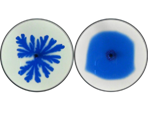
Experimental results comparing unstable displacements with or without reaction are shown in figure 4. First, we see that, as expected, increasing the flow rate allows to reach the same position much faster in both cases. In the non-reactive case, especially at lower flow rates, the pattern features very branched fingers, similar to those observed in other non-Newtonian systems (Nittman, Daccord & Stanley Reference Nittman, Daccord and Stanley1985; Zhao & Maher Reference Zhao and Maher1992; Kawaguchi Reference Kawaguchi2001). In contrast, in the higher-flow-rate regime, the dynamics is rather similar to those seen with Newtonian non-reactive fluids with less-branched patterns owing to the shear-thinning viscosity and the higher shear rate. Note that the sharpness of the viscosity profile along the gap direction may also play a role (Lajeunesse et al. Reference Lajeunesse, Martin, Rakotomalala and Salin1997; Videbaek & Nagel Reference Videbaek and Nagel2019; Keable et al. Reference Keable, Jones, Krevor, Muggeridge and Jackson2022) as seen when, for instance, the colour becomes less intense around the fingertip (Videbaek & Nagel Reference Videbaek and Nagel2019; Keable et al. Reference Keable, Jones, Krevor, Muggeridge and Jackson2022). In our experimental results, the colour intensity of the dye is almost uniform over the whole VF pattern as shown in figures 4 and 7. Hence, we do not explore the three-dimensional structure of the fingers any further. This is also motivated by the fact that ratios of viscosities  $\mu _B/\mu _A$ are here typically of the order of $10^2$– $10^3$ depending on flow rate and position along the radius so that we do not expect here to see patterns with proportionate growth as observed at lower viscosity ratios when flow rate is varied (Bischofberger, Ramachandran & Nagel Reference Bischofberger, Ramachandran and Nagel2014; Videbaek & Nagel Reference Videbaek and Nagel2019).
Displacement patterns comparing for different injection flow rates the non-reactive cases (upper line) and the reactive cases (bottom line) at the time (given in each panel) when the longest finger has reached the distance  $r_{max}=0.8r_{HS}$ where $r_{HS}=58$ mm is the radius of the cell.

As seen qualitatively in figure 4 and quantitatively in figure 5 (see Appendix B for details on finger width measurements), the typical finger width does not depend much on the injection flow rate  $q$ for the non-reactive case. To understand this, we recall that, because of the shear thinning fluid property of the more-viscous fluid, its apparent viscosity and, hence, the viscosity contrast between the two solutions is decreasing with an increase in the flow rate. This stabilising effect is counterbalanced by the fact that, classically, an increase in the flow rate increases the fingering destabilisation (Homsy Reference Homsy1987). Hence, the balance between both effects induces that the typical finger width of the non-reactive pattern is almost independent of the flow rate. Similar effects occur in VF of non-Newtonian immiscible fluids as well (Bonn et al. Reference Bonn, Kellay, Ben Amar and Meunier1995; Singh, Lalitha & Mondal Reference Singh, Lalitha and Mondal2021).
Average finger width  $\langle w \rangle$ as a function of flow rate $q$ for the patterns shown in figure 4. The error bars represent the standard deviation for experiments repeated at least three times.

A temporal evolution of both non-reactive and reactive patterns is shown at the lowest and highest  $q$ in figure 7. Note that the wavelength of the fingers at onset in the non-reactive case does not scale as $4b$ as seen in some studies (Paterson Reference Paterson1985), probably due to the non-Newtonian character of the displaced solution.
In the reactive case, in contrast, we see that while fingers form at higher flow rates, the displacement is stabilised at the lowest injection speed. Quantitatively, we measure that, when  $q$ increases, fingers typically become narrower and the VF patterns have a lower surface density than the non-reactive ones, i.e. they cover a smaller area (figure 6). As already explained previously, this is due to an enhancement of the shielding effect, a phenomenon in which a finger ahead of its neighbouring fingers shields them from further growth (Nagatsu et al. Reference Nagatsu, Matsuda, Kato and Tada2007; Nagatsu & De Wit Reference Nagatsu and De Wit2011). On the other hand, for the lowest flow rate, the reactive displacement pattern is almost circular and the area density is closer to one.
Area density,  $d_{area}$, as a function of the flow rate $q$ for the non-reactive and reactive cases of the patterns shown in figure 4. The error bars represent the standard deviation for experiments repeated at least three times.

As will be explained thanks to the numerical part, this stabilisation of VF at lower  $Pe$ is due to the fact that, diffusion gaining increased efficiency with regard to advection, the reactants $A$ and $B$ diffuse more into each other generating more of the less-viscous product $C$ (Shukla & De Wit Reference Shukla and De Wit2020). As the reaction decreases the viscosity in a larger zone, the underlying viscosity gradient decreases, which further favours the passage of the injected less-viscous solution. This explains the filling of the reactive pattern at its centre when $Pe$ decreases and the VF stabilises.
3.2. Quantitative characterisation of the experimental patterns
To quantitatively analyse the VF patterns, we measure the area density,  $d_{area}$, defined as the ratio of the area of the fingered pattern to the area ${\rm \pi} r_{max}^2$ of the circle of radius $r_{max}$ passing at the end of the longest finger (Nagatsu et al. Reference Nagatsu, Matsuda, Kato and Tada2007). An example of $r_{max}$ is indicated in figure 4(f). The dependence of $d_{area}$ on the flow rate for both non-reactive and reactive cases of figure 4 is shown in figure 6. For low $q$,
$q$,  $d_{area}$ is larger for the reactive case which is coherent with the observation on figure 4 that the fingered non-reactive pattern is indeed replaced by an almost circular filled circle in the presence of reaction. The reverse is seen for high $q$:
$q$:  $d_{area}$ is smaller in the reactive case because the shielding effect is enhanced by the reaction and the fingers are much thinner than in the non-reactive situation. The chemical reaction has thus an opposite effect on the VF pattern depending on the flow rate. This conclusion holds all along the temporal evolution of the pattern. Indeed, as seen on figure 7, patterns grow maintaining a similar shape all along their progression. Their area density $d_{area}$ typically decreases with $r_{max}$ for all conditions analysed here (figure 8) such that, at all time, $d_{area}$ in the reactive system is larger than that in the non-reactive system at low $q$ whereas the opposite is seen at high $q$.
$q$.
Temporal evolution of the displacement patterns (a,e) non-reactive and (f,j) reactive in figure 4. Pictures of each row are taken at  $r=0.2r_{HS}$, $r=0.4r_{HS}$, $r=0.6r_{HS}$ and $r=0.8r_{HS}$, respectively. This corresponds to different times depending on the conditions as seen on the value of the time inserted in the lower right corner of each panel.

Area density as a function of  $r_{max}/r_{HS}$ for (a,e,f,j) in figure 7.

3.3. Numerical simulations
To consider the same situation as in the experimental study described above, we perform numerical simulations varying  $Pe$ both without and with chemical reaction for $R_b=2$ and analyse the VF pattern by following the dye distribution (Nagatsu & De Wit Reference Nagatsu and De Wit2011). In the reactive case, $D_a$ is changed to satisfy the condition $Pe{\cdot } D_a=8000$ and we take $R_c=0$ to consider a reaction decreasing viscosity but keeping the viscosity profile monotonic (Nagatsu & De Wit Reference Nagatsu and De Wit2011). In the case without reaction, $D_a=0$. We set the initial concentration of $A$ to be 10 times larger than that of $B$ because, in experiments, the concentration of the displacing HCl solution, $C_{HCl}=0.20$ M is about 10 times larger than that of the displaced SPA solution ( $C_{SPA}=0.0133$ M). We analyse the effect of differential diffusivity by either imposing all diffusion coefficients to be the same ( $\delta _A=\delta _E=\delta _B=1=1$) as in previous numerical studies on reactive miscible VF (Hejazi & Azaiez Reference Hejazi and Azaiez2010; Hejazi et al. Reference Hejazi, Trevelyan, Azaiez and De Wit2010; Nagatsu & De Wit Reference Nagatsu and De Wit2011; Omori & Nagatsu Reference Omori and Nagatsu2020; Shukla & De Wit Reference Shukla and De Wit2020) or taking the diffusion coefficients of the low-molecular-weight chemical species (i.e. $A$ and the dye $E$) to be 10 times larger than that of the polymer $B$, i.e. $\delta _A=\delta _E=10, \delta _B=1$.
We first investigate the effect of varying the Péclet number  $Pe$ on the VF dynamics for the non-reactive case with different diffusivities. Figure 9 shows that fingers become longer and narrower when Pe is increased, which is consistent with the well-known observation that increasing displacement speed makes the interface more unstable to VF (Chen Reference Chen1987; Petitjeans et al. Reference Petitjeans, Chen, Meiburg and Maxworthy1999; Nagatsu & Ueda Reference Nagatsu and Ueda2004; Pramanik & Mishra Reference Pramanik and Mishra2015; Suzuki et al. Reference Suzuki, Quah, Ban, Mishra and Nagatsu2020). To be more quantitative, we compute the corresponding mixing length $L$ defined here as the length of the zone in which the transverse-averaged concentration of the dye $\bar {e}(x, t)$ lies in the range $0.01 < \bar {e}(x, t) < 0.99$ (Tan & Homsy Reference Tan and Homsy1988; Nagatsu & De Wit Reference Nagatsu and De Wit2011). Classically, the mixing length $L$ first grows as $\sqrt {t}$ in the early diffusive regime, followed by a linear growth when convection develops. Figure 10 shows that the onset time of VF becomes smaller while the slope of the linear growth increases when $Pe$ increases. This confirms that the non-reactive VF dynamics becomes more unstable as $Pe$ is larger. Note that the fingers narrowing is not observed in the experiment when $Pe$ increases because experimental shear thinning effects not taken into account in the simulations come into play to maintain similar form of the fingers as explained above.
Non-reactive VF patterns shown at time  $t = 1$ for different values of the Péclet number: (a) $Pe=1000$, (b) $Pe=2000$, (c) $Pe=4000$ and (d) $Pe=8000$ for different diffusivities ( $\delta _A=\delta _E=10, \delta _B=1$). The grey scale shows the non-dimensional concentration of the dye, $E$.
$E$.

Temporal evolution of the mixing length for the simulations of figure 9. The curves show the average of five simulations with different initial perturbations.

We next investigate the effect of the chemical reaction on the VF dynamics for both different or equal diffusivities at low  $Pe$ (figure 11) and high $Pe$ (figure 12). First, panels (a,c) of these figures compare the dye distribution in the non-reactive cases. Beyond the fact that the displacement is more unstable when $Pe$ increases, we see that, for both $Pe$ values scanned, the case with differential diffusion (panels a) looks more stable. The underlying fingering pattern is the same, however it appears more blurry and hence more stable if the dye diffuses quickly, because its spatial distribution is then more smoothed out. When inspecting the effect of reaction (panels b,d), we see in figure 11 that the VF pattern for the reactive case at low $Pe$ is more stable than that for the non-reactive case in the different diffusivity case (shown in the upper line panel), which is consistent with the experimental result of figure 4. In figure 11(d), the reactive VF pattern seems also less dense than the non-reactive VF pattern (figure 11c), which is not observed in the experiments. At high $Pe$ (figure 12), in contrast, reactive fingers with $D_a=1$, shown in the right column, always look more extended and thinner (smaller $d_{area}$), than those with $D_a=0$ (left column), which is similar to what is seen in experiments. This conclusion holds whether the diffusivities are the same or not.
Comparison of non-reactive ( $D_a=0$, first column) and reactive VF ( $D_a=8$, second column) patterns at time $t=1$ for $Pe=1000$ with (a)(b) different ( $\delta _A=\delta _E=10, \delta _b=1$) or (c)(d) same diffusivity ( $\delta _A=\delta _E=1, \delta _b=1$). The grey scale shows the non-dimensional concentration of the dye, $E$.
$E$.

Same as figure 11 for  $Pe=8000$.

The corresponding temporal evolution of the mixing length is shown in figures 13 and 14, respectively. Figure 13 shows that, in the reactive case, the onset time is larger and the slope of the linear growth smaller than in the non-reactive case for different diffusivity while the reverse is seen if diffusion coefficients are equal. These results quantitatively demonstrate that the reaction stabilises the VF instability for low  $Pe$ in the differential diffusivity case only. At higher $Pe$ (figure 14), there is no clear difference in the onset time between the reactive and non-reactive system at both different and same diffusivity. For the period of nonlinear growth of VF (when $t > 0.5$), we can see that $L$ in the reactive system is larger than that in the non-reactive system for the same diffusivity, whereas $L$ in the reactive system is almost the same as that in the non-reactive system for different diffusivity. This result for the same diffusivity is consistent with the observation in figure 12(c,d) in which the patterns in the reactive systems look more extended and thinner.
Mixing length of non-reactive ( $D_a=0$) and reactive VF ( $D_a=8$) patterns for $Pe=1000$ with different ( $\delta _A=\delta _E=10, \delta _b=1$, solid lines) or same diffusivity ( $\delta _A=\delta _E=1$, $\delta _b=1$, dashed lines). The curves show the average of five data with different initial perturbations.

Same as figure 13 for  $Pe=8000$.

To further analyse the numerical patterns quantitatively, we compute as well the finger density as
 \begin{equation} d_{finger}=\frac{1}{L_y\times L} \int^{L_y}_{0} \int^{L_+}_{L_-} e(x,y,t)\, {\rm d}\kern0.06em x \, {\rm d} y, \end{equation}
where  $L=L_-+L_+$ and $L_-$ is the length of the upstream finger propagating in the backwards direction with respect to the initial interface while $L_+$ is the length of the downstream finger propagating in the forwards direction (Nagatsu & De Wit Reference Nagatsu and De Wit2011). The temporal evolution of $d_{finger}$ is shown in figure 15. At low $Pe$,
$Pe$,  $d_{finger}$ for $D_a=8$ is larger than that for $D_a=0$ with different diffusivities as long as $t$ is smaller than around 1.2, which confirms the quantitative observation made in figures 11(a) and 11(b). However, at later time, $d_{finger}$ for $D_a=8$ becomes smaller than that for $D_a=0$ (figure 15a). This point is discussed in detail below. With same diffusivities, $d_{finger}$ for $D_a=0$ is in contrast, larger than that for $D_a=8$, which confirms the quantitative observation made in figure 11(c,d). For high $Pe$,
$Pe$,  $d_{finger}$ for $D_a=0$ is larger than that for $Da=1$ no matter whether the diffusivities are the same (figure 15d) or not (figure 15c), which is similar to the quantitative observation made in figure 12. Figure 16 shows $d_{finger}$ at $t=1$ for various $Pe$ in the case involving different diffusivities. Although the $d_{finger}$ value for the reactive case is smaller than that for the non-reactive case at high $Pe$, the reverse is seen at low $Pe$. This trend is exactly the same as in the experimental results shown in figure 6. Note that at $Pe=1000$ and $1200$, the finger density with error bars is larger in the reactive case. This shows that there is a significant difference between the reactive and non-reactive cases even if the difference is small. To conclude, we see that opposite effects of the reaction on $d_{finger}$ at low and high values of $Pe$ are obtained numerically only when the diffusion coefficients are different.
Temporal evolution of finger density,  $d_{finger}$ comparing non-reactive ( $D_a=0$) and reactive ( $D_a\neq 0$) VF for $Pe=1000$ (upper panel) or $Pe=8000$ (lower panel) for (a,c) different diffusivities ( $\delta _A=\delta _E=10, \delta _b=1$) or (b,d) same diffusivities ( $\delta _A=\delta _E=1$, $\delta _b=1$). The curves show the average of five simulations with different initial perturbations.

Finger density  $d_{finger}$ computed at time $t=1$ as a function of $Pe$ in the case involving different diffusivities. Each value is the average of five simulations with different initial perturbations with the error bar showing the standard deviation.

3.4. One-dimensional reaction–diffusion profile
To understand the specific effect of differential diffusivity, we reconstruct viscosity profiles on the basis of one-dimensional reaction–diffusion (RD) concentration profiles, solutions of ((2.11)–(2.13)) in which the injection speed is set to zero:
 $$\begin{gather} \frac{\partial a}{\partial t} = \frac{\delta_A}{Pe}\nabla^2a - D_aab, \end{gather}$$
 $$\begin{gather}\frac{\partial b}{\partial t} = \frac{\delta_B}{Pe}\nabla^2b - D_aab, \end{gather}$$
 $$\begin{gather}\frac{\partial c}{\partial t} = \frac{1}{Pe}\nabla^2c + D_aab. \end{gather}$$
We numerically solve the RD equations (3.2)–(3.4) by an Euler method for time integration with a time interval  $dt= 10^{-5}$ and a second-order central difference method with spatial step ${{\rm d}\kern0.06em x}=0.005$ to solve the second spatial derivative. The initial condition is $a = 10$, $b = 0$, $c = 0$ for $x-x_0 < 0$ and $a = 0$, $b = 1$, $c = 0$ for $x-x_0 > 0$. No flux boundary conditions are applied at both ends for all concentrations. We obtain the concentration profiles shown in figure 17 for $Pe=1000$ and $t = 0.5$.
Concentration profiles at time  $t=0.5$ for $Pe=1000$ and (a) $(D_a,\delta _A)=(8,10)$; (b) $(D_a,\delta _A)=(0,10)$; (c) $(D_a,\delta _A)=(8,1)$; and (d) $(D_a,\delta _A)=(0,1)$. Here $x_0$ represents the position at initial interface. (a) Reactive case with $\delta _A = 10$, (b) Nonreactive case with $\delta _A = 10$, (c) Reactive case with $\delta _A = 1$ and (d) Nonreactive case with $\delta _A = 1$.

The viscosity profiles of figure 18 are calculated from these concentration profiles using (2.15). The  $\varDelta$ value is the gradient of $\ln \mu$ around $\ln \mu =1$. First, we see that, for all viscosity profiles, the reactive curve is to the right of the non-reactive one, which is due to the fact that the reactant $A$ is 10 times more concentrated than reactant $B$ (figure 17). The flux of $A$ is thus higher than that of $B$ towards the reaction zone and the $A + B \rightarrow C$ front invades the reactant $B$ and replaces it by $C$ in its wake (figure 17a,c) (Gálfi & Rácz Reference Gálfi and Rácz1988; Gérard & De Wit Reference Gérard and De Wit2009). This invasion effect is stronger at lower $Pe$ as diffusion then has more time to operate. In addition, increasing the Péclet number induces sharper viscosity profiles as seen by comparing the slopes $\varDelta$ of the curves in the upper panels (low $Pe$) with those of the lower panels (high $Pe$) in figure 18. Again, this is logical as diffusion is more effective in smoothening gradients at lower Péclet numbers.
Viscosity profiles at time  $t=0.5$ for the non-reactive case $D_a=0$ (blue curves) and reactive case $D_a=8$ (red curves) for $Pe=1000$ (upper line) or $D_a=1$ for $Pe=8000$ (lower line) and (a,c) $\delta _A=10$ (b,d) $\delta _A=1$: (a) $Pe = 1000$, different $\delta$, (b) $Pe = 1000$, same $\delta$, (c) $Pe = 8000$, different $\delta$ and (d) $Pe = 8000$, same $\delta$. The other parameters are $R_b=2$, $R_c=0$, $a_0=10$, $b_0=1$ and $\delta _B=1$.

As the product  $C$ of the reaction has the same viscosity as the reactant $A$ in the simulation ( $R_c=0$), the viscosity is decreased where $B$ has been consumed. If $A$ diffuses at the same rate than $B$ (figure 17c,d), this sharpens the viscosity profile as shown in the right column of figure 18. In contrast, if $A$ diffuses 10 times faster than $B$ (figure 17a,b and left column of figure 18), the reaction front invades and consumes $B$ even faster, more $C$ is produced (figure 17a), and the gradient of viscosity decreases (figure 18a,c). This suggests that stabilisation of VF at lower values of $Pe$ is here due to the efficiency of the fast diffusion of the reactant $A$ (HCl in the experiment) into the slower diffusing polymer to reduce locally the viscosity gradient in the reactive zone.
At higher  $Pe$, this mechanism seems less efficient because the nonlinear enhancement of the shielding effect triggered by advection wins over the diffusive effects, which explains the formation of a less-dense pattern in the reactive case, as already explained in Nagatsu et al. (Reference Nagatsu, Matsuda, Kato and Tada2007).
We find that the fact that the reactive case with different diffusivities is more stable than the non-reactive case for low  $Pe$, has a time dependency. Looking closely at $d_{finger}$ in figure 15(a), we see that $d_{finger}$ for the reactive case is larger than that for the non-reactive case until roughly $t=1.2$. After $t=1.2$, the reverse result is observed. This suggests that the stabilising effect of VF by reactions might depend on time. Figure 19 shows the viscosity profiles and the numerical VF results at $t=1.5$. Comparing the (b) non-reactive and (c) reactive cases with different diffusivity, we find that the non-reactive case seems more stable than the reactive case, while we see the reverse at $t=1.0$ (figure 11). Moreover, the $\varDelta$ value for the reactive case is steeper than that for the non-reactive case, which implies increased destabilisation by reaction. These results are consistent with the $d_{finger}$ results in figure 15(a) in which $d_{finger}$ becomes smaller in the reactive case at later times.
(a) Viscosity profile at  $t=1.5$ and numerical VF results for (b) non-reactive ( $D_a=0$) and (c) reactive ( $D_a=8$) cases. The parameters for (b) and (c) are: $Pe=1000$, $R_b=2$, $R_c=0$, $a_0=10$, $b_0=1$, $\delta _A=\delta _E=10$ and $\delta _B=1$. The grey scale shows the non-dimensional concentration of the dye, $E$.
$E$.

3.5. Remarks on the value of  $R_b$, $R_c$ and $D_a$ for the experiment


Let us here discuss the values of  $R_b$, $R_c$ and $D_a$ for the experiments. Regarding $R_b$, because of the radial geometry and the shear thinning viscosity of the more-viscous fluid, the apparent viscosity contrast between reactants varies with the flow rate and time (the apparent displacement velocity decreases with radius at a constant injection rate in the radial geometry). The value of $R_b$ when $r_{max}$ varies from 2 to 47 mm is calculated to be $8.0 < R_b < 9.9$ for the lowest flow rate and $3.9 < R_b < 5.9$ for the highest flow rate. The value of $R_b$ used in the simulations is lower to avoid numerical stiffness. However, we emphasise that the quantitative matching of the value of $R_b$ is not important in the present study to elucidate the mechanism behind the experimental results. The details of the calculations of $R_b$ for experiments are provided in Appendix A. The viscosity measurement results (figure 2) show that the viscosity of the product solution is approximately equal to that of water. This indicates that we can consider that $R_c = 0$. In the experiment, $D_a$ cannot be calculated because the reaction occurs instantaneously. We note that the calculation method for infinite $D_a$ reported in Nagatsu & De Wit (Reference Nagatsu and De Wit2011) cannot be used when the diffusion coefficients are different. Therefore, the present study, in which the effect of differential diffusion is highlighted, performs simulations for finite values of $D_a$.
4. Conclusions
The present study has experimentally and numerically investigated the influence of varying the injection flow rate on reactive miscible VF in the case of a chemical reaction decreasing the viscosity of the solutions in situ for monotonic viscosity profiles. At large flow rates, i.e. large  $Pe$, we recover experimental results from Nagatsu et al. (Reference Nagatsu, Matsuda, Kato and Tada2007) and corresponding numerical results from Nagatsu & De Wit (Reference Nagatsu and De Wit2011) showing that the reactive VF pattern covers a smaller area than its non-reactive equivalent, a change due to an increase of the shielding effect when the viscosity is decreased by the reaction. We experimentally find that opposite effects of the reaction on the VF pattern are obtained at lower values of $Pe$. Indeed, at low flow rates, the reaction stabilises the VF dynamics, creating fingered patterns covering a larger area. At the lowest value of $Pe$ scanned here, we even observe a large stabilisation with resulting circular displacements. Simulations in which the diffusivity of the injected reactant $A$ is larger than that of the displaced reactant $B$ and of the product $C$ can reproduce the same stabilising trend as in the experiment. Quantitative analysis of the dynamics shows that low $Pe$ values and faster diffusion of the invading reactant allow a more effective decrease of the viscosity in situ and, hence, a better stabilisation of VF. One-dimensional viscosity profiles reconstructed on the basis of a RD model confirm that an efficient decrease in the viscosity gradient needed for VF stabilisation is obtained only in the reactive case with different diffusivities. Further studies will be undertaken to optimise the stabilisation conditions of VF by such chemical reactions.
Funding
This work was supported by JSPS KAKENHI grant numbers 19J12553 and 22K03900. A.D. acknowledges the CoPerMix project funded by the European Union Horizon 2020 research and innovation programme under the Marie Sklodowska-Curie grant agreement number 956457 as well as the ARC programme CREDI.
Declaration of interests
The authors report no conflict of interest.
Appendix A. Calculation of $R_b$ in the experiments

In experiments, the value of  $R_b$ varies with flow rate and time. Indeed, the viscosity of the displaced shear-thinning polymer solution varies with the shear rate, which is itself a function of the radius from injection point. To compute $R_b$, we first calculate the shear rate $\dot {\gamma }$ as (Nagatsu et al. Reference Nagatsu, Matsuda, Kato and Tada2007)
 \begin{equation} \dot{\gamma} = \frac{q}{{\rm \pi} rb^2}. \end{equation}
Then, we calculate the viscosity  $\eta _{polymer}$ of the polymer (0.125 wt %) SPA solution for each calculated $\dot {\gamma }$. Finally, the $R_b$ value is computed as
 \begin{equation} R_b = \ln\left( \frac{\eta_{polymer}}{\eta_{water}} \right), \end{equation}
where  $\eta _{water}$ is the viscosity of water (1.0 mPa $\cdot$s). We find that the value of $R_b$ when $r_{max}$ varies from 2 to 47 mm is $8.0< R_b<9.9$ for the lowest flow rate and $3.9< R_b <5.9$ for the highest flow rate.
Appendix B. How to measure the finger width
The  $r_{max}$ is radius of the longest finger in figure 20. Then, the finger width is measured at $0.8r_{max}$ shown as a red circle in figure 20. The average finger width $\langle w \rangle$ is defined as the total length of the red curve covering black fingers divided by the number of fingers.
How to measure the finger width at an arbitrary time.


 Open access