


1. Introduction
Shock-wave/boundary-layer interactions (SWBLIs) are a primary concern in the design of supersonic and hypersonic vehicles. These interactions may occur at many different locations around such a vehicle (e.g. wing–body junctions, deflected control surfaces, engine inlet corner flows, etc.). Moreover, such interactions can drastically alter component performance and the increase in acoustic and thermal loads that result from SWBLIs can, in some cases, lead to component failure (Holden Reference Holden1986).
While laminar and turbulent SWBLIs generated by fins, cylinders, ramps and angled plates have been studied extensively in the existing literature (Dolling Reference Dolling1993, Reference Dolling2001; Smits & Dussauge Reference Smits and Dussauge2006; Babinsky & Harvey Reference Babinsky and Harvey2011; Clemens & Narayanaswamy Reference Clemens and Narayanaswamy2014), interactions where the upstream boundary layer is transitional have been the focus of relatively few studies. We will refer to such transitional interactions as XSWBLIs. Kaufman, Korkegi & Morton (Reference Kaufman, Korkegi and Morton1972) investigated how the character of the boundary layer at separation affects the length of the separated flow for a three-dimensional fin-induced interaction. As one might expect, transitional interactions exhibit a mean separated flow scale that is somewhere between that of the large laminar interactions and the more compact turbulent interactions (Kaufman et al. Reference Kaufman, Korkegi and Morton1972). While the mean centreline separation shock standoff distance ( $l_{sep}$) of laminar and turbulent interactions increases weakly with $Re$, the separation length scale in a transitional interaction decreases (Kaufman et al. Reference Kaufman, Korkegi and Morton1972). Needham & Stollery (Reference Needham and Stollery1966) and Roberts (Reference Roberts1970) proposed correlations for $l_{sep}$ for two-dimensional (2-D) interactions as functions of the Mach number, compression ratio and separation location, but both correlations are very sensitive to the particular wind tunnel conditions, especially the free-stream turbulence level (Heffner, Chpoun & Lengrand Reference Heffner, Chpoun and Lengrand1993).
Although laminar interactions are much larger spanwise than are turbulent interactions, the shape of the transitional interaction in the streamwise–spanwise plane is not simply a mean of the two extremes. The transitional interaction has a centreline  $l_{sep}$ between that of a turbulent and a laminar interactions, and as the separation line moves outboard it quicky sweeps aft and has an inflection point which is one of its defining characteristics (Korkegi Reference Korkegi1972). Korkegi (Reference Korkegi1971) compared oil flow visualizations for laminar, transitional and turbulent 3-D interactions and visualized the transitional interaction and the inflection point as the separation line moved outboard. In contrast, the laminar and turbulent visualizations show separation lines with smooth curvature. Young, Kaufman & Korkegi (Reference Young, Kaufman and Korkegi1968) noted that while schlieren images of blunt-fin-induced laminar and turbulent interactions showed a clear and distinct separation shock, transitional interactions appeared to have multiple separation shocks. However, the nature of schlieren imaging means that these shocks could be occurring at different spanwise locations. Hood (Reference Hood2003) performed a study of cylinder-induced transitional interactions in the same tunnel as the current study and at the same conditions as a proof-of-concept experiment for the facility. The surface visualization results showed a clear difference between laminar, transitional and turbulent interactions and the value of $l_{sep}$ and inflection point in the mean separation line were consistent with the observations of transitional interactions found in previous studies (Korkegi Reference Korkegi1971; Kaufman et al. Reference Kaufman, Korkegi and Morton1972). Moreover, the normalized separation distances, $l_{sep}/d$ (where d is diameter), from the surface flow visualization of Hood (Reference Hood2003) agreed well with the results of Kaufman et al. (Reference Kaufman, Korkegi and Morton1972). Hood (Reference Hood2003) calculated the value of $X_{trans}$ – the streamwise location of the end of transition measured from the plate leading edge – with a correlation from Ramesh & Tannehill (Reference Ramesh and Tannehill2003), which predicts the location of the transition band (both the onset and end of transition) to be 104 mm, which was consistent with observations based on the changes in $l_{sep}$ as the interactions shifted from laminar to turbulent. The reduction of $l_{sep}/d$ from the laminar/transitional values to the fully turbulent values occurred at the same position relative to transition even though the largest laminar/transitional extent of separation was approximately 10 % higher than that of Kaufman et al. (Reference Kaufman, Korkegi and Morton1972). Comparisons to the data of Özcan & Holt (Reference Özcan and Holt1984) and Young et al. (Reference Young, Kaufman and Korkegi1968) suggest that this difference is reasonable (Hood Reference Hood2003).
Several studies on transitional interactions have been performed focusing on acoustic and thermal loads caused by axisymmetric (hollow cylinder with flare) 2-D transitional interactions (Schrijer & Scarano Reference Schrijer and Scarano2003; Benay et al. Reference Benay, Chanetz, Mangin, Vandomme and Perraud2006). Benay et al. (Reference Benay, Chanetz, Mangin, Vandomme and Perraud2006) found that heating rates were higher when transition was allowed to occur naturally rather than being forced by surface roughness. They also found that at large  $Re$, transition was insensitive to the presence of the interaction and that the heat flux measurements were the same on the cylinder whether or not the flare was present. Schrijer & Scarano (Reference Schrijer and Scarano2003) also found increased heating within a similar interaction, which they attributed to the presence of transition near reattachment.
In other recent work (albeit for 2-D interactions) Sandham et al. (Reference Sandham, Schülein, Wagner, Willems and Steeland2014) measured heat transfer coefficients with quantitative infrared thermography for a reflected shock impinging on a transitional boundary layer and found that the highest wall heat transfer occurred for transitional rather than fully turbulent cases. Giepman, Schrijer & Van Oudheusden (Reference Giepman, Schrijer and Van Oudheusden2015) used particle image velocimetry (PIV) to study XSWBLI from an oblique shock reflection, using a similar model geometry to the one employed by Sandham et al. (Reference Sandham, Schülein, Wagner, Willems and Steeland2014). The reversed flow region was clearly identified in the PIV images and it was observed that the size of this separation bubble decreased as the state of the incoming boundary layer became more turbulent, while the fully turbulent interaction showed no separation (Giepman et al. Reference Giepman, Schrijer and Van Oudheusden2015).
There is, however, very little information in the available literature on the unsteadiness of XSWBLIs. Chapman, Kuehn & Larson (Reference Chapman, Kuehn and Larson1958) studied the behaviour of 2-D transitional interactions and noted that transitional interactions appeared to be more unsteady than turbulent interactions in high-speed schlieren and shadowgraph movies. The authors stated that the interactions where transition occurred upstream of separation (nominally turbulent interactions) were more steady than the transitional interactions where transition occurred between separation and reattachment, but because this observation was based on methods that integrated line-of-sight flow variations, the turbulent interaction's highly unsteady nature was somewhat masked. Similarly, Combs et al. (Reference Combs, Kreth, Schmisseur and Lash2018a,Reference Combs, Lash, Kreth and Schmisseurb, Reference Combs, Schmisseur, Bathel and Jones2019) used a schlieren-based shock-detection technique to study unsteadiness in cylinder-generated XSWBLI and found that transitional interactions exhibited sharp high-intensity peaks in power spectral density distributions (PSDs) of the shock motion, relative to turbulent interactions which had broadband unsteadiness. In an extension of this program, Lindörfer et al. (Reference Lindörfer, Combs, Kreth, Bond and Schmisseur2020) used a combination of experimental analysis (again based on high-speed schlieren shock detection) and simulations to characterize the impact of boundary-layer thickness on the scaling of 3-D SWBLI. The work demonstrated that for test cases where the cylinder diameter is greater than approximately five times the incoming boundary-layer thickness, the interaction scaling becomes insensitive to changes in the ratio of cylinder diameter to boundary-layer thickness. The authors also were not able to identify changes to the dynamics of the unsteady shock motion owing to changes in the ratio of cylinder diameter to boundary-layer thickness. Hillier et al. (Reference Hillier, Estruch-Samper, Murray, Vanstone and Williams2015) collected pressure and heat transfer data to study XSWBLI generated by a cylinder-flare model in a gun tunnel. Initial results indicated that the passage of turbulent spots resulted in a rapid collapse of the separation bubble (Hillier et al. Reference Hillier, Estruch-Samper, Murray, Vanstone and Williams2015). Diop, Piponniau & Dupont (Reference Diop, Piponniau and Dupont2019) measured unsteady velocity fields in a transitional oblique (nominally 2-D) SWBLI using a novel laser Doppler anemometry system. Analysis of the high-resolution velocity fluctuation data suggested a longitudinal amplification of the velocity fluctuations with an exponential growth.
Other than these mostly qualitative observations, there has been no real, in-depth characterization of the transitional interaction unsteadiness analogous to that of turbulent interactions published in the peer-reviewed literature base. Large-eddy simulations (LES) of 2-D transitional interactions suggest that the unsteady characteristics of the transitional interactions are also affected by large-scale coherent structures (Teramoto Reference Teramoto2005). In a similar LES study, Larchevêque (Reference Larchevêque2016) found low-frequency (of the order of 500 Hz) unsteadiness within the separation bubble and noted that the physical origin of the low-frequency unsteadiness was not directly induced by fluctuations from the incoming boundary layer, similar to observations made by Sansica, Sandham & Hu (Reference Sansica, Sandham and Hu2014) for a direct numerical simulation of a laminar interaction. However, as is the case in turbulent interactions, there is no consensus as to the cause of this unsteadiness.
The motivation for the current study is to obtain a better understanding of the physics of 3-D unsteady XSWBLIs generated by a normal cylinder in a Mach 5 flow. We seek to provide a more complete characterization of the 3-D structure and unsteadiness than currently exists using planar laser scattering (PLS) imaging, schlieren imaging and high-frequency response wall-pressure data. The wall-pressure data enable us to characterize the dynamics of the transitional interaction, including length scales of unsteadiness, dominant frequencies and the temporal evolution of the interaction. These data are then compared to turbulent interactions to better understand the relative unsteadiness of transitional interactions.
2. Experimental program and analysis techniques
2.1. Wind tunnel and flow conditions
All experiments were conducted in the Mach 5 blow-down wind tunnel at the Center for Aeromechanics Research Wind Tunnel Laboratory on the J. J. Pickle Research Campus at the University of Texas at Austin. The constant-area test section was 152 mm wide  $\times$ 178 mm tall. At the planar nozzle exit the free-stream Mach number was 4.95. The air was supplied by eight tanks that hold a combined $4\ \textrm {m}^3$ of air at 17.2 MPa. A four-stage inline compressor (Worthington HB-4) compressed ambient air, and the compressed air was passed through two surge tanks before reaching the storage tanks in order to remove most of the moisture from the compressed air. Before reaching the stagnation chamber the air passed through two 420 kW nichrome-wire resistive heater banks in series, which raised the total temperature of the air by approximately 30 K. A controller (Moore 352) regulated the flow through a 38 mm valve (Dahl), and a separate controller (Love 1543) controlled the temperature by regulating the current to the heaters. The stagnation pressure and temperature were monitored with a pressure transducer (Setra 204) and type-K thermocouple, respectively, which were both fed back to the appropriate controller. The stagnation chamber pressure and temperature were 2.5 MPa and 350 K, respectively, with a resulting unit Reynolds number (Re) of $5.8\times 10^7\ \textrm {m}^{-1}$. These settings allowed for sustained runs of approximately 45 s, although run times for this study were typically approximately 20 s. Downstream of the test section is an adjustable diffuser section, after which the flow was exhausted to ambient conditions outside of the building.
The test section had various removable plugs on all four sides for mounting models and providing optical access. The ceiling plug could be removed to access the model, as could either sidewall plug. These sidewall plugs also provided optical access by way of identical  $360\ \textrm {mm} \times 50\ \textrm {mm}$ fused-silica windows. There was also a $300\ \textrm {mm}\times 90\ \textrm {mm}$ acrylic window mounted in the floor of the tunnel for imaging purposes. Certain model configurations would cause partial unstart of the tunnel, and therefore there was a replacement ceiling plug that could be installed to alleviate some of the blockage caused by the model.
2.2. Models
The boundary layer for all tests developed on a full span, 0.254 m (10 in.) long stainless-steel plate with  $12^{\circ }$ leading and trailing edges that was initially at room temperature and was mounted to the tunnel walls near mid-height (figure 1). Optical access restrictions required that the plate be mounted upside-down so that the study was performed on the bottom surface of the plate. The small boundary-layer thickness $(\delta)$ at transition ( ${\sim }1\ \textrm {mm}$) precluded the use of optical diagnostics to characterize the boundary layer due to reflections from the plate surface, so the state of the boundary layer was measured using a Pitot probe. The Pitot probe was located 53 mm downstream of the plate leading edge ( $X/\delta = 30.6$ or $X/d = 5.6$ from the plate leading edge, where $d$ is the model diameter and $d = 9.5 \ \textrm {mm}$), with a probe tip diameter of 0.1 mm. The probe location is shown by the blue dotted and dashed line in figure 3. Pressure measurements were recorded at 5 kHz, and the probe was scanned in 0.05 mm increments from 0.2 to 4 mm above the surface of the plate over the course of a steady-state wind tunnel run. To convert Pitot pressure to velocity the data were first converted to Mach number using the Rayleigh–Pitot formula (Anderson Reference Anderson2011). Next, it was possible to estimate static temperature values at each $y$-station using the calculated Mach number values and the inferred wind tunnel recovery temperature (based on the known free-stream Mach number and the measured stagnation temperature). The static temperature values were then used to calculate speed of sound, which yielded velocity data at each measurement location when coupled with the Mach number profile. This velocity profile was then used to calculate a 99 % boundary-layer thickness of $1.56 \pm 0.1\ \textrm {mm}$. As seen in the velocity profile presented in figure 2 the boundary layer developing on the flat plate is similar to an $n = 7$ power law profile while exhibiting a relative velocity deficit below $0.3\delta$, which likely suggests that the boundary layer is still transitional. The Pitot probe survey also demonstrated that the edge Mach number for the flat-plate tests was $4.92 \pm 0.01$, slightly lower than the free-stream Mach number of 4.95. This was likely the result of a small turning angle induced by the leading edge of the flat plate (according to the compressible flow theory this corresponds to a turning angle of $0.3^{\circ }$) and also results in an approximately 4 % increase in the static pressure of the flow past the flat plate relative to the facility static pressure, as seen in the figures in § 3.1.3. These flow conditions have been summarized in table 1.

Figure 1. Schematic of test section with plate model, cylinder, screwjack, wall and ceiling plugs.

Figure 2. Flat-plate boundary-layer velocity profile collected with a Pitot probe survey  $5.6d$ downstream of the plate leading edge, compared to representative laminar and turbulent boundary-layer profiles.
Table 1. Summary of flow conditions for test campaign.

The shock wave that interacted with the flat-plate boundary layer was generated with a 9.5 mm (0.375 in) diameter ( $d$) stainless-steel cylinder that was fixed on the surface of the plate through the use of a compression screwjack on the wall opposite the plate surface. While the cylinder-induced interaction is inherently three-dimensional, the use of a full-span flat plate test article was intended to reduce or eliminate any potential contamination of the results owing to sidewall interference. Given the spanwise flow visualization from PLS presented in § 3.1.1, the analysis and discussion of the data in the present work follow the assumption that sidewall effects were minimal. In the current manuscript, the presentation focuses on data with the forward face of the cylinder located $12.9d$ from the plate leading edge, corresponding to $Re_{X}$ = 7.1 $\times 10^{6}$, as illustrated in figure 3. This cylinder location was the focus of the present effort as it provided a location that was best suited for the analysis of high-speed pressure measurements given the spacing and location of pressure ports on the flat-plate model. Furthermore, this location generated a shock interaction with an incoming transitional boundary layer (a primary objective of the present study) while also placing the cylinder sufficiently far downstream to reduce the potential for interference of flow structures with the plate leading edge, which was a concern for cylinder locations further upstream. The plate had a streamwise row of 31 holes of diameter 1.65 mm, beginning 31.75 mm ( $3.3d$) downstream of the plate leading edge, where pressure transducers could be flush mounted. This is illustrated in figure 1, although when mounted in the tunnel the instrumented surface was on the bottom. Holes that did not have a transducer in them for a particular run were sealed from the flow with flush-mounted brass dummy transducers. Care was taken to ensure that real and dummy transducers were installed flush to the flat-plate surface and schlieren imaging verified that no noticeable waves or disturbances were generated by the instrumentation or brass dummy transducers. A pin was also made that would stick out of one of these holes and into the cylinder, which prevented the cylinder end from sliding along the plate surface, but this pin also limited the cylinder position to discrete locations centred at one of the transducer holes. The leading edge could not be instrumented due to its thinness. The transducer-mounting cavity on the compression surface side of the plate was sealed from the flow by an aerodynamic cap, and the transducer wires were routed out of the test section sidewall by means of a spanwise through hole in the plate.

Figure 3. Conceptual model of the centreline flow field for cylinder-induced SWBLIs, with coordinate system and x-axis stations of the boundary-layer profile measurement location and cylinder leading-edge positions indicated.
The plate surface was very carefully prepared and maintained for testing to minimize any adverse effects on the transition process. The surface was thoroughly cleaned and painted with a flat black spray paint. After numerous coats, the surface was sanded with increasingly fine sandpaper up to 2000 grit, and then polished with a polishing cloth to a roughness value  $Ra$ of $0.4\ \mathrm {\mu }\textrm {m}$ ( $16\ \mathrm {\mu }\textrm {in}$). The resulting surface had a smooth, almost glossy finish that could not be achieved with glossy paint alone. The leading edge was also examined prior to each run to make sure that no damage had occurred that would affect the test results.
2.3. Test program
Many different diagnostics were employed throughout the test program. The objective of the initial wind tunnel testing was to determine the physical extent of the interaction and the location of the intermittent region to aid in pressure transducer placement. Streamwise–spanwise (i.e. plan view) PLS and schlieren imaging provided qualitative images of the interaction. High-speed pressure measurements were then used to study the unsteady characteristics of the interaction for one representative cylinder location.
2.3.1. Planar laser scattering
Condensed-fog PLS was used to obtain instantaneous qualitative images of the flow field structure. For this diagnostic, finely atomized ethanol droplets were seeded into the wind tunnel stagnation chamber. As the aerosol travelled to the nozzle it evaporated, and then re-condensed into a fine fog as it expanded through the nozzle. Laser light was scattered from the fog to visualize the flow. Previous work has shown that the ethanol fog droplets that were formed were small enough ( ${<}0.2\ \mathrm {\mu }\textrm {m}$) to faithfully track the motion of the flow (Clemens & Mungal Reference Clemens and Mungal1991; Samimy & Lele Reference Samimy and Lele1991). In regions of relatively high temperature, such as in a boundary layer or region of separated flow, the droplets evaporate and hence the scattering intensity decreases. Outside of the boundary layers the PLS can reveal the presence of shock waves and expansions since the particle density reflects the local gas density. For very strong shocks, the temperature rise is so large that the fog evaporates. Therefore, the scattering intensity in the PLS images exhibits a complex dependence on a number of factors and the images must be interpreted with caution. Owing to limitations with optical access underneath the wind tunnel facility (required to view the surface of the flat plate), images could not be recorded at the primary cylinder position of $12.9d$ and were instead recorded with the cylinder leading edge located at $10.8d$ ( $Re_{X}$ = 6.0 $\times 10^{6}$), which was the furthest position downstream of the plate leading edge that the interaction could be visualized using PLS. For this reason analysis of the images is primarily qualitative in nature and is meant to provide a general representation of instantaneous flow features observed for a transitional interaction.
The seeding system used for this study consisted of a pressure vessel (approximately 6 l in volume) filled with ethanol and pressurized with compressed nitrogen. The nitrogen forced the liquid ethanol through a rake of three atomizing spray nozzles (Spray Systems Inc. 0.3 LN-series) located upstream of the stagnation chamber. As seen in the experimental schematic in figure 4, 532 nm light from a frequency-doubled Nd:YAG laser (Spectra-Physics PIV 400) was used as the PLS light source. The repetition rate of the laser was 10 Hz, the typical pulse energy was approximately 35 mJ and the pulse duration was 10 ns. The light was formed into a sheet and brought into the test section parallel to the plate. The scattered light was imaged with a  $1k \times 1k$ pixel CCD camera (Kodak Megaplus ES1.0).

Figure 4. Schematic of the PLS experimental set-up.
2.3.2. Pressure measurements
Up to five high-frequency response miniature pressure transducers (Kulite) were used for each pressure measurement run. A combination of three different models of transducers were employed: Kulite XCS-062-15A, XCQ-062-20A and XCQ-062-50A. These transducers measure absolute pressure ranging from 0 to 100, 0 to 140 and 0 to 340 kPa, respectively. The transducers were 1.68 mm in diameter, with a fully active four arm Wheatstone bridge sensor bonded to a silicone diaphragm. The natural frequencies of these transducers ranged from 200 to 300 kHz but a perforated ‘B’ screen that protects the transducer from particles in the flow limits the frequency response to approximately 20 kHz. The full-scale output for these transducers was 125 mV over their respective pressure range. The transducers were mounted into stainless-steel threaded jackets to allow for flush mounting in the plate model and were statically calibrated after initial installation and after any repositioning. The calibration was accomplished by measuring the output at 15–20 points from 3 to 35 kPa as read from a high-precision analogue pressure gauge (Heise CMM-55850), and fitting a straight line to these data. For a valid calibration, the per cent difference between each measured point and the calibration line was less than 0.3 %.
The output from the transducers was amplified by instrumentation amplifiers (Dynamic model 7525) and low-pass filtered to 50 kHz by dual-channel active electronic filters (DL Instruments Model 4302). These filters have a switch-selectable cutoff frequency with an accuracy of 3 %. The transducers were connected to a 12-bit A/D converter (NI PCI-6110 Multifunction DAQ) and then recorded with a custom NI LabVIEW Virtual Instrument (VI) at 500 000 samples/sec for each channel. The LabVIEW VI also recorded the camera-shutter trigger signal and laser pulse when PLS was acquired simultaneously. The stagnation chamber pressure and temperature were also recorded during the runs.
2.3.3. Schlieren imaging
Schlieren imaging was employed to complement the surface visualization and PLS results. The schlieren system was configured using a Z-type optical set-up with 2.67 m focal length mirrors. The schlieren light source was a flash lamp (EG&G Electro-Optics model LS-1130-4) with a  $2\ \mathrm {\mu }\textrm {s}$ flash, and the images were acquired with a CCD video camera (Cohu 4990) operated at 30 frames per second. The $2\ \mathrm {\mu }\textrm {s}$ flash was short enough to effectively freeze the motion of the shock structures in each image. As the images were collected primarily for qualitative flow visualization, minimal image processing was performed on these images. Owing to limitations with optical access through the wind tunnel sidewalls near the upstream portion of the flat-plate model, schlieren images were recorded with the cylinder leading edge located $13.1d$ downstream of the flat-plate leading edge ( $Re_{X} = 7.2 \times 10^{6}$) in an effort to capture as much of the interaction as possible while still approximately matching the location of the cylinder for the pressure measurements.
2.4. Statistical analysis and time-series estimates
A standard statistical analysis was performed on the wall-pressure time history from each run. This included calculation of the mean, standard deviation, skewness and kurtosis. The wall pressures were corrected for the slow change in stagnation conditions over the course of each run, and hence the different free-stream pressure. Additionally, a time-series analysis was performed that consisted of power spectral density, cross-correlation and coherence function estimation. Power spectral density was calculated using a MATLAB algorithm ( $pwelch$), which uses Welch's averaged modified periodogram method of spectral estimation. The data were segmented into 4000 samples and windowed with a Hamming window with 50 % overlap. For a typical 20 s test run, this produced approximately 5000 averaging windows per test. With a sampling rate of 500 kHz, this gives a frequency resolution of 125 Hz. Cross-correlations were calculated with the MATLAB function $xcorr$ while the coherence function was calculated with the MATLAB function $mscohere$. The windowing and overlap were also 4000 samples and 50 %, respectively.
3. Results and discussion
3.1. Global structure
3.1.1. Planar laser scattering
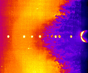
PLS images provide instantaneous views of the XSWBLI structures. The PLS images were acquired at 10 Hz, and the 1 mm thick laser sheet was parallel to and centred 1 mm from the surface of the plate. The field of view is  $97\ \textrm {mm} \times 97\ \textrm {mm}$. Figure 5 is a PLS image with located at $11.0d$ from the plate leading edge. The leading edge of the cylinder is barely visible on the right-hand side of the image, and the bright dots in a horizontal line are the laser reflecting off of the flush-mounted pressure transducers. The flow is from left to right. Between the dots on the left is a faint, arc-shaped gradient where the image becomes lighter. This location is marked as ‘upstream influence’ (UI) and the reason for the increase in brightness is an increase in number density of the ethanol fog particles across a weak shock. This shock occurs at $l/d = -6.4$ on the centreline in this image, but it should be noted that the laser sheet is 1 mm off of the surface of the plate, and because the shock structures occur at small angles the origin of this shock is farther upstream. Based on the PLS image, there does not appear to be any evidence of separated flow at this location, although a separation bubble could very well exist beneath the laser sheet. Near $l/d = -5$ there is a decrease in the intensity that is caused by a decrease in the number density of fog particles, which suggests an expansion wave exists near the end of the plateau region. Farther downstream, at $l/d = -3.6$, there is a very dark region that represents the slower, warmer fluid of a boundary layer or separated shear layer owing to the increased temperature in this region. The upstream edge of this darker flow has many finger-like structures. Turbulent interactions are known to exhibit Görtler vortices in the shear layer due to the concave streamline curvature associated with flow separation (Priebe et al. Reference Priebe, Tu, Rowley and Martin2016). It is probable that the structures observed here are due to the same mechanism. The shape of the dark region is also consistent with that of previous studies (Young et al. Reference Young, Kaufman and Korkegi1968; Kaufman et al. Reference Kaufman, Korkegi and Morton1972; Hood Reference Hood2003) that observed that the separation line for transitional interactions did not have a constant radius of curvature, which is different from both laminar and turbulent interactions. In this PLS image there appears to be a similar inflection point in the outboard region on both sides of the cylinder.

Figure 5. PLS image of transitional interaction for cylinder located  $11.0d$ upstream of the plate leading edge. UI occurs at $l/d = -6.4$, and the separation begins at $l/d = -3.6$.
The PLS images are consistent with the pressure data in that they show both the region of upstream influence and the separated region. The upstream influence in the PLS images is smaller than that inferred from both the pressure measurements (shown later), but this is consistent with the fact that the laser sheet is above the plate surface. The beginning of the dark structures is well upstream of the separation location inferred from the pressure data and schlieren imaging. This difference in location suggests that these finger-like structures might not be due to a fully separated region, but might be associated with a thickening boundary layer.
3.1.2. Schlieren imaging
Some caution is required when interpreting the schlieren results considering that this is a path-integrated technique. A representative image of a transitional interaction is presented in figure 6. In this figure the cylinder is located  $13.1d$ downstream of the plate leading edge. The inclined wave in the upper half of the image and the clearly defined vertical wave immediately upstream of the cylinder are the plate leading-edge shock and the steady cylinder bow shock, respectively. Oblique shock waves originate from two different locations in the interaction. The upstream influence wave is estimated via extrapolation to originate from $5.7d$ upstream of the cylinder leading edge, and is at approximately the same angle as the leading edge shock, $12.5^{\circ }$. This value is close to the Mach angle for Mach 4.92 edge flow, which is $11.7^{\circ }$. Using inviscid flow theory, this wave angle implies that the disturbance causing this upstream wave is generating a wave with a pressure ratio of approximately 1.15. Farther downstream there are multiple oblique shocks that coalesce at the triple point. These shocks originate from between $4.1d$ and $2.8d$ upstream of the cylinder. The downstream shocks are stronger and are at a higher angle than the upstream shock, meaning that the flow deflection that caused them is greater than that which caused the upstream shock. The presence of multiple shocks is consistent with the results of previous studies (Young et al. Reference Young, Kaufman and Korkegi1968; Hood Reference Hood2003; Combs et al. Reference Combs, Kreth, Schmisseur and Lash2018a,Reference Combs, Lash, Kreth and Schmisseurb). The location of the origin of the upstream shock is consistent with UI, which means that the retarded or weakly separated flow in the upstream region as inferred by PLS is the likely cause. Again, the line-of-sight integrated nature of schlieren imaging means that the waves could be occurring at different spanwise locations, but the consistency with previous results of other measurements suggests otherwise.

Figure 6. Representative spark schlieren image and schematic of transitional interaction with cylinder located  $13.1d$ upstream of the plate leading edge ( $Re_{X} = 7.3\times 10^{6}$).
3.1.3. Mean pressure profiles
The wall pressures were averaged to provide the mean pressure distribution along the centreline of the interaction. As previously mentioned, these measurements were taken with the cylinder located  $12.9d$ from the plate leading edge or $Re_{X} = 7.1 \times 10^{6}$.
Figure 7 shows the mean wall pressure under the interaction normalized by the nominal free-stream pressure vs the distance from the leading edge of the cylinder normalized by the cylinder diameter for this  $12.9d$ case. Furthermore, figure 7 presents the mean wall pressure at each location averaged over all of the runs where the cylinder was located $12.9d$ from the plate leading edge. The solid line is a moving spline trend line and has been added to make it easier to see the trend of the data. The uncertainty estimates shown for each location represent the 95 % confidence interval as calculated with the Student's $t$ distribution based on the data from the repeated runs, coupled with the uncertainty related to transducer error and calibration. For the majority of the transducer locations the measurements were only repeated twice (empty symbols), which causes the uncertainty to be relatively large (roughly 30 % higher than with three repeated measurements and over 50 % higher than with four repeated measurements, for example). At locations where the measurements were repeated more times the uncertainty is much lower, as shown by the points with filled symbols. It is believed that the uncertainty estimates for these locations provide a better estimate of the repeatability of the measurements than those where the measurements were only repeated twice. The $x$-axis includes a to-scale schematic of the plate and cylinder for reference. The initial UI of the SWBLI as determined by disturbances in the wall-pressure measurements occurs between 8 and 9 diameters upstream of the cylinder, whereas the literature shows that UI for a turbulent interaction is approximately $3d$ (Westkaemper Reference Westkaemper1968). Laminar interactions have a UI of up to $12d$ (Hung & Clauss Reference Hung and Clauss1980), indicating that this cylinder location is likely generating a transitional interaction. However, it is possible that the upstream influence location is limited by the upstream leading edge of the plate given that the cylinder is only $12d$ downstream of the leading edge. Beginning at UI, the mean wall pressure rises until approximately $l/d = -6.5$, at which point it reaches a plateau until near $l/d = -4$. The plateau pressure level is approximately $1.25P_{\infty }$, which is approximately 7 % lower than the value of $1.34P_{\infty }$ predicted by Hill's correlation for laminar plateau pressure as a function of $M_{\infty }$ and $Re_{X_{sep}}$ (Hill Reference Hill1967)
 \begin{equation} \frac{P}{P_{\infty}}=1+1.218M_{\infty}^{2}\left[\left(M_{\infty}^{2} -1\right)Re_{X_{sep}}\right]^{-{1}/{4}}. \end{equation}
Figure 7. Normalized mean wall pressure for the  $12.9d$ cylinder position as a function of normalized distance upstream of cylinder leading edge with uncertainty estimates based on the Student's $t$ distribution. To-scale plate and cylinder schematic on $x$-axis for reference.
This correlation was not derived from transitional results, but it makes sense that if there was a plateau region in a transitional interaction the pressure would be less than this correlation predicts since  $Re_{X_{sep}}$ would be larger. The mean pressure then increases to a maximum of $1.75P_{\infty }$ at $l/d = -2.5$. This is followed by a decrease in pressure to $1.5P_{\infty }$ at $l/d = -2$. The mean pressure at the cylinder root was found to be an order of magnitude higher than the free stream, with a value of $11.2P_{\infty }$.
The general shape of the mean wall-pressure profile is qualitatively consistent with the description of the compression-ramp-induced transitional interactions by early investigators (Chapman et al. Reference Chapman, Kuehn and Larson1958; Needham & Stollery Reference Needham and Stollery1966; Roberts Reference Roberts1970), which showed an initial rise to a plateau and then a subsequent increase in pressure up to the flow reattachment on the ramp face. The main difference here is that the subsequent rise that occurred on the ramp face is occurring a considerable distance upstream of the cylinder. This qualitative comparison to the previous studies of transitional interactions is useful but limited due to the differences in shock generating geometry. An interesting observation is that the mean pressure profile is very nearly a stitching of an upstream laminar cylinder-induced interaction to a downstream turbulent interaction. Centreline pressure profiles for laminar interactions measured by Young et al. (Reference Young, Kaufman and Korkegi1968) were not as extensive in the streamwise direction as those of the current study, but the plateau pressure they measured was also very close (within 2 %) to that predicted by (3.1). Young et al. (Reference Young, Kaufman and Korkegi1968) showed the wall pressure in the laminar case to decrease after reaching the value predicted by the free-interaction hypothesis, but the transitional profile of the current study has a second region of increasing mean pressure after the plateau region. The mean profile from  $l/d = -4$ to the fin root bears a qualitative resemblance to measurements of a fully turbulent interaction as measured by Brusniak (Reference Brusniak1994). The increase in the mean wall pressure for the turbulent interaction is relatively abrupt, but the compression in the transitional interaction is likely more spread out, similar to what is seen in lower $Re$ turbulent interactions (Ringuette, Wu & Martin Reference Ringuette, Wu and Martin2008). Additionally, the turbulent profile does not have a plateau, and instead peaks near $l/d = -2$. Figure 8 shows mean wall-pressure profiles for model laminar and turbulent interactions derived from Young et al. (Reference Young, Kaufman and Korkegi1968) and Brusniak (Reference Brusniak1994), respectively. The green dashed line is a composite of these two model profiles and the data from the $12.9d$ cylinder position are plotted for comparison. The green line was produced by initially plotting a straight line to approximately match the initial undisturbed conditions, followed by a line matching the theoretical laminar profile from the UI location to the approximate separated flow location, at which point the theoretical turbulent profile was used to the cylinder root. The pressure profile in the downstream region of the transitional interaction is slightly stretched in the streamwise direction relative to that of a fully turbulent interaction, which is consistent with previous measurements (Kaufman et al. Reference Kaufman, Korkegi and Morton1972). Compared with the work of Brusniak (Reference Brusniak1994), the normalized pressure of the current study is approximately half that of a turbulent interaction, except at the root of the cylinder, where the values are of the same order – but still less than – the inviscid value of 29 $P_{\infty }$. The transitional interaction therefore has a weaker compression upstream of the cylinder, whereas similar pressure levels are reached at the cylinder root.

Figure 8. Composite mean wall-pressure profiles for model laminar and turbulent interaction derived from Young et al. (Reference Young, Kaufman and Korkegi1968) and Brusniak (Reference Brusniak1994), respectively. Mean wall-pressure measurements for transitional interaction with the cylinder located  $12.9d$ from the plate leading edge plotted for comparison.
3.1.4. Global flow field
A conceptual model of the flow field of cylinder-induced transitional SWBLIs is shown in figure 3. This model was developed through a synthesis of the results presented here. The upstream influence, as evidenced by the initial rise in the mean wall pressure, is located between  $-8d$ and $-6d$. The region immediately behind UI is the plateau region. It is not clear whether this region is simply a region of retarded flow or if there is a separation bubble present. No evidence of separation is seen in the PLS images, so if there is indeed separated flow in this region its height is less than 1 mm (or 0.67 boundary-layer thicknesses). Farther downstream at $-4.1d$, a comparison of the schlieren image and pressure profile (figure 9) shows that the downstream primary shock structure and sharp pressure rise appear to coincide with a region of separated flow or perhaps a thickening boundary layer. This also appears to correspond to a region where the finger-like structures begin in the PLS images, further suggesting this is representative of an enlarged boundary layer that is protruding through the laser sheet, although this interaction was recorded at a slightly different $x$-station. This feature generates a strong oblique shock, followed by expansion structures and corresponding pressure drop at approximately $-2.8d$. A closure shock is seen at approximately $-2.1d$ in the schlieren image that appears to correspond to another pressure rise in the mean pressure profile. It should be noted that features of the mean wall-pressure profile (e.g. the gradual rise in pressure downstream of the plateau region) might not be explained by the conceptual model in and of itself, but might be products of the inferred flow field coupled with the interaction unsteadiness. A comparison of these findings is also summarized in table 2. We should also note that while it is possible that the interaction exhibits bimodal behaviour where the features effectively switch between the structure of a laminar and turbulent interaction, we feel this is unlikely given the statistics provided in later sections and the recent work of Combs et al. (Reference Combs, Lash, Kreth and Schmisseur2018b, Reference Combs, Schmisseur, Bathel and Jones2019) that demonstrated for transitional interactions the probability density functions (p.d.f.s) of shock motion exhibit unimodal behaviour.

Figure 9. Comparison of pressure measurements and representative schlieren image. The top image is the mean wall-pressure profile with the cylinder located  $12.9d$ from the plate leading edge ( $Re_{x} = 7.1 \times 10^{6}$) and the lower image is a schlieren image with the cylinder at $13.1d$ ( $Re_{x} = 7.2 \times 10^{6}$).
Table 2. Comparison of flow structures observed with various measurement techniques.

3.2. Interaction dynamics
The objective of the second part of the study was to characterize the dynamics of the transitional interaction. High-frequency response pressure measurements were recorded on the wall underneath the transitional interaction with the cylinder located  $12.9d$ from the plate leading edge. Measurements were also recorded below the undisturbed boundary layer to provide a baseline comparison case. Basic statistical quantity profiles and time-series analyses of the interaction are presented. Error bars are provided to represent uncertainty estimates for the averaged quantities, using the same procedure described for figure 7.
The time-dependent character of the wall-pressure signals changes significantly throughout the streamwise extent of the interaction. The standard deviation of the pressure measurements gives a quantitative idea of the streamwise evolution of the pressure fluctuations. The centreline standard deviation distribution in figure 10(a) shows an initial increase at  $l/d = -8\text { to }{-}9$, followed by a more shallow rise to approximately $l/d = -5$. The profile then increases monotonically until $l/d = -1$. There is not nearly as much scatter in the data as that seen in the mean wall pressure because the mean has been subtracted out. One region where there appears to be more scatter is between $l/d = -3\text { and }{-}4$. According to the mean wall-pressure profile, this location is just after the plateau region, where the profile begins to assume the character of a turbulent interaction. At the corresponding location in a turbulent interaction, the standard deviation profile has been shown to have two local maxima, as shown by Brusniak (Reference Brusniak1994). The standard deviation does reach a local maximum at $l/d = -3.83\text { and }{-}3.17$, but given the relatively small scale of this structure in the $x$-direction, the resolution of the measurements in the current study is not sufficient to say definitively that these maxima are present and not just a result of scatter. The normalized magnitude of the standard deviation is an order of magnitude larger than that of the undisturbed boundary layer, but downstream of the plateau region is at least a factor of two smaller than that of a turbulent interaction (Brusniak & Dolling Reference Brusniak and Dolling1994) but comparable to similar measurements of cylinder-induced transitional interactions (Combs et al. Reference Combs, Lash, Kreth and Schmisseur2018b). Even near the root of the cylinder the variance of the pressure for the transitional interaction is significantly less than that of a turbulent one (Brusniak & Dolling Reference Brusniak and Dolling1994).

Figure 10. (a) Normalized standard deviation of the centreline wall-pressure measurements as a function of normalized distance upstream of cylinder leading edge, (b) streamwise skewness ( $\alpha _{3}$) profile and (c) streamwise kurtosis ( $\alpha _{4}$) profile for the cylinder located $12.9d$ from the plate leading edge.
The skewness ( $\alpha _{3}$) profile along the centreline is shown in figure 10(b). The skewness is a measure of the direction in which the pressure p.d.f. is weighted, with $\alpha _{3} > 0$ indicating a distribution biased towards lower pressures and vice versa. For the length of the interaction, $\alpha _{3}$ is, for the most part, greater than zero. This means that at every point the p.d.f. is weighted towards lower pressures and has a longer tail on the higher pressure side. The skewness is at a maximum just downstream of UI, and decreases to a near constant level in the plateau region. At $l/d = -3.83$, $\alpha _{3}$ begins to increase until it reaches a local maximum at $l/d = -1.17$.
Figure 10(c) shows the kurtosis ( $\alpha _{4}$) profile along the plate centreline. The kurtosis gives an idea of the peakedness of the profile – in other words the width or length of the tails of the p.d.f. For a normal distribution $\alpha _{4} = 3$, with a higher value indicating that the distribution is more peaked with wider tails (i.e. the data have more outlying points than a normal distribution). The kurtosis profile has a maximum 1 $d$ upstream of the maximum in $\alpha _{3}$. The kurtosis then decreases to that of a normal distribution at $l/d = -7.5$, and remains at that level until $l/d = -3.83$. Between $l/d = -3.83\text { and }{-}1$, the kurtosis is approximately 3.5 and appears fairly constant within the uncertainty.
These profiles provide a basic description of the dynamics of the interaction. At  $l/d = -8.83$, the kurtosis is very high, but the skewness is very close to zero. This implies that there are data points that are very much outliers, but that they occur infrequently enough that the skewness – and also the standard deviation – are basically unaffected. This location corresponds to a point at the far upstream end of the interaction (or potentially the most upstream extent of the interaction region or beyond, where a diminishing part of the upstream pressure rise passed upstream through the subsonic portion of the boundary layer is detected) that sees the pressure rise due to the interaction very infrequently. This is very much like the peak at the upstream edge of the intermittent region observed by Dolling & Murphy (Reference Dolling and Murphy1983) for a compression ramp interaction at Mach 3. Just downstream, at $l/d = -8.17$, the skewness is very high, but the kurtosis has decreased. This is akin to a point in the upstream portion of the intermittent region of a turbulent interaction, again similar to what was measured by Dolling & Murphy (Reference Dolling and Murphy1983). The pressure is mostly at a lower, undisturbed value, but the higher downstream pressure sweeps over this region fairly often. Thus the p.d.f. is very much weighted towards the lower pressure, but the peakedness is still near normal. In the plateau region the skewness is near zero, and the kurtosis is 3, also suggesting normally distributed fluctuations. Between $l/d = -4 \text { and }{-}1$, the kurtosis is slightly higher than 3, and the skewness steadily increases. This is similar to what occurs downstream of the intermittent region in a turbulent interaction, where both skewness and kurtosis increase (Dolling & Murphy Reference Dolling and Murphy1983). These statistics suggest an unsteadiness in which the whole interaction expands and contracts, similar to the unsteadiness mechanism of turbulent interactions described by Brusniak & Dolling (Reference Brusniak and Dolling1994), which they called the ‘global flow field hypothesis’.
Figure 11 shows the power spectra presented in a way that emphasizes the streamwise evolution of the frequency content of the interaction. In the upstream portion of the interaction (from  $l/d = -8\text { to }{-}4$) there is a clear bump centred at 2 kHz. To aid comparisons with the existing literature, the data are also provided in terms of Strouhal number. Here, two different Strouhal number scalings are presented: (i) Strouhal number based on turbulent separation length $L$, where $St_{L} = fL/U$ with $U$ representing the free-stream velocity and $f$ representing frequency and (ii) Strouhal number based on boundary-layer height $\delta$, where $St_{\delta } = f\delta /U$. Consistent with the review of Clemens & Narayanaswamy (Reference Clemens and Narayanaswamy2014) the turbulent separation length scale has been defined as the difference between the upstream turbulent separation location and the downstream reattachment point, which is approximately $3d$ in the present study. As anticipated based on previous investigations of cylinder-induced interactions (Clemens & Narayanaswamy Reference Clemens and Narayanaswamy2014; Combs et al. Reference Combs, Lash, Kreth and Schmisseur2018b; Lindörfer et al. Reference Lindörfer, Combs, Kreth, Bond and Schmisseur2020), the energy bump is located primarily between $St_{L} = 0.05\text { and }0.2$, indicative of unsteadiness at low frequencies relative to the separation scale. The frequency scaling is approximately one order of magnitude lower relative to boundary-layer scaling, and it is possible that the oscillation frequency is not dependent on the incoming boundary-layer scale for this flow configuration based on the work of Lindörfer et al. (Reference Lindörfer, Combs, Kreth, Bond and Schmisseur2020). At $l/d = -4$, the energy shifts to a more broadband distribution at much higher frequencies. This is consistent with a region of reattached turbulent flow. In the downstream region, the energy alternates between this broadband, high-frequency content and a more peaked low-frequency content. The low-frequency fluctuations for both regions occur at the same frequency, suggesting that there may be a relationship between the two. Effectively, the frequency of oscillation in this non-turbulent region seems to exhibit an $St_L$ that is consistent with the downstream turbulent separated flow, which seems to suggest a coupling between the upstream and downstream unsteady motions.

Figure 11. Streamwise variation of normalized pressure power spectral density as a function of frequency for a cylinder located  $12.9d$ from the plate leading edge. Plotted with a schematic of the interaction for reference.
To examine the relationship between the energy contained at certain frequencies, the mean-squared coherence function was calculated for wall-pressure measurements at a number of different locations within the interaction. The coherence function ( $\gamma _{xy}^{2}$) is a measure of the degree of linearity between the energy contained at a given frequency for two signals $x$ and $y$, where $x$ is the reference signal. The relationship between the two signals is purely linear if $\gamma _{xy}^{2}$ = 1. Figure 12 shows the coherence as a function of frequency for the majority of the streamwise extent of the interaction. The reference transducer for these coherence functions is located at $l/d = -7.50$, which is near the centre of the initial pressure rise. For $l/d = -6.17$, $\gamma _{xy}^{2}$ is very high for the frequencies below 3 kHz, with a peak at 1–2 kHz. For $l/d = -4.83$, $\gamma _{xy}^{2}$ is still high for these lower frequencies. The coherence function between the reference transducer and $l/d = -3.50$ is relatively low across the spectrum. This is interesting because this suggests that the plateau region and the region of reattached flow are not linearly related. Even more interesting is that for $l/d = -2.17$ there is once again strong coherence between the two signals at frequencies from 1 to 2 kHz. This means that the fluctuations within the plateau region are linearly related to each other and also to the low-frequency fluctuations between $l/d = -2.5\text { and }{-}1.83$.

Figure 12. (a) Schematic of locations for coherence function calculations, (b) mean-square coherence as a function of frequency for cylinder located  $12.9d$ from the plate leading edge. The reference transducer is located at $l/d = -7.50$.
Farther downstream the coherence function is quite different. Figure 13 shows the coherence function for pressure measurements collected downstream of the plateau region, with the reference transducer located at  $l/d = -5.17$, which is near the downstream end of the plateau region. Both $l/d = -4.83 \text { and }{-}4.50$ have coherence peaks at 2 kHz, but, unlike the measurements in the plateau region, the measurements remain coherent until almost 10 kHz. The coherence at 2 kHz has decreased slightly for $l/d = -3.83$, but the higher-frequency coherence is much lower. The coherence between the reference transducer and $l/d = -3.17$, which is underneath the reattached flow, is low across the entire measured frequency range.

Figure 13. (a) Schematic of locations for coherence function calculations, (b) mean-square coherence as a function of frequency downstream of the plateau region for the cylinder located  $12.9d$ from the plate leading edge. The reference transducer is located at $l/d = -5.17$.
The temporal relationship between the pressure fluctuations can be inferred from cross-correlations. The cross-correlation shows at what time lag the similarity between two signals is maximized. A positive correlation at a positive (negative) time lag corresponds to a downstream pressure fluctuation preceding (preceded by) an upstream fluctuation of the same sign. Figure 14 shows the cross-correlations between wall-pressure measurements at streamwise locations for the majority of the interaction. The reference location is  $l/d = -7.50$, near the upstream edge of the plateau region. The correlation for $l/d = -6.17$ is relatively high with a positive peak at $81\ \mathrm {\mu }\textrm {s}$. At $l/d = -4.83\text { and }{-}3.50$ the correlation peak has decreased but is still positive at $t = 168\text { and }185\ \mathrm {\mu }\textrm {s}$, respectively. In the downstream region, at $l/d = -2.17$, the correlation has a negative peak at $t = 137\ \mathrm {\mu }\textrm {s}$. This location is in the downstream region where the fluctuations were linearly related to those in the plateau region. Unlike cross-correlations in turbulent interactions, these data do not show the sharp peak that is associated with convection of structures through the interaction because the pressure fluctuations in the upstream boundary layer occur at a very high frequency and are not resolved. These cross-correlation results suggest that the fluctuations originate between $l/d = -4.83\text { and }{-}3.5$.

Figure 14. (a) Schematic of locations for cross-correlation calculations, (b) cross-correlations through interaction for cylinder located  $12.9d$ from the plate leading edge. Reference transducer is located at $l/d = -7.50$.
To further examine this behaviour, cross-correlations were calculated upstream and downstream of this fluctuation origin. Figure 15 shows two cross correlations: between  $l/d = -6.17\text { and }{-}4.83$, and between $l/d = -3.50\text { and }{-}2.17$. The results are consistent with the earlier interpretation as the pressure fluctuations at $l/d = -4.83\text { and }{-}3.50$ precede those at $-6.17$ and $-2.17$, meaning that the fluctuations propagate upstream in the upstream region. The propagation velocity ( $U_{\Delta p}$) of the upstream disturbance can be calculated based on the peak in the correlation and the known distance between the measurement stations. In the upstream direction the disturbance propagates at $0.23U_{\infty }$, similar to the results of Combs et al. (Reference Combs, Lash, Kreth and Schmisseur2018b) and Larchevêque (Reference Larchevêque2016) where the upstream propagation speed ranged from approximately 10 %–20 % of $U_{\infty }$. In the recent work of (Threadgill, Little & Wernz Reference Threadgill, Little and Wernz2019) the ‘slow’ propagation was found to occur at a velocity of $0.33U_{\infty }$ while the ‘fast’ disturbance propagation occurred with a velocity of $0.69U_{\infty }$, with a group propagation speed of $0.18U_{\infty }$. Overall, the computed propagation velocity is consistent with a reattached downstream region and separated flow in the upstream region.

Figure 15. (a) Schematic of locations for cross-correlation calculations, (b) cross-correlations of pressure measurements between pairs of transducers on either side of the inferred fluctuation origin for cylinder located  $12.9d$ from the plate leading edge.
A closer look at the correlations of measurements in the plateau region is provided in figure 16, and shows cross-correlations for successive transducer pairs in the plateau region. Considering that the fluctuations are propagating upstream, the peaks in the correlation can again be used to calculate the fluctuation propagation velocity between the measurement locations. It was found that the propagation velocity ( $U_{\Delta P}$) decreases as the fluctuations move upstream and figure 17 shows $U_{\Delta P}$ as a function of normalized distance from the cylinder. As seen in the figure, the propagation velocity decreases proportionally to the square of the distance from the cylinder. However, we should note that these results should be interpreted with caution considering that correlations obtained from such measurements can exhibit secondary peaks because of concomitant physics occurring over distinct frequency bands. As seen in the power and cross-spectra, there are (at least) two distinct main unsteady physics associated with distinct frequency bands and it is likely that at some locations these physics occur simultaneously. This therefore has the potential to complicate any conclusions drawn from the two-point correlations in the present work.

Figure 16. (a) Schematic of locations for cross-correlation calculations, (b) cross-correlations between successive transducers in the plateau region for cylinder located  $12.9d$ from the plate leading edge.

Figure 17. Fluctuation propagation velocity in the plateau region as a function of normalized distance from the cylinder leading edge. Positive  $U_{\Delta P}$ corresponds to upstream propagation. The $x$-axis values correspond to averaged locations of the two sensors used in each correlation.
4. Summary and conclusions
Shock-wave/transitional boundary-layer interactions generated by a circular cylinder mounted on a flat plate were studied at Mach 5. The current manuscript focuses on measurements recorded for a cylinder position corresponding to an  $Re_{X}$ value of $7.1 \times 10^{6}$ where the incoming boundary layer was transitional. The study consisted of two parts: a description of the global flow field of the interaction and a detailed analysis of the interaction unsteadiness.
Mean wall-pressure measurements in the streamwise direction on centreline showed that the upstream influence location for these interactions occurred approximately 8.5 $d$ upstream of the cylinder leading edge. The streamwise mean wall-pressure profile had an initial rise in pressure at UI, followed by an approximately $3d$ long plateau region. In the plateau region the normalized mean wall pressure was found to be lower but within 10 % of the value predicted for the plateau pressure of a purely laminar interaction by the free-interaction hypothesis. At approximately $4d$ upstream of the cylinder, the mean pressure begins to rise again, reaching a local maximum near $2d$ upstream of the cylinder and then decreases to a local minimum near $0.5d$ upstream of the cylinder before increasing by an order of magnitude in the immediate vicinity of the cylinder root. The pressure profile resembles a composite of a laminar and turbulent interaction.
PLS and schlieren results also suggest that the transitional interaction exhibits the characteristics of a laminar interaction in the upstream region and a turbulent interaction in the downstream region. The PLS showed an increase in the number density of fog particles that implies a weak shock at UI. Immediately downstream of the plateau region, the PLS shows a slightly darker region which is believed to be caused by an expansion on the aft end of the upstream separation bubble. Downstream of the expansion the PLS shows darker structures protruding through the laser sheet, which are caused by the growth of the reattached boundary layer. The flow visualization results also suggest that the downstream region is nearly insensitive to changes in  $Re_{X}$, which is very similar to the behaviour of purely turbulent interactions. Schlieren images agree well with this flow field description, as they show a weaker upstream shock originating from UI and a stronger downstream shock originating from the downstream end of the plateau region.
Statistics of the wall-pressure measurements suggest that the interaction unsteadiness is similar to the ‘global flow field hypothesis’ proposed by Brusniak & Dolling (Reference Brusniak and Dolling1994). The pressure power spectra indicate that large-scale motion occurs at approximately  $St_{L} = 0.05\text {--}0.2$, indicative of unsteadiness at low frequencies relative to the separation scale and consistent with previous investigations of cylinder-induced interactions (Clemens & Narayanaswamy Reference Clemens and Narayanaswamy2014; Combs et al. Reference Combs, Lash, Kreth and Schmisseur2018b; Lindörfer et al. Reference Lindörfer, Combs, Kreth, Bond and Schmisseur2020). Fluctuations within the plateau region are very coherent, and cross-correlations in this region show that the fluctuations propagate upstream at a velocity that decreases quadratically with distance from the leading edge of the cylinder. Coherence function and cross-correlation results support the assertion inferred from PLS that the upstream region is a separated flow and not just a retarded region. Immediately downstream of the plateau region is a region of relatively high-frequency broadband fluctuations, which is consistent with the interpretation from the PLS images of a reattached flow. Cross-correlations from transducer pairs straddling the downstream end of the plateau region indicate that the source of fluctuations is located at the downstream end of the plateau region/reattachment location, which suggests that the motion of this location might be driving the unsteadiness in both the upstream and downstream separated flow.
Acknowledgements
The views and conclusions contained herein are those of the authors and should not be interpreted as necessarily representing the official policies or endorsements, either expressed or implied, of the Air Force Office of Scientific Research or the U.S. Government. The authors would also like to thank Dr B. Ganipathisubramani, Dr J. Wagner, Dr M. Gamba and A. Valdivia for their help with the set-up and execution of experiments.
Funding
This work was sponsored (in part) by the Air Force Office of Scientific Research, USAF, under grant/contract number FA9550-04-1-0112. Additional support was provided to co-author Combs by AFOSR under grant/contract number FA9550-20-1-0190 and by NASA grant 80NSSC19M0194.
Declaration of interests
The authors report no conflict of interest.


 Open access