


1. Introduction
The mechanical aspects of fish locomotion, shaped by $500\times 10^6$
years of evolution, have fascinated scientists for more than a century (Shadwick & Lauder Reference Shadwick and Lauder2006). Elucidating the physical principles underlying the efficiency of these swimmers is the focus of recent studies aimed at advancing biologically inspired underwater robotic vehicles (Kern & Koumoutsakos Reference Kern and Koumoutsakos2006; Tytell et al. Reference Tytell, Hsu, Williams, Cohen and Fauci2010; Raj & Thakur Reference Raj and Thakur2016; Khalid et al. Reference Khalid, Wang, Akhtar, Dong, Liu and Hemmati2021b
). Moreover, uncovering the principles utilised by fish to enhance their swimming performance can inspire novel flow control techniques (Akbarzadeh & Borazjani Reference Akbarzadeh and Borazjani2019b
, Reference Akbarzadeh and Borazjani2020) for improving force generation in engineering applications. Despite recent studies on propulsive efficiency, manoeuvrability and fast starts in fish, understanding the physical mechanisms for different species is still in its early stages (Fish Reference Fish2020). Scaling analysis can help identify the dominant propulsion mechanisms and establish rule-of-thumb principles.
$500\times 10^6$
years of evolution, have fascinated scientists for more than a century (Shadwick & Lauder Reference Shadwick and Lauder2006). Elucidating the physical principles underlying the efficiency of these swimmers is the focus of recent studies aimed at advancing biologically inspired underwater robotic vehicles (Kern & Koumoutsakos Reference Kern and Koumoutsakos2006; Tytell et al. Reference Tytell, Hsu, Williams, Cohen and Fauci2010; Raj & Thakur Reference Raj and Thakur2016; Khalid et al. Reference Khalid, Wang, Akhtar, Dong, Liu and Hemmati2021b
). Moreover, uncovering the principles utilised by fish to enhance their swimming performance can inspire novel flow control techniques (Akbarzadeh & Borazjani Reference Akbarzadeh and Borazjani2019b
, Reference Akbarzadeh and Borazjani2020) for improving force generation in engineering applications. Despite recent studies on propulsive efficiency, manoeuvrability and fast starts in fish, understanding the physical mechanisms for different species is still in its early stages (Fish Reference Fish2020). Scaling analysis can help identify the dominant propulsion mechanisms and establish rule-of-thumb principles.
Numerous studies have been conducted to explain how the unique kinematics and morphology of fish enable them to achieve remarkable efficiency and agility across different body/caudal fin locomotion modes including anguilliform (Tytell Reference Tytell2004; Tytell & Lauder Reference Tytell and Lauder2004; Kern & Koumoutsakos Reference Kern and Koumoutsakos2006; Borazjani & Sotiropoulos Reference Borazjani and Sotiropoulos2009; Khalid et al. Reference Khalid, Wang, Akhtar, Dong, Liu and Hemmati2021b ), carangiform (Borazjani & Sotiropoulos Reference Borazjani and Sotiropoulos2008; Liu et al. Reference Liu, Ren, Dong, Akanyeti, Liao and Lauder2017; Lucas et al. Reference Lucas, Lauder and Tytell2020; Khalid et al. Reference Khalid, Wang, Akhtar, Dong, Liu and Hemmati2021a ), subcarangiform (Li et al. Reference Li, Ravi, Xie and Couzin2021) and thunniform (Hu et al. Reference Hu, Liang and Wang2015; Zhang et al. Reference Zhang, Sung and Huang2020). These locomotion modes and morphologies have evolved to meet the biological needs of each species. Unlike thunniform and carangiform fast swimmers, in which lateral undulation is limited to the posterior part of the body and a lunate-shaped caudal fin plays a crucial role in thrust generation (Sfakiotakis et al. Reference Sfakiotakis, Lane and Davies1999; Borazjani & Sotiropoulos Reference Borazjani and Sotiropoulos2010; Borazjani & Daghooghi Reference Borazjani and Daghooghi2013; Khalid et al. Reference Khalid, Wang, Akhtar, Dong, Liu and Hemmati2021a ), anguilliform swimmers pass a travelling wave from head to tail with all undulating segments contributing to the thrust force (Tytell & Lauder Reference Tytell and Lauder2004). Carangiform swimmers like mackerels are capable of high-speed swimming and are adapted for sustained cruising over long distances, while anguilliform swimmers, like eels, are generally slower but are more manoeuvrable in confined spaces (Sfakiotakis et al. Reference Sfakiotakis, Lane and Davies1999). Anguilliform kinematics and morphology have been less frequently adopted in bioinspired underwater robots, compared with thunniform or carangiform ones (Fish Reference Fish2020), likely because they are perceived as slower and less efficient (Blake Reference Blake2004). However, recent studies show that anguilliform swimmers are more efficient than carangiform swimmers at low Reynolds number regimes (Borazjani & Sotiropoulos Reference Borazjani and Sotiropoulos2010; Daghooghi & Borazjani Reference Daghooghi and Borazjani2016). An observational study by van Ginneken et al. (Reference van, Vincent, Erik, Ulrike, Booms, Eding, Verreth and van den Thillart2005) shows that the European eel Anguilla anguilla is capable of long-distance migration (5000–6000 km), highlighting the swimming efficiency of eels.
A key parameter in analysing the hydrodynamic performance of swimmers, in terms of swimming efficiency and cruising speed, is the thrust force (Lighthill Reference Lighthill1960; Borazjani & Sotiropoulos Reference Borazjani and Sotiropoulos2008). From a classical point of view, the mechanisms of thrust force generation in body–caudal fin propulsion can be broadly categorised into resistive force, reactive force and lift-based mechanisms (Webb & Weihs Reference Webb and Weihs1986). In the resistive force model, first suggested by Taylor (Reference Taylor1952), viscous friction force on the body generates a component along the swimming direction at low Reynolds numbers (Piñeirua et al. Reference Piñeirua, Godoy-Diana and Thiria2015). In the reactive model, independently formulated by Wu (Reference Wu1961) and Lighthill (Reference Lighthill1960), inertial force is generated by momentum exchange due to fluid accelerated (added mass) away from the swimmer’s body at high Reynolds numbers (Borazjani & Sotiropoulos Reference Borazjani and Sotiropoulos2009; Khalid et al. Reference Khalid, Wang, Dong and Liu2020), see figure 1(a). The component of this force along the swimming direction contributes to the thrust force. In the lift-based force model, circulation generated around the fish’s tail produces a lift force (similar to an airfoil) which has a component along the swimming direction (Fish Reference Fish1994; Borazjani & Sotiropoulos Reference Borazjani and Sotiropoulos2010; Bottom II et al. Reference Bottom II, Borazjani, Blevins and Lauder2016), see figure 1(b). Fish employing this mechanism exhibit fewer body undulations and rely more on tail oscillations for propulsion.
While both reactive and lift-based models are used to explain mechanisms of thrust generation at high Reynolds numbers (Chen et al. Reference Chen, Friesen and Iwasaki2011; Eloy Reference Eloy2012; Khalid et al. Reference Khalid, Wang, Dong and Liu2020), any force on a swimmer’s body ultimately results from pressure and shear stress multiplied by area element, and integrated over its surface (Daghooghi & Borazjani Reference Daghooghi and Borazjani2015, Reference Daghooghi and Borazjani2016). According to the reactive-force theory (Lighthill Reference Lighthill1960), the motion of a body segment in a fluid accelerates the adjacent fluid creating a high pressure on one side and a low pressure on the other – see Appendix A for a simple example of the pressure distribution over a cylinder accelerating in an ideal fluid. On the other hand, according to the lift-based mechanism, circulation around the tail induces a pressure difference across the tail, which depends on the angle of attack (AoA) formed by the tail’s airfoil shape with the incoming flow. In other words, pressure difference across the swimmer’s body and fin can be attributed to the added-mass and/or circulation (AoA) mechanisms. This study investigates if the observed trends in pressure variation with swimming speed and body kinematics scale with the fluid acceleration, as predicted by the theory (Appendix A), and/or the lift-based force (AoA).
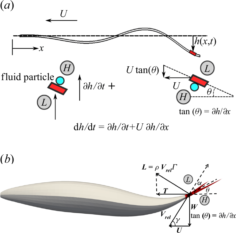
Figure 1. (a) The lateral displacement of body $h(x,t)$
accelerates adjacent fluid particles to velocity
$h(x,t)$
accelerates adjacent fluid particles to velocity $w=\textrm {d} h/\textrm {d}t$
, according to the slender body theory. This acceleration results from both the lateral velocity of the body
$w=\textrm {d} h/\textrm {d}t$
, according to the slender body theory. This acceleration results from both the lateral velocity of the body $W=\partial h/ \partial t$
and the angle of body against the swimming direction (
$W=\partial h/ \partial t$
and the angle of body against the swimming direction ( $U \partial h/\partial x$
). (b) The circulation (
$U \partial h/\partial x$
). (b) The circulation ( $\Gamma$
) is created due to flow passes over the tail (shown in red), causes a pressure difference across the tail. This pressure difference generates a lift force (
$\Gamma$
) is created due to flow passes over the tail (shown in red), causes a pressure difference across the tail. This pressure difference generates a lift force ( $L$
), which has a component in the forward (thrust) direction. This lift-based force is proportional to the AoA
$L$
), which has a component in the forward (thrust) direction. This lift-based force is proportional to the AoA $\alpha$
, defined as the angle between the relative velocity and the body’s reference line. The angles
$\alpha$
, defined as the angle between the relative velocity and the body’s reference line. The angles $\theta$
and
$\theta$
and $\gamma$
represent the angle formed by the relative velocity and the slope of the body with the swimming direction, respectively. Here
$\gamma$
represent the angle formed by the relative velocity and the slope of the body with the swimming direction, respectively. Here ![]() and
and ![]() denote high and low pressure sides, respectively.
denote high and low pressure sides, respectively.
The reactive and lift-based theories ignore viscous forces and assumes that the flow remains irrotational and attached over the swimmer’s body. Indeed, numerical (Kern & Koumoutsakos Reference Kern and Koumoutsakos2006; Borazjani & Sotiropoulos Reference Borazjani and Sotiropoulos2009; Li et al. Reference Li, Müller, van Leeuwen and Liu2016) and experimental studies (Tytell & Lauder Reference Tytell and Lauder2004) have shown that the body undulation in the form of travelling waves keep the boundary layer attached on the surface of aquatic swimmers. The fluid in the boundary layer, however, is rotational. The rotation in fluid (vorticity) within the boundary layer over an undulating fish might be due to the shear or the rotation of the body. A scaling analysis is conducted to determine whether the vorticity within the boundary layer of anguilliform and carangiform swimmers scales with the shear rate or the swimmer’s body rotation.
The kinematics of body motion play a crucial role in the hydrodynamics of swimming, particularly in thrust generation. Body motion not only influences the magnitude of surface forces by creating pressure difference along the body but also determines the angle between these force and the swimming direction. Wu (Reference Wu1961) and Lighthill (Reference Lighthill1960), proposed a sufficient condition for undulatory kinematics to produce thrust. Specifically, Lighthill (Reference Lighthill1960) discussed conditions for efficient thrust in eels, recommending the passage of a travelling wave (and not a standing wave) using slender-body theory for deformable bodies. More recently, it has been shown that travelling waves outperform standing waves in reattaching the flow over a thick airfoil (Akbarzadeh & Borazjani Reference Akbarzadeh and Borazjani2020; Ogunka et al. Reference Ogunka, Akbarzadeh and Borazjani2023).
Constructing virtual models of a lamprey and a mackerel, we performed self-propelled, wall-resolved large-eddy simulations at realistic swimming conditions (Reynolds and Strouhal numbers) to visualise the pressure field around and on the body. To the best of our knowledge, aside from previous works (Daghooghi & Borazjani Reference Daghooghi and Borazjani2015; Bottom II et al. Reference Bottom II, Borazjani, Blevins and Lauder2016; Ogunka et al. Reference Ogunka, Daghooghi, Akbarzadeh and Borazjani2020), there are no other self-propelled simulations of aquatic swimmers conducted at realistic Reynolds numbers. Recent simulations (Tytell et al. Reference Tytell, Hsu, Williams, Cohen and Fauci2010; Gazzola et al. Reference Gazzola, Chatelain, van Rees and Koumoutsakos2011; Li et al. Reference Li, Müller, van Leeuwen and Liu2016; Khalid et al. Reference Khalid, Wang, Akhtar, Dong, Liu and Hemmati2021b ) have been conducted at lower Reynolds numbers and/or were not self-propelled. By simulating the lamprey and mackerel using experimentally measured travelling waves (Videler & Hess Reference Videler and Hess1984; Tytell & Lauder Reference Tytell and Lauder2004; Hultmark et al. Reference Hultmark, Leftwich and Smits2007), as well as a hypothetical lamprey with standing wave body undulations, we revisited classical reactive and lift-based force theories. This approach allowed us to identify the dominant propulsion mechanism for these swimmers by examining whether the pressure distribution on the body scales with that of reactive (added mass) or lift-based theories. Furthermore, by comparing the energetics of swimming using experimentally measured travelling wave kinematics with hypothetical standing wave kinematics, we investigated the conditions for efficient swimming. Additionally, we analysed the vorticity scaling in the boundary layer over the swimmers.
2. Methods and material
2.1. Flow solver
The governing equations for the fluid solver are continuity and incompressible Navier–Stokes equations in a non-inertial frame of reference moving with the fish to reduce the computational cost. In the non-inertial reference frame, the position of the fish’s centre of mass (COM) does not change within the computational domain, i.e. the fish COM does not move forwards in the computational domain similar to our previous work, but it adds additional terms to the governing equations (Borazjani & Sotiropoulos Reference Borazjani and Sotiropoulos2010; Daghooghi & Borazjani Reference Daghooghi and Borazjani2015, Reference Daghooghi and Borazjani2016). The non-dimensional governing equations in curvilinear coordinates $\xi ^i=\xi ^i(x,y,z)$
using tensor notation (
$\xi ^i=\xi ^i(x,y,z)$
using tensor notation ( $i,j,m,n=1,2,3$
) are as follows (Borazjani et al. Reference Borazjani, Ge, Le and Sotiropoulos2013; Hedayat et al. Reference Hedayat, Akbarzadeh and Borazjani2022):
$i,j,m,n=1,2,3$
) are as follows (Borazjani et al. Reference Borazjani, Ge, Le and Sotiropoulos2013; Hedayat et al. Reference Hedayat, Akbarzadeh and Borazjani2022):
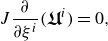 \begin{align} J\frac {\partial }{\partial \xi ^i} (\boldsymbol{\boldsymbol{\mathfrak {U}}}^i)=0 , \end{align}
 \begin{align} \frac {\partial \boldsymbol{\mathfrak {U}}^i}{\partial t}=\xi ^i_j\Big[-\frac {\partial }{\partial \xi ^n}((\boldsymbol{\mathfrak {U}}^n - \boldsymbol{\mathfrak {V}}^n) u_j)-\frac {\partial }{\partial \xi ^n}\left(\frac {\xi ^n_j}{J}p \right)+\frac {\partial }{\partial \xi ^n}\left(\frac {1}{Re_{\textit{eff}}}\frac {g^{nm}}{J}\frac {\partial {u_j}}{\partial \xi ^m} \right)\Big ] , \end{align}
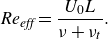 \begin{align} Re_{\textit{eff}}=\frac {U_0 L}{\nu +\nu _t} . \end{align}
Here, $L$
and
$L$
and $U_0$
are characteristic length (fish length) and velocity (nominal swimming speed);
$U_0$
are characteristic length (fish length) and velocity (nominal swimming speed); $x_i$
are the Cartesian position vector components non-dimensionalised by
$x_i$
are the Cartesian position vector components non-dimensionalised by $L$
;
$L$
; $t$
is time non-dimensionalised by
$t$
is time non-dimensionalised by $L/U_0$
;
$L/U_0$
; $\nu$
is the kinematic viscosity;
$\nu$
is the kinematic viscosity; $\rho$
is the fluid density;
$\rho$
is the fluid density; $u_i$
are the non-dimensional Cartesian velocity components (non-dimensionalised by
$u_i$
are the non-dimensional Cartesian velocity components (non-dimensionalised by $U_0$
);
$U_0$
); $J= \lvert (\xi ^1,\xi ^2,\xi ^3)/(x_1,x_2,x_3) \lvert$
is the determinant of the Jacobian of the transformation
$J= \lvert (\xi ^1,\xi ^2,\xi ^3)/(x_1,x_2,x_3) \lvert$
is the determinant of the Jacobian of the transformation $\xi ^j_m=\partial {\xi ^j}/ \partial {x_m}$
;
$\xi ^j_m=\partial {\xi ^j}/ \partial {x_m}$
; $g^{nm}$
is the contravariant metric of the transformation,
$g^{nm}$
is the contravariant metric of the transformation, $g^{nm}=\xi ^n_j \xi ^m_j$
;
$g^{nm}=\xi ^n_j \xi ^m_j$
; $p$
is the non-dimensional pressure, non-dimensionalised by
$p$
is the non-dimensional pressure, non-dimensionalised by $\rho U_0^2$
;
$\rho U_0^2$
; $\boldsymbol{\mathfrak {U}}^n=u_m\xi ^n_m/J$
and
$\boldsymbol{\mathfrak {U}}^n=u_m\xi ^n_m/J$
and $\boldsymbol{\mathfrak {V}}^n=v_m\xi ^n_m/J$
are the contravariant velocity of the fluid and grid, respectively, and
$\boldsymbol{\mathfrak {V}}^n=v_m\xi ^n_m/J$
are the contravariant velocity of the fluid and grid, respectively, and $\nu _t$
is the subgrid-scale turbulent viscosity, which is modelled using the dynamic subgrid-scale model (Germano et al. Reference Germano, Piomelli, Moin and Cabot1991). These equations are integrated in time using a second-order fractional step method consisting of a Newton–Krylov solver for the momentum equations and generalised minimal residual method solver enhanced with multigrid as a preconditioner for the Poisson pressure equation (Gilmanov & Sotiropoulos Reference Gilmanov and Sotiropoulos2005; Ge & Sotiropoulos Reference Ge and Sotiropoulos2007; Borazjani et al. Reference Borazjani, Ge and Sotiropoulos2008).
$\nu _t$
is the subgrid-scale turbulent viscosity, which is modelled using the dynamic subgrid-scale model (Germano et al. Reference Germano, Piomelli, Moin and Cabot1991). These equations are integrated in time using a second-order fractional step method consisting of a Newton–Krylov solver for the momentum equations and generalised minimal residual method solver enhanced with multigrid as a preconditioner for the Poisson pressure equation (Gilmanov & Sotiropoulos Reference Gilmanov and Sotiropoulos2005; Ge & Sotiropoulos Reference Ge and Sotiropoulos2007; Borazjani et al. Reference Borazjani, Ge and Sotiropoulos2008).
The solution of governing equations in the fluid domain requires inner and outer boundary conditions. The inner boundary condition is a no-slip condition between the fluid and the moving structure (virtual swimmer), and is handled with a sharp-interface immersed boundary method (Gilmanov & Sotiropoulos Reference Gilmanov and Sotiropoulos2005). In this method, grid nodes of the computational domain are classified as fluid nodes (outside of the immersed body), solid nodes (inside of the immersed body) and immersed nodes (immediate vicinity of the immersed body) using a ray-tracing algorithm (Borazjani et al. Reference Borazjani, Ge and Sotiropoulos2008). The velocity vector of immersed nodes is reconstructed along the normal direction of nearby surface mesh, using velocity vector of the moving surface nodes and has been shown to be second-order accurate (Gilmanov & Sotiropoulos Reference Gilmanov and Sotiropoulos2005).
The motion of the swimmer is a combination (superposition) of an undulatory mode (prescribed with respect to the non-inertial reference frame, attached to the fish), and a translational one, calculated through a partitioned fluid–structure interaction scheme (Borazjani et al. Reference Borazjani, Ge and Sotiropoulos2008). The body undulations are prescribed based on functions derived from experimental observations, see § 2.2. The undulatory motion of the swimmer creates a velocity and a pressure field in the fluid domain, and as well as a reacting stress (viscous and pressure) on its surface. By integrating this stress over the surface, the total exerted force on the swimmer’s surface is calculated (see (2.11)). The translational velocity of the swimmer’s COM is then obtained by integrating the total exerted force over time (Borazjani & Sotiropoulos Reference Borazjani and Sotiropoulos2008),
 \begin{align} C_m\frac {{\textrm{d}}U_i}{{\textrm{d}}t}=F_i , \end{align}
where $U_i=U_{s_i}/U_0$
is the non-dimensional swimming speed in the
$U_i=U_{s_i}/U_0$
is the non-dimensional swimming speed in the $i$
direction (
$i$
direction ( $U_{s_i}$
is the swimming velocity),
$U_{s_i}$
is the swimming velocity), $C_m=m/\rho L^3$
is the mass coefficient,
$C_m=m/\rho L^3$
is the mass coefficient, $m$
is the mass of the fish and
$m$
is the mass of the fish and $F_i$
is the dimensionless force (non-dimensionalised by
$F_i$
is the dimensionless force (non-dimensionalised by $\rho U_0^2 L^2$
) in the direction
$\rho U_0^2 L^2$
) in the direction $i$
. The swimmers are free to move in the streamwise and lateral directions. The non-dimensional swimming speed in the streamwise direction is denoted with
$i$
. The swimmers are free to move in the streamwise and lateral directions. The non-dimensional swimming speed in the streamwise direction is denoted with $U=U_s/U_0$
hereafter.
$U=U_s/U_0$
hereafter.
The flow solver and the structure solver are coupled through an implicit scheme (strong coupling) (Borazjani et al. Reference Borazjani, Ge and Sotiropoulos2008). In this fluid–structure interaction scheme, fluid dynamics and body motion equations are solved iteratively, until convergence is achieved (Borazjani & Daghooghi Reference Borazjani and Daghooghi2013; Daghooghi & Borazjani Reference Daghooghi and Borazjani2015, Reference Daghooghi and Borazjani2016).
To model turbulent flows under realistic conditions such as a Reynolds number of approximately 40 000 (Tytell Reference Tytell2004), three-dimensional (3-D) large-eddy simulations with a dynamic Smagorinsky subgrid-scale model (Kang et al. Reference Kang, Borazjani, Colby and Sotiropoulos2012; Akbarzadeh & Borazjani Reference Akbarzadeh and Borazjani2019a ) have been used. The curvilinear/immersed boundary solver has been successfully validated and applied to a wide range of problems, including self-propelled aquatic swimming simulations for a various range of Reynolds numbers (Borazjani & Sotiropoulos Reference Borazjani and Sotiropoulos2010; Borazjani & Daghooghi Reference Borazjani and Daghooghi2013; Daghooghi & Borazjani Reference Daghooghi and Borazjani2015, Reference Daghooghi and Borazjani2016; Bottom II et al. Reference Bottom II, Borazjani, Blevins and Lauder2016; Ogunka et al. Reference Ogunka, Daghooghi, Akbarzadeh and Borazjani2020).
2.2. Geometry and kinematics of swimmers
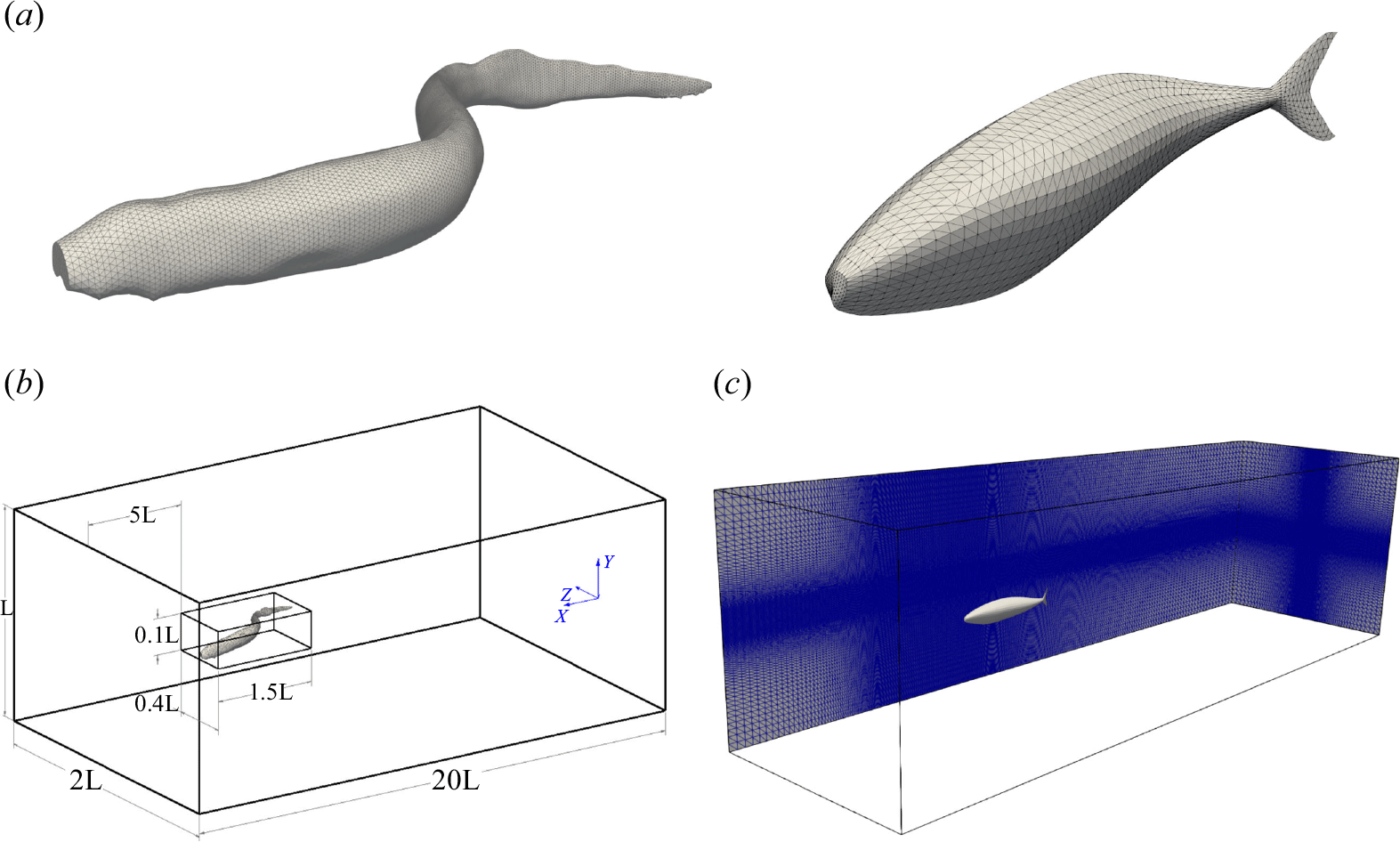
Figure 2. (a) Geometries of the lamprey and the mackerel are reconstructed from CT images. (b) The computational domain is a cuboid with a uniform high-resolution mesh around the swimmer. Dimensions are not to scale, refer to the detailed specifications for accurate dimensions. (c) The computational domain around the mackerel and mesh on two faces of the domain is visualised.
Figure 2(a) shows graphical projections of the virtual lamprey and mackerel, whose 3-D geometries were created from computed tomography (CT) images of an adult lamprey (Petromyzon marinus) and mackerel (Scomber scombrus), respectively. The anal and dorsal fins were removed from the model because the focus of this work is the pressure on the body of the swimmer. The constructed geometries are represented by a surface mesh with triangular elements, where each element is defined by three nodes. The instantaneous location of surface points relative to the non-inertial reference frame, attached to the fish, changes according to one of two prescribed modes of undulations. The first mode of motion is a backward travelling wave, which is obtained based on the experimental observations (Videler & Hess Reference Videler and Hess1984; Tytell & Lauder Reference Tytell and Lauder2004). We also considered a hypothetical standing wave with similar amplitude, frequency and wavelength for the lamprey. Considering swimming on the horizontal $x{-}z$
plane (figure 2), the non-dimensional lateral undulations with respect to the non-inertial reference frame are prescribed with time as follows:
$x{-}z$
plane (figure 2), the non-dimensional lateral undulations with respect to the non-inertial reference frame are prescribed with time as follows:
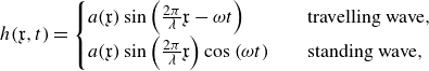 \begin{align} h(\mathfrak x,t) = \begin{cases} a(\mathfrak x)\sin \left ( \frac {2\pi }{\lambda } \mathfrak x- \omega t\right ) & \quad \text {travelling wave}, \\ a(\mathfrak x)\sin \left ( \frac {2\pi }{\lambda } \mathfrak x\right )\cos \left ( \omega t\right ) & \quad \text {standing wave}, \\ \end{cases} \end{align}
where $\mathfrak x$
is the dimensionless distance measured from the tip of the swimmer’s head (
$\mathfrak x$
is the dimensionless distance measured from the tip of the swimmer’s head ( $0\leqslant \mathfrak x \leqslant$
1) along the longitudinal axis of the swimmer;
$0\leqslant \mathfrak x \leqslant$
1) along the longitudinal axis of the swimmer; $h(\mathfrak x,t)$
is the dimensionless lateral excursion of the body at dimensionless time
$h(\mathfrak x,t)$
is the dimensionless lateral excursion of the body at dimensionless time $t$
;
$t$
; $a(\mathfrak x)$
is the dimensionless amplitude envelope function at
$a(\mathfrak x)$
is the dimensionless amplitude envelope function at $\mathfrak x$
;
$\mathfrak x$
; $\lambda$
is the dimensionless wavelength;
$\lambda$
is the dimensionless wavelength; $\omega =(\pi /a_{max})St_0$
is the dimensionless angular frequency, where
$\omega =(\pi /a_{max})St_0$
is the dimensionless angular frequency, where $St_0$
is the nominal Strouhal number. Functions of amplitude envelope
$St_0$
is the nominal Strouhal number. Functions of amplitude envelope $a(\mathfrak x)$
and values of wavelength
$a(\mathfrak x)$
and values of wavelength $\lambda$
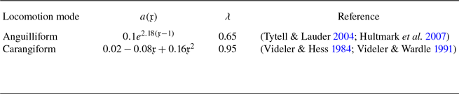
for two modes of locomotion and corresponding references can be found in table 1. In the context of swimming, the Strouhal number is defined as
$\lambda$
for two modes of locomotion and corresponding references can be found in table 1. In the context of swimming, the Strouhal number is defined as $St_0={fA}/U_0$
(Triantafyllou et al. Reference Triantafyllou, Triantafyllou and Gopalkrishnan1991), where
$St_0={fA}/U_0$
(Triantafyllou et al. Reference Triantafyllou, Triantafyllou and Gopalkrishnan1991), where $f$
is the undulation frequency,
$f$
is the undulation frequency, $A$
is the maximum lateral excursion of tail tip and
$A$
is the maximum lateral excursion of tail tip and $U_0$
is the nominal swimming speed.
$U_0$
is the nominal swimming speed.
Table 1. Amplitude envelope function $a(\mathfrak x)$
and wavelength
$a(\mathfrak x)$
and wavelength $\lambda$
for two modes of locomotion.
$\lambda$
for two modes of locomotion.
It should be noted that, according to (2.5), the length of the swimmers changes slightly during a cycle (less than 2 % for the travelling wave and less than 5 % for the standing wave). Nevertheless, the conservation of mass around the body is satisfied using a correction factor in every time step (Borazjani et al. Reference Borazjani, Ge, Le and Sotiropoulos2013). Consequently, this minor change of the swimmer’s length does not affect the physics of the problem. Thus, the wave kinematics can be considered a reliable approximation of actual swimming motion, as demonstrated in previous numerical simulations (Van Rees et al. Reference van Rees, Gazzola and Koumoutsakos2015; Li et al. Reference Li, Müller, van Leeuwen and Liu2016).
2.3. Computational details
The length, cruising speed (chosen as characteristic length and speed, respectively) and undulation frequency of lampreys are reported as $L=0.18 $
m,
$L=0.18 $
m, $U_0=0.22\ \textrm{m}\:\textrm{s}^{-1}$
and
$U_0=0.22\ \textrm{m}\:\textrm{s}^{-1}$
and $f= 3.1 $
Hz in the experimental observations (Tytell Reference Tytell2004; Tytell & Lauder Reference Tytell and Lauder2004). Physical properties of water at room temperature are also considered as
$f= 3.1 $
Hz in the experimental observations (Tytell Reference Tytell2004; Tytell & Lauder Reference Tytell and Lauder2004). Physical properties of water at room temperature are also considered as $\rho =998\ \textrm {kg} \, \textrm {m}^{-3}$
(density of water),
$\rho =998\ \textrm {kg} \, \textrm {m}^{-3}$
(density of water), $\nu =1.0 \times 10^{-6}$ $\textrm {m}^2 \:\textrm {s}^{-1}$
(kinematics viscosity of water). We used the experimental length and speed of the swimmers to non-dimensionalise the parameters, since the numerical swimming speed cannot be determined a priori (Daghooghi & Borazjani Reference Daghooghi and Borazjani2015, Reference Daghooghi and Borazjani2016; Li et al. Reference Li, Müller, van Leeuwen and Liu2016). Using the experimental values for frequency, characteristic length and speed (Tytell Reference Tytell2004), the initial Reynolds and Strouhal numbers for the lamprey are set as
$\textrm {m}^2 \:\textrm {s}^{-1}$
(kinematics viscosity of water). We used the experimental length and speed of the swimmers to non-dimensionalise the parameters, since the numerical swimming speed cannot be determined a priori (Daghooghi & Borazjani Reference Daghooghi and Borazjani2015, Reference Daghooghi and Borazjani2016; Li et al. Reference Li, Müller, van Leeuwen and Liu2016). Using the experimental values for frequency, characteristic length and speed (Tytell Reference Tytell2004), the initial Reynolds and Strouhal numbers for the lamprey are set as $Re_0=(\rho U_0 L)/\mu =40\,000$
and
$Re_0=(\rho U_0 L)/\mu =40\,000$
and $St_0=0.5$
. This value of Strouhal number falls within the typical range observed in nature for elongated fish such as eels and lampreys (Triantafyllou et al. Reference Triantafyllou, Triantafyllou and Gopalkrishnan1991). For ease of comparison, the mackerel is assumed to swim at a similar Reynolds number as the lamprey. At
$St_0=0.5$
. This value of Strouhal number falls within the typical range observed in nature for elongated fish such as eels and lampreys (Triantafyllou et al. Reference Triantafyllou, Triantafyllou and Gopalkrishnan1991). For ease of comparison, the mackerel is assumed to swim at a similar Reynolds number as the lamprey. At $Re_0=40\,000$
, the Strouhal number (frequency) is chosen to be
$Re_0=40\,000$
, the Strouhal number (frequency) is chosen to be $St_0=0.3$
based on the previous self-propelled simulations of a mackerel (Daghooghi & Borazjani Reference Daghooghi and Borazjani2015). Because
$St_0=0.3$
based on the previous self-propelled simulations of a mackerel (Daghooghi & Borazjani Reference Daghooghi and Borazjani2015). Because $Re_0$
and
$Re_0$
and $St_0$
are set based on experimental measurements and numerical simulations, we expect the calculated swimming speed
$St_0$
are set based on experimental measurements and numerical simulations, we expect the calculated swimming speed $U_s$
at a quasisteady state to closely match the experimental nominal speed
$U_s$
at a quasisteady state to closely match the experimental nominal speed $U_0$
. In other words, the actual Reynolds (
$U_0$
. In other words, the actual Reynolds ( $Re=\rho U_s L/\mu$
) and Strouhal (
$Re=\rho U_s L/\mu$
) and Strouhal ( $St={fA}/U_s$
) numbers should be approximately equal to their nominal values (
$St={fA}/U_s$
) numbers should be approximately equal to their nominal values ( $Re_0,St_0$
), respectively. If this expectation met, it will serve as a validation of our simulations.
$Re_0,St_0$
), respectively. If this expectation met, it will serve as a validation of our simulations.
The three self-propelled swimmers (two lampreys and a mackerel) swim in the horizontal plane with two degrees of freedom for their COM, i.e. the swimmers’ COM can move axially as well as laterally, the $x$
and
$x$
and $z$
directions, respectively. The computational domain for lampreys, shown in figure 2(b), is a cuboid with dimensions
$z$
directions, respectively. The computational domain for lampreys, shown in figure 2(b), is a cuboid with dimensions $2L \times L \times 20L$
, which is discretised with
$2L \times L \times 20L$
, which is discretised with $201 \times 121 \times 601$
(approximately
$201 \times 121 \times 601$
(approximately $14.6\times 10^6$
) grid nodes. A uniform high-resolution mesh with constant spacing
$14.6\times 10^6$
) grid nodes. A uniform high-resolution mesh with constant spacing $\Delta x= 0.008L$
in length,
$\Delta x= 0.008L$
in length, $\Delta y=0.002L$
in height and
$\Delta y=0.002L$
in height and $\Delta z=0.004L$
in width is used to discretise an inner cuboid (with dimensions
$\Delta z=0.004L$
in width is used to discretise an inner cuboid (with dimensions $0.4L \times 0.1L \times 1.5L$
enclosing the lamprey at all times) in order to resolve the near-field vortex structure. With this resolution, non-dimensional wall distance in the lateral direction would be small enough (
$0.4L \times 0.1L \times 1.5L$
enclosing the lamprey at all times) in order to resolve the near-field vortex structure. With this resolution, non-dimensional wall distance in the lateral direction would be small enough ( $y^+ \lt 10$
) to accurately model turbulent flow near the surface. Virtual lampreys are placed
$y^+ \lt 10$
) to accurately model turbulent flow near the surface. Virtual lampreys are placed $5L$
from the inlet plane in the axial direction and centred in the transverse and vertical directions. The non-dimensional time period of the tail-beat cycle is
$5L$
from the inlet plane in the axial direction and centred in the transverse and vertical directions. The non-dimensional time period of the tail-beat cycle is $T=2a_{max}/St_0$
for both the swimmers. Each tail-beat cycle is divided into 300 steps, which makes the non-dimensional time step equal to
$T=2a_{max}/St_0$
for both the swimmers. Each tail-beat cycle is divided into 300 steps, which makes the non-dimensional time step equal to $1.33 \times 10^{-3}$
.
$1.33 \times 10^{-3}$
.
For the mackerel, the computational domain has dimensions of $2L \times 2L \times 7L$
and is discretised with
$2L \times 2L \times 7L$
and is discretised with $201 \times 201 \times 501$
(approximately
$201 \times 201 \times 501$
(approximately $20.2\times 10^6$
) grid nodes. The larger domain size in the vertical (
$20.2\times 10^6$
) grid nodes. The larger domain size in the vertical ( $y$
) direction accounts for the greater dorsoventral size of the mackerel (
$y$
) direction accounts for the greater dorsoventral size of the mackerel ( $0.2L$
), compared with the lamprey’s dorsoventral size (
$0.2L$
), compared with the lamprey’s dorsoventral size ( $0.066L$
). The smaller domain in the streamwise (
$0.066L$
). The smaller domain in the streamwise ( $x$
) direction, compared with the lamprey’s domain, aligns with our previous work (Borazjani & Sotiropoulos Reference Borazjani and Sotiropoulos2010; Daghooghi & Borazjani Reference Daghooghi and Borazjani2015). Despite being shorter, it is still sufficiently large to prevent boundary effects from influencing the results. Similar to the lamprey’s computational domain, there is a uniform high-resolution mesh with constant spacing (with dimensions
$x$
) direction, compared with the lamprey’s domain, aligns with our previous work (Borazjani & Sotiropoulos Reference Borazjani and Sotiropoulos2010; Daghooghi & Borazjani Reference Daghooghi and Borazjani2015). Despite being shorter, it is still sufficiently large to prevent boundary effects from influencing the results. Similar to the lamprey’s computational domain, there is a uniform high-resolution mesh with constant spacing (with dimensions $0.22L \times 0.22L \times 1.04L$
) surrounding the mackerel at all times with
$0.22L \times 0.22L \times 1.04L$
) surrounding the mackerel at all times with $\Delta x= 0.004L$
in length,
$\Delta x= 0.004L$
in length, $\Delta y=0.002L$
in height and
$\Delta y=0.002L$
in height and $\Delta z=0.002L$
, in this case
$\Delta z=0.002L$
, in this case $y^+ \lt 5$
. The mackerel is placed at
$y^+ \lt 5$
. The mackerel is placed at $1.5L$
away from the inlet and the tail-beat of the mackerel is also divided into 300 time steps per cycle which in this case makes the non-dimensional time step equal to
$1.5L$
away from the inlet and the tail-beat of the mackerel is also divided into 300 time steps per cycle which in this case makes the non-dimensional time step equal to $2.22 \times 10^{-3}$
. The lamprey and mackerel geometries are discretised using 3384 and 29 859 triangular elements, respectively, to accurately capture the geometries. A homogeneous Neumann (far-field) boundary condition is used for the velocity at all outer boundaries.
$2.22 \times 10^{-3}$
. The lamprey and mackerel geometries are discretised using 3384 and 29 859 triangular elements, respectively, to accurately capture the geometries. A homogeneous Neumann (far-field) boundary condition is used for the velocity at all outer boundaries.
2.4. Flow and pressure visualisation
Vortical structures around swimmers are visualised by the isosurfaces of the $Q$
-criteria (Hunt et al. Reference Hunt, Wray and Moin1988). The
$Q$
-criteria (Hunt et al. Reference Hunt, Wray and Moin1988). The $Q$
-criterion is defined as
$Q$
-criterion is defined as
 \begin{align} Q=\frac {1}{2}\left ( \| \Psi \|^2 -\| \Phi \|^2 \right ) , \end{align}
where $\Psi$
and
$\Psi$
and $\Phi$
denote the asymmetric and symmetric parts of the dimensionless velocity gradient, respectively, and
$\Phi$
denote the asymmetric and symmetric parts of the dimensionless velocity gradient, respectively, and $\| \bullet \|$
is the Euclidean matrix norm. Positive
$\| \bullet \|$
is the Euclidean matrix norm. Positive $Q$
isosurfaces are regions where the rotation rate dominates the strain rate.
$Q$
isosurfaces are regions where the rotation rate dominates the strain rate.
The vorticity field is non-dimensionalised by $U_0/L$
in all of the flow visualisations reported in this article, and the pressure field is non-dimensionalised by the dynamic pressure (
$U_0/L$
in all of the flow visualisations reported in this article, and the pressure field is non-dimensionalised by the dynamic pressure ( $\rho U_0^2$
). The pressure is calculated relative to one of the corner points of the computational domain, far away from the swimmer, since pressure plus any constant satisfies the fluid governing equations. Calculating the pressure relative to another point on the boundary changes the pressure by a small amount.
$\rho U_0^2$
). The pressure is calculated relative to one of the corner points of the computational domain, far away from the swimmer, since pressure plus any constant satisfies the fluid governing equations. Calculating the pressure relative to another point on the boundary changes the pressure by a small amount.
2.5. Calculation of acceleration, AoA, force and power
Considering equation (2.5) for body undulation in the $z$
-direction, a swimmer with a non-dimensional cruising speed
$z$
-direction, a swimmer with a non-dimensional cruising speed $U$
in the
$U$
in the $x$
-direction generates a non-dimensional lateral velocity
$x$
-direction generates a non-dimensional lateral velocity $w$
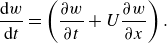
of a fluid particle adjacent to the body. In an ideal flow following the motion of the body (figure 1
a), this velocity is given by the material derivative (Lighthill Reference Lighthill1960),
$w$
of a fluid particle adjacent to the body. In an ideal flow following the motion of the body (figure 1
a), this velocity is given by the material derivative (Lighthill Reference Lighthill1960),
 \begin{align} w= \frac {\textrm {d} h}{\textrm {d} t}=\frac {\partial h}{\partial t} + U \frac {\partial h}{\partial x} . \end{align}
The instantaneous non-dimensional acceleration of a fluid particle in the $z$
-direction is obtained by taking the material derivative of the velocity
$z$
-direction is obtained by taking the material derivative of the velocity $w$
:
$w$
:
 \begin{align} \frac {\textrm {d} w}{\textrm {d} t}= \left ( \frac {\partial w}{\partial t} + U \frac {\partial w}{\partial x} \right ) . \end{align}
The other two components of convective acceleration vector (in $x$
- and
$x$
- and $y$
-directions) are considered negligible during steady swimming. The non-dimensional normal acceleration of a fluid particle is calculated by taking into account the outward normal direction of the surface
$y$
-directions) are considered negligible during steady swimming. The non-dimensional normal acceleration of a fluid particle is calculated by taking into account the outward normal direction of the surface $\mathbf{n}$
(with
$\mathbf{n}$
(with $n_z$
component in the
$n_z$
component in the $z$
-direction):
$z$
-direction):
 \begin{align} a_n=\frac {\textrm {d} w}{\textrm {d} t} n_z . \end{align}
The above normal acceleration represents the pressure difference generated by the added mass (reactive force) mechanism, see Appendix A.
The lift-based force is estimated using the AoA, because the lift force is typically proportional to the AoA until the stall angle. The AoA ( $\alpha$
) is defined as the angle between the body’s reference line and the relative velocity. The angle
$\alpha$
) is defined as the angle between the body’s reference line and the relative velocity. The angle $\theta$
made by the reference line of the body with the streamwise
$\theta$
made by the reference line of the body with the streamwise $x$
direction at any time instant can be calculated from the slope (
$x$
direction at any time instant can be calculated from the slope ( $\theta = \tan ^{-1}(\partial h / \partial x$
). As shown in figure 1(b), the angle between the relative velocity and the streamwise
$\theta = \tan ^{-1}(\partial h / \partial x$
). As shown in figure 1(b), the angle between the relative velocity and the streamwise $x$
direction is given by
$x$
direction is given by $\gamma = \tan ^{-1}(- ({1}/{U})\partial h / \partial t)$
. From figure 1(b), the AoA is
$\gamma = \tan ^{-1}(- ({1}/{U})\partial h / \partial t)$
. From figure 1(b), the AoA is $\alpha = \gamma - \theta$
. To account for the opposite pressure distributions on lateral sides (figure 1
b), the AoA is modified using the outward normal direction (
$\alpha = \gamma - \theta$
. To account for the opposite pressure distributions on lateral sides (figure 1
b), the AoA is modified using the outward normal direction ( $n_z/|n_z|$
):
$n_z/|n_z|$
):
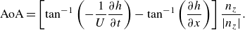 \begin{align} \text {AoA} = \left [\tan ^{-1} \left (-\frac {1}{U}\frac {\partial h}{\partial t} \right ) - \tan ^{-1} \left (\frac {\partial h}{\partial x} \right ) \right ] \frac {n_z}{|n_z|} . \end{align}
The term ‘AoA’ is used hereafter as a measure of pressure generated by the lift-based mechanism as per (2.10).
The instantaneous non-dimensional hydrodynamic force component in each direction, (e.g. $F_1(t)$
in the
$F_1(t)$
in the $x$
direction) is computed by integrating the pressure and viscous forces acting on the body as follows (where repeated indices imply summation):
$x$
direction) is computed by integrating the pressure and viscous forces acting on the body as follows (where repeated indices imply summation):
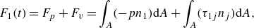 \begin{align} F_1(t)=F_p+F_v=\int _A (-pn_1) \text {d}A+\int _A (\tau _{1j}n_j) \text {d}A , \end{align}
where $p$
is the non-dimensional pressure,
$p$
is the non-dimensional pressure, $\tau$
is the non-dimensional viscous stress tensor, and
$\tau$
is the non-dimensional viscous stress tensor, and $n_j$
is the
$n_j$
is the $j$
th component of the unit normal vector on the body surface. Depending on whether non-dimensional pressure force
$j$
th component of the unit normal vector on the body surface. Depending on whether non-dimensional pressure force $F_p$
or viscous force
$F_p$
or viscous force $F_v$
is negative or positive (considering swimming along the positive
$F_v$
is negative or positive (considering swimming along the positive $x$
direction), they may contribute to either drag or thrust. Therefore, following our numerical set-up in figure 2 and (2.11), thrust force,
$x$
direction), they may contribute to either drag or thrust. Therefore, following our numerical set-up in figure 2 and (2.11), thrust force, $C_T$
is calculated as follows (Borazjani & Sotiropoulos Reference Borazjani and Sotiropoulos2008):
$C_T$
is calculated as follows (Borazjani & Sotiropoulos Reference Borazjani and Sotiropoulos2008):
 \begin{align} C_T(t)=\frac {1}{2}\left [\int _A -p n_1 \, \textrm {d}A+\left |\int _A -p n_1 \, \textrm {d}A\right |\right ] +\frac {1}{2}\left [\int _A \tau _{1j}n_j \, \textrm {d}A+\left |\int _A \tau _{1j}n_j \, \textrm {d}A\right |\right ] . \end{align}
Note that $F_v$
is typically negative (acts as a drag) and does not contribute to thrust. The non-dimensional power consumption
$F_v$
is typically negative (acts as a drag) and does not contribute to thrust. The non-dimensional power consumption $E$
due to lateral undulations (
$E$
due to lateral undulations ( $z$
-direction) of the fish body is calculated by multiplying lateral force to the lateral velocity as
$z$
-direction) of the fish body is calculated by multiplying lateral force to the lateral velocity as
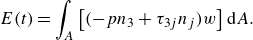 \begin{align} E(t)=\int _A \left [(-pn_3+\tau _{3j}n_j)w\right ] \text {d}A . \end{align}
Finally, following Lighthill (Reference Lighthill1960) the swimming efficiency (referred to as the Froude efficiency) is defined as
 \begin{align} \eta _F = C_T U/ (C_T U + E) , \end{align}
where $U$
,
$U$
, $C_T$
and
$C_T$
and $E$
are the cycle-averaged non-dimensional swimming speed, thrust force and power, respectively. Note that this efficiency should be computed during quasisteady state to be meaningful (Borazjani & Sotiropoulos Reference Borazjani and Sotiropoulos2008).
$E$
are the cycle-averaged non-dimensional swimming speed, thrust force and power, respectively. Note that this efficiency should be computed during quasisteady state to be meaningful (Borazjani & Sotiropoulos Reference Borazjani and Sotiropoulos2008).
3. Results
Two virtual lampreys of equal size and identical geometry – one undulating with the travelling wave and the other with the standing wave (2.5) – along with a mackerel are released in an initially stagnant fluid under the conditions stated in § 2.3. As they start undulating, their instantaneous swimming speeds increase over time (shown in figure 3 a) until they reach a quasisteady state, when drag and thrust forces become equal and the net force over one cycle averages to zero, see figures 3 and 4. The instantaneous swimming speed fluctuates slightly within each undulation cycle as thrust and drag forces vary depending on the kinematics of undulations. This phenomenon has been reported in previous simulations (Borazjani & Sotiropoulos Reference Borazjani and Sotiropoulos2009) and experimental observations (Müller et al. Reference Müller, Smit, Stamhuis and Videler2001). The amplitude of these fluctuations are much smaller for the anguilliform swimmer with the travelling wave than the one with the standing wave (figure 3 a). The amplitude of fluctuations for the carangiform swimmer with the travelling wave kinematics is higher than both anguilliform swimmers.
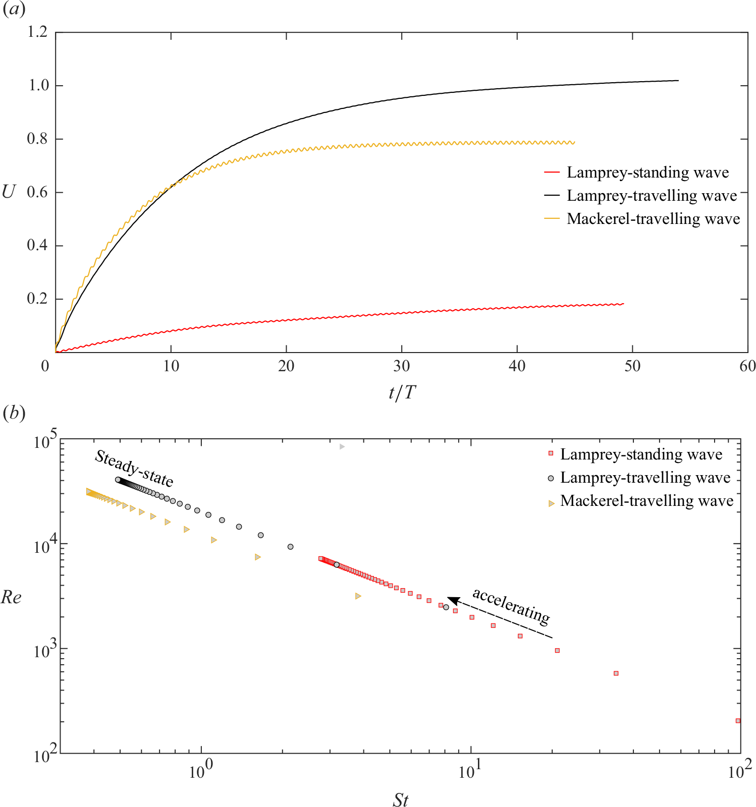
Figure 3. (a) The time history of non-dimensional swimming speed $U=U_s/U_0$
is shown for three virtual simmers starting from rest to steady-state. (b) Reynolds number and Strouhal number at each tailbeat cycle are calculated based on the cycle-averaged swimming speed.
$U=U_s/U_0$
is shown for three virtual simmers starting from rest to steady-state. (b) Reynolds number and Strouhal number at each tailbeat cycle are calculated based on the cycle-averaged swimming speed.
For each cycle, the average swimming speed can be calculated according to $U_{cyc} = (1/T) \int U_s \text {d}t$
and at the quasisteady this value remains constant. The cycle-averaged swimming speeds during the quasisteady state for the model lamprey and the model mackerel with the travelling wave are
$U_{cyc} = (1/T) \int U_s \text {d}t$
and at the quasisteady this value remains constant. The cycle-averaged swimming speeds during the quasisteady state for the model lamprey and the model mackerel with the travelling wave are $U_{cyc}/U_0 =1.02$
and
$U_{cyc}/U_0 =1.02$
and $U_{cyc}/U_0 =0.787$
, respectively. In contrast, the lamprey with the standing wave swims significantly slower, with an average speed of
$U_{cyc}/U_0 =0.787$
, respectively. In contrast, the lamprey with the standing wave swims significantly slower, with an average speed of $U_{cyc}/U_0 = 0.18$
. The significant difference in swimming speeds between travelling and standing wave kinematics is in agreement with our previous study on folding structures (Daghooghi & Borazjani Reference Daghooghi and Borazjani2016). The lower swimming speed of the mackerel compared with the lamprey is likely due to its lower prescribed tail beat frequency
$U_{cyc}/U_0 = 0.18$
. The significant difference in swimming speeds between travelling and standing wave kinematics is in agreement with our previous study on folding structures (Daghooghi & Borazjani Reference Daghooghi and Borazjani2016). The lower swimming speed of the mackerel compared with the lamprey is likely due to its lower prescribed tail beat frequency $St_0$
in a similar fluid environment, see § 2.3. Furthermore, the computed swimming speed
$St_0$
in a similar fluid environment, see § 2.3. Furthermore, the computed swimming speed $U_{cyc}/U_0$
of the anguilliform swimmer using the travelling wave is very close to unity, indicating the computed swimming speed
$U_{cyc}/U_0$
of the anguilliform swimmer using the travelling wave is very close to unity, indicating the computed swimming speed $U_{cyc}$
aligns closely to the nominal experimental swimming speed
$U_{cyc}$
aligns closely to the nominal experimental swimming speed $U_0$
reported in observations (Tytell Reference Tytell2004). The recovery of the nominal swimming speed (
$U_0$
reported in observations (Tytell Reference Tytell2004). The recovery of the nominal swimming speed ( $U=U_s/U_0 \approx 1$
) in the simulations with prescribed eel kinematics (Tytell Reference Tytell2004) serves as an important validation of our self-propelled simulations.
$U=U_s/U_0 \approx 1$
) in the simulations with prescribed eel kinematics (Tytell Reference Tytell2004) serves as an important validation of our self-propelled simulations.
Based on the cycle-averaged swimming speeds, the Reynolds and Strouhal numbers are calculated and plotted in figure 3(b). During the acceleration phase (approximately the first 15 cycles), swimming speed and consequently the Reynolds number increase rapidly. Since the Strouhal number is inversely proportional to the swimming speed, it decreases sharply during this phase. As shown in these figures, our simulation covers different regimes of flow, transitioning from a laminar flow in the early cycles to a turbulent flow at the quasisteady state. In the quasisteady state, the Reynolds and Strouhal numbers are calculated and summarised in table 2. It can be observed that, within the same range of Reynolds numbers, the Strouhal number for the mackerel is lower than that for the lamprey. This is consistent with the finding of Borazjani & Sotiropoulos (Reference Borazjani and Sotiropoulos2010) who compared anguilliform and carangiform swimmers at similar Reynolds numbers.
Table 2. Hydrodynamic parameters of three swimmers at the quasisteady state: non-dimensional cycle-averaged swimming speed $U_{cyc}/U_0$
; Reynolds number
$U_{cyc}/U_0$
; Reynolds number $Re$
; Strouhal number
$Re$
; Strouhal number $St$
; non-dimensional cycle-averaged thrust force
$St$
; non-dimensional cycle-averaged thrust force $C_T$
; non-dimensional cycle-averaged power consumption
$C_T$
; non-dimensional cycle-averaged power consumption $E$
; Froude efficiency
$E$
; Froude efficiency $\eta _F$
.
$\eta _F$
.
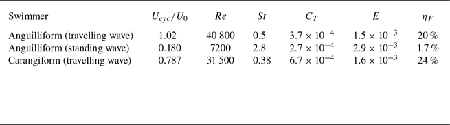
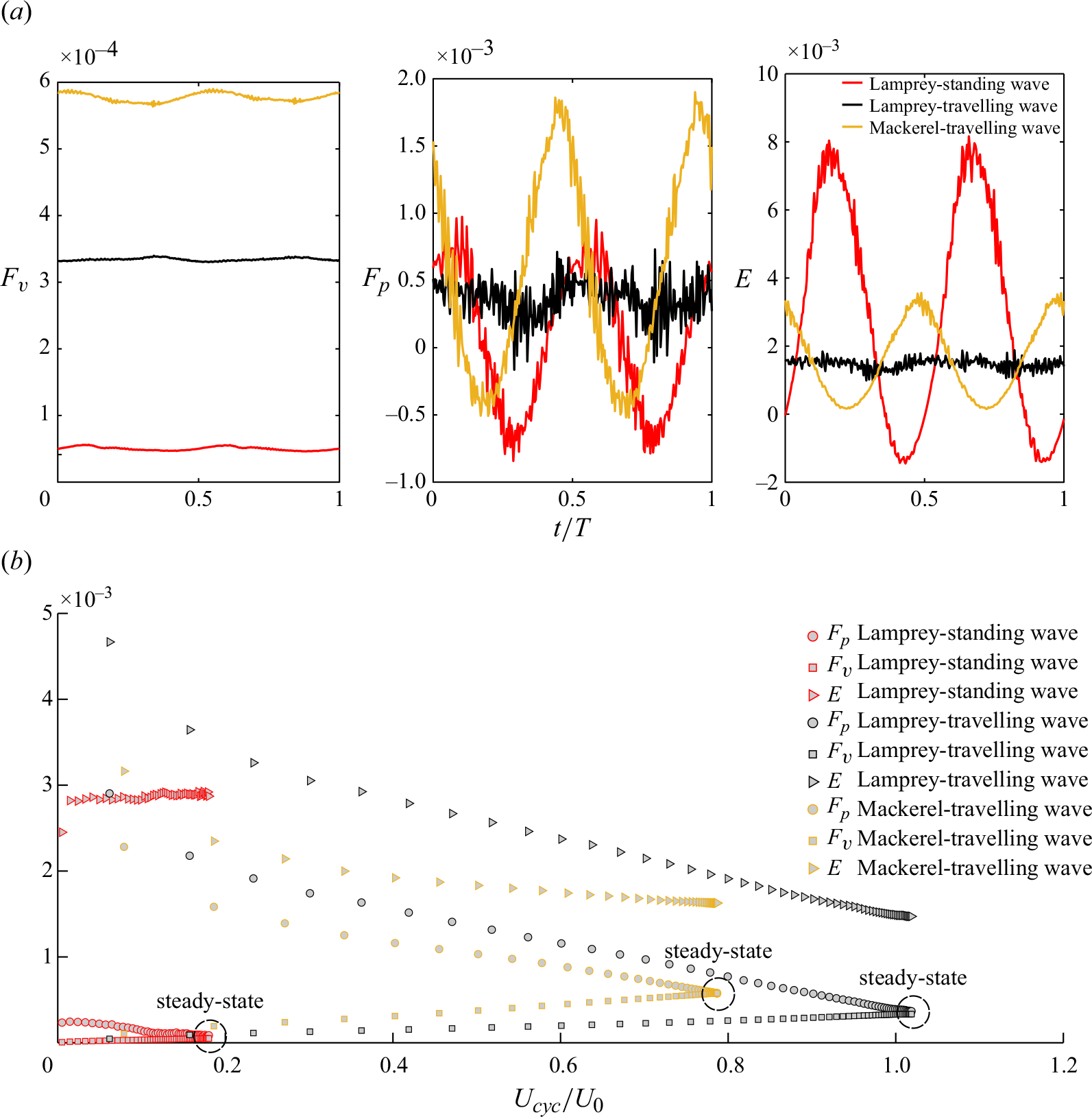
Figure 4. (a) Non-dimensional instantaneous viscous force ( $F_v$
), non-dimensional instantaneous pressure force (
$F_v$
), non-dimensional instantaneous pressure force ( $F_p$
) and non-dimensional instantaneous power are shown during one cycle at quasisteady state. (b) Non-dimensional cycle-averaged pressure force
$F_p$
) and non-dimensional instantaneous power are shown during one cycle at quasisteady state. (b) Non-dimensional cycle-averaged pressure force $F_p$
, viscous force
$F_p$
, viscous force $F_v$
and lateral power consumption
$F_v$
and lateral power consumption $E$
are shown as a function of non-dimensional cycle-averaged swimming velocity
$E$
are shown as a function of non-dimensional cycle-averaged swimming velocity $U_{cyc}/U_0$
.
$U_{cyc}/U_0$
.
The time history of non-dimensional instantaneous pressure force $F_p$
, viscous force
$F_p$
, viscous force $F_v$
and power
$F_v$
and power $E$
are shown in figure 4(a), demonstrating two peaks per cycle corresponding to a back-and-forth tail beat. The viscous force always acts in the drag direction for all swimmers and shows the least variation over time because shear stress is proportional to the velocity gradient, and the swimming velocity does not vary significantly during a cycle. The pressure force for the mackerel exhibits a much higher amplitude compared with that of the lamprey using the travelling wave. The pressure force generated by the lamprey using the travelling wave has the smallest amplitude of oscillations but remains consistently positive, i.e. thrust-generating. In contrast, the mackerel generates much stronger pressure forces at certain instances, but these forces can also become negative, i.e. drag-inducing. For the lamprey using the standing wave, the pressure force oscillates almost symmetrically between positive and negative values, resulting in a near-zero cycle-averaged value. The highest amplitude and average power consumption are observed in the lamprey using the standing wave, followed by the mackerel, and then the lamprey with travelling wave kinematics. It can be observed that the
$E$
are shown in figure 4(a), demonstrating two peaks per cycle corresponding to a back-and-forth tail beat. The viscous force always acts in the drag direction for all swimmers and shows the least variation over time because shear stress is proportional to the velocity gradient, and the swimming velocity does not vary significantly during a cycle. The pressure force for the mackerel exhibits a much higher amplitude compared with that of the lamprey using the travelling wave. The pressure force generated by the lamprey using the travelling wave has the smallest amplitude of oscillations but remains consistently positive, i.e. thrust-generating. In contrast, the mackerel generates much stronger pressure forces at certain instances, but these forces can also become negative, i.e. drag-inducing. For the lamprey using the standing wave, the pressure force oscillates almost symmetrically between positive and negative values, resulting in a near-zero cycle-averaged value. The highest amplitude and average power consumption are observed in the lamprey using the standing wave, followed by the mackerel, and then the lamprey with travelling wave kinematics. It can be observed that the $E$
becomes negative at some intervals for the lamprey with standing waves, but not for the others, which indicates that it extracts energy from the fluid. The negative power intervals, however, have smaller peaks and shorter duration compared with positive ones, i.e. net power consumption rather than extraction. The negative power occurs when the body motion is in the same direction as the pressure gradient (force) in the lateral direction, which was previously reported for a mackerel in an inviscid flow (Borazjani & Sotiropoulos Reference Borazjani and Sotiropoulos2010). The mackerel here, similar to mackerels at lower
$E$
becomes negative at some intervals for the lamprey with standing waves, but not for the others, which indicates that it extracts energy from the fluid. The negative power intervals, however, have smaller peaks and shorter duration compared with positive ones, i.e. net power consumption rather than extraction. The negative power occurs when the body motion is in the same direction as the pressure gradient (force) in the lateral direction, which was previously reported for a mackerel in an inviscid flow (Borazjani & Sotiropoulos Reference Borazjani and Sotiropoulos2010). The mackerel here, similar to mackerels at lower $Re$
of approximately 4000 and 300 (Borazjani & Sotiropoulos Reference Borazjani and Sotiropoulos2010), does not show negative peaks.
$Re$
of approximately 4000 and 300 (Borazjani & Sotiropoulos Reference Borazjani and Sotiropoulos2010), does not show negative peaks.
The cycle-averaged pressure force $F_p$
(thrust type), viscous force
$F_p$
(thrust type), viscous force $F_v$
(drag type due to fluid viscosity) and power consumption
$F_v$
(drag type due to fluid viscosity) and power consumption $E$
are plotted as functions of cycle-averaged swimming velocity in figure 4(b). For both types of kinematics and both swimmers, pressure force decreases while viscous force increases with the swimming speed. Ultimately, the viscous drag and pressure thrust forces become equal, resulting in net zero force after approximately 50 undulations. At this point, the swimmers reach quasisteady swimming. The increase in viscous force
$E$
are plotted as functions of cycle-averaged swimming velocity in figure 4(b). For both types of kinematics and both swimmers, pressure force decreases while viscous force increases with the swimming speed. Ultimately, the viscous drag and pressure thrust forces become equal, resulting in net zero force after approximately 50 undulations. At this point, the swimmers reach quasisteady swimming. The increase in viscous force $F_v$
with swimming speed is expected because the velocity gradient (and consequently wall shear stress) between the body and the fluid increases with speed. However, the reduction in pressure force as swimming speed increases is less intuitive and requires further investigation, which will be addressed in § 3.2.
$F_v$
with swimming speed is expected because the velocity gradient (and consequently wall shear stress) between the body and the fluid increases with speed. However, the reduction in pressure force as swimming speed increases is less intuitive and requires further investigation, which will be addressed in § 3.2.
A key observation from the plots shown in figure 4 is that the pressure force $F_p$
generated by the standing wave is one order of magnitude lower than that generated by the travelling wave (in both lamprey and mackerel) at a given speed
$F_p$
generated by the standing wave is one order of magnitude lower than that generated by the travelling wave (in both lamprey and mackerel) at a given speed $U$
from the very beginning. In contrast, the viscous force
$U$
from the very beginning. In contrast, the viscous force $F_v$
is initially comparable between both kinematics. As a result,
$F_v$
is initially comparable between both kinematics. As a result, $F_p$
of the standing wave reaches
$F_p$
of the standing wave reaches $F_v$
at a much lower swimming speed
$F_v$
at a much lower swimming speed $U$
compared with the travelling wave. The primary reason for this low thrust generation, and consequently lower forward acceleration and swimming speed, stems from the unreasonable nature of the standing wave kinematics for propulsion. As will be discussed in detail in § 3.2, the generated force from the pressure difference at some regions at the posterior part of the body is not aligned with the forward swimming direction. This undesirable pressure difference is converted into a drag (see figures 8
b and 8
d). In comparison, pressure difference at the posterior part of the lamprey employing travelling wave kinematics (figures 8
a and 8
c) generates a pressure force aligned with the swimming direction, i.e. the thrust-type pressure force
$U$
compared with the travelling wave. The primary reason for this low thrust generation, and consequently lower forward acceleration and swimming speed, stems from the unreasonable nature of the standing wave kinematics for propulsion. As will be discussed in detail in § 3.2, the generated force from the pressure difference at some regions at the posterior part of the body is not aligned with the forward swimming direction. This undesirable pressure difference is converted into a drag (see figures 8
b and 8
d). In comparison, pressure difference at the posterior part of the lamprey employing travelling wave kinematics (figures 8
a and 8
c) generates a pressure force aligned with the swimming direction, i.e. the thrust-type pressure force $F_p$
is significantly stronger.
$F_p$
is significantly stronger.
When a swimmer propels through water using lateral movements with a lateral velocity of $\partial h/ \partial t$
, it changes the momentum of the adjacent fluid, which requires energy consumption. The rate of energy consumption, represented as power
$\partial h/ \partial t$
, it changes the momentum of the adjacent fluid, which requires energy consumption. The rate of energy consumption, represented as power $E$
is given by (2.13), and its cycle-averaged values are shown in figure 4(b). For travelling wave kinematics, the power consumption decreases as the lamprey and mackerel gain speed. In contrast, for the standing wave kinematics, the rate of work does not change significantly and stays almost constant. When comparing the swimmers at their quasisteady states, the lamprey and mackerel employing travelling wave kinematics have consumed less energy to reach much higher speed than the swimmer using standing wave kinematics. This comparison highlights the considerable advantage of travelling wave kinematics in terms of swimming efficiency.
$E$
is given by (2.13), and its cycle-averaged values are shown in figure 4(b). For travelling wave kinematics, the power consumption decreases as the lamprey and mackerel gain speed. In contrast, for the standing wave kinematics, the rate of work does not change significantly and stays almost constant. When comparing the swimmers at their quasisteady states, the lamprey and mackerel employing travelling wave kinematics have consumed less energy to reach much higher speed than the swimmer using standing wave kinematics. This comparison highlights the considerable advantage of travelling wave kinematics in terms of swimming efficiency.
The hydrodynamic performance of three swimmers at quasisteady state is summarised in table 2, demonstrating superior performance of swimmers using travelling wave compared with the one using standing wave kinematics. The lamprey with the travelling wave generates an average thrust force $C_T= 3.7\times 10^{-4}$
(equal to dimensional value of
$C_T= 3.7\times 10^{-4}$
(equal to dimensional value of $0.58\ {\textrm{mN}}$
) and consuming energy at a rate equal to
$0.58\ {\textrm{mN}}$
) and consuming energy at a rate equal to $E = 1.5 \times 10^{-3}$
(equal to dimensional value of
$E = 1.5 \times 10^{-3}$
(equal to dimensional value of $0.52\ {\textrm{mW}}$
) in every cycle to maintain steady swimming speed. On the other hand, the mackerel with the travelling wave generates an average thrust force
$0.52\ {\textrm{mW}}$
) in every cycle to maintain steady swimming speed. On the other hand, the mackerel with the travelling wave generates an average thrust force $T= 6.8\times 10^{-4}$
(equal to dimensional value of
$T= 6.8\times 10^{-4}$
(equal to dimensional value of $1.1\ {\textrm{mN}}$
) and consuming energy at a rate equal to
$1.1\ {\textrm{mN}}$
) and consuming energy at a rate equal to $E = 1.6 \times 10^{-3}$
(equal to dimensional value of
$E = 1.6 \times 10^{-3}$
(equal to dimensional value of $0.55\ {\textrm{mW}}$
). This results in a Froude efficiency of
$0.55\ {\textrm{mW}}$
). This results in a Froude efficiency of $\eta _F =20\,\%$
for the lamprey and
$\eta _F =20\,\%$
for the lamprey and $\eta _F =24\,\%$
for the mackerel. In comparison, the average thrust force and power consumption for the standing wave lamprey are
$\eta _F =24\,\%$
for the mackerel. In comparison, the average thrust force and power consumption for the standing wave lamprey are $C_T= 2.7 \times 10^{-4}$
(0.43
$C_T= 2.7 \times 10^{-4}$
(0.43 ${\textrm{mN}}$
) and
${\textrm{mN}}$
) and $E = 2.9 \times 10^{-3}$
(
$E = 2.9 \times 10^{-3}$
( $0.99\ {\textrm{mW}}$
), resulting in a very low Froude efficiency
$0.99\ {\textrm{mW}}$
), resulting in a very low Froude efficiency $\eta _F =1.7\,\%$
during quasisteady swimming.
$\eta _F =1.7\,\%$
during quasisteady swimming.
3.1. Flow field and vorticity scaling
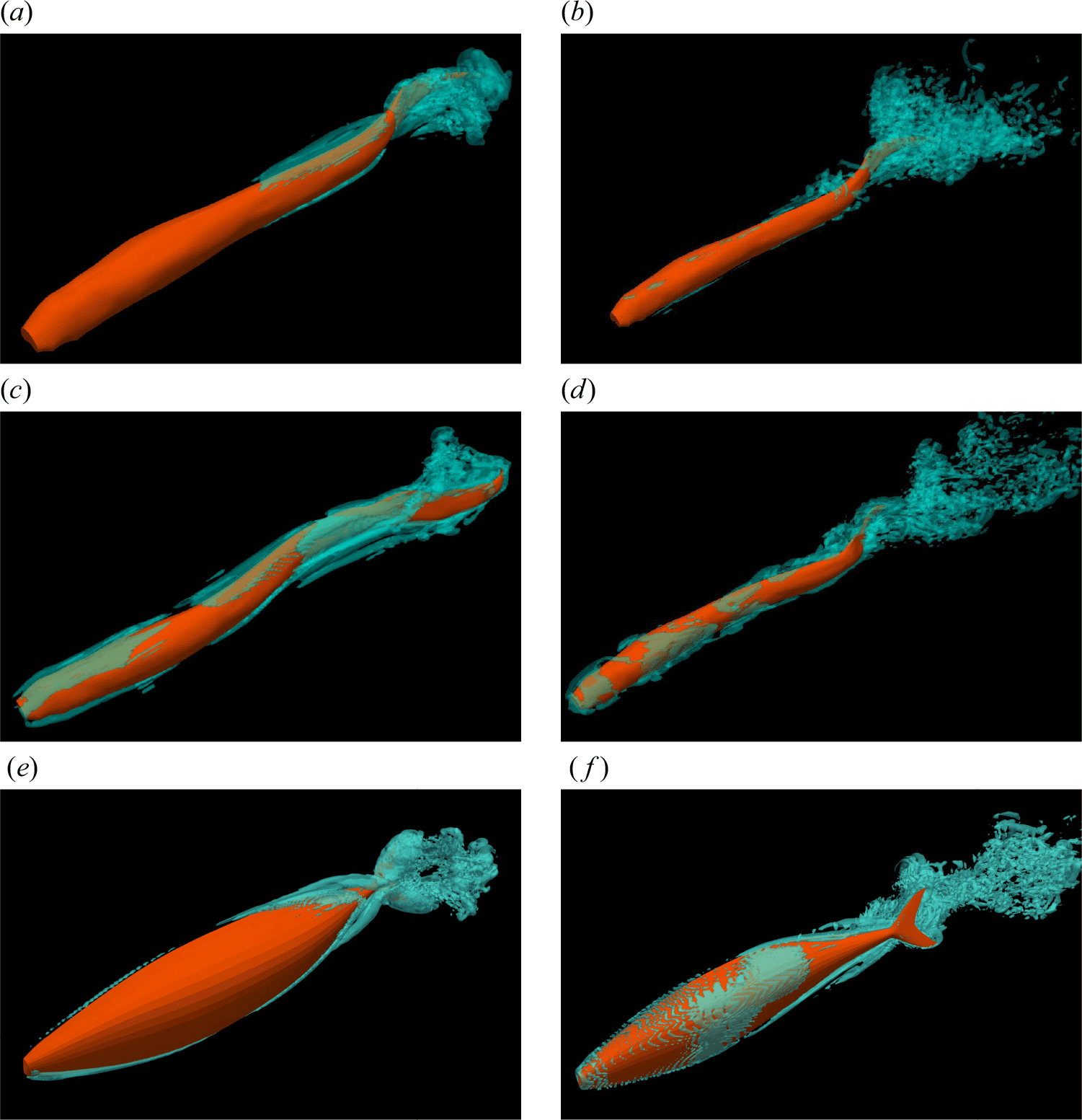
Figure 5. The 3-D wake structure visualised by the isosurfaces of $Q$
-criterion is shown for lamprey with standing (a,b) and travelling wave (c,d) and the mackerel with travelling wave (e,f). Panels (a,c,e) are from the first cycle, whereas panels (b,d,f) are from the quasisteady state.
$Q$
-criterion is shown for lamprey with standing (a,b) and travelling wave (c,d) and the mackerel with travelling wave (e,f). Panels (a,c,e) are from the first cycle, whereas panels (b,d,f) are from the quasisteady state.
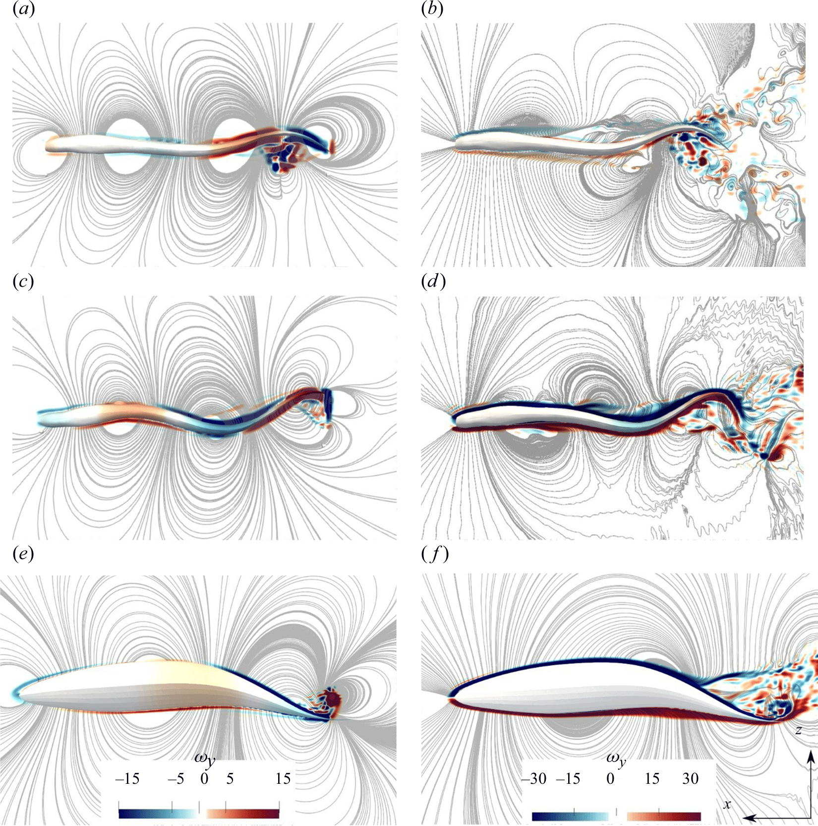
Figure 6. The non-dimensional vorticity contours on the horizontal midplane and on the body of the swimmer along with streamlines is shown for lamprey with standing (a,b) and travelling wave (c,d) and the mackerel with travelling wave (e,f). Panels (a,c,e) are from the first cycle, whereas panels (b,d,f) are from the quasisteady state. Fluid vorticity near the body follows the body rotation only at early cycles (a,c,e), but not at quasisteady (b,d,f). Note that the vorticity range in panels (a,c,e) is different than in panels (b,d,f), and the body vorticity is much smaller than the flow vorticity during quasisteady swimming (b,d,f).
The 3-D flow fields are visualised using isosurfaces of the $Q$
-criterion in figure 5 comparing standing (figure 5
a,b) and travelling wave kinematics (figure 5
c,d) for lampreys, as well as travelling wave kinematics (figure 5
e,f) for the mackerel. Figure 5(a,c,e) show the three swimmers during the first cycle of body undulation (lower
$Q$
-criterion in figure 5 comparing standing (figure 5
a,b) and travelling wave kinematics (figure 5
c,d) for lampreys, as well as travelling wave kinematics (figure 5
e,f) for the mackerel. Figure 5(a,c,e) show the three swimmers during the first cycle of body undulation (lower $Re$
) and figure 5(b,d,f) at quasisteady state (higher
$Re$
) and figure 5(b,d,f) at quasisteady state (higher $Re$
). During the first cycle of body undulation (low
$Re$
). During the first cycle of body undulation (low $Re$
and high
$Re$
and high $St$
), the wake behind the swimmers exhibits high lateral spreading indicating a double row of vortices due to high
$St$
), the wake behind the swimmers exhibits high lateral spreading indicating a double row of vortices due to high $St$
and well-organised structures due to low
$St$
and well-organised structures due to low $Re$
(figure 5
a,c,e). As swimmers reach the quasisteady state, the large coherent structures break down into smaller vortical structures due to the high Reynolds number
$Re$
(figure 5
a,c,e). As swimmers reach the quasisteady state, the large coherent structures break down into smaller vortical structures due to the high Reynolds number $Re$
of the flow. However, the type of wake (double row versus single row) varies between the swimmers (figure 5
b,d,f). For the standing wave swimmer, the high lateral spreading persists during quasisteady swimming due to its high
$Re$
of the flow. However, the type of wake (double row versus single row) varies between the swimmers (figure 5
b,d,f). For the standing wave swimmer, the high lateral spreading persists during quasisteady swimming due to its high $St$
(figure 5
b). For the travelling wave swimmers, however, the lateral spreading of the wake decreases (figure 5
d,f). The lamprey with travelling wave maintains a double row structure (figure 5
d), whereas the mackerel displays a single row structure (figure 5
f). This is because of the higher Strouhal number of lamprey (
$St$
(figure 5
b). For the travelling wave swimmers, however, the lateral spreading of the wake decreases (figure 5
d,f). The lamprey with travelling wave maintains a double row structure (figure 5
d), whereas the mackerel displays a single row structure (figure 5
f). This is because of the higher Strouhal number of lamprey ( $St$
= 0.5) at quasisteady state compared with the mackerel (
$St$
= 0.5) at quasisteady state compared with the mackerel ( $St$
= 0.38) as observed in table 2. The dependence of the wake structure and its lateral spreading on the Strouhal number is consistent with previous observations from both experimental (Müller et al. Reference Müller, Smit, Stamhuis and Videler2001; Tytell & Lauder Reference Tytell and Lauder2004; Hultmark et al. Reference Hultmark, Leftwich and Smits2007) and numerical (Borazjani & Sotiropoulos Reference Borazjani and Sotiropoulos2008, Reference Borazjani and Sotiropoulos2009) studies. Furthermore, the wake pattern aligns with the computed efficiency of the swimmer as the efficiency decreases with the increase in lateral spreading or, equivalently, with a higher Strouhal number
$St$
= 0.38) as observed in table 2. The dependence of the wake structure and its lateral spreading on the Strouhal number is consistent with previous observations from both experimental (Müller et al. Reference Müller, Smit, Stamhuis and Videler2001; Tytell & Lauder Reference Tytell and Lauder2004; Hultmark et al. Reference Hultmark, Leftwich and Smits2007) and numerical (Borazjani & Sotiropoulos Reference Borazjani and Sotiropoulos2008, Reference Borazjani and Sotiropoulos2009) studies. Furthermore, the wake pattern aligns with the computed efficiency of the swimmer as the efficiency decreases with the increase in lateral spreading or, equivalently, with a higher Strouhal number $St$
. As discussed by Borazjani & Sotiropoulos (Reference Borazjani and Sotiropoulos2010), higher lateral spreading generally indicates higher energy wasted in the lateral direction (related to
$St$
. As discussed by Borazjani & Sotiropoulos (Reference Borazjani and Sotiropoulos2010), higher lateral spreading generally indicates higher energy wasted in the lateral direction (related to $E$
defined in (2.13) rather than contributing to an increase in streamwise momentum (related to
$E$
defined in (2.13) rather than contributing to an increase in streamwise momentum (related to $C_T$
defined in (2.12)). This energy dissipation in lateral motion ultimately leads to a reduction in swimming efficiency (2.14).
$C_T$
defined in (2.12)). This energy dissipation in lateral motion ultimately leads to a reduction in swimming efficiency (2.14).
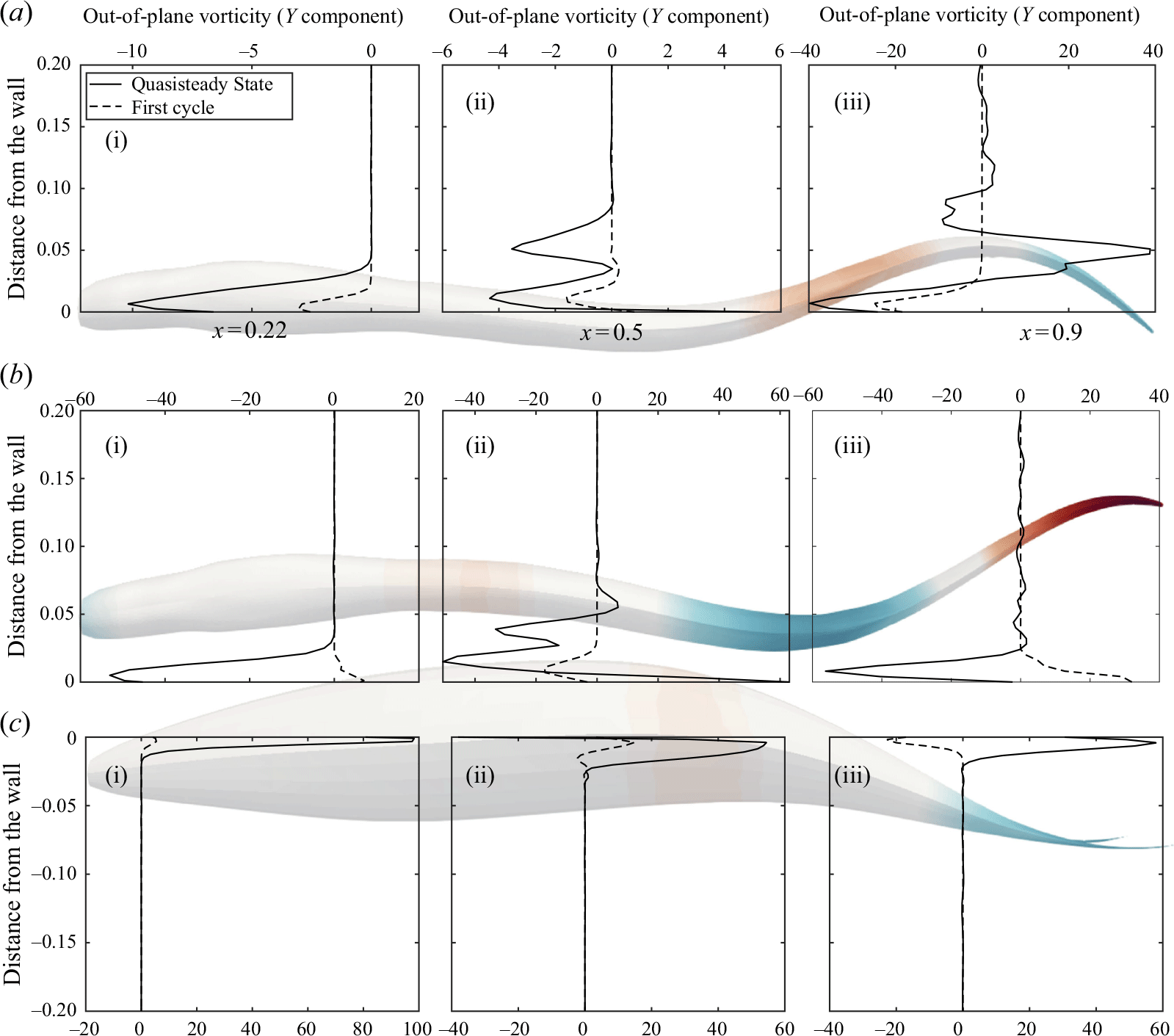
Figure 7. The non-dimensional vorticity at early cycles (dashed) and quasisteady state (solid lines) is plotted along the lateral $z$
direction at streamwise locations
$z$
direction at streamwise locations $x$
= 0.22 (i), 0.5 (ii) and 0.9 (iii) from the head of the swimmer for (a) lamprey with standing wave, (b) lamprey with travelling wave and (c) mackerel with travelling wave kinematics. The silhouettes of the swimmers coloured by body rotation is in the background. The lines chosen are on the right-hand side of lampreys (positive lateral
$x$
= 0.22 (i), 0.5 (ii) and 0.9 (iii) from the head of the swimmer for (a) lamprey with standing wave, (b) lamprey with travelling wave and (c) mackerel with travelling wave kinematics. The silhouettes of the swimmers coloured by body rotation is in the background. The lines chosen are on the right-hand side of lampreys (positive lateral $z$
from the wall) while on the left-hand side of the mackerel (negative
$z$
from the wall) while on the left-hand side of the mackerel (negative $z$
from the wall).
$z$
from the wall).
Although the isosurfaces of $Q$
-criteria (figure 5) illustrate wake features, they cannot clearly reveal the boundary layer over the swimmers’ bodies. The boundary layer is better visualised using the out-of-plane vorticity. The out-of-plane vorticity field on the horizontal midplane for the three swimmers is visualised in figure 6, with streamlines overlaid in the background. Figure 6(a,c,e) illustrate the flow during early cycles, while figure 6(b,d,f) depict the quasisteady state. The body of the swimmers are also coloured by body rotation (vorticity) as well. Furthermore, figure 7 plots vorticity against distance from the swimmers’ body in the lateral direction on a few lines on the midplane for all the swimmers. At lower
$Q$
-criteria (figure 5) illustrate wake features, they cannot clearly reveal the boundary layer over the swimmers’ bodies. The boundary layer is better visualised using the out-of-plane vorticity. The out-of-plane vorticity field on the horizontal midplane for the three swimmers is visualised in figure 6, with streamlines overlaid in the background. Figure 6(a,c,e) illustrate the flow during early cycles, while figure 6(b,d,f) depict the quasisteady state. The body of the swimmers are also coloured by body rotation (vorticity) as well. Furthermore, figure 7 plots vorticity against distance from the swimmers’ body in the lateral direction on a few lines on the midplane for all the swimmers. At lower $Re$
(early cycles), the magnitude of vorticity for both kinematics (travelling and standing wave) and both swimmers (lamprey and mackerel) does not exhibit a large difference (figure 6
a,c,e), especially near the posterior region of the body with magnitude of around 20 (figure 7). Additionally, the flow vorticity alternates in sign (direction) along the body from head to tail which matches the body rotation of the swimmer (figure 6
a,c,e). At higher
$Re$
(early cycles), the magnitude of vorticity for both kinematics (travelling and standing wave) and both swimmers (lamprey and mackerel) does not exhibit a large difference (figure 6
a,c,e), especially near the posterior region of the body with magnitude of around 20 (figure 7). Additionally, the flow vorticity alternates in sign (direction) along the body from head to tail which matches the body rotation of the swimmer (figure 6
a,c,e). At higher $Re$
(quasisteady), a strong vorticity field is observed within a thin boundary layer near the body for both the lamprey and mackerel with the travelling wave kinematics (figures 6
d and 6
f), which is typically stronger than the vorticity during early cycles (figure 7). The boundary layer vorticity observed at the quasisteady state is in agreement with the 3-D numerical simulations of eels and mackerels (Kern & Koumoutsakos Reference Kern and Koumoutsakos2006; Borazjani & Sotiropoulos Reference Borazjani and Sotiropoulos2008; Borazjani & Sotiropoulos Reference Borazjani and Sotiropoulos2009; Wu et al. Reference Wu, Shu, Lee and Wan2022), fish larvae (Li et al. Reference Li, Müller, van Leeuwen and Liu2016) and two-dimensional (2-D) simulation of lampreys (Tytell et al. Reference Tytell, Hsu, Williams, Cohen and Fauci2010). The boundary layer vorticity, however, is considerably weaker for the standing wave swimmer in the anterior region before the flow separation in the wake (figure 6
b) compared with travelling wave ones that reach higher
$Re$
(quasisteady), a strong vorticity field is observed within a thin boundary layer near the body for both the lamprey and mackerel with the travelling wave kinematics (figures 6
d and 6
f), which is typically stronger than the vorticity during early cycles (figure 7). The boundary layer vorticity observed at the quasisteady state is in agreement with the 3-D numerical simulations of eels and mackerels (Kern & Koumoutsakos Reference Kern and Koumoutsakos2006; Borazjani & Sotiropoulos Reference Borazjani and Sotiropoulos2008; Borazjani & Sotiropoulos Reference Borazjani and Sotiropoulos2009; Wu et al. Reference Wu, Shu, Lee and Wan2022), fish larvae (Li et al. Reference Li, Müller, van Leeuwen and Liu2016) and two-dimensional (2-D) simulation of lampreys (Tytell et al. Reference Tytell, Hsu, Williams, Cohen and Fauci2010). The boundary layer vorticity, however, is considerably weaker for the standing wave swimmer in the anterior region before the flow separation in the wake (figure 6
b) compared with travelling wave ones that reach higher $Re$
(figure 6
d,f), e.g. vorticity plots at
$Re$
(figure 6
d,f), e.g. vorticity plots at $x$
= 0.22 and 0.5 in figure 7 show a magnitude of approximately 10 and 4, respectively, for the standing wave lamprey whereas it is 40–100 for other swimmers at quasisteady state. At quasisteady state, contrary to the low-
$x$
= 0.22 and 0.5 in figure 7 show a magnitude of approximately 10 and 4, respectively, for the standing wave lamprey whereas it is 40–100 for other swimmers at quasisteady state. At quasisteady state, contrary to the low- $Re$
regime at early cycles, the sign of vorticity does not alternate from head to tail and does not correlate with body rotation; instead, it is positive on one side and negative on the other. The change in vorticity sign from early cycles to quasisteady is best observed by vorticity plots at
$Re$
regime at early cycles, the sign of vorticity does not alternate from head to tail and does not correlate with body rotation; instead, it is positive on one side and negative on the other. The change in vorticity sign from early cycles to quasisteady is best observed by vorticity plots at $x$
= 0.9 (near the tail) for lamprey and mackerel with travelling wave (figure 7
b,c). In fact, fluid vorticity (rotation) near the body follows the body rotation only during early cycles (lower
$x$
= 0.9 (near the tail) for lamprey and mackerel with travelling wave (figure 7
b,c). In fact, fluid vorticity (rotation) near the body follows the body rotation only during early cycles (lower $Re$
), and not during quasisteady (higher
$Re$
), and not during quasisteady (higher $Re$
) for all swimmers (see figure 6).
$Re$
) for all swimmers (see figure 6).
To explain the trends observed in figure 6, a scaling analysis is performed. Considering swimmers in figure 2, component of fluid velocity along swimming and lateral directions are defined as $u$
and
$u$
and $w$
, respectively. In the midplane shown in figure 6, dimensional out-of-plane vorticity is
$w$
, respectively. In the midplane shown in figure 6, dimensional out-of-plane vorticity is
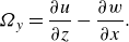 \begin{align} \Omega _y=\frac {\partial u}{\partial z} - \frac {\partial w}{ \partial x} . \end{align}
On the swimmers’ body, this vorticity can be viewed as two parts: the first $\partial u / \partial z$
part is due to the change in the axial velocity in the lateral direction (shear) and the second part
$\partial u / \partial z$
part is due to the change in the axial velocity in the lateral direction (shear) and the second part $\partial w / \partial x$
is generated by the body rotation. Inside the boundary layer adjacent to the body surface, we can use scaling analysis to approximate the parameters of (3.1) as
$\partial w / \partial x$
is generated by the body rotation. Inside the boundary layer adjacent to the body surface, we can use scaling analysis to approximate the parameters of (3.1) as
 \begin{align} u \sim U, \quad w \sim {fA}, \quad x \sim L, \quad z \sim \delta , \end{align}
where $\delta$
is the thickness of the boundary layer, which can be approximated by
$\delta$
is the thickness of the boundary layer, which can be approximated by $O(L/\sqrt {Re})$
, where
$O(L/\sqrt {Re})$
, where $O(\,)$
denotes order of magnitude, for a laminar layer. This is because in a laminar boundary layer, inertia and viscous forces are expected to be at least comparable, i.e. there must be a balance between
$O(\,)$
denotes order of magnitude, for a laminar layer. This is because in a laminar boundary layer, inertia and viscous forces are expected to be at least comparable, i.e. there must be a balance between $u \partial u / \partial x = O(U^2/L)$
and
$u \partial u / \partial x = O(U^2/L)$
and $\nu \partial ^2 u/ \partial z^2 = O(\nu U/ \delta ^2)$
terms in the Navier–Stokes (or Prandtl’s boundary layer) equations, implying
$\nu \partial ^2 u/ \partial z^2 = O(\nu U/ \delta ^2)$
terms in the Navier–Stokes (or Prandtl’s boundary layer) equations, implying $\delta =O(\nu L/U)^{1/2}$
. Substituting the above approximations into (3.1), dimensionless vorticity (along the
$\delta =O(\nu L/U)^{1/2}$
. Substituting the above approximations into (3.1), dimensionless vorticity (along the $y$
-axis) inside the boundary layer can be approximated as
$y$
-axis) inside the boundary layer can be approximated as
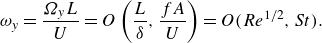 \begin{align} \omega _y =\frac {\Omega _yL}{U} = O \left ( \frac {L}{\delta}, \frac {{fA}}{U} \right ) = O(Re^{1/2}, St) . \end{align}
Readers are referred to appendix C of Akbarzadeh & Borazjani (Reference Akbarzadeh and Borazjani2019b
) for a more detailed derivation based on the skin friction of a 2-D undulating plate (Ehrenstein & Eloy Reference Ehrenstein and Eloy2013), which leads to $O(\sqrt {w/U}\sqrt {Re})=O(\sqrt {St}\sqrt {Re})$
for the shear component
$O(\sqrt {w/U}\sqrt {Re})=O(\sqrt {St}\sqrt {Re})$
for the shear component $\partial u/\partial z$
.
$\partial u/\partial z$
.
According to this dimensional analysis, the vorticity due to body rotation is of order $St$
, while the one due to shear in the boundary layer is of order
$St$
, while the one due to shear in the boundary layer is of order $\sqrt {Re}$
. During first cycles,
$\sqrt {Re}$
. During first cycles, $Re$
is much smaller and
$Re$
is much smaller and $St$
is much larger, when compared with those values at quasisteady (see figures 3
a and 3
b). Therefore, vorticity due to the body rotation
$St$
is much larger, when compared with those values at quasisteady (see figures 3
a and 3
b). Therefore, vorticity due to the body rotation $O(St)$
dominates the vorticity due to shear
$O(St)$
dominates the vorticity due to shear $O(\sqrt {Re})$
at the early cycles (figure 6
a,c,e). In contrast, at the quasisteady swimming,
$O(\sqrt {Re})$
at the early cycles (figure 6
a,c,e). In contrast, at the quasisteady swimming, $\sqrt {Re} \gg St$
, and consequently the vorticity due to shear
$\sqrt {Re} \gg St$
, and consequently the vorticity due to shear $O(\sqrt {Re})$
dominates the vorticity due to the body rotation
$O(\sqrt {Re})$
dominates the vorticity due to the body rotation $O(St)$
within the boundary layer for both kinematics, as observed in figure 6(b,d,f). Furthermore, the travelling wave kinematics exhibits a stronger vorticity in the boundary layer compared with the standing wave one because the
$O(St)$
within the boundary layer for both kinematics, as observed in figure 6(b,d,f). Furthermore, the travelling wave kinematics exhibits a stronger vorticity in the boundary layer compared with the standing wave one because the $Re$
of the lamprey with travelling wave is significantly higher. The higher shear in the boundary layer during quasisteady is also consistent with the viscous force
$Re$
of the lamprey with travelling wave is significantly higher. The higher shear in the boundary layer during quasisteady is also consistent with the viscous force $F_v$
trend increasing towards quasisteady state (figure 4
b) as the viscous force by definition is the integral of shear on the body.
$F_v$
trend increasing towards quasisteady state (figure 4
b) as the viscous force by definition is the integral of shear on the body.
In the derivation of the above scaling, no assumption was made about the outer flow of the boundary layer; that is, it remains valid for non-uniform outer flows (i.e. those with a non-zero streamwise pressure gradient) over curved bodies. Nevertheless, it was implicitly assumed that the boundary remains laminar and thin, which is a reasonable approximation because (i) the flow remains mostly attached to the body of the swimmers, and (ii) Reynolds number is below the threshold at which the boundary layer transitions to turbulence. Indeed, the flow remains attached on the windward side (exposed to the flow) from head to tail and may detach only near the tail on the leeward side (shielded from the flow), see figure 6. These assumptions, notwithstanding, do not affect the conclusion because the shear component is proportional to some power of $Re$
, e.g.
$Re$
, e.g. $O(Re^{1/5})$
for a turbulent boundary layer or
$O(Re^{1/5})$
for a turbulent boundary layer or $O(\sqrt {St}\sqrt {Re})$
for a 2-D undulating plate. Consequently, in the derived scaling, the power of
$O(\sqrt {St}\sqrt {Re})$
for a 2-D undulating plate. Consequently, in the derived scaling, the power of $Re$
may change from 1/2, but the main conclusion that ‘vorticity scales with shear (
$Re$
may change from 1/2, but the main conclusion that ‘vorticity scales with shear ( $Re$
) in quasisteady and body rotation (
$Re$
) in quasisteady and body rotation ( $St$
) at early cycles’ remains unchanged.
$St$
) at early cycles’ remains unchanged.
3.2. Pressure field and its scaling
Historically, pressure has received limited attention in aquatic swimming studies because (i) early theoretical works, based on potential theory, computed forces (lift $L$
) directly from circulation
$L$
) directly from circulation $\Gamma$
(vorticity) as
$\Gamma$
(vorticity) as $L=\rho U \Gamma$
and/or from added mass and (ii) experimental wake measurements that used control volume analysis ignored pressure on the boundaries, assuming boundaries were far enough from the body (Dabiri Reference Dabiri2005). Nevertheless, pressure is a key parameter for determining and analysing the energetics of swimming. According to (2.12), thrust force depends on pressure distribution on the swimmer’s surface. As illustrated in figure 1, the pressure difference between opposite sides of each segment of a thin body or tail generates a force normal to that segment. The projection of this force along the swimming direction determines the resultant thrust force.
$L=\rho U \Gamma$
and/or from added mass and (ii) experimental wake measurements that used control volume analysis ignored pressure on the boundaries, assuming boundaries were far enough from the body (Dabiri Reference Dabiri2005). Nevertheless, pressure is a key parameter for determining and analysing the energetics of swimming. According to (2.12), thrust force depends on pressure distribution on the swimmer’s surface. As illustrated in figure 1, the pressure difference between opposite sides of each segment of a thin body or tail generates a force normal to that segment. The projection of this force along the swimming direction determines the resultant thrust force.
To investigate the relation between pressure and thrust force generation, the pressure field on the same midplane as the vorticity visualisation is shown in figure 8 for the three swimmers during early cycles and at quasisteady state, corresponding to lower and higher $Re$
, respectively. Note that pressure in figure 8 is non-dimensionalised by
$Re$
, respectively. Note that pressure in figure 8 is non-dimensionalised by $\rho U_0^2$
which remains constant across different kinematics and swimming speeds. Therefore, the trend observed in non-dimensional pressure are representative of the dimensional trends as well. In all cases, pressure alternates between high and low magnitudes (positive to negative) from one side of the swimmer to the other and from head to tail. However, the magnitude of pressure varies depending on swimming speed (
$\rho U_0^2$
which remains constant across different kinematics and swimming speeds. Therefore, the trend observed in non-dimensional pressure are representative of the dimensional trends as well. In all cases, pressure alternates between high and low magnitudes (positive to negative) from one side of the swimmer to the other and from head to tail. However, the magnitude of pressure varies depending on swimming speed ( $Re$
) and kinematics. At early cycles (low
$Re$
) and kinematics. At early cycles (low $Re$
), the pressure difference across the body is significantly higher compared with the quasisteady state for all swimmers. Consequently, it can be expected that the thrust force decreases with increasing swimming speed (
$Re$
), the pressure difference across the body is significantly higher compared with the quasisteady state for all swimmers. Consequently, it can be expected that the thrust force decreases with increasing swimming speed ( $Re$
) as swimmers approach quasisteady state (see figures 8 and 4
b). At the quasisteady, the pressure difference across the body in the lamprey with a standing wave is significantly higher than in both the lamprey and the mackerel with the travelling wave (see figure 8
b,d,f). However, this higher pressure does not translate to greater thrust force due to unfavourable kinematics of standing waves. These observed trends – higher pressure at lower
$Re$
) as swimmers approach quasisteady state (see figures 8 and 4
b). At the quasisteady, the pressure difference across the body in the lamprey with a standing wave is significantly higher than in both the lamprey and the mackerel with the travelling wave (see figure 8
b,d,f). However, this higher pressure does not translate to greater thrust force due to unfavourable kinematics of standing waves. These observed trends – higher pressure at lower $Re$
and for standing waves – are counterintuitive as one might expect higher pressures at higher speeds. To explain these trends, a scaling analysis is performed, which is discussed in what follows.
$Re$
and for standing waves – are counterintuitive as one might expect higher pressures at higher speeds. To explain these trends, a scaling analysis is performed, which is discussed in what follows.
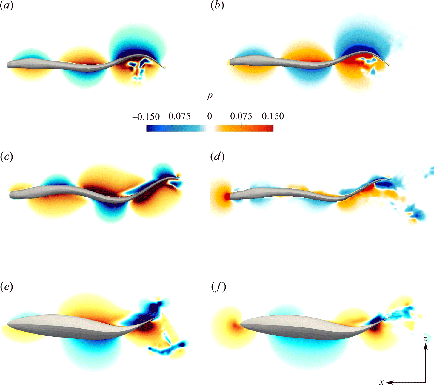
Figure 8. The non-dimensional pressure field on the horizontal midplane is shown for lamprey with standing (a,b) and travelling wave (c,d) and the mackerel with travelling wave (e,f). Panels (a,c,e) represent the first cycle of undulation, whereas panels (b,d,f) represent the quasisteady state. Pressure field is shown at the time instant when both swimmers produce the maximum thrust, i.e. $t/T=0.2$
for lamprey with travelling wave kinematics,
$t/T=0.2$
for lamprey with travelling wave kinematics, $t/T=0.0$
for lamprey with standing wave kinematics and
$t/T=0.0$
for lamprey with standing wave kinematics and $t/T=0.9$
for mackerel with travelling wave kinematics. The reference pressure is set based on the pressure at a corner of the computational domain, located far from the swimmer to ensure it remains unaffected by the swimmer’s motion.
$t/T=0.9$
for mackerel with travelling wave kinematics. The reference pressure is set based on the pressure at a corner of the computational domain, located far from the swimmer to ensure it remains unaffected by the swimmer’s motion.
Scaling analysis for the pressure is conducted by comparing pressure against its estimates from (i) the lift-based and (ii) the reactive mechanisms discussed in § 2.5. In what follows, a brief overview of the pressure generated by reactive and lift-based mechanisms and its connection to the normal acceleration and AoA, respectively, is presented. It is important to emphasise that both AoA (lift-based) and normal acceleration ( $a_n$
, reactive) depend strongly on the body undulations and the kinematics of the swimmer. These quantities vary dynamically in space and time, leading to spatially and temporally varying pressure fields along the swimmer’s body. This scaling analysis aims to clarify the contributions of each mechanism to the observed pressure distribution and thrust generation, offering insight into the dominant propulsion mechanisms under different kinematic conditions.
$a_n$
, reactive) depend strongly on the body undulations and the kinematics of the swimmer. These quantities vary dynamically in space and time, leading to spatially and temporally varying pressure fields along the swimmer’s body. This scaling analysis aims to clarify the contributions of each mechanism to the observed pressure distribution and thrust generation, offering insight into the dominant propulsion mechanisms under different kinematic conditions.
For the reactive propulsion mechanism, when the swimmer undulates, the body undergoes lateral displacements $h(x,t)$
and each thin cross-section of the body perpendicular to the swimming direction pushes a vertical slice of water laterally and accelerates adjacent fluid particles (Lighthill Reference Lighthill1960) (figure 1
a). According to the elongated body theory (Lighthill Reference Lighthill1960; Wu Reference Wu1961), the fluid is accelerated laterally to a velocity
$h(x,t)$
and each thin cross-section of the body perpendicular to the swimming direction pushes a vertical slice of water laterally and accelerates adjacent fluid particles (Lighthill Reference Lighthill1960) (figure 1
a). According to the elongated body theory (Lighthill Reference Lighthill1960; Wu Reference Wu1961), the fluid is accelerated laterally to a velocity $w$
by both the lateral velocity of the body
$w$
by both the lateral velocity of the body $W=\partial h/ \partial t$
and the angle of the body against the swimming direction (
$W=\partial h/ \partial t$
and the angle of the body against the swimming direction ( $U \partial h/\partial x$
), see § 2.5. As a result of this fluid acceleration, pressure increases on one side of body segment and decreases on the opposite side, similar to the pressure generated by a paddle moving through water (figure 1
a). The high-pressure side corresponds to the region where the acceleration of fluid particles
$U \partial h/\partial x$
), see § 2.5. As a result of this fluid acceleration, pressure increases on one side of body segment and decreases on the opposite side, similar to the pressure generated by a paddle moving through water (figure 1
a). The high-pressure side corresponds to the region where the acceleration of fluid particles $\textrm {d} w/\textrm {d}t$
and the outward normal vector of the body
$\textrm {d} w/\textrm {d}t$
and the outward normal vector of the body $\boldsymbol {n}$
point in the same direction. Conversely, the low-pressure side occurs where these directions oppose each other. Consequently, the acceleration in the normal direction (
$\boldsymbol {n}$
point in the same direction. Conversely, the low-pressure side occurs where these directions oppose each other. Consequently, the acceleration in the normal direction ( $a_n$
) of the body surface (as defined in (2.9)), is expected to scale with pressure according to the theory (Lighthill Reference Lighthill1960; Wu Reference Wu1961) if the swimmer utilises the reactive mechanism for propulsion.
$a_n$
) of the body surface (as defined in (2.9)), is expected to scale with pressure according to the theory (Lighthill Reference Lighthill1960; Wu Reference Wu1961) if the swimmer utilises the reactive mechanism for propulsion.
According to the lift-based propulsion mechanism, when the fluid flows over a tangential segment of the body, such as the caudal fin shown in figure 1(b), a lift force generated as the result of pressure difference across that segment. This pressure difference (lift force) is proportional to the circulation of flow around the segment, as described by the Kutta–Joukowski theorem. The circulation itself depends on the AoA. Therefore, pressure projected on the body is expected to scale with the AoA if the swimmer primarily utilises the lift-based propulsion mechanism.
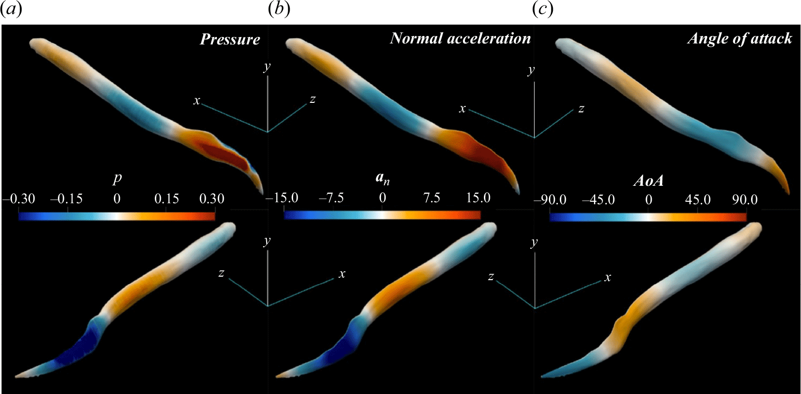
Figure 9. Comparison of non-dimensional pressure (a), normal acceleration (b) and AoA (c) on the both sides of the surface of lamprey with standing wave undulations at $t/T=0$
. With the exception of some differences at the edges of the lamprey, surface pressure closely follows the normal acceleration
$t/T=0$
. With the exception of some differences at the edges of the lamprey, surface pressure closely follows the normal acceleration $a_n$
. In contrast, there is no clear correlation between surface pressure and the AoA
$a_n$
. In contrast, there is no clear correlation between surface pressure and the AoA $\alpha$
. See Supplementary video 1.
$\alpha$
. See Supplementary video 1.
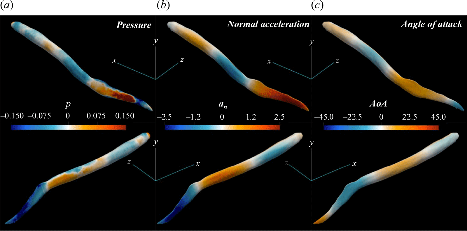
Figure 10. Comparison of non-dimensional pressure (a), normal acceleration (b) and AoA (c) on both sides of the surface of lamprey with travelling wave undulations at $t/T=0.2$
. With the exception of some differences at the edges of the lamprey, surface pressure closely follows the normal acceleration
$t/T=0.2$
. With the exception of some differences at the edges of the lamprey, surface pressure closely follows the normal acceleration $a_n$
. In contrast, there is no clear correlation between surface pressure and the AoA
$a_n$
. In contrast, there is no clear correlation between surface pressure and the AoA $\alpha$
. See Supplementary video 2.
$\alpha$
. See Supplementary video 2.
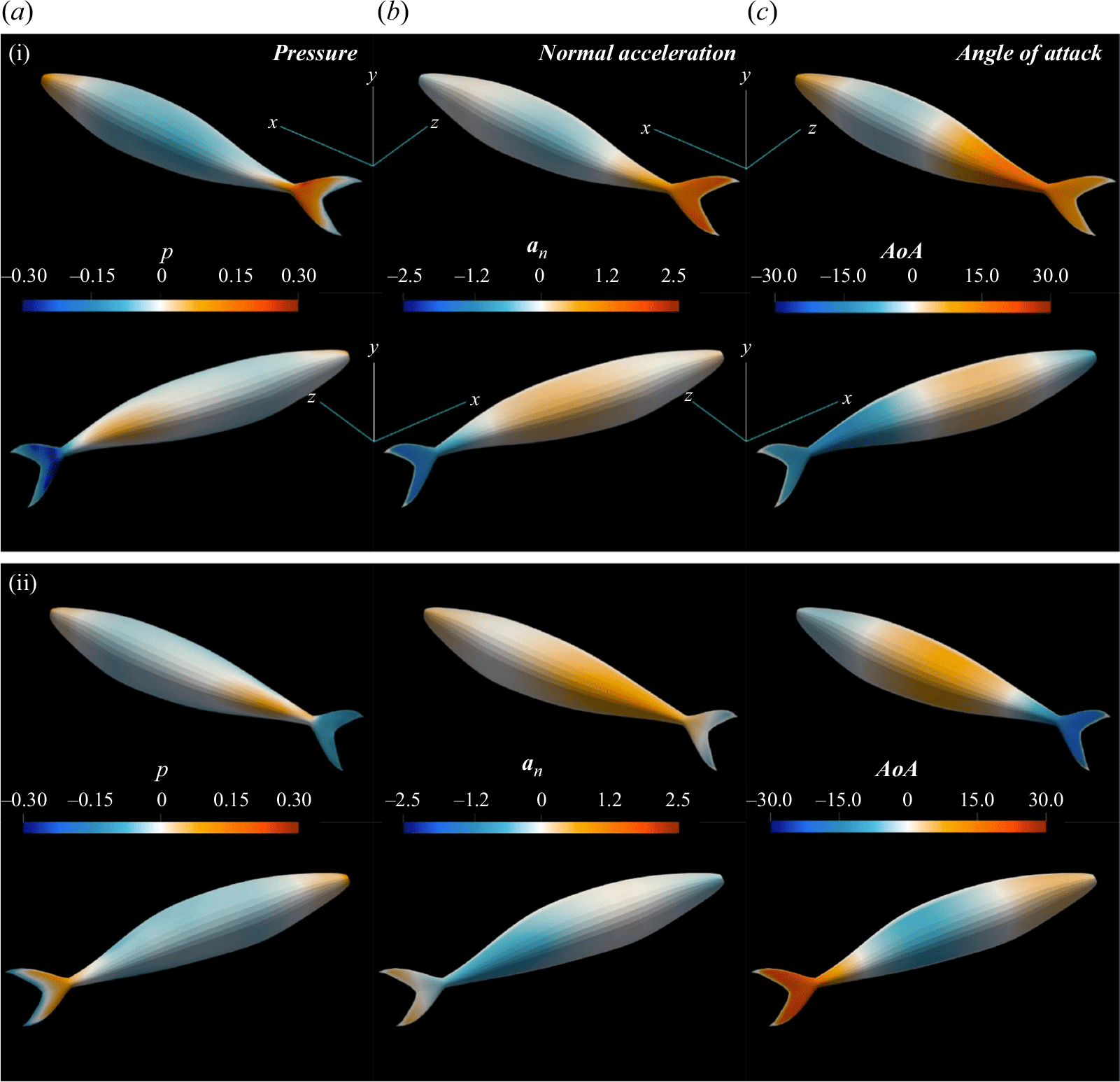
Figure 11. Comparison of non-dimensional pressure (a), normal acceleration (b) and AoA (c) on both sides of the surface of mackerel with travelling wave undulations at $t/T=0.9$
(i) and
$t/T=0.9$
(i) and $t/T=0.6$
(ii), respectively. Surface pressure is proportional to the normal acceleration
$t/T=0.6$
(ii), respectively. Surface pressure is proportional to the normal acceleration $a_n$
at some instants (i) and to the AoA at some other (ii). See Supplementary video 3.
$a_n$
at some instants (i) and to the AoA at some other (ii). See Supplementary video 3.
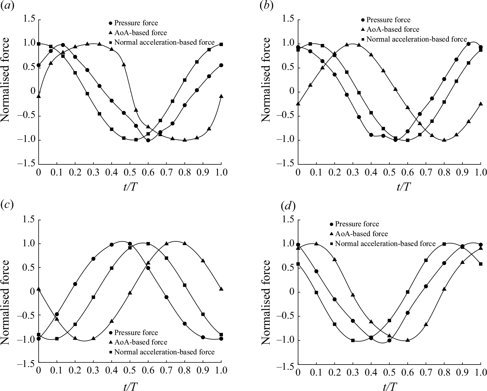
Figure 12. Comparison of the net lateral force by pressure, normal acceleration and AoA for the (a) Lamprey with standing wave, (b) Lamprey with travelling wave, (c) body of the mackerel and (d) tail of the mackerel.
To analyse the correlation between pressure and reactive/lift-based mechanisms, the pressure, normal acceleration of fluid and AoA on the surface of swimmers are shown in figure 9 (Supplementary video 1) for the lamprey with standing wave undulation, in figure 10 (Supplementary video 2) for the lamprey with travelling wave undulation and in figure 11 (Supplementary video 3) for the mackerel with travelling wave undulation at quasisteady state. The figures 9, 10 and figure 11(ai,bi,ci) correspond to the time instants of maximum thrust generation. Figure 11(aii,bii,cii) represent a different time instant chosen specifically to better illustrate the correlation between pressure and AoA for the mackerel with travelling wave undulation. It can be observed that pressure, normal acceleration and AoA generally increase from head to tail across all swimmers. This trend arises due to the higher amplitude of body undulations in the posterior region. In the anterior region of the body, the lateral velocity is relatively low. Consequently, the AoA is primarily determined by the angle of a body segment relative to the streamwise direction. In this region, AoA is positive on the pressure side where the flow impinges on the body and it is negative on the suction side. In the posterior region, lateral velocity becomes high, and its contribution to the relative velocity of a body segment can vary drastically. As a result, AoA in this region is influenced by both the segment angle relative to the streamwise direction and the lateral velocity of the body segment. For both lampreys (figures 9 and 10) it can be observed that, except near some of the edges, pressure distribution on the swimmers’ body better scales with the fluid acceleration along the normal direction rather than AoA (2.9). For the mackerel, however, as observed in figure 11, the pressure scales with AoA at some instants of a cycle but acceleration at some other instants. Notably, the mackerel produces a net thrust force when pressure correlates with both acceleration and AoA as illustrated in the figure 11(ai,bi,ci). When the pressure field only correlates with either normal acceleration or AoA, the mackerel produces a net drag force. This observation suggest that the reactive (added mass) and lift-based (circulatory) forces are of similar order of magnitude on the mackerel tail, highlighting the critical interplay between these two mechanisms for effective propulsion in carangiform swimming.
To quantify the correlations between pressure, normal acceleration and AoA, the net lateral force resulting from each quantity is computed by integrating them over the swimmer’s surface at different instants in a swimming cycle., e.g. $F_{p_z}(t)=-\int p n_z\ {\textrm{d}}A$
. The net lateral force by these quantities is normalised because the interest is in their phase difference rather than their magnitude. The normalised lateral forces due to these quantities are plotted in figure 12 for lamprey with standing wave (figure 12
a), lamprey with travelling wave (figure 12
b), the body (figure 12
c) and tail (figure 12
d) of the mackerel. Each plot shows two peaks per cycle, one positive and one negative, corresponding to the motion of the tail in positive and negative lateral directions during one tailbeat cycle. The phase difference between the net forces can be estimated by comparing the location of the peaks of each curve. The correlations previously discussed are further supported by the results shown in figure 12. For both lampreys (standing wave (figure 12
a) and travelling wave (figure 12
b), the pressure-based force shows a stronger correlation with normal acceleration than with AoA, as the phase difference between the pressure force and normal acceleration force is approximately
$F_{p_z}(t)=-\int p n_z\ {\textrm{d}}A$
. The net lateral force by these quantities is normalised because the interest is in their phase difference rather than their magnitude. The normalised lateral forces due to these quantities are plotted in figure 12 for lamprey with standing wave (figure 12
a), lamprey with travelling wave (figure 12
b), the body (figure 12
c) and tail (figure 12
d) of the mackerel. Each plot shows two peaks per cycle, one positive and one negative, corresponding to the motion of the tail in positive and negative lateral directions during one tailbeat cycle. The phase difference between the net forces can be estimated by comparing the location of the peaks of each curve. The correlations previously discussed are further supported by the results shown in figure 12. For both lampreys (standing wave (figure 12
a) and travelling wave (figure 12
b), the pressure-based force shows a stronger correlation with normal acceleration than with AoA, as the phase difference between the pressure force and normal acceleration force is approximately $+\pi /8$
but with AoA is approximately
$+\pi /8$
but with AoA is approximately $+\pi /2$
. The small phase difference between the pressure and normal acceleration lateral forces can be attributed to the differences observed at the edges (will be discussed later) and the anterior region, where the body undulations, and consequently acceleration, are minimal. For the mackerel body (figure 12
c) and tail (figure 12
d), however, the pressure-based lateral force exhibits a phase difference of approximately
$+\pi /2$
. The small phase difference between the pressure and normal acceleration lateral forces can be attributed to the differences observed at the edges (will be discussed later) and the anterior region, where the body undulations, and consequently acceleration, are minimal. For the mackerel body (figure 12
c) and tail (figure 12
d), however, the pressure-based lateral force exhibits a phase difference of approximately $-\pi /3$
with normal acceleration and it shows a phase difference of approximately
$-\pi /3$
with normal acceleration and it shows a phase difference of approximately $+\pi /3$
with AoA-based force. This suggests that the pressure distribution on the mackerel is influenced by both reactive (normal acceleration) and lift-based (AoA) mechanisms.
$+\pi /3$
with AoA-based force. This suggests that the pressure distribution on the mackerel is influenced by both reactive (normal acceleration) and lift-based (AoA) mechanisms.
For lampreys, the higher pressure difference for standing waves and at lower swimming speeds in figure 8 can be explained based on the scaling with normal acceleration, as observed in figures 9 and 10. In the standing wave swimmer, due to unfavourable body alignment with the swimming direction, pressure difference across the body does not contribute towards thrust force, as much as it does for the travelling wave, resulting in a slower swimming speed and high lateral acceleration $\textrm {d} w/\textrm {d}t$
, and consequently higher pressure difference. Similarly, the swimmer with a travelling wave creates much higher pressure at lower swimming speeds (lower
$\textrm {d} w/\textrm {d}t$
, and consequently higher pressure difference. Similarly, the swimmer with a travelling wave creates much higher pressure at lower swimming speeds (lower $Re$
) because
$Re$
) because $\textrm {d} w/\textrm {d}t$
for a given body undulation decreases as
$\textrm {d} w/\textrm {d}t$
for a given body undulation decreases as $U$
is increased. Indeed, it can be theoretically shown that the order of lateral fluid acceleration
$U$
is increased. Indeed, it can be theoretically shown that the order of lateral fluid acceleration $\textrm {d} w/\textrm {d}t$
for travelling wave kinematics is
$\textrm {d} w/\textrm {d}t$
for travelling wave kinematics is $O( 4 \pi ^2 a(V- U)^2/{\lambda ^2} )$
where
$O( 4 \pi ^2 a(V- U)^2/{\lambda ^2} )$
where $V$
is dimensionless wave speed, see (B3) and appendix B for the derivation. Because
$V$
is dimensionless wave speed, see (B3) and appendix B for the derivation. Because $U\lt V$
for self-propulsion, the order of
$U\lt V$
for self-propulsion, the order of $\textrm {d} w/\textrm {d}t$
will decrease as
$\textrm {d} w/\textrm {d}t$
will decrease as $U$
increases and approaches
$U$
increases and approaches $V$
. This can also be observed heuristically in figure 1(a). The upwards acceleration of the shown segment accelerates the fluid particle upwards, whereas the forward motion of the shown segment accelerates the fluid particle downwards, opposite to the upward acceleration of the segment, resulting in the reduction of the upwards acceleration of the fluid particle and consequently the pressure difference. For the mackerel, similarly, the higher pressures can be explained by the pressure scaling with both AoA and normal acceleration. The same argument as lamprey for lower fluid acceleration at higher velocities can be made for mackerel. Similarly, it can be argued that the AoA decreases as the swimming speed
$V$
. This can also be observed heuristically in figure 1(a). The upwards acceleration of the shown segment accelerates the fluid particle upwards, whereas the forward motion of the shown segment accelerates the fluid particle downwards, opposite to the upward acceleration of the segment, resulting in the reduction of the upwards acceleration of the fluid particle and consequently the pressure difference. For the mackerel, similarly, the higher pressures can be explained by the pressure scaling with both AoA and normal acceleration. The same argument as lamprey for lower fluid acceleration at higher velocities can be made for mackerel. Similarly, it can be argued that the AoA decreases as the swimming speed $U$
increases. Based on figure 1(b), the angle that the body makes with the swimming direction
$U$
increases. Based on figure 1(b), the angle that the body makes with the swimming direction $\theta =\tan ^{-1}( \partial h / \partial x)$
does not change with the swimming speed. However, the relative velocity angle with the swimming direction
$\theta =\tan ^{-1}( \partial h / \partial x)$
does not change with the swimming speed. However, the relative velocity angle with the swimming direction $\gamma = \tan ^{-1}(- ({1}/{U})\partial h / \partial t)$
decreases as
$\gamma = \tan ^{-1}(- ({1}/{U})\partial h / \partial t)$
decreases as $U$
increases. Consequently, AoA (
$U$
increases. Consequently, AoA ( $\alpha =\gamma - \theta$
) will also decrease.
$\alpha =\gamma - \theta$
) will also decrease.
In the above analysis, the streamwise acceleration ${\textrm{d}}U/{\textrm{d}}t$
of the swimmers, which is non-zero during early cycles, has been neglected. This is justified if the streamwise acceleration is much lower than the lateral acceleration
${\textrm{d}}U/{\textrm{d}}t$
of the swimmers, which is non-zero during early cycles, has been neglected. This is justified if the streamwise acceleration is much lower than the lateral acceleration $a_n$
. To determine the streamwise acceleration
$a_n$
. To determine the streamwise acceleration ${\textrm{d}}U/{\textrm{d}}t$
, the slope of the velocity curve shown in figure 3(a) needs to be computed. It can be observed that the mackerel has the highest streamwise acceleration (slope of the curve) among the swimmers and its acceleration is highest during early cycles (figure 3
a). In fact, the mackerel reaches
${\textrm{d}}U/{\textrm{d}}t$
, the slope of the velocity curve shown in figure 3(a) needs to be computed. It can be observed that the mackerel has the highest streamwise acceleration (slope of the curve) among the swimmers and its acceleration is highest during early cycles (figure 3
a). In fact, the mackerel reaches $U$
= 0.146 at end of first cycle, i.e. resulting in a mean non-dimensional streamwise acceleration of approximately
$U$
= 0.146 at end of first cycle, i.e. resulting in a mean non-dimensional streamwise acceleration of approximately ${\textrm{d}}U/{\textrm{d}}t \approx U/T$
= 0.146/0.6667 = 0.22 where
${\textrm{d}}U/{\textrm{d}}t \approx U/T$
= 0.146/0.6667 = 0.22 where $T=2 a_{max}/St_0=0.6667$
is the non-dimensional period. The normal acceleration
$T=2 a_{max}/St_0=0.6667$
is the non-dimensional period. The normal acceleration $a_n$
in the early cycles, computed according to (B2), is of order
$a_n$
in the early cycles, computed according to (B2), is of order $O( 4 \pi ^2 a/T^2)\approx$
8.88 assuming
$O( 4 \pi ^2 a/T^2)\approx$
8.88 assuming $U \approx 0$
during the first cycle. This indicates that the lateral acceleration
$U \approx 0$
during the first cycle. This indicates that the lateral acceleration $a_n$
is much higher than the streamwise acceleration, even during early cycles. Therefore, streamwise acceleration can be safely ignored in the analysis relative to the lateral acceleration. Consequently, the added mass force predominantly arises from the lateral acceleration and not from the streamwise component. The relatively low streamwise acceleration observed here can be attributed to the prescribed body motion of the swimmers, which is optimised for typical cruising motion rather than fast-start manoeuvers. In nature, fish employ a distinct body motion pattern for fast starts, characterised by higher streamwise accelerations and a different undulation profile (Webb Reference Webb1978; Borazjani et al. Reference Borazjani, Sotiropoulos, Tytell and Lauder2012).
$a_n$
is much higher than the streamwise acceleration, even during early cycles. Therefore, streamwise acceleration can be safely ignored in the analysis relative to the lateral acceleration. Consequently, the added mass force predominantly arises from the lateral acceleration and not from the streamwise component. The relatively low streamwise acceleration observed here can be attributed to the prescribed body motion of the swimmers, which is optimised for typical cruising motion rather than fast-start manoeuvers. In nature, fish employ a distinct body motion pattern for fast starts, characterised by higher streamwise accelerations and a different undulation profile (Webb Reference Webb1978; Borazjani et al. Reference Borazjani, Sotiropoulos, Tytell and Lauder2012).
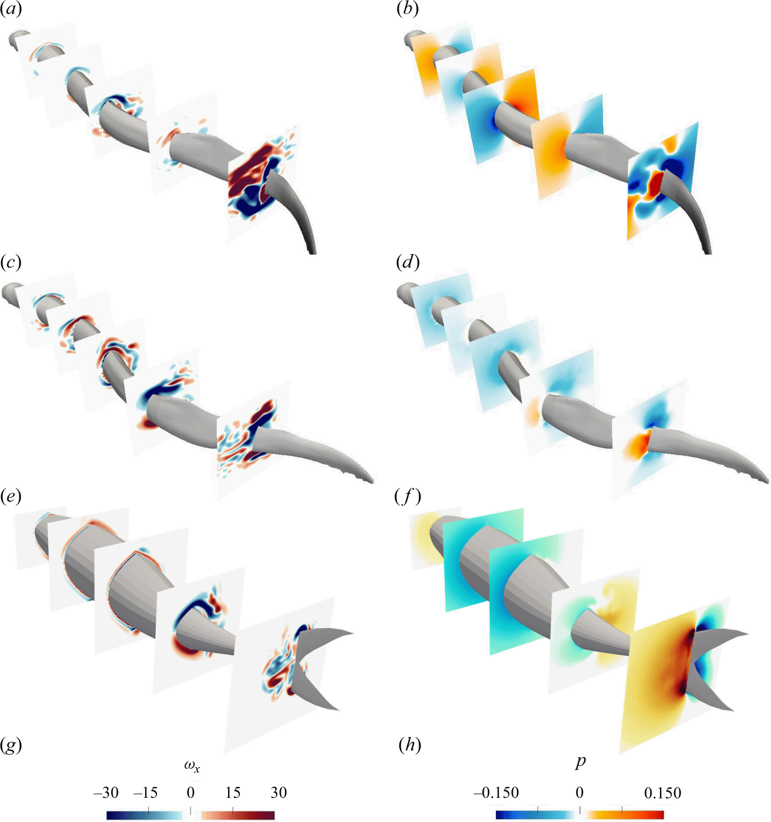
Figure 13. Comparison of non-dimensional out-of-plane vorticity (a,c,e) and pressure fields (b,d,f) at the quasisteady at the time instant of maximum thrust, i.e. $t/T$
= 0.2, 0 and 0.9 for lamprey with standing wave kinematics, lamprey with travelling wave kinematics and mackerel with travelling wave kinematics, respectively.
$t/T$
= 0.2, 0 and 0.9 for lamprey with standing wave kinematics, lamprey with travelling wave kinematics and mackerel with travelling wave kinematics, respectively.
According to the elongated body theory (Lighthill Reference Lighthill1960; Wu Reference Wu1961) or the lift-force theory, pressure distribution on the body surface, whether arising from lateral acceleration or AoA, does not predict any variations along the vertical (dorsoventral or $y$
-) direction. However, visualisations of surface pressures clearly show vertical variations, especially near the edges in the posterior part of the body for the lamprey and near the tail for the mackerel (see figures 9–11). These vertical variations are likely due to the formation of edge vortices, which are visualised in figure 13 using out-plane-vorticity at cross-sections perpendicular to the swimming direction. Similar edge vortices have been previously observed in fish larvae (Li et al. Reference Li, Müller, van Leeuwen and Liu2016) and mackerel tails (Borazjani & Daghooghi Reference Borazjani and Daghooghi2013).
$y$
-) direction. However, visualisations of surface pressures clearly show vertical variations, especially near the edges in the posterior part of the body for the lamprey and near the tail for the mackerel (see figures 9–11). These vertical variations are likely due to the formation of edge vortices, which are visualised in figure 13 using out-plane-vorticity at cross-sections perpendicular to the swimming direction. Similar edge vortices have been previously observed in fish larvae (Li et al. Reference Li, Müller, van Leeuwen and Liu2016) and mackerel tails (Borazjani & Daghooghi Reference Borazjani and Daghooghi2013).
The edge vortices typically form due to the pressure differences across the edge, which arise from fluid acceleration during undulations. This phenomenon is analogous to tip vortices observed on aeroplane wings. A leading-edge vortex forms when flow separates at the leading edge but subsequently reattaches before reaching the trailing edge. This vortex formation generally reduces the pressure difference across the tip/edge. However, if edge vortices remain near the edge and shift slightly towards the low-pressure side, they can enhance the low-pressure region on that side (Li et al. Reference Li, Müller, van Leeuwen and Liu2016). This results in the formation of a thin low-pressure zone around the edge on the high-pressure side of swimmers. The formation of the leading-edge vortex is also known to increase circulation around the tail or posterior segment, thereby enhancing the lift-based force generation (Borazjani & Daghooghi Reference Borazjani and Daghooghi2013).
4. Conclusion
Traditionally, anguilliform and carangiform propulsion have been interpreted through two distinct mechanisms: the reaction force mechanism (added mass mechanism), which arises from accelerating the surrounding fluid, and the lift-based mechanism, which depends on the circulation of fluid over the tail. These mechanisms are typically associated with anguilliform (reactive force) and carangiform (lift-based force) swimmers, respectively. However, there is limited data supporting these interpretations, largely because of the challenges involved in decomposing forces/pressure into components that can be clearly attributed to either mechanism. Although it is well established that the lift-based mechanism cannot generate thrust under no-flow conditions (Borazjani & Sotiropoulos Reference Borazjani and Sotiropoulos2008, Reference Borazjani and Sotiropoulos2010), at high Reynolds numbers, both lift-based (steady) and added mass (unsteady) mechanisms can simultaneously contribute to thrust generation. While thrust can be measured directly, accurately decomposing it into reactive (added mass) and lift-based components remains a significant challenge. Consequently, the dominant mechanism for anguilliform and carangiform swimmers has yet to be conclusively elucidated. One of the primary contributions of this study is the establishment of correlations between pressure distributions (responsible for thrust generation) and key parameters that represent the reactive (normal acceleration) and lift-based (AoA) mechanisms. These correlations provide new insights into the relative contributions of these mechanisms across different swimming kinematics and conditions and offer a framework for understanding the hydrodynamic forces driving anguilliform and carangiform propulsion more comprehensively.
Whenever fluid is accelerated by a propulsive element, a high-pressure region is created on the side where the surface normal aligns with the direction of fluid acceleration, while a low-pressure region forms on the opposite side (figure 1). This fundamental principle has been well-recognised in early theories of aquatic locomotion, particularly in the works of Lighthill (Reference Lighthill1960) and Wu (Reference Wu1961). In equation (24) of Wu (Reference Wu1961), it is shown that the pressure distribution on the sides of an undulating plate is equal and opposite, with one side exhibiting positive pressure and the other side negative pressure. This symmetry arises directly from the acceleration imparted to the fluid by the undulating body segment.
Through self-propelled, large-eddy simulations conducted at realistic swimming conditions (Reynolds and Strouhal numbers), we have demonstrated that, in lampreys, the high and low pressures in the fluid near the body scale with the normal acceleration of the fluid particles and not just the lateral acceleration of the body. The acceleration of fluid particles in this context, illustrated in figure 1(a), is a combination of the lateral acceleration of the body (local acceleration) and the acceleration from fluid particles being pushed laterally by the body as it swims at a constant speed and at an angle relative to the swimming direction (convective acceleration).
For lift-based mechanisms (illustrated in figure 1 b), fluid particle acceleration arises primarily from convective acceleration. This acceleration occurs as fluid particles are pushed laterally by the body or tail as it oscillates at an angle to the swimming direction. The resulting motion generates a high-pressure region on one side of the tail segment and a low-pressure region on the opposite side. In the case of the mackerel, our simulations show that the pressure scales with both the normal acceleration and AoA. In fact, the thrust is maximised when the pressure correlates well with both the AoA and the normal acceleration.
These scalings explain why pressure near the body, and consequently thrust force, decreases as swimming speed increases. This trend arises because both fluid acceleration and the AoA decrease with increasing swimming velocity. For the normal acceleration, the acceleration due to body angle $U \partial h / \partial x$
, which increases with the swimming speed, counteracts the body acceleration
$U \partial h / \partial x$
, which increases with the swimming speed, counteracts the body acceleration $\partial h / \partial t$
, thereby reducing the normal acceleration. The AoA also decreases as the swimming speed
$\partial h / \partial t$
, thereby reducing the normal acceleration. The AoA also decreases as the swimming speed $U$
increases because the angle of the relative velocity
$U$
increases because the angle of the relative velocity $\theta = \tan ^{-1}(- ({1}/{U})\partial h / \partial t)$
decreases with
$\theta = \tan ^{-1}(- ({1}/{U})\partial h / \partial t)$
decreases with $U$
(figure 1
b).
$U$
(figure 1
b).
Our results are consistent with the theory (Lighthill Reference Lighthill1960; Wu Reference Wu1961), demonstrating that swimmers employing travelling wave kinematics achieve significantly higher swimming speeds compared with those using standing wave kinematics. Additionally, the streamlines observed in our simulations (figure 6) are qualitatively similar to the experiments (Tytell & Lauder Reference Tytell and Lauder2004). During the early cycles, when the Reynolds number is low and the Strouhal number is high, the vorticity field in the simulations (figure 6
a,c,e) follows the body rotation because the vorticity generated by body rotation dominates over shear vorticity. As the swimmer accelerates and $Re$
increases while
$Re$
increases while $St$
decreases, the system eventually stabilises at a quasisteady state (figure 3). In this state, the vorticity (figure 6
b,d,f) no longer follows the body rotation due to the dominance of shear vorticity. This observation aligns well with the scaling analysis, which indicates that the shear vorticity (shear rate) scales with
$St$
decreases, the system eventually stabilises at a quasisteady state (figure 3). In this state, the vorticity (figure 6
b,d,f) no longer follows the body rotation due to the dominance of shear vorticity. This observation aligns well with the scaling analysis, which indicates that the shear vorticity (shear rate) scales with $\sqrt Re$
assuming laminar boundary layer (otherwise some power of
$\sqrt Re$
assuming laminar boundary layer (otherwise some power of $Re$
), suggesting that (i) the vorticity in the boundary layer and (ii) viscous drag (viscosity times shear rate) both increase with swimming velocity.
$Re$
), suggesting that (i) the vorticity in the boundary layer and (ii) viscous drag (viscosity times shear rate) both increase with swimming velocity.
Our findings indicates that efficient swimming requires minimising the pressure difference across the body, a condition clearly observed in the travelling wave kinematics (figure 8
d and 8f) compared with the standing wave kinematics (figure 8
b). While the pressure difference must be sufficient to overcome viscous drag, keeping it as small as possible reduces the power required for propulsion, as power is proportional to the product of pressure difference and the lateral velocity of the body. This principle aligns with Lighthill’s assertion that for efficient thrust production, the acceleration of fluid particles $w$
should be small relative to the acceleration of body
$w$
should be small relative to the acceleration of body $W$
, but still positively correlated with it (Lighthill Reference Lighthill1960) (figure 1
a). This is a restrictive condition and Lighthill (Reference Lighthill1960) pointed out that a standing wave theoretically achieves a maximum Froude efficiency of
$W$
, but still positively correlated with it (Lighthill Reference Lighthill1960) (figure 1
a). This is a restrictive condition and Lighthill (Reference Lighthill1960) pointed out that a standing wave theoretically achieves a maximum Froude efficiency of $\frac {1}{2}$
, much lower than that of a travelling wave. Lighthill (Reference Lighthill1960) states that ‘this is doubtless why fish do not normally attempt to swim by causing their bodies to execute the rather simple movements of a standing wave’. Recent applications of travelling waves in flow control further highlight their superior performance over standing waves (Akbarzadeh & Borazjani Reference Akbarzadeh and Borazjani2020; Ogunka et al. Reference Ogunka, Akbarzadeh and Borazjani2023).
$\frac {1}{2}$
, much lower than that of a travelling wave. Lighthill (Reference Lighthill1960) states that ‘this is doubtless why fish do not normally attempt to swim by causing their bodies to execute the rather simple movements of a standing wave’. Recent applications of travelling waves in flow control further highlight their superior performance over standing waves (Akbarzadeh & Borazjani Reference Akbarzadeh and Borazjani2020; Ogunka et al. Reference Ogunka, Akbarzadeh and Borazjani2023).
Supplementary movies.
Supplementary movies are available at https://doi.org/10.1017/jfm.2025.251.
Acknowledgements
The computational resources provided by high-performance computing institute (HPRC) at Texas A&M University. We are grateful to Professor Smits (Princeton University) for providing the lamprey morphology data from the CT data of Professor Fish (West Chester University).
Declaration of interests
The authors report no conflict of interest.
Appendix A. Surface pressure and normal acceleration
At high Reynolds numbers, the flow can be approximated as inviscid and irrotational outside the boundary layer. Under these conditions, the fluid behaves as an ideal flow, and the effects of viscosity can be neglected except within the boundary layer region adjacent to the body surface. When a body accelerates in such an ideal flow, it imparts acceleration to the adjacent fluid particles, creating a reaction force known as the ‘added mass’ force. This force represents the inertia of the surrounding fluid that the body must overcome as it moves. As an example, consider a circular cylinder of radius $R$
moving with a lateral velocity
$R$
moving with a lateral velocity $w$
through a fluid of density
$w$
through a fluid of density $\rho$
(see figure 14). The associated pressure distribution
$\rho$
(see figure 14). The associated pressure distribution $p$
on this circular cylinder can be found from the unsteady Bernoulli equation, given by
$p$
on this circular cylinder can be found from the unsteady Bernoulli equation, given by
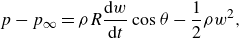 \begin{align} p-p_{\infty }= \rho R \frac {\textrm {d}w}{\textrm {d}t} \cos \theta -\frac {1}{2} \rho w^2 , \end{align}
where $p_{\infty }$
is pressure far from the cylinder and
$p_{\infty }$
is pressure far from the cylinder and $\cos(\theta )$
represents the outward normal
$\cos(\theta )$
represents the outward normal $\mathbf{n}$
on the cylinder. Therefore, the pressure difference between two sides of a cross-section can be written as
$\mathbf{n}$
on the cylinder. Therefore, the pressure difference between two sides of a cross-section can be written as
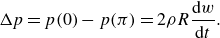 \begin{align} \Delta p = p(0)-p(\pi )=2 \rho R \frac {\textrm {d}w}{\textrm {d}t} . \end{align}
It can be observed, based on this equation, that when accelerating from centre line $\textrm {d}w/\textrm {d}t\gt 0$
, pressure on the right-hand side,
$\textrm {d}w/\textrm {d}t\gt 0$
, pressure on the right-hand side, $p(0)$
, is higher than the opposite side. Conversely, when decelerating
$p(0)$
, is higher than the opposite side. Conversely, when decelerating $\textrm {d}w/\textrm {d}t\lt 0$
, pressure on the left-hand side,
$\textrm {d}w/\textrm {d}t\lt 0$
, pressure on the left-hand side, $p(\pi )$
, is higher than that of the right-hand side.
$p(\pi )$
, is higher than that of the right-hand side.
In such an ideal flow and for an undulatory mode of propulsion, the elongated body theory (Lighthill Reference Lighthill1960) estimates the performance of a slender fish by considering the added mass of small amplitude lateral motions. During the motion of the body along the lateral direction, each infinitesimal cross-section of the body, perpendicular to the swimmer’s centreline, is considered as a thin cylinder and pushes a vertical slice of water laterally and accelerates adjacent fluid particles (Lighthill Reference Lighthill1960). It generates a pressures difference on opposite sides of any infinitesimal element similar to the cylinder example. Nevertheless, the Bernoulli equation relating the pressure to the acceleration of cross-sections is more complicated than (A1), see equation (A12) of Lighthill (Reference Lighthill1960).
Appendix B. Effect of swimming speed on normal acceleration and thrust
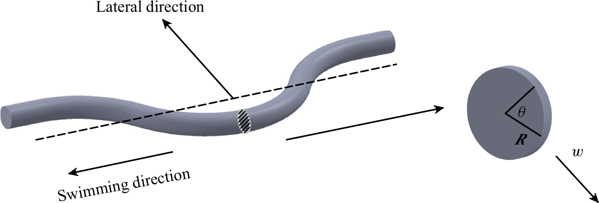
Figure 14. A schematic for an undulatory circular cylinder moving through a fluid. The pressure on the body surface is correlated to the lateral acceleration as the unsteady Bernoulli equation states.
For a given undulation kinematics and frequency, the fluid lateral velocity and acceleration is a function of swimming speed as demonstrated in elongated body theory (Lighthill Reference Lighthill1960). To give a quantitative example, let us consider a simpler kinematics for both travelling and standing waves with constant amplitude as follows:
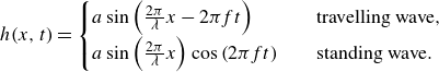 \begin{align} h(x,t) = \begin{cases} a\sin \left ( \frac {2\pi }{\lambda } x- 2 \pi f t\right ) & \quad \text {travelling wave}, \\[3pt] a \sin \left ( \frac {2\pi }{\lambda } x \right ) \cos \left ( 2\pi f t\right ) & \quad \text {standing wave}. \\ \end{cases} \end{align}
Then acceleration according to (2.8) is
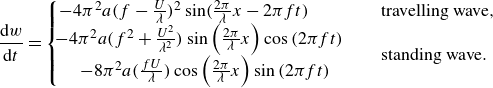 \begin{align} { \frac {\textrm {d} w}{\textrm {d}t} = \begin{cases} -4 \pi ^2 a (f- \frac {U}{\lambda })^2 \sin (\frac {2 \pi }{\lambda } x-2 \pi f t) & \quad \text {travelling wave},\\ {\begin{array}{l}\!\!-4 \pi ^2 a (f^2+ \frac {U^2}{\lambda ^2})\sin \left ( \frac {2\pi }{\lambda }x\right )\cos \left ( 2\pi f t\right )\\ \quad-8 \pi ^2 a (\frac {fU}{\lambda })\cos \left ( \frac {2\pi }{\lambda }x\right )\sin \left ( 2\pi f t\right ) \end{array}} & \quad \text {standing wave}. \\ \end{cases}} \end{align}
After factoring out $f$
and substituting the wave speed
$f$
and substituting the wave speed $V=\lambda f$
, we get
$V=\lambda f$
, we get
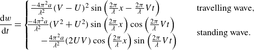 \begin{align} { \frac {\textrm {d} w}{\textrm {d}t} = \begin{cases} \frac {-4 \pi ^2 a}{\lambda ^2} (V- U)^2 \sin \left (\frac {2 \pi }{\lambda } x- \frac {2 \pi }{\lambda } Vt\right ) & \quad \text {travelling wave},\\ {\begin{array}{l}\!\!\!\frac {-4 \pi ^2 a}{\lambda ^2} (V^2+U^2) \sin \left ( \frac {2\pi }{\lambda }x\right )\cos \left (\frac {2 \pi }{\lambda } Vt \right ) \\ \quad-\frac {4 \pi ^2 a}{\lambda ^2} (2UV)\cos \left ( \frac {2\pi }{\lambda }x\right )\sin \left (\frac {2 \pi }{\lambda } Vt \right )\end{array}} & \quad \text {standing wave}. \\ \end{cases}} \end{align}
Equation (B3) clearly shows that the amplitude of lateral fluid acceleration $\textrm {d} w/\textrm {d}t$
decreases as swimming speed
$\textrm {d} w/\textrm {d}t$
decreases as swimming speed $U$
increases in the travelling wave, whereas for the standing wave lateral acceleration increases with swimming speed, monotonically. This amplitude when reaching the maximum value of swimming speed is much higher for the standing wave kinematics. This is why when swimmers reach the steady swimming speed, the pressure on the body surface is higher on the lamprey with the standing wave kinematics compared with the one with the travelling wave (see figures 8 and 9). This is true for undulations with arbitrary coefficient
$U$
increases in the travelling wave, whereas for the standing wave lateral acceleration increases with swimming speed, monotonically. This amplitude when reaching the maximum value of swimming speed is much higher for the standing wave kinematics. This is why when swimmers reach the steady swimming speed, the pressure on the body surface is higher on the lamprey with the standing wave kinematics compared with the one with the travelling wave (see figures 8 and 9). This is true for undulations with arbitrary coefficient $a(x)$
.
$a(x)$
.
Lighthill (Reference Lighthill1960) also used elongated body theory to obtain the thrust of an undulatory swimmer as
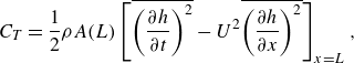 \begin{align} C_T=\frac {1}{2} \rho A(L) \left [ \overline {\left (\frac {\partial h}{\partial t}\right )^2} - U^2 \overline {\left (\frac {\partial h}{\partial x}\right )^2} \right ]_{x=L} , \end{align}
where $\overline {()}$
denotes average and
$\overline {()}$
denotes average and $\rho A(L)$
is the virtual (added) mass of the cross-section at the tail and the cross-section mass at the anterior is assumed to be zero. Substituting both kinematics of (B1) into this equation the thrust force is calculated as
$\rho A(L)$
is the virtual (added) mass of the cross-section at the tail and the cross-section mass at the anterior is assumed to be zero. Substituting both kinematics of (B1) into this equation the thrust force is calculated as
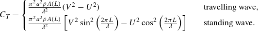 \begin{align} C_T = \begin{cases} \frac {\pi ^2 a^2 \rho A(L)}{\lambda ^2} (V^2- U^2) & \quad \text {travelling wave},\\[3pt] \frac {\pi ^2 a^2 \rho A(L)}{\lambda ^2} \left [ V^2 \sin ^2\left (\frac {2\pi L}{\lambda }\right ) -U^2 \cos ^2\left (\frac {2\pi L}{\lambda }\right )\right ] & \quad \text {standing wave}. \\ \end{cases} \end{align}
For both kinematics the wavelength is $\lambda =0.65 L$
for the lamprey, which is in agreement with experimental observations of lampreys in nature (Hultmark et al. Reference Hultmark, Leftwich and Smits2007). Based on the above equation and corresponding values for wavelength, the travelling wave produces a significantly higher thrust force than the standing wave (see figure 5) and the thrust force monotonically decreases as the swimming speed increases for both kinematics.
$\lambda =0.65 L$
for the lamprey, which is in agreement with experimental observations of lampreys in nature (Hultmark et al. Reference Hultmark, Leftwich and Smits2007). Based on the above equation and corresponding values for wavelength, the travelling wave produces a significantly higher thrust force than the standing wave (see figure 5) and the thrust force monotonically decreases as the swimming speed increases for both kinematics.
Finally, the mean rate of work (time-averaged power consumption) by swimmers can be calculated through the same theory as
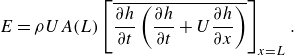 \begin{align} E = \rho U A(L) \left [ \overline { \frac {\partial h}{\partial t} \left (\frac {\partial h}{\partial t} + U \frac {\partial h}{\partial x}\right )} \right ]_{x=L} . \end{align}
This value for travelling and standing wave kinematics is computed as follows:
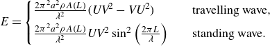 \begin{align} E = \begin{cases} \frac {2 \pi ^2 a^2 \rho A(L)}{\lambda ^2} (\textit{UV}^2- \textit{VU}^2) & \quad \text {travelling wave},\\[4pt] \frac {2 \pi ^2 a^2 \rho A(L)}{\lambda ^2} \textit{UV}^2 \sin ^2\left (\frac {2\pi L}{\lambda } \right ) & \quad \text {standing wave}. \\ \end{cases} \end{align}


 Open access