


1. Introduction
Pressure-driven flows of viscoelastic polymer solutions in narrow non-uniform geometries are widely encountered in industrial processes, such as extrusion (Pearson Reference Pearson1985; Tadmor & Gogos Reference Tadmor and Gogos2013), and in various applications ranging from microfluidic extensional rheometers (Ober et al. Reference Ober, Haward, Pipe, Soulages and McKinley2013) to devices for subcutaneous drug administration, in which the liquid may exhibit non-Newtonian behaviour (Allmendinger et al. Reference Allmendinger, Fischer, Huwyler, Mahler, Schwarb, Zarraga and Mueller2014; Fischer et al. Reference Fischer, Schmidt, Bryant and Besheer2015). The complex rheological behaviour of viscoelastic fluids affects the hydrodynamic features of such flows, including the relationship between the pressure drop  $\Delta p$ across the channel and the flow rate $q$ even at low Reynolds number.
The dependence of the pressure drop on the flow rate of viscoelastic fluids at low Reynolds number has been studied extensively in various geometries. Table 1 lists a chronological selection of previous work on the  $q$–
$q$– $\Delta p$ relation for viscoelastic fluids in non-uniform geometries and clearly illustrates that the vast majority of the previous work involved numerical simulations and experimental measurements.
Table 1. Chronological selection of previous experimental, numerical and theoretical papers on the flow rate–pressure drop relation for the low-Reynolds-number flows of viscoelastic fluids in non-uniform geometries.

The early studies on the flow rate–pressure drop relation have mainly investigated abrupt geometries such as contraction and contraction–expansion channels. For such geometries, the two-dimensional (2-D) and axisymmetric numerical simulations with constitutive models, such as the Oldroyd-B model and finite-extensibility nonlinear elastic (FENE-CR) model introduced by Chilcott & Rallison (Reference Chilcott and Rallison1988), have generally predicted a reduction in the pressure drop with increasing Weissenberg ( $Wi$) or Deborah ( $De$) numbers, which are defined in § 2.1 (Keiller Reference Keiller1993; Szabo et al. Reference Szabo, Rallison and Hinch1997; Aboubacar et al. Reference Aboubacar, Matallah and Webster2002; Alves et al. Reference Alves, Oliveira and Pinho2003; Binding et al. Reference Binding, Phillips and Phillips2006; Oliveira et al. Reference Oliveira, Oliveira, Pinho and Alves2007; Aguayo et al. Reference Aguayo, Tamaddon-Jahromi and Webster2008; Tamaddon-Jahromi et al. Reference Tamaddon-Jahromi, Webster and Walters2010, Reference Tamaddon-Jahromi, Webster and Williams2011). The exceptions are simulations with small values of the finite extensibility parameter in the FENE-CR model that have reported an initial decrease in the pressure drop followed by a slight increase of the order of 10 $\%$ (Szabo et al. Reference Szabo, Rallison and Hinch1997; Tamaddon-Jahromi et al. Reference Tamaddon-Jahromi, Webster and Walters2010, Reference Tamaddon-Jahromi, Webster and Williams2011). However, these predictions are in contrast with the experimental results of Rothstein & McKinley (Reference Rothstein and McKinley1999, Reference Rothstein and McKinley2001), Nigen & Walters (Reference Nigen and Walters2002) and Sousa et al. (Reference Sousa, Coelho, Oliveira and Alves2009) for the flow of a polymer solution (Boger fluid) through abrupt axisymmetric contraction–expansion and contraction geometries that have reported a nonlinear increase in the pressure drop with the flow rate. Such an increase in the pressure drop was observed also in experimental studies on microfluidic rectifiers, which further showed the dependence of the flow rate–pressure drop relation on the flow direction (Groisman & Quake Reference Groisman and Quake2004; Nguyen et al. Reference Nguyen, Lam, Ho and Low2008; Sousa et al. Reference Sousa, Pinho, Oliveira and Alves2010).
It is widely hypothesised that this discrepancy is attributed to the inability of the continuum macroscale constitutive models, such as Oldroyd-B, FENE-CR and the finite-extensibility nonlinear elastic model with the Peterlin approximation (FENE-P), to describe accurately the microscopic features of the polymer solutions (Owens & Phillips Reference Owens and Phillips2002; Afonso et al. Reference Afonso, Oliveira, Pinho and Alves2011). As shown by Koppol et al. (Reference Koppol, Sureshkumar, Abedijaberi and Khomami2009), a mesoscopic level, micromechanical description, such as the bead–rod and bead–spring models, can be used to resolve, at least partially, this contradiction. For example, using the mesoscopic bead–spring chain model, Koppol et al. (Reference Koppol, Sureshkumar, Abedijaberi and Khomami2009) showed an increase in the pressure drop for viscoelastic flow in an axisymmetric contraction–expansion geometry, which is in qualitative agreement with the experiments of Rothstein & McKinley (Reference Rothstein and McKinley1999). However, Koppol et al. (Reference Koppol, Sureshkumar, Abedijaberi and Khomami2009) were not able to observe such an agreement for simulations with the continuum FENE-P model, thus indicating the advantage of mesoscopic over macroscopic simulations.
Nevertheless, it should be noted that, to date, the mesoscopic simulations are still computationally expensive and difficult to perform in complex geometries, requiring refined meshing and time-stepping for accurate viscoelastic predictions (Keunings Reference Keunings2004; Afonso et al. Reference Afonso, Oliveira, Pinho and Alves2011; Alves, Oliveira & Pinho Reference Alves, Oliveira and Pinho2021). Therefore, despite the limitations of a continuum approach, the vast majority of studies in non-Newtonian fluid mechanics still exploit the macroscopic constitutive equations, such as Oldroyd-B, FENE-CR and FENE-P, which, in principle, can be modified to incorporate some microscopic features. For instance, Webster and co-workers proposed a new constitutive equation, which is the hybrid combination of White and Metzner (White & Metzner Reference White and Metzner1963) and FENE-CR models (WM-FENE-CR; see, e.g., Tamaddon-Jahromi et al. Reference Tamaddon-Jahromi, Webster and Williams2011, Reference Tamaddon-Jahromi, Garduño, López-Aguilar and Webster2016; Webster et al. Reference Webster, Tamaddon-Jahromi, López-Aguilar and Binding2019). Specifically, in this model, the deviatoric stress tensor  $\boldsymbol {\tau }$, which is the sum of the Newtonian solvent and viscoelastic polymer contributions, is obtained by multiplying the expression for $\boldsymbol {\tau }$ from the FENE-CR model by a dissipative function $\phi (\dot {\varepsilon })$, usually taken as $\phi (\dot {\varepsilon })=1+(\lambda _{D}\dot {\varepsilon })^{2}$, where $\lambda _{D}$ is an additional time constant and $\dot {\varepsilon }=3\boldsymbol {III}_{\boldsymbol {E}}/\boldsymbol {II}_{\boldsymbol {E}}$ is the generalised extension rate based on the second and third invariants of the rate-of-strain tensor $\boldsymbol{\mathsf{E}}$ defined in § 2.1, wherein $\boldsymbol {II}_{{E}}=\mbox {tr}(\boldsymbol{\mathsf{E}}^{2})/2$ and $\boldsymbol {III}_{{E}}=\mbox {det}(\boldsymbol{\mathsf{E}})$ (Tamaddon-Jahromi et al. Reference Tamaddon-Jahromi, Garduño, López-Aguilar and Webster2016). Such a model exhibits a constant shear viscosity, finite extensibility with a bounded extensional viscosity that reaches an ultimate plateau, and a first-normal stress-difference that has a weaker than quadratic dependence on the shear rate in the Oldroyd-B model. Using this hybrid WM-FENE-CR model, Webster and co-workers were able to achieve quantitative agreement between their numerical predictions for the pressure drop and the earlier experiments of Rothstein & McKinley (Reference Rothstein and McKinley2001) and Nigen & Walters (Reference Nigen and Walters2002), where $\lambda _{D}$ and finite extensibility served as fitting parameters (López-Aguilar et al. Reference López-Aguilar, Tamaddon-Jahromi, Webster and Walters2016; Tamaddon-Jahromi et al. Reference Tamaddon-Jahromi, Garduño, López-Aguilar and Webster2016, Reference Tamaddon-Jahromi, López-Aguilar and Webster2018).
After primarily focusing on abrupt contractions or contraction–expansions geometries a decade ago, hyperbolic symmetric channels with nearly constant extensional rates along the centreline have also received much attention, and several groups suggested to use of hyperbolic geometries for obtaining extensional properties of viscoelastic fluids through  $q$–
$q$– $\Delta p$ measurements (Campo-Deaño et al. Reference Campo-Deaño, Galindo-Rosales, Pinho, Alves and Oliveira2011; Nyström et al. Reference Nyström, Tamaddon-Jahromi, Stading and Webster2012, Reference Nyström, Tamaddon-Jahromi, Stading and Webster2016, Reference Nyström, Tamaddon-Jahromi, Stading and Webster2017; Ober et al. Reference Ober, Haward, Pipe, Soulages and McKinley2013; Keshavarz & McKinley Reference Keshavarz and McKinley2016; Zografos et al. Reference Zografos, Hartt, Hamersky, Oliveira, Alves and Poole2020). However, recently some researchers conjectured that, given the complex mixture of shear and extensional flow components in this geometry, it is difficult to determine extensional viscosity directly from $q$–
$q$– $\Delta p$ data (James Reference James2016; Hsiao et al. Reference Hsiao, Dinic, Ren, Sharma and Schroeder2017).
Of particular interest is a recent experimental study of James & Roos (Reference James and Roos2021) on the pressure-driven flow of Boger fluids through a long hyperbolic contracting channel. James & Roos (Reference James and Roos2021) measured the pressure drop for various flow rates and found that the pressure drop matches equivalent Newtonian measurements, in contrast to previous experimental results showing a nonlinear increase in the pressure drop with the flow rate (see, e.g., Rothstein & McKinley Reference Rothstein and McKinley1999, Reference Rothstein and McKinley2001; Campo-Deaño et al. Reference Campo-Deaño, Galindo-Rosales, Pinho, Alves and Oliveira2011; Ober et al. Reference Ober, Haward, Pipe, Soulages and McKinley2013). The explanation for this discrepancy lies in the different pressure drops measured by the different sets of authors. The experimental set-up of James & Roos (Reference James and Roos2021) consisted of a hyperbolic contracting channel connected upstream to a long straight channel. The fluid was driven by pressurised air to flow through a straight section, entered the contracting channel and then exited to the atmosphere. James & Roos (Reference James and Roos2021) defined the pressure drop as the difference between the air pressure required to drive the fluid through a straight section and the atmospheric pressure at the end of the channel, where die swell occurred.
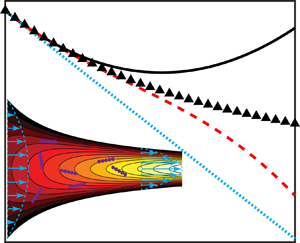
In contrast to pressure drop measurements of James & Roos (Reference James and Roos2021) that included the apparent exit effects, most of the previous experimental studies eliminated the entrance and exit effects (see, e.g., Rothstein & McKinley Reference Rothstein and McKinley1999, Reference Rothstein and McKinley2001; Campo-Deaño et al. Reference Campo-Deaño, Galindo-Rosales, Pinho, Alves and Oliveira2011; Ober et al. Reference Ober, Haward, Pipe, Soulages and McKinley2013). For example, the experimental set-up of Rothstein & McKinley (Reference Rothstein and McKinley1999) consisted of two long straight channels connected to the non-uniform region upstream and downstream, and the pressure drop was measured in these straight channels far from the entrance and exit. In this work, we follow the study of Rothstein & McKinley (Reference Rothstein and McKinley1999) and explore the pressure drop originating from the non-uniformity of geometry while eliminating the entrance and exit effects (see figure 1).

Figure 1. Schematic illustration of the 2-D configuration consisting of a slowly spatially varying and symmetric channel of height  $2h(z)$ and length $\ell$ ( $h\ll \ell$), connected to two long straight channels of height $2h_{0}$ and $2h_{\ell }$, respectively. The configuration contains a viscoelastic dilute polymer solution steadily driven by the imposed flow rate $q$. We are interested in determining the pressure drop $\Delta p$ over a streamwise distance $\ell$, arising from the non-uniformity of geometry, while eliminating the entrance and exit effects.
It should be noted that, in addition to abrupt contracting and hyperbolic channels, the flow rate–pressure drop relation of viscoelastic fluids has been studied in other geometries, such as converging (Black & Denn Reference Black and Denn1976) and undulating (Pilitsis & Beris Reference Pilitsis and Beris1989; Souvaliotis & Beris Reference Souvaliotis and Beris1992) channels. For example, Black & Denn (Reference Black and Denn1976) studied the pressure-driven flow of the upper-convected Maxwell (UCM) fluid in a rectilinearly converging channel. Applying the sink flow approximation and assuming a weakly viscoelastic limit, Black & Denn (Reference Black and Denn1976) provided a perturbation solution to the flow field up to second order in Weissenberg number. Black & Denn (Reference Black and Denn1976) also depicted the first three terms of a perturbation solution for the power required to drive the fluid as a function of  $Wi$, indicating that the first viscoelastic correction decreases the power or pressure drop. However, no explicit expressions nor validation of this result by comparison with simulations has been presented. In addition, Pilitsis & Beris (Reference Pilitsis and Beris1989) studied numerically the pressure-driven flow of the UCM and Oldroyd-B fluids in an undulating cylinder and showed a small reduction in the hydrodynamic resistance, defined as a ratio of the pressure drop to the flow rate, with increasing Weissenberg number.
Recently, Pérez-Salas et al. (Reference Pérez-Salas, Sánchez, Ascanio and Aguayo2019) studied analytically and numerically the pressure-driven flow of a Phan-Thien–Tanner (PTT) fluid (Phan-Thien & Tanner Reference Phan-Thien and Tanner1977; Phan-Thien Reference Phan-Thien1978) through a planar hyperbolic contraction. Using lubrication theory and neglecting the solvent contribution, Pérez-Salas et al. (Reference Pérez-Salas, Sánchez, Ascanio and Aguayo2019) derived closed-form expressions for the non-dimensional velocity and pressure fields, which depend on the channel geometry and the product  $\varepsilon _{PTT}Wi^2$, where $\varepsilon _{PTT}$ is the extensibility parameter of the PTT model. Their results predicted a decrease in the pressure drop with increasing $Wi$. However, such a reduction in the pressure drop arises due to shear-thinning effects of the PTT fluid, which are manifested when $Wi$ increases. Moreover, for $\varepsilon _{PTT}=0$, corresponding to the Oldroyd-B model, the solution of Pérez-Salas et al. (Reference Pérez-Salas, Sánchez, Ascanio and Aguayo2019) reduces to the Newtonian solution, which is independent of $Wi$.
$Wi$.
In the context of lubrication theory, it is worth mentioning earlier studies on the pressure-driven flow of a fibre suspension in a slowly varying channel, which showed the ability of the lubrication approach to capture well the flow field (Rallison & Keiller Reference Rallison and Keiller1993; Sykes & Rallison Reference Sykes and Rallison1997). We have recently exploited the Lorentz reciprocal theorem and lubrication theory to derive a closed-form expression for the flow rate–pressure drop relation for complex fluids in narrow geometries, which holds for a wide class of non-Newtonian constitutive models (Boyko & Stone Reference Boyko and Stone2021). We showed the use of our theory to calculate analytically the first-order non-Newtonian correction for the  $q$–
$q$– $\Delta p$ relation for the viscoelastic second-order fluid and shear-thinning Carreau fluid, solely using the corresponding Newtonian solution and bypassing solution of the non-Newtonian flow problem.
To the best of the authors’ knowledge, no analytical solution for the  $q$–
$q$– $\Delta p$ relation for constant shear-viscosity viscoelastic (Boger) fluids in narrow geometries has been reported in the literature, even for ‘simple’ models such as Oldroyd-B and FENE-CR in the weakly viscoelastic limit. Such analytical solutions, however, are of fundamental importance as they may be used directly for comparison with experimental data and, in the case of discrepancy between the theory and experiments, may provide insight into the cause of this disagreement and the adequacy of the constitutive model.
In this work, we provide a theoretical framework for calculating the flow rate–pressure drop relation of viscoelastic fluids in narrow channels of slowly varying arbitrary shapes. The present work presents analytical results for velocity and pressure fields and the  $q$–
$q$– $\Delta p$ relation for the Oldroyd-B model in the weakly viscoelastic limit. In subsequent work, we will analyse more complex constitutive models, incorporating additional microscopic features of polymer solutions. Our approach for obtaining analytical solutions for velocity and pressure is motivated by studies on thin films and lubrication problems (Tichy Reference Tichy1996; Zhang, Matar & Craster Reference Zhang, Matar and Craster2002; Saprykin, Koopmans & Kalliadasis Reference Saprykin, Koopmans and Kalliadasis2007; Ahmed & Biancofiore Reference Ahmed and Biancofiore2021). Such an approach relies on exploiting the narrowness of the geometry through the application of the lubrication approximation and a perturbation expansion in powers of the Deborah number $De$, which is assumed to be small, $De\ll 1$, and solving order by order, often resulting in cumbersome calculations at high orders. Instead, once the velocity at $O(De^2)$ is obtained, we use the reciprocal theorem, recently derived by Boyko & Stone (Reference Boyko and Stone2021), to calculate the pressure drop at $O(De^3)$, bypassing the detailed calculations of the viscoelastic flow problem at this order and relying only on the solution from previous orders. To validate the analytical results of our model, we perform 2-D finite-element numerical simulations with the Oldroyd-B model and find a good agreement between the theory and simulations, even for the cases when the hypotheses behind the lubrication approximation are not strictly satisfied. Given the recognised shortcomings of the Oldroyd-B and commonly used continuum finite-extensibility nonlinear elastic (FENE) models in predicting the experimental observations for the flow rate–pressure drop relation, we are hopeful that the insights presented here may be useful in understanding possible physical or molecularly inspired modifications to the constitutive descriptions to improve future modeling and simulation efforts.
The paper is organised as follows. In § 2, we present the problem formulation and the dimensional governing equations and boundary conditions for the pressure-driven flow of the Oldroyd-B fluid. We further identify the characteristic scales and dimensionless parameters governing the flow and provide the non-dimensional governing equations. In § 3, we present a low-Deborah-number lubrication analysis and derive closed-form analytical solutions for the flow field and pressure drop up to  $O(De^2)$. Exploiting the reciprocal theorem, in § 4 we calculate the pressure drop at $O(De^3)$, relying only on the solutions from previous orders. We present the results in § 5, including a comparison between the analytical predictions and the 2-D numerical simulations, finding excellent agreement between the two approaches. We conclude with a discussion of the results in § 6.
2. Problem formulation and governing equations
We study the incompressible steady flow of a non-Newtonian viscoelastic dilute polymer solution in a slowly spatially varying and symmetric 2-D channel of height  $2h(z)$ and length $\ell$, where $h\ll \ell$. We assume that the imposed flow rate $q$ (per unit depth) induces the fluid motion with pressure distribution $p$ and velocity $\boldsymbol {u}=(u_{z},u_{y})$. Our primary interest is to determine, for a non-uniform geometry, the pressure drop $\Delta p$ over a streamwise distance $\ell$, while eliminating the entrance and exit effects. To this end, motivated by the geometries used in previous experimental and numerical studies (see, e.g., Szabo et al. Reference Szabo, Rallison and Hinch1997; Rothstein & McKinley Reference Rothstein and McKinley1999; Alves et al. Reference Alves, Oliveira and Pinho2003; Alves & Poole Reference Alves and Poole2007; Campo-Deaño et al. Reference Campo-Deaño, Galindo-Rosales, Pinho, Alves and Oliveira2011; Ober et al. Reference Ober, Haward, Pipe, Soulages and McKinley2013; Zografos et al. Reference Zografos, Hartt, Hamersky, Oliveira, Alves and Poole2020; Zargartalebi, Zargartalebi & Benneker Reference Zargartalebi, Zargartalebi and Benneker2021), we assume that the inlet ( $z=0$) and outlet ( $z=\ell$) of the non-uniform region are connected to two long straight channels of height $2h_{0}$ and $2h_{\ell }$, and length $\ell _{en}$ and $\ell _{ex}$, respectively. Consequently, the flow is fully developed at the inlet of the non-uniform region and becomes fully developed again towards the exit of the configuration. Figure 1 presents a schematic illustration of the 2-D configuration and the coordinate system $(y,z)$, whose $z$ axes lies in the symmetry midplane of the channel and $y$ is in the direction of the shortest dimension. It should be noted that when a viscoelastic fluid exits from the non-uniform region directly to the atmosphere or a large reservoir, there can be significant exit effects due to axial stresses (James & Roos Reference James and Roos2021).
While throughout this work we consider steady and stable flows, it should be noted that the flow of viscoelastic fluids within non-uniform geometries may become unstable above a certain flow rate even at low Reynolds numbers due to the fluid's complex rheology (Larson Reference Larson1992; Shaqfeh Reference Shaqfeh1996; Datta et al. Reference Datta2021; Steinberg Reference Steinberg2021). We consider low-Reynolds-number flows, so that the fluid inertia is negligible relative to viscous stresses. In this limit, the fluid motion is governed by the continuity and momentum equations
 \begin{equation} \boldsymbol{\nabla\cdot u}=0,\quad\boldsymbol{\nabla\cdot\sigma}=\boldsymbol{0},\end{equation}
where  $\boldsymbol {\sigma }$ is the stress tensor given by
 \begin{equation} \boldsymbol{\sigma}={-}p\boldsymbol{\mathsf{I}}+2\eta_{s}\boldsymbol{\mathsf{E}}+\boldsymbol{\tau}_{p}.\end{equation}
The first term on the right-hand side of (2.2) is the pressure contribution, the second term is the viscous stress contribution of Newtonian solvent with a constant viscosity  $\eta _{s}$, where $\boldsymbol{\mathsf{E}}=(\boldsymbol {\nabla }\boldsymbol {u} +(\boldsymbol {\nabla }\boldsymbol {u})^{\mathrm {T}})/2$ is the rate-of-strain tensor, and the last term, $\boldsymbol {\tau }_{p}$, is the polymer contribution to the stress tensor.
In this work, we describe the viscoelastic behaviour of the polymer solution using the Oldroyd-B constitutive model (Bird, Armstrong & Hassager Reference Bird, Armstrong and Hassager1987). This is a widely used continuum model for Boger fluids, characterised by a constant shear viscosity. The Oldroyd-B equation can be derived from microscopic principles by modeling the polymer molecules as dumbbells, which follow a linear Hooke's law for the restoring force as they are advected and stretched by the flow. In the Oldroyd-B model, the polymer contribution to the stress tensor  $\boldsymbol {\tau }_{p}$ can be expressed in the form (Bird et al. Reference Bird, Armstrong and Hassager1987; Morozov & Spagnolie Reference Morozov and Spagnolie2015; Alves et al. Reference Alves, Oliveira and Pinho2021)
 \begin{equation} \boldsymbol{\tau}_{p}=\frac{\eta_{p}}{\lambda} (\boldsymbol{\mathsf{A}}-\boldsymbol{\mathsf{I}}),\end{equation}
where  $\eta _{p}$ is the polymer contribution to the shear viscosity at zero shear rate and $\lambda$ is the longest relaxation time of the polymers. In (2.3), $\boldsymbol{\mathsf{A}}$ is the conformation tensor of the dumbbells, which denotes the ensemble average of the second moment of the dumbbell end-to-end vector $\boldsymbol {r}$ (scaled with its equilibrium value), $\boldsymbol{\mathsf{A}}\equiv \langle \boldsymbol {rr}\rangle$, and evolves at steady state according to (Bird et al. Reference Bird, Armstrong and Hassager1987; Morozov & Spagnolie Reference Morozov and Spagnolie2015; Alves et al. Reference Alves, Oliveira and Pinho2021)
 \begin{equation} \boldsymbol{u}\boldsymbol{\cdot}\boldsymbol{\nabla}\boldsymbol{\mathsf{A}}- (\boldsymbol{\nabla}\boldsymbol{u})^{\mathrm{T}}\boldsymbol{\cdot} \boldsymbol{\mathsf{A}}-\boldsymbol{\mathsf{A}}\boldsymbol{\cdot}(\boldsymbol{\nabla} \boldsymbol{u})={-}\frac{1}{\lambda}(\boldsymbol{\mathsf{A}}-\boldsymbol{\mathsf{I}}).\end{equation}
Combining (2.3) and (2.4), we obtain an evolution equation for the polymer contribution to the stress tensor  $\boldsymbol {\tau }_{p}$, given at steady state as (Bird et al. Reference Bird, Armstrong and Hassager1987; Morozov & Spagnolie Reference Morozov and Spagnolie2015; Alves et al. Reference Alves, Oliveira and Pinho2021),
 \begin{equation} \boldsymbol{\tau}_{p}+\lambda[\boldsymbol{u}\boldsymbol{\cdot} \boldsymbol{\nabla}\boldsymbol{\tau}_{p}-(\boldsymbol{\nabla} \boldsymbol{u})^{\mathrm{T}}\boldsymbol{\cdot}\boldsymbol{\tau}_{p}- \boldsymbol{\tau}_{p}\boldsymbol{\cdot}(\boldsymbol{\nabla}\boldsymbol{u})]= 2\eta_{p}\boldsymbol{\mathsf{E}}.\end{equation}
Using (2.2), (2.3) and (2.5), the stress tensor  $\boldsymbol {\sigma }$ can be also expressed as
 \begin{equation} \boldsymbol{\sigma}={-}p\boldsymbol{\mathsf{I}}+2\eta_{0}\boldsymbol{\mathsf{E}}+ \eta_{p}\boldsymbol{\mathsf{S}},\end{equation}
where  $\eta _{0}=\eta _{s}+\eta _{p}$ is the total zero-shear-rate viscosity of the polymer solution and $\boldsymbol {S}$ is defined through $\boldsymbol {\tau }_{p}=2\eta _{p}\boldsymbol{\mathsf{E}}+\eta _{p}\boldsymbol{\mathsf{S}}$, so that
 \begin{align} \boldsymbol{\mathsf{S}}&={-}\frac{\lambda}{\eta_{p}}[\boldsymbol{u} \boldsymbol{\cdot}\boldsymbol{\nabla}\boldsymbol{\tau}_{p}- (\boldsymbol{\nabla}\boldsymbol{u})^{\mathrm{T}}\boldsymbol{ \cdot}\boldsymbol{\tau}_{p}-\boldsymbol{\tau}_{p}\boldsymbol{\cdot} (\boldsymbol{\nabla}\boldsymbol{u})]\nonumber\\ &={-}[\boldsymbol{u}\boldsymbol{\cdot}\boldsymbol{\nabla}\boldsymbol{\mathsf{A}}- (\boldsymbol{\nabla}\boldsymbol{u})^{\mathrm{T}}\boldsymbol{\cdot}(\boldsymbol{\mathsf{A}}- \boldsymbol{\mathsf{I}})-(\boldsymbol{\mathsf{A}}-\boldsymbol{\mathsf{I}})\boldsymbol{\cdot} (\boldsymbol{\nabla}\boldsymbol{u})]. \end{align}
Substituting (2.6) into (2.1) provides an alternative form of the governing equations
 \begin{equation} \boldsymbol{\nabla\cdot u}=0,\quad\boldsymbol{\nabla}p=\eta_{0}\nabla^2\boldsymbol{u} + \eta_{p}\boldsymbol{\nabla\cdot \boldsymbol{\mathsf{S}}},\end{equation}
which is convenient for assessing the viscoelastic effects on the flow and pressure fields, where  $\boldsymbol{\mathsf{S}}$ is given in (2.7) and $\boldsymbol{\mathsf{A}}$ evolves according to (2.4).
The governing equations (2.1)–(2.8) are supplemented by the boundary conditions
 $$\begin{gather} u_{z}(h(z),z)=0,\quad u_{y}(h(z),z)=0,\quad\frac{\partial u_{z}}{\partial y}(0,z)=0, \end{gather}$$
 $$\begin{gather}u_{z}(y,-\ell_{en})=\frac{3q}{4}\frac{h_{0}^{2}-y^{2}}{h_{0}^{3}},\quad u_{z}(y,\ell+\ell_{ex})=\frac{3q}{4} \frac{h_{\ell}^{2}-y^{2}}{h_{\ell}^{3}}, \end{gather}$$
 $$\begin{gather}A_{zz}(y,-\ell_{en})=1+\frac{9}{2}\left(\frac{\lambda qy}{h_{0}^{3}}\right)^{2},\quad A_{yz}(y,-\ell_{en})={-}\frac{3\lambda qy}{2h_{0}^{3}},\quad A_{yy}(y,-\ell_{en})=1. \end{gather}$$
The first three boundary conditions (2.9a–c) correspond to the no-slip and no-penetration boundary conditions along the channel walls and the symmetry boundary condition at the centreline, respectively. Equations (2.9d,e) correspond to the fully developed unidirectional Poiseuille velocity profile at the entrance and exit. These two boundary conditions ensure that the integral constraint  $2\int _{0}^{h(z)}u_{z}(y,z)\,\mathrm {d} y=q$ is satisfied along the channel. In addition, at the entrance, we impose the polymer stress (or conformation tensor) distribution corresponding to the Poiseuille flow, as given in (2.9a–c) to (2.9f–h) (Szabo et al. Reference Szabo, Rallison and Hinch1997; Koppol et al. Reference Koppol, Sureshkumar, Abedijaberi and Khomami2009). In addition, at the exit, the reference value for the pressure is set to zero on $y=0$.
2.1. Scaling analysis and non-dimensionalisation
In this work, we examine narrow configurations, in which  $h(z)\ll \ell$, $h_{\ell }$ is the half-height at $z=\ell$ and $u_{c}=q/2h_{\ell }$ is the characteristic velocity scale set by the cross-sectionally averaged velocity. Note that for the 2-D case, the flow rate $q$ is per unit depth.
We introduce non-dimensional variables based on lubrication theory (Tichy Reference Tichy1996; Zhang et al. Reference Zhang, Matar and Craster2002; Saprykin et al. Reference Saprykin, Koopmans and Kalliadasis2007; Ahmed & Biancofiore Reference Ahmed and Biancofiore2021),
 $$\begin{gather} Z=\frac{z}{\ell},\quad Y=\frac{y}{h_{\ell}}, \quad U_{z}=\frac{u_{z}}{u_{c}},\quad U_{y}=\frac{u_{y}}{\epsilon u_{c}}, \end{gather}$$
 $$\begin{gather}P=\frac{p}{\eta_{0}u_{c}\ell/h_{\ell}^{2}},\quad\Delta P=\frac{\Delta p}{\eta_{0}u_{c}\ell/h_{\ell}^{2}},\quad H=\frac{h}{h_{\ell}}, \end{gather}$$
 $$\begin{gather}\mathcal{T}_{p,zz}=\frac{\epsilon^{2}\ell}{\eta_{0}u_{c}}\tau_{p,zz},\quad \tilde{A}_{zz}=\frac{\epsilon^{2}(A_{zz}-1)}{De},\quad \mathcal{S}_{zz}=\frac{\epsilon^{2}\ell}{u_{c}De} S_{zz}, \end{gather}$$
 $$\begin{gather}\mathcal{T}_{p,yz}=\frac{\epsilon\ell}{\eta_{0}u_{c}}\tau_{p,yz},\quad \tilde{A}_{yz}=\frac{\epsilon A_{yz}}{De},\quad \mathcal{S}_{yz}=\frac{\epsilon \ell}{u_{c} De}S_{yz}, \end{gather}$$
 $$\begin{gather}\mathcal{T}_{p,yy}=\frac{\ell}{\eta_{0}u_{c}}\tau_{p,yy},\quad \tilde{A}_{yy}=\frac{A_{yy}-1}{De}, \quad \mathcal{S}_{yy}= \frac{\ell}{u_{c} De}S_{yy}, \end{gather}$$
where we have introduced the aspect ratio of the configuration, which is assumed to be small,
 \begin{equation} \epsilon=\frac{h_{\ell}}{\ell}\ll1,\end{equation}
the viscosity ratios,
 \begin{equation} \tilde{\beta}=\frac{\eta_{p}}{\eta_{s}+\eta_{p}}=\frac{\eta_{p}}{\eta_{0}}\quad\mbox{and}\quad \beta=1-\tilde{\beta}=\frac{\eta_{s}}{\eta_{0}}, \end{equation}
and the Deborah and Weissenberg numbers,
 \begin{equation} De=\frac{\lambda u_{c}}{\ell}\quad\mbox{and}\quad Wi=\frac{\lambda u_{c}}{h_{\ell}}.\end{equation}
The non-dimensional shape of the channel is denoted by  $H(Z)$ and is an important parameter in our analysis.
Following Ahmed & Biancofiore (Reference Ahmed and Biancofiore2021), we define the Deborah number  $De$ as the ratio of the polymer relaxation time, $\lambda$, to the residence time in the spatially non-uniform region, $\ell /u_{c}$, or alternatively, as the product of the relaxation time scale of the fluid and the characteristic extensional rate of the flow (see also Tichy Reference Tichy1996; Zhang et al. Reference Zhang, Matar and Craster2002; Saprykin et al. Reference Saprykin, Koopmans and Kalliadasis2007). The Weissenberg number $Wi$ is the product of the relaxation time scale of the fluid and the characteristic shear rate of the flow, and is related to the Deborah number through $De=\epsilon Wi$ (Ahmed & Biancofiore Reference Ahmed and Biancofiore2021). We note that since we assume $\epsilon \ll 1$, $De$ can be small while keeping $Wi =O(1)$.
2.2. Governing equations in dimensionless form
Using the non-dimensionalisation (2.10)–(2.13), the governing equations (2.1)–(2.9) take the form
 $$\begin{gather} \frac{\partial U_{z}}{\partial Z}+ \frac{\partial U_{y}}{\partial Y}=0, \end{gather}$$
 $$\begin{gather}\frac{\partial P}{\partial Z}=\epsilon^{2} \frac{\partial^{2}U_{z}}{\partial Z^{2}}+\frac{\partial^{2}U_{z}}{\partial Y^{2}} +\tilde{\beta} De\frac{\partial \mathcal{S}_{zz}}{\partial Z}+\tilde{\beta} De\frac{\partial \mathcal{S}_{yz}}{\partial Y}, \end{gather}$$
 $$\begin{gather}\frac{\partial P}{\partial Y}=\epsilon^{4}\frac{\partial^{2}U_{y}}{\partial Z^{2}}+\epsilon^{2}\frac{\partial^{2}U_{y}}{\partial Y^{2}}+\epsilon^{2}\tilde{\beta}De \frac{\partial \mathcal{S}_{yz}}{\partial Z}+\epsilon^{2}\tilde{\beta} De\frac{\partial \mathcal{S}_{yy}}{\partial Y}, \end{gather}$$
 $$\begin{gather}De\left(U_{z}\frac{\partial A_{zz}}{\partial Z}+U_{y}\frac{\partial A_{zz}}{\partial Y}-2\frac{\partial U_{z}}{\partial Z}A_{zz}-2\frac{\partial U_{z}}{\partial Y}A_{yz}\right)-2\epsilon^{2}\frac{\partial U_{z}}{\partial Z}={-}A_{zz}, \end{gather}$$
 $$\begin{gather}De\left(U_{z}\frac{\partial A_{yy}}{\partial Z}+U_{y}\frac{\partial A_{yy}}{\partial Y}-2\frac{\partial U_{y}}{\partial Z}A_{yz}-2\frac{\partial U_{y}}{\partial Y}A_{yy}\right)-2\frac{\partial U_{y}}{\partial Y}={-}A_{yy}, \end{gather}$$
 $$\begin{gather}De\left(U_{z}\frac{\partial A_{yz}}{\partial Z}+U_{y}\frac{\partial A_{yz}}{\partial Y}-\frac{\partial U_{y}}{\partial Z}A_{zz}-\frac{\partial U_{z}}{\partial Y}A_{yy}\right)-\epsilon^{2}\frac{\partial U_{y}}{\partial Z}-\frac{\partial U_{z}}{\partial Y}={-}A_{yz}, \end{gather}$$
where we dropped tildes in the components of  $\boldsymbol{\mathsf{A}}$ for simplicity. From (2.14c), it follows that $P=P(Z)+O(\epsilon ^{2})$, i.e. the pressure is independent of $Y$ up to $O(\epsilon ^{2})$, consistent with the classical lubrication approximation.
The explicit expressions for  $\mathcal {S}_{zz}$ and $\mathcal {S}_{yz}$ appearing in (2.14b) are
 $$\begin{gather} \mathcal{S}_{zz}={-}\left(U_{z}\frac{\partial A_{zz}}{\partial Z}+U_{y}\frac{\partial A_{zz}}{\partial Y}-2\frac{\partial U_{z}}{\partial Z}A_{zz}-2\frac{\partial U_{z}}{\partial Y}A_{yz}\right), \end{gather}$$
 $$\begin{gather}\mathcal{S}_{yz}={-}\left( U_{z}\frac{\partial A_{yz}}{\partial Z}+U_{y}\frac{\partial A_{yz}}{\partial Y}-\frac{\partial U_{y}}{\partial Z}A_{zz}-\frac{\partial U_{z}}{\partial Y}A_{yy}\right), \end{gather}$$
and they are related to  $A_{zz}$ and $A_{yz}$ through
 \begin{equation} A_{zz}=De\mathcal{S}_{zz}+O(\epsilon^{2}),\quad A_{yz}=De\mathcal{S}_{yz}+\frac{\partial U_{z}}{\partial Y}+O(\epsilon^{2}),\end{equation}
and to  $\mathcal {T}_{p,zz}$ and $\mathcal {T}_{p,yz}$ through
 \begin{equation} \mathcal{T}_{p,zz}=\tilde{\beta}De\mathcal{S}_{zz}+O(\epsilon^{2}),\quad \mathcal{T}_{p,yz}=\tilde{\beta}De\mathcal{S}_{yz}+\tilde{\beta}\frac{\partial U_{z}}{\partial Y}+O(\epsilon^{2}).\end{equation}
3. Low-Deborah-number lubrication analysis
In the previous section we obtained the non-dimensional equations (2.14), which are governed by the three non-dimensional parameters:  $\tilde {\beta }$, $De$ and $\epsilon ^{2}$, where $\epsilon =h_{\ell }/\ell \ll 1$. In this section, we consider the weakly viscoelastic limit, $De\ll 1$, and exploit the narrowness of the geometry, $\epsilon \ll 1$, to derive analytical expressions for the velocity field and the $q$–
$q$– $\Delta p$ relation for the pressure-driven flow of the Oldroyd-B model in a non-uniform channel of arbitrary shape $H(Z)$. We assume $\eta _{p}<\eta _{s}$, thus implying a dilute polymer solution with $\tilde {\beta }=\eta _{p}/\eta _{0}<1/2$ (Groisman & Steinberg Reference Groisman and Steinberg1996; Groisman & Quake Reference Groisman and Quake2004). To this end, we seek solutions of the form
 \begin{equation} \begin{pmatrix}
U_{z}\\ U_{y}\\ P\\ A_{zz}\\ A_{yy}\\ A_{yz}
\end{pmatrix}=\begin{pmatrix}
U_{z,0}\\ U_{y,0}\\ P_{0}\\ A_{zz,0}\\ A_{yy,0}\\ A_{yz,0}
\end{pmatrix}+De\begin{pmatrix} U_{z,1}\\
U_{y,1}\\ P_{1}\\ A_{zz,1}\\ A_{yy,1}\\ A_{yz,1}
\end{pmatrix}+De^{2}\begin{pmatrix} U_{z,2}\\
U_{y,2}\\ P_{2}\\ A_{zz,2}\\ A_{yy,2}\\ A_{yz,2}
\end{pmatrix}+O(\epsilon^{2},De^{3}),\end{equation}
\begin{equation} \begin{pmatrix}
U_{z}\\ U_{y}\\ P\\ A_{zz}\\ A_{yy}\\ A_{yz}
\end{pmatrix}=\begin{pmatrix}
U_{z,0}\\ U_{y,0}\\ P_{0}\\ A_{zz,0}\\ A_{yy,0}\\ A_{yz,0}
\end{pmatrix}+De\begin{pmatrix} U_{z,1}\\
U_{y,1}\\ P_{1}\\ A_{zz,1}\\ A_{yy,1}\\ A_{yz,1}
\end{pmatrix}+De^{2}\begin{pmatrix} U_{z,2}\\
U_{y,2}\\ P_{2}\\ A_{zz,2}\\ A_{yy,2}\\ A_{yz,2}
\end{pmatrix}+O(\epsilon^{2},De^{3}),\end{equation}
and in the following subsections, we derive asymptotic expressions for the velocity field and the pressure drop up to  $O(De^{2})$. In § 4, we use reciprocal theorem to calculate the pressure drop at the next order, $O(De^{3})$.
We note that in the weakly viscoelastic and lubrication limits, considered here, it is sufficient to apply the boundary conditions,
 \begin{align} U_{z}(H(Z),Z)=0,\quad U_{y}(H(Z),Z)=0,\quad \frac{\partial U_{z}}{\partial Y}(0,Z) = 0,\quad \int_{0}^{H(Z)}U_{z}(Y,Z)\,\mathrm{d}Y=1,\end{align}
to determine the flow field and pressure drop, similar to the case of the sink flow of weakly viscoelastic fluids (Black & Denn Reference Black and Denn1976).
3.1. Leading-order solution
Substituting (3.1) into (2.14) and considering the leading order in  $De$, we obtain
 $$\begin{gather} \frac{\partial U_{z,0}}{\partial Z}+\frac{\partial U_{y,0}}{\partial Y}=0, \end{gather}$$
 $$\begin{gather}\frac{\partial P_{0}}{\partial Z}=\frac{\partial^{2}U_{z,0}}{\partial Y^{2}}, \end{gather}$$
 $$\begin{gather}\frac{\partial P_{0}}{\partial Y}=0, \end{gather}$$
 $$\begin{gather}A_{zz,0}=0, \end{gather}$$
 $$\begin{gather}A_{yy,0}=2\frac{\partial U_{y,0}}{\partial Y}, \end{gather}$$
 $$\begin{gather}A_{yz,0}=\frac{\partial U_{z,0}}{\partial Y}, \end{gather}$$
subject to the boundary conditions
 \begin{align} U_{z,0}(H(Z),Z)=0,\quad U_{y,0}(H(Z),Z)=0,\quad \frac{\partial U_{z,0}}{\partial Y}(0,Z) = 0, \quad \int_{0}^{H(Z)}U_{z,0}(Y,Z)\,\mathrm{d}Y=1. \end{align}
As expected, at the leading order, (3.3b) reduces to the classical momentum equation of the Newtonian fluid with a constant viscosity  $\eta _{0}$.
The solution of (3.3b) using (3.4a) and (3.4c) is
 \begin{equation} U_{z,0}(Y,Z)=\frac{1}{2}\frac{\mathrm{d}P_{0}}{\mathrm{d}Z} (Y^{2}-H(Z)^{2}),\end{equation}
where the pressure gradient, which only depends on  $Z$, follows from applying the integral constraint (3.4d),
 \begin{equation} \frac{\mathrm{d}P_{0}}{\mathrm{d}Z}={-}\frac{3}{H(Z)^{3}}.\end{equation}
The corresponding axial velocity distribution is then
 \begin{equation} U_{z,0}(Y,Z)=\frac{3}{2}\frac{(H(Z)^{2}-Y^{2})}{H(Z)^{3}}.\end{equation}
Substituting (3.7) into the continuity equation (3.3a) and using (3.4b), yields
 \begin{equation} U_{y,0}(Y,Z)=\frac{3}{2}\frac{\mathrm{d}H(Z)}{\mathrm{d}Z} \frac{Y(H(Z)^{2}-Y^{2})}{H(Z)^{4}},\end{equation}
and thus the  $yy$- and $yz$-components of the conformation tensor at the leading-order depend on channel shape via
 \begin{equation} A_{yy,0}=\frac{3\mathrm{d}H(Z)}{\mathrm{d}Z} \frac{({-}3Y^{2}+H(Z)^{2})}{H(Z)^{4}},\quad A_{yz,0}={-}\frac{3Y}{H(Z)^{3}}.\end{equation}
Finally, integrating (3.6) with respect to  $Z$ from 0 to 1 provides the pressure drop at the leading order,
 \begin{equation} \Delta P_{0}=3\int_{0}^{1}\frac{\mathrm{d}Z}{H(Z)^{3}}.\end{equation}
3.2. First-order solution
At the first order,  $O(De)$, the governing equations (2.14)–(2.15) yield
 $$\begin{gather} \frac{\partial U_{z,1}}{\partial Z}+\frac{\partial U_{y,1}}{\partial Y}=0, \end{gather}$$
 $$\begin{gather}\frac{\partial P_{1}}{\partial Z}=\frac{\partial^{2}U_{z,1}}{\partial Y^{2}}+ \tilde{\beta}\left[\frac{\partial\mathcal{S}_{zz,0}}{\partial Z}+ \frac{\partial\mathcal{S}_{yz,0}}{\partial Y}\right], \end{gather}$$
 $$\begin{gather}\frac{\partial P_{1}}{\partial Y}=0, \end{gather}$$
 $$\begin{gather}2\frac{\partial U_{z,0}}{\partial Y}A_{yz,0}=A_{zz,1}, \end{gather}$$
 $$\begin{gather}U_{z,0}\frac{\partial A_{yy,0}}{\partial Z}+U_{y,0}\frac{\partial A_{yy,0}}{\partial Y}-2\frac{\partial U_{y,0}}{\partial Z}A_{yz,0}-2\frac{\partial U_{y,0}}{\partial Y}A_{yy,0}-2\frac{\partial U_{y,1}}{\partial Y}={-}A_{yy,1}, \end{gather}$$
 $$\begin{gather}U_{z,0}\frac{\partial A_{yz,0}}{\partial Z}+U_{y,0}\frac{\partial A_{yz,0}}{\partial Y}-\frac{\partial U_{z,0}}{\partial Y}A_{yy,0}-\frac{\partial U_{z,1}}{\partial Y}={-}A_{yz,1}, \end{gather}$$
 $$\begin{gather}\mathcal{S}_{zz,0}=2\frac{\partial U_{z,0}}{\partial Y}A_{yz,0}, \end{gather}$$
and
 \begin{equation} \mathcal{S}_{yz,0}={-}U_{z,0}\frac{\partial A_{yz,0}}{\partial Z}-U_{y,0}\frac{\partial A_{yz,0}}{\partial Y}+\frac{\partial U_{z,0}}{\partial Y}A_{yy,0},\end{equation}
where we have used (3.3d) to simplify (3.11d), (3.11f), (3.11g) and (3.11h).
These governing equations are supplemented by the boundary conditions
 \begin{align} U_{z,1}(H(Z),Z)=0,\quad U_{y,1}(H(Z),Z)=0,\quad \frac{\partial U_{z,1}}{\partial Y}(0,Z) = 0,\quad \int_{0}^{H(Z)}U_{z,1}(Y,Z)\,\mathrm{d}Y=0. \end{align}
The last term on the right-hand side of (3.11b) solely depends on the leading-order solution, and thus can be explicitly calculated using (3.7), (3.8) and (3.9a,b) to yield
 \begin{equation} \tilde{\beta}\left[\frac{\partial\mathcal{S}_{zz,0}}{\partial Z}+ \frac{\partial\mathcal{S}_{yz,0}}{\partial Y}\right]={-} \frac{18\tilde{\beta}}{H(Z)^{5}}\frac{\mathrm{d}H(Z)}{\mathrm{d}Z}= \frac{9\tilde{\beta}}{2}\frac{\mathrm{d}}{\mathrm{d}Z} \left( \frac{1}{H(Z)^{4}}\right).\end{equation}
Next, integrating (3.11b) twice with respect to  $Y$, using (3.13), and applying the boundary conditions (3.12a) and (3.12c), we obtain
 \begin{equation} U_{z,1}(Y,Z)=\frac{1}{2}\frac{\mathrm{d}}{\mathrm{d}Z} \left(P_{1}-\frac{9}{2} \frac{\tilde{\beta}}{H(Z)^{4}}\right) (Y^{2}-H(Z)^{2}).\end{equation}
To determine  $\mathrm {d}P_{1}/\mathrm {d}Z$, we use the integral constraint (3.12d) to find
 \begin{equation} \frac{\mathrm{d}P_{1}}{\mathrm{d}Z}={-}\frac{18\tilde{\beta}}{H(Z)^{5}} \frac{\mathrm{d}H(Z)}{\mathrm{d}Z}=\frac{9}{2}\tilde{\beta} \frac{\mathrm{d}}{\mathrm{d}Z}\left(\frac{1}{H(Z)^{4}}\right),\end{equation}
and, thus,  $U_{z,1}\equiv 0$. From the continuity equation (3.11a), it then follows that $U_{y,1}\equiv 0$.
Integrating (3.15) with respect to  $Z$ from 0 to 1 provides the pressure drop at $O(De)$,
 \begin{equation} \Delta P_{1}=\frac{9}{2}\tilde{\beta} \left(\frac{1}{H(0)^{4}}-\frac{1}{H(1)^{4}}\right) =\frac{9}{2}\tilde{\beta} \left(\frac{H(1)^{4}-H(0)^{4}}{H(0)^{4}H(1)^{4}}\right) .\end{equation}
From (3.16), it follows that  $\Delta P_{1}$ may increase, decrease or not change the total pressure drop of the Oldroyd-B fluid, depending on the geometry. Specifically, (3.16) indicates that the non-dimensional pressure drop at the first order solely depends on the difference in channel height at the inlet and outlet rather than on details of the shape. For $H(1)>H(0)$, the first-order correction leads to an increase in the pressure drop, for $H(1)< H(0)$ to a decrease in the pressure drop, and for $H(1)=H(0)$ there is no contribution to the pressure drop that is first order in $De$. Such an increase (decrease) in the pressure drop for $H(1)>H(0)$ ( $H(1)< H(0)$) is consistent with 2-D numerical simulations using the Oldroyd-B model for expanding (contracting) channels (Binding et al. Reference Binding, Phillips and Phillips2006; Varchanis et al. Reference Varchanis, Tsamopoulos, Shen and Haward2022).
We note that to first order in  $De$ our governing equations for the Oldroyd-B model, in the case of $\tilde {\beta }=1$ that corresponds to the UCM model, are the same as the governing equations of the second-order fluid with a vanishing second normal stress difference coefficient. For example, our expressions (3.11g) and (3.11h) for $\mathcal {S}_{zz,0}$ and $\mathcal {S}_{yz,0}$ are identical to the corresponding relations given in Boyko & Stone (Reference Boyko and Stone2021) for the second-order fluid in the case of the vanishing second normal stress difference coefficient. Therefore, unsurprisingly, the velocity field remains Newtonian at $O(De)$, i.e. $U_{z,1}=U_{y,1}=0$, following the theorem of Tanner and Pipkin (Tanner Reference Tanner1966; Tanner & Pipkin Reference Tanner and Pipkin1969), which is an extension of Giesekus’ earlier work (Giesekus Reference Giesekus1963).
As the velocity components vanish at the first order, the components of the conformation tensor at this order can be calculated using the leading-order velocity field,
 $$\begin{gather} A_{zz,1}=\frac{18Y^{2}}{H(Z)^{6}}, \end{gather}$$
 $$\begin{gather}A_{yz,1}=18\frac{\mathrm{d}H(Z)}{\mathrm{d}Z} \frac{Y(H(Z)^{2}-2Y^{2})}{H(Z)^{7}}, \end{gather}$$
 $$\begin{gather}A_{yy,1}=\frac{9}{2}\frac{4({-}2Y^{2}+H(Z)^{2})^{2}H'(Z)^{2}-H(Z)H''(Z) (Y^{2}-H(Z)^{2})^{2}}{H(Z)^{8}}, \end{gather}$$
where primes indicate derivatives with respect to  $Z$.
$Z$.
3.3. Second-order solution
At the second order,  $O(De^{2})$, the governing equations (2.14)–(2.15) take the form
 $$\begin{gather} \frac{\partial U_{z,2}}{\partial Z}+\frac{\partial U_{y,2}}{\partial Y}=0, \end{gather}$$
 $$\begin{gather}\frac{\mathrm{d}P_{2}}{\mathrm{d}Z}=\frac{\partial^{2}U_{z,2}}{\partial Y^{2}}+\tilde{\beta}\left[\frac{\partial\mathcal{S}_{zz,1}}{\partial Z}+\frac{\partial\mathcal{S}_{yz,1}}{\partial Y}\right], \end{gather}$$
 $$\begin{gather}\frac{\partial P_{2}}{\partial Y}=0, \end{gather}$$
 $$\begin{gather}U_{z,0}\frac{\partial A_{zz,1}}{\partial Z}+U_{y,0}\frac{\partial A_{zz,1}}{\partial Y}-2\frac{\partial U_{z,0}}{\partial Z}A_{zz,1}-2\frac{\partial U_{z,0}}{\partial Y}A_{yz,1}={-}A_{zz,2}, \end{gather}$$
 $$\begin{gather}U_{z,0}\frac{\partial A_{yy,1}}{\partial Z}+U_{y,0}\frac{\partial A_{yy,1}}{\partial Y}-2\frac{\partial U_{y,0}}{\partial Z}A_{yz,1}-2\frac{\partial U_{y,0}}{\partial Y}A_{yy,1}-2\frac{\partial U_{y,2}}{\partial Y}={-}A_{yy,2}, \end{gather}$$
 $$\begin{gather}U_{z,0}\frac{\partial A_{yz,1}}{\partial Z}+U_{y,0}\frac{\partial A_{yz,1}}{\partial Y}-\frac{\partial U_{y,0}}{\partial Z}A_{zz,1}-\frac{\partial U_{z,0}}{\partial Y}A_{yy,1}-\frac{\partial U_{z,2}}{\partial Y}={-}A_{yz,2}, \end{gather}$$
 $$\begin{gather}\mathcal{S}_{zz,1}={-}U_{z,0}\frac{\partial A_{zz,1}}{\partial Z}-U_{y,0}\frac{\partial A_{zz,1}}{\partial Y}+2\frac{\partial U_{z,0}}{\partial Z}A_{zz,1}+2\frac{\partial U_{z,0}}{\partial Y}A_{yz,1}, \end{gather}$$
 $$\begin{gather}\mathcal{S}_{yz,1}={-}U_{z,0}\frac{\partial A_{yz,1}}{\partial Z}-U_{y,0}\frac{\partial A_{yz,1}}{\partial Y}+\frac{\partial U_{y,0}}{\partial Z}A_{zz,1}+\frac{\partial U_{z,0}}{\partial Y}A_{yy,1}, \end{gather}$$
where we have used the fact that  $U_{z,1}\equiv 0$ and $U_{y,1}\equiv 0$. The governing equations (3.18) are supplemented by the boundary conditions
 \begin{equation} U_{z,2}(H(Z),Z)=0,\quad U_{y,2}(H(Z),Z)=0,\quad \frac{\partial U_{z,2}}{\partial Y}(0,Z) = 0,\quad \int_{0}^{H(Z)}U_{z,2}(Y,Z)\,\mathrm{d}Y=0. \end{equation}
The last term on the right-hand side of (3.18b) solely depends on the leading- and first-order solutions, and thus can be calculated using (3.18g)–(3.18h),
 \begin{equation} \tilde{\beta}\left[\frac{\partial\mathcal{S}_{zz,1}}{\partial Z}+ \frac{\partial\mathcal{S}_{yz,1}}{\partial Y}\right]=\frac{81\tilde{\beta}}{2} \frac{\left(Y^{2}-H(Z)^{2}\right)\left[4H(Z)H'(Z)^{2}+H''(Z) \left(Y^{2}-H(Z)^{2}\right)\right]}{H(Z)^{10}}.\end{equation}
Integrating (3.18b) twice with respect to  $Y$, using (3.20), and applying the boundary conditions (3.19a) and (3.19c), we obtain
 \begin{align} U_{z,2}=(Y^{2}-H^{2}) \left(\frac{1}{2}\frac{\mathrm{d}P_{2}}{\mathrm{d}Z}- \frac{27\tilde{\beta}}{20}\frac{10HH'^{2}\left(Y^{2}-5H^{2}\right)+H'' \left(Y^{4}-4(YH)^{2}+11H^{4}\right)}{H^{10}}\right).\end{align}
To determine  $\mathrm {d}P_{2}/\mathrm {d}Z$, we use the integral constraint (3.19d), to find
 \begin{equation} \frac{\mathrm{d}P_{2}}{\mathrm{d}Z}={-}\frac{324}{35}\tilde{\beta} \left(\frac{14H'(Z)^{2}}{H(Z)^{7}}-\frac{3H''(Z)}{H(Z)^{6}}\right) .\end{equation}
Integrating (3.22) with respect to  $Z$ from 0 to 1 yields the pressure drop at $O(De^{2}),$
 \begin{equation} \Delta P_{2}=\frac{324}{35}\tilde{\beta}\int_{0}^{1} \left(\frac{14H'(Z)^{2}}{H(Z)^{7}}-\frac{3H''(Z)}{H(Z)^{6}}\right) \,\mathrm{d}Z.\end{equation}
For a given flow rate  $q$, we have determined the dimensionless pressure drop $\Delta P=\Delta p/(\eta _{0}q\ell /2h_{\ell }^{3})$ as a function of the shape function $H(Z)$, the viscosity ratio $\tilde {\beta }$ and the Deborah number $De$,
$De$,
 \begin{equation} \Delta P=\Delta P_{0}(H(Z))+De\Delta P_{1}(\tilde{\beta},H(Z)) +De^{2}\Delta P_{2}(\tilde{\beta},H(Z))+O(\epsilon^{2},De^{3}),\end{equation}
where the expressions for  $\Delta P_{0}$, $\Delta P_{1}$ and $\Delta P_{2}$ are given in (3.10), (3.16) and (3.23), respectively.
We note that once  $U_{z,2}(Y,Z)$ is determined from (3.21) and (3.22), $U_{y,2}(Y,Z)$ can be found using the continuity (3.18a) and (3.19b). Furthermore, the components of the conformation tensor at this order can be calculated from (3.18d)–(3.18f). Although the resulting expressions are readily found using Mathematica, they are rather lengthy and, thus, not presented here.
4. Reciprocal theorem for the flow of an Oldroyd-B fluid in narrow geometries
In this section, we exploit the reciprocal theorem for complex fluids in narrow geometries, recently derived by Boyko & Stone (Reference Boyko and Stone2021), to calculate the flow rate–pressure drop relation, bypassing the detailed calculations of the viscoelastic flow problem. In particular, we show that the reciprocal theorem allows one to obtain the  $q$–
$q$– $\Delta p$ relation at the next order, $O(De^3)$, relying only on the solutions from previous orders. For completeness, we present the governing equations and the key relations derived in Boyko & Stone (Reference Boyko and Stone2021), adapted to the notation in this paper.
Let  $\hat {\boldsymbol {u}}$ and $\hat {\boldsymbol {\sigma }}$ denote the velocity and stress fields, respectively, corresponding to the solution of the Stokes equations in the same domain with the constant viscosity $\eta _{0}$. The corresponding governing equations are
 \begin{equation} \boldsymbol{\nabla\cdot}\hat{\boldsymbol{u}}=0,\quad \boldsymbol{\nabla\cdot}\hat{\boldsymbol{\sigma}}=\boldsymbol{0} \quad\text{with }\hat{\boldsymbol{\sigma}}={-}\hat{p}\boldsymbol{\mathsf{I}} +2\eta_{0}\hat{\boldsymbol{\mathsf{E}}}.\end{equation}
The reciprocal theorem states that two flows  $(\boldsymbol {u},\boldsymbol {\sigma })$ and $(\hat {\boldsymbol {u}},\hat {\boldsymbol {\sigma }})$, governed by (2.8) and (4.1), satisfy (see Boyko & Stone Reference Boyko and Stone2021),
 \begin{align} \int_{S_{0}}\boldsymbol{n}\boldsymbol{\cdot}\boldsymbol{\sigma}\boldsymbol{\cdot} \hat{\boldsymbol{u}}\,\mathrm{d}S+\int_{S_{\ell}}\boldsymbol{n}\boldsymbol{\cdot} \boldsymbol{\sigma}\boldsymbol{\cdot}\hat{\boldsymbol{u}}\,\mathrm{d}S- \int_{S_{0}}\boldsymbol{n}\boldsymbol{\cdot}\hat{\boldsymbol{\sigma}} \boldsymbol{\cdot}\boldsymbol{u}\,\mathrm{d}S-\int_{S_{\ell}} \boldsymbol{n}\boldsymbol{\cdot}\hat{\boldsymbol{\sigma}} \boldsymbol{\cdot}\boldsymbol{u}\,\mathrm{d}S=\eta_{p}\int_{\mathcal{V}} \boldsymbol{\mathsf{S}}\boldsymbol{:}\hat{\boldsymbol{\mathsf{E}}}\,\mathrm{d}\mathcal{V},\end{align}
where  $\mathcal {V}$ is the entire fluid volume bounded by the surface of the top and bottom walls $S_{w}$, and the surfaces at the inlet and outlet $S_{0}$ and $S_{\ell }$ at $z=0$ and $z=\ell$, respectively, and $\boldsymbol {n}$ is the unit outward normal to $S_{0,\,\ell }$. Note that the integrals over the walls $S_{w}$ vanish because there $\boldsymbol {u}=\hat {\boldsymbol {u}}=\boldsymbol {0}$.
Using the scaling analysis and (2.6), (2.10) and (4.1a,b), the terms  $\eta _{p}\boldsymbol{\mathsf{S}}\boldsymbol {:}\hat {\boldsymbol{\mathsf{E}}}$, $\boldsymbol {n}\boldsymbol {\cdot }\boldsymbol {\sigma }\boldsymbol {\cdot }\hat {\boldsymbol {u}}$, and $\boldsymbol{n}\boldsymbol{\cdot}\hat{\boldsymbol{\sigma}}\boldsymbol{\cdot}\boldsymbol{u}$, appearing in (4.2), are approximately:
 $$\begin{gather} \eta_{p}\boldsymbol{\mathsf{S}}\boldsymbol{:}\hat{\boldsymbol{\mathsf{E}}}= \frac{\eta_{p}Deu_{c}^{2}}{h_{\ell}^{2}} \left(\mathcal{S}_{zz} \frac{\partial\hat{U}_{z}}{\partial Z}+\mathcal{S}_{yz} \frac{\partial\hat{U}_{z}}{\partial Y}+O(\epsilon^{2})\right) , \end{gather}$$
 $$\begin{gather}\boldsymbol{n}\boldsymbol{\cdot}\boldsymbol{\sigma}\boldsymbol{\cdot}\hat{\boldsymbol{u}} ={\mp}\frac{\eta_{0}u_{c}^{2}\ell}{h_{\ell}^{2}}[({-}P+\tilde{\beta} De\mathcal{S}_{zz})\hat{U}_{z}+O(\epsilon^{2})]_{Z=0,1}, \end{gather}$$
 $$\begin{gather}\boldsymbol{n}\boldsymbol{\cdot}\hat{\boldsymbol{\sigma}}\boldsymbol{\cdot} \boldsymbol{u}={\mp}\frac{\eta_{0}u_{c}^{2}\ell}{h_{\ell}^{2}}[-\hat{P}U_{z}+ O(\epsilon^{2})]_{Z=0,1}, \end{gather}$$
where the minus sign in (4.3b) and (4.3c) corresponds to  $S_{0}$ and the plus sign corresponds to $S_{\ell }$. Substituting (4.3) into (4.2), we obtain
 \begin{align} & \int_{0}^{H(0)}[(P-\tilde{\beta} De\mathcal{S}_{zz})\hat{U}_{z}- \hat{P}U_{z}]_{Z=0}\,\mathrm{d}Y-\int_{0}^{H(1)}[(P-\tilde{\beta} De\mathcal{S}_{zz})\hat{ U}_{z}-\hat{P}U_{z}]_{Z=1}\,\mathrm{d}Y \nonumber\\ & \quad=\tilde{\beta} De\int_{0}^{1}\int_{0}^{H(Z)}\left(\mathcal{S}_{zz} \frac{\partial\hat{U}_{z}}{\partial Z}+\mathcal{S}_{yz}\frac{\partial \hat{U}_{z}}{\partial Y}\right)\,\mathrm{d}Y\mathrm{d}Z+O(\epsilon^{2}), \end{align}
where  $H(Z)$ is the non-dimensional shape of the channel. Noting that $P=P(Z)+O(\epsilon ^{2})$, $\hat {P}=\hat {P}(Z)+O(\epsilon ^{2})$ and $\int _{0}^{H(Z)}U_{z}\,\mathrm {d}Y=\int _{0}^{H(Z)}\hat {U}_{z}\,\mathrm {d}Y=1$, and defining $\Delta P=P(0)-P(1)$ and $\Delta \hat {P}=\hat {P}(0)-\hat {P}(1)$, (4.4) simplifies to
 \begin{align} \Delta P &= \Delta \hat{P}+\tilde{\beta} De\int_{0}^{H(0)} [\mathcal{S}_{zz}\hat{U}_{z}]_{Z=0}\,\mathrm{d}Y-\tilde{\beta} De\int_{0}^{H(1)}[\mathcal{S}_{zz}\hat{U}_{z}]_{Z=1}\,\mathrm{d}Y\nonumber\\ & \quad + \tilde{\beta} De\int_{0}^{1}\int_{0}^{H(Z)}\left(\mathcal{S}_{zz} \frac{\partial\hat{U}_{z}}{\partial Z}+\mathcal{S}_{yz} \frac{\partial\hat{U}_{z}}{\partial Y}\right)\,\mathrm{d}Y \,\mathrm{d}Z+O(\epsilon^{2}), \end{align}
where the solution of the corresponding Newtonian problem is obtained from (3.7), (3.8) and (3.10) as
 \begin{align} \Delta\hat{P}=3\int_{0}^{1}\frac{\mathrm{d}Z}{H(Z)^{3}}, \quad\hat{U}_{z}=\frac{3}{2}\frac{H(Z)^{2}-Y^{2}}{H(Z)^{3}},\quad \hat{U}_{y}=\frac{3}{2}\frac{\mathrm{d}H(Z)}{\mathrm{d}Z} \frac{Y(H(Z)^{2}-Y^{2})}{H(Z)^{4}}.\end{align}
Equation (4.5) indicates that the dimensionless pressure drop of the viscoelastic flow of an Oldroyd-B fluid in a narrow channel consists of four contributions. The first term on the right-hand side of (4.5) represents the Newtonian contribution to the pressure drop. The second and third terms represent the contribution of the viscoelastic normal stress of the complex fluid at the inlet and outlet of the channel. Finally, the last term represents the viscoelastic contribution due to elongational  $(\mathcal {S}_{zz}\partial \hat {U}_{z}/\partial Z)$ and shearing $(\mathcal {S}_{yz}\partial \hat {U}_{z}/\partial Y)$ effects within the fluid domain ${\mathcal {V}}$.
Furthermore, (4.5) clearly shows that the dimensionless pressure drop depends on the  $\mathcal {S}_{zz}$ and $\mathcal {S}_{yz}$, and thus, generally, requires the solution of the nonlinear viscoelastic problem. However, in the weakly viscoelastic limit, corresponding to $De\ll 1$, the reciprocal theorem (4.5) allows one to determine the pressure drop at the current order only with the knowledge of the solution of the Newtonian problem and previous orders. For example, we can determine $\Delta P_{1}$ with the knowledge of the solution of the Newtonian problem and the leading-order solution. Similarly, we can determine $\Delta P_{2}$ with the knowledge of the solution of the Newtonian problem and the leading- and first-order solutions of the viscoelastic problem. We note that our analysis assumes only negligible fluid inertia, a shallow geometry, $\epsilon \ll 1$, and the weakly viscoelastic limit, $De\ll 1$, while allowing $Wi$ to be $O(1)$.
In the next sections, we illustrate the use of the reciprocal theorem (4.5) and provide closed-form analytical expressions for the dimensionless pressure drop of an Oldroyd-B fluid up to  $O(De^3)$ for 2-D geometries.
4.1. Expression for the dimensionless pressure drop at the first order
Substituting (3.1) into (4.5) and considering the first order,  $O(De)$, we obtain
 \begin{align} \Delta P_{1} &= \tilde{\beta}\int_{0}^{H(0)}[\mathcal{S}_{zz,0}\hat{U}_{z}]_{Z=0} \,\mathrm{d}Y-\tilde{\beta}\int_{0}^{H(1)}[\mathcal{S}_{zz,0} \hat{U}_{z}]_{Z=1}\,\mathrm{d}Y \nonumber\\ & \quad +\tilde{\beta}\int_{0}^{1}\int_{0}^{H(Z)} \left(\mathcal{S}_{zz,0}\frac{\partial\hat{U}_{z}}{\partial Z}+\mathcal{S}_{yz,0} \frac{\partial\hat{U}_{z}}{\partial Y}\right)\,\mathrm{d}Y\, \mathrm{d}Z. \end{align}
Equation (4.7) indicates that the first-order pressure drop  $\Delta P_{1}$ can be calculated with the knowledge of the solutions of the Newtonian problem and the leading-order viscoelastic problem. Using the expressions for $\mathcal {S}_{zz,0}$ and $\mathcal {S}_{yz,0}$, given in (3.11g) and (3.11h), we obtain
 \begin{align} \Delta P_{1}=\frac{18}{5}\tilde{\beta} \left(\frac{1}{H(0)^{4}}- \frac{1}{H(1)^{4}}\right) +\frac{9}{10}\tilde{\beta} \left(\frac{1}{H(0)^{4}}- \frac{1}{H(1)^{4}}\right) =\frac{9}{2}\tilde{\beta}\left(\frac{1}{H(0)^{4}}- \frac{1}{H(1)^{4}}\right) ,\end{align}
which is exactly (3.16).
4.2. Expression for the dimensionless pressure drop at the second order
At the second order,  $O(De^{2})$, we have
 \begin{align} \Delta P_{2} &= \tilde{\beta}\int_{0}^{H(0)}[\mathcal{S}_{zz,1}\hat{U}_{z}]_{Z=0} \,\mathrm{d}Y-\tilde{\beta}\int_{0}^{H(1)}[\mathcal{S}_{zz,1}\hat{U}_{z}]_{Z=1} \,\mathrm{d}Y \nonumber\\ & \quad+\tilde{\beta}\int_{0}^{1}\int_{0}^{H(Z)} \left(\mathcal{S}_{zz,1}\frac{\partial\hat{U}_{z}}{\partial Z}+\mathcal{S}_{yz,1} \frac{\partial\hat{U}_{z}}{\partial Y}\right)\,\mathrm{d}Y \, \mathrm{d}Z. \end{align}
The second-order pressure drop  $\Delta P_{2}$ solely depends on the solution of the Newtonian problem and the leading- and first-order viscoelastic problems. Using the expressions for $\mathcal {S}_{zz,1}$ and $\mathcal {S}_{yz,1}$, given in (3.18g) and (3.18h), and (4.6b), we obtain
 \begin{equation} \Delta P_{2}=\frac{648}{35}\tilde{\beta}\left(\frac{H'(0)}{H(0)^{6}}- \frac{H'(1)}{H(1)^{6}}\right)+\frac{324}{35}\tilde{\beta}\int_{0}^{1} \left(\frac{2H'(Z)^{2}}{H(Z)^{7}}-\frac{H''(Z)}{H(Z)^{6}}\right) \,\mathrm{d}Z,\end{equation}
which can be rewritten as
 \begin{equation} \Delta P_{2}=\frac{324}{35}\tilde{\beta}\int_{0}^{1} \left[\frac{14H'(Z)^{2}}{H(Z)^{7}}-\frac{3H''(Z)}{H(Z)^{6}}\right]\,\mathrm{d}Z,\end{equation}
giving exactly (3.23).
4.3. Expression for the dimensionless pressure drop at the third order
At the third order,  $O(De^{3})$, (4.5) takes the form
 \begin{align} \Delta P_{3} &= \tilde{\beta}\int_{0}^{H(0)}[\mathcal{S}_{zz,2}\hat{U}_{z}]_{Z=0}\, \mathrm{d}Y-\tilde{\beta}\int_{0}^{H(1)}[\mathcal{S}_{zz,2}\hat{U}_{z}]_{Z=1}\, \mathrm{d}Y \nonumber\\ & \quad +\tilde{\beta}\int_{0}^{1}\int_{0}^{H(Z)} \left(\mathcal{S}_{zz,2}\frac{\partial\hat{U}_{z}}{\partial Z}+ \mathcal{S}_{yz,2}\frac{\partial\hat{U}_{z}}{\partial Y}\right) \,\mathrm{d}Y \, \mathrm{d}Z, \end{align}
where  $\mathcal {S}_{zz,2}$ and $\mathcal {S}_{yz,2}$ are given by
 \begin{align} \mathcal{S}_{zz,2}&={-}U_{z,0}\frac{\partial A_{zz,2}}{\partial Z}-U_{y,0} \frac{\partial A_{zz,2}}{\partial Y}+2\frac{\partial U_{z,0}}{\partial Z}A_{zz,2} +2\frac{\partial U_{z,0}}{\partial Y}A_{yz,2}+2 \frac{\partial U_{z,2}}{\partial Y}A_{yz,0}, \end{align}
 \begin{align} \mathcal{S}_{yz,2}& ={-}U_{z,0}\frac{\partial A_{yz,2}}{\partial Z}-U_{z,2} \frac{\partial A_{yz,0}}{\partial Z}-U_{y,0}\frac{\partial A_{yz,2}}{\partial Y} \nonumber\\ &\quad -U_{y,2}\frac{\partial A_{yz,0}}{\partial Y}+\frac{\partial U_{y,0}}{\partial Z} A_{zz,2}+\frac{\partial U_{z,0}}{\partial Y}A_{yy,2}+\frac{\partial U_{z,2}}{\partial Y}A_{yy,0}. \end{align}
As  $\mathcal {S}_{zz,2}$ and $\mathcal {S}_{yz,2}$ depend on the solution from previous orders, we can calculate the third-order pressure drop $\Delta P_{3}$ using the solution of the Newtonian problem and the solution of the leading-, first- and second-order viscoelastic problems.
The resulting expression for  $\Delta P_{3}$ is
 \begin{equation} \Delta P_{3}=\frac{648\tilde{\beta}(9-\tilde{\beta})}{35} \left(\frac{H'(0)^{2}}{H(0)^{8}}-\frac{H'(1)^{2}}{H(1)^{8}}\right)- \frac{216\tilde{\beta}(8-\tilde{\beta})}{35} \left(\frac{H''(0)}{H(0)^{7}}- \frac{H''(1)}{H(1)^{7}}\right) .\end{equation}
In summary, using the reciprocal theorem (4.5) we have determined the dimensionless pressure drop  $\Delta P=\Delta p/(\eta _{0}q\ell /2h_{\ell }^{3})$ as a function of the shape function $H(Z)$, the viscosity ratio $\tilde {\beta }$ and the Deborah number $De$ up to $O(De^3)$,
 \begin{equation} \Delta P=\Delta P_{0}+De\Delta P_{1}+De^{2}\Delta P_{2}+De^{3} \Delta P_{3}+O(\epsilon^{2},De^{4}),\end{equation}
where the expressions for  $\Delta P_{0}$, $\Delta P_{1}$, $\Delta P_{2}$ and $\Delta P_{3}$ are given in (3.10), (4.8), (4.11) and (4.14), respectively. We note that, physically, $\Delta P=\Delta p/(\eta _{0}q\ell /2h_{\ell }^{3})$ represents the dimensionless hydrodynamic resistance ( $\Delta p/q$). The reader is reminded that the expression for the non-dimensional pressure drop (4.15) applies to the geometry shown in figure 1, where the entrance and exit effects are eliminated. When a viscoelastic fluid exits from the non-uniform region directly to the atmosphere or a large reservoir, significant exit effects can arise due to axial stresses, thus requiring a correction to be added to (4.15).
5. Results and comparison with finite-element simulations
In this section, we present the analytical results for the pressure drop and flow and stress fields of the Oldroyd-B fluid developed in §§ 3 and 4. We also validate the predictions of our theoretical model by performing 2-D numerical simulations with the finite-element software COMSOL Multiphysics (version 5.6, COMSOL AB, Stockholm, Sweden), with which we compare our analytical results. The details of the numerical procedure are provided in Appendix A.
As an illustrative example, we specifically consider the case of a hyperbolic contracting channel of the form
 \begin{equation} H(Z)=\frac{\alpha}{(\alpha-1)Z+1},\end{equation}
where  $\alpha =h_{0}/h_{\ell }$ is a ratio of the heights at the inlet and outlet; for the contracting geometry we have $\alpha >1$. For the 2-D hyperbolic contracting geometry (5.1), closed-form analytical expressions for the contributions to the pressure drop up to $O(De^3)$ are obtained from (3.10), (4.8), (4.11) and (4.14) as
 $$\begin{gather} \Delta P_{0}=\frac{3}{4}\frac{(1+\alpha)(1+\alpha^{2})}{\alpha^{3}}, \end{gather}$$
 $$\begin{gather}\Delta P_{1}=\frac{9}{2}\tilde{\beta}\frac{1-\alpha^{4}}{\alpha^{4}}, \end{gather}$$
 $$\begin{gather}\Delta P_{2}=\frac{648}{35}\tilde{\beta}\frac{(1+\alpha)(1+\alpha^{2})(1 -\alpha)^{2}}{\alpha^{5}}, \end{gather}$$
 $$\begin{gather}\Delta P_{3}=\frac{216}{35}\tilde{\beta}(11-\tilde{\beta}) \frac{(1+\alpha)(1+\alpha^{2})(1-\alpha)^{3}}{\alpha^{6}}. \end{gather}$$
As expected, (5.2) clearly shows that for the straight channel,  $\alpha =1$, the $\Delta P_{1}$, $\Delta P_{2}$ and $\Delta P_{3}$ contributions vanish and the pressure drop of the Oldroyd-B fluid is identical to the pressure drop of the Newtonian fluid with the same zero-shear-rate viscosity.
5.1. Variation of pressure drop with the Deborah and Weissenberg numbers
In this work, we mainly present the results for the Oldroyd-B fluid with  $\tilde {\beta }=0.4$ in two hyperbolic geometries, which have an identical inlet-to-outlet ratio $\alpha =4$ but different aspect ratios $\epsilon =h_{\ell }/\ell$. The first geometry we consider has $\epsilon =0.02$, for which the assumptions of the lubrication approximation are expected to be well satisfied. In addition, aiming to examine the pressure drop in less narrow configurations, the second geometry we study corresponds to $\epsilon =0.1$. For such geometry, even if $\epsilon =0.1$ can be considered a small parameter, the requirement $\alpha \epsilon \ll 1$, representing the slow variation assumption in the lubrication theory, is not satisfied because $\alpha \epsilon =0.4$ is $O(1)$. However, as we show in the following, although the lubrication assumptions are not strictly satisfied in this case, our theory captures fairly well the variation of the pressure drop with $De$.
$De$.
We present the non-dimensional pressure drop  $\Delta P=\Delta p/(\eta _{0}q\ell /2h_{\ell }^{3})$ as a function of $De=\lambda q/(2\ell h_{\ell })$ (or $Wi=\lambda q/(2h_{\ell }^{2}))$ in figure 2(a,b) for the Oldroyd-B fluid in a hyperbolic contracting channel for $\epsilon =0.02$ ( $a$) and $\epsilon =0.1$ ( $b$), with $\alpha =4$ and $\tilde {\beta }=0.4$. Dotted lines represent the first-order asymptotic solution, given by (5.2a)–(5.2b), solid lines represent the second-order asymptotic solution, given by (5.2a)–(5.2c), and dashed lines represent the third-order asymptotic solution, given by (5.2a)–(5.2d). Black triangles represent the results of the numerical simulation obtained from calculating the pressure drop along the centreline ( $Y=0$). We note that while our analysis assumes $De\ll 1$, where Deborah number is the product of the relaxation time and the characteristic extensional rate of the flow, the Weissenberg number $Wi$, which is the product of the relaxation time and the characteristic shear rate of the flow, is $O(1)$ (see also Ahmed & Biancofiore Reference Ahmed and Biancofiore2021). To further highlight this point, we present our results both as a function of $De$ and $Wi$.
$Wi$.

Figure 2. Non-dimensional pressure drop for the Oldroyd-B fluid in a hyperbolic contracting channel described by (5.1). ( $a,b$) Dimensionless pressure drop $\Delta P=\Delta p/(\eta _{0}q\ell /2h_{\ell }^{3})$ as a function of $De=\lambda q/(2\ell h_{\ell })$ (or $Wi=\lambda q/(2h_{\ell }^{2}))$ for ( $a$)
$a$)  $\epsilon =0.02$ and ( $b$)
$b$)  $\epsilon =0.1$. Black triangles ( $\blacktriangle$) represent the results of the finite-element simulation. Dotted lines represent the first-order asymptotic solution, given by (5.2a)–(5.2b). Solid lines represent the second-order asymptotic solution, given by (5.2a)–(5.2c). Dashed lines represent the third-order asymptotic solution, given by (5.2a)–(5.2d). All calculations were performed using $\alpha =4$ and $\tilde {\beta }=0.4$.
Similar to previous numerical reports using the Oldroyd-B model for studying the flow of Boger fluids in 2-D abruptly contracting geometries (see, e.g., Aboubacar et al. Reference Aboubacar, Matallah and Webster2002; Alves et al. Reference Alves, Oliveira and Pinho2003; Binding et al. Reference Binding, Phillips and Phillips2006; Aguayo et al. Reference Aguayo, Tamaddon-Jahromi and Webster2008), our high-order analytical and numerical simulations in figures 2(a) and 2(b) predict a monotonic decrease in the pressure drop with increasing  $De$ (or $Wi$). In addition, the results in figure 2(a) clearly show that accounting for higher orders of the analytical solutions for the pressure drop significantly improves the agreement with the numerical simulation results for $\epsilon =0.02$, yielding a relative error of approximately $5\,\%$ for up to $De=0.2$, corresponding to $Wi=10$. For the case of $\epsilon =0.1$, shown in figure 2( $b$), the third-order asymptotic solution, given by (5.2a)–(5.2d), slightly underpredicts the pressure drop, yet even for $De=0.2$, corresponding to $Wi=2$, it results in a modest relative error of approximately $9\,\%$. Furthermore, it follows from figure 2( $b$) that, for $\epsilon =0.1$, a small discrepancy between analytical solutions and numerical simulations exists even for the Newtonian case ( $De=0$), thus indicating that the error is due to the non-fulfillment of the lubrication assumptions rather than the low- $De$ analysis.
5.2. Assessing the effect of different contributions to the pressure drop
The results presented in the previous subsection predict a reduction in the dimensionless pressure drop with increasing  $De$ or $Wi$ for the Oldroyd-B fluid in a hyperbolic contracting channel. In this subsection, to provide insight into the source of such a reduction, we elucidate the relative importance of different contributions to the pressure drop using our analytical predictions and numerical simulations. To this end, we integrate the momentum equation (2.14b) with respect to $Z$ from 0 to 1 along the centreline ( $Y=0$) and obtain the dimensionless pressure drop,
 \begin{align} \Delta P&=\underbrace{\epsilon^{2}\left[\left.\frac{\partial U_{z}}{\partial Z}\right|_{Y=0, Z=0}-\left.\frac{\partial U_{z}}{\partial Z}\right|_{Y=0,\,Z=1}\right]}_{\unicode{x2460}}+ \underbrace{\int_{1}^{0}\left.\frac{\partial^{2}U_{z}}{\partial Y^{2}} \right|_{Y=0}\,\mathrm{d}Z}_{\unicode{x2461}} \nonumber\\ & \quad + {\underbrace{\tilde{\beta}De \Delta\mathcal{S}_{zz}}_{\unicode{x2462}}}+{\underbrace{\tilde{\beta} De\int_{1}^{0}\left.\frac{\partial\mathcal{S}_{yz}}{\partial Y} \right|_{Y=0}\,\mathrm{d}Z}_{\unicode{x2463}}}, \end{align}
where  $\Delta P=P(0,0)-P(0,1)$ and $\Delta \mathcal {S}_{zz}=\mathcal {S}_{zz}(0,0)-\mathcal {S}_{zz}(0,1)$. We note that for a general geometry the axial pressure drop may strongly depend on the $Y$ coordinate along which it is evaluated. However, as for narrow geometries $P=P(Z)+O(\epsilon ^{2})$, i.e. the pressure is independent of $Y$ up to $O(\epsilon ^{2})$, we expect the results to be weakly dependent on the value of $Y$ along which the integration over $Z$ is performed.
Equation (5.3) clearly shows that the pressure drop of viscoelastic flow of consists of four contributions. The first ( ${\unicode{x2460}}$) and third ( ${\unicode{x2462}}$) terms on the right-hand side of (5.3) represent the contribution of the Newtonian and viscoelastic viscous axial stress differences, respectively. The second ( ${\unicode{x2461}}$) and fourth ( ${\unicode{x2463}}$) terms represent, respectively, the contribution of the Newtonian and viscoelastic viscous shear stresses. As the first term, ${\unicode{x2460}}$, scales as $O(\epsilon ^2)$, we expect it to be negligible for narrow geometries under consideration.
The different contributions to the non-dimensional pressure drop as a function of  $De$ (or $Wi$) are shown in figures 3(a) and 3(b) for $\epsilon =0.02$ ( $a$) and $\epsilon =0.1$ ( $b$), with $\alpha =4$ and $\tilde {\beta }=0.4$. Dots, triangles, crosses and circles, respectively, represent the contributions ${\unicode{x2460}}$– ${\unicode{x2463}}$ extracted from numerical simulations. Black solid, purple solid, cyan dotted and grey dash-dotted lines represent the ${\unicode{x2460}}$– ${\unicode{x2463}}$ contributions obtained from the asymptotic solution up to $O(De^2$). Red dashed lines represent the analytically obtained contribution ${\unicode{x2463}}$ up to $O(De^3)$.

Figure 3. Contributions to the non-dimensional pressure drop of the Oldroyd-B fluid in a hyperbolic contracting channel. ( $a,b$) Different contributions to the dimensionless pressure drop as a function of $De=\lambda q/(2\ell h_{\ell })$ (or $Wi=\lambda q/(2h_{\ell }^{2}))$ for ( $a$)
$a$)  $\epsilon =0.02$ and ( $b$)
$b$)  $\epsilon =0.1$. Dots, triangles, crosses and circles represent the ${\unicode{x2460}}$– ${\unicode{x2463}}$ contributions extracted from 2-D numerical simulations. Black solid, purple solid, cyan dotted, and grey dash-dotted lines represent the ${\unicode{x2460}}$– ${\unicode{x2463}}$ contributions obtained from the asymptotic solution up to $O(De^2$). Red dashed lines represent the analytically obtained ${\unicode{x2463}}$ contribution up to $O(De^3)$. All calculations were performed using $\alpha =4$ and $\tilde {\beta }=0.4$.
First, as expected, both our analytical and numerical simulations show that the  ${\unicode{x2460}}$ term has a negligible contribution to the pressure drop. Second, somewhat surprisingly, from figure 3( $a,b$) it follows that the ${\unicode{x2462}}$ term, representing the viscoelastic viscous axial stress difference along the centreline, also has a negligible contribution to the pressure drop. We rationalise the latter by noting that, for convenience, we have calculated the pressure drop along the centreline, and for $Y=0$, the viscoelastic viscous axial stress difference is indeed negligible. However, because the pressure is independent of $Y$ to $O(\epsilon ^{2})$, (2.14b) can be integrated with respect to $Z$ from 0 to 1, while setting the different values of $Y$, for which the viscoelastic viscous axial stress difference may have an apparent contribution to the pressure drop (see figure 4).

Figure 4. Contour plot of the axial polymer stress distribution,  $\mathcal {T}_{p,zz}$, as a function of the $(Y,Z)$ coordinates for (a,d) $De=0.1$ ( $Wi=5$), (b,e) $De=0.2$ ( $Wi=10$) and (c, f) $De=0.3$ ( $Wi=15$), obtained from (a–c) our analytical theory and ( $d$–
$d$– $f$) 2-D numerical simulations. All calculations were performed using $\epsilon =0.02$, $\alpha =4$, and $\tilde {\beta }=0.4$.
It is evident from figures 3(a) and 3(b) that only the  ${\unicode{x2461}}$ and ${\unicode{x2463}}$ terms, which are associated with the Newtonian and viscoelastic viscous shear stresses, have a significant contribution to the pressure drop, calculated along $Y=0$. The ${\unicode{x2461}}$ term shows only a weak dependence on $De$ and has approximately a constant value, corresponding to the Newtonian case. Such a weak dependence on $De$ is expected, since ${\unicode{x2461}}$ is related to the velocity $U_{z}=U_{z,0}+De^2U_{z,2}+O(De^3,\epsilon ^2)$, which has only $O(De^2)$ and higher contributions. We observe an excellent agreement between our analytical predictions and the results of the numerical simulations for ${\unicode{x2461}}$ in the case $\epsilon =0.02$ throughout the investigated range of $De$ number. Moreover, although for $\epsilon =0.1$ the lubrication assumptions are not strictly satisfied, our asymptotic solution for ${\unicode{x2461}}$ is in fair agreement with numerical simulations for this case as well. We note that a small discrepancy exists even for the Newtonian case ( $De=0$), thus indicating that the error is due to the non-fulfillment of the lubrication assumptions rather than the low- $De$ analysis.
Unlike  ${\unicode{x2461}}$, the ${\unicode{x2463}}$ term strongly depends on $De$, and both our third-order asymptotic solution (red dashed lines) and numerical simulations (triangles) predict a monotonic decrease with $De$, which is the main source of reduction in the pressure drop observed in figure 2. We, therefore, may conclude that for narrow configurations, such as those shown in figure 1, the dimensionless pressure drop, calculated along $Y=0$, is determined from the balance between the ${\unicode{x2461}}$ and ${\unicode{x2463}}$ terms and the reduction in the pressure drop for contracting channels is due to the viscoelastic viscous shear stress term ${\unicode{x2463}}$.
At this point, the reader might ask why we observe the pressure drop reduction for the Oldroyd-B fluid in contracting channels. To explain this, let us look at the expression for the pressure gradient along the channel. Using (3.6) and (3.15), the pressure gradient  $\mathrm {d}P/\mathrm {d}Z$ is approximately
 \begin{equation} \frac{\mathrm{d}P}{\mathrm{d}Z}={-}\frac{3}{H(Z)^{3}} \left(1+\frac{6\tilde{\beta}De}{H(Z)^{2}}\frac{\mathrm{d}H(Z)}{\mathrm{d}Z}\right) +O(De^{2},\epsilon^{2}),\end{equation}
which can be rewritten in a dimensional form as
 \begin{equation} \frac{\mathrm{d}p}{\mathrm{d}z}\approx{-}\frac{3q}{2h(z)^{3}} {\underbrace{\eta_{0}\left(1+\frac{\eta_{p}}{\eta_{0}}\frac{3\lambda q}{h(z)^{2}} \frac{\mathrm{d}h(z)}{\mathrm{d}z}\right)}_{\eta_{\textit{eff}}}},\end{equation}
where we have introduced an ‘effective viscosity’  $\eta _{{eff}}$, by analogy with the constant viscosity $\eta _{0}$ appearing in the classical lubrication result in the case of a Newtonian fluid, i.e. $\mathrm {d}p/\mathrm {d}z=-(3/2)q\eta _{0}/h(z)^{3}$. For contracting channels ( $\mathrm {d}h(z)/\mathrm {d}z<0$), from (5.5) it follows that $\eta _{{eff}}<\eta _{0}$, and thus the pressure gradient and pressure drop for the Oldroyd-B fluid are less than for corresponding Newtonian case. Similarly, for expanding channels ( $\mathrm {d}h(z)/\mathrm {d}z>0$), $\eta _{{eff}}$ is greater than $\eta _{0}$, and (5.5) predicts an increase in the pressure drop, in qualitative agreement with 2-D numerical simulations using the Oldroyd-B model for abruptly expanding channels (Binding et al. Reference Binding, Phillips and Phillips2006). For a discussion on the Lagrangian-based micro-structure interpretation of the pressure drop reduction mechanism in contracting channels, we further refer the reader to work of Szabo et al. (Reference Szabo, Rallison and Hinch1997) and a lecture of Hinch (Reference Hinch2010).
5.3. Comparison between the analytical predictions and the 2-D numerical simulations for the axial velocity and polymer stress contributions
The theoretical results derived in § 3 allow closed-form analytical expressions to be determined for the velocity and pressure, as well as solvent and polymer stress distributions, which can then be compared with the results of numerical simulations. It is of particular interest to compare the results for the polymer stress distribution, especially the  $\mathcal {T}_{p,zz}$ and $\mathcal {T}_{p,yz}$ components, whose gradients contribute to the axial pressure gradient, ultimately resulting in the pressure drop. Due to symmetry along the $Y=0$, in the following we show the polymer stress and velocity distributions only in the half domain, $Y\geq 0$.
We present in figures 4 and 5 a comparison of our analytical predictions (a–c) and finite-element simulation results ( $d$–
$d$– $f$) for the axial and shear polymer stress distribution, $\mathcal {T}_{p,zz}$ and $\mathcal {T}_{p,yz}$, respectively, for different values of $De$, with $\epsilon =0.02$, $\alpha =4$, and $\tilde {\beta }=0.4$. Clearly, for $De=0.1$ and $De=0.2$ there is good agreement between our analytical predictions and the numerical results for both $\mathcal {T}_{p,zz}$ and $\mathcal {T}_{p,yz}$. However, as expected, when $De$ increases, the agreement deteriorates, and for $De=0.3$, our analytical solution overpredicts the magnitude of $\mathcal {T}_{p,zz}$ and $\mathcal {T}_{p,yz}$ on the wall and does not capture exactly the polymer stress distribution in the entire domain. As $\mathcal {T}_{p,yz}$ and $\mathcal {S}_{yz}$ are related through (2.16b), the latter observation is consistent with the discrepancy between theory and simulations observed for $De=0.3$ in figure 3(a) for the pressure drop contribution related to the $\partial \mathcal {S}_{yz}/\partial Y$ (term ${\unicode{x2463}}$).

Figure 5. Contour plot of the polymer shear stress distribution,  $\mathcal {T}_{p,yz}$, as a function of the $(Y,Z)$ coordinates for (a,d) $De=0.1$ ( $Wi=5$), (b,e) $De=0.2$ ( $Wi=10$) and (c, f) $De=0.3$ ( $Wi=15$), obtained from (a–c) our analytical theory and ( $d$–
$d$– $f$) 2-D numerical simulations. All calculations were performed using $\epsilon =0.02$, $\alpha =4$, and $\tilde {\beta }=0.4$.
It is evident from figures 4 and 5 that  $\mathcal {T}_{p,zz}$ is positive and $\mathcal {T}_{p,yz}$ is negative for $Y>0$, with a minimum magnitude on the centreline and a maximum magnitude on the wall at the outlet, i.e. $(Y, Z)=(1,1)$. These results and the $\mathcal {T}_{p,zz}$ and $\mathcal {T}_{p,yz}$ distributions are in qualitative agreement with the numerical results of Nyström et al. (Reference Nyström, Tamaddon-Jahromi, Stading and Webster2016) for the axial and shear polymer stress contributions of a viscoelastic fluid, described by the FENE-CR model, in an axisymmetric contracting hyperbolic channel, shown in their figures 7(b) and 7(c). It is also worth noting that all of the presented analytical and numerical results here for $\mathcal {T}_{p,zz}$ and $\mathcal {T}_{p,yz}$ are $O(1)$, thus clearly showing that our scalings in (2.10c) and (2.10d) for narrow geometries are representative, consistent with the studies on thin films and lubrication problems (Tichy Reference Tichy1996; Zhang et al. Reference Zhang, Matar and Craster2002; Saprykin et al. Reference Saprykin, Koopmans and Kalliadasis2007; Ahmed & Biancofiore Reference Ahmed and Biancofiore2021). We note that in most studies all the components of the polymer stress tensor were scaled with the same scaling $\eta _{0}u_{c}/h_{\ell }$. While such a scaling holds for geometries with $h_{\ell }/\ell =O(1)$, for narrow geometries it becomes inappropriate.
Although the viscoelastic axial stress is negligible along the centreline and, thus, has a minor contribution to the pressure drop calculated along  $Y=0$ (see figure 3), figure 4 clearly shows that $\mathcal {T}_{p,zz}$ is non-negligible in the rest of the domain. In fact, using the results of §§ 2.1, 3.1 and 3.2, we obtain that the polymer stress tensor in the dimensional form, $\boldsymbol {\tau }_{p}$, in the weakly viscoelastic and lubrication limits is approximately
 \begin{equation}
\boldsymbol{\tau}_{p}\approx\frac{\eta_{p}}{\lambda}\begin{pmatrix}
Wi^{2}\dfrac{18Y^{2}}{H(Z)^{6}} & -Wi\dfrac{3Y}{H(Z)^{3}}\\
-Wi\dfrac{3Y}{H(Z)^{3}} & 3\epsilon
Wi\dfrac{\mathrm{d}H(Z)}{\mathrm{d}Z}
\dfrac{({-}3Y^{2}+H(Z)^{2})}{H(Z)^{4}}
\end{pmatrix}, \end{equation}
\begin{equation}
\boldsymbol{\tau}_{p}\approx\frac{\eta_{p}}{\lambda}\begin{pmatrix}
Wi^{2}\dfrac{18Y^{2}}{H(Z)^{6}} & -Wi\dfrac{3Y}{H(Z)^{3}}\\
-Wi\dfrac{3Y}{H(Z)^{3}} & 3\epsilon
Wi\dfrac{\mathrm{d}H(Z)}{\mathrm{d}Z}
\dfrac{({-}3Y^{2}+H(Z)^{2})}{H(Z)^{4}}
\end{pmatrix}, \end{equation}
where  $Wi$ is $O(1)$. Under the assumptions that $Y, H(Z)$, and $\mathrm {d}H(Z)/\mathrm {d}Z$ are $O(1)$, from (5.6) it follows that $\tau _{p,zz}$ can be comparable or larger than the shear stress $\tau _{p,yz}$. However, for narrow geometries, $\tau _{p,yy}$ is much smaller than $\tau _{p,zz}$ and $\tau _{p,yz}$ because it scales as $O(\epsilon )$.
In addition to the polymer stress distribution, we compare our analytical predictions for the axial velocity with the results of the numerical simulations. Figure 6 shows a comparison of analytical predictions (figures 6a and 6c) and finite-element simulation results (figures 6b and 6d) for contours of the axial velocity,  $U_{z}$, as a function of the $(Y,Z)$ coordinates for the Newtonian fluid (figures 6a and 6b) and Oldroyd-B fluid (figures 6c and 6d) with $De=0.3$ ( $Wi=15$), $\epsilon =0.02$, $\alpha =4$ and $\tilde {\beta }=0.4$. First, we observe excellent agreement between the analytical and numerical results for the axial velocity $U_{z}$ for both $De=0$ (Newtonian case) and $De=0.3$. Second, and more importantly, the axial velocity distribution for $De=0.3$ seems nearly identical to the Newtonian case, which might seem surprising given the observed pressure drop reduction for $De=0.3$. As we noted in § 5.2, the reason for this behaviour is the weak dependence of the velocity on the Deborah number, so that the viscoelastic effects start to affect the flow field only at $O(De^2$) and higher orders.

Figure 6. Comparison of (a,c) analytical predictions and (b,d) finite-element simulation results for contours of the axial velocity,  $U_{z}$, as a function of the $(Y,Z)$ coordinates for (a,b) the Newtonian fluid and (c,d) Oldroyd-B fluid with $De=0.3$ ( $Wi=15$) in the case of a hyperbolic contracting channel. All calculations were performed using $\epsilon =0.02$, $\alpha =4$ and $\tilde {\beta }=0.4$.
5.4. Effect of the inlet-to-outlet aspect ratio and polymer-to-solvent viscosity ratio
In this section, we explore the effect of the inlet-to-outlet aspect ratio  $\alpha =h_{0}/h_{\ell }$ and polymer-to-solvent viscosity ratio $\eta _p/\eta _{s}$ on the pressure drop. First, in figures 7(a) and 7(b) we present the non-dimensional pressure drop $\Delta P=\Delta p/(\eta _{0}q\ell /2h_{\ell }^{3})$ as a function of $\alpha$ for $\epsilon =0.02$ ( $a$) and $\epsilon =0.1$ ( $b$), with $De=0.2$ and $\tilde {\beta }=0.4$. Grey dash-dotted lines represent the leading-order (Newtonian) asymptotic solution, given by (5.2a), and as earlier, cyan dotted lines represent the first-order asymptotic solution, given by (5.2a)–(5.2b), black solid lines represent the second-order asymptotic solution, given by (5.2a)–(5.2c), and red dashed lines represent the third-order asymptotic solution, given by (5.2a)–(5.2d). Black triangles represent the results of the numerical simulations. As expected, when increasing $\alpha =h_{0}/h_{\ell }$ (or $h_{0}$), while fixing the values of $h_{\ell }$ and $q$, the $\Delta P=\Delta p/(\eta _{0}q\ell /2h_{\ell }^{3})$, which can be viewed as the dimensionless hydrodynamic resistance, monotonically decreases. Moreover, for a given value of $\alpha =h_{0}/h_{\ell }$, the pressure drop of the Oldroyd-B fluid is smaller than that of a Newtonian fluid, consistent with the results of figure 2.

Figure 7. The effect of the inlet-to-outlet ratio  $\alpha =h_{0}/h_{\ell }$ on the non-dimensional pressure drop of the Oldroyd-B fluid in a hyperbolic contracting channel. ( $a$) Dimensionless pressure drop $\Delta P$ as a function of $\alpha$ for $\epsilon =0.02$ and $De=0.2$ ( $Wi=10$). ( $b$) Dimensionless pressure drop $\Delta P$ as a function of $\alpha$ for $\epsilon =0.1$ and $De=0.2$ ( $Wi=2$). Black triangles ( $\blacktriangle$) represent the results of the finite-element simulations. Grey dash-dotted (- $\cdot$ -) lines represent the Newtonian solution, given by (5.2a). Cyan dotted ( $\cdot \,\cdot \,\cdot \,\cdot$) lines represent the first-order asymptotic solution, given by (5.2a)–(5.2b). Black solid (—) lines represent the second-order asymptotic solution, given by (5.2a)–(5.2c). Red dashed (- -) lines represent the third-order asymptotic solution, given by (5.2a)–(5.2d). All calculations were performed using $\tilde {\beta }=0.4$.
For small values of  $\alpha$, figure 7(a,b) shows good agreement between the third-order asymptotic solution and numerical simulation results for both $\epsilon =0.02$ and $\epsilon =0.1$. However, as $\alpha$ increases, the agreement between the theory and simulations deteriorates because the assumptions of the lubrication theory become less well satisfied. Nevertheless, even the case of $\alpha =10$ results in relative errors of only approximately $10\,\%$ and $16\,\%$ for $\epsilon =0.02$ and $\epsilon =0.1$, respectively. The latter result for $\epsilon =h_{\ell }/\ell =0.1$ and $\alpha \epsilon =h_{0}/\ell =1$ clearly indicates that our theory is applicable not only to narrow geometries but also can be used for geometries with a high aspect ratio, and can still reasonably predict the dimensionless pressure drop.
Finally, we consider the effect of the polymer-to-solvent viscosity ratio  $\eta _p/\eta _{s}$ on the pressure drop in figures 8(a) and 8(b) for $\epsilon =0.02$ and $\epsilon =0.1$, respectively, with $De=0.1$ and $\alpha =4$. We note that it is of more practical interest to discuss the effect of $\eta _p/\eta _{s}$ rather than $\tilde {\beta }=\eta _{p}/\eta _{0}$, because typically in the experiments the viscosity of the solvent $\eta _{s}$ remains fixed, while the polymer viscosity $\eta _{p}$ may change through modifying the polymer concentration, and thus the total viscosity $\eta _{0}=\eta _{s}+\eta _{p}$ may also vary. Now, as $\eta _{0}$ varies, we find it is more appropriate to present in figures 8(a) and 8(b) the pressure drop $\Delta p$ scaled by $\eta _{s}q\ell /2h_{\ell }^{3}$, which is $\Delta P/(1-\tilde {\beta })$, rather than $\Delta P$. It is evident from figures 8(a) and 8(b) that for a given value of $De$ (or $Wi$), the pressure drop increases linearly with $\eta _p/\eta _{s}$. This behaviour can be explained using (5.3) and noting that the first and third terms have negligible contribution to the pressure drop, as shown in figure 3, so that $\Delta P/(1-\tilde {\beta })$ is approximately
 \begin{equation} \frac{\Delta P}{1-\tilde{\beta}}\approx {\underbrace{\left(1+\frac{\eta_{p}}{\eta_{s}}\right)\int_{1}^{0} \left.\frac{\partial^{2}U_{z}}{\partial Y^{2}}\right|_{Y=0}\,\mathrm{d}Z}_{\unicode{x2461}}} +{\underbrace{\frac{\eta_{p}}{\eta_{s}}De\int_{1}^{0} \left.\frac{\partial\mathcal{S}_{yz}}{\partial Y}\right|_{Y=0} \,\mathrm{d}Z}_{\unicode{x2463}}},\end{equation}
clearly showing that  $\Delta P/(1-\tilde {\beta })$ scales linearly with $\eta _p/\eta _{s}$.

Figure 8. The effect of the polymer contribution to the viscosity on the pressure drop of the Oldroyd-B fluid in a hyperbolic contracting channel. ( $a$) Pressure drop $\Delta p$ scaled by $\eta _{s}q\ell /2h_{\ell }^{3}$ as a function of the polymer to solvent viscosity ratio $\eta _p/\eta _{s}$ for $\epsilon =0.02$ and $De=0.1$ ( $Wi=5$). ( $b$) Pressure drop $\Delta p$ scaled by $\eta _{s}q\ell /2h_{\ell }^{3}$ as a function of the polymer to solvent viscosity ratio $\eta _p/\eta _{s}$ for $\epsilon =0.1$ and $De=0.1$ ( $Wi=1$). Black triangles ( $\blacktriangle$) represent the results of the finite-element simulation. Cyan dotted ( $\cdot \,\cdot \,\cdot \,\cdot$) lines represent the first-order asymptotic solution, given by (5.2a)–(5.2b). Black solid (—) lines represent the second-order asymptotic solution, given by (5.2a)–(5.2c). Red dashed (- -) lines represent the third-order asymptotic solution, given by (5.2a)–(5.2d). All calculations were performed using $\alpha =4$.
For  $\epsilon =0.02$, we observe a good agreement between the third-order asymptotic solution (red dashed line) and numerical simulation results (black triangles). For $\epsilon =0.1$, however, the third-order asymptotic solution slightly underpredicts the numerically obtained pressure drop, consistent with our previous results shown in figure 2( $b$). Nevertheless, the resulting relative error is below 5 $\%$ throughout the investigated range of parameters.
6. Concluding remarks
In this work, we have studied the pressure-driven flow of an Oldroyd-B fluid in arbitrarily shaped, narrow channels and developed a theoretical framework for calculating the velocity and stress fields and the  $q$–
$q$– $\Delta p$ relation. Using the lubrication approximation, we first identified the appropriate characteristic scales and dimensionless parameters governing the viscoelastic flow in narrow geometries. We then employed a perturbation expansion in powers of $De$ and provided analytical expressions for the velocity and stress fields and the flow rate–pressure drop relation in the weakly viscoelastic limit up to $O(De^2)$. We further exploited the reciprocal theorem to obtain the $q$–
$q$– $\Delta p$ relation at the next order, $O(De^3)$, using only the velocity and stress fields at the previous orders, eliminating the need to solve the viscoelastic flow problem at $O(De^3)$.
To validate the results of our theoretical model, we performed 2-D numerical simulations of the viscoelastic flow, described by the Oldroyd-B model, in a hyperbolic, symmetric contracting channel for the flow-rate-controlled situation. For geometries that satisfy well the lubrication assumptions, we found excellent agreement between the velocity, polymer stress and pressure drop predicted by our theory and those obtained from the numerical simulations. Furthermore, we showed that our theory is applicable not only to narrow geometries but it also can be used for geometries with a high aspect ratio, while still reasonably predicting the pressure drop in the weakly viscoelastic limit.
Both our theory and simulations showed a weak dependence of the velocity field of an Oldroyd-B fluid on the Deborah number so that it can be approximated as Newtonian. In contrast, we have demonstrated that the dimensionless pressure drop of an Oldroyd-B fluid strongly depends on the viscoelastic effects and monotonically decreases with increasing  $De$, similar to previous numerical reports on 2-D abruptly contracting geometries (Aboubacar et al. Reference Aboubacar, Matallah and Webster2002; Alves et al. Reference Alves, Oliveira and Pinho2003; Binding et al. Reference Binding, Phillips and Phillips2006; Aguayo et al. Reference Aguayo, Tamaddon-Jahromi and Webster2008). To understand the cause for such pressure drop reduction, which has been largely unexplored to date, we elucidated the relative importance of different terms contributing to the pressure drop along the symmetry line (see (5.3)). We identified that a pressure drop reduction for narrow contracting geometries is primarily due to viscoelastic shear stresses gradients (term ${\unicode{x2463}}$ in (5.3)), while viscoelastic axial stresses (term ${\unicode{x2462}}$ in (5.3)) make a negligible contribution to the pressure drop, calculated along the symmetry line. However, although for narrow geometries the viscoelastic axial stresses are negligible along the symmetry line, they are comparable or larger than shear stresses in the rest of the domain, as shown in § 5.3.
In this work, we have used the lubrication theory to calculate analytically the flow rate–pressure drop relation of Oldroyd-B fluids in narrow geometries in the weakly viscoelastic limit. We showed that our approach holds well even for channels with the contraction amplitude comparable to or larger than the channel height (see figure 7). Understanding the behaviour at a higher Deborah number requires numerically solving the lubrication equations on a non-rectangular domain, which may involve cumbersome implementation using finite differences. We note that beyond lubrication theory, other approaches, such as the domain decomposition method, have been exploited to study numerically the flow rate–pressure drop relation of the UCM and Oldroyd-B fluids in undulating channels (Pilitsis & Beris Reference Pilitsis and Beris1989; Souvaliotis & Beris Reference Souvaliotis and Beris1992). The domain decomposition method is convenient for numerical implementation since it maps and solves the problem with ‘complex’ geometry on a rectangular domain (Tang, Haynes & Houzeaux Reference Tang, Haynes and Houzeaux2020). However, this method is limited to geometries in which the amplitude of contraction/undulation is much smaller than the channel height (Pilitsis & Beris Reference Pilitsis and Beris1989; Souvaliotis & Beris Reference Souvaliotis and Beris1992).
Our theoretical approach is not restricted to the case of 2-D channels and can be utilised to calculate the flow rate–pressure drop relation in narrow axisymmetric geometries. We also expect our results to directly apply to narrow and shallow 3-D channels of length  $\ell$, width $w$ and height $h$, where $h\ll w\ll \ell$, or $h/\ell \ll 1$ and $h/w\ll 1$. Nevertheless, further investigation would be required to assess the range of validity of this approximation.
One interesting extension of the present work, which relies on the leading-order lubrication theory, is to calculate the high-order perturbative corrections to the pressure drop, following, e.g., Tavakol et al. (Reference Tavakol, Froehlicher, Holmes and Stone2017). We anticipate that with such corrections, our framework will allow accurate prediction of the pressure drop in geometries with a modest aspect ratio and rapidly varying shape. Finally, while we considered the Oldroyd-B model to describe the viscoelasticity and predicted a monotonic reduction in the pressure drop with increasing  $De$ for contracting geometries, as a future research direction, it is interesting to analyse more complex constitutive models that incorporate additional microscopic features of polymer solutions and to study the effect of these features on the pressure drop. Although a more complex model may pose significant challenges for analytical progress, we anticipate the theoretical framework presented here may still allow the development of a simplified, reduced-order model, amenable to asymptotic/numerical investigations.
Acknowledgements
We thank C.A. Browne, S.S. Datta, E.J. Hinch and L.G. Leal for helpful discussions. We thank D. Ilssar and D.M. Kochmann for providing us with the computational facilities for performing numerical simulations.
Funding
This research was partially supported by NSF through the Princeton University's Materials Research Science and Engineering Center DMR-2011750. E.B. acknowledges the support of the Yad Hanadiv (Rothschild) Foundation and the Zuckerman STEM Leadership Program.
Declaration of interests
The authors report no conflict of interest.
Appendix A. Details of numerical simulations
In this appendix we describe the numerical techniques used to solve the system of (2.1), (2.2) and (2.5). We have performed 2-D finite-element numerical simulations using the viscoelastic flow module in COMSOL Multiphysics, which includes the Oldroyd-B constitutive model (version 5.6, COMSOL AB, Stockholm, Sweden). All the equations are written in weak form by means of the corresponding integral scalar product, defined in terms of test functions for the pressure, velocity and polymer stress fields, i.e.  $\tilde {p}$, $\tilde {u}$ and $\tilde {\tau }_{p}$, respectively. Additional details of the finite-element formulation and weak form implementation for the Oldroyd-B model in COMSOL Multiphysics are given in Craven, Rees & Zimmerman (Reference Craven, Rees and Zimmerman2006) and Rajagopal & Das (Reference Rajagopal and Das2016).
The symmetry of the channel allows us to simplify the problem to consider only half of the domain, as shown in figure 9. We impose the no-slip and the no-penetration boundary conditions along the wall,  $y=h(z)$, and symmetry boundary condition along the centreline, $y=0$. As we are interested in determining the pressure drop $\Delta p$ originating from the contraction geometry, we have added two straight regions of length $\ell$ to eliminate the entrance and exit effects. Thus, we impose fully developed unidirectional Poiseuille velocity profile at the entrance and exit. In addition, at the entrance, we impose the polymer stress distribution corresponding to the Poiseuille flow. At the exit, the reference value for the pressure is set to zero on $y=0$. Finally, we calculate the pressure drop along the centreline between the inlet ( $z=0$) and outlet ( $z=\ell$) of the contraction, i.e. $\Delta p=p(y=0,z=0)-p(y=0,z=\ell )$.

Figure 9. Schematic illustration of the 2-D hyperbolic contracting channel with straight entrance and exit regions of length  $\ell$ used in finite-element numerical simulations for the pressure-driven flow of the Oldroyd-B fluid.
We summarise in table 2 the values of physical and geometrical parameters used in the numerical simulations. We mainly consider two hyperbolic geometries, which have an identical inlet-to-outlet ratio  $\alpha=h_{0}/h_{\ell}=4$ but different aspect ratios $\epsilon =h_{\ell }/\ell$: $\epsilon =0.02$ (case I) and $\epsilon =0.1$ (case II). In both cases, we keep $\ell =5$ mm and $u_{c}=5$ mm $\mathrm {s}^{-1}$, while setting $h_{\ell }=0.1$ mm (case I) and $h_{\ell }=0.5$ mm (case II), and adjusting the flow rate per unit depth $q=2h_{\ell }u_{c}$, accordingly. For each case, to the study the effect of different Deborah numbers, we change the relaxation time $\lambda$ from 0 to 0.3 s to change $De$ from 0 to 0.3, while keeping all other physical and geometrical parameters. When investigating the effect of the inlet-to-outlet ratio $\alpha =h_{0}/h_{\ell }$ on the pressure drop, we change only the value of $h_{0}$ for each of the cases I and II and set $\lambda =0.2$ s, corresponding to $De=0.2$, while keeping the values of all other parameters. Similarly, when studying the effect of the polymer-to-solvent viscosity ratio $\eta _{p}/\eta _{s}$ on the pressure drop, we change only the value of $\eta _{p}$ for each of the cases I and II, while setting $\eta _{s}=1$ Pa s and $\lambda =0.1$ s ( $De=0.1$), and keeping the values of all other parameters. We note that while the steady momentum equations in COMSOL Multiphysics have a convective term, the effect of fluid inertia is negligible in our simulations, as the Reynolds number is vanishingly small; see table 2.
Table 2. Values of physical parameters used in the 2-D numerical simulations of the pressure-driven flow of the Oldroyd-B fluid in a hyperbolic contracting channel. The Reynolds number  $Re$ is defined as $Re=\rho u_{c}h_{\ell }/\eta _{0}$ and the characteristic pressure $p_{c}$ is given as $p_{c}=\eta _{0}u_{c}\ell /h_{\ell }^{2}$.

We discretised the velocity field using the second-order Lagrange elements and the pressure and polymer stress fields using the first-order Lagrange elements, resulting in meshes of  $\approx 84\,000$ elements for $\epsilon =0.02$ and $\approx 17\,000$ elements for $\epsilon =0.1$. We performed tests to assess the grid sensitivity at this resolution and established grid independence. Finally, the PARDISO solver implemented in COMSOL Multiphysics has been used for simulation and the relative tolerance of the nonlinear method is always set to $10^{-5}$.


 Open access