


1. Introduction and context
Jet noise and the process by which jet turbulence is converted into radiated sound has been a topic of scientific interest for almost 70 years (Lighthill Reference Lighthill1952). Most studies report acoustic measurements performed in range-restricted environments using arc arrays of microphones centred on the nozzle exit (Doty & McLaughlin Reference Doty and McLaughlin2003), or line arrays projected to arc arrays focused on the nozzle exit (Viswanathan Reference Viswanathan2004). The placement of these instruments is driven by two important factors that are known to affect measurement accuracy. The first of these is concerned with the nature of the various pressure waveforms evoked by jet turbulence. That is, pressure waves are either hydrodynamic or acoustic; hydrodynamic disturbances fall off within a few wavelengths from their source (Arndt, Long & Glauser Reference Arndt, Long and Glauser1997; Savell Reference Savell1977), whereas acoustic waves propagate indefinitely in the absence of absorption and geometric spreading. As such, close to the jet, the pressure footprint produced by the passing of vortex cores in the shear layer is a manifestation of both hydrodynamic and acoustic waveforms that are difficult to separate (Tinney & Jordan Reference Tinney and Jordan2008; Grizzi & Camussi Reference Grizzi and Camussi2012; Unnikrishnan & Gaitonde Reference Unnikrishnan and Gaitonde2016). And so, to avoid corruption from hydrodynamic effects, one is inclined to place microphones far from the flow where pressure waveforms are assured to be acoustic.
The second factor that drives microphone placement is one's desire to be in the geometric far field, given the non-compact nature of the source field. It is understood that acoustic waveforms registered in the geometric far field can be accurately projected to any location (along a nozzle-centred path) using the inverse square law. This has drawn considerable attention as researchers aim to characterize the growth saturation and decay envelope of the acoustic source regions of the flow. Generally speaking, the sound field of both subsonic and supersonic jets is driven by competing effects between convection and refraction (Ribner Reference Ribner1969). Convection aims to envelop the jet by directing sound waves downstream, while refraction tries to bend waves away from the jet. This produces the so-called heart-shaped pattern of jet noise, which has been observed throughout the literature (Mollo-Christensen, Kolpin & Martuccelli Reference Mollo-Christensen, Kolpin and Martuccelli1964; Ukeiley & Ponton Reference Ukeiley and Ponton2004). Because jet turbulence manifests an infinite number of scales that contribute differently to the far-field noise, numerous efforts have been undertaken to quantify the location, strength, frequency or directivity of the sound associated with the turbulence source terms. Notable efforts include the development of a polar correlation technique (Fisher, Harper-Bourne & Glegg Reference Fisher, Harper-Bourne and Glegg1977), the use of acoustic mirrors (Glegg Reference Glegg1975), extrapolation methods based on the inverse square law (Ahuja, Tester & Tanna Reference Ahuja, Tester and Tanna1987) or acoustic imaging (Murray & Lyons Reference Murray and Lyons2016), beam forming using small-aperture arrays (Papamoschou & Dadvar Reference Papamoschou and Dadvar2006), optical deflectometry (Veltin, Day & McLaughlin Reference Veltin, Day and McLaughlin2011) and acoustic vector intensity methods (Gee et al. Reference Gee, Akamine, Okamoto, Neilsen, Cook, Tsutsumi, Teramoto and Okunuki2017). The unanimous conclusions from these studies are that the sources of jet noise reside between the nozzle exit and the region following the collapse of the potential core (Fisher et al. Reference Fisher, Harper-Bourne and Glegg1977; Ukeiley & Ponton Reference Ukeiley and Ponton2004) and that higher frequencies dominate regions close to the nozzle (where the turbulent large scales of the flow are locally small) while lower frequencies reside downstream (where the turbulent large scales are locally large).
When the convective acoustic Mach number of the turbulence becomes supersonic, Mach waves are generated, which dominate the sound spectrum for supersonic shock-free flows. One of the earliest studies on Mach waves was by Phillips (Reference Phillips1960), who reformulated the wave equation using terms comprising pressure fluctuations to show that their acoustic efficiency varied as  $M^{1.5}$ (when $M \gg 1$), as opposed to Lighthill's $M^{8}$ variation for $M \ll 1$. Soon after, Ffowcs Williams & Maidanik (Reference Ffowcs Williams and Maidanik1965) conjectured that the leading term responsible for generating Mach waves formed from the product of the mean velocity gradient with the rate of change of density, and demonstrated a tendency for the radiation to concentrate near the Mach angle associated with the highest velocity. A simple illustration of Mach wave patterns being generated by orderly coherent structures in the supersonic jet is shown in figure 1(a). In the years following this, elaborate testing and evaluation methods were developed for characterizing Mach wave radiation and the sound from high-Mach-number supersonic jets. These discoveries have shown repeatedly that the noise from shock-free jets is most significant within a region bound by the collapse of the potential core and the supersonic tip (Yu & Dosanjh Reference Yu and Dosanjh1972; McLaughlin, Morrison & Troutt Reference McLaughlin, Morrison and Troutt1975; Parthasarathy & Massier Reference Parthasarathy and Massier1977; Gallagher & McLaughlin Reference Gallagher and McLaughlin1981; Troutt & McLaughlin Reference Troutt and McLaughlin1982; Baars et al. Reference Baars, Tinney, Wochner and Hamilton2014) and that their radiation pattern is strongly directional. This is attributed to the fact that Mach waves radiate most effectively over distances where the eddy structure is coherent (Ffowcs Williams & Maidanik Reference Ffowcs Williams and Maidanik1965; Ffowcs Williams & Kempton Reference Ffowcs Williams and Kempton1978), which has been shown to encompass several nozzle diameters (Tinney & Schram Reference Tinney and Schram2019) and with saturation points residing after the collapse of the potential core; this has led some to favour the concept of a two-source model (Tam, Golebiowski & Seiner Reference Tam, Golebiowski and Seiner1996).

Figure 1. (a) Simplified schematic of radiating Mach waves from a jet with supersonic convective Mach number. (b) Coordinate systems pinned to the nozzle exit plane (polar angle  $\phi$ and distance $\rho$) and the frequency-dependent source location (polar angle $\phi _s$ and distance $\rho _s$).
On account of the presence of Mach waves, the minimum distance for determining the geometric far field, so that one can neglect the distributed nature of the source field, is not the same for jets with supersonic convective acoustic Mach numbers as it is for unheated subsonic jets. Where the latter is concerned, Koch et al. (Reference Koch, Bridges, Brown and Khavaran2005) advocated that, for far-field data to conform to the inverse square law at all frequencies of interest (to within 0.5 dB), microphones needed to be placed at a radial distance of at least 50 nozzle diameters from a nozzle-centred source to overcome the non-compact nature of the source field. These conclusions were drawn from a small number of microphones traversed radially along rays and converted to lossless spectra at 100 nozzle diameters from a point centred on the nozzle exit plane of unheated subsonic jets operating at Mach 0.5 and 0.9. On the contrary, for high-temperature supersonic jets, Kuo, Veltin & McLaughlin (Reference Kuo, Veltin and McLaughlin2012) suggest that the threshold distance is located much further than the non-dimensional distance of 50 nozzle diameters proposed for unheated subsonic jets. Kuo et al. (Reference Kuo, Veltin and McLaughlin2012) propagated synthesized spectra measured between 35 and 70 nozzle diameters from the supposed source field of a Mach 1.5 jet operating with a simulated temperature ratio of 2.2. And so, the question surrounding the determination of the geometric far field, and ultimately the placement of microphones, is at what distance can one safely treat the noise region as a compact source centred on the nozzle exit, given that the true source field is not compact, is frequency-dependent and is sensitive to the operating conditions of the nozzle. A simple schematic of this is shown in figure 1(b), where  $x_s$ is the location for a frequency-dependent source that propagates along the path $\rho _s$ with angle $\phi _s$ to the far field. The answer to this question is of paramount importance when it comes to comparing noise measurements between facilities, for extrapolating laboratory measurements to full-scale conditions, for validating numerical models and for developing jet noise control strategies.
The focus of the current effort is to provide deeper insight into the issues affected by the non-compact nature of the sources of jet noise by leveraging microphone measurements acquired using an articulated traversing set-up that maps out the entire sound field in the aft quadrant of a jet. Such an arrangement of instruments provides a means by which one can extract contemporaneous knowledge regarding the location, amplitude, directivity and convection velocity of the various sources of noise, and on a per-frequency basis (this was not available in its entirety in the aforementioned studies). The set-up owes inspiration to the array-based measurements of Callender, Gutmark & Martens (Reference Callender, Gutmark and Martens2008), Baars & Tinney (Reference Baars and Tinney2014) and Shah et al. (Reference Shah, White, Hensley, Papamoschou and Vold2019). Measurements were conducted in the Anechoic Jet Laboratory (AJL) at the National Center for Physical Acoustics (NCPA) using a nozzle operating at a gas dynamic Mach number and total temperature ratio of 1.55 and 3.47, respectively, which results in a convective acoustic Mach number around 1.55. Elevated temperatures are achieved using real combustion, as opposed to unheated mixtures of helium and air that simulate heat and have reported errors of the order of 1 to 2 dB (Doty & McLaughlin Reference Doty and McLaughlin2003; Papamoschou Reference Papamoschou2007; Joseph, Tinney & Murray Reference Joseph, Tinney and Murray2017). And so, this kind of flow bears close relevance to many of the supersonic propulsion platforms in use today, which makes this a timely topic of scientific interest and a valuable set of results to be shared openly with the scientific community.
A description of these experiments is provided in § 2, followed by the outline of a new analytical approach for inferring the location, amplitude and directivity of the frequency-dependent jet noise sources in § 3.1; the approach is similar in spirit to the method described by Kuo et al. (Reference Kuo, Veltin and McLaughlin2012). Results are provided in § 4 and are utilized to quantify properties of the frequency-dependent acoustics, in both the near- and far-field domains of the jet.
2. Experimental methods and initial results
2.1. Anechoic Jet Laboratory and nozzle hardware
All acoustic measurements used in this study were of a heated supersonic jet and were carried out in the AJL of the NCPA at The University of Mississippi (Ponton et al. Reference Ponton, Seiner, Ukeiley and Jansen2001; Murray & Jansen Reference Murray and Jansen2012, Reference Murray and Jansen2014; Murray & Lyons Reference Murray and Lyons2016). At the heart of this facility is the nozzle test stand shown in figure 2(a), which utilizes propane combustion in air to achieve jet temperatures relevant to full-scale jet engine exhausts found on military-style aircraft. While kerosene-based fuels, such as RP-1, JP-4 or JP-8, are used to power full-scale jet aircraft, Joseph et al. (Reference Joseph, Tinney and Murray2017) has shown how the byproducts of carbon dioxide and water vapour from the complete combustion of gaseous propane in air have negligible effect on the density ratio, sound speed ratio and Mach wave radiation angle of the heated exhaust flow, relative to kerosene-based fuels. At the AJL facility, gaseous propane is burned in a swirl-can-style combustor upstream of the flow conditioning elements and settling chamber. Downstream of the settling chamber, a contraction (area ratio of 5.3 : 1) adjoins the settling chamber to the specific nozzle hardware. Compressed air is supplied by a two-stage compressor capable of continuously outputting 800 kPa at  $1.36\ \textrm {kg}\ \textrm {s}^{-1}$, which exceeds the required $0.8\ \textrm {kg}\ \textrm {s}^{-1}$ for this study. Test times for heated jets are solely limited by the propane storage capacity, but was sufficient to acquire all acoustic data during a single continuous run (generally 20 to 30 min). As shown in figure 2(b), the nozzle test stand is located inside a large chamber with all six walls being covered with fibreglass wedges that yield a fully anechoic environment above 150 Hz. Small openings between wedges on the upstream and downstream walls facing perpendicular to the nozzle axis allow a low-speed flow of air to percolate through the chamber and in the direction of the jet flow. This unique feature ensures near-uniform far-field conditions in the AJL especially during prolonged operations of the jet when total temperatures are in excess of 1000 K.

Figure 2. (a) Nozzle rig in the AJL of the NCPA. (b) Microphone traversing system made up of a primary stage with 12 microphones (array  $\mathcal {A}$) and a secondary stage with five microphones (array $\mathcal {B}$), both oriented perpendicular to $x$. Array $\mathcal {A}$ is movable in the $x$-direction; array $\mathcal {B}$ is slaved to array $\mathcal {A}$ with an additional translation stage in the radial direction.
The current study concentrates on the sound production mechanisms associated with turbulence mixing noise only. Therefore, a shock-free supersonic flow was the subject of interest; the absence of aerodynamic shocks in the exhaust flow eliminates other distinct sources of sound such as broadband shock-associated noise, screech and transonic resonance (Tam Reference Tam1995). The nozzle used for this study is a convergent–divergent (CD) nozzle whose supersonic contour was designed using the method of characteristics (MOC) to produce a shock-free flow at a design Mach number of  $M_d = 1.5314$. The nozzle's exit diameter is $D_j = 1.90$ in. (48.3 mm), with an area ratio of $A_e/A^{*} = 1.202$, where $A_e$ and $A^{*}$ are the nozzle's cross-sectional areas at the exit and throat, respectively; further details concerning the nozzle shape are provided in Appendix A. The MOC nozzle was mounted to the test stand by way of a centrebody section with extension. The centrebody mimics the non-rotating core of a turbine propulsion system and is suspended in the centre of the plenum by three azimuthally spaced and aerodynamically smooth vanes. The plenum extension then accounts for the typical length between the turbine outflow (centrebody) and the CD nozzle associated with an augmenter or afterburner and is approximately three nozzle throat diameters in length. Murray et al. (Reference Murray, Lyons, Tinney, Donald, Baars, Thurow, Haynes and Panickar2012) showed that the additional turbulence, seeded by unsteadiness due to the presence of a centrebody and faceted surfaces for a conic CD nozzle, had a negligible effect on the near- and far-field pressure.
2.2. Jet operating conditions
The operating conditions of the jet and AJL facility were monitored throughout the duration of the experiment using the same instruments and recording methods as described by Murray & Jansen (Reference Murray and Jansen2014). A summary of the test conditions is provided in table 1, where static properties of the gas at the nozzle exit are denoted by subscript  $j$, stagnation properties by subscript $0$ and properties of the ambient field within the AJL facility by subscript $\infty$. Gas properties at the nozzle exit were calculated using isentropic flow relations coupled with estimates for the dynamic viscosity using Sutherland's law.
Table 1. Summary of test conditions averaged over a  ${\sim }20$ min duration.

Time histories of  $M_j$, total temperature $T_0$ and ambient temperature $T_\infty$ are shown in figure 3(a,b) for the duration of the test campaign. Each marker corresponds to the start time of a 2.5 s long, uninterrupted recording of data (a microphone array is traversed in between recordings, as described in § 2.3). Jet total pressure is adjusted using a closed-loop feedback controller while jet total temperature is controlled by manually tuning the fuel supply flow rate. On average, a jet exit Mach number of $M_j = 1.552$ was achieved, with deviations, as shown in figure 3(a), less than $\pm 0.2\,\%$. Figure 3(b) reveals deviations of less than $\pm 0.5\,\%$ and $\pm 0.7\,\%$ for the total and ambient temperatures, respectively. In summary, the properties of the jet flow are such that the gas is in close agreement with the desired ideally expanded jet Mach number ( $M_j \approx M_d = 1.5314$), with variations in both the jet and ambient field, over the entire test campaign, well within acceptable levels of experimental uncertainty.

Figure 3. (a) Time history of the jet exit Mach number over the duration of the experiment. Each marker corresponds to the average value from a 2.5 s long recording period. (b) Similar to (a) but for the total  $T_0$ and ambient $T_\infty$ temperatures.
The general features of the MOC nozzle jet flow are shown in figure 4(a–d), taken from stereo particle image velocimetry (PIV) measurements that were processed using LaVision's DaVis v8.1. The mean velocity  $(U_x = \langle \tilde {u}\rangle )$, turbulence intensity $(\sigma _u = \langle u'^{2}\rangle ^{0.5})$ and turbulence kinetic energy, $\textrm {TKE} = 0.5(\langle u'^{2}\rangle + \langle v'^{2}\rangle + \langle w'^{2}\rangle )$ are shown in figure 4(b–d) to collapse reasonably well over the first few nozzle diameters. The $x$-axis label is defined as $\eta (x) = (r-r_{0.5}/x)$ where $r_{0.5}$ is the radial location where the velocity is $0.5U_j$ (shown as a contour line in figure 4a). On average, the initial shear layer regions of the flow manifest peak streamwise turbulence intensities and turbulence kinetic energies of $\sigma _u/U_j\approx 0.16$ and $\textrm {TKE}/U_j^{2}\approx 0.02$, respectively. Additional contour lines in figure 4(a) identify the radial location where the flow is sonic (where $U_x = a_{\infty }$) as well as edges that bound the shear layer (between $0.1U_j$ and $0.95U_j$). The sonic line is shown to closely follow the nozzle lip line at $r = 0.5D_j$. These findings are in good agreement with those from other axisymmetric jet facilities (Crow & Champagne Reference Crow and Champagne1971; Zaman & Hussain Reference Zaman and Hussain1980).

Figure 4. Characteristics of the MOC nozzle jet flow from PIV measurements. (a) Contour of the mean streamwise velocity. (b–d) Shear layer characteristics within the first few nozzle diameters expressed in similarity coordinates  $\eta (x)$: (b) mean streamwise velocity, (c) streamwise turbulence intensity and (d) turbulence kinetic energy.
Because this study focuses predominantly on the sound field within the Mach cone of a supersonic jet, where Mach wave radiation is supposedly dominant, then the Oertel convective Mach number is calculated to determine the nature and significance of these Mach waves. According to Oertel (Reference Oertel1980),  $M_{co} \equiv (U_j + 0.5a_j)/(a_j+a_\infty )$ and is such that, when $M_{co} < 0.75$, Mach waves are non-existent. However, for $0.75 < M_{co} < 1$, Mach waves are in their developing stages; while for $M_{co} > 1$, Mach waves are fully developed. For the current jet conditions, $M_{co} \approx 1.31$, which suggests the presence of strong Mach waves.
Additional expressions for estimating the convective Mach numbers corresponding to three types of instability waves were also developed by Oertel (Reference Oertel1980) and are defined as:  $M_c' \equiv (U_j + a_j)/(a_j+a_\infty )$, $M_c \equiv U_j/(a_j+a_\infty )$ and $M_c'' \equiv (U_j-a_j)/(a_j+a_\infty )$. Only the first of these is supersonic ( $M_c' = 1.55$) and corresponds to a Kelvin–Helmholtz instability (Tam & Hu Reference Tam and Hu1989). This is customarily referred to as the ‘convective acoustic Mach number’ and is defined as the ratio of the convective velocity of the dominant instability (denoted as $U_c$) to the sound speed of the ambient gas,
 \begin{equation} M_c' \rightarrow M_{ca} \equiv \frac{U_c}{a_\infty} = 1.55. \end{equation}
Thus, the convection velocity equates to  $U_c = 1.55 a_{\infty } = 527\ \textrm {m}\ \textrm {s}^{-1}$. As a ratio, this is expressed as $U_c/U_j = 0.64$, so that Mach waves generated by this instability are expected to propagate along a cone angle defined by $\phi _{ca} = \cos ^{-1}(1/M_{ca}) \approx 50^{\circ }$ (see figure 1a).
As for the ‘acoustic Mach number’, this is based on the jet exit velocity and ambient sound speed as follows:
 \begin{equation} M_{a} \equiv \frac{U_j}{a_\infty} = 2.41. \end{equation}
 It is important to point out that, for the purposes of generating Mach waves, the only criteria to be concerned with is the convective acoustic Mach number  $(M_{ca},~M_c')$, as opposed to the gas dynamic Mach number $(M_j)$, the convective Mach number $(M_{co})$ or the acoustic Mach number $(M_a)$. The $ad\ hoc$ method for calculating $M_{ca}$ and $\phi _{ca}$ is with (2.2). In this work, surveys of the acoustic field will be dissected in order to calculate these properties on a per-frequency basis. The analysis will aid in understanding how the convective velocity ratio depends on the induced acoustic frequency, as well as its primary axial source location.
2.3. Acoustic sensing system
2.3.1. Arrangement and experimental procedure
Measurements of the acoustic field were acquired using microphones positioned along a horizontal plane cutting through the jet axis. This included a total of 17 microphones mounted to the traversing system shown in figure 2(b). This traversing system comprises two separate linear translation stages. The main translation stage traverses a linear array of microphones along the axial direction of the jet only (identified by array  $\mathcal {A}$ in figure 2b). The array itself consists of 12 microphones spanning across the radial coordinate of the jet with equidistant spacings of 7 in. (or 0.178 m). A second translation stage, mounted to the main stage, supports five microphones (labelled array $\mathcal {B}$) with equidistant spacings of $\Delta r = 7$ in. (0.178 m). Array $\mathcal {B}$ is slaved to array $\mathcal {A}$ in the axial direction (always located $\Delta x = 7$ in. (0.178 m) upstream), but is allowed to traverse in the radial direction in order to position microphones in close proximity to the jet's growing shear layer.
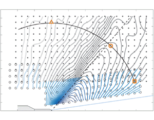
Figure 5 identifies the locations of all measurement points visited by the traversing system to map out the jet's acoustic field. This was accomplished by systematically traversing array  $\mathcal {A}$ in the positive axial direction, from position $i = 1$ to $i = 23$, in increments of 7 in. (0.178 m). Doing so allowed the 12-microphone array (identified by solid dots in figure 5 and labelled $j = 1, \ldots , 12$) to cover a rectangular grid. For each axial station between $i = 7$ and $i = 23$, array $\mathcal {B}$, with the five microphones identified by open circles in figure 5 and labelled $j = 13, \ldots , 17$, was traversed to a new radial position to follow the jet's growing shear layer. The growth rate is approximated to be $\Delta r/\Delta x = 1/7$, based on shadowgraphy images from Murray & Lyons (Reference Murray and Lyons2016) using the same nozzle and operating conditions. As a result of this set-up, acoustic pressure time series are recorded at a total of $23 \times 17 = 391$ points covering shallow, sideline and steep angle observer positions, relative to the prominent source field.

Figure 5. Dots and open circles identify measurement points covered by the microphone array. A total of  $i = 1, \ldots , 23$ locations were covered in the axial direction. At each $i$ location, data were acquired using array $\mathcal {A}$ (microphones $j = 1,\ldots , 12$, solid dots) and array $\mathcal {B}$ (microphones $j = 13, \ldots , 17$, open circles). A solid blue line identifies an approximate growth of the jet shear layer base on $\Delta r/\Delta x = 1/7$. Contours of overall sound pressure level (OASPL; in dB with $p_{ref} = 20\ \mathrm {\mu }\textrm {Pa}$) are shown in grey (array $\mathcal {A}$) and blue (array $\mathcal {B}$). The highest contour level is valued at 152 dB and resides closest to the shear layer. Subsequent contour levels are $-1$ dB with the lowest contour being 120 dB. The dashed line represents a reference Mach angle of $\phi _{ca} = 50^{\circ }$. The three grid points at $(x,r)/D_j \approx (49,18)$, $(35,39)$ and $(0,53)$, with square, round and triangle markers, respectively, identify locations where acoustic spectra are generated and displayed in figure 7.
2.3.2. Microphone acquisition and preprocessing
An assortment of  ${1}/{4}$ in. (6.35 mm) microphones were used in this study and were oriented so that their diaphragms were at grazing incidence to the acoustic wave fronts; similar set-ups were used by Viswanathan (Reference Viswanathan2006), Baars & Tinney (Reference Baars and Tinney2014) and Fiévet et al. (Reference Fiévet, Tinney, Baars and Hamilton2016). This orientation avoids having to point the normal vector of the diaphragm in the direction of the sound source, which is unambiguous for an elongated jet noise source. However, for free-field microphones, this requires a correction for the grazing orientation due to the intrusiveness and form factor of the microphone ( $90^{\circ }$ incidence waves). In all cases, microphone grid caps were removed to prevent high-frequency interference. A total of three different microphone types were used and were interlaced with one another as follows.
(i) Positions $j = 1, 3, \ldots , 7, 9, 10$ and 12 (array $\mathcal {A}$): Brüel & Kjaer (B&K) type 4939, free-field ${1}/{4}$ in. (6.35 mm) microphones, with a nominal sensitivity of $4\ \textrm {mV}\ \textrm {Pa}^{-1}$, a frequency response of up to 100 kHz and a dynamic range of up to 164 dB. (The acoustic definition of dB is used throughout with a reference pressure of $p_{ref} = 20\ \mathrm {\mu }\textrm {Pa}$.)
(ii) Positions
$j = 2$, 8 and 11 (array $\mathcal {A}$): Larson Davis model 2520, free-field ${1}/{4}$ in. (6.35 mm) microphones, with a nominal sensitivity of $4\ \textrm {mV}\ \textrm {Pa}^{-1}$, a frequency response of up to 80 kHz and a dynamic range of up to 164 dB.(iii) Positions
$j = 13, \ldots , 17$ (array $\mathcal {B}$): PCB model 112A22, high-resolution ${1}/{4}$ in. (6.35 mm) pressure probes, with a nominal sensitivity of $1.43 \times 10^{-2}\ \textrm {mV}\ \textrm {Pa}^{-1}$ and a resonance frequency $\geqslant 250$ kHz. Typically, the frequency response is valid up to at least 20 % of the resonance frequency (PCB, personal communication), meaning that the effective frequency response is 50 kHz. These pressure probes have a full-scale measurement range of 50 psi, resulting in a dynamic range of up to 205 dB.


All B&K and Larson Davis microphones were connected to B&K 2670 preamplifiers and powered by a B&K 2822 multiplexer. PCB probes were powered by a PCB 481 unit with a gain multiplier of 10. All 17 channels of data were digitized using two National Instruments (NI) PXIe-4497 cards embedded in a PXIe-1062Q chassis. These cards comprise built-in low-pass anti-aliasing filters with synchronized acquisition set to a rate of 200 kHz with 24-bit resolution ( ${\pm }5$ V). For in situ calibration, each microphone was checked using a B&K 4228 pistonphone (factory calibrated and certified, autumn 2019) with the appropriate sound pressure level (SPL) correction from a UZ0004 barometer. Insignificant differences were found from the manufacturer-specified calibration sensitivity, hence the latter were used to convert voltage signals to pascals.
At each microphone position, three statistically independent blocks of  $2^{19}$ samples were acquired, yielding a total of $T \approx 7.86$ s of data per position (or $TU_j/D_j \approx 1.27 \times 10^{5}$ turnover times). It was confirmed that this acquisition length was more than sufficient for obtaining converged spectral statistics at the lowest frequencies of interest. For all spectra shown here, the one-sided spectrum is taken as
 \begin{equation} G_{pp}(x,r;f) = 2\langle P(x,r;f) P^{*}(x,r;f)\rangle, \end{equation}
where  $P(x,r;f) = \mathcal {F}[p(x,r,t)]$ is the temporal fast Fourier transform (FFT), $^{*}$ signifies the complex conjugate and the angular brackets denote ensemble averaging. Acoustic spectra are presented as sound pressure spectrum level (SPSL) in dB following
 \begin{equation} \textrm{SPSL}_{m}(x,r;f) = 10\log_{10} (G_{pp}(x,r;f)/p^{2}_{ref}), \end{equation}
where subscript  $m$ refers to the raw measured values. Ensemble averaging was achieved using FFT partitions of $N = 2^{14}$ samples with a Hanning window (albeit the effect of window functions on these kinds of signals is negligible). The value of $N$ results in a spectral resolution of $\textrm {d}f = 12.2$ Hz for a total of 189 ensembles using 50 % overlap. Spectra are presented in dimensionless form using a Strouhal number defined by ${St} \equiv f/f_c$, and with a characteristic frequency valued at $f_c \equiv U_j/D_j \approx 16.12$ kHz.
During preprocessing stages of the analysis, two corrections were applied to the measured  $\textrm {SPSL}_m$ to arrive at a loss-less SPSL. The expression for this is provided in (2.5) where it is shown to comprise two parts, a free-field microphone correction to account for the grazing incidence of the sound field, followed by corrections for atmospheric absorption in accordance with ANSI standard S1.26-1996:
 \begin{equation}
\textrm{SPSL}(x,r;f) =
\underbrace{\textrm{SPSL}_{m}(x,r;f)}_{\text{measurement}}
+ \underbrace{\bar{\beta}_{j =
1-12}(f)}_{\text{free-field corr.}} +
\underbrace{\rho\bar{\alpha}_{j =
1-17}(f)}_{\text{atm. abs. corr.}}.
\end{equation}
\begin{equation}
\textrm{SPSL}(x,r;f) =
\underbrace{\textrm{SPSL}_{m}(x,r;f)}_{\text{measurement}}
+ \underbrace{\bar{\beta}_{j =
1-12}(f)}_{\text{free-field corr.}} +
\underbrace{\rho\bar{\alpha}_{j =
1-17}(f)}_{\text{atm. abs. corr.}}.
\end{equation}
The free-field correction,  $\bar {\beta }(f)$, is shown in figure 6(a) along with two microphone response curves for nominal sound wave incidence angles of $0^{\circ }$ and $90^{\circ }$, relative to the normal vector of the diaphragm. Free-field microphones ( $\kern1.5pt j = 1, \ldots , 12$) are designed for a nominal incidence of $0^{\circ }$. Here, the microphones were arranged with $90^{\circ }$ grazing incidence, so the free-field correction is applied, which adds back the attenuated energy in the signal. This portion of the signal's energy is highlighted by the grey hatched area in figure 6(a) the magnitude of which is identified by a dashed line ( $\bar {\beta }$).

Figure 6. (a) Method for calculating free-field microphone correction. (b) Sample atmospheric absorption correction curve  $\bar {\alpha }$. (c) Sound pressure spectrum level (SPSL) at $(x,r)/D_j = (35,39)$. The overall sound pressure level (OASPL) values provided correspond to spectral integrations between the vertical dashed lines at $f = 200$ Hz and $f = 60$ kHz. The 28 logarithmically spaced lines in the range $0.05 \leqslant {St} \leqslant 3$ identify the centre Strouhal numbers for the analysis described in § 3.1.
Corrections for atmospheric absorption,  $\bar {\alpha }$, identified as the third term on the right-hand side of (2.5), ensures that attenuation of the propagating pressure wave, due to molecular relaxation and thermoviscous absorption, is recovered. This requires a propagation distance $\rho = \sqrt {x^{2} + r^{2}}$ and an absorption coefficient $\bar {\alpha }$ in terms of dB per unit distance and is applied to all microphones ( $\kern1.5pt j = 1, \ldots , 17$). The correction is shown in figure 6(b) based on average chamber conditions ( $p_\infty$, $T_\infty$ and relative humidity RH) observed during the measurements. Note that the propagation distance for the atmospheric absorption correction, $\rho$, is the polar distance from the nozzle exit to the measurement location per figure 1(b). Hence, this assumes (solely for this correction) that the noise source is located at the nozzle exit. Both corrections primarily affect frequencies above 10 kHz, as can be seen from the sample spectrum plotted in figure 6(c). Here a filtered SPSL is shown using the black line (calculated using a ${\pm }20\,\%$ bandwidth moving filter) superposed on its raw spectral estimate in greyscale.
2.4. General characteristics of the acoustic far field
The spatial topography of the overall sound pressure level (OASPL) is shown in figure 5 and confined to a band of frequencies between 200 Hz and 60 kHz per (2.6), where  $\textrm {SPSL}(x,r;f)$ is the corrected spectrum using (2.5):
 \begin{equation} \textrm{OASPL}(x,r) = \int_{200\ \textrm{Hz}}^{60\ \textrm{kHz}} \textrm{SPSL}(x,r;f) \, \textrm{d}f. \end{equation}
Subtle differences were observed in the microphone outputs above 60 kHz, which are eliminated from the OASPL calculation by way of this high-frequency cutoff.
A two-dimensional spline interpolation in Matlab was then used to refine the number of grid points by a factor of 7 in both  $x$ and $r$. No noticeable differences between the original and linearly interpolated points were observed, which suggests that the original grid sufficiently captured changes in the sound field for the regions measured. In figure 5, a steep gradient in the OASPL along $\phi \approx 50^{\circ }$ reinforces the notion that the main lobe in this contour is due to Mach wave radiation; the intensity of these highly directional sound waves decays rapidly upstream of the Mach cone. Similar findings for supersonic jets have been reported by others (McLaughlin et al. Reference McLaughlin, Morrison and Troutt1975; Gallagher & McLaughlin Reference Gallagher and McLaughlin1981; Varnier Reference Varnier2001; Greska et al. Reference Greska, Krothapalli, Horne and Burnside2008; Baars & Tinney Reference Baars and Tinney2014).
Sample spectra are shown to reveal the unique distribution of frequencies that make up the OASPL at various locations in the far field. These are displayed in figure 7 and correspond to the three points identified by the square, round and triangle markers placed on an arc of radius  $\rho \approx 53D_j$ in figure 5. Figures 7(a) and 7(c) are located at shallow and steep angles to the jet axis, respectively, whereas the spectrum in figure 7(b) is located along the peak OASPL path with a peak at ${St} \approx 0.18$. It is known that this peak is associated with the jet's primary flow instability and will be referred to hereafter as the characteristic Strouhal number of the jet, and labelled ${St_c}$ in table 1. Shallow and steep angle observers, relative to the peak OASPL path, are shown to peak at lower and higher ${St}$ numbers, respectively. These shapes resemble the large-scale similarity and fine-scale similarity spectra proposed by Tam et al. (Reference Tam, Golebiowski and Seiner1996) and commonly referred to throughout the jet noise literature.

3. Frequency-dependent source fields
3.1. Methodology
Jet turbulence manifests a broad range of spatial and temporal scales that exchange energy through the mean flow while evolving downstream. Because radiating pressure waves are produced by the change in the turbulent sources of noise as they convect through the flow, then they too should carry a footprint of the spectral make-up of the source field. Numerous efforts to infer information about the phase and structure of the source field by probing signatures in the near-field pressure are found in studies by, for example, Arndt et al. (Reference Arndt, Long and Glauser1997), Picard & Delville (Reference Picard and Delville2000), Kerhervé, Fitzpatrick & Jordan (Reference Kerhervé, Fitzpatrick and Jordan2006), Suzuki & Colonius (Reference Suzuki and Colonius2006), Tinney & Jordan (Reference Tinney and Jordan2008) and Murray & Lyons (Reference Murray and Lyons2016). When the convective acoustic Mach number is supersonic, then Mach waves become the dominant sound-generating mechanism, as opposed to turbulent structures that form acoustically matched spatial flow patterns capable of radiating noise by way of a wavy wall analogy. Because Mach waves refract and coalesce to form distinct directivity patterns, then measurements beyond the hydrodynamic periphery of the jet flow, where pressure waves are purely acoustic, can be used to infer information about the source field. In what follows, an analysis of the spatially and temporally resolved sound field is carried out by systematically isolating a total of  $b = 1, \ldots , 28$ octave-type frequency bins (or Strouhal-number bins), logarithmically spaced across the range $0.05 \leqslant {St} \leqslant 3$. Figure 6(c) illustrates the centres and widths of these 28 bins, superimposed on the sample spectrum using a colour scheme that changes sequentially from yellow to red (low to high centre frequencies). The process for computing the energy in each of these bins mirrors that of a notch filter,
 \begin{equation} \textrm{SPSL}_{b}(x,r;{St}_{b}) = \frac{1}{\displaystyle\int_{{St}_{b,l}}^{{St}_{b,u}} \textrm{d}{St}}\ \underbrace{\int_{{St}_{b,l}}^{{St}_{b,u}} \textrm{SPSL}(x,r;{St}) \, \textrm{d}{St}}_{\textrm{SPL}(x,r;{St}_b)}, \end{equation}
where  ${{St}_{b,l}}$ and ${{St}_{b,u}}$ are the lower and upper bounds of bin $b$, and the SPL is the acoustic energy within bin $b$. Similar treatment methods have been used by Kuo et al. (Reference Kuo, Veltin and McLaughlin2012) and Baars et al. (Reference Baars, Tinney, Wochner and Hamilton2014).
Filtering the data this way produces an  $\textrm {SPSL}_{b}(x,r;{St}_{b})$ contour, as shown in figure 8(a) for $b = 10$ ( ${St}_{10} \approx 0.20$) as an example. This filtered field reveals a directivity pattern much like the original OASPL shown in figure 5. Field lines, corresponding to gradients in the SPSL contour shown in figure 8(b), are then drawn to highlight directions perpendicular to the SPSL contour lines and the formation of a gradient-based ridge. Field lines that track the gradient-based ridge are then identified, as shown in figure 8(c). A straight line is drawn, fitted to each of the gradient-based ridges, and is repeated for all gradient-based field lines that follow the dominant ridge. This is shown in figure 8(d) for a range of linear fit lines separated by differences in intensity of the blue-coloured curves, depending on what portion of the ridge is used. Each line accounts for a larger radial range to calculate the fit (up to each of the 10 blue markers). The process is automated so that it can be easily repeated for all 28 bins. A sample set of results is shown in figure 9(a–f) for six of the 28 available Strouhal-number bins studied and for frequencies below and above ${St}_c$.

Figure 8. (a) Spatial map of  $\textrm {SPSL}_{10}(x,r;{St}_{10})$, with ${St}_{10} \approx 0.20$, captured using microphone array $\mathcal {B}$. The highest contour level corresponds to 112 dB, residing closest to the shear layer, while each subsequent contour is $-1$ dB. (b) Perpendicular gradient field lines of the SPSL contour in panel (a). (c) Identification of the gradient field line that tracks the ridge in the SPSL contour. (d) Linear fits to the gradient field line of panel (c).

Figure 9. (a,b) Spatial maps of  $\textrm {SPSL}_{b}(x,r;{St}_{b})$ for the six bin numbers indicated. Linear fit lines of the ridges identified in the SPSL contours are superposed and extrapolated towards the jet axis.
For each of the six Strouhal-number bins shown in figure 9(a–f), a number of source characteristics are computed. Foremost, linear fit lines are extrapolated towards the jet flow in order to approximate the axial location of the source for a given frequency; for now, these sources are assumed to reside at a point where the linearly extrapolated line intersects the nozzle centreline at  $r=0$. The angle of each linear fit line, relative to the jet axis, is then computed and is denoted by $\phi _s$. Each angle approximates a frequency-dependent Mach wave radiation angle, which yields a convection velocity using $U_c = a_{\infty }/\cos (\phi _s)$. In general, the shapes of these contours are similar, though closer inspection reveals how the width of the ridge narrows with increasing frequency; higher frequencies are increasingly directive relative to lower frequencies. For Strouhal numbers higher than 0.18, the peak radiation angle coincides with the Mach wave radiation angle, while SPSL ridges shift upstream.
3.2. Results: source location and peak-intensity angle
Having compiled axial source locations, Mach wave radiation angles and their respective convection velocities, the findings are shown in figures 10 and 11 for all 28 Strouhal-number bins. Axial source locations are shown first in figure 10(a) alongside various findings from the literature (Tester et al. Reference Tester, Morris, Lau and Tanna1978; Papamoschou & Debiasi Reference Papamoschou and Debiasi1999; Dougherty & Podboy Reference Dougherty and Podboy2009; Kuo et al. Reference Kuo, Veltin and McLaughlin2012). The trend is very convincing. That is, lower frequencies point towards sources located farther downstream, while higher frequencies point towards regions closer to the jet exit. The shift in frequency is known to be caused by a considerable drop in axial phase velocity of the instability waves for low frequencies (Troutt & McLaughlin Reference Troutt and McLaughlin1982), and is a hallmark feature of high-Reynolds-number jet flows. Also, for each frequency, the distribution of markers in figure 10(a), as it relates to the spread amongst linear fit lines, is much tighter near  ${St_c}$ and is centred on an axial source located around $x_s/D_j = 8$ (the location is based on the intersection of the extrapolated lines in figure 9 with the nozzle centreline). This demonstrates how the characteristic source events are concentrated over a narrow region in space, relative to lower- and higher-frequency source events, and that the consequence of their compact nature is what makes them the characteristic source events of the flow. In figure 10(b), propagation angles are shown to range from approximately $35^{\circ }$ for low $St$ numbers, to a peak around $58^{\circ }$ at three times the value of ${St_c}$. Gradual levelling off of these propagation angles for higher frequencies is complementary to the findings of Kuo et al. (Reference Kuo, Veltin and McLaughlin2012), who showed that the angular orientation of the sound pressure intensity lobe remains mostly unchanged for frequencies greater than the characteristic Strouhal number. According to figure 10(b), the propagation angle corresponding to ${St_c}$ is valued at $50^{\circ }$, and reinforces earlier estimates based on Oertel (Reference Oertel1980).

Figure 10. (a) Axial source location (jet centreline intercept of the linear fit lines as illustrated in figure 9) versus  ${St}$, compared to trends from the literature (Kuo et al. Reference Kuo, Veltin and McLaughlin2012; Tester et al. Reference Tester, Morris, Lau and Tanna1978; Dougherty & Podboy Reference Dougherty and Podboy2009; Papamoschou & Debiasi Reference Papamoschou and Debiasi1999). (b) Peak propagation angle versus ${St}$.

Figure 11. (a) Convection velocity versus  ${St}$, compared to the trend of Veltin et al. (Reference Veltin, Day and McLaughlin2011). (b) Convection velocity versus axial source location, plotted from the data in figures 10(a) and 11(a). Superposed on this is the centreline velocity profile inferred from Pitot-static pressure and total temperature measurements, described in Appendix A.
Under the simplification that the peak-intensity angle of the noise is a function of the convection velocity only, a characteristic convection velocity can be inferred from  $U_c = a_\infty /{\cos (\phi _s)}$ following the simple model of figure 1(a). Most direct measurements report ratios ranging between 0.7 and 0.8 of the jet exit velocity (e.g. Norum & Seiner Reference Norum and Seiner1982; Troutt & McLaughlin Reference Troutt and McLaughlin1982; Tinney, Ukeiley & Glauser Reference Tinney, Ukeiley and Glauser2008). Similar discrepancies were recorded by Seiner et al. (Reference Seiner, Ponton, Jansen and Lagen1992). In figure 11(a), it is clear that lower frequencies coincide with lower convection velocities, which reside both upstream and downstream of the prominent source region, according to figure 11(b), and that all frequencies comprise supersonic convective acoustic Mach numbers. Take note of the fact that figure 11(b) is created by combining figures 10(a) and 11(a), and that the $x$-axis in figure 11(b) is the axial location corresponding to the intersection of extrapolated lines in figure 9 with the nozzle lip line at $r = 0.5D_j$ (whereas the nozzle's centreline was used in figure 10a).
These regions coincide with the growth and decay envelope of the jet's primary flow instability, respectively, with a saturation point residing around  $x_s/D_j = 8$. This location is just downstream of the region where the potential core collapses (identified at $x_c/D_j \approx 6.3$ in figure 22 of Appendix B).
The impediment to inferring convection velocities (associated with the source field) from acoustic signatures (registered in the far field) is that the former are dependent on both axial and radial locations in the flow, owing to the fact that jets are three-dimensional, but azimuthally invariant in an average sense. Ko & Davies (Reference Ko and Davies1971), Kerhervé et al. (Reference Kerhervé, Jordan, Gervais, Valière and Braud2004) and Fiévet et al. (Reference Fiévet, Tinney, Murray, Lyons and Panickar2013) have all shown that convection velocities are faster than the mean flow in the outer low-speed entrainment regions of the jet shear layer, while they are slower than the mean flow in the inner high-speed regions. Since these regions of the flow are dominated by the large scales, numerous efforts to construct conceptual models of jet turbulence have been performed using reduced-order modelling techniques capable of stripping away incoherent features responsible for obscuring the large-scale dynamics. These reduced-order models have shown that, for a range of subsonic Mach numbers and Reynolds numbers, the inner high-speed regions are characterized by organized column mode ( $m=0$) and helical mode ( $m=1$) structures, while the outer low-speed entrainment regions are dominated by higher azimuthal mode ( $m=5$) structures (Glauser & George Reference Glauser and George1987; Citriniti & George Reference Citriniti and George2000; Taylor, Ukeiley & Glauser Reference Taylor, Ukeiley and Glauser2001; Iqbal & Thomas Reference Iqbal and Thomas2007; Tinney et al. Reference Tinney, Ukeiley and Glauser2008).
Several efforts to understand the underlying relationship between the dominant structural modes in the flow have been performed. For example, Citriniti & George (Reference Citriniti and George2000) and Tinney et al. (Reference Tinney, Ukeiley and Glauser2008) revealed how the collapse of the potential core, where the dominant noise sources reside, manifests volcano-like eruptions comprising high-strain, short-duration events driven by column mode and helical mode structures in the flow. The helical mode is interpreted as being the result of a misalignment of the jet column mode structure with the jet axis, thereby resulting in an axial phase shift in the  $m=0$ mode. Iqbal & Thomas (Reference Iqbal and Thomas2007) showed the jet shear layer to comprise sequences of fast-moving toroidal shear layer vortices connected to one another by way of slower-moving vortical braids in the outer regions of the jet.
Thus, while the underlying mechanisms that govern jet turbulence are quite complex and are a manifestation of numerous scales that evolve both axially and radially, our current survey of the acoustic field offers an opportunity to distil general information concerning the sources of turbulence mixing noise, and without all the fuss. From figure 11(b), one can see that convection velocities increase uniformly along the growth regions of the jet from  $U_c/U_j \approx 0.62$ to a maximum around 0.78. After the collapse of the potential core, convection velocities continue to slow, and in regions where column mode and helical modes dominate the azimuthal structure of the jet turbulence. This reinforces the notion that the primary sources of noise for Mach wave radiation are likely to be the column mode and helical mode structures (similar to the findings of Tam & Burton (Reference Tam and Burton1984)), which reside on the high-speed sides of the shear layer and that break apart while erupting from the collapsing of the potential core.
4. Frequency-dependent data-informed polar patterns
4.1. Source directivity
It is understood that the acoustic far field of a jet is where pressure waveforms spread spherically and decay according to  $p \propto 1/\rho$, where $\rho$ is the distance from the source according to figure 1(b). This is true for both the entire acoustic pressure waveform as well as individual frequencies that collectively make up the full waveform. Thus, if a pressure waveform is purely acoustic, then one should be able to match identically the statistical variance between a near-field and far-field observer using the inverse square law, so long as the source location, amplitude and propagation path are known. A sketch of this is shown in figure 12 for the ${St}_{12} \approx 0.27$ bin as an example. Increases in colour intensity correspond to increases in distance from the source, while the data-informed source location, for this particular frequency, is inferred from the results of figure 10(a). Given the complexity of the near field due to coalescence and hydrodynamic effects, only points satisfying $\rho _s > 20D_j$ are projected along rays to the far-field observer identified in figure 12 as an arc at $\rho ^{*}_s = 60D_j$ from the source. The calculation is quite trivial and is written as
 \begin{equation} \textrm{SPSL}_{b,{S}}(\rho^{*}_s,\phi_s;{St}_b) = \textrm{SPSL}_{b}(\rho_s,\phi_s;{St}_b) + 20\log_{10}\left(\frac{\rho^{*}_s}{\rho_s}\right). \end{equation}
 Now, if one were to assume that all sources (corresponding to all frequencies) were to reside at the nozzle exit ( $x = 0$), the following calculation would be performed to recover the polar pattern along an arc with radius $\rho ^{*} = 60D_j$:
 \begin{equation} \textrm{SPSL}_{b,{N}}(\rho^{*},\phi;{St}_b) = \textrm{SPSL}_{b}(\rho,\phi;{St}_b) + 20\log_{10}\left(\frac{\rho^{*}}{\rho}\right). \end{equation}
Note the subscripts  $S$ and $N$ in the formulations above, which refer to data-informed and nozzle-centred source locations, respectively. The results of these projections, using two different methods based on (4.1) and (4.2), are displayed in figure 13(a–f) for three Strouhal-number bins (below and above ${St_c}$), and over a broad range of observer angles. Similar analyses were presented by Kuo et al. (Reference Kuo, Veltin and McLaughlin2012) and Fiévet et al. (Reference Fiévet, Tinney, Baars and Hamilton2016), but for OASPL, as opposed to the discrete frequencies considered here. Corrections for atmospheric absorption were applied to all data, while changes in colour intensity follow the same ritual used in figure 12.

Figure 12. Illustration of all measurement points (blue-coloured) used to project  $\textrm {SPSL}_{12}(x,r;{St}_{12})$ to an arc at $\rho ^{*}_s = 60D_j$ and centred at its unique source location. Points with a polar distance $\rho _s < 20D_j$ (grey-coloured) are omitted in this procedure.

Figure 13. (a,c,e)  $\textrm {SPSL}_{b,{S}}(x,r;{St}_{b})$ polar patterns corresponding to Strouhal-number bins 4, 12 and 20, projected to an arc at $\rho ^{*}_s = 60D_j$ following figure 12. Solid thick lines identify the average of all polar patterns; dashed lines represent the spread of data using the r.m.s. of data points above and below the mean. (b,d,f) Similar to panels (a,c,e), but now $\textrm {SPSL}_{b,{N}}(x,r;{St}_{b})$ is the polar projection to an arc at $\rho ^{*} = 60D_j$, assuming all sources reside at the nozzle exit plane.
Starting with the results of the nozzle-based projection  $\textrm {SPSL}_{b,{N}}$ in figure 13(b,d,f), all data are shown to comprise a wide range of scatter and illustrate how a seemingly simple spherical extrapolation from a nozzle-centred source produces erroneous far-field predictions. Closer inspection reveals how the scatter decreases with increasing frequency (15 dB for ${St}_{b} = 0.08$, followed by 5 dB for ${St}_{b} = 0.89$). On the contrary, when data-informed source locations are used, sound pressure levels $\textrm {SPSL}_{b,{S}}$ are shown in figure 13(a,c,e) to collapse well. The average of all data points for a given Strouhal-number bin is drawn with a solid line, computed using a sliding window average comprising an angular width of $\Delta \phi _s = 5^{\circ }$. Dashed lines on either side of the solid line indicate the root mean square (r.m.s.) of all data points (separate for data points above and below the average solid line). Deviations in the dashed lines, relative to the average, are small, thereby reinforcing the use of data-informed source locations for collapsing far-field pressure signatures on a per-Strouhal-number-bin basis.
We expand upon this finding in figure 14, where SPSL polar patterns are projected to an arc at  $\rho _s^{*} = 60D_j$ using (4.1) with all measurement points and for 10 Strouhal-number bins ranging from 0.05 to 3.0 (bin numbers $b = 1$, 3 and 28). Data corresponding to bin 1 (lowest ${St}$ number) are presented with the lightest shade of colour (yellow), while subsequent polar patterns are offset by $-5$ dB in order to reduce clutter. Each polar pattern comprises a solid thick line to denote the average of all data points, (post-projection and using the same sliding window average spanning segments of $\Delta \phi _s = 5^{\circ }$), which was presented earlier in figure 13(a,c,e) using a subset of the bins shown here. The lighter envelope surrounding the solid line indicates the bounds set by the r.m.s. envelope of all data points (described previously). For all data-informed polar patterns, and thus for the entire Strouhal-number range studied ( $0.05 \leqslant {St} \leqslant 3$), the values corresponding to individual polar patterns are nearly identical to the average value. This result demonstrates the significance of using data-informed and frequency-dependent source locations to collapse far-field pressure signatures, even for low- and high-frequency waveforms that venture from the peak Strouhal number of the jet.

Figure 14.  $\textrm {SPSL}_{b,{S}}(x,r;{St}_{b})$ polar patterns at $\rho ^{*}_s = 60D_j$ for 10 Strouhal numbers, corresponding to bins $b = 1$, 3 and 28. The solid thick lines identify the average polar pattern; envelopes represent the spread from the r.m.s. of data points while subsequent polar patterns are offset by $-5$ dB (from yellow to red).
4.2. Estimating sound pressure spectrum levels in the acoustic far field
Given the frequency-dependent polar patterns  $\textrm {SPSL}_{b,{S}}(\rho ^{*}_s,\phi _s;{St}_{b})$ in figure 14, and their corresponding axial source locations $x_s({St}_b)$ in figure 10(a), the acoustic spectra in the far field of a full-scale supersonic jet, using laboratory-scale measurements of geometrically identical hardware, can be accurately predicted in a straightforward manner (and was used for noise exposure modelling by Pedersen, Murray & Baars (Reference Pedersen, Murray and Baars2020)). For each Strouhal-number bin, SPSL magnitudes are projected to any new location of interest $(\tilde {x}, \tilde {r})$ using the equation
 \begin{equation}
\textrm{SPSL}{}^{pred}_{b}(\tilde{\rho}_s,\tilde{\phi}_s;{St}_b)
= \textrm{SPSL}_{b,{S}}(\rho^{*}_s,\tilde{\phi}_s;{St}_b)
+
20\log_{10}\left(\frac{\rho^{*}_s}{\tilde{\rho}_s({St}_b)}\right).
\end{equation}
\begin{equation}
\textrm{SPSL}{}^{pred}_{b}(\tilde{\rho}_s,\tilde{\phi}_s;{St}_b)
= \textrm{SPSL}_{b,{S}}(\rho^{*}_s,\tilde{\phi}_s;{St}_b)
+
20\log_{10}\left(\frac{\rho^{*}_s}{\tilde{\rho}_s({St}_b)}\right).
\end{equation}
The projection accounts for spherical spreading on account of the directivity pattern that is unique to each Strouhal-number bin and for characteristic locations of the source. According to figure 1(b) the polar coordinates of the newly projected location are defined by  $\tilde {\rho }_s({St}_b) = \sqrt {(\tilde {x} - x_s({St}_b))^{2} + \tilde {r}^{2}}$ and $\tilde {\phi }_s({St}_b) = \tan ^{-1}[\tilde {r}/(\tilde {x} - x_s({St}_b))]$.
A demonstration of this is shown in figure 15(a), where the predicted SPSL, at a sample location of  $(\tilde {x},\tilde {r}) = (200,200)D_j$, is presented for all discrete frequency bins. Error bars are drawn to identify the r.m.s. of each frequency bin, given the culmination of errors from the polar patterns presented in figure 14. A reference spectrum, identified by a grey line in figure 15(a), represents the spectrum predicted at $(\tilde {x},\tilde {r}) = (200,200)D_j$ using all resolved frequencies measured at $(x,r) = (35,35)D_j$ and by assuming a $45^{\circ }$ propagation path emanating from the nozzle exit plane at $(x,r) = (0,0)$. The measurement at $(x,r) = (35,35)D_j$ corresponds to a radial distance of $\rho _{I} = 49.5D_j$ and a polar angle of $\phi _{I} = 45^{\circ }$, relative to the nozzle exit, so that the reference spectrum is calculated from $\textrm {SPSL}^{pred}(\tilde {x},\tilde {r};{St}) = \textrm {SPSL}(x,r;{St}) + 20\log _{10}(\rho _{I}/\tilde {\rho })$. It is evident from this example how the reference spectrum underpredicts lower frequencies while overpredicting higher frequencies. This is traced to the assumption of a nozzle-centred source location used to obtain the reference spectrum and its failure to account for the elongated and frequency-dependent jet noise source field.

Figure 15. (a) Sound pressure bin spectrum estimated using frequency-dependent polar patterns with data-informed source locations (coloured points with error bars) alongside an estimate using the nozzle-centred method (grey line) as a reference. (b) Recasting panel ( $a$) using aerodynamic similarity for a full-scale jet diameter of $\tilde {D}_j = 0.5$ m. (c) Corrections to panel (b) for atmospheric absorption effects.
Geometric scaling (from laboratory scale to full scale) is then accounted for by using the Strouhal number such that  ${St} \equiv f \tilde {D}_j/U_j$. This assumes that jet flows are aerodynamically similar so that SPSL bands are placed over the proper range of frequencies. Figure 15(b) illustrates the spectra from figure 15(a) using a frequency label on the abscissa based on a theoretical full-scale jet exit diameter of $\tilde {D}_j = 0.5$ m. Corrections for atmospheric absorption using (4.4) are then applied, given that the jet exit diameter, and hence the absolute travel distance $\tilde {\rho }_s({St}_b)$ of the acoustic waves, are known for each Strouhal-number bin. The frequency-dependent absorption coefficient $\bar {\alpha }$ is applied to each SPSL bin with corresponding travel distances (assuming standard sea-level temperature and pressure, and a relative humidity of $\textrm {RH} = 60$ %) so that
 \begin{equation} \textrm{SPSL}^{\alpha,{pred}}_{b}(\tilde{\rho}_s,\tilde{\phi}_s;f_b) = \textrm{SPSL}^{pred}_{b}(\tilde{\rho}_s,\tilde{\phi}_s;f_b) - \tilde{\rho}_s\,\bar{\alpha}(f_b). \end{equation}
This post-absorption correction is presented in figure 15(c), where, once again, the values registered for each spectral bin are predicted on account of the correct source location for each frequency (similar to the approach employed by Kuo et al. (Reference Kuo, Veltin and McLaughlin2012)). One can see that the difference in OASPL (confined to the frequency range  $75\ \textrm {Hz} \leqslant f \leqslant 5285\ \textrm {Hz}$ as it corresponds to the full-scale system) is approximately 1.5 dB at $(\tilde {x},\tilde {r}) = (100,100)$ m and is accompanied by a noticeable shift in the peak frequency from 175 Hz to 326 Hz.
5. Errors in calculating far-field metrics
Figure 15 illustrates the kinds of discrepancies that are encountered when a nozzle-centred source is assumed for all frequencies, combined with an input location that is too close to the source field (an input location of  $\rho _I \approx 49.5D_j$ was used). This presents two issues, where errors associated with jet noise measurements are concerned. The first is at what distance from the nozzle centre is it safe for an observer to be considered in the geometric far field. The second is an understanding of the errors that one should expect to encounter when calculating common metrics such as SPSL and sound power level. These errors are now assessed using the approach outlined in the previous section.
5.1. Identifying the geometric far field of supersonic jets
The first question that we seek to address is at what distance does one consider the geometric far field to be so that the source field can be treated as compact. Ideally, one would want an answer that is universal for all jet operating conditions. Unfortunately, the effects of pressure ratio and temperature ratio on the convective acoustic Mach number and the length of the elongated source region make it difficult for a simple answer to come by. Albeit, the operating conditions of this nozzle resemble operating conditions of current propulsion hardware, and so the solutions drawn here should convey useful insight into other studies concerned with the noise from supersonic jets.
In figure 16(a,c,e), errors in the predicted SPSL, for three different Strouhal-number bins, are shown using data from an arc with a radius of  $\rho _a = 60D_j$ as the input, combined with a nozzle-centred projection. Error $\varepsilon$ in dB is here taken as the result of the nozzle-centred projection, minus the correct polar-pattern-based projection using (4.3). At angles above and below the data-informed propagation angle (for a given frequency bin), amplitudes are underpredicted and overpredicted, respectively, and by as much as 6 dB. Blue dash-dotted lines follow the ridges in figure 16(a,c,e) corresponding to peak negative errors. These errors are then portrayed as error magnitudes in figure 16(b,d,f) and with additional arcs located at $\rho _a = 40D_j$, $90D_j$ and $150D_j$ as input for the projections (the same blue dash-dotted line style is used in figure 16(b,d,f) for the $\rho _a = 60D_j$ arc). Here the abscissa is taken as the outward polar distance $\rho$, normalized by the input arc radius $\rho _a$. As expected, higher frequencies comprise the smallest errors when a nozzle-centred source is used. Likewise, the error is known to decrease when the input data to the nozzle-centred projection is taken at an artificial arc array with a larger radius $\rho _a$. That is, the errors reduce from approximately 4 dB to 2 dB, using ${St}_{12} \approx 0.27$ in figure 16(d) as an example, when the input measurement is changed from $40D_j$ to $90D_j$ and the projection distance is a factor of 2. Errors converge to their asymptotic values (identified by lines to the right of each panel), which decrease with increasing frequency, and with increasing radius of the nozzle-centred arc.

Figure 16. Differences between a nozzle-centred projection and projections based on frequency-dependent polar patterns, expressed as errors in dB and presented for (a)  ${St}_{4} \approx 0.08$, (c) ${St}_{12} \approx 0.27$ and (e) ${St}_{20} \approx 0.89$ using an arc located at $\rho _a = 60D_j$ as the input for the nozzle-centred projections. (b,d,f) Peak negative errors corresponding to the blue dashed lines drawn in panels (a,c,e) and for additional arcs located at $\rho _a = 40D_j$, $90D_j$ and $150D_j$ as input for the nozzle-centred projections.
Concentrating on the maximum over- and underprediction in the acoustic far field, the errors in the asymptotic values can now be assessed for all frequencies (or Strouhal-number bins) and as a function of the input arc radius  $\rho _a$. Figure 17(a) displays the maximum underprediction (e.g. some points in this contour correspond to the asymptotic values presented in the profiles in figure 16b,d,f), while figure 17(b) presents the maximum overprediction. Both contours provide guidance as to the location of the geometric far field (assuming a nozzle-centred source) for supersonic jets operating under realistic conditions. Focusing on the underpredictions of the characteristic Strouhal number of the jet in figure 17(a), if one is willing to accept an error of roughly ${\pm }3$ dB in SPSL levels, then a nozzle-centred arc with a radius of $\rho _a \approx 150D_j$ is sufficient. Tightening the criteria to ${\pm }1$ dB requires an arc radius of $\rho _a \approx 450D_j$. These kinds of distances are nearly impossible to come by in most laboratory testing facilities and reinforce the need for employing the kind of microphone set-up and data-processing methods used here to generate data-informed and frequency-dependent polar patterns.

Figure 17. Peak (a) negative and (b) positive errors  $\epsilon$ in dB (the asymptotic error taken as the result of the nozzle-centred projection, minus the correct polar-pattern-based projection), as a function of the nozzle-centred arc radius $\rho _a$ and for all the frequencies.
5.2. Jet acoustic power
Here we turn our attention to computing the acoustic power of the jet flow and its associated error, for which these polar patterns and characteristic source locations are also a prerequisite. Acoustic power (or sound power) is the rate per unit time at which acoustic energy is emitted by a source, and thus has units of joules per second or watts. In practice, the acoustic power  $P_{S}$ is calculated from the (time-averaged) sound intensity vector $\boldsymbol {I} \equiv \langle p(t) \boldsymbol {u}(t) \rangle _t$, which is the time-averaged rate of energy transmission per unit area (the subscript $t$ indicates time averaging). The component of the intensity vector that is normal to the surface, denoted $I_n$, must be integrated over that surface to obtain the acoustic power:
 \begin{equation} P_{S} = \int_A \boldsymbol{I} \boldsymbol{\cdot} \boldsymbol{n}\,\textrm{d}A = \int_A I_n\,\textrm{d}A. \end{equation}
 Given that the acoustic impedance is the ratio of acoustic pressure to particle speed, then  $I_n = (p_{rms}^2/(\rho a_\infty)) \cos(\xi)$, where $\xi$ is the angle between the direction of wave propagation (the acoustic intensity vector $\boldsymbol {I}$) and the unit vector normal to the surface. When the acoustic intensity vector is aligned with the unit vector normal to the surface, then the acoustic power is computed from just the r.m.s. pressure as
 \begin{equation} P_{S} = \int_A \frac{p^{2}_{rms}}{\rho a_{\infty}} \,\textrm{d}A. \end{equation}
 This scenario, for which  $\xi = 0^{\circ }$, is sketched in figure 18(b), and is displayed such that the spherical surface in the acoustic far field is centred on the location of the characteristic source. On a per-Strouhal-number-bin basis, this is the case for only one of the data-informed polar patterns with corresponding source locations shown earlier. Note that when the spherical surface is in the acoustic far field, but not centred on the characteristic source (say, centred at the nozzle exit in figure 18a), the angle $\xi$ is non-zero. Quite often, acoustic measurements are unaccompanied by any knowledge of the source field, or are fixed in place using a boom array of microphones centred on the nozzle exit. As such, the acoustic intensity vector is unknown so that (5.2) is used without imposing necessary corrections for the true source locations, which introduces errors into the acoustic power calculation. Acoustic intensity probes allow for an average intensity vector direction, but these types of measurements are also non-trivial (Jaeger & Allen Reference Jaeger and Allen1993).

Figure 18. Diagram of the acoustic intensity vector for a given source location. Scenarios when (a) a compact nozzle-centred source location is assumed and (b) a data-informed source location is considered.
Here, acoustic power is calculated using the scenario described in figure 18(b); this ensures that the acoustic intensities from pressure measurements are normal to the surface of integration. Far-field pressure terms  $p^{2}_{rms}$ in (5.2) are determined from the polar patterns, which were presented as $\textrm {SPSL}_{b,{S}}(\rho ^{*}_s,\phi _s;{St}_{b})$ in figure 14. Pressure variance, and thus acoustic power, involves integrations over both space and frequency. Spatial integrations are confined by polar angle segments of a sphere spanning the domain $\phi _s \in [\phi _{s1},\phi _{s2}]$ and with full revolutions in azimuth for each polar angle segment, $\theta \in [0,2{\rm \pi} )$. If one considers a sphere with radius $\rho ^{*}_s$ (polar patterns are prescribed at this radius from the data-informed source), the surface area alone is determined by
 \begin{equation} A = \rho^{*2}_s
\int_{0}^{2{\rm \pi}} \int_{\phi_{s1}}^{\phi_{s2}}
\sin(\phi_s) \, \textrm{d}\phi_s \,
\textrm{d}\theta = 2{\rm \pi} \rho^{*2}_s
\int_{\phi_{s1}}^{\phi_{s2}}
\sin(\phi_s)\,\textrm{d}\phi_s.
\end{equation}
\begin{equation} A = \rho^{*2}_s
\int_{0}^{2{\rm \pi}} \int_{\phi_{s1}}^{\phi_{s2}}
\sin(\phi_s) \, \textrm{d}\phi_s \,
\textrm{d}\theta = 2{\rm \pi} \rho^{*2}_s
\int_{\phi_{s1}}^{\phi_{s2}}
\sin(\phi_s)\,\textrm{d}\phi_s.
\end{equation}
Combining (5.2) and (5.3), the acoustic power (watts) associated with a single Strouhal-number bin  $b$ is computed as
 \begin{equation} P_{{S},b} = \frac{2{\rm \pi} \rho^{*2}_s}{\rho a_\infty} \int_{\phi_{s1}}^{\phi_{s2}} \sin(\phi_s) p^{2}_{rms}(\rho^{*}_s,\phi_s;{St}_b) \, \textrm{d}\phi_s. \end{equation}
In (5.4), the argument of the integral is the polar pattern of the pressure variance (presented as SPSL in figure 14), and is weighted by the term  $\sin (\phi _s)$ to account for the surface area of the sphere due to revolutions about $\theta$. Because the pressure variance is bin-integrated, the correct value (in pascal $^{2}$) is computed from
 \begin{equation} p^{2}_{rms}(\rho^{*}_s,\phi_s;{St}_b) = p_{ref}^{2} 10^{(\textrm{SPL}_b/10)}, \end{equation}
where  $\textrm {SPL}_b$ is the bin-integrated SPSL following (3.1). A simple summation then yields the total acoustic power for the full range of Strouhal numbers spanning all 28 bins,
 \begin{equation} P_{S} = \sum_{b = 1}^{28} P_{{S},b}, \end{equation}
so that the sound power level, or sound watt level (SWL), can be determined from the total acoustic power  $P_{S}$ as
 \begin{equation} \textrm{SWL}_{S} = 10\log_{10}\left(\frac{P_{S}}{P_0}\right). \end{equation}
The common reference power of  $P_0 = 10^{-12}\ \textrm {W} = 1\ \textrm {pW}$ is used to normalize the solution.
One can see that acoustic power is independent of the radius of the sphere over which integrations are performed. This is true so long as the polar directivity patterns of the pressure variance are in the acoustic far field of the jet, and that the acoustic intensity vector is normal to these patterns. This requires that the source location be identified for each frequency. Therefore, if one encloses a source with two spherical segments of two different radii, the rate per unit time of radiated acoustic energy through both of these surfaces must be equal. Equation (5.4) reinforces this since the value of  $\rho ^{*2}_s p^{2}_{rms}(\rho ^{*}_s,\phi _s;{St}_b)$ is invariant with respect to $\rho ^{*}_s$, given that the pressure variance is taken in the acoustic far field where the pressure decays according to $p^{2} \propto 1/\rho _s^{2}$. Thus, while polar patterns were presented for $\rho ^{*}_s = 60D_j$, the term $\rho ^{*2}_s p^{2}_{rms}(\rho ^{*}_s,\phi _s;{St}_b)$ is unique. This implies that the polar angle integration bounds can be taken as constants $\phi _{s1} = \phi _1$ and $\phi _{s2} = \phi _2$ (not varying with $b$) since, for $\rho ^{*}_s \rightarrow \infty$, the angular domains defined by a similar range in either $\phi$ or $\phi _s$ are indifferent.
Figure 19 presents the acoustic power for each Strouhal-number bin,  $P_{{S},b}$, where the boundaries of the polar angle domain are defined by $\phi _s = [20^{\circ },110^{\circ }]$. The peak acoustic power is shown to reside at a Strouhal number of ${St}_{12} \approx 0.27$, which differs from the characteristic Strouhal number for this jet. The discrepancy is attributed to differences in the geometric locations of the various frequency-dependent sources and their unique polar patterns, relative to a far-field observer.

Figure 19. Estimates of acoustic power produced by individual Strouhal-number bins.
The total acoustic power produced by this heated supersonic jet flow is calculated from (5.6) and is valued at  $P_S = 942.26$ W or $\textrm {SWL}_{S} = 149.74$ dB. The acoustic efficiency is then determined from the following formula:
 \begin{equation} \eta \equiv \frac{P_{S}}{0.5\dot{m}U_j^{2}}. \end{equation}
The denominator is the kinetic energy of the jet flow computed from the exit conditions, with  $\dot {m} = \rho _jU_j{\rm \pi} D_j^{2}/4$ being the mass flow. Thus, $\eta$ represents how much of the kinetic energy of the jet inflow is converted to acoustic energy radiating to the far field. For this jet $E_k = 202.73$ kW, yielding an acoustic efficiency of $\eta \approx 0.46\,\%$.
5.3. Errors in assuming a compact nozzle-centred source
The errors that one encounters when the jet's acoustic power is computed under the assumption of a compact nozzle-centred jet noise source can now be assessed. These errors assume that the true acoustic power is computed from frequency-dependent polar patterns with data-informed source locations. For this analysis, a series of nozzle-centred arc arrays were artificially created from the microphone grid data. As shown in figure 20(a), these arcs are centred on the nozzle exit plane and range from  $\rho /D_j = 20$ up to $\rho /D_j = 56$. The new acoustic power is calculated for a single Strouhal-number bin by modifying (5.4) so that it can be evaluated along nozzle-centred arcs as
 \begin{equation} P_{{N},b}(\rho) = \frac{2{\rm \pi}\rho^{2}}{\rho a_\infty} \int_{\phi_{1}}^{\phi_{2}} \sin(\phi)p^{2}_{rms}(\rho,\phi;{St}_b)\,\textrm{d}\phi, \end{equation}
where the subscript  $N$ is used to identify a nozzle-centred calculation, and the pressure variance is, once again, bin-integrated,
 \begin{equation} p^{2}_{rms}(\rho,\phi;{St}_b) = p_{ref}^{2} 10^{(\textrm{SPL}_b/10)}. \end{equation}
Figure 20. (a) Illustration of the smallest ( $\rho _a/D_j = 20$) and largest ( $\rho _a/D_j = 56$) nozzle-centred polar patterns used to compute the acoustic power by way of a nozzle-centred compact source. (b) Errors in the acoustic power using a nozzle-centred compact source, relative to the true acoustic power. Coloured lines correspond to the acoustic power for each Strouhal-number bin (yellow to red represent low to high ${St}_b$, $b = 1, \ldots , 28$). A black line identifies the total (summed) error.
For reasons described earlier, errors are introduced since acoustic power now comprises integrations of the pressure variance polar patterns centred on the nozzle exit, as well as misalignment of the acoustic intensity vector, relative to the unit normal vector, as shown in figure 18(a). Note that the acoustic power calculation following (5.9) now depends on the radius of the spherical surface of integration, since we know from the discussion in § 4.1 (and the description of figure 13b,d,f) that the far-field pressure amplitude does not spread spherically when one makes the incorrect assumption of a compact source located at the nozzle exit.
The findings from this analysis are shown in figure 20(b). Here, the nozzle-centred acoustic power, with curves of  $P_{{N},b}(\rho )$, are normalized by the true acoustic power $P_{{S},b}$ shown in figure 19(b). Coloured lines correspond to relative errors on a per-Strouhal-number-bin basis (yellow to red correspond to $b = 1, \ldots , 28$) while a black line identifies errors in the total acoustic power summed over all 28 frequency bins. It is evident that when the largest nozzle-centred radius is considered ( $\rho /D_j = 56$), relative errors in the acoustic power calculation are small (within roughly ${\pm }6$ %). However, because the acoustic power comprises integrations over space $\phi \in [20^{\circ },110^{\circ }]$, then it masks errors at isolated angles $\phi$. We know from previous analysis in § 4.1 that the pressure variance does not decay spherically from the nozzle exit outwards. This means that the polar pattern is unique for each polar distance $\rho$ (e.g. when inspecting figure 13d, the polar patterns at relatively large $\rho$ are formed by the darkest points, while polar patterns at low $\rho$ are formed by lighter points). Ambiguities in the polar patterns of the pressure variance cause the acoustic power calculations to be over- or underestimated at certain polar angles. Errors are less when $\rho$ is large relative to the mismatch in source location. As such, from figure 20(b), it is evident that when decreasing the radius of the nozzle-centred sphere, errors in the estimates of acoustic power increase. Low-Strouhal-number bins are primarily affected by this, since their source locations (and thus their primary locations of acoustic power radiation) are located furthest downstream. It is noted that at distances far from the jet, the acoustic power curves appear to be identical in value (when the relative error in figure 20(b) is 1), but this is merely a cancelling of errors during the integration between certain regions in the polar angle domain $\phi$ over which the integration is performed.
6. Concluding remarks
The focus of this effort is to establish the proper framework for sensing the sound produced by jet flows with distributed source field and is driven by a number of observations regarding the directivity pattern that forms from turbulent shear flows with supersonic convective acoustic Mach numbers. The impetus for this work is taken from Kuo et al. (Reference Kuo, Veltin and McLaughlin2012), Baars et al. (Reference Baars, Tinney, Wochner and Hamilton2014) and Fiévet et al. (Reference Fiévet, Tinney, Baars and Hamilton2016), where it is shown that, when the dominant turbulence mixing noise mechanism is from Mach waves, a nozzle-centred source fails to accurately scale the far-field acoustics for distances that are typical of most jet noise testing facilities. This is important for several reasons. As much of the motivation for studying jet noise is to validate numerical models, predict full-scale conditions and/or eventually identify practical means of control, differences of 2–3 dB are significant, which is greater than the tolerable levels of error in one's measurement apparatus. It is then surprising when such careful considerations are made to select instruments, check calibrations, measure their placement relative to a common reference point and apply corrections for absorption, when an even larger discrepancy is encountered if one propagates their measurement to a different observer using the wrong propagation path, or from measurements too close to the nozzle to assume that the source is compact. Given the heart-shaped directivity pattern that is emblematic of subsonic jets, it is believed that the same process described here could prove useful for subsonic jet flow measurements. In fact, the radiation pattern extremities that form for the supersonic case help to reinforce one's understanding of the patterns that form at lower, subsonic, Mach numbers.
Acknowledgements
The authors wish to acknowledge Mr S. O'Connor (Program Manager), Mr S. Keefe and Mr M. Rudy (NAVAIR PMA-265). We would also like to give special thanks to Dr P. Panickar, Mr A. Green and Mr J. Herlan for their assistance in performing the experimental measurements. We wish to offer a posthumous acknowledgment to Mr B.J. Jansen, whose contributions to the aero-acoustics studies at the NCPA cannot be overstated.
Funding
The authors are grateful for financial support from NAVAIR PMA-265.
Declaration of interests
The authors report no conflict of interest.
Appendix A. Details of the MOC nozzle
The shape of the supersonic nozzle contour employed in this study was designed using the method of characteristics for axisymmetric nozzles based on the computer program from Sivells (Reference Sivells1978). An illustration of the contour is shown in figure 21 and comprises a nozzle exit diameter of  $D_j = 1.90$ in. (48.3 mm), a throat diameter of $D^{*} = 1.74$ in. (44.2 mm) and thus an area ratio of $A_e/A^{*} = 1.202$. The design Mach number at the exit of $M_d = 1.5314$ assumes heated air as the working fluid with a ratio of specific heats of $\gamma = 1.365$. The radius of curvature at the throat is $0.78D_j$ while the overall length of the nozzle, from throat to lip, is $1.05D_j$.

Figure 21. Interior contour of the MOC nozzle with the exit-to-throat area ratio of  $A_e/A^{*} = 1.202$ and a jet exit diameter of $D_j = 48.3$ mm.
Appendix B. Potential core lengths
Following Baars et al. (Reference Baars, Tinney, Murray, Jansen and Panickar2011), a characteristic length scale corresponding to the turbulent mixing region of the jet is needed to scale the location and extent of the source region. Typically, one may use the exit diameter of the nozzle, the length of the potential core (defined by the region where  $U_{cl}\geqslant 0.95U_j$) or the length of the supersonic tip (where $M_{cl}\geqslant 1.0$). For supersonic flows, the last of these quantities is not easy to come by and requires some assumptions about the gas. Here, both a Pitot-static pressure probe and a total temperature probe were traversed along the jet's centreline and used as input to calculate Mach number, axial velocity and thermodynamic properties of the gas. Calculations were performed in an iterative fashion by assuming ideal gas properties and local thermodynamic equilibrium with $\gamma (T(x)) = 1.428 - (8.6282 \times 10^{-5}\,T)$, where $T$ is in kelvin. The behaviour of the heated air along the jet axis is presented in figure 22(a,b). From this, the end of the jet potential core is estimated as $x_c/D_j \approx 6.3$ and is based on the intersection of two straight lines used to characterize the centreline velocity $U_{cl}/U_j$. For a discussion on how the decay of the jet centreline velocity agrees with the empirical relations of Witze (Reference Witze1974), with subsequent corrections proposed by Lau, Morris & Fisher (Reference Lau, Morris and Fisher1979), the interested reader is referred to pages 6 and 7 of Baars et al. (Reference Baars, Tinney, Murray, Jansen and Panickar2011).

Figure 22. Axial profiles of flow quantities along the jet centreline. Conditions for these profiles were slightly different from those listed in table 1, and were computed as:  $M_j \approx 1.571$, $U_j = 834.5\ \textrm {m}\ \textrm {s}^{-1}$, $T_j = 719.5$ K, $T_0 = 1044.4$ K and $\textrm {NPR} = p_0/p_j = 4.02$.


 Open access