


1. Introduction
Flow instability studies often require the knowledge of a base flow consisting of an equilibrium state. By equilibrium state, we mean a fixed point of the governing equations, i.e. an exact steady solution of the Navier–Stokes equations. If one excepts spatially uniform and solid-body rotation flows, an unbounded viscous flow without external forcing never remains steady, as its kinetic energy is converted into thermal energy by viscosity. Nevertheless, it is standard to use the classical instability theory for a base solution which is steady for the Euler equations, but unsteady for Navier–Stokes, hence changing slowly over time due to viscous diffusion. This solution will be called a quasi-equilibrium state. When disturbances superimposed on this quasi-equilibrium state are evolving much faster than the diffusion time scale, it is then possible to freeze this time-dependent state and to treat its instability in a classical manner. The present work is precisely aimed at studying base states which are quasi-equilibrium solutions for a helical vortex with an axial flow component in the core. Such states may be used in instability analyses for helical vortex systems in the wake of wind turbines, marine propellers or helicopter rotors.
Studies on helical vortices go back to the works of Joukowsky & Vetchinkin (Reference Joukowsky and Vetchinkin1929) and Levy & Forsdyke (Reference Levy and Forsdyke1928). The shape of an inviscid pure helical vortex filament remains invariant, as recalled by Kida (Reference Kida1981) using the local induction approximation. Later, Kuibin & Okulov (Reference Kuibin and Okulov1998) determined the motion of a helical filament with arbitrary pitches, using the induced velocity provided by Hardin (Reference Hardin1982). The results were later extended to multiple helical vortices (Okulov Reference Okulov2004). Torsion effects were characterized by Ricca (Reference Ricca1994) and shown to generate a dipolar correction at second order. Finite-core helical vortices were considered by Fukumoto & Okulov (Reference Fukumoto and Okulov2005): these authors used an asymptotic expansion of the Biot–Savart law allowing them to represent correction terms as a filament of dipoles and of quadrupoles, correcting the monopole filament solution of Hardin. In the context of vortex rings, Fukumoto & Miyazaki (Reference Fukumoto and Miyazaki1991) and Fukumoto & Moffatt (Reference Fukumoto and Moffatt2000) showed the influence of such corrections on the ring velocity.
In experiments, it has been verified that helical vortices behind a wind turbine may display an internal jet flow (Quaranta et al. Reference Quaranta, Brynjell-Rahkola, Leweke and Henningson2019). In addition to their rotation around the helical vortex centreline, fluid particles translate along this centreline, as discussed by Okulov & Sørensen (Reference Okulov and Sørensen2020). The local flow velocity within the core of helical vortices has been measured in different experiments, namely helical tip vortices generated by a three-bladed rotor (Okulov et al. Reference Okulov, Kabardin, Mikkelsen, Naumov and Sørensen2019) and a stationary vortex produced in a hydrodynamic vortex chamber (Shtork et al. Reference Shtork, Gesheva, Kuibin, Okulov and Alekseenko2020). In both instances, an axial velocity component is found. For straight vortices, the role of such a component on the instability has been studied, causing the famous swirling jet instability (Lessen, Singh & Paillet Reference Lessen, Singh and Paillet1974; Mayer & Powell Reference Mayer and Powell1992). In the context of vortices with a core size much smaller than the radius of curvature, i.e. vortex filaments, matched asymptotic expansion techniques were able to introduce an axial flow component within the vortex core (Moore & Saffman Reference Moore and Saffman1972; Callegari & Ting Reference Callegari and Ting1978). For helical vortices, the internal structure of the core was fully taken into account using asymptotic analysis by Blanco-Rodríguez et al. (Reference Blanco-Rodríguez, Le Dizès, Selçuk, Delbende and Rossi2015): an axisymmetric (Batchelor Reference Batchelor1964) type of vortex core structure was assumed at leading order; a dipolar correction arises at first order, which depends only on the local curvature, and a quadrupolar correction arises at second order, which is associated with local curvature and the non-local strain field.
Away from filament models or asymptotic theory, it is possible to build a steady Euler flow representing an axisymmetric vortex ring. We hereafter use the cylindrical coordinates  $(r,\theta,z)$ as well as the associated components $(u_r,u_\theta,u_z)$ and $(\omega _r,\omega _\theta,\omega _z)$ of the velocity and vorticity fields, while $\partial _r$, $\partial _\theta$ and $\partial _z$ denote partial derivatives with respect to $r$,
$r$,  $\theta$ and $z$. If $\varPsi _{S}(r,z)$ stands for the Stokes streamfunction, such that $ru_r=-\partial _z\varPsi _{S}$ and $ru_z=\partial _r\varPsi _{S}$, this solution is such that $\omega _\theta =rF_0(\varPsi _{S})$, where the $F_0$ is an arbitrary function which satisfies the nonlinear partial differential equation
 \begin{equation} \left(\partial_{rr} -\frac{1}{r}\partial_r +\partial_{zz}\right) \varPsi_{S}(r,z) ={-}r^2 F_0(\varPsi_{S}). \end{equation}
In the context of steady Euler flow, an azimuthal velocity component can be introduced as well in the core along the vortex axis, leading to new conditions (Batchelor Reference Batchelor1967)
 \begin{equation} \omega_{\theta}=r F(\varPsi_{S})+ \frac{1}{2 r}\frac{\mathrm{d} G^2}{\mathrm{d} \varPsi_{S} }(\varPsi_{S}),\quad r u_{\theta} =G(\varPsi_{S}), \end{equation}
where  $F$ and $G$ are two arbitrary functions. Given the two functions $F$ and $G$, an exact Euler equilibrium now satisfies the nonlinear partial differential equation
 \begin{equation} \left(\partial_{rr} -\frac{1}{r}\partial_r +\partial_{zz}\right) \varPsi_{S}(r,z) ={-}r^2 F(\varPsi_{S}) -\frac{1}{2 }\frac{\mathrm{d} G^2}{\mathrm{d} \varPsi_{S}}(\varPsi_{S}). \end{equation}
As an example, one may quote the family of Hicks (Reference Hicks1884) vortex rings, an extension of the spherical Hill vortex with an internal jet.
Our purpose in this communication is threefold: (i) to define constraints generalizing (1.2) for inviscid helical vortex equilibria; (ii) to show that such a family exists and can be obtained as quasi-equilibria of the Navier–Stokes equations; (iii) to provide a procedure to generate by direct numerical simulation (DNS) such a flow with prescribed parameter values (helical pitch, circulation, helix radius, core size and swirl). This latter point is an alternative to the method employed by Brynjell-Rahkola & Henningson (Reference Brynjell-Rahkola and Henningson2020).
The paper is organized as follows. In § 2, we briefly present the Navier–Stokes equations for helically symmetric flows written as a generalized vorticity–streamfunction problem. We then derive the conditions which are satisfied by general Euler equilibria for helically symmetric flows with swirl in § 3. Section 4 is devoted to computing quasi-equilibrium states of one helical vortex with prescribed parameters. In § 5, the asymptotic theory provides the field structure for a small self-strain parameter, which is compared with DNS results for some sets of prescribed parameters. Finally in § 6, the effect of the intensity of the initial axial flow is discussed and conclusions are given.
2. Navier–Stokes equations for helical flows
We consider flows with helical symmetry of helical pitch  $2{\rm \pi} L$ along a given axis (in the following, this axis is called the $z$-axis). Such flows are invariant with respect to a rotation of any angle $\theta _s$ around the $z$-axis coupled with a translation of $L\theta _s$ along the same axis (see for instance Selçuk, Delbende & Rossi Reference Selçuk, Delbende and Rossi2017). Vortices observed in the wake of turbines and propellers may be approximated in this framework. They are characterized by a circulation $\varGamma$ and an external velocity $U_z^\infty$, which are respectively the limits of $2{\rm \pi} r u_{\theta }$ and $u_z$ as $r\to \infty$. Only the main features of helically symmetric flows are recalled here, yet some new features are also provided. From the cylindrical coordinate basis $({\boldsymbol {e}_r},{\boldsymbol {e}_\theta },{\boldsymbol {e}_z})$, one defines an orthonormal Beltrami basis $(\boldsymbol {e}_r, \boldsymbol {e}_{\varphi },{\boldsymbol {e}_{\scriptscriptstyle B}})$, where $\boldsymbol {e}_{\scriptscriptstyle B}$ is directed along the tangent of helical lines $\varphi \equiv \theta -{z}/{L} = \textrm {cst}$, and $\boldsymbol {e}_{\varphi } = {\boldsymbol {e}_{\scriptscriptstyle B}}\times \boldsymbol {e}_r$. Only two fields are necessary to describe the flow dynamics of helically symmetric flows, namely $u_{\scriptscriptstyle B} \equiv {\boldsymbol {e}_{\scriptscriptstyle B}} \boldsymbol {\cdot } \boldsymbol {u}$ and $\omega _{\scriptscriptstyle B} \equiv {\boldsymbol {e}_{\scriptscriptstyle B}} \boldsymbol {\cdot } \boldsymbol {\omega }$. In addition, both fields are space dependent only via variables $r$ and $\varphi$. Incompressibility imposes the existence of a streamfunction $\varPsi (r,\varphi,t)$ such that $r u_r = \partial _\varphi \varPsi$ and $u_\varphi = -\alpha (r)\partial _r\varPsi$, where $\alpha (r)\equiv (1+r^2/L^2)^{-1/2}$ and $\partial _\varphi$ denotes the partial derivative with respect to $\varphi$. This streamfunction depends on $\omega _{\scriptscriptstyle B}$ and $u_{\scriptscriptstyle B}$ through
 \begin{equation} {-}\mathbb{L}\varPsi = \omega_{\scriptscriptstyle B} - \frac{2 \alpha^3}{L}u_{\scriptscriptstyle B},\quad \text{where } \mathbb{L} ({\bullet})\equiv\frac{1}{r\alpha}{\partial_r} [{r \alpha^2} {\partial_r}({\bullet}) ]+ \frac{1}{r^2\alpha }{\partial_{\varphi\varphi}} ({\bullet}), \end{equation}
the operator  $\mathbb {L}$ being a generalized Laplace operator. Instead of $u_{\scriptscriptstyle B}$, an equivalent velocity denoted by ${u_{{\scriptscriptstyle H}}}$ can be used, defined by
 \begin{equation} {u_{{\scriptscriptstyle H}}}\equiv \frac{{u_{{\scriptscriptstyle B}}}}{\alpha}- C_\infty,\quad \text{with}\ C_\infty \equiv \frac{\varGamma}{2{\rm \pi} L}+U_z^\infty. \end{equation}
Assuming that the vorticity is localized in the  $(r,\varphi )$ plane – this occurs for instance when one or several helical vortices are present, ${u_{{\scriptscriptstyle H}}}$ must vanish away from the vorticity region. Indeed, ${u_{{\scriptscriptstyle H}}}$ is bound to be constant since $\partial _r {u_{{\scriptscriptstyle H}}}=-\omega _{\varphi }/\alpha$ and $\partial _\varphi {u_{{\scriptscriptstyle H}}}=r\omega _r$, and this constant is zero by construction since $u_{\scriptscriptstyle B}/\alpha \to C_\infty$ as $r\to \infty$.
A first dynamical equation can be written for  ${u_{{\scriptscriptstyle H}}}$ by projecting the Navier–Stokes equations
 \begin{equation} \frac{\partial\boldsymbol{u}}{\partial t} + \boldsymbol{\omega}\times\boldsymbol{u}={-}\boldsymbol{\nabla} H -\nu\, \boldsymbol{\nabla}\times\boldsymbol{\omega} \end{equation}
on  $\boldsymbol {e}_{\scriptscriptstyle B}$ and dividing by $\alpha$. In (2.3), $\nu$ stands for the kinematic viscosity and $H$ for the pressure head $p\upsilon + {\boldsymbol {u}^{2}}/2$, $p$ denoting the pressure field and $\upsilon$ the specific volume of the fluid. For any scalar function $G$ displaying helical symmetry, the property $\boldsymbol {e}_{\scriptscriptstyle B}\boldsymbol {\cdot }\boldsymbol {\nabla } G =0$ holds. Applying this property to $H$ yields
 \begin{equation} \partial_t {{u_{{\scriptscriptstyle H}}}} + NL_{u} =\nu VT_{u} , \end{equation}
where the viscous term is given by
 \begin{equation} VT_{u} \equiv{-}\frac{1}{\alpha}\boldsymbol{e}_{\scriptscriptstyle B} \boldsymbol{\cdot} [\boldsymbol{\nabla}\times\boldsymbol{\omega}] = \frac{1}{\alpha} \mathbb{L}{u_{{\scriptscriptstyle H}}} - \frac{2}{L} {\alpha \omega_{\scriptscriptstyle B}} \end{equation}
and the nonlinear term by
 \begin{equation} NL_{u} = \frac{1}{\alpha} \boldsymbol{e}_{\scriptscriptstyle B} \boldsymbol{\cdot} [\boldsymbol{\omega}\times\boldsymbol{u}] = \frac{1}{\alpha}[\omega_r\, u_{\varphi} - \omega_{\varphi } \, u_r] = \frac{u_\varphi }{\alpha r }{ \partial_\varphi}{u_{{\scriptscriptstyle H}}} + {u_r } {\partial_r} {u_{{\scriptscriptstyle H}}} . \end{equation}
This nonlinear term can be rewritten using the Jacobian  $J(f,g)$
 \begin{equation} NL_{u} = J({u_{{\scriptscriptstyle H}}},\varPsi)\quad \text{with}\ J(f,g) \equiv \frac{1}{r}\left(\partial_r f\,\partial_\varphi g - \partial_\varphi f\;\partial_r g\right). \end{equation}
The dynamical equation for  $\omega _{\scriptscriptstyle B}$ is obtained by projecting the rotational of (2.3) on $\boldsymbol {e}_{\scriptscriptstyle B}$
 \begin{equation} \partial_t {\omega_{\scriptscriptstyle B}} +NL_{\omega} = \nu VT_{\omega} , \end{equation}
where the viscous term is given by
 \begin{equation} VT_{\omega} \equiv{-} \boldsymbol{e}_{\scriptscriptstyle B} \boldsymbol{\cdot} \boldsymbol{\nabla}\times \left[\boldsymbol{\nabla}\times \boldsymbol{\omega}\right] = \mathbb{L}(\frac{\omega_{\scriptscriptstyle B}}{\alpha}) - \left(\frac{2\alpha^2}{L}\right)^2 {\omega_{\scriptscriptstyle B}} + \frac{2\alpha^2}{L}\mathbb{L}({u_{{\scriptscriptstyle H}}}). \end{equation}
The nonlinear term takes the form
 \begin{equation} NL_{\omega} \equiv \boldsymbol{e}_{\scriptscriptstyle B} \boldsymbol{\cdot}\boldsymbol{\nabla}\times\boldsymbol{a} = \frac{1}{r\alpha } [\partial_r (r\alpha a_\varphi)-\partial_\varphi a_r] + \frac{2 \alpha^2}{L}a_{\scriptscriptstyle B}, \end{equation}
where  $(a_{\scriptscriptstyle B}, a_r, a_\varphi )$ are the helical components of the Lamb vector $\boldsymbol {a}=\boldsymbol {\omega }\times \boldsymbol {u}$. In (2.10), quantity $NL_\omega$ reads
 \begin{align} NL_{\omega} = \frac{1}{r\alpha} [{\partial_r}(r\alpha\omega_{\scriptscriptstyle B} u_r) + {\partial_\varphi} (\omega_{\scriptscriptstyle B} u_\varphi)] +\frac{2\alpha^2}{L}(\omega_r u_\varphi-\omega_\varphi u_r) + \frac{2\alpha^3}{L^2}({u_{{\scriptscriptstyle H}}} + C_\infty ){\partial_\varphi {u_{{\scriptscriptstyle H}}}} \end{align}
and can be simplified using incompressibility yielding the compact expression
 \begin{equation} NL_{\omega} = \frac{1}{\alpha } J(\alpha\omega_{\scriptscriptstyle B},\varPsi) +\frac{2\alpha^3}{L} J({u_{{\scriptscriptstyle H}}},\varPsi)+\frac{\alpha^3}{L^2}\partial_\varphi[({u_{{\scriptscriptstyle H}}} + C_\infty)^2]. \end{equation}
 The two governing equations (2.4) and (2.8) turn out to be a generalization of the standard two-dimensional  $\psi$– $\omega$, namely a $\varPsi$– $\omega _{\scriptscriptstyle B}$– ${u_{{\scriptscriptstyle H}}}$ formulation defined by relations (2.4)–(2.7) for ${u_{{\scriptscriptstyle H}}}(r,\varphi,t)$, relations (2.8)–(2.12) for ${\omega }_{\scriptscriptstyle B}(r,\varphi,t)$, together with the streamfunction $\varPsi (r,\varphi,t)$ slaved at any time to these two variables through (2.1).
3. Inviscid equilibria of helical vortices with swirl
In this section, we are looking for the conditions satisfied by an Euler equilibrium solution which is helically symmetric. Generally, such an inviscid solution is not steady but rotating at angular velocity  $\varOmega _0$ around the $z$-axis. This equilibrium is governed by (2.4) and (2.8) in which the viscous terms (2.5) and (2.9) are neglected, leading to
 \begin{equation} \partial_t {{u_{{\scriptscriptstyle H}}}} + J({u_{{\scriptscriptstyle H}}},\varPsi) = 0, \end{equation}
and
 \begin{equation} \partial_t (\alpha \omega_{\scriptscriptstyle B}) + J(\alpha\omega_{\scriptscriptstyle B},\varPsi) + \frac{2\alpha^4}{L} J({u_{{\scriptscriptstyle H}}},\varPsi) +\frac{\alpha^4}{L^2} {\partial_\varphi}[({u_{{\scriptscriptstyle H}}} + C_\infty)^2]=0. \end{equation}
In the reference frame  ${(T)}$ translating along the $z$-axis at velocity $U_0 \boldsymbol {e}_z \equiv -\varOmega _0 L \boldsymbol {e}_z$, this inviscid state becomes a steady solution characterized by the following fields
 \begin{equation} \left. \begin{aligned} u_{{\scriptscriptstyle B}}^{{(T)}} & ={u_{{\scriptscriptstyle B}}}-\alpha U_0,\\ u_\varphi^{{(T)}} & =u_\varphi+\alpha U_0 r/L,\\ u_r^{{(T)}} & =u_r. \end{aligned} \right\} \end{equation}
Since  $z^{{(T)}}=z-U_0 t$, the variable $\varphi ^{{(T)}}$ associated with the translating frame ${(T)}$ is defined by
 \begin{equation} \varphi^{{(T)}} \equiv
\theta - \frac{z^{{(T)}}}{L} = \theta - \frac{z}{L} +
\frac{U_0t}{L} = \varphi + \frac{U_0 t}{L}.
\end{equation}
\begin{equation} \varphi^{{(T)}} \equiv
\theta - \frac{z^{{(T)}}}{L} = \theta - \frac{z}{L} +
\frac{U_0t}{L} = \varphi + \frac{U_0 t}{L}.
\end{equation}
Since  $U_z^{\infty {(T)}}=U_z^\infty -U_0$, neither quantity $\omega _{\scriptscriptstyle B}$ nor quantity ${u_{{\scriptscriptstyle H}}}$ depend on the reference frame, as
 \begin{equation} {u_{{\scriptscriptstyle H}}}^{{(T)}} =\frac{u_{{\scriptscriptstyle B}}^{{(T)}}}{\alpha}- \left(U_z^{\infty{(T)}}+\frac{\varGamma}{2{\rm \pi} L}\right)={u_{{\scriptscriptstyle H}}}. \end{equation}
By contrast, the streamfunction is modified according to
 \begin{equation} \varPsi^{{(T)}}=\varPsi-\frac{U_0}{L}\frac{r^2}{2}= \varPsi + \frac{1}{2} \varOmega_0 r^2, \end{equation}
which imposes
 \begin{equation}
J({u_{{\scriptscriptstyle
H}}},\varPsi)=J({u_{{\scriptscriptstyle
H}}},\varPsi^{{(T)}})+\frac{U_0}{L}J\left({u_{{\scriptscriptstyle
H}}},\frac12r^2\right) = J({u_{{\scriptscriptstyle
H}}},\varPsi^{{(T)}}) -\frac{U_0}{L}{\partial_{\varphi^{{(T)}}}}
{u_{{\scriptscriptstyle H}}}.
\end{equation}
\begin{equation}
J({u_{{\scriptscriptstyle
H}}},\varPsi)=J({u_{{\scriptscriptstyle
H}}},\varPsi^{{(T)}})+\frac{U_0}{L}J\left({u_{{\scriptscriptstyle
H}}},\frac12r^2\right) = J({u_{{\scriptscriptstyle
H}}},\varPsi^{{(T)}}) -\frac{U_0}{L}{\partial_{\varphi^{{(T)}}}}
{u_{{\scriptscriptstyle H}}}.
\end{equation}
Using the identity
 \begin{equation} {\partial_t}{u_{{\scriptscriptstyle H}}}(r,\varphi,t) =\left({\partial_t}+\frac{U_0}{L}{\partial_{\varphi^{{(T)}}}}\right) {u_{{\scriptscriptstyle H}}}(r,\varphi^{{(T)}},t), \end{equation}
(3.1), re-written for a steady state ( $\partial _t = 0$) in the translating frame, becomes
 \begin{equation} J({u_{{\scriptscriptstyle H}}},\varPsi^{{(T)}})=0. \end{equation}
As a consequence, velocity  ${u_{{\scriptscriptstyle H}}}$ is a constant on any streamline $\varPsi ^{{(T)}}=\mathrm {cst}$.
Similarly, (3.2) for the same steady state yields
 \begin{equation} J(\alpha\omega_{\scriptscriptstyle B},\varPsi^{{(T)}}) +\frac{\alpha^4}{L^2} {\partial_{\varphi^{{(T)}}}}[({u_{{\scriptscriptstyle H}}}+C)^2]=0,\quad \text{with}\ C \equiv C_\infty - U_0. \end{equation}
Note that  ${u_{{\scriptscriptstyle H}}}+C = u_{{\scriptscriptstyle B}}^{{(T)}}/\alpha$. Equation (3.9) imposes
 \begin{equation} J(\alpha^2 ({u_{{\scriptscriptstyle H}}}+C),\varPsi^{{(T)}}) + \frac{2 \alpha^4 }{L^2} ({u_{{\scriptscriptstyle H}}}+C){ \partial_{\varphi^{{(T)}}} \varPsi^{{(T)}} }=0, \end{equation}
hence
 \begin{equation} {-}\frac{\mathrm{d} ({u_{{\scriptscriptstyle H}}}+C) }{\mathrm{d} \varPsi^{{(T)}}} J(\alpha^2 ({u_{{\scriptscriptstyle H}}}+C), \varPsi^{{(T)}}) - \frac{\alpha^4}{L^2} { \partial_{\varphi^{{(T)}}}} [({u_{{\scriptscriptstyle H}}}+C)^2] =0. \end{equation}
Due to (3.9), one can also derive
 $$\begin{gather} \frac{\mathrm{d} ({u_{{\scriptscriptstyle H}}}+C) }{\mathrm{d} \varPsi^{{(T)}}} J(\alpha^2 ({u_{{\scriptscriptstyle H}}}+C), \varPsi^{{(T)}}) +J\left(-\frac{\alpha^2}{2} \frac{\mathrm{d} ({u_{{\scriptscriptstyle H}}}+C)^2 }{\mathrm{d} \varPsi^{{(T)}}} , \varPsi^{{(T)}}\right) \nonumber\\ ={-} \alpha^2({u_{{\scriptscriptstyle H}}}+C) {J\left(\frac{\mathrm{d} ({u_{{\scriptscriptstyle H}}}+C) }{\mathrm{d} \varPsi^{{(T)}}}, \varPsi^{{(T)}}\right)}=0. \end{gather}$$
Summing relations (3.10), (3.12) and (3.13) yields
 \begin{equation} J(\varpi,\varPsi^{{(T)}})=0,\quad \text{where } \varpi\equiv\alpha\omega_{\scriptscriptstyle B}-\frac{\alpha^2}{2}\frac{\mathrm{d} ({u_{{\scriptscriptstyle H}}}+C)^2 }{\mathrm{d} \varPsi^{{(T)}}}, \end{equation}
which indicates that quantity  $\varpi$ is a constant on any streamline $\varPsi ^{{(T)}}=\mathrm {cst}$. Equations (3.14) and (3.9) show that, in the reference frame in which the flow is steady, there exist two functions $f$ and $g$ such that
 \begin{equation} \omega_{\scriptscriptstyle B} = \frac{1}{\alpha}f(\varPsi^{{(T)}}) + \frac{\alpha}{2}\frac{\mathrm{d}\, g^2}{\mathrm{d}\, \varPsi^{{(T)}}},\quad \frac{u_{{\scriptscriptstyle B}}^{{(T)}}}{\alpha}=u_{\scriptscriptstyle H}+C=g(\varPsi^{{(T)}}). \end{equation}
The above relations for helical equilibria extend the relation (1.2) valid for axisymmetric equilibria of the Euler equations, which is recovered in the limit  $L\to 0$, since then $\alpha \sim 1/r$ and $\boldsymbol {e}_{{\scriptscriptstyle B}}\to \boldsymbol {e}_{\theta }$.
In the following section, we check that conditions (3.15a,b) are met for viscous quasi-steady helical equilibria reached at high Reynolds number.
4. Viscous quasi-steady states
Locally, a helical vortex with large helical pitch  $2{\rm \pi} L$ can be approximated by a two-dimensional vortex with three velocity components subjected to a strain originating from the remaining part of the vortex. On the one hand, it is known that, when subjected to an external potential flow, a pure two-dimensional axisymmetric vortex evolves by emitting filaments during a transient stage called the relaxation stage, rapidly reaching a slightly elliptic state if the external strain is small with respect to the characteristic vorticity of the vortex (Jiménez, Moffatt & Vasco Reference Jiménez, Moffatt and Vasco1996; Le Dizès & Verga Reference Le Dizès and Verga2002). Thereafter, it approaches a slightly deformed Gaussian profile which evolves on a slow diffusion time scale, i.e. a quasi-equilibrium state. On the other hand, a two-dimensional initial flow with three velocity components evolves towards a viscous Batchelor vortex (Rossi Reference Rossi2000). As a consequence, it is reasonable to assume that a similar process occurs for a helical vortex at finite $L$, for which the potential flow deforming the vortex core comes from the three-dimensional geometry of the vortex itself. After a rapid relaxation process, a helical vortex with thin core evolves towards a generic quasi-equilibrium helical state. The present section describes this relaxation process, and checks that a quasi-equilibrium is indeed reached. In addition, one explains how to prepare such a final state with prescribed parameters.
4.1. Initial helical tube
We search for an initial flow which is helically symmetric along the  $z$-direction, of spatial period $2{\rm \pi} L$ and characterized by a compact vorticity field, such that $\boldsymbol {\omega }$ tends at least exponentially to zero away from a given helical line.
Let us first define this helical line. As illustrated in figure 1, the line intersects the  $z=0$ plane (thereafter called $\varPi _0$) at a point ${\mathrm {A}\!^{\star }}$ defined by its cylindrical coordinates $r_{\mathrm {A}\!^{\star }}$ and $\theta _{\mathrm {A}\!^{\star }}$. The angle is set to $\theta _{\mathrm {A}\!^{\star }}=0$ without loss of generality. This helical line is thus located at
 \begin{equation} \boldsymbol{x}(\theta_s) =r_{\mathrm{A}\!^{{\star}}} \boldsymbol{e}_r(\theta_s) + {L} \theta_s \boldsymbol{e}_z,\quad \theta_s \in\mathbb{R}. \end{equation}
The plane perpendicular to this helical line at point  ${\mathrm {A}\!^{\star }}$ is called the plane $\varPi ^\star _\perp$. The unit vector $\boldsymbol {e}_{{\scriptscriptstyle B}_{\mathrm {A}\!^{\star }}}$ defines the upward normal vector to plane $\varPi ^\star _\perp$
 \begin{equation} \boldsymbol{e}_{{\scriptscriptstyle B}_{\mathrm{A}\!^{{\star}}}}=\alpha(r_{\mathrm{A}\!^{{\star}}})\left[\boldsymbol{e}_{z}+\frac{r_{\mathrm{A}\!^{{\star}}}}{L} \boldsymbol{e}_{\theta}(0)\right]. \end{equation}
In this plane, a Cartesian basis  $(\boldsymbol {e}_{r_{\mathrm {A}\!^{\star }}}, \boldsymbol {e}_{\varphi _{\mathrm {A}\!^{\star }}})$ is defined as well
 \begin{equation} \boldsymbol{e}_{r_{\mathrm{A}\!^{{\star}}}} \equiv \boldsymbol{e}_{r}(0) ,\quad \boldsymbol{e}_{\varphi_{\mathrm{A}\!^{{\star}}}} \equiv \alpha(r_{\mathrm{A}\!^{{\star}}}) \left[\boldsymbol{e}_{\theta}(0)-\frac{r_{\mathrm{A}\!^{{\star}}}}{L} \boldsymbol{e}_{z}\right], \end{equation}
associated with local polar coordinates  $(\rho, \psi )$ centred at point $A^\star$ with local basis $(\boldsymbol {e}_{\rho }, \boldsymbol {e}_{\psi })$
 \begin{equation} \boldsymbol{e}_{\rho} =\cos \psi\; \boldsymbol{e}_{r_{\mathrm{A}\!^{{\star}}}}+\sin \psi\; \boldsymbol{e}_{\varphi_{\mathrm{A}\!^{{\star}}}} ,\quad \boldsymbol{e}_{\psi} =\cos \psi\; \boldsymbol{e}_{\varphi_{\mathrm{A}\!^{{\star}}}} -\sin \psi\; \boldsymbol{e}_{r_{\mathrm{A}\!^{{\star}}}} . \end{equation}
Figure 1. Geometry for building the initial condition.
Practically, the initial condition is a thin-core vortex along the helical line: one chooses a compact profile for  ${\omega _{{\scriptscriptstyle B}}}(\rho,\psi )$ and for ${u_{{\scriptscriptstyle H}}}(\rho,\psi )$ around point $A^\star$. This ensures that $\omega _\varphi$ and $\omega _r$ are also compact, a crucial issue. For instance, one assumes axisymmetric profiles similar to the Batchelor vortex
 \begin{equation} \omega_{\scriptscriptstyle B}(\rho) = {\omega^\star_{\scriptscriptstyle B}} \exp\left( -\frac{\rho^2}{a^{\star2}}\right),\quad {u_{{\scriptscriptstyle H}}} (\rho )= {u^\star_{\scriptscriptstyle H}} \exp\left( -\frac{\rho^2}{a^{\star2}}\right), \end{equation}
where quantities  ${\omega ^\star _{\scriptscriptstyle B}}$, ${u^\star _{\scriptscriptstyle H}}$ and core size $a^\star$ are three dimensional constants. From these profiles in the plane $\varPi ^\star _{\perp }$ as well as the values of the helix radius $r_{\mathrm {A}\!^{\star }}$ and reduced pitch $L$, it is possible to compute the initial fields $\omega _{\scriptscriptstyle B} (r,\varphi )$ and ${u_{{\scriptscriptstyle H}}}(r,\varphi )$ on the $\varPi _0$ plane used in simulations. To do so, we establish the connections between $(r,\varphi )$ given by a point in $\varPi _0$ and the polar radius $\rho$ of the corresponding point in $\varPi _\perp ^\star$, using invariances along the lines $\varphi = \theta - z/L=\mathrm {cst}$ (details of such a procedure can be found in Selçuk et al. Reference Selçuk, Delbende and Rossi2017, Appendix A). Let us consider an initial condition called case A characterized by circulation $\varGamma =1$, initial helix radius $r_{\mathrm {A}\!^{\star }}=1$, reduced pitch $L=0.3$, initial core size $a^\star =0.1$ and initial axial flow intensity ${u^\star _{\scriptscriptstyle H}}=1$. This yields $\omega _{\scriptscriptstyle B}^\star = 32.68$. On the $\varPi ^\star _{\perp }$ plane, the fields are hence axisymmetric and Gaussian (figure 2a) whereas in the $\varPi _0$ plane, they take a bean-like shape (figure 2b).

Figure 2. Contours of  ${\omega _{{\scriptscriptstyle B}}}/{\omega _{{\scriptscriptstyle B}}}_{{max}}$ for case A (see text) (a) in plane $\varPi ^\star _\perp$ and (b) in plane $\varPi _0$. The dashed circle in (a) represents the initial vortex core size $\rho =a^\star$. Contour levels $\omega _p$ are given by $\sqrt {-\log (\omega _p)}= \frac {1}{10}p\sqrt {\log (10^{3})}$, with $p=1,\ldots,10$.
4.2. Reaching a viscous helical quasi-equilibrium state
The Navier–Stokes equations with helical symmetry are integrated over time starting from the previous initial condition (case A). The numerical code uses a polar grid in a circular sub-domain of plane  $\varPi _0$; it implements the generalized $\varPsi$– $\omega _{\scriptscriptstyle B}$– ${u_{{\scriptscriptstyle H}}}$ formulation described in § 2, with second-order finite differences along $r$, Fourier expansions along $\varphi$, second-order time discretization and fully implicit viscous terms (Delbende, Rossi & Daube Reference Delbende, Rossi and Daube2012). Kinematic viscosity is set to $\nu =1.59\times 10^{-5}$, so that the Reynolds number $\mbox {Re}\equiv \varGamma /(2{\rm \pi} \nu )$ is
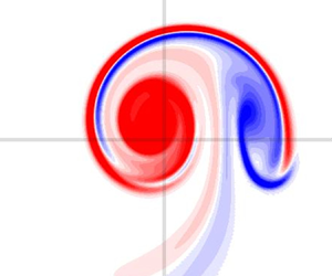
  $10^{4}$. It can be observed (see figure 3 for $\omega _{\scriptscriptstyle B}$, and 4 for ${u_{{\scriptscriptstyle H}}}$) that filaments are emitted during the early relaxation stage (see $t=4$), and then quickly dissipate ( $t=10$) while the vortex becomes quasi-steady ( $t=20$).

Figure 3. Case A at  $t=4$, $10$ and $20$: contours of ${\omega _{{\scriptscriptstyle B}}}/{\omega _{{\scriptscriptstyle B}}}_{{max}}(t)$ in plane $\varPi _\perp (t)$. Contours levels are as defined in figure 2.

Figure 4. Case A at  $t=0$, $4$,
$4$,  $10$ and $20$: contours of ${u_{{\scriptscriptstyle H}}}/{u_{{\scriptscriptstyle H}}}_{{max}}$ in plane $\varPi _\perp (t)$. Contours levels are defined in the same way as in figure 2 for ${\omega _{{\scriptscriptstyle B}}}/{\omega _{{\scriptscriptstyle B}}}_{{max}}$.
We check how the DNS solution approaches an Euler equilibrium using conditions (3.15a,b). First, we determine the translating reference frame: velocity  $U_0(t)$ is computed by the best correlation of the vorticity field between successive time steps. Second, the streamfunction $\varPsi ^{{(T)}}$ in the translating frame is computed using (3.6). From now on, we only consider streamfunction $\varPsi ^{{(T)}}$ which will be simply denoted as $\varPsi$. Figure 5(a,d,g) displays scatterplots of $u_{\scriptscriptstyle H}$ vs $\varPsi$ at several times for case A. As time increases, it is observed that the points converge to a single continuous curve, supporting the existence of the function $g$ such that $u_{\scriptscriptstyle H}=g(\varPsi )$. The second condition (3.15a,b) requires the derivative $\mathrm {d} u_{\scriptscriptstyle H} / \mathrm {d} \varPsi$, a quantity which is defined only if a steady state is reached. A procedure is proposed in Appendix A to provide an estimate value for this derivative (see formula (A4)) during the whole time evolution, that converges to the exact value when the quasi-steady state is reached. In figure 5(b,e,h), scatterplots of quantity $\varpi$ vs $\varPsi$ are found to support the existence of a function $f$ such that $\varpi =f(\varPsi )$.

Figure 5. Case A: scatterplots at times  $t=0$ (a–c), $t=2$ (d–f) and $t=20$ (g–i): (a,d,g) ${u_{{\scriptscriptstyle H}}}$ vs $\varPsi$ (the red curve is an estimate of $g(\varPsi )$ obtained via formula (A3)); (b,e,h) $\varpi$ vs $\varPsi$; (c, f,i) $\alpha \omega _{\scriptscriptstyle B}$ (black dots) and $\alpha ^2 \mathrm {d} (u_{\scriptscriptstyle H} + C)^2 / \mathrm {d} \varPsi$ (blue dots) vs $\varPsi$. Note that only grid points such that $\omega _{\scriptscriptstyle B}/\omega _{{\scriptscriptstyle B}\,max}>10^{-3}$ have been represented.
For case A, however, quantity  $\alpha \omega _{\scriptscriptstyle B}$ dominates the value $\varpi$ (see figure 5c, f,i): when the jet component is weak, quantity $\varpi$ almost equals $\alpha {\omega _{{\scriptscriptstyle B}}}$, which visually becomes a function of $\varPsi$. We present a second simulation (case B) where the jet component is initially more intense: circulation $\varGamma =1$, initial helix radius $r_{\mathrm {A}\!^{\star }}=1$, reduced pitch $L=1.5$, initial core size $a^\star =0.2$ and initial axial flow intensity ${u^\star _{\scriptscriptstyle H}}=2$. This yields $\omega _{\scriptscriptstyle B}^\star = 9.52$. The Reynolds number is set to $\mbox {Re}=10^3$. As time evolves, velocity ${u_{{\scriptscriptstyle H}}}$ converges to a function of $\varPsi$ (see figures 6a,d,g and 6b,e,h). For case B, partial quantities $\alpha {\omega _{{\scriptscriptstyle B}}}$ and $\alpha ^2 \mathrm {d} (u_{\scriptscriptstyle H} + C)^2 / \mathrm {d} \varPsi$ have same orders of magnitude (see figure 6c, f,i) so that the corresponding points remain scattered even at late times. Quantity $\varpi =\alpha {\omega _{{\scriptscriptstyle B}}} - \alpha ^2 \mathrm {d} (u_{\scriptscriptstyle H} + C)^2 / \mathrm {d} \varPsi$, however, clearly converges towards a function of $\varPsi$ (see figure 6b,e,h). This fully confirms the new finding expressed by relations (3.15a,b).

Figure 6. Same as figure 5 but for case B (see text) plotted at times  $t=0$ (a–c), $t=50$ (d–f) and $t=100$ (g–i).
Figure 7 represents the relation reached in the quasi-equilibrium state between  $\varpi$ and ${u_{{\scriptscriptstyle H}}}$. When axial vorticity dominates over axial velocity (figure 7a) there is a linear relationship between $\varpi \approx \alpha {\omega _{{\scriptscriptstyle B}}}$ and ${u_{{\scriptscriptstyle H}}}$. When both effects have comparable orders of magnitude, this relation becomes highly nonlinear (figure 7b). Finding an analytical expression for such relations remains an open issue.


4.3. Determination of the centre of the helical vortex
The above results suggest that, in order to characterize the structure of the vortex, the most convenient way is to select the point of maximum  $\varPsi$ as a centre for the vortex. When this quantity is available, one looks for the point A where $\varPsi$ reaches a maximum in the plane $\varPi _0$ (for most single helical vortices, this point is unique), and one defines the associated plane $\varPi _\perp$ in a similar way as $\varPi _\perp ^\star$ is defined from ${\mathrm {A}\!^{\star }}$ (see above in § 4.1 and figure 1). Since the field $\varPsi$ depends on $(r,\varphi )$, there is a one-to-one relation between its values in the plane $\varPi _\perp$ and in the plane $\varPi _0$. Consequently, it also reaches a maximum in the $\varPi _\perp$ plane at point A. Other properties can be also useful to locate this central point. Since $r u_r = \partial _\varphi \varPsi$ and $u_\varphi = -\alpha (r)\partial _r\varPsi$, velocity at point A is such that $u_r=u_{\varphi }=0$ and is thus tangent to a helical line, i.e. $\boldsymbol {u}(\textrm {A})={u_{{\scriptscriptstyle B}}} {\boldsymbol {e}_{\scriptscriptstyle B}}$. Furthermore, if the solution is a quasi-steady equilibrium, then relation $u_{\scriptscriptstyle H}+C=g(\varPsi )$ holds and, necessarily, velocity $u_{\scriptscriptstyle H}$ has an extremum at point A because, at point A
 \begin{equation} \partial_\varphi {u_{{\scriptscriptstyle H}}} = \frac{\mathrm{d} {u_{{\scriptscriptstyle H}}}}{\mathrm{d} \varPsi} \partial_\varphi \varPsi=0, \quad \partial_r {u_{{\scriptscriptstyle H}}} = \frac{\mathrm{d} {u_{{\scriptscriptstyle H}}}}{\mathrm{d} \varPsi} \partial_r\varPsi =0. \end{equation}
Since  $\partial _\varphi {u_{{\scriptscriptstyle H}}}=r\omega _r$ and $\partial _r {u_{{\scriptscriptstyle H}}}=-\omega _{\varphi }/\alpha$, vorticity at point A is such that $\omega _r=\omega _{\varphi }=0$ and is thus tangent to a helical line, i.e. $\boldsymbol {\omega }(\textrm {A})={\omega _{{\scriptscriptstyle B}}}{\boldsymbol {e}_{\scriptscriptstyle B}}$. The points where $\alpha \omega _{\scriptscriptstyle B}$ and ${u_{{\scriptscriptstyle H}}}$ reach an extremum generally do not coincide. Only in the particular case when $u_{\scriptscriptstyle H}=0$, quantity $\alpha \omega _{\scriptscriptstyle B}$ is also a function of $\varPsi$ and thus reaches an extremum at the same point. This is illustrated in table 1: for case A with relatively small axial flow, these radial locations differ by less than 0.1 %, while they differ by 3 % for case B because of the larger axial flow.
Table 1. Radial location of the maximum for different quantities, as measured in the DNS for cases A and B.

4.4. Quasi-equilibrium helical vortex with prescribed parameter values
The viscous quasi-equilibrium reached after a given simulation time depends on five dimensional parameters used to initiate the simulation as explained in § 4.1, namely circulation  $\varGamma$, helix radius $r_{\mathrm {A}\!^{\star }}$, helical pitch $2{\rm \pi} L$, vortex core size $a^\star$, axial flow intensity ${u^\star _{\scriptscriptstyle H}}$. The vorticity amplitude ${\omega ^\star _{\scriptscriptstyle B}}$ is a function of circulation $\varGamma$ and velocity ${u^\star _{\scriptscriptstyle H}}$. The goal is to generate a quasi-equilibrium to be used as a base flow in an instability study. Hence, we would like to prescribe the final state obtained through the DNS rather than the initial state (4.5a,b). In order to characterize the final state, we need to define five such parameters. The centre A of the vortex can be determined as explained in the previous section, yielding the helix radius $r_{A}$. The helical pitch is a fixed value $2{\rm \pi} L$ and circulation $\varGamma$ is given by
 \begin{equation} \varGamma \equiv \iint_{\varPi_0} \omega_{z} \, r\, \mathrm{d} r \,\mathrm{d} \theta. \end{equation}
The core size can be obtained through an integral in the plane  $\varPi _\perp$ associated with point A
 \begin{equation} a^{2} \equiv \frac{1}{\varGamma} \iint_{\varPi_{{\perp}}} \boldsymbol{\omega} \boldsymbol{\cdot} \boldsymbol{e}_{{\scriptscriptstyle B}_{A}} \left(\boldsymbol{x}-\boldsymbol{x}_{A} \right)^{2} d S_{{\perp}}, \end{equation}
where  $\boldsymbol {e}_{{\scriptscriptstyle B}_{A}} \equiv \boldsymbol {e}_{{\scriptscriptstyle B}}(\textrm {A})$ and $\boldsymbol {x}_{A}\equiv \boldsymbol {x}(\textrm {A})$. The last parameter is the axial velocity parameter
 \begin{equation} W_B \equiv \frac{ \alpha_{A}^2}{{\rm \pi} a^2} \iint_{\varPi_{0}} {u_{{\scriptscriptstyle H}}} \,\mathrm{d} S \quad \text{with } \alpha_{A} \equiv \alpha(r_{A}). \end{equation}
An inverse swirl number can be defined as the ratio of the axial velocity parameter  $W_B$ and the typical azimuthal velocity in the core $\varGamma /(2{\rm \pi} a)$
 \begin{equation} \bar W_B \equiv \frac{ 2{\rm \pi} a\, W_B}{ \varGamma }. \end{equation}
If the profiles are close to a thin curved Batchelor vortex (4.5a,b), the core size  $a$ is almost equal to $a^\star$ and the quantity $W_B$ is close to the amplitude of helical velocity $\alpha _{A}{u^\star _{\scriptscriptstyle H}}$. Indeed, for a thin core, $\mathrm {d} S_{\perp } \approx \alpha \,\mathrm {d} S \approx \alpha _{A}\, \mathrm {d} S$ and
 \begin{align} W_B \approx \frac{\alpha_{A}}{{\rm \pi} a^2} \iint_{\varPi_{{\perp}}} {u_{{\scriptscriptstyle H}}} \mathrm{d} S_\perp=\frac{\alpha_{A}}{{\rm \pi} a^2} {{u^\star_{\scriptscriptstyle H}} } 2 {\rm \pi}\int_{0}^{\infty} \mathrm{e}^{-(\rho/{a^\star})^{2}} \rho \,\mathrm{d} \rho =\frac{\alpha_{A}}{{\rm \pi} a^2}{u^\star_{\scriptscriptstyle H}} {\rm \pi}a^{\star2}\approx \alpha_{A} {u^\star_{\scriptscriptstyle H}}. \end{align}
Another possibility for obtaining a value for  $a$ and $W_B$ is to use a Gaussian fit of the axisymmetric component of fields ${\omega _{{\scriptscriptstyle B}}}$ and/or ${u_{{\scriptscriptstyle H}}}$.
From now on in § 4, all variables are put in dimensionless form using as characteristic dimensional length scale  $r_{{A}}$ and time scale $r^2_{{A}}/\varGamma$ of the final state. Since the dimensionless radius at point A and dimensionless circulation are equal to one, the quasi-equilibrium state depends only on two dimensionless lengths $L$ and $a$, and on the inverse swirl number $\bar W_B$. In order to simulate the dynamics of the vortex towards the quasi-equilibrium, we also need to select a value for the Reynolds number $\mbox {Re}\equiv \varGamma /(2{\rm \pi} \nu )$ and a simulation time denoted as $T_{sim}$. In the two-dimensional framework, it is known that the characteristic time necessary for the vortex to reach a quasi-equilibrium is of order $a^2\mbox {Re}^{{1}/{3}}$ with a pre-factor of order 40 (Bernoff & Lingevitch Reference Bernoff and Lingevitch1994). We here select the final simulation time $T_{sim}\sim 60a^2 \mbox {Re}^{{1}/{3}}$ and, in practice, check a posteriori that it is large enough to reach a quasi-equilibrium. For $\mbox {Re}=10^4$, for instance, we selected $T_{sim}=20, 40, 100$ for $a=0.11, 0.174$ and $0.3$, respectively.
The reduced pitch  $L$ and circulation $\varGamma$ of the initial condition are identical to those of the quasi-equilibrium we are looking for (hereafter called the final state). By contrast, initial parameters $r_{\mathrm {A}\!^{\star }}$, $a^\star$ and ${u^\star _{\scriptscriptstyle H}}$ differ from the final quantities $r_{A}=1$, $a$ and $W_B/\alpha _{{A}}$. We use an iterative procedure to determine these three unknown parameters. First, we select guess values for $a^\star$ and $r_{\mathrm {A}\!^{\star }}$, so that we link the two initial parameters ${u^\star _{\scriptscriptstyle H}}$ and ${\omega ^\star _{\scriptscriptstyle B}}$ to parameters ${a}$, $L$ and $\bar W_B$. This connection is obtained via two ‘conservation’ laws (B6) and (B12) obtained in Appendix B. They read in dimensionless form
 \begin{equation} \mathcal{H}_1(t)-\frac{2}{L}\mathcal{H}_2(t)=1,\quad \mathcal{H}_4(t) = \mathcal{H}_4(0) -\frac{2t}{L\,\mbox{Re}}, \end{equation}
where
 \begin{equation} \mathcal{H}_1 \equiv \iint_{\varPi_0} \alpha {\omega_{{\scriptscriptstyle B}}} \, \mathrm{d} S,\quad \mathcal{H}_2\equiv \iint_{\varPi_0} \alpha^4 {u_{{\scriptscriptstyle H}}} \, \mathrm{d} S~~~\mbox{and}~~~ \mathcal{H}_4 \equiv \iint_{\varPi_0} {u_{{\scriptscriptstyle H}}} \, \mathrm{d} S. \end{equation}
Let us introduce the quantities
 \begin{equation} {I}_p^\star (a^\star,r_{\mathrm{A}\!^{{\star}}} ,L) \equiv \iint_{\varPi_0} \alpha^p \exp(-(\rho/a^\star)^2) \,r\,\mathrm{d} r\,\mathrm{d}\theta, \end{equation}
with  $p$ positive integers. Such quantities depend on $L$ via the quantity $\rho$, itself depending on $r$,
$r$,  $\theta$, $r_{\mathrm {A}\!^{\star }}$ and $L$ (see figure 1). Inserting the initial condition (4.5a,b) into (4.12a,b) allows one to recast variables $\varGamma (t=0)$ and $\mathcal {H}_4(t=T_{sim})$ as
 \begin{equation} {\omega^\star_{\scriptscriptstyle B}} I_1^\star{-} \frac{2}{L}{u^\star_{\scriptscriptstyle H}} I_4^\star=1,\quad \mathcal{H}_4(T_{sim}) = {u^\star_{\scriptscriptstyle H}} I_0^\star{-} \displaystyle\frac{2T_{sim} }{ L\, \mbox{Re}}. \end{equation}
Introducing relation (4.10) leads to determination of  ${u^\star _{\scriptscriptstyle H}}$ and ${\omega ^\star _{\scriptscriptstyle B}}$
 \begin{equation} {u^\star_{\scriptscriptstyle H}} = \frac{1}{I_0^\star}\left[\frac{ \bar W_B a}{2\alpha_{A}^2 } + \displaystyle\frac{2 T_{sim}}{L\, \mbox{Re}}\right],\quad {\omega^\star_{\scriptscriptstyle B}} = \frac{1}{I_1^\star}\left(1+\frac{2}{L}{u^\star_{\scriptscriptstyle H}} I_4^\star\right). \end{equation}
 Of course, since  $a^\star$ and $r_{A}^\star$ have only been guessed at this stage, the DNS initiated by the above procedure does not lead at once to the prescribed values of $a$ and $r_{A}=1$ at $t=T_{sim}$. We have to use a standard iterative procedure to search for the proper pair $(a^\star,r_{\mathrm {A}\!^{\star }})$ leading, after a simulation time of duration $T_{sim}$, to the prescribed values $(a, 1)$.
4.5. Effect of Reynolds number
The ability to prescribe the final state parameters presented in the previous section makes it possible to use several distinct Reynolds numbers to try to achieve the same quasi-equilibrium state. Figure 8 shows the influence of  $\mbox {Re}$ on the two curves ${u_{{\scriptscriptstyle H}}}=g(\varPsi )$ and $\varpi =f(\varPsi )$ obtained numerically. The cases $\mbox {Re}=5000$ and $10^4$ cannot be visually distinguished, yet at lower Reynolds numbers (see $\mbox {Re}=1000$), the equilibrium curves shift more significantly as the value of $\varPsi _{max}$ also decreases. In the following, we always will adopt a sufficiently large Reynolds number (typically $\mbox {Re}=10^4$) to make sure that the quasi-equilibrium state obtained is $\mbox {Re}$-independent.

Figure 8. Relations (a)  ${u_{{\scriptscriptstyle H}}}=g(\varPsi )$ and (b) $\varpi =f(\varPsi )$ for quasi-equilibria obtained at different Reynolds numbers: $\mbox {Re}=500$ (red dots, $T_{sim}=4$), $\mbox {Re}=10^3$ (blue dots, $T_{sim}=4$), $\mbox {Re}=5\times 10^3$ (magenta dots, $T_{sim}=10$) and $\mbox {Re}=10^4$ (black solid line, $T_{sim}=20$). The dimensionless parameters of these states are $L=0.3$, $a=0.11$ and $\bar W_B = 0.2$.
4.6. Helical vortex cases
Using the procedure presented, we generate several base flow configurations with various values of parameters  $L$,
$L$,  $a$ and $\bar W_B$. For a helical vortex of reduced pitch $L$, curvature is given by $\kappa =1/(1+L^2)$ and torsion by $\tau =L/(1+L^2)$. As plotted in figure 9, curvature ${\kappa }$ decreases from $1$ to $0$ as $L$ increases from $0$, while torsion $\tau$ first increases from $0$ to $0.5$ (reached for $L=1$), and then slowly decreases to $0$. The asymptotic theory presented in § 5.1 uses parameter $\varepsilon \equiv a\kappa$ as a small parameter to introduce curvature effects on a straight axisymmetric vortex. A given value of $\varepsilon$ can be achieved from different pair values $(L, a)$, thus corresponding to different curvature and torsion levels. We choose five helical vortex states, the parameters of which are presented in table 2.

Figure 9. Non-dimensional curvature  $\kappa$ (solid line) and torsion $\tau$ (black dashed line) as functions of the reduced pitch $L$. Pitches $L$ and $1/L$ lead to the same value of the torsion but to different curvature levels, as illustrated for $L=0.7$ and $1/0.7\approx 1.43$.
Table 2. Parameters  $(\bar W_B, L, a)$ of the DNS cases investigated, with corresponding values of parameter $\varepsilon$, curvature $\kappa$ and torsion $\tau$.

The first three states correspond to the same value of  $\varepsilon =0.1$ but to different geometrical parameter values. State BS1 is characterized by relatively small values of the helical pitch and core size, leading to high curvature and low torsion. State BS2 is characterized by larger values of the helical pitch and core size, leading to low curvature but near-maximum torsion. State BS3 is the same as BS1 except that the inverse swirl parameter $\bar W_B$ is twice as much that of BS1 (or BS2). State BS4 is a state with a larger value $\varepsilon =0.16$ obtained through a larger core size. State BS5 is similar to BS4, yet with reversed axial flow (hence negative inverse swirl).
5. Core structure: asymptotic theory and DNS results
The asymptotic theory initially developed by Blanco-Rodríguez et al. (Reference Blanco-Rodríguez, Le Dizès, Selçuk, Delbende and Rossi2015) considers a straight Batchelor vortex as reference state, which is assumed to be strained via local and global effects. We start again this section using dimensional variables and suppose that there exists a frame of reference in which the helical vortex is steady. In that frame, the helical vortex is located around a centre line  $\boldsymbol {x}_0 (\theta _s) = r_{A} \boldsymbol {e}_r(\theta _s) + {L} \theta _s \boldsymbol {e}_z$ where $\theta _s$ is a continuous parameter, with associated tangent vector
 \begin{equation} \boldsymbol{e}_b \equiv\boldsymbol{e}_{{\scriptscriptstyle B}_{A}} = \alpha_{A}\left[ \frac{r_{A}}{L} \boldsymbol{e}_{\theta}(\theta_s) + \boldsymbol{e}_z \right]. \end{equation}
For a helical vortex filament, the distribution around the centreline in the plane  $\varPi _{\perp }(\textrm {A})$ is characterized by a circulation $\varGamma$ and a core size $a$. At a given point on a helical vortex, local effects are curvature and torsion, and global ones are due to the remote vorticity of nearby helix turns. Under the limitation of small core size $a$ with respect to $r_{A}$ and $L$, the vortex is close to a straight cylinder, with its local cylindrical basis $(\boldsymbol {e}_{\rho }, \boldsymbol {e}_{\psi },\boldsymbol {e}_b)$. Curvature effects are introduced as small amplitude perturbations to the reference axisymmetric state via a small self-strain parameter
 \begin{equation} \varepsilon=\alpha_{A}^2\frac{r_{A}}{L}\frac{a}{L}=\kappa a \ll 1, \end{equation}
which can then be used to expand the velocity field in power series. The theory is valid is the limit of small core sizes ( $a\ll r_{A}$ and $a\ll L$), which implies $\varepsilon \ll 1$. It has been shown in Callegari & Ting (Reference Callegari and Ting1978) and Blanco-Rodríguez & Le Dizès (Reference Blanco-Rodríguez and Le Dizès2016, Reference Blanco-Rodríguez and Le Dizès2017) that the dominant deformation stems from local curvature, and sets in as a dipolar first-order term in $\varepsilon$. Local torsion and remote vorticity effects only appear at second order. We focus here on first-order effects and characterize how local curvature deforms the vortex core.
Since the reference state is a straight Batchelor vortex, we adopt, from now on in this section, the core size  $a$ as characteristic size and $\varGamma /(2{\rm \pi} a)$ as characteristic velocity, and denote dimensionless quantities with a bar, for instance $\bar \rho =\rho /a$ stands for the non-dimensional radial distance to point A in the plane $\varPi _\perp$. We use cylindrical coordinates $(\bar \rho,\psi,b)$, where $b$ denotes the component parallel to the vortex axis. As mentioned above, the velocity field $\bar {\boldsymbol {u}}=(\bar u_{\rho },\bar u_{\psi },\bar u_b)$ can be expanded in power series in $\varepsilon$
 \begin{equation} \bar{\boldsymbol{u}}(\bar\rho,\psi)= (\varepsilon \bar u_{\rho}^{(1)}+\cdots)\;\boldsymbol{e}_{\rho} + (\bar u_{\psi}^{(0)} + \varepsilon \bar u_{\psi}^{(1)} + \cdots)\;\boldsymbol{e}_{\psi} + (\bar u_{b}^{(0)} + \varepsilon u_{b}^{(1)}+\cdots)\;\boldsymbol{e}_b , \end{equation}
with a similar expansion for vorticity.
5.1. Asymptotic expansion
The leading-order term  $\bar {\boldsymbol {u}}^{(0)}$ is assumed to be a Batchelor vortex. Indeed, this vortex model is known to be a self-similar attracting viscous solution for two-dimensional vortices with axial flow. Such a profile is also found experimentally and numerically in the core of helical vortices (Ali & Abid Reference Ali and Abid2014; Selçuk et al. Reference Selçuk, Delbende and Rossi2017; Okulov et al. Reference Okulov, Kabardin, Mikkelsen, Naumov and Sørensen2019; Shtork et al. Reference Shtork, Gesheva, Kuibin, Okulov and Alekseenko2020). This means that the velocity distribution in the plane $\varPi _{\perp }$ is
 \begin{equation} \bar u_{\rho}^{(0)} = 0,\quad \bar u_{\psi}^{(0)} = \frac{1- \exp(-\bar\rho^2)}{\bar\rho},\quad \bar u_{b}^{(0)} = \bar W_0 \exp(-\bar\rho^2) + \bar W_{00} . \end{equation}
The parameter  $\bar W_0$ indicates the jet strength in the axial direction and the parameter $\bar W_{00}$ is a correction at leading order deduced from the background velocity outside the vortex. Based on these velocity fields, the vorticity field at zeroth order in $\varepsilon$ is
 \begin{equation} \bar{\boldsymbol{\omega}}^{(0)}= \bar{\omega_{{\scriptscriptstyle B}}}^{(0)} \boldsymbol{e}_b + \bar\omega_{\psi}^{(0)} \boldsymbol{e}_\psi, \end{equation}
with
 \begin{equation} \bar{\omega_{{\scriptscriptstyle B}}}^{(0)} = 2 \exp{(- \bar\rho^2)},\quad \bar\omega_{\psi}^{(0)} = 2 \bar W_0 \bar\rho \exp{(- \bar\rho^2)}. \end{equation}
For any point M in plane  $\varPi _\perp (\textrm {A})$ except A itself, the velocity component $u_{\scriptscriptstyle B}$ along direction $\boldsymbol {e}_{\scriptscriptstyle B}(\textrm {M})$ is different from the velocity component $u_b$ along the direction $\boldsymbol {e}_b \equiv \boldsymbol {e}_{\scriptscriptstyle B}(\textrm {A})$ orthogonal to the plane. Quantity $u_{\scriptscriptstyle B}/\alpha$ is given by
 \begin{equation} \frac{u_{\scriptscriptstyle B}}{\alpha}= \frac{u_\rho}{\alpha} \;\boldsymbol{e}_{\rho} \boldsymbol{\cdot} \boldsymbol{e}_{\scriptscriptstyle B} + \frac{u_\psi}{\alpha} \;\boldsymbol{e}_{\psi} \boldsymbol{\cdot} \boldsymbol{e}_{\scriptscriptstyle B} + \frac{u_b}{\alpha} \;\boldsymbol{e}_{b} \boldsymbol{\cdot} \boldsymbol{e}_{\scriptscriptstyle B}, \end{equation}
where  $\alpha \equiv \alpha (\textrm {M})$. Using relations (deduced from relations (C3)–(C11) in Appendix C)
 \begin{equation} \boldsymbol{e}_\rho \boldsymbol{\cdot} \boldsymbol{e}_{\scriptscriptstyle B} = 0,\quad \boldsymbol{e}_{\psi}\boldsymbol{\cdot} \boldsymbol{e}_{\scriptscriptstyle B} = \alpha \alpha_{A} \frac{\rho}{L},\quad \boldsymbol{e}_b \boldsymbol{\cdot} \boldsymbol{e}_{\scriptscriptstyle B} = \alpha \alpha_{A}\left(1 + \frac { r^2_{A}}{L^2} -\frac{r_{A}}{L}\frac{\rho}{L} \cos \psi \right), \end{equation}
one obtains, at zeroth order in  $\varepsilon$
 \begin{align} \frac{\bar u_{\scriptscriptstyle B}^{(0)}}{\alpha} = \frac{\bar u^{(0)}_b(\bar\rho)}{\alpha_{A}} + {\bar u^{(0)}_\psi(\bar\rho)}{\alpha_{A}}\frac{\bar \rho}{\bar L} = \frac{1}{\alpha_{A}}[\bar W_0 \exp{(- \bar\rho^2)} +\bar W_{00}]+\frac{\alpha_{A}}{\bar L}[1- \exp{(- \bar\rho^2)}]. \end{align}
Quantity  $\bar W_0$ is, by construction, given by $\bar W_0 = \bar u^{(0)}_b(0) -\bar u^{(0)}_b(\infty )$. Using relation (5.9) twice at $\bar \rho =0$ and at the limit $\bar \rho \to \infty$, one deduces, at zeroth order in $\varepsilon$
 \begin{equation} \bar W_0 = \alpha_{A}\left(\frac{\bar u^{(0)}_{\scriptscriptstyle B}(0)}{\alpha_{A}}-\frac{\bar u^{(0)}_{\scriptscriptstyle B}(\infty)}{\alpha}\right) + \frac{\alpha_{A}^2}{\bar L} = \alpha_{A}\bar u^{(0)}_{\scriptscriptstyle H}(0) + \frac{\alpha_{A}^2}{\bar L}. \end{equation}
Quantity  $\bar W_{00}$ can be obtained by matching the value reached by $\bar u_{\scriptscriptstyle B}^{(0)} / \alpha$ outside the vortex to the constant introduced in (3.10)
 \begin{equation} \bar C = \frac{2{\rm \pi} a C}{\varGamma} = \frac{1}{\bar L}+\bar U_z^{\infty{(T)}}. \end{equation}
As  $\bar \rho \to \infty$, expression (5.9) tends to $\bar W_{00}/\alpha _{A}+\alpha _{A}/\bar L$. The matching eventually yields
 \begin{equation} \bar W_{00} = \alpha_{A}\left(\bar C - \frac{\alpha_{A}}{\bar L}\right) = \alpha_{A}\bar U_z^{\infty{(T)}} + \frac{\alpha_{A}(1 -\alpha_{A})}{\bar L}. \end{equation}
In Blanco-Rodríguez et al. (Reference Blanco-Rodríguez, Le Dizès, Selçuk, Delbende and Rossi2015), the simplified expression  $\bar W_{00} \approx \alpha _A U_z^{\infty {(T)}}$ was used. Expression (5.12) shows a better agreement with the numerical results (see § 5.2).
The two constants  $\bar W_0$ and $\bar W_{00}$ can thus be related to the parameter values of the base helical vortex using (5.10) and (5.12) with $\bar U_z^{\infty {{(T)}}}=-\bar U_0 = \bar \varOmega _0\bar L$
 \begin{equation} \bar W_0 \approx \bar W_B + \frac{\alpha_{A}^2}{\bar L},\quad \bar W_{00} =\alpha_{A} \bar\varOmega_0\bar L + \frac{\alpha_{A}(1-\alpha_{A})}{\bar L} . \end{equation}
The evaluation of  $\bar W_{00}$ requires the knowledge of $\bar \varOmega _0$. Although this latter quantity could be computed theoretically (Okulov Reference Okulov2004) as done by Brynjell-Rahkola & Henningson (Reference Brynjell-Rahkola and Henningson2020), we use here the value deduced from the DNS results.
Going now to order  $\varepsilon$, the perturbation is purely dipolar (Blanco-Rodríguez et al. Reference Blanco-Rodríguez, Le Dizès, Selçuk, Delbende and Rossi2015)
 \begin{gather} \bar u_{\rho}^{(1)} ={-} \frac{\bar\varPsi^{(1)}}{\bar\rho} \sin \psi,\quad \bar u_{\psi}^{(1)}= \left[ \bar\rho\bar u^{(0)}_\psi -\frac{\mathrm{d} \bar\varPsi^{(1)}}{\mathrm{d} \bar\rho} \right] \cos \psi, \end{gather}
 \begin{gather} \bar u_{b}^{(1)} = \left[\bar\rho\bar u^{(0)}_b - \frac{1}{\bar u^{(0)}_\psi}\frac{\mathrm{d}\bar u^{(0)}_b}{\mathrm{d}\bar\rho}\bar\varPsi^{(1)} \right] \cos \psi, \end{gather}
where the first-order streamfunction perturbation  $\bar \varPsi ^{(1)}(\bar \rho )$ satisfies
 \begin{equation} \bar\varPsi^{(1)}= \bar\varPsi^{(1)}_0 + \bar W^2_0 \bar\varPsi^{(1)}_1 + \bar W_{00} \bar W_0 \bar\varPsi^{(1)}_2. \end{equation}
The three contributions  $\bar \varPsi ^{(1)}_0$, $\bar \varPsi ^{(1)}_1$ and $\bar \varPsi ^{(1)}_2$ are solutions of
 \begin{equation} \mathcal{L} \bar\varPsi^{(1)}_0 = \bar K_0,\quad \mathcal{L}\bar\varPsi^{(1)}_1 = \bar K_1,\quad \mathcal{L} \bar\varPsi^{(1)}_2 =\bar K_2, \end{equation}
where the linear operator  $\mathcal {L} (\bullet )$ is defined as
 \begin{equation} \mathcal{L} ({\bullet}) \equiv \frac{ \partial^2 ({\bullet}) }{ \partial \bar\rho^2}+ \frac{1 }{\bar\rho} \frac{ \partial ({\bullet}) }{ \partial \bar\rho} - \left(\frac{1 }{\bar\rho^2} + H_0(\bar\rho)\right) ({\bullet}) \end{equation}
and
 \begin{equation} \left. \begin{aligned} \bar H_0(\bar\rho) & \equiv \frac{1 }{\bar u_{\psi}^{(0)} } \frac{ \mathrm{d} \bar{\omega_{{\scriptscriptstyle B}}}^{(0)} }{ \mathrm{d} \bar\rho}= \frac{-4\bar\rho^2}{\exp{(\bar\rho^2)} -1},\\ \bar K_0(\bar\rho) & \equiv 2 \bar\rho\bar\omega^{(0)}_b +\bar u_{\psi}^{(0)} = \frac{1- \exp{(- \bar\rho^2)}}{\bar\rho} + 4 \bar\rho \exp{(- \bar\rho^2)} ,\\ \bar K_1(\bar\rho) & \equiv{-} \frac{4 \bar\rho^3 }{\exp{( \bar\rho^2)} -1 } \exp{(- \bar\rho^2)},\quad \bar K_2(\bar\rho) \equiv{-}\frac{4 \bar\rho^3 }{\exp{( \bar\rho^2)} -1 } . \end{aligned} \right\} \end{equation}
The boundary conditions at  $\bar \rho =0$ are
 \begin{equation} \bar\varPsi^{(1)}_{i}(0)=0,\quad \frac{ \partial \bar\varPsi^{(1)}_{i} }{ \partial \bar\rho}(0)=0,\quad i=0, 1, 2. \end{equation}
We hence compute the first-order streamfunction perturbation  $\bar \varPsi ^{(1)}$ numerically. For large $\bar \rho$, $\bar \varPsi ^{(1)}(\rho )$ expands as (Fukumoto & Miyazaki Reference Fukumoto and Miyazaki1991)
 \begin{equation} \bar\varPsi^{(1)}(\bar\rho) \sim \frac{1}{2}\bar\rho\log \bar\rho + \bar\rho \bar A + O\left(\frac{1}{\bar\rho}\right), \end{equation}
where, for the Batchelor vortex profile,  $\bar A$ reads as
 \begin{equation} \bar A = \frac{1}{4}[1-\bar W_0(\bar W_0+4 \bar W_{00})+ \gamma - \log 2],\quad \gamma\approx0.577. \end{equation}
This formula corrects the typo  $2\bar W_{00}$ in (3.12) of Blanco-Rodríguez et al. (Reference Blanco-Rodríguez, Le Dizès, Selçuk, Delbende and Rossi2015).
5.2. Comparison with DNS results
Quasi-equilibrium states listed in table 2 are obtained as final states of simulations through the procedure explained in § 4.4. Figure 10(a) (respectively figure 10b) shows the axial vorticity in the plane  $\varPi _\perp$ for BS1 (respectively BS2). In addition, the internal structure can be compared with the results obtained by the asymptotic theory presented in § 5.1. To do so, one needs not only to rewrite the DNS results in the reference frame and in the basis used in the theory, but also to use the same non-dimensionalization process. More precisely, this means:
(i) adopting the frame ${(T)}$ translating at velocity $U_0 \boldsymbol {e}_z$ with the vortex. This amounts to transforming two of the velocity components: $u_{\scriptscriptstyle B} \longrightarrow u_{\scriptscriptstyle B}-\alpha U_0$ and $u_\varphi \longrightarrow u_\varphi +\alpha U_0 r/L$;
(ii) projecting the velocity field onto the plane
$\varPi _\perp (\textrm {A})$ in order to get in-plane components $(u_\rho, u_\psi )$ and deduce out-of-plane component $u_b$, as explained in Appendix C;(iii) performing an azimuthal decomposition in
$\varPi _\perp (\textrm {A})$ of such components using
(5.23)where\begin{equation} u_{\rho,\psi,b}^{(m)}(\rho_{i})=\frac{1}{N_{\psi}} \sum_{j=1}^{N_{\psi}} u_{\rho,\psi,b}(\rho_{i}, \psi_{j}) \mathrm{e}^{-\mathrm{i} m \psi_{j}}\quad (i=1,\ldots,N_\rho), \end{equation}$(\rho _{i}, \psi _{j})$ are the locations of $N_\rho \times N_\psi$ nodes of a polar mesh in plane $\varPi _\perp$; and(iv) making the various quantities dimensionless using the reference scales
$a_0$ and $2{\rm \pi} a_0^2/\varGamma$ as for the theory.


Based on the above procedure, the parameters presented in table 2 correspond to the values of effective core size  $a_0$, inverse swirl $\bar W_0$ and constant $\bar W_{00}$ reported in table 3. Each case has been analysed, showing the adequacy of the asymptotic theory up to relatively large values of $\varepsilon$. Comparisons between asymptotic theory and DNS of helical vortices are shown in figures 11 and 12 for BS1 ( $\varepsilon =0.1$) and BS5 ( $\varepsilon =0.16$), respectively. In each graph, the $m=0$ and $m=1$ contributions to $(u_\rho ^{(m)},u_\psi ^{(m)},u_b^{(m)})$ are plotted. Excellent agreement is found for the axisymmetric part. A fairly small mismatch subsists for the components of the $m=1$ contribution.

Figure 10. (a) Contours of  $\omega _{\scriptscriptstyle B}$ in plane $\varPi _\perp$ for the quasi-equilibrium state BS1. (b) Same for BS2, with the same spatial range represented. Contour levels are as in figure 2. The Reynolds number is $\mbox {Re} = 10^4$, and the simulation time $T_{sim}=20$ (respectively 100) for BS1 (respectively BS2).

Figure 11. Case BS1: radial distributions of velocity components  $(\bar u_\rho ^{(m)},\bar u_\psi ^{(m)},\bar u_b^{(m)})$ for $m=0$ (a–c) and $m=1$ (d–f). Blue solid line: DNS results; red dashed line: theory.

Figure 12. Same as figure 11 for case BS5.
Table 3. For the different helical vortex states under study: case parameters  $a$ and $\bar W_B$; effective core size $a_0$ and inverse swirl $\bar W_{0}$ obtained by DNS; values of $\bar W_B+\alpha _A^2/\bar L$ and $\bar W_{00}$ obtained through (5.13a,b).

6. Discussion and conclusion
In this paper, we have shown that, when a moderate axial flow is present in a helical vortex, a quasi-equilibrium can be reached. In a suitable translating frame (T), such a solution can be related to a broader family of equilibria of inviscid flows characterized by a helical symmetry of pitch  $2{\rm \pi} L$. We have first exhibited the constraints (3.15a,b) of such equilibria, which involve the velocity and vorticity components $u_{\scriptscriptstyle B}^{(T)}$ and $\omega _{\scriptscriptstyle B}$: introducing a streamfunction $\varPsi ^{(T)}$ defined by (2.1), there exist two functions $f$ and $g$ such that $\varpi =f(\varPsi ^{(T)})$ and $u_{\scriptscriptstyle B}^{(T)}/\alpha =g(\varPsi ^{(T)})$, where $\varpi$ is defined in (3.14). Such relationships, which extend formulae known for vortex rings, are indeed reached in time through DNS when a single helical vortex with an axial flow relaxes towards quasi-equilibrium. We also describe a numerical procedure aimed at computing vortex solutions with all parameters prescribed, namely circulation, helix radius, helical pitch, vortex core size and swirl level. The procedure is first used to show that such quasi-equilibria do not depend on the Reynolds number used to generate them, if sufficiently large. More generally they can be used as basic flow profiles for the purpose of instability studies, and several helical vortex states are described (see parameters in table 2). Finally, when the core size is reasonably small with respect to the helical pitch and the curvature radius, the asymptotic theory is shown to adequately describe the structure of the DNS velocity field. At zeroth order (local axisymmetric contribution), the flow is found to be very close to a straight Batchelor vortex flow profile, a property that is used to compute the dipolar correction at first order due to the curvature of the vortex; excellent agreement is found between numerics and asymptotic theory.
The procedure used above relies on the assumption that the initial condition rapidly relaxes towards a quasi-equilibrium. However, when the axial flow becomes large, such an equilibrium ceases to exist because the swirling motion can no longer counter-balance the centrifugal forces generated by axial velocity in the curved vortex. In terms of vorticity, negative helical vorticity emerges and may persist over large evolution times. We can define a threshold value  $\bar W_B^{c}$ above which negative vorticity is still present at $t=T_{sim}$ (here $T_{sim}=4$ at $\mbox {Re}=10^3$). In figure 13, we present the evolution of this threshold $\bar W_B^{c}$ as a function of the reduced pitch at fixed core size $a=0.11$. For given $L$ and $\bar W_B< \bar W_B^{c}(L)$, the simulation converges towards a quasi-equilibrium state as shown in figure 14(a–d). For $\bar W_B> \bar W_B^{c}(L)$, the system does not rapidly reach such an equilibrium (figure 14e–h). A dipolar structure can even emerge, as illustrated in figure 15. This phenomenon is similar to what is observed in vortex rings by Cheng, Lou & Lim (Reference Cheng, Lou and Lim2010) when the axial flow becomes significant. Note also that the threshold value shown in figure 13 pinpoints the existence of an equilibrium up to relatively large values of $\bar W_B$. However, we suspect this helical equilibrium state to be itself unstable with respect to the swirling jet instability that occurs as soon as $\bar W_B>0.7$ for a straight Batchelor vortex (Lessen et al. Reference Lessen, Singh and Paillet1974; Mayer & Powell Reference Mayer and Powell1992). In our simulations, enforcing the helical symmetry filters out such instabilities.

Figure 13. Axial flow critical level  $\bar W_B^{c}(L)$ above which the initial condition does not relax towards a quasi-steady equilibrium. Simulations with $a=0.11$, $\mbox {Re}=10^3$ and $T_{sim}=4$.

Figure 14. Time evolution of a helical vortex at  $L=0.3$, $a=0.11$ and $\mbox {Re}=10^3$ with axial flow (a–d) $\bar W_B=1.8$ (below the critical threshold) and (e–h) $\bar W_B=1.9$ (above it). Contours of $\omega _{b}/\omega _{b\,max}$ in plane $\varPi _\perp (t)$. Contour levels are regularly spaced in the range $[-1/e, 1/e]$ (from blue to red).

Figure 15. Time evolution of a helical vortex at  $L=1.43$, $a=0.3$ and $\mbox {Re}=10^3$ with axial flow $\bar W_B=4.0$ (above the threshold). Contours are as in figure 14.
In the present paper, the method and the data are presented in the case of a single helical vortex. This could be easily extended to an arbitrary number of vortices with the same helical pitch in a quasi-equilibrium arrangement. These states are of great significance for the instability studies of vortices with a helical shape, e.g. in the wake of wind turbines, marine propellers, helicopter rotors $\ldots\,$. Let us stress the importance of monitoring the axial velocity in such vortices, since curvature and elliptic short-wave instabilities crucially depend on the swirl parameter (Hattori & Fukumoto Reference Hattori and Fukumoto2014). In this perspective, the present work provides a procedure to generate basic states with prescribed values of the numerous parameters characterizing the helical vortex, namely circulation, helix radius, helical pitch, vortex core size and swirl level.
Acknowledgements
The authors would like to thank Y. Hattori for fruitful discussions.
Declaration of interests
The authors report no conflict of interest.
Appendix A. Estimating quantity $\mathrm {d}{u_{{\scriptscriptstyle H}}}/\mathrm {d}\varPsi$

The second condition of (3.15a,b) requires the derivative  $\mathrm {d} u_{\scriptscriptstyle H} / \mathrm {d} \varPsi$. This quantity is a priori defined only if a steady state is reached. The following procedure, however, allows us to estimate this quantity during the whole time evolution, based on averages and least square interpolation. More specifically, we discretize the $\varPsi$-axis in $N_\varPsi$ intervals of length $\Delta \varPsi$ between the minimum and the maximum value of $\varPsi$. In each interval $[\varPsi _{i}-{\Delta \varPsi }/2, \varPsi _{i}+{\Delta \varPsi }/2]$, there is a certain number $K_i$ of points $(\varPsi ^{(k)},u_{\scriptscriptstyle H}^{(k)})$ indexed by $k$. The mean value $\alpha _i$ of $u_{\scriptscriptstyle H}^{(k)}$ and the estimate $\beta _i$ of $\mathrm {d} u_{\scriptscriptstyle H} /\mathrm {d} \varPsi$ at point $\varPsi _i$ are such that
 $$\begin{gather} K_i \alpha_i+ \beta_i \sum_k (\varPsi^{(k)} -\varPsi_{i}) = \sum_k u_{\scriptscriptstyle H}^{(k)}, \end{gather}$$
 $$\begin{gather}\alpha_i \sum_k (\varPsi^{(k)} -\varPsi_{i}) +\beta_i \sum_k (\varPsi^{(k)} -\varPsi_{i})^2 =\sum_k [u_{\scriptscriptstyle H}^{(k)}(\varPsi^{(k)} -\varPsi_{i}) ], \end{gather}$$
where it has been assumed that  $u_{\scriptscriptstyle H}^{(k)}$ can be estimated with the linear interpolation
 \begin{equation} u_{\scriptscriptstyle H}^{(k)} = \alpha_i + \beta_i (\varPsi^{(k)}-\varPsi_{i}). \end{equation}
Quantities  $\mathrm {d} u_{\scriptscriptstyle H} / \mathrm {d} \varPsi$ are computed using a linear interpolation along the variable $\varPsi$ as follows:
 \begin{equation} \frac{\mathrm{d}
u_{\scriptscriptstyle H} }{\mathrm{d}
\varPsi_T}(\varPsi^{(k)})= \beta_i + \left\{
\begin{array}{@{}c@{}} {\beta_{i+1}-\beta_i} \\
{\beta_i-\beta_{i-1}} \end{array} \right\}
\frac{\varPsi^{(k)}-\varPsi_{i} }{\Delta \varPsi} \quad
\left\{ \begin{array}{@{}c@{}} \text{if}\
\varPsi^{(k)}>\varPsi_{i} \\ \text{if}\
\varPsi^{(k)}<\varPsi_{i} \end{array} \right. .
\end{equation}
\begin{equation} \frac{\mathrm{d}
u_{\scriptscriptstyle H} }{\mathrm{d}
\varPsi_T}(\varPsi^{(k)})= \beta_i + \left\{
\begin{array}{@{}c@{}} {\beta_{i+1}-\beta_i} \\
{\beta_i-\beta_{i-1}} \end{array} \right\}
\frac{\varPsi^{(k)}-\varPsi_{i} }{\Delta \varPsi} \quad
\left\{ \begin{array}{@{}c@{}} \text{if}\
\varPsi^{(k)}>\varPsi_{i} \\ \text{if}\
\varPsi^{(k)}<\varPsi_{i} \end{array} \right. .
\end{equation}
For the first and the last half-intervals, one uses an extrapolation from the neighbouring half-interval.
Appendix B. Relations for some global quantities in viscous helical flows
In this appendix, quantities are dimensional. For a viscous flow of specific volume  $\upsilon$ periodic along $z$ of period $2 {\rm \pi}L$ and characterized by a compact vorticity field, the circulation $\varGamma$ and the axial momentum per unit length $\mathcal {P}_z$ given by
 \begin{align} \varGamma = \iint_{\varPi_0} \omega_{z} \, r \,\mathrm{d} r \,\mathrm{d} \theta,\quad \mathcal{P}_z= \frac{1}{2 {\rm \pi}L} \left(\frac{1}{2\upsilon}\,\iiint_V\boldsymbol{x}\times\boldsymbol{\omega}\,\mathrm{d} V \right)\boldsymbol{\cdot}\boldsymbol{e}_z = \frac{1}{4 {\rm \pi}L \upsilon}\,\iiint_V r {\omega}_{\theta}\,\mathrm{d} V, \end{align}
are two global viscous invariants. In (B1a,b),  $\varPi _{0}$ denotes the plane $z=0$ and $V$ the volume defined by $z \in [-{\rm \pi} L, {\rm \pi}L]$. For such periodic flows, the axial angular momentum per unit length
 \begin{equation} \mathcal{L}_{z} ={-} \frac{1}{4 {\rm \pi}L\upsilon} \iiint_{V} \boldsymbol{x}^2{\omega}_z\,\mathrm{d} V \end{equation}
is not an invariant but evolves according to
 \begin{equation} \displaystyle\frac{\mathrm{d}\mathcal{L}_{z}}{\textrm{d}t}={-} 2 \mu \varGamma , \end{equation}
where  $\mu \equiv \nu /\upsilon$.
These conservation laws applied to viscous helical flows (Selçuk et al. Reference Selçuk, Delbende and Rossi2017) provide relations between the following unsteady quantities:
 \begin{align} \mathcal{H}_1 \equiv \iint_{\varPi_0} \alpha {\omega_{{\scriptscriptstyle B}}} \, \mathrm{d} S,\quad \mathcal{H}_2 \equiv \iint_{\varPi_0} \alpha^4 {u_{{\scriptscriptstyle H}}} \, \mathrm{d} S,\quad \mathcal{H}_3 \equiv \iint_{\varPi_0} r^2 \alpha {\omega_{{\scriptscriptstyle B}}} \,\mathrm{d} S ,\quad \mathcal{H}_4 \equiv \iint_{\varPi_0} {u_{{\scriptscriptstyle H}}} \, \mathrm{d} S. \end{align}
Since  $\omega _{z} = \alpha ({\omega _{{\scriptscriptstyle B}}} - {r} \omega _{\varphi }/L)$ for helical flows, the conservation circulation $\varGamma$ yields
 \begin{equation} \varGamma = \iint_{\varPi_0} \alpha {\omega_{{\scriptscriptstyle B}}} \, \mathrm{d} S + \iint_{\varPi_0} \frac{\alpha^2 r}{L} \frac{\partial {u_{{\scriptscriptstyle H}}} }{\partial r} \, \mathrm{d} S. \end{equation}
Integrating by parts the last integral leads to
 \begin{equation} \varGamma = \mathcal{H}_1(t) -\frac{2}{L}\mathcal{H}_2(t) . \end{equation}
Similarly, the conservation of axial momentum per unit length  $\mathcal {P}_z$, implies for helical flows that
 \begin{equation} \mathcal{P}_{z} = \frac{1}{4 {\rm \pi}L\upsilon} \int^{ {\rm \pi}L}_{-{\rm \pi} L} \left[\iint_{\varPi_0} r \omega_{\theta} \, r \,\mathrm{d} r \,\mathrm{d} \theta\right] \,\mathrm{d} z =\frac{1}{2\upsilon } \iint_{\varPi_0} r^2 \omega_{\theta} \, \mathrm{d} r \,\mathrm{d} \theta. \end{equation}
Introducing  $\omega _{\theta } = \alpha (\omega _{\varphi }+ ({r}/{L}) {\omega _{{\scriptscriptstyle B}}})$ and integrating by parts, yields
 \begin{equation} \mathcal{P}_{z}\upsilon= \frac{1}{2 L } \mathcal{H}_3(t)+ \mathcal{H}_2(t). \end{equation}
Finally, helical symmetry imposes
 \begin{equation} \iiint_{V} \boldsymbol{x}^2{\omega}_z\,\mathrm{d} V = \iiint_{V} (z^2 + r^2) \omega_z\, \mathrm{d} V = \frac{2 \varGamma ({\rm \pi} L)^3}{3 } + 2 {\rm \pi}L \iint_{\varPi_0} r^2{\omega}_z\, \mathrm{d} S. \end{equation}
Upon introducing  $\omega _{z} = \alpha ({\omega _{{\scriptscriptstyle B}}} - {r} \omega _{\varphi }/L)$, one gets
 \begin{align} \iint_{\varPi_0} r^2{\omega}_z\, \mathrm{d} S\, & = \iint_{\varPi_0} \alpha r^2{\omega}_B\, \mathrm{d} S + \iint_{\varPi_0} \frac{ \alpha^2 r^3}{L} \frac{\partial {u_{{\scriptscriptstyle H}}} }{\partial r}\, \mathrm{d} S\, \nonumber\\ & = \mathcal{H}_3(t)+ \iint_{\varPi_0} rL (1-\alpha^2) \frac{\partial {u_{{\scriptscriptstyle H}}} }{\partial r}\, \mathrm{d} S. \end{align}
Integrating by parts the last integral yields
 \begin{equation} \mathcal{L}_{z}(t) ={-} \frac{1}{4 {\rm \pi}L\upsilon} \iiint_{V} \boldsymbol{x}^2{\omega}_z\,\mathrm{d} V={-} \frac{ \varGamma ({\rm \pi} L)^2}{6\upsilon } - L \mathcal{P}_{z} + \frac{L}{\upsilon} \mathcal{H}_4(t). \end{equation}
Since circulation  $\varGamma$ and axial momentum per unit length $\mathcal {P}_z$ are global viscous invariants for a compact vorticity field and that the axial angular momentum per unit length $\mathcal {L}_z(t)$ evolves according to (B3), one gets
 \begin{equation} \frac{\mathrm{d} \mathcal{H}_4}{\mathrm{d} t}={-} \frac{2 \varGamma}{L} \nu \quad \text{or equivalently}\quad \mathcal{H}_4(t) = \mathcal{H}_4(0) - \frac{2 \varGamma}{L} \nu t. \end{equation}
Appendix C. Projection of the velocity field on the $\varPi _\perp$ plane

Point A denotes the vortex centre, with the associated Serret–Frenet basis  $(\boldsymbol {e}_{r_{{{A}}}}, \boldsymbol {e}_{\varphi _{{{A}}}}, \boldsymbol {e}_{{\scriptscriptstyle B}_{{A}}})$ such that
 $$\begin{gather} \boldsymbol{e}_{\varphi_{{{A}}}}(r_{A}, \theta_{A}) =\alpha_{A}\left(\boldsymbol{e}_{\theta_{{{A}}}} -\frac{r_{A}}{L} \boldsymbol{e}_{z}\right) , \end{gather}$$
 $$\begin{gather}\boldsymbol{e}_{{\scriptscriptstyle B}_{{A}}}(r_{A}, \theta_{A}) =\alpha_{A}\left( \frac{r_{A}}{L}\boldsymbol{e}_{\theta_{{{A}}}} + \boldsymbol{e}_{z} \right) , \end{gather}$$
where  $\alpha _{A} = (1+r_{A}^2 / L^2)^{-1/2}$ (see figure 1 for a similar geometry). The plane $\varPi _\perp$ is spanned by the Cartesian basis $(\boldsymbol {e}_{r_{{{A}}}},\boldsymbol {e}_{\varphi _{{{A}}}})$, with which a local polar basis $(\boldsymbol {e}_{\rho }, \boldsymbol {e}_{\psi })$ is associated
 $$\begin{gather} \boldsymbol{e}_{\rho} =\cos \psi\, \boldsymbol{e}_{r_{{{A}}}} + \sin \psi \;\boldsymbol{e}_{\varphi_{{{A}}}}, \end{gather}$$
 $$\begin{gather}\boldsymbol{e}_{\psi} ={-}\sin \psi \boldsymbol{e}_{r_{{{A}}}} + \cos \psi \, \boldsymbol{e}_{\varphi_{{{A}}}}, \end{gather}$$
and a normal vector to the plane is  $\boldsymbol {e}_b\equiv \boldsymbol {e}_{{\scriptscriptstyle B}_{{A}}}$. The velocity field at any point M $_0$ in plane $\varPi _0$ is given by
 \begin{equation} \boldsymbol{u} (\text{M}_0) = u_r(\text{M}_0) \boldsymbol{e}_{r}(\text{M}_0) + u_\varphi(\text{M}_0) \boldsymbol{e}_{\varphi}(\text{M}_0) + u_{\scriptscriptstyle B}(\text{M}_0) \boldsymbol{e}_{\scriptscriptstyle B}(\text{M}_0). \end{equation}
In order to express the velocity field in plane  $\varPi ^\perp$ using the basis $(\boldsymbol {e}_{r_{{{A}}}},\boldsymbol {e}_{\varphi _{{{A}}}},\boldsymbol {e}_{{\scriptscriptstyle B}_{{A}}})$, one first determines the intersection M between the helical line passing through M $_0$ and the plane $\varPi _\perp$, where the velocity is
 \begin{equation} \boldsymbol{u} (\text{M}) = u_{\rho}(\text{M})\boldsymbol{e}_{\rho}(\text{M}) + u_{\psi}(\text{M}) \boldsymbol{e}_{\psi}(\text{M}) + u_b(\text{M}) \boldsymbol{e}_b(\text{M}). \end{equation}
 The helical symmetry implies that  $\boldsymbol {u} (\textrm {M})$ has the same components as $\boldsymbol {u}(\textrm {M}_0)$ in the helical basis $(\boldsymbol {e}_{r},\boldsymbol {e}_{\varphi },\boldsymbol {e}_{\scriptscriptstyle B})$
 \begin{equation} \boldsymbol{u} (\text{M}) = u_r(\text{M}_0) \boldsymbol{e}_{r}(\text{M}) + u_\varphi(\text{M}_0) \boldsymbol{e}_{\varphi}(\text{M}) + u_{\scriptscriptstyle B}(\text{M}_0) \boldsymbol{e}_{\scriptscriptstyle B}(\text{M}). \end{equation}
Projected on the basis  $(\boldsymbol {e}_{r_{{{A}}}},\boldsymbol {e}_{\varphi _{{{A}}}},\boldsymbol {e}_{{\scriptscriptstyle B}_{{A}}})$, this yields
 \begin{equation} \begin{pmatrix} u_{r_{A}}(\text{M}) \\ u_{\varphi_{A}}(\text{M}) \\ u_{{\scriptscriptstyle B}_{A}}(\text{M}) \end{pmatrix} = \left[ u_r(\text{M}_0)\boldsymbol{e}_r(\text{M}) + u_\varphi(\text{M}_0)\boldsymbol{e}_\varphi(\text{M}) + u_{\scriptscriptstyle B}(\text{M}_0) \boldsymbol{e}_{\scriptscriptstyle B}(\text{M})\right] \boldsymbol{\cdot} \begin{pmatrix} \boldsymbol{e}_{r_{{{A}}}} \\ \boldsymbol{e}_{\varphi_{{{A}}}} \\ \boldsymbol{e}_{{\scriptscriptstyle B}_{{A}}} \end{pmatrix}. \end{equation}
Using relations
 \begin{gather} \left. \begin{aligned} \boldsymbol{e}_r(\text{M}) \boldsymbol{\cdot} \boldsymbol{e}_{r_{{{A}}}} & =\cos (\theta_{M} - \theta_{A}),\\ \boldsymbol{e}_\varphi(\text{M}) \boldsymbol{\cdot} \boldsymbol{e}_{r_{{{A}}}} & = \alpha_{M} \sin(\theta_{A} - \theta_{M}),\\ \boldsymbol{e}_{\scriptscriptstyle B}(\text{M}) \boldsymbol{\cdot} \boldsymbol{e}_{r_{{{A}}}} & = \alpha_{M} \frac{r_{M}}{L} \sin(\theta_{A} - \theta_{M}), \end{aligned} \right\} \end{gather}
 \begin{gather} \left. \begin{aligned} \boldsymbol{e}_r(\text{M}) \boldsymbol{\cdot} \boldsymbol{e}_{\varphi_{{{A}}}} & = \alpha_{A} \sin(\theta_{M} - \theta_{A}),\\ \boldsymbol{e}_\varphi(\text{M}) \boldsymbol{\cdot} \boldsymbol{e}_{\varphi_{{{A}}}} & = \alpha_{M} \alpha_{A} \left[\frac{r_{M} r_{A}}{L^2} + \cos(\theta_{M} - \theta_{A}) \right],\\ \boldsymbol{e}_{\scriptscriptstyle B}(\text{M}) \boldsymbol{\cdot} \boldsymbol{e}_{\varphi_{{{A}}}} & = \alpha_{M} \alpha_{A} \left[ -\frac{r_{A}}{L} + \frac{r_{M}}{L} \cos(\theta_{M} - \theta_{A}) \right], \end{aligned} \right\} \end{gather}
 \begin{gather} \left. \begin{aligned} \boldsymbol{e}_r(\text{M}) \boldsymbol{\cdot} \boldsymbol{e}_{{\scriptscriptstyle B}_{{A}}} & = \alpha_{A} \frac{r_{A}}{L} \sin(\theta_{M} - \theta_{A}), \\ \boldsymbol{e}_\varphi(\text{M}) \boldsymbol{\cdot} \boldsymbol{e}_{{\scriptscriptstyle B}_{{A}}} & = \alpha_{M} \alpha_{A} \left[ -\frac{r_{M}}{L} + \frac{r_{A}}{L} \cos(\theta_{M} - \theta_{A}) \right]\\ \boldsymbol{e}_{\scriptscriptstyle B}(\text{M}) \boldsymbol{\cdot} \boldsymbol{e}_{{\scriptscriptstyle B}_{{A}}} & = \alpha_{M} \alpha_{A} \left[ 1 + \frac{r_{M} r_{A}}{L^2} \cos(\theta_{M} - \theta_{A}) \right] \end{aligned} \right\} \end{gather}
as well as, at point M,
 \begin{equation} u_{\rho} =\cos \psi \;u_{r_A} + \sin \psi\; u_{\varphi_A} ,\quad u_{\psi} ={-}\sin \psi \;u_{r_A} + \cos \psi \;u_{\varphi_A}, \end{equation}
one obtains (Selçuk Reference Selçuk2016)
 \begin{align} u_{\rho}(\text{M}) &= u_r(\text{M}_0) \left[ \cos (\theta_{M} - \theta_{A}) \cos \psi + \alpha_{A} \sin(\theta_{M} - \theta_{A}) \sin \psi \right]\nonumber\\ &\quad + u_\varphi(\text{M}_0) \alpha_{M} \left[ \sin(\theta_{A} - \theta_{M}) \cos \psi + \alpha_{A} \left(\frac{r_{M} r_{A}}{L^2} + \cos(\theta_{M} - \theta_{A}) \right) \sin \psi \right]\nonumber\\ &\quad + u_{\scriptscriptstyle B}(\text{M}_0) \frac{\alpha_{M} }{L} \left[ r_{M} \sin(\theta_{A} - \theta_{M}) \cos \psi + \alpha_{A} ({-}r_{A} + r_{M} \cos(\theta_{M} - \theta_{A}) ) \sin \psi \right],\end{align}
 \begin{align} u_{\psi}(\text{M}) &= u_r(\text{M}_0) \left[ - \cos (\theta_{M} - \theta_{A}) \sin \psi + \alpha_{A} \sin(\theta_{M} - \theta_{A}) \cos \psi \right]\nonumber\\ &\quad + u_\varphi(\text{M}_0) \alpha_{M} \left[ -\sin(\theta_{A} - \theta_{M}) \sin \psi + \alpha_{A} \left(\frac{r_{M} r_{A}}{L^2} + \cos(\theta_{M} - \theta_{A}) \right) \cos \psi \right]\nonumber\\ &\quad + u_{\scriptscriptstyle B}(\text{M}_0) \frac{\alpha_{M} }{L} \left[- r_{M} \sin(\theta_{A} - \theta_{M}) \sin \psi + \alpha_{A} ({-}r_{A} + r_{M} \cos(\theta_{M} - \theta_{A}) ) \cos \psi \right], \end{align}
 \begin{align} u_b(\text{M}) &= u_r(\text{M}_0) \alpha_{A} \frac{r_{A}}{L} \sin(\theta_{M} - \theta_{A})\nonumber\\ &\quad + u_\varphi(\text{M}_0) \frac{\alpha_{M} }{L} \alpha_{A} [{-}r_{M} + r_{A} \cos(\theta_{M} - \theta_{A}) ]\nonumber\\ &\quad +u_{\scriptscriptstyle B}(\text{M}_0)\alpha_{M} \alpha_{A} [ 1 + \frac{r_{M} r_{A}}{L^2} \cos(\theta_{M} - \theta_{A}) ]. \end{align}


 Open access