


1. Introduction
From the bacterial and alga blooms of the biological world to the engineered nanoparticles of liquid crystals, the motion and collective dynamics of microswimmers have been subjects of much recent research. A focus has been on characterising the complex phenomenology that emerges when dense agglomerations of microswimmers or active particles form in a viscous fluid, in what is characterised as an active fluid (Marchetti et al. Reference Marchetti, Joanny, Ramaswamy, Liverpool, Prost, Rao and Simha2013; Saintillan Reference Saintillan2018). These suspensions of active particles have been found experimentally to impart a variety of fluid transport properties, such as enhanced diffusion, clustering and complex vortex structures (Copeland & Weibel Reference Copeland and Weibel2009; Wensink et al. Reference Wensink, Dunkel, Heidenreich, Drescher, Goldstein, Lowen and Yeomans2012; Elgeti et al. Reference Elgeti, Winkler and Gompper2015). These findings are further mediated by the stability associated with the swimming behaviour of individual particles and their interaction with many other particles, giving rise to phenomena such as attraction, repulsion and entrainment (Ishikawa et al. Reference Ishikawa, Simmonds and Pedley2006; Alexander et al. Reference Alexander, Pooley and Yeomans2008; Götze & Gompper Reference Götze and Gompper2010). The physics pertaining to the dynamics of microswimmers themselves have proven to be of interest for the development of artificial microswimmers (Kay et al. Reference Kay, Leigh and Zerbetto2007; Lavergne et al. Reference Lavergne, Wendehenne, Bäuerle and Bechinger2019), with potential applications for drug delivery (Malmsten Reference Malmsten2006; Davis et al. Reference Davis, Chen and Shin2008; Nelson et al. Reference Nelson, Kaliakatsos and Abbott2010; Yang et al. Reference Yang, Gai and Lin2012).
Many of these microorganisms swim in a fluid environment that is mediated by a low-Reynolds-number regime ( $Re\ll 1$
), where the dominance of viscous forces over inertial forces is due to the micrometre scale of the organism. This allows models to neglect the inertial component of the (nonlinear) Navier–Stokes equations when modelling the swimming motion of these microorganisms and instead use the (linear) Stokes equations, allowing models to take advantage of the superposition of point force solutions, i.e. Stokelets and their regularised counterparts, to characterise the forces acting on the microswimmer (Cortez et al. Reference Cortez, Fauci and Medovikov2005). High-fidelity models of individual microorganisms use collections of point forces numbering of the order of
$Re\ll 1$
), where the dominance of viscous forces over inertial forces is due to the micrometre scale of the organism. This allows models to neglect the inertial component of the (nonlinear) Navier–Stokes equations when modelling the swimming motion of these microorganisms and instead use the (linear) Stokes equations, allowing models to take advantage of the superposition of point force solutions, i.e. Stokelets and their regularised counterparts, to characterise the forces acting on the microswimmer (Cortez et al. Reference Cortez, Fauci and Medovikov2005). High-fidelity models of individual microorganisms use collections of point forces numbering of the order of $O(10^3)$
and
$O(10^3)$
and $O(10^4)$
to allow for highly detailed models of the motion of flagella and bodies (Cortez et al. Reference Cortez, Fauci and Medovikov2005; Lee et al. Reference Lee, Kim, Griffith and Lim2018; LaGrone et al. Reference LaGrone, Cortez and Fauci2019; Park et al. Reference Park, Kim, Lee and Lim2019, Reference Park, Kim and Lim2022). On the other hand, the interaction of high densities of microorganisms motivate a desire and necessity to reduce the computational costs associated with high-fidelity models. This has led to much work dedicated toward developing reduced models that impart the relevant details in a reduced description to allow one to characterise the many-swimmer interactions (Lushi & Peskin Reference Lushi and Peskin2013; Delmotte et al. Reference Delmotte, Keaveny, Plouraboué and Climent2015; Wioland et al. Reference Wioland, Lushi and Goldstein2016; Zöttl & Stark Reference Zöttl and Stark2016; Stenhammar et al. Reference Stenhammar, Nardini, Nash, Marenduzzo and Morozov2017).
$O(10^4)$
to allow for highly detailed models of the motion of flagella and bodies (Cortez et al. Reference Cortez, Fauci and Medovikov2005; Lee et al. Reference Lee, Kim, Griffith and Lim2018; LaGrone et al. Reference LaGrone, Cortez and Fauci2019; Park et al. Reference Park, Kim, Lee and Lim2019, Reference Park, Kim and Lim2022). On the other hand, the interaction of high densities of microorganisms motivate a desire and necessity to reduce the computational costs associated with high-fidelity models. This has led to much work dedicated toward developing reduced models that impart the relevant details in a reduced description to allow one to characterise the many-swimmer interactions (Lushi & Peskin Reference Lushi and Peskin2013; Delmotte et al. Reference Delmotte, Keaveny, Plouraboué and Climent2015; Wioland et al. Reference Wioland, Lushi and Goldstein2016; Zöttl & Stark Reference Zöttl and Stark2016; Stenhammar et al. Reference Stenhammar, Nardini, Nash, Marenduzzo and Morozov2017).
Reduced models that motivate the present work include the two-bead model (Hernandez-Ortiz et al. Reference Hernandez-Ortiz, Stoltz and Graham2005 , Reference Hernández-Ortiz, de, Juan and Graham2007 , Reference Hernandez-Ortiz, Underhill and Graham2009), in which the propulsion is provided by a force on one of the beads. This model was designed to produce a force-dipole far-field flow, matching the velocity generated by swimming particles to leading order. A more recent popular modelling framework is to reduce the description of the organism’s hydrodynamics to a pair, or collection, of point forces (Lauga & Powers Reference Lauga and Powers2009) in such a manner that results in a net-zero balance. When two point forces are placed in sequence, a force dipole is formed and can be used to model the swimmers’ far-field hydrodynamics, with common categorisations of different swimmers as pullers and pushers that depend on the position of the flagella relative to the body and swimming direction. This force-dipole framework can be further extended with the inclusion of torques as rotlet dipoles to account for the torque-balanced, rotational components of the swimmers’ hydrodynamics. This work was furthered in Spagnolie & Lauga (Reference Spagnolie and Lauga2012) by applying a multipole description of the microswimmer, with a linear combination of the fundamental solutions to describe a Stokeslet dipole, a source dipole, a Stokeslet quadrupole and a rotlet dipole. Another approach using the method of regularised Stokeslets allows for the Stokeslets and rotlets to be regularised in such a manner that the regularisation parameter, and the strengths and locations of the elements, can be tuned to fit an organism’s cycle-averaged flow field (Ishimoto et al. Reference Ishimoto, Gaffney and Walker2020).
In this study, we propose a new modelling framework, from hereafter referred to as the force-doublet framework, as a reduction of the force-dipole framework. We derive the force-doublet model starting with two regularised Stokeslets in sequence with different size regularisation parameters. Taking the limit as the two Stokeslets approach each other and the regularisations approach, a common value leads to a closed, single-point, expression for a swimmer’s motion. The asymmetry needed for propulsion is provided by the different regularisation parameters before the limit. This process reduces the two-point force-dipole expression into a single point with an orientation vector. The evolution equation for the orientation of the force doublet is based on the local fluid dynamics using Jeffery’s equation (Jeffery Reference Jeffery1922). The parameters in the resulting force-doublet expression allows one to control for length scale, swimming speed and asymmetries in the cycle-averaged stroke. Furthermore, the framework allows for easy inclusion of other forces in our system.
The goal of this study is to introduce the force-doublet framework and demonstrate its utility in the broader context of the field. The study is structured as follows. In § 2, the force-doublet model is derived for the method of regularised Stokeslets from a force-dipole description of a cycle-averaged swimmer. For § 3, we explore how varying parameters of the force doublet affect the resulting flow field. We then examine the stability of the model for two particles swimming parallel to one another. We show the modular nature of this approach by extending the force-doublet framework to include rotlet doubles to model rotational flows associated with microswimmers. Lastly, we incorporate wall effects in the framework using the method of images. In § 4 we summarise the results and discuss connections to other related models.
2. Methods
In the following section, we describe the background and methods used to derive the force-doublet framework.
2.1. Background on the method of regularised Stokeslets
In the following framework, the inertial forces associated with the microswimmer are considered negligible and so the Stokes equations are used to describe an immersed swimmer in a fluid
 \begin{eqnarray} \mu \triangle {\textbf{u}} &=& \nabla p - {\textbf{F}} \ \ \text {in } {\mathbb R}^3 , \end{eqnarray}
 \begin{eqnarray} \nabla \cdot {\textbf{u}} &=& 0, \end{eqnarray}
where $\textbf{u}$
is the velocity of the fluid,
$\textbf{u}$
is the velocity of the fluid, $p$
is pressure,
$p$
is pressure, $\mu$
is the dynamic viscosity,
$\mu$
is the dynamic viscosity, ${\textbf{F}}({\textbf{x}})={\textbf{f}}\delta ({\textbf{x}}-{\textbf{x}}_0)$
is a force density located at
${\textbf{F}}({\textbf{x}})={\textbf{f}}\delta ({\textbf{x}}-{\textbf{x}}_0)$
is a force density located at ${\textbf{x}}_0$
associated with the microswimmer and
${\textbf{x}}_0$
associated with the microswimmer and $\delta$
is a Dirac delta distrirution. Exact solutions to the Stokes equations, also known as Stokeslets, can be derived from a set of Green’s functions,
$\delta$
is a Dirac delta distrirution. Exact solutions to the Stokes equations, also known as Stokeslets, can be derived from a set of Green’s functions, $G(r)$
and
$G(r)$
and $B(r)$
, where
$B(r)$
, where $r=|{\textbf{x}}-{\textbf{x}}_0|$
, such that
$r=|{\textbf{x}}-{\textbf{x}}_0|$
, such that $\triangle G=\delta (r)$
and
$\triangle G=\delta (r)$
and $\triangle B=G$
.
$\triangle B=G$
.
However, the resulting exact solution is singular and so one approach, known as the method of regularised Stokeslets, replaces $\delta$
with a smooth, regularised approximation of the Dirac delta distribution,
$\delta$
with a smooth, regularised approximation of the Dirac delta distribution, $ {\phi _{\epsilon }}$
, where
$ {\phi _{\epsilon }}$
, where $\epsilon$
is a small regularisation parameter (Cortez Reference Cortez2001; Cortez et al. Reference Cortez, Fauci and Medovikov2005), from which regularised functions
$\epsilon$
is a small regularisation parameter (Cortez Reference Cortez2001; Cortez et al. Reference Cortez, Fauci and Medovikov2005), from which regularised functions $ {G_{\epsilon }}$
and
$ {G_{\epsilon }}$
and $ {B_{\epsilon }}$
can be derived. In this study, we elect to demonstrate this modelling framework with the commonly used approximation
$ {B_{\epsilon }}$
can be derived. In this study, we elect to demonstrate this modelling framework with the commonly used approximation
 \begin{equation} {\phi _{\epsilon }}(r)= \frac {15\epsilon ^4}{8\pi (r^2+\epsilon ^2)^{7/2}}, \end{equation}
although general solutions can be derived from any choice of a regularising function $ {\phi _{\epsilon }}$
. Solutions to (2.1) and (2.2) correspond to a forcing terms
$ {\phi _{\epsilon }}$
. Solutions to (2.1) and (2.2) correspond to a forcing terms ${\textbf{F}}({\textbf{x}})={\textbf{f}} {\phi _{\epsilon }} ({\textbf{x}}-{\textbf{x}}_0)$
will be denoted by
${\textbf{F}}({\textbf{x}})={\textbf{f}} {\phi _{\epsilon }} ({\textbf{x}}-{\textbf{x}}_0)$
will be denoted by ${\textbf{u}}({\textbf{x}}) = S({\textbf{x}};{\textbf{x}}_0,\epsilon ) {\textbf{f}}$
. It can be derived with the help of the functions
${\textbf{u}}({\textbf{x}}) = S({\textbf{x}};{\textbf{x}}_0,\epsilon ) {\textbf{f}}$
. It can be derived with the help of the functions ${ {G_{\epsilon }}}(r)$
and
${ {G_{\epsilon }}}(r)$
and $ {B_{\epsilon }}(r)$
defined as solutions of
$ {B_{\epsilon }}(r)$
defined as solutions of $\triangle { {G_{\epsilon }}} = {\phi _{\epsilon }}(r)$
and
$\triangle { {G_{\epsilon }}} = {\phi _{\epsilon }}(r)$
and $\triangle {B_{\epsilon }} = { {G_{\epsilon }}}$
. Taking the divergence of (2.1) and using the incompressibility condition, (2.2), we arrive at the equation
$\triangle {B_{\epsilon }} = { {G_{\epsilon }}}$
. Taking the divergence of (2.1) and using the incompressibility condition, (2.2), we arrive at the equation $\triangle p = ({\textbf{f}}\cdot \nabla ) {\phi _{\epsilon }}(r)$
, leading to the solution
$\triangle p = ({\textbf{f}}\cdot \nabla ) {\phi _{\epsilon }}(r)$
, leading to the solution $p = ({\textbf{f}}\cdot \nabla ){ {G_{\epsilon }}}$
. Therefore the fluid velocity satisfies
$p = ({\textbf{f}}\cdot \nabla ){ {G_{\epsilon }}}$
. Therefore the fluid velocity satisfies $\mu \triangle {\textbf{u}} = ({\textbf{f}}\cdot \nabla ) \nabla { {G_{\epsilon }}}(r) - {\textbf{f}} {\phi _{\epsilon }}(r)$
and its solution is
$\mu \triangle {\textbf{u}} = ({\textbf{f}}\cdot \nabla ) \nabla { {G_{\epsilon }}}(r) - {\textbf{f}} {\phi _{\epsilon }}(r)$
and its solution is $\mu {\textbf{u}} = ({\textbf{f}}\cdot \nabla )$ $ \nabla {B_{\epsilon }}(r) - {\textbf{f}} { {G_{\epsilon }}}$
. For the regularisation function used here, this solution is given by
$ \nabla {B_{\epsilon }}(r) - {\textbf{f}} { {G_{\epsilon }}}$
. For the regularisation function used here, this solution is given by
 \begin{equation} S({\textbf{x}};{\textbf{x}}_0,\epsilon ) {\textbf{f}} = \frac {{\textbf{f}}}{8\pi \mu } \left ( \frac {1}{ R}+\frac {\epsilon ^2}{ R^3} \right ) + \frac {({\textbf{f}}\cdot ({\textbf{x}}-{\textbf{x}}_0)) ({\textbf{x}}-{\textbf{x}}_0)}{8\pi \mu R^3} , \end{equation}
where $R=\sqrt {r^2+\epsilon ^2}$
is used to simplify notation.
$R=\sqrt {r^2+\epsilon ^2}$
is used to simplify notation.
2.2. Derivation of the reduced swimmer model
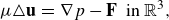
We are motivated by the conceptual model in Hernandez-Ortiz et al. (Reference Hernandez-Ortiz, Stoltz and Graham2005, Reference Hernández-Ortiz, de, Juan and Graham2009) and Underhill et al. (Reference Underhill, Hernandez-Ortiz and Graham2008) where the cell body and the flagellum are represented by different-sized spheres that instantaneously exert equal but opposite forces along the axis connecting their centres.
Figure 1. Schematic of the set-up for the derivation of the force-doublet model. Two regularised forces of equal magnitude in opposite directions have different size regularisation parameters. A limit as $\ell \to 0$
is taken in such a way that at
$\ell \to 0$
is taken in such a way that at ${\textbf{x}}_h$
,
${\textbf{x}}_h$
, ${\textbf{F}}({\textbf{x}}_h) ={\textbf{f}}(\ell ) \phi _{\epsilon _h}$
, with
${\textbf{F}}({\textbf{x}}_h) ={\textbf{f}}(\ell ) \phi _{\epsilon _h}$
, with ${\textbf{f}}(\ell ) = (q_0/\ell ) {\boldsymbol {\beta }}_0$
.
${\textbf{f}}(\ell ) = (q_0/\ell ) {\boldsymbol {\beta }}_0$
.
We consider two equal and opposite forces exerted at two different points separated by a distance $\ell$
in the direction of a unit vector
$\ell$
in the direction of a unit vector $ {\boldsymbol {\beta }}_0$
. In this case, the force,
$ {\boldsymbol {\beta }}_0$
. In this case, the force, ${\textbf{F}}({\textbf{x}}_h)$
, depends on the separation between the points. Referring to figure 1, the forces are applied at
${\textbf{F}}({\textbf{x}}_h)$
, depends on the separation between the points. Referring to figure 1, the forces are applied at ${\textbf{x}}_h$
and
${\textbf{x}}_h$
and ${\textbf{x}}_t$
, and we denote by
${\textbf{x}}_t$
, and we denote by ${\textbf{x}}_0$
the midpoint between them. The model will result from the limit as the points
${\textbf{x}}_0$
the midpoint between them. The model will result from the limit as the points ${\textbf{x}}_h$
and
${\textbf{x}}_h$
and ${\textbf{x}}_t$
approach
${\textbf{x}}_t$
approach ${\textbf{x}}_0$
. Here,
${\textbf{x}}_0$
. Here, $ {\boldsymbol {\beta }}_0$
is the unit vector from
$ {\boldsymbol {\beta }}_0$
is the unit vector from ${\textbf{x}}_t$
to
${\textbf{x}}_t$
to ${\textbf{x}}_h$
. We make two assumptions about the forces. The first one is that the regularisation parameters,
${\textbf{x}}_h$
. We make two assumptions about the forces. The first one is that the regularisation parameters, $\epsilon _h$
and
$\epsilon _h$
and $\epsilon _t$
, are different in order to break the symmetry of the system so that the velocity at
$\epsilon _t$
, are different in order to break the symmetry of the system so that the velocity at ${\textbf{x}}_0$
is non-zero and in the direction of
${\textbf{x}}_0$
is non-zero and in the direction of $ {\boldsymbol {\beta }}_0$
. Specifically, we set
$ {\boldsymbol {\beta }}_0$
. Specifically, we set $\epsilon _t=\epsilon - C\ell /2$
and
$\epsilon _t=\epsilon - C\ell /2$
and $\epsilon _h = \epsilon + C\ell /2$
for some constants
$\epsilon _h = \epsilon + C\ell /2$
for some constants $\epsilon$
and
$\epsilon$
and $C$
. The second assumption is that
$C$
. The second assumption is that ${\textbf{f}}(\ell )$
is inversely proportional to
${\textbf{f}}(\ell )$
is inversely proportional to $\ell$
, denoted by
$\ell$
, denoted by ${\textbf{f}}(\ell ) = (q_0/\ell ) {\boldsymbol {\beta }}_0$
for some constant
${\textbf{f}}(\ell ) = (q_0/\ell ) {\boldsymbol {\beta }}_0$
for some constant $q_0$
. This assumption is needed to prevent the two forces from simply cancelling each other.
$q_0$
. This assumption is needed to prevent the two forces from simply cancelling each other.
The fluid velocity they generate at an arbitrary point $\textbf{x}$
is
$\textbf{x}$
is
 \begin{align} S({\textbf{x}};{\textbf{x}}_h,\epsilon _h) q_0 {\boldsymbol {\beta }}_0/\ell - S({\textbf{x}};{\textbf{x}}_t,\epsilon _t) q_0 {\boldsymbol {\beta }}_0/\ell . \end{align}
We note that $S({\textbf{x}};{\textbf{x}}_h,\epsilon )$
depends on the difference
$S({\textbf{x}};{\textbf{x}}_h,\epsilon )$
depends on the difference ${\textbf{x}}-{\textbf{x}}_h$
, which is given by
${\textbf{x}}-{\textbf{x}}_h$
, which is given by ${\textbf{x}}-{\textbf{x}}_h = {\textbf{x}} - {\textbf{x}}_0 - (\ell /2) {\boldsymbol {\beta }}_0$
. Similarly,
${\textbf{x}}-{\textbf{x}}_h = {\textbf{x}} - {\textbf{x}}_0 - (\ell /2) {\boldsymbol {\beta }}_0$
. Similarly, ${\textbf{x}}-{\textbf{x}}_t = {\textbf{x}}-{\textbf{x}}_0+(\ell /2) {\boldsymbol {\beta }}_0$
. Therefore, the fluid velocity at
${\textbf{x}}-{\textbf{x}}_t = {\textbf{x}}-{\textbf{x}}_0+(\ell /2) {\boldsymbol {\beta }}_0$
. Therefore, the fluid velocity at $\textbf{x}$
can also be written as
$\textbf{x}$
can also be written as
 \begin{align} S({\textbf{x}}-{\textbf{x}}_0; (\ell /2) {\boldsymbol {\beta }}_0,\epsilon _h) q_0 {\boldsymbol {\beta }}_0/\ell - S({\textbf{x}}-{\textbf{x}}_0; - (\ell /2) {\boldsymbol {\beta }}_0,\epsilon _t) q_0 {\boldsymbol {\beta }}_0/\ell . \end{align}
With these assumptions, we take the limit as $\ell \to 0$
and find that the fluid velocity is
$\ell \to 0$
and find that the fluid velocity is
 \begin{eqnarray} {\textbf{u}}({\textbf{x}}) &=& - q_0 ( {\boldsymbol {\beta }}_0\cdot \nabla ) S({\textbf{x}};{\textbf{x}}_0,\epsilon _0) {\boldsymbol {\beta }}_0 +q_0 C \frac {\partial }{\partial \epsilon } S({\textbf{x}};{\textbf{x}}_0,\epsilon _0) {\boldsymbol {\beta }}_0. \end{eqnarray}
For the regularisation function $ {\phi _{\epsilon }}(r) = 15\epsilon ^4 (8\pi R^7)^{-1}$
, this is
$ {\phi _{\epsilon }}(r) = 15\epsilon ^4 (8\pi R^7)^{-1}$
, this is
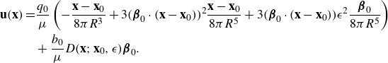
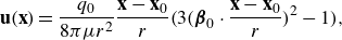
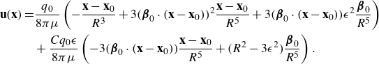 \begin{align} \begin{split} {\textbf{u}}({\textbf{x}})=& \frac {q_0}{8\pi \mu } \left ( - \frac {{\textbf{x}}-{\textbf{x}}_0}{R^3} + 3 ( {\boldsymbol {\beta }}_0\cdot ({\textbf{x}}-{\textbf{x}}_0))^2 \frac {{\textbf{x}}-{\textbf{x}}_0}{R^5} + 3( {\boldsymbol {\beta }}_0\cdot ({\textbf{x}}-{\textbf{x}}_0)) \epsilon ^2 \frac { {\boldsymbol {\beta }}_0}{R^5} \right )\\ &+ \frac {C q_0 \epsilon }{8\pi \mu } \left ( -3( {\boldsymbol {\beta }}_0\cdot ({\textbf{x}}-{\textbf{x}}_0)) \frac {{\textbf{x}}-{\textbf{x}}_0}{R^5} + \big ( R^2-3\epsilon ^2 \big ) \frac { {\boldsymbol {\beta }}_0}{R^5} \right ) . \end{split} \end{align}
The first term on the right side is the directional derivative of the Stokeslet in the direction of $ {\boldsymbol {\beta }}_0$
, and is therefore a stresslet. It turns out that the factor in parentheses in the last term is the regularised potential dipole
$ {\boldsymbol {\beta }}_0$
, and is therefore a stresslet. It turns out that the factor in parentheses in the last term is the regularised potential dipole
 \begin{equation} D({\textbf{x}};{\textbf{x}}_0,\epsilon ) {\boldsymbol {\beta }}_0 = - 3( {\boldsymbol {\beta }}_0\cdot ({\textbf{x}}-{\textbf{x}}_0)) \frac {{\textbf{x}}-{\textbf{x}}_0}{8\pi R^5} + \big ( R^2-3\epsilon ^2 \big ) \frac { {\boldsymbol {\beta }}_0}{8\pi R^5} , \end{equation}
which is derived from the regularising function $\phi _\epsilon (r)=3\epsilon ^2(4\pi R^5)^{-1}$
) (Cortez & Varela Reference Cortez and Varela2015). Defining
$\phi _\epsilon (r)=3\epsilon ^2(4\pi R^5)^{-1}$
) (Cortez & Varela Reference Cortez and Varela2015). Defining $b_0 = C q_0\epsilon$
, the fluid velocity at
$b_0 = C q_0\epsilon$
, the fluid velocity at $\textbf{x}$
is
$\textbf{x}$
is
 \begin{align} \begin{split} {\textbf{u}}({\textbf{x}})=& \frac {q_0}{\mu } \left ( - \frac {{\textbf{x}}-{\textbf{x}}_0}{8\pi R^3} + 3 ( {\boldsymbol {\beta }}_0\cdot ({\textbf{x}}-{\textbf{x}}_0))^2 \frac {{\textbf{x}}-{\textbf{x}}_0}{8\pi R^5} + 3( {\boldsymbol {\beta }}_0\cdot ({\textbf{x}}-{\textbf{x}}_0)) \epsilon ^2 \frac { {\boldsymbol {\beta }}_0}{8\pi R^5} \right ) \\&+ \frac {b_0 }{\mu } D({\textbf{x}};{\textbf{x}}_0,\epsilon ) {\boldsymbol {\beta }}_0 . \end{split} \end{align}
This is the proposed force-doublet model. We make the following comments.
-
(i) The self-propulsion of the particle is proportional to $b_0$
and is entirely provided by the potential dipole in the last term in the expression. Since the elements are regularised, the velocity is finite everywhere; in particular, it can be evaluated at
${\textbf{x}}={\textbf{x}}_0$
, yielding(2.11)For the particle to propel itself in the direction of
\begin{equation} {\textbf{u}}({\textbf{x}}_0) = \frac {b_0 }{\mu } D({\textbf{x}}_0;{\textbf{x}}_0,\epsilon ) {\boldsymbol {\beta }}_0 = - \frac { b_0 {\boldsymbol {\beta }}_0}{4\pi \mu \epsilon ^3}. \end{equation}
$ {\boldsymbol {\beta }}_0$
, we require
$b_0\lt 0$
.
$b_0$
and is entirely provided by the potential dipole in the last term in the expression. Since the elements are regularised, the velocity is finite everywhere; in particular, it can be evaluated at
${\textbf{x}}={\textbf{x}}_0$
, yielding(2.11)For the particle to propel itself in the direction of
\begin{equation} {\textbf{u}}({\textbf{x}}_0) = \frac {b_0 }{\mu } D({\textbf{x}}_0;{\textbf{x}}_0,\epsilon ) {\boldsymbol {\beta }}_0 = - \frac { b_0 {\boldsymbol {\beta }}_0}{4\pi \mu \epsilon ^3}. \end{equation}
$ {\boldsymbol {\beta }}_0$
, we require
$b_0\lt 0$
.
-
(ii) The first term in the velocity expression is a stresslet, and it is symmetric about the point
${\textbf{x}}_0$
so that replacing the factor
$({\textbf{x}}-{\textbf{x}}_0)$
with
$-({\textbf{x}}-{\textbf{x}}_0)$
results in a change in the sign of the stresslet term (see figures 2 and 3 following these comments). -
(iii) A particle located at
${\textbf{x}}_0$
with orientation vector
$ {\boldsymbol {\beta }}_0$
experiences a velocity
${\textbf{u}}({\textbf{x}}_0)$
due to itself and to other particles or obstacles nearby. The orientation vector is rotated by this flow according to Jeffery (Reference Jeffery1922), Saintillan (Reference Saintillan2018) and Tseng (Reference Tseng2022)(2.12)where
\begin{equation} \frac {\rm d}{{\rm d}t} {\boldsymbol {\beta }}_0 = \frac {1}{2} \Big ( \nabla \times {\textbf{u}}({\textbf{x}}_0) \Big ) \times {\boldsymbol {\beta }}_0 + \xi \Big ( I - {\boldsymbol {\beta }} {\boldsymbol {\beta }}^T \Big )\textbf{D} {\boldsymbol {\beta }}_0, \end{equation}
${\textbf{u}}({\textbf{x}}_0)$
is the fluid velocity at
${\textbf{x}}_0$
due to all elements, and
$\bf D$
is the rate-of-deformation tensor with components
$\textbf { D}_{ij} = \frac {1}{2}(\partial u_i/\partial x_j + \partial u_j/\partial x_i)$
. The parameter
$\xi$
is a factor that depends on the shape of the particle. For a spherical particle,
$\xi =0$
, while for a slender particle,
$\xi =1$
. As this article is concerned with reduced models of flagellated organisms, we consider the case of
$\xi =1$
, which simplifies the orientation vector equation to(2.13)
\begin{equation} \frac {\rm d}{{\rm d}t} {\boldsymbol {\beta }}_0 = [ {\boldsymbol {\beta }}_0 \times ( {\boldsymbol {\beta }}_0 \cdot \nabla ){\textbf{u}}({\textbf{x}}_0)]\times {\boldsymbol {\beta }}_0 . \end{equation}
-
(iv) The velocity field along the axis of the organism,
${\textbf{x}} = {\textbf{x}}_0 + s {\boldsymbol {\beta }}_0$
for
$-\infty \lt s \lt \infty$
, includes a stagnation point located at
${\textbf{x}}_{sp} = {\textbf{x}}_0 + (b_0/q_0) {\boldsymbol {\beta }}_0$
. The motion of an organism classified as a ‘pusher’ will typically generate a stagnation point downstream from the cell body, which corresponds to choosing
$q_0\gt 0$
in the model. On the other hand, a puller will typically generate a flow with a stagnation point in front of the cell body. This case corresponds to
$q_0\lt 0$
.


2.3. The complete formulation
In this study, we used the regularisation function that is most commonly used with the method of regularised Stokeslets (Cortez et al. Reference Cortez, Fauci and Medovikov2005). The derivation of the reduced model presented here can be done with a different regularisation function, if desired. In general, the flow at an arbitrary location $\textbf{x}$
may involve contributions from
$\textbf{x}$
may involve contributions from $N_d$
force doublets with parameters
$N_d$
force doublets with parameters $(q_{j}, b_j, {\boldsymbol {\beta }}_j)$
located at
$(q_{j}, b_j, {\boldsymbol {\beta }}_j)$
located at ${\textbf{x}}_j$
, and possibly from
${\textbf{x}}_j$
, and possibly from $N_f$
forces
$N_f$
forces ${\textbf{f}}_k$
located at
${\textbf{f}}_k$
located at $\textbf{y}_k$
generated by solid boundaries, steric forces or other mechanisms. The total fluid velocity at
$\textbf{y}_k$
generated by solid boundaries, steric forces or other mechanisms. The total fluid velocity at $\textbf{x}$
due to these elements is the superposition of all of the elements.
$\textbf{x}$
due to these elements is the superposition of all of the elements.
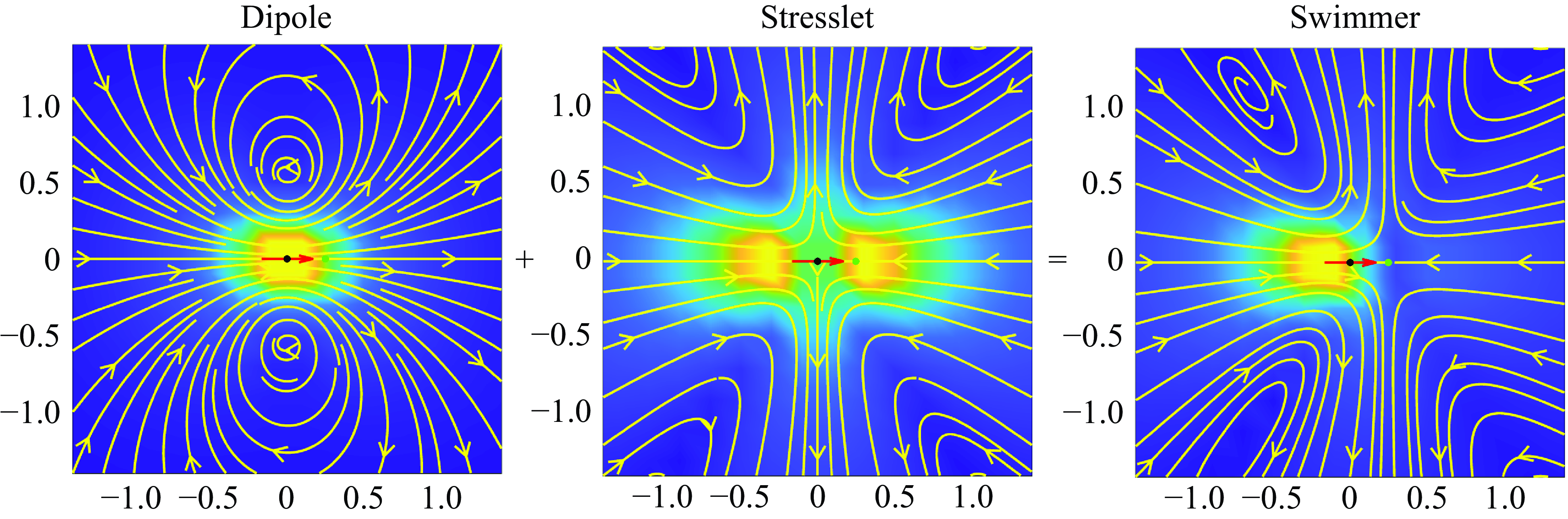
Figure 2. The fluid velocity produced by the model ‘puller’ particle is the sum of a potential dipole (left) and a stresslet (middle). The arrow shows the swimming direction and the black dot in the centre of the arrow is the particle location. The green dot in front of the particle is the stagnation point. The parameters used were $\epsilon = 0.4$
,
$\epsilon = 0.4$
, $b_0 = -1$
,
$b_0 = -1$
, $q_0 = -4$
, so that the stagnation point is located at
$q_0 = -4$
, so that the stagnation point is located at $b_0/q_0 = 1/4$
.
$b_0/q_0 = 1/4$
.
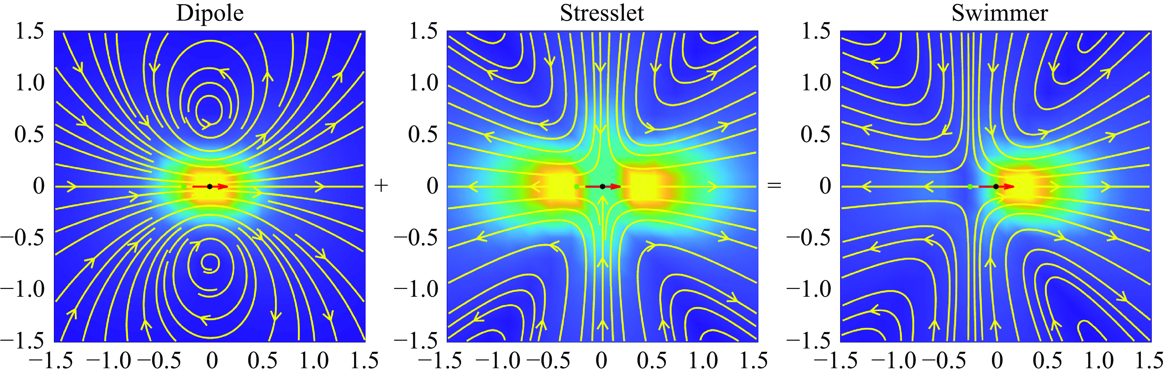
Figure 3. The fluid velocity produced by the model ‘pusher’ particle is the sum of a potential dipole (left) and a stresslet (middle). The arrow shows the swimming direction and the black dot in the centre of the arrow is the particle location. The green dot behind the particle is the stagnation point. The parameters used were $\epsilon = 0.4$
,
$\epsilon = 0.4$
, $b_0 = -1$
,
$b_0 = -1$
, $q_0 = 4$
, so that the stagnation point is located at
$q_0 = 4$
, so that the stagnation point is located at $b_0/q_0 = -1/4$
.
$b_0/q_0 = -1/4$
.
It is convenient to write the model equations in dimensionless form in order to identify dimensionless groups and reduce the number of parameters. A characteristic length and a characteristic speed for the problem are needed. Here, we use $\epsilon$
as the normalising length scale and the swimming speed
$\epsilon$
as the normalising length scale and the swimming speed $v_0$
as the characteristic speed. Time will be scaled by
$v_0$
as the characteristic speed. Time will be scaled by $\epsilon /v_0$
. We use the notation
$\epsilon /v_0$
. We use the notation $\tilde {\textbf { x}} = {\textbf { x}}/\epsilon$
,
$\tilde {\textbf { x}} = {\textbf { x}}/\epsilon$
, $\tilde {\textbf { y}} = {\textbf { y}}/\epsilon$
,
$\tilde {\textbf { y}} = {\textbf { y}}/\epsilon$
, $\tilde R = R/\epsilon$
,
$\tilde R = R/\epsilon$
, $\tilde t = t v_0/\epsilon$
and
$\tilde t = t v_0/\epsilon$
and $\tilde {\textbf { u}} = {\textbf { u}}/v_0$
to write the equation for the velocity due to forces, force doublets and rotlet doubles as
$\tilde {\textbf { u}} = {\textbf { u}}/v_0$
to write the equation for the velocity due to forces, force doublets and rotlet doubles as
 \begin{align} &\tilde {\textbf{u}}({\textbf{x}})\nonumber\\ &= \sum _{k=1}^M \left ( \frac {{\textbf{f}}_k}{\mu v_0\epsilon } \right ) \left ( \frac {1}{8\pi \tilde R_k}+\frac {1}{ 8\pi \tilde R_k^3} \right ) + \left ( \frac {{\textbf{f}}_k}{\mu |v_0|\epsilon } \right ) \cdot (\tilde {\textbf{x}}-\tilde {\textbf { y}}_k) \frac {(\tilde {\textbf{x}}-\tilde {\textbf { y}}_k)}{ 8\pi \tilde R_k^3} \nonumber \\ & + \sum _{j=1}^N \left ( \frac {q_j }{\mu v_0 \epsilon ^2} \right ) \left ( - \frac {\tilde {\textbf{x}}-\tilde {\textbf{x}}_j}{ 8\pi \tilde R_j^3} + 3 ( {\boldsymbol {\beta }}_j\cdot (\tilde {\textbf{x}}-\tilde {\textbf{x}}_j))^2 \frac {\tilde {\textbf{x}}-\tilde {\textbf{x}}_j}{ 8\pi \tilde R_j^5} + 3( {\boldsymbol {\beta }}_j\cdot (\tilde {\textbf{x}}-\tilde {\textbf{x}}_j)) \frac { {\boldsymbol {\beta }}_j}{ 8\pi \tilde R_j^5} \right ) \nonumber \\ &+ \left ( \frac {b_j }{ \mu v_0 \epsilon ^3} \right ) \left ( - 3( {\boldsymbol {\beta }}_j\cdot (\tilde {\textbf{x}}-\tilde {\textbf{x}}_j)) \frac {\tilde {\textbf{x}}-\tilde {\textbf{x}}_j}{ 8\pi \tilde R_j^5} + \big ( \tilde R_j^2-3 \big ) \frac { {\boldsymbol {\beta }}_j}{ 8\pi \tilde R_j^5} \right ), \end{align}
where the following dimensionless coefficients are identified
 \begin{equation} \tilde {\textbf{f}}_k = \frac {{\textbf{f}}_k}{\mu v_0\epsilon } ,\ \ \ \ \ \ \tilde q_j = \frac {q_j }{\mu v_0 \epsilon ^2},\ \ \ \ \ \ \tilde b_j = \frac {b_j }{ \mu v_0 \epsilon ^3}. \ \ \ \ \ \ \end{equation}
The change in the orientation $\boldsymbol {\beta }_n$
of the force doublet at
$\boldsymbol {\beta }_n$
of the force doublet at $\mathbf {x}_n$
is computed with Jeffery’s equation (Jeffery Reference Jeffery1922)
$\mathbf {x}_n$
is computed with Jeffery’s equation (Jeffery Reference Jeffery1922)
 \begin{equation} \frac {\rm d}{{\rm d}t} \boldsymbol {\beta }_n = [ \boldsymbol {\beta }_n \times (\boldsymbol {\beta }_n\cdot \nabla ){\textbf{u}}({\textbf{x}}_n)]\times \boldsymbol {\beta }_n .\end{equation}
The expressions for the velocity gradients are found by differentiating the velocity expression and are given in Appendix A.
3. Results
This section presents studies performed using the force-doublet model. First, we explore the choice of model parameters discussed in § 2.2. Then, we examine the stability of two particles swimming parallel to each other. Next, we demonstrate the potential of the framework to incorporate other flow characteristics by incorporating rotlet doubles into the force-doublet framework. Lastly, we employ the method of images for a force doublet interacting with an infinite plane wall.
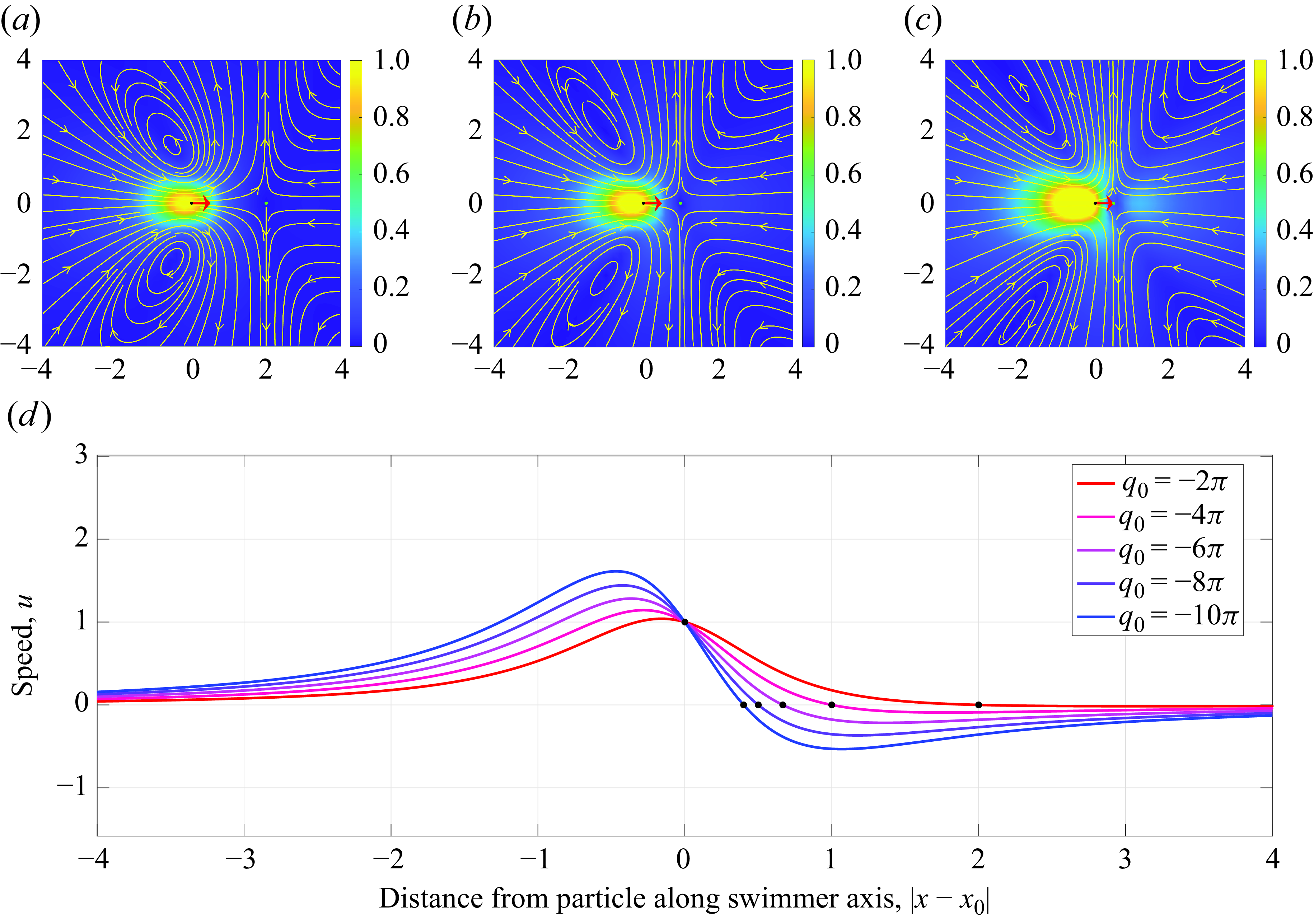
Figure 4. Plots of the velocity streamlines along the centre plane of the force doublet ( $v_0=1.0$
,
$v_0=1.0$
, $\delta =1.0$
,
$\delta =1.0$
, $b_0=-4\pi$
) over the scalar field of the velocity magnitude for (a)
$b_0=-4\pi$
) over the scalar field of the velocity magnitude for (a) $q_0=-2\pi$
, (b)
$q_0=-2\pi$
, (b) $q_0=-4\pi$
and (c)
$q_0=-4\pi$
and (c) $q_0=-8\pi$
, along with (d) the speed
$q_0=-8\pi$
, along with (d) the speed $u$
plot plotted along the centre axis for varying
$u$
plot plotted along the centre axis for varying $q_0$
. Note that, while the velocity is held fixed, the resulting stagnation point approaches the origin as
$q_0$
. Note that, while the velocity is held fixed, the resulting stagnation point approaches the origin as $q_0$
increases.
$q_0$
increases.
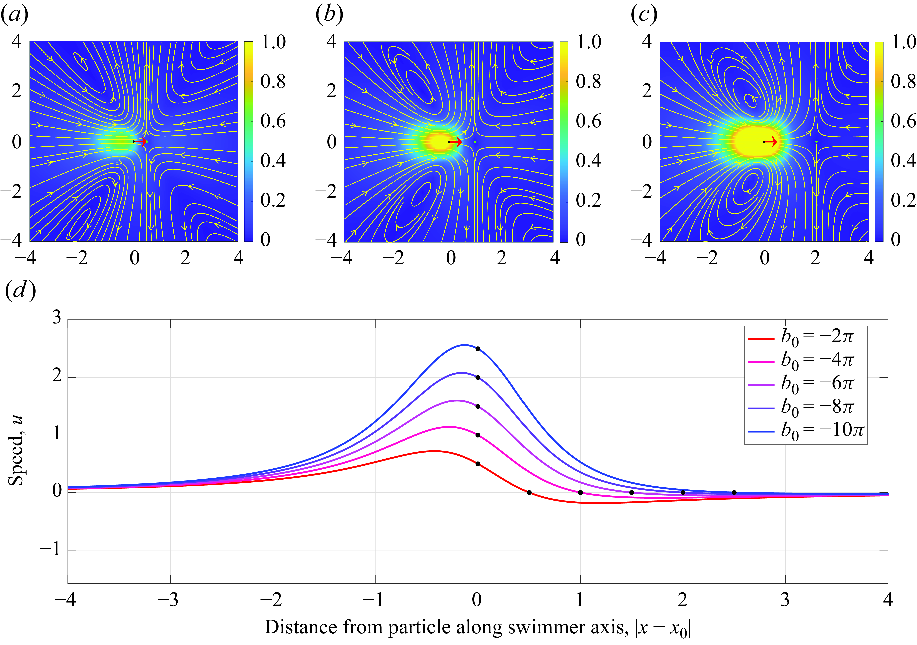
Figure 5. Plots of the velocity streamlines along the centre plane of the force doublet ( $v_0=1.0$
,
$v_0=1.0$
, $\epsilon =1.0$
,
$\epsilon =1.0$
, $q_0=-4\pi$
) over the scalar field of the velocity magnitude for (a)
$q_0=-4\pi$
) over the scalar field of the velocity magnitude for (a) $b_0=-2\pi$
, (b)
$b_0=-2\pi$
, (b) $b_0=-4\pi$
and (c)
$b_0=-4\pi$
and (c) $b_0=-8\pi$
, along with (d) the speed
$b_0=-8\pi$
, along with (d) the speed $u$
plot plotted along the centre axis for varying
$u$
plot plotted along the centre axis for varying $b_0$
. Note that, while the velocity is held fixed, the resulting stagnation point approaches the origin as
$b_0$
. Note that, while the velocity is held fixed, the resulting stagnation point approaches the origin as $q_0$
increases.
$q_0$
increases.
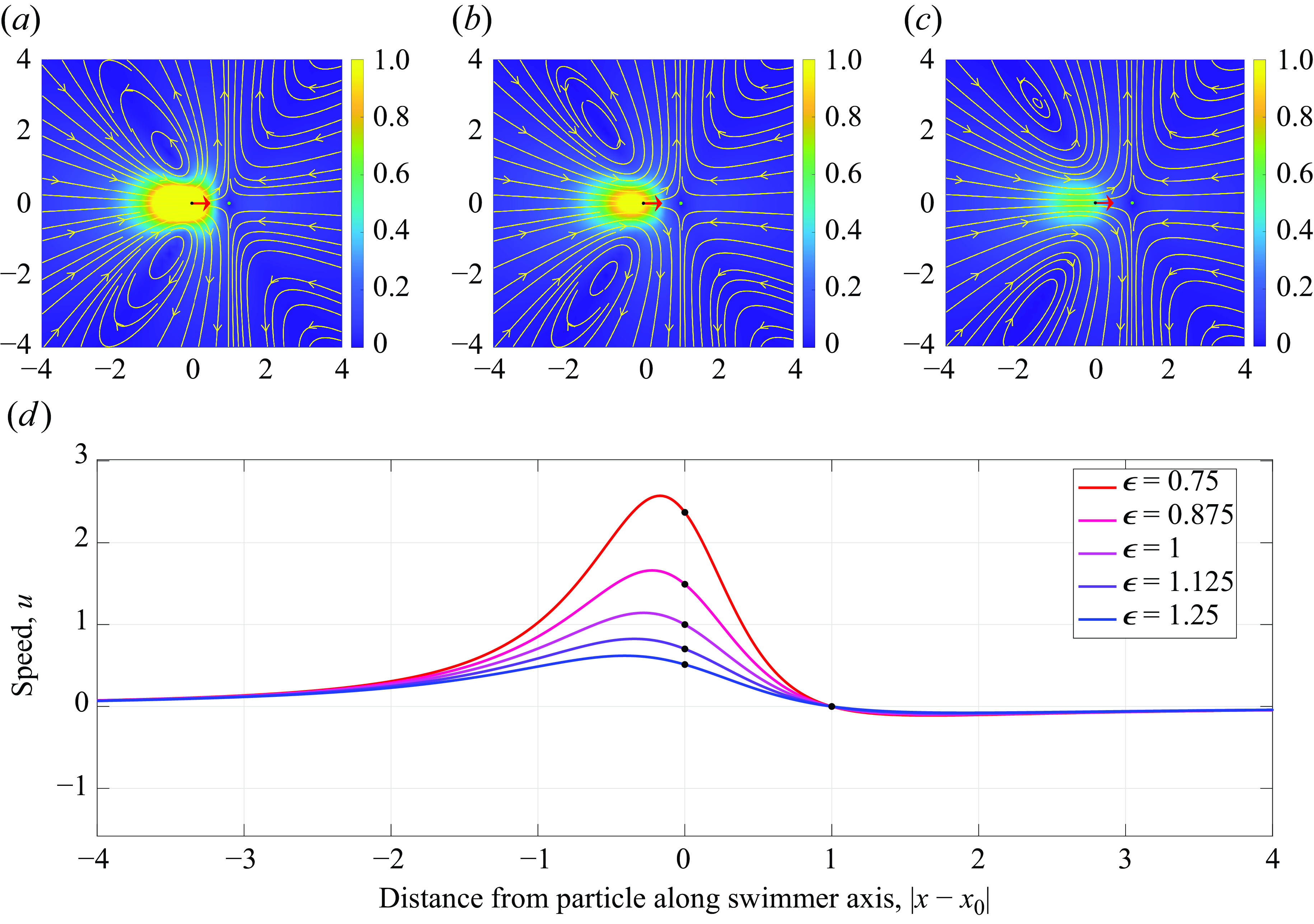
Figure 6. Plots of the velocity streamlines along the centre plane of the force doublet ( $b_0=-4\pi$
,
$b_0=-4\pi$
, $q_0=-s4\pi$
) over the scalar field of the velocity magnitude for (a)
$q_0=-s4\pi$
) over the scalar field of the velocity magnitude for (a) $\epsilon =0.75$
, (b)
$\epsilon =0.75$
, (b) $\epsilon =1.0$
and (c)
$\epsilon =1.0$
and (c) $\epsilon =1.25$
, along with (d) the speed
$\epsilon =1.25$
, along with (d) the speed $u$
plot plotted along the centre axis for varying
$u$
plot plotted along the centre axis for varying $\epsilon$
. Note that the stagnation point is held fixed, although the resulting self-swimming velocity increases as
$\epsilon$
. Note that the stagnation point is held fixed, although the resulting self-swimming velocity increases as $\epsilon$
decreases.
$\epsilon$
decreases.
3.1. Parameter selection
The choice of parameters in the force-doublet model of (2.10) is dependent on the organismal system. Importantly, the model parameters can be estimated experimentally based on the organism’s swimming velocity, its geometry and features of the flow it generates.
Using the self-velocity shown in (2.11), in order to model a swimmer with a cycle-averaged swimming speed of $v_0$
, we choose
$v_0$
, we choose
 \begin{equation} b_0 = -4\pi \mu \epsilon ^3 v_0, \end{equation}
from which the stagnation point, $s_0=b_0/q_0$
, could be used as a constraint for describing flow features.
$s_0=b_0/q_0$
, could be used as a constraint for describing flow features.
In figure 4(a–c), we plot the resulting velocity streamlines along the central plane over the scalar field of the velocity magnitude of puller for varying $q_0$
. Here,
$q_0$
. Here, $b_0$
is fixed for a velocity
$b_0$
is fixed for a velocity $v_0=1.0$
and
$v_0=1.0$
and $\epsilon =1.0$
. Initially setting
$\epsilon =1.0$
. Initially setting $q_0=-4\pi$
yields a stagnation point at
$q_0=-4\pi$
yields a stagnation point at $x=1.0$
(figure 4
a), increasing (figure 4
b,c)
$x=1.0$
(figure 4
a), increasing (figure 4
b,c) $q_0$
leads to a shift in the stagnation point towards
$q_0$
leads to a shift in the stagnation point towards $x_0$
, following the reciprocal relation of
$x_0$
, following the reciprocal relation of $1/q_0$
for a fixed
$1/q_0$
for a fixed $b_0$
. Plotting the velocity along the centre line in figure 4(d), we note the change in the resulting flow profile as
$b_0$
. Plotting the velocity along the centre line in figure 4(d), we note the change in the resulting flow profile as $|q_0|$
increases, where the flow anti-symmetry associated with the stresslet becomes more pronounced.
$|q_0|$
increases, where the flow anti-symmetry associated with the stresslet becomes more pronounced.
Similarly, varying $b_0$
, in figure 5, we note the role the dipole plays in determining the resulting flow profile. Given the initial flow profile of a puller in figure 5(a) for
$b_0$
, in figure 5, we note the role the dipole plays in determining the resulting flow profile. Given the initial flow profile of a puller in figure 5(a) for $b_0=-2\pi$
, we note that as
$b_0=-2\pi$
, we note that as $b_0$
increases (figure 5
b,c) the strength of the dipole contribution increases as well. This corresponds to an increase in the self-swimming velocity at
$b_0$
increases (figure 5
b,c) the strength of the dipole contribution increases as well. This corresponds to an increase in the self-swimming velocity at $x_0$
, as seen when plotting the velocity on the centre line (figure 5
d). Increasing
$x_0$
, as seen when plotting the velocity on the centre line (figure 5
d). Increasing $b_0$
also increases the resulting stagnation point, due to its linear relationship with
$b_0$
also increases the resulting stagnation point, due to its linear relationship with $b_0$
for a fixed
$b_0$
for a fixed $q_0$
.
$q_0$
.
Varying the regularisation parameter $\epsilon$
also affects the resulting flow field. Plotting the resulting flow fields for varying
$\epsilon$
also affects the resulting flow field. Plotting the resulting flow fields for varying $\epsilon$
, given a fixed
$\epsilon$
, given a fixed $b_0=-4\pi$
and
$b_0=-4\pi$
and $q_0=-4\pi$
, in figure 6(a), we note how increasing
$q_0=-4\pi$
, in figure 6(a), we note how increasing $\epsilon$
spreads the resulting flow field, as is natural to associate with a regularisation parameter. Plotting the centre line velocity in figure 6(d), we note that the choice of the regularisation parameter does affect the resulting self-swimming speed, given that it is proportional to
$\epsilon$
spreads the resulting flow field, as is natural to associate with a regularisation parameter. Plotting the centre line velocity in figure 6(d), we note that the choice of the regularisation parameter does affect the resulting self-swimming speed, given that it is proportional to $1/\epsilon ^3$
(3.1). However, given the fixed choice of
$1/\epsilon ^3$
(3.1). However, given the fixed choice of $b_0$
and
$b_0$
and $q_0$
, the resulting stagnation point remains fixed.
$q_0$
, the resulting stagnation point remains fixed.
Biologically relevant values of $q_0$
can be determined by considering the velocity given by the model along the organism’s axis. One characteristic of a pusher is that the fluid motion along the organism’s axis shows a stagnation point located at a distance of
$q_0$
can be determined by considering the velocity given by the model along the organism’s axis. One characteristic of a pusher is that the fluid motion along the organism’s axis shows a stagnation point located at a distance of $b_0/q_0$
behind the cell body position, where the stresslet flow balances the dipole flow. For a puller, the stagnation point is also at a distance of
$b_0/q_0$
behind the cell body position, where the stresslet flow balances the dipole flow. For a puller, the stagnation point is also at a distance of $b_0/q_0$
from the cell body position, but upstream from it. If we consider
$b_0/q_0$
from the cell body position, but upstream from it. If we consider ${\textbf{x}}_0$
the centre of the cell body, then the distance
${\textbf{x}}_0$
the centre of the cell body, then the distance $s_0$
from
$s_0$
from ${\textbf{x}}_0$
to the stagnation point provides a length scale for the organism and can be estimated experimentally (see e.g. Drescher et al. Reference Drescher, Dunkel, Cisneros, Ganguly and Goldstein2011; Mondal et al. Reference Mondal, Prabhune, Ramaswamy and Sharma2021). These parameters in turn allow one to fit the model to a cycle-averaged flow field, as was done, for example, in Ishimoto et al. (Reference Ishimoto, Gaffney and Walker2020) and Delmotte et al. (Reference Delmotte, Keaveny, Plouraboué and Climent2015). For our model, experimental data can then provide an estimate for
${\textbf{x}}_0$
to the stagnation point provides a length scale for the organism and can be estimated experimentally (see e.g. Drescher et al. Reference Drescher, Dunkel, Cisneros, Ganguly and Goldstein2011; Mondal et al. Reference Mondal, Prabhune, Ramaswamy and Sharma2021). These parameters in turn allow one to fit the model to a cycle-averaged flow field, as was done, for example, in Ishimoto et al. (Reference Ishimoto, Gaffney and Walker2020) and Delmotte et al. (Reference Delmotte, Keaveny, Plouraboué and Climent2015). For our model, experimental data can then provide an estimate for $s_0$
, which determines
$s_0$
, which determines $q_0=b_0/s_0$
. In figure 7(a), we present a choice of parameters (
$q_0=b_0/s_0$
. In figure 7(a), we present a choice of parameters ( $b_0=-40\pi , q_0=20\pi , \epsilon =1.0$
) that match many of the experimental flow features of a pusher bacteria described in Drescher et al. (Reference Drescher, Dunkel, Cisneros, Ganguly and Goldstein2011) (figure 7
b). Similarly, we can produce qualitatively similar flow fields (
$b_0=-40\pi , q_0=20\pi , \epsilon =1.0$
) that match many of the experimental flow features of a pusher bacteria described in Drescher et al. (Reference Drescher, Dunkel, Cisneros, Ganguly and Goldstein2011) (figure 7
b). Similarly, we can produce qualitatively similar flow fields ( $b_0=-80000\pi , q_0=-4000\pi , \epsilon =10.0$
) to those reported in Mondal et al. (Reference Mondal, Prabhune, Ramaswamy and Sharma2021), as shown in figures 7(c) and 7(d).
$b_0=-80000\pi , q_0=-4000\pi , \epsilon =10.0$
) to those reported in Mondal et al. (Reference Mondal, Prabhune, Ramaswamy and Sharma2021), as shown in figures 7(c) and 7(d).
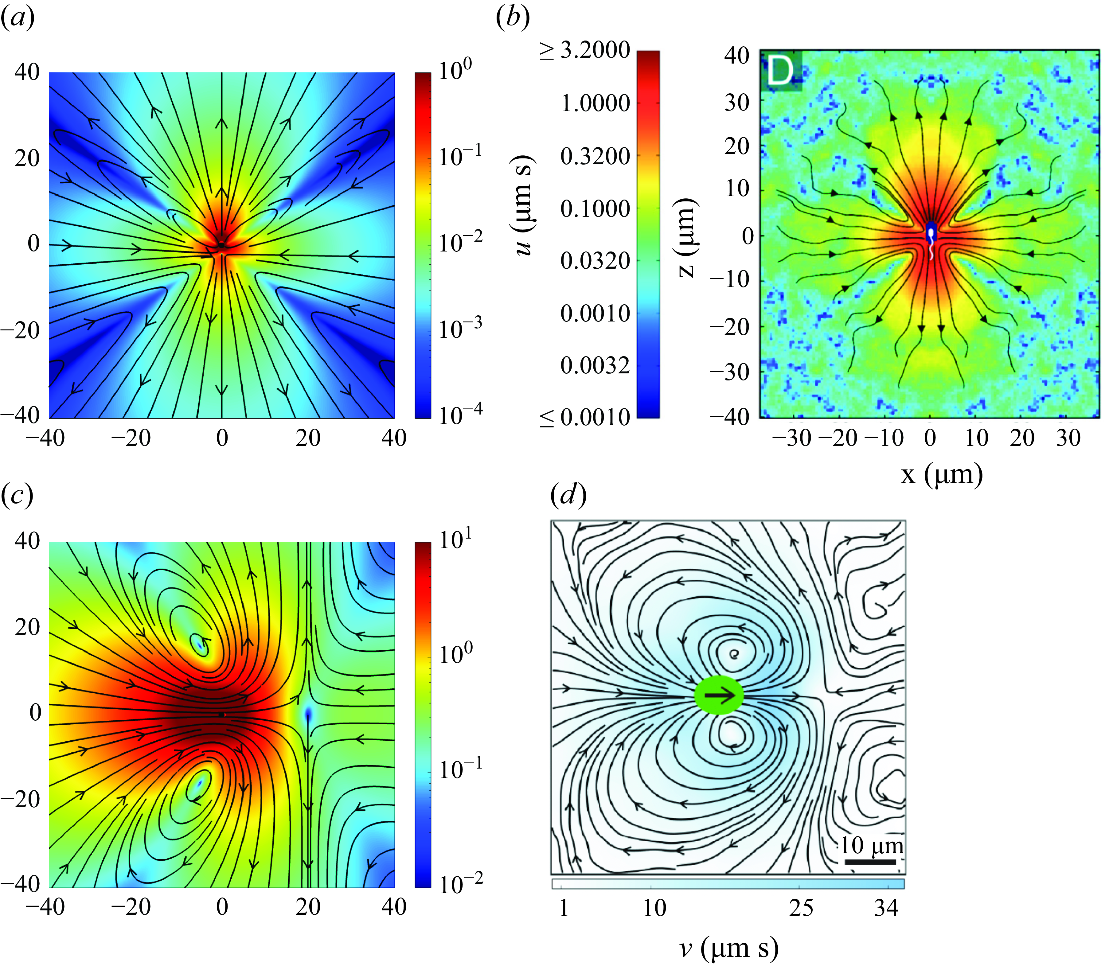
Figure 7. Flow comparisons of the flow magnitude and contours of (a) the force-doublet model of a pusher, using $b_0=-40\pi , q_0=20\pi $
and
$b_0=-40\pi , q_0=20\pi $
and $ \epsilon =1.0$
, with (b) experimental recordings from Drescher et al. (Reference Drescher, Dunkel, Cisneros, Ganguly and Goldstein2011). Similar flow comparisons can also be made with (c) the model, using
$ \epsilon =1.0$
, with (b) experimental recordings from Drescher et al. (Reference Drescher, Dunkel, Cisneros, Ganguly and Goldstein2011). Similar flow comparisons can also be made with (c) the model, using $b_0=-80000\pi , q_0=-4000\pi $
and
$b_0=-80000\pi , q_0=-4000\pi $
and $\epsilon =10.0$
with (d) experimental flows from Mondal et al. (Reference Mondal, Prabhune, Ramaswamy and Sharma2021).
$\epsilon =10.0$
with (d) experimental flows from Mondal et al. (Reference Mondal, Prabhune, Ramaswamy and Sharma2021).
3.2. Dynamics of two pusher swimmers moving parallel to each other
We consider a scenario in which two identical particles translate parallel to each other along the paths ${\textbf{x}}_1(t)$
and
${\textbf{x}}_1(t)$
and ${\textbf{x}}_2(t)$
, with initial conditions given by
${\textbf{x}}_2(t)$
, with initial conditions given by ${\textbf{x}}_1(0) = (0,y_0,0)$
and
${\textbf{x}}_1(0) = (0,y_0,0)$
and ${\textbf{x}}_2(0) = (0,-y_0,0)$
with
${\textbf{x}}_2(0) = (0,-y_0,0)$
with $y_0\gt 0$
. Therefore, the separation distance between them is
$y_0\gt 0$
. Therefore, the separation distance between them is $r_0=2y_0$
. We are interested in the motion that translates the particles at a constant speed in the
$r_0=2y_0$
. We are interested in the motion that translates the particles at a constant speed in the $x$
-direction. That is, the particle velocities are
$x$
-direction. That is, the particle velocities are $(U,0,0)$
where
$(U,0,0)$
where $U$
is a constant. In addition, the orientation vectors are assumed to be fixed in time so that
$U$
is a constant. In addition, the orientation vectors are assumed to be fixed in time so that $\rm d {\boldsymbol {\beta }}/{\rm d}\textit{t}=0$
. A similar situation is discussed in Lushi & Peskin (Reference Lushi and Peskin2013).
$\rm d {\boldsymbol {\beta }}/{\rm d}\textit{t}=0$
. A similar situation is discussed in Lushi & Peskin (Reference Lushi and Peskin2013).
Given parameters $\epsilon$
,
$\epsilon$
, $q_0$
,
$q_0$
, $b_0$
, the symmetry of the problem implies that the orientation vector of particle one is
$b_0$
, the symmetry of the problem implies that the orientation vector of particle one is $(\beta _1, -\beta _2, 0)$
and the orientation vector of the second particle is
$(\beta _1, -\beta _2, 0)$
and the orientation vector of the second particle is $(\beta _1,\beta _2,0)$
. The unknowns are the separation distance
$(\beta _1,\beta _2,0)$
. The unknowns are the separation distance $r_0$
, the orientation vector component
$r_0$
, the orientation vector component $\beta _2$
, and the speed
$\beta _2$
, and the speed $U$
.
$U$
.
The dimensionless velocity of the top particle (the fluid velocity at ${\textbf{x}}_1(t)$
) is given by (A2) with
${\textbf{x}}_1(t)$
) is given by (A2) with $N=2$
,
$N=2$
, ${\textbf{f}}=0$
and
${\textbf{f}}=0$
and ${\textbf{x}}-{\textbf{x}}_j=(0,r_0,0)$
. The rate of change of the orientation vector is given by (2.13). Since the motion in this example takes place in the
${\textbf{x}}-{\textbf{x}}_j=(0,r_0,0)$
. The rate of change of the orientation vector is given by (2.13). Since the motion in this example takes place in the $xy$
-plane, the two non-zero components of the orientation vector have the same rate of change, so they lead to a single constraint equation. In component form, the unknown variables satisfy
$xy$
-plane, the two non-zero components of the orientation vector have the same rate of change, so they lead to a single constraint equation. In component form, the unknown variables satisfy
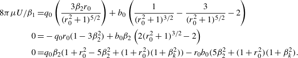 \begin{align} \begin{split} 8\pi \mu U/\beta _1 = & q_0 \left ( \frac { 3\beta _2 r_0 }{(r_0^2+1)^{5/2}} \right ) + b_0 \left ( \frac {1}{ (r_0^2+1)^{3/2}} - \frac { 3 }{ (r_0^2+1)^{5/2}} - 2 \right ) \\ 0 = & - q_0 r_0 (1-3 \beta _2^2) + b_0 \beta _2 \left ( 2 (r_0^2+1)^{3/2} - 2 \right ) \\ 0 = & q_0 \beta _2(1 + r_0^2 - 5\beta _2^2 + (1+r_0^2)(1+\beta _k^2) ) - r_0 b_0 (5\beta _2^2 + (1+r_0^2)(1+\beta _k^2). \end{split} \end{align}
The last two equations can be solved numerically for $\beta _2$
and
$\beta _2$
and $r_0$
using Newton’s method (figure 8
a). Once those two variables are known, the swimming speed
$r_0$
using Newton’s method (figure 8
a). Once those two variables are known, the swimming speed $U$
is found from the first equation. In the case of a pusher, the solution is
$U$
is found from the first equation. In the case of a pusher, the solution is $r_0 = 0.11540745284558$
,
$r_0 = 0.11540745284558$
, $\beta _2 = 0.4730561821293$
and
$\beta _2 = 0.4730561821293$
and $U = 1.6928$
.
$U = 1.6928$
.
We make the observation that changing the signs of $q_0$
and
$q_0$
and $\beta _2$
leaves the three equations above unchanged. Recall that
$\beta _2$
leaves the three equations above unchanged. Recall that $q_0\gt 0$
corresponds to a pusher and
$q_0\gt 0$
corresponds to a pusher and $q_0\lt 0$
corresponds to a puller. Thus, we conclude that two pullers also can move parallel to one another at the same separation distance as the pushers, but with the orientation vectors tilted toward one another instead of away from each other (figure 8
b).
$q_0\lt 0$
corresponds to a puller. Thus, we conclude that two pullers also can move parallel to one another at the same separation distance as the pushers, but with the orientation vectors tilted toward one another instead of away from each other (figure 8
b).
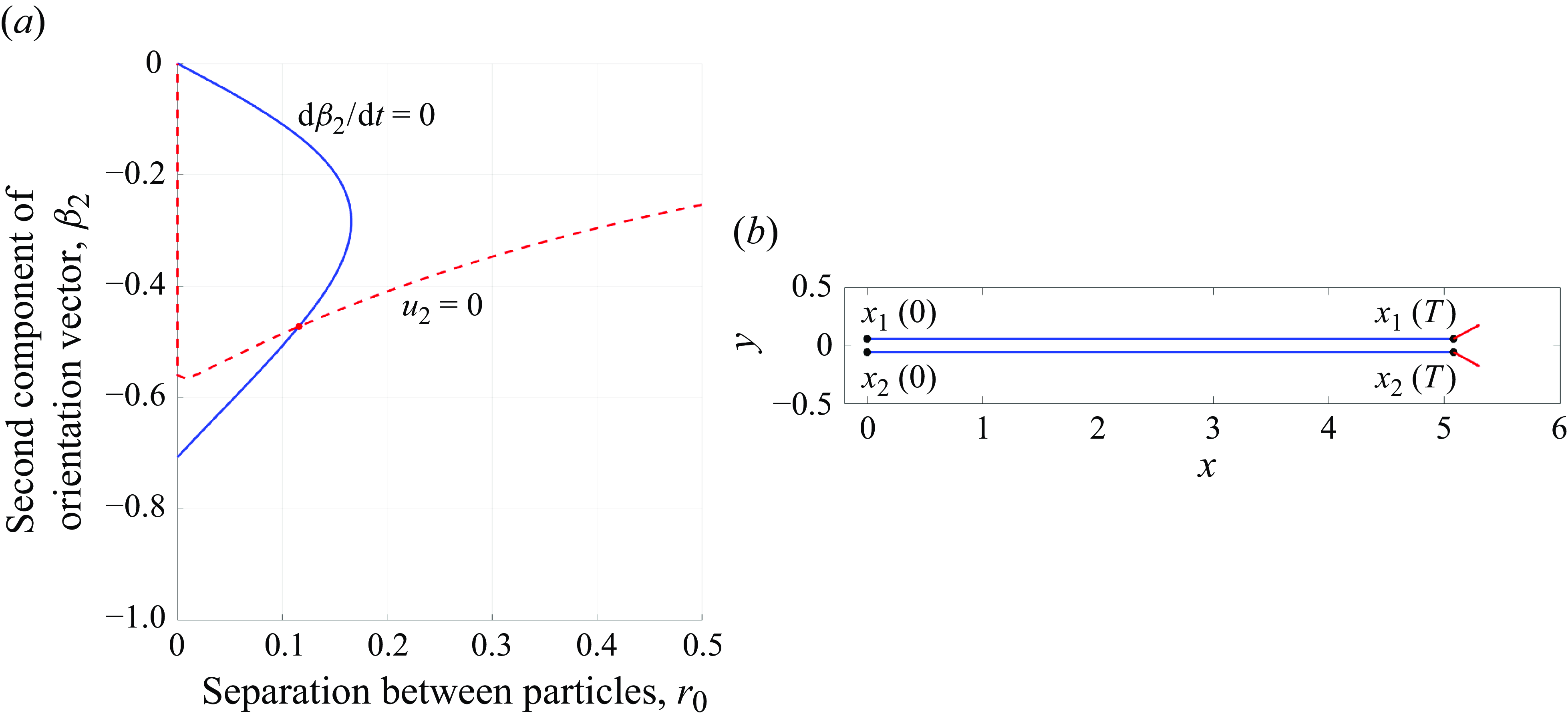
Figure 8. (a) Equilibrium point for two force doublets translating along the $x$
-direction at constant speed parallel to each other. The curve where the
$x$
-direction at constant speed parallel to each other. The curve where the $y$
-component of velocity of the particles is zero (red dashed) and the curve where the rate of change of their orientation vectors is zero (blue solid) are shown. (b) The trajectories of the particles for
$y$
-component of velocity of the particles is zero (red dashed) and the curve where the rate of change of their orientation vectors is zero (blue solid) are shown. (b) The trajectories of the particles for $t\in [0,3]$
. The coordinates of the intersection point give the particle separation and orientation vector that produce this motion. The dimensionless parameters used were
$t\in [0,3]$
. The coordinates of the intersection point give the particle separation and orientation vector that produce this motion. The dimensionless parameters used were $q_0 = 2\pi$
,
$q_0 = 2\pi$
, $b_0 = -4\pi$
,
$b_0 = -4\pi$
, $\epsilon =1$
and
$\epsilon =1$
and $\mu = 1$
. The separation distance between the particles was approximately
$\mu = 1$
. The separation distance between the particles was approximately $r_0 = 0.11541$
and the orientation vectors were approximately
$r_0 = 0.11541$
and the orientation vectors were approximately $\hat \beta = (0.88103, \pm 0.47305,0)$
.
$\hat \beta = (0.88103, \pm 0.47305,0)$
.
3.3. Including the effect of torques with rotlet doubles
So far, the presentation of the reduced model has been based on a force dipole along the axis of the swimmer. However, a more comprehensive model would also include the effect of torques that are generated, for example, in the case of bacteria with rotating helical flagella (Spagnolie & Lauga Reference Spagnolie and Lauga2012; Ishimoto et al. Reference Ishimoto, Gaffney and Walker2020). Here, we describe how to include this rotational flow.
The main idea used to derive the model was to take the limit as two equal and opposite regularised elements approached each other with an asymmetry in the regularisation parameter. Using Stokeslets as the regularised elements resulted in applying the operator
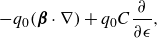 \begin{align} - q_0 ( {\boldsymbol {\beta }}\cdot \nabla ) +q_0 C \frac {\partial }{\partial \epsilon } , \end{align}
to the Stokeslet, as described in (2.7). The same procedure, which has been validated experimentally (Yamamoto & Sano Reference Yamamoto and Sano2018), can be applied with a rotlet replacing the Stokeslet to include the effect of torques. Specifically, the fluid velocity due to a regularised rotlet of strength $q_0^r {\boldsymbol {\beta }}$
is given by
$q_0^r {\boldsymbol {\beta }}$
is given by
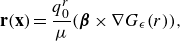 \begin{equation} \mathbf {r}(\mathbf {x})= \frac {q_0^r}{\mu } ( {\boldsymbol {\beta }}\times \nabla G_\epsilon (r)), \end{equation}
where we recall that $\triangle G_\epsilon = \phi _\epsilon$
. Thus, the velocity at
$\triangle G_\epsilon = \phi _\epsilon$
. Thus, the velocity at $\mathbf {x}$
due to an asymmetric rotlet double located at the origin is
$\mathbf {x}$
due to an asymmetric rotlet double located at the origin is
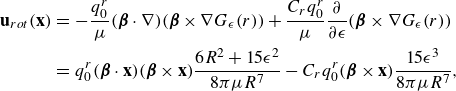 \begin{eqnarray} \mathbf {u}_{rot}(\mathbf {x}) &=& - \frac {q_0^r}{\mu } ( {\boldsymbol {\beta }}\cdot \nabla ) ( {\boldsymbol {\beta }}\times \nabla G_\epsilon (r)) + \frac {C_r q_0^r}{\mu } \frac {\partial }{\partial \epsilon } ( {\boldsymbol {\beta }}\times \nabla G_\epsilon (r)) \nonumber \\ &=& q_0^r ( {\boldsymbol {\beta }}\cdot \mathbf {x})( {\boldsymbol {\beta }}\times \mathbf {x})\frac {6R^2+15\epsilon ^2}{8\pi \mu R^7} - C_r q_0^r ( {\boldsymbol {\beta }}\times {\textbf{x}} ) \frac {15\epsilon ^3}{8\pi \mu R^7} ,\end{eqnarray}
where $C_r$
provides the asymmetry in the blob sizes before taking the limit. The resulting flow shows rotation ahead of the particle and counterrotation behind it (figure 9). We note that the three-dimensional flow trajectories show the contributions due to the force doublet (figure 9
a), the rotlet double (figure 9
b) and their combined flow (figure 9
c). The addition of the rotlet double to the complete formulation of § 2.3 is given in Appendix A.
$C_r$
provides the asymmetry in the blob sizes before taking the limit. The resulting flow shows rotation ahead of the particle and counterrotation behind it (figure 9). We note that the three-dimensional flow trajectories show the contributions due to the force doublet (figure 9
a), the rotlet double (figure 9
b) and their combined flow (figure 9
c). The addition of the rotlet double to the complete formulation of § 2.3 is given in Appendix A.
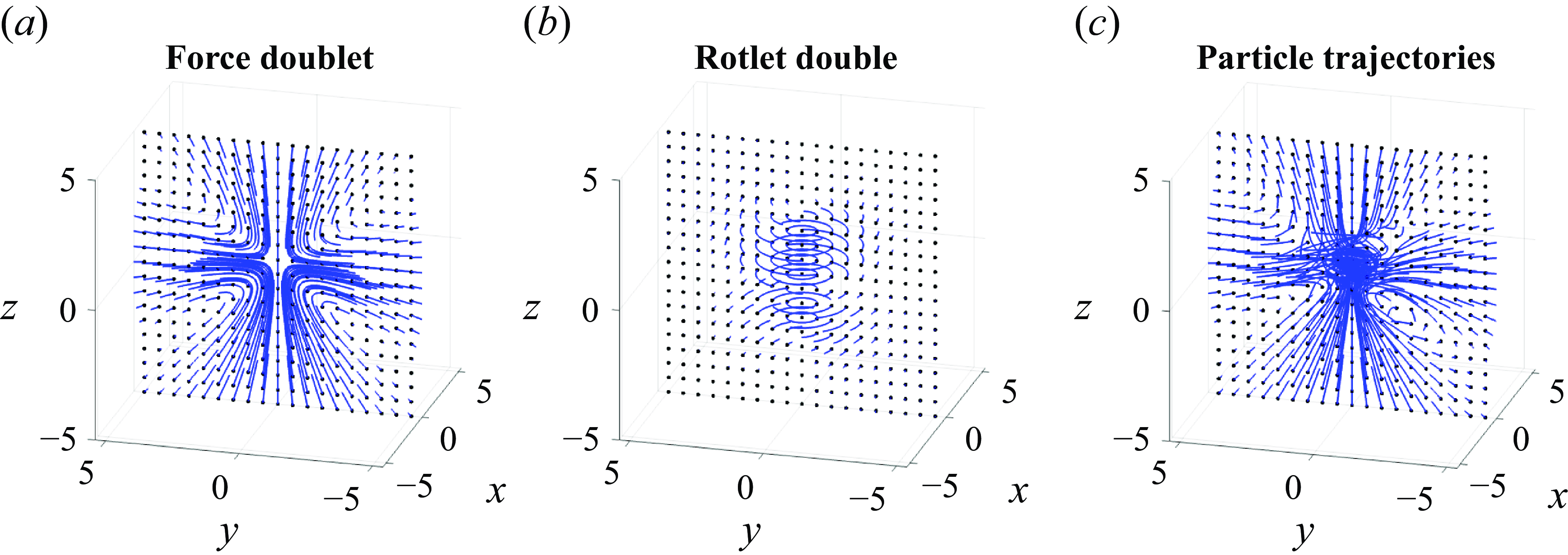
Figure 9. Flow trajectories associated with (a) the force doublet, (b) the rotlet double and (c) their combined contributions, given $q_0=-4\pi$
,
$q_0=-4\pi$
, $b_0=q_0/2$
,
$b_0=q_0/2$
, $q_0^{r}=2\pi$
,
$q_0^{r}=2\pi$
, $C_{r}=-1$
and
$C_{r}=-1$
and $\epsilon =1$
.
$\epsilon =1$
.
3.4. Flows near an infinite plane wall
Swimming microorganisms generally move in confined environments where the fluid motion is affected by the presence of surfaces and other obstacles. In the case of the model presented here, which is derived from regularised Stokeslets, the flows bounded by a plane can be computed using the method of images for regularised elements. We consider a plane wall at $z= z_w$
and the fluid domain to be all points
$z= z_w$
and the fluid domain to be all points $(x,y,z)$
with
$(x,y,z)$
with $z\gt z_w$
. The fluid velocity generated by the swimmers must vanish at the wall. To accomplish this analytically, we define the image of a point
$z\gt z_w$
. The fluid velocity generated by the swimmers must vanish at the wall. To accomplish this analytically, we define the image of a point $(x_0,y_0,z_0)$
in the fluid to be
$(x_0,y_0,z_0)$
in the fluid to be $(x_0, y_0,2z_w-z_0)$
and place regularised singularity solutions of Stokes equations at the image point of a swimmer so that they cancel the flow due to the swimmer at the wall. The formulae for the images of a Stokeslet, a force dipole and for a potential dipole have been derived in Cortez & Varela (Reference Cortez and Varela2015). Here, we present how to use those formulae in the context of the force-doublet swimmer model. Details of the image system used in this section are shown in Appendix B.
$(x_0, y_0,2z_w-z_0)$
and place regularised singularity solutions of Stokes equations at the image point of a swimmer so that they cancel the flow due to the swimmer at the wall. The formulae for the images of a Stokeslet, a force dipole and for a potential dipole have been derived in Cortez & Varela (Reference Cortez and Varela2015). Here, we present how to use those formulae in the context of the force-doublet swimmer model. Details of the image system used in this section are shown in Appendix B.
Given the regularising function
 \begin{equation} \phi _\epsilon (r) = \frac {15 \epsilon ^4}{8\pi (r^2+\epsilon ^2)^{7/2}} ,\end{equation}
the components of velocity from our model are given by (2.7), (2.9) and (2.10)
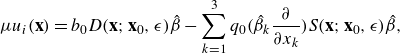 \begin{equation} \mu u_i({\textbf{x}}) = b_0 D({\textbf{x}};{\textbf{x}}_0,\epsilon ) \hat \beta -\sum _{k=1}^3 q_0 \Big (\hat \beta _k \frac {\partial }{\partial x_k} \Big ) S({\textbf{x}};{\textbf{x}}_0,\epsilon )\hat \beta ,\end{equation}
where $S({\textbf{x}};{\textbf{x}}_0,\epsilon )$
is the Stokeslet velocity kernel, and
$S({\textbf{x}};{\textbf{x}}_0,\epsilon )$
is the Stokeslet velocity kernel, and $D({\textbf{x}};{\textbf{x}}_0,\epsilon )$
is the potential dipole kernel. This dipole is derived from a different regularising function, which in Cortez & Varela (Reference Cortez and Varela2015) is called the companion blob, and is used in the image system for a Stokeslet.
$D({\textbf{x}};{\textbf{x}}_0,\epsilon )$
is the potential dipole kernel. This dipole is derived from a different regularising function, which in Cortez & Varela (Reference Cortez and Varela2015) is called the companion blob, and is used in the image system for a Stokeslet.
Figure 10 shows the streamlines resulting from a single organism swimming parallel to a nearby ( $z=0$
) wall (figure 10
a), from a faraway (
$z=0$
) wall (figure 10
a), from a faraway ( $z=-1000$
) wall (figure 10
b), as well as at an angle with respect to a nearby (z = 0) wall (figure 10
c). We note how the inclusion of a nearby wall alters the resulting flow fields, with vortices formed in the region between the swimmer location and the wall. Taking apart the different components of the force-doublet flow field, we plot the contributions of the dipole (figure 10
d) and the stresslet (figure 10
e) of the swimmer in figure 10(a). The resulting flow shows that the symmetry of the stresslet generates two counter-rotating vortices by the edge of the domain and a single vortex due to the inclusion of the dipole, which in turn combine so as to create an asymmetry in the full force-doublet generated flow field. In figure 10(f), we note similarities in the resulting flow profiles of the wall to previous work in Ainley et al. (Reference Ainley, Durkin, Embid, Boindala and Cortez2008), where two regularised Stokeslet particles are used to model a swimmer and placed near a wall, resembling the stresslet component of the force-doublet model.
$z=-1000$
) wall (figure 10
b), as well as at an angle with respect to a nearby (z = 0) wall (figure 10
c). We note how the inclusion of a nearby wall alters the resulting flow fields, with vortices formed in the region between the swimmer location and the wall. Taking apart the different components of the force-doublet flow field, we plot the contributions of the dipole (figure 10
d) and the stresslet (figure 10
e) of the swimmer in figure 10(a). The resulting flow shows that the symmetry of the stresslet generates two counter-rotating vortices by the edge of the domain and a single vortex due to the inclusion of the dipole, which in turn combine so as to create an asymmetry in the full force-doublet generated flow field. In figure 10(f), we note similarities in the resulting flow profiles of the wall to previous work in Ainley et al. (Reference Ainley, Durkin, Embid, Boindala and Cortez2008), where two regularised Stokeslet particles are used to model a swimmer and placed near a wall, resembling the stresslet component of the force-doublet model.
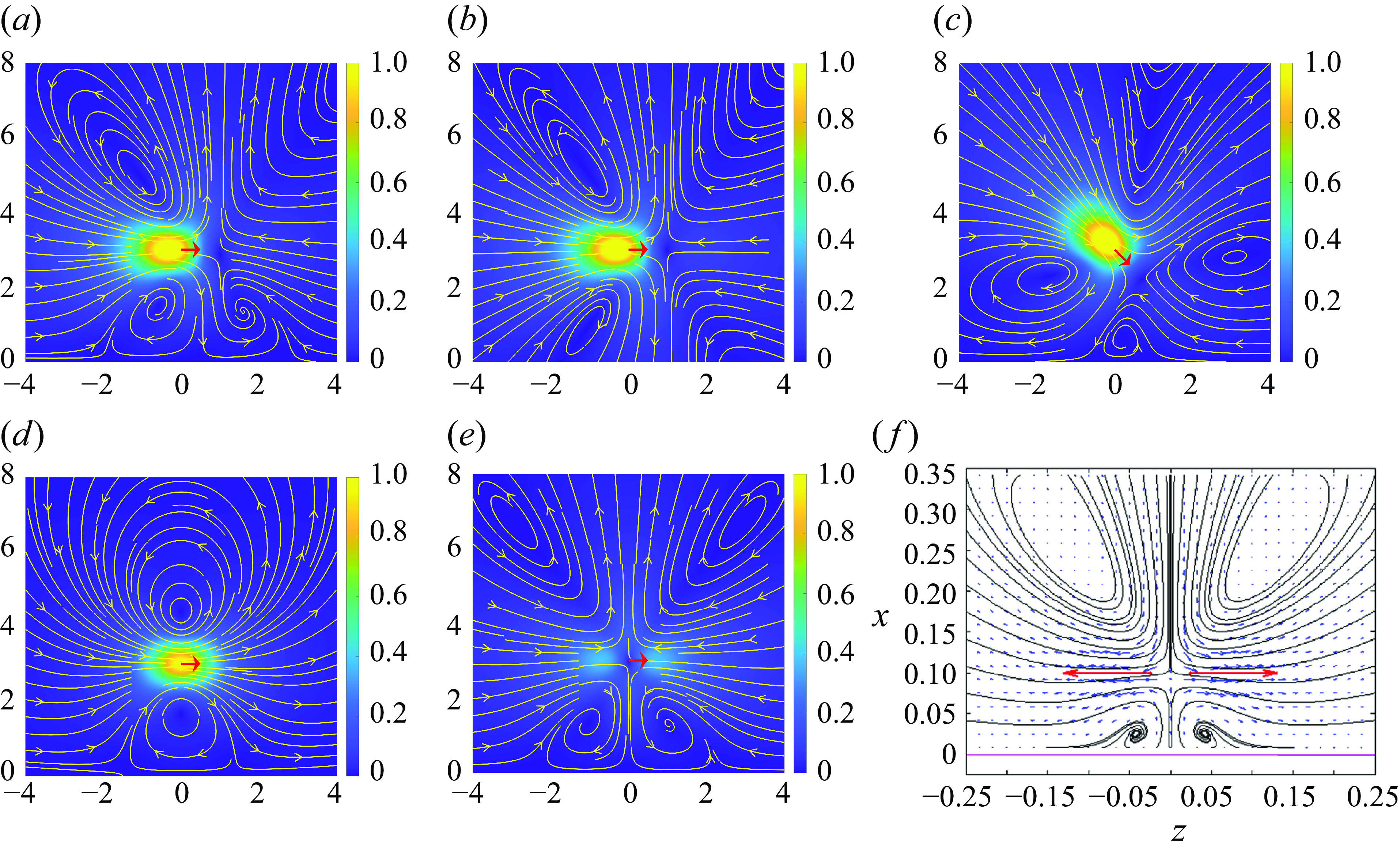
Figure 10. Plots of the velocity streamlines along the centre plane over the scalar field of the velocity magnitude for (a) swimmer by a wall at $z=0$
and (b) the identical swimmer far away from a wall (
$z=0$
and (b) the identical swimmer far away from a wall ( $z=1000$
), (c) a swimmer angled towards the wall a wall at
$z=1000$
), (c) a swimmer angled towards the wall a wall at $z=0$
with
$z=0$
with $\beta =(\sqrt {2}/2,0,-\sqrt {2}/2)$
. Here,
$\beta =(\sqrt {2}/2,0,-\sqrt {2}/2)$
. Here, $q_0=-4\pi$
,
$q_0=-4\pi$
, $b_0=-4\pi$
, and
$b_0=-4\pi$
, and $\epsilon =1.0$
for both simulations with a swimmer centred at
$\epsilon =1.0$
for both simulations with a swimmer centred at $\mathbf {x}=(0,0,3)$
. We plot (d) the dipole and (e) stresslet components of the flows generated by the swimmer in (a). The resulting flows of the stresslet near the wall are comparable to (f) the flow fields of a two-point swimmer described in Ainley et al. (Reference Ainley, Durkin, Embid, Boindala and Cortez2008).
$\mathbf {x}=(0,0,3)$
. We plot (d) the dipole and (e) stresslet components of the flows generated by the swimmer in (a). The resulting flows of the stresslet near the wall are comparable to (f) the flow fields of a two-point swimmer described in Ainley et al. (Reference Ainley, Durkin, Embid, Boindala and Cortez2008).
4. Discussion
In this study, we have presented a mathematical framework for modelling the fluid flows generated by microswimmers in a Stokes fluid. This mathematical framework, the force-doublet framework, uses a reduced, cycle-averaged description of fluid flows generated by microswimmers using a single point particle to encapsulate their resulting fluid flows. This force-doublet approach is derived from taking a limit of a two-point regularised Stokeslet description of the swimmer. The two-point model takes advantage of the method of regularised Stokeslets’ regularisation parameter to account for the asymmetry of the flow fields generated by the swimmer’s body and flagellum, allowing us to easily recreate the asymmetries of the pusher and puller fluid dynamics. The derivation of the single point particle in turn reflects this asymmetry with the presence of a stresslet and a potential dipole in the formulation. Furthermore, we have detailed the stability of two swimmers moving in tandem and the resulting stability regions associated both with their orientation and flow field. Finally, we showed the versatility and relative ease of this modelling framework for incorporating other flow characteristics, such as rotational flows generated by the swimmer, by incorporating a rotlet double in the model framework, as well as wall effects, via the method of images.
The velocity expression in our model is a regularised version of the well-known force-dipole model (Lauga & Powers Reference Lauga and Powers2009; Spagnolie & Lauga Reference Spagnolie and Lauga2012; Bárdfalvy et al. Reference Bárdfalvy2024). To see this, we take the limit of the velocity expression (2.10) as $\epsilon \to 0$
. This eliminates the last term on the right since
$\epsilon \to 0$
. This eliminates the last term on the right since $b_0 = C q_0 \epsilon$
. The last term in the stresslet also vanishes and
$b_0 = C q_0 \epsilon$
. The last term in the stresslet also vanishes and $R\to r=|{\textbf{x}}-{\textbf{x}}_0|$
. What remains is
$R\to r=|{\textbf{x}}-{\textbf{x}}_0|$
. What remains is
 \begin{align} {\textbf{u}}({\textbf{x}})= \frac {q_0}{8\pi \mu r^2} \frac {{\textbf{x}}-{\textbf{x}}_0}{ r} \Big( 3 \Big( {\boldsymbol {\beta }}_0\cdot \frac {{\textbf{x}}-{\textbf{x}}_0}{r}\Big)^2 -1 \Big), \end{align}
which is the force-dipole model. In the regularised version, the additional term of the stresslet ensures that the incompressibility condition is satisfied analytically. The model we have derived is similar to the one developed in Delmotte et al. (Reference Delmotte, Keaveny, Plouraboué and Climent2015), although there are some differences and our derivation is completely different. The model developed in Delmotte et al. (Reference Delmotte, Keaveny, Plouraboué and Climent2015) is based on adapting the squirmer model (Lighthill Reference Lighthill1952; Blake Reference Blake1971; Ishikawa et al. Reference Ishikawa, Simmonds and Pedley2006), where a spherical particle with prescribed axisymmetric surface velocity deforms the shape of the boundary to provide motion to the particle, using a force coupling model (Liu et al. Reference Liu, Keaveny, Maxey and Karniadakis2009; Yeo & Maxey Reference Yeo and Maxey2010; Maxey Reference Maxey2017).
Our model also shares features with the work in Ishimoto & Gaffney (Reference Ishimoto and Gaffney2013), Ishimoto et al. (Reference Ishimoto, Gadêlha, Gaffney, Smith and Kirkman-Brown2017, Reference Ishimoto, Gaffney and Walker2020) and Gaffney et al. (Reference Gaffney, Ishimoto and Walker2021). Their model includes two equal and opposite regularised Stokeslets and two equal and opposite regularised rotlets separated by a small distance. The rotlets and Stokeslets are located at the same points, although each one of the four elements has a different regularisation parameter value. In our model, the limiting process results in a force dipole and a potential dipole at a single location (and a single regularisation parameter). As described earlier, rotlets may also be included in our model, which would introduce a rotlet double with its own regularisation parameter. The relatively low number of parameters in the model framework would allow for a similar process of fitting to experimental flow data that was detailed in Ishimoto et al. (Reference Ishimoto, Gaffney and Walker2020).
As discussed in previous sections, the flow generated by an organism described as a pusher typically displays a stagnation point along its axis located slightly behind the cell body near the anterior end of the flagellum. For a puller, the stagnation point is generally located ahead of the cell body, in front of the organism, although this is not necessarily the case throughout all phases of the flagellar beat. Chlamydomonas reinhardtii, for example, exhibits a time-dependent instantaneous flow field in which the stagnation point moves from the back of the cell body to the front during a beat cycle. High-speed imaging measurements (Guasto et al. Reference Guasto, Johnson and Gollub2010) show fluid flow rotations that reverse direction during other phases of the cycle. See also Delmotte et al. (Reference Delmotte, Keaveny, Plouraboué and Climent2015). In the method presented here, the parameters $q_0$
and
$q_0$
and $b_0$
can be time-dependent and tuned to reproduce flows where the stagnation point moves from one side of the cell body to the other.
$b_0$
can be time-dependent and tuned to reproduce flows where the stagnation point moves from one side of the cell body to the other.
We do note that the modelling framework does come with its own inherent limitations. The formulation is intended for capturing far-field, cycle-averaged hydrodynamics of dilute suspensions of swimmers, sacrificing the detail of high-fidelity fully descriptive models for a single-point evaluation. Some additional modification to the model could allow for a time-varying flow field, as opposed to cycle-averaged flows, by fitting the stagnation over a swimming cycle to experimental data (Delmotte et al. Reference Delmotte, Keaveny, Plouraboué and Climent2015; Ishimoto et al. Reference Ishimoto, Gaffney and Walker2020). Additionally, near-field flow characteristics could be further addressed by designing regularising functions that approximate some feature of the near-field flow.
As it stands, the framework derived can be implemented to understand features of collective phenomenon, with the intent of future investigations into many-swimmer interactions and correlations between swimming speed and orientation (Wu & Libchaber Reference Wu and Libchaber2000; Hernandez-Ortiz et al. Reference Hernandez-Ortiz, Stoltz and Graham2005; Mehandia & Nott Reference Mehandia and Nott2008; Lushi & Peskin Reference Lushi and Peskin2013; Schwarzendahl & Mazza Reference Schwarzendahl and Mazza2018, Reference Schwarzendahl and Mazza2019). Bacteria exposed to antibiotics have been shown to modify their colonial structure in order to maximise their survival (Fung et al. Reference Fung, Konkol, Ishikawa, Larson, Brunet and Goldstein2023). They seem to keep track of their past encounters and adapt as a colony, which would require some sort of chemotactic signalling (BenJacob & Levine Reference BenJacob and Levine2006; Ryan Reference Ryan2019). A much more robust model would be one that incorporates the fluid dynamics with regulation of the chemoattractant emission (Eyiyurekli et al. Reference Eyiyurekli, Manley, Lelkes and Breen2008) and optimal tumbling rate (Dillon et al. Reference Dillon, Fauci and Gaver1995; Strong et al. Reference Strong, Freedman, Bialek and Koberle1998). Furthermore, the numerical experiments performed thus far were restricted to a sample of uniform size. But microorganisms are known to have variability in size, which in turn affects their swimming speeds, and in the presence of other surfaces would also affect their orientation (Ishikawa Reference Ishikawa2009). We would like to understand how the induced changes in swimming speed and orientation would also affect cell aggregation and size of the fluid rotations observed.
As demonstrated by this study, the force-doublet model lends itself easily to other extensions in the method of the regularised Stokeslets framework. The role of biofilms and polymer networks (Cogan et al. Reference Cogan, Cortez and Fauci2005; Cogan & Wolgemuth Reference Cogan and Wolgemuth2011) could be investigated with the inclusion of viscoelastic networks in the fluid (Wróbel et al. Reference Wróbel, Cortez and Fauci2014; Schuech et al. Reference Schuech, Cortez and Fauci2022) or using a formulation of the method of regularised Stokeslets for a Brinkman fluid (Cortez et al. Reference Cortez, Cummins, Leiderman and Varela2010; Ho et al. Reference Ho, Leiderman and Olson2019; Nguyen et al. Reference Nguyen, Olson and Leiderman2019). Further study into the interaction and stability of swimmers near a wall (Berke et al. Reference Berke, Turner and Berg2008) can be examined using an image system to account for a boundary, as described in § 3.4 (Ainley et al. Reference Ainley, Durkin, Embid, Boindala and Cortez2008; Cortez & Varela Reference Cortez and Varela2015; Wróbel et al. Reference Wróbel, Cortez, Varela and Fauci2016). Furthermore, if differences due to the regularisation function are small, the method presented here can be extended to include the use of different blob functions.
Funding.
This work was supported by National Science Foundation Grants DMS 1043626 (to R.C.) and DMS 2240770 (to A.P.H.).
Declaration of interests.
The authors report no conflict of interest.
Appendix A. Summary of the model equations
When tracking the dynamics of a force-doublet particle located at ${\textbf{x}}_0$
, we compute its velocity with (2.10) and use (3.5) to include the effect of torques. The particle’s orientation vector
${\textbf{x}}_0$
, we compute its velocity with (2.10) and use (3.5) to include the effect of torques. The particle’s orientation vector $ {\boldsymbol {\beta }}_0$
evolves according to
$ {\boldsymbol {\beta }}_0$
evolves according to
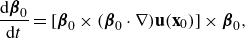 \begin{equation} \frac {\rm d {\boldsymbol {\beta }}_0}{{\rm d}t} = [ {\boldsymbol {\beta }}_0\times ( {\boldsymbol {\beta }}_0\cdot \nabla ){\textbf{u}}({\textbf{x}}_0)]\times {\boldsymbol {\beta }}_0 ,\end{equation}
which requires differentiating the velocity. This velocity may be due to a variety of elements in the fluid, such as Stokeslets due to forces exerted by other organisms nearby, force doublets due to other particles or rotlet doubles due to torques by rotating flagella of other particles. Here, we provide the formulae for the velocity gradients due to regularised Stokeslets, force doublets and rotlets. The derivation of the expressions is based on the regularisation function in (2.3) and uses the diagram in figure 11.
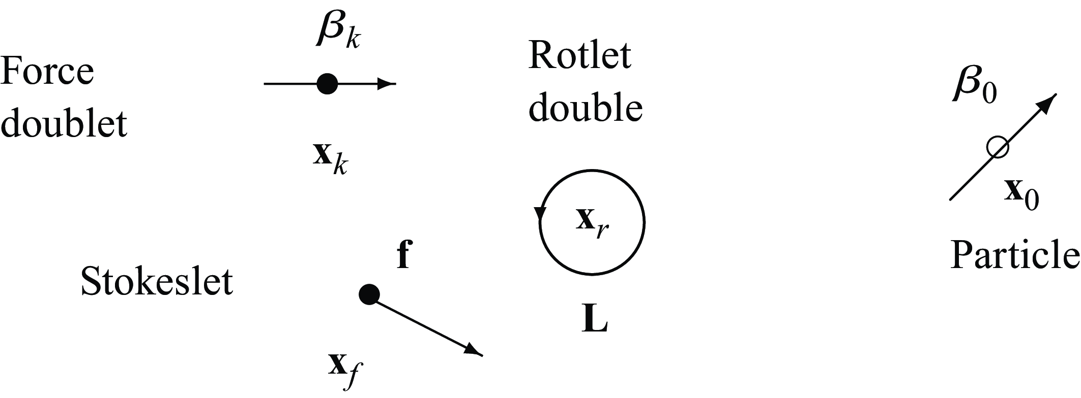
Figure 11. Example of a force-doublet particle located at ${\textbf{x}}_0$
with orientation vector
${\textbf{x}}_0$
with orientation vector $ {\boldsymbol {\beta }}_0$
. The vector
$ {\boldsymbol {\beta }}_0$
. The vector $ {\boldsymbol {\beta }}_0$
will rotate according to (A1) due to the velocity gradients produced by a different force-doublet particle located at
$ {\boldsymbol {\beta }}_0$
will rotate according to (A1) due to the velocity gradients produced by a different force-doublet particle located at ${\textbf{x}}_k$
with orientation vector
${\textbf{x}}_k$
with orientation vector $ {\boldsymbol {\beta }}_k$
, due to a force
$ {\boldsymbol {\beta }}_k$
, due to a force $\textbf{f}$
located at
$\textbf{f}$
located at ${\textbf{x}}_f$
, and due to a rotlet double of strength
${\textbf{x}}_f$
, and due to a rotlet double of strength $\textbf { L} = q_0^r {\boldsymbol {\beta }}$
at
$\textbf { L} = q_0^r {\boldsymbol {\beta }}$
at ${\textbf{x}}_r$
.
${\textbf{x}}_r$
.
A.1 Addition of rotlet doubles
The complete formulation, with rotlet doubles, is as follows:
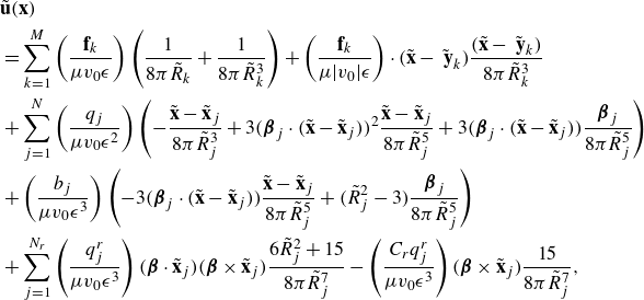 \begin{align} &\tilde {\textbf{u}}({\textbf{x}}) \nonumber\\&= \sum _{k=1}^M \left ( \frac {{\textbf{f}}_k}{\mu v_0\epsilon } \right ) \left ( \frac {1}{8\pi \tilde R_k}+\frac {1}{ 8\pi \tilde R_k^3} \right ) + \left ( \frac {{\textbf{f}}_k}{\mu |v_0|\epsilon } \right ) \cdot (\tilde {\textbf{x}}-\tilde {\textbf { y}}_k) \frac {(\tilde {\textbf{x}}-\tilde {\textbf { y}}_k)}{ 8\pi \tilde R_k^3} \nonumber \\ & + \sum _{j=1}^N \left ( \frac {q_j }{\mu v_0 \epsilon ^2} \right ) \left ( - \frac {\tilde {\textbf{x}}-\tilde {\textbf{x}}_j}{ 8\pi \tilde R_j^3} + 3 ( {\boldsymbol {\beta }}_j\cdot (\tilde {\textbf{x}}-\tilde {\textbf{x}}_j))^2 \frac {\tilde {\textbf{x}}-\tilde {\textbf{x}}_j}{ 8\pi \tilde R_j^5} + 3( {\boldsymbol {\beta }}_j\cdot (\tilde {\textbf{x}}-\tilde {\textbf{x}}_j)) \frac { {\boldsymbol {\beta }}_j}{ 8\pi \tilde R_j^5} \right ) \nonumber \\ &+ \left ( \frac {b_j }{ \mu v_0 \epsilon ^3} \right ) \left ( - 3( {\boldsymbol {\beta }}_j\cdot (\tilde {\textbf{x}}-\tilde {\textbf{x}}_j)) \frac {\tilde {\textbf{x}}-\tilde {\textbf{x}}_j}{ 8\pi \tilde R_j^5} + \big ( \tilde R_j^2-3 \big ) \frac { {\boldsymbol {\beta }}_j}{ 8\pi \tilde R_j^5} \right )\nonumber \\ &+ \sum _{j=1}^{N_r}\left ( \frac {q^r_j }{ \mu v_0 \epsilon ^3} \right ) ( {\boldsymbol {\beta }}\cdot \tilde {\textbf{x}}_j)( {\boldsymbol {\beta }}\times \tilde {\textbf{x}}_j)\frac {6\tilde R_j^2+15}{8\pi \tilde R_j^7} - \left ( \frac {C_r q_j^r}{\mu v_0 \epsilon ^3} \right ) ( {\boldsymbol {\beta }}\times \tilde {\textbf{x}}_j ) \frac {15}{8\pi \tilde R_j^7} ,\end{align}
with the additional dimensionless coefficient associated with the rotlet double
 \begin{equation} \tilde {q}_{j}^{r}=\frac {q_{j}^{r}}{\mu v_0\epsilon ^3}, \end{equation}
using the characteristic quantities of § 2.3.
A.2 The velocity gradient due to a force
We consider a force $\textbf{f}$
located at
$\textbf{f}$
located at ${\textbf{x}}_f$
and let
${\textbf{x}}_f$
and let ${\textbf{x}} = {\textbf{x}}_0-{\textbf{x}}_f$
and
${\textbf{x}} = {\textbf{x}}_0-{\textbf{x}}_f$
and $R^2=\|{\textbf{x}}\|^2+\epsilon ^2$
. The fluid velocity that the force produces at
$R^2=\|{\textbf{x}}\|^2+\epsilon ^2$
. The fluid velocity that the force produces at ${\textbf{x}}_0$
given in (2.4) can be written as
${\textbf{x}}_0$
given in (2.4) can be written as
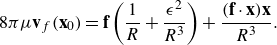 \begin{equation} 8\pi \mu\textbf{v}_f({\textbf{x}}_0) = {\textbf{f}} \left ( \frac {1}{ R}+\frac {\epsilon ^2}{ R^3} \right ) + \frac {({\textbf{f}}\cdot {\textbf{x}}) {\textbf{x}}}{ R^3} . \end{equation}
Then, after simplification, we have that
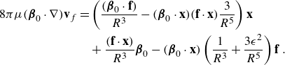 \begin{align} 8\pi \mu ( {\boldsymbol {\beta }}_0\cdot \nabla )\textbf{v}_f &= \left ( \frac { ( {\boldsymbol {\beta }}_0\cdot {\textbf{f}})}{ R^3} - ( {\boldsymbol {\beta }}_0\cdot {\textbf{x}}) ({\textbf{f}}\cdot {\textbf{x}}) \frac {3}{ R^5} \right ) {\textbf{x}}\\&\quad + \frac {({\textbf{f}}\cdot {\textbf{x}})}{ R^3} {\boldsymbol {\beta }}_0 - ( {\boldsymbol {\beta }}_0\cdot {\textbf{x}}) \left ( \frac {1}{ R^3} + \frac {3\epsilon ^2}{ R^5} \right ) {\textbf{f}}\ .\end{align}
We form the cross product $[ {\boldsymbol {\beta }}_0\times ( {\boldsymbol {\beta }}_0\cdot \nabla )\textbf{v}]$
and finally get
$[ {\boldsymbol {\beta }}_0\times ( {\boldsymbol {\beta }}_0\cdot \nabla )\textbf{v}]$
and finally get
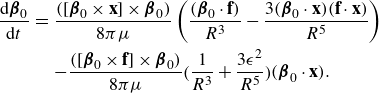 \begin{eqnarray} \frac {\rm d {\boldsymbol {\beta }}_0}{{\rm d}t} &=& \frac {([ {\boldsymbol {\beta }}_0\times {\textbf{x}}]\times {\boldsymbol {\beta }}_0) }{8\pi \mu } \left ( \frac {( {\boldsymbol {\beta }}_0\cdot {\textbf{f}})}{ R^3} - \frac {3( {\boldsymbol {\beta }}_0\cdot {\textbf{x}})({\textbf{f}}\cdot {\textbf{x}}) }{ R^5} \right )\nonumber \\ &&- \frac { ([ {\boldsymbol {\beta }}_0\times {\textbf{f}}]\times {\boldsymbol {\beta }}_0) }{8\pi \mu } \Big ( \frac {1}{ R^3} + \frac {3 \epsilon ^2}{R^5} \Bigr ) ( {\boldsymbol {\beta }}_0\cdot {\textbf{x}}) .\end{eqnarray}
A.3 The velocity gradient due to a force doublet
Consider a force doublet with parameters $q_k$
,
$q_k$
, $b_k$
and orientation vector
$b_k$
and orientation vector $ {\boldsymbol {\beta }}_k$
located at
$ {\boldsymbol {\beta }}_k$
located at ${\textbf{x}}_k$
and let
${\textbf{x}}_k$
and let ${\textbf{x}} = {\textbf{x}}_0-{\textbf{x}}_k$
and
${\textbf{x}} = {\textbf{x}}_0-{\textbf{x}}_k$
and $R^2=\|{\textbf{x}}\|^2+\epsilon ^2$
. The velocity it induces at
$R^2=\|{\textbf{x}}\|^2+\epsilon ^2$
. The velocity it induces at ${\textbf{x}}_0$
is
${\textbf{x}}_0$
is
 \begin{align} {\textbf{u}}({\textbf{x}}_0)= \frac {q_k}{8\pi \mu } \left ( - \frac {{\textbf{x}}}{R^3} + 3 ( {\boldsymbol {\beta }}_k\cdot {\textbf{x}})^2 \frac {{\textbf{x}}}{R^5} + 3( {\boldsymbol {\beta }}_k\cdot {\textbf{x}}) \epsilon ^2 \frac { {\boldsymbol {\beta }}_k}{R^5} \right ) + \frac {b_k }{ 8\pi \mu } D({\textbf{x}}_0;{\textbf{x}}_k,\epsilon ) , \end{align}
where
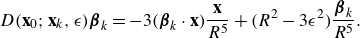 \begin{align} D({\textbf{x}}_0;{\textbf{x}}_k,\epsilon ) {\boldsymbol {\beta }}_k = - 3( {\boldsymbol {\beta }}_k\cdot {\textbf{x}}) \frac {{\textbf{x}}}{ R^5} + \big ( R^2-3\epsilon ^2 \big ) \frac { {\boldsymbol {\beta }}_k}{ R^5} . \end{align}
Then, after simplification, we have that
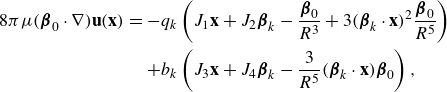 \begin{eqnarray} 8\pi \mu ( {\boldsymbol {\beta }}_0\cdot \nabla ) {\textbf{u}}({\textbf{x}}) &=& - {q_k} \left ( J_1 {\textbf{x}} + J_2 {\boldsymbol {\beta }}_k - \frac { {\boldsymbol {\beta }}_0}{R^3} + 3( {\boldsymbol {\beta }}_k\cdot {\textbf{x}})^2 \frac { {\boldsymbol {\beta }}_0}{R^5} \right ) \nonumber \\ &&+ {b_k} \left ( J_3 {\textbf{x}} + J_4 {\boldsymbol {\beta }}_k -\frac {3}{R^5} ( {\boldsymbol {\beta }}_k\cdot {\textbf{x}}) {\boldsymbol {\beta }}_0 \right ) ,\end{eqnarray}
where
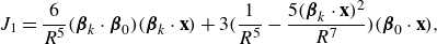 \begin{align} J_1 &= \frac {6}{R^5}( {\boldsymbol {\beta }}_k\cdot {\boldsymbol {\beta }}_0) ( {\boldsymbol {\beta }}_k\cdot {\textbf{x}}) + 3 \Big ( \frac {1}{R^5} - \frac { 5 ( {\boldsymbol {\beta }}_k\cdot {\textbf{x}})^2 }{R^7} \Big ) ( {\boldsymbol {\beta }}_0\cdot {\textbf{x}}), \end{align}
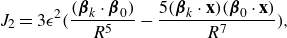 \begin{align} J_2 &= 3 \epsilon ^2 \Big (\frac {( {\boldsymbol {\beta }}_k\cdot {\boldsymbol {\beta }}_0) }{R^5} - \frac { 5( {\boldsymbol {\beta }}_k\cdot {\textbf{x}}) ( {\boldsymbol {\beta }}_0\cdot {\textbf{x}}) }{R^7} \Big ), \end{align}
 \begin{align} J_3 &= -\frac {3}{R^5} ( {\boldsymbol {\beta }}_k\cdot {\boldsymbol {\beta }}_0) + \frac {15}{R^7} ( {\boldsymbol {\beta }}_k\cdot {\textbf{x}}) ( {\boldsymbol {\beta }}_0\cdot {\textbf{x}}) ,\end{align}
 \begin{align} J_4 &= \left( -\frac {3}{R^5} + \epsilon ^2 \frac {15}{R^7} \right) ( {\boldsymbol {\beta }}_0\cdot {\textbf{x}}) .\end{align}
We form the cross-product $[ {\boldsymbol {\beta }}_0\times ( {\boldsymbol {\beta }}_0\cdot \nabla )\textbf{v}]$
and finally get
$[ {\boldsymbol {\beta }}_0\times ( {\boldsymbol {\beta }}_0\cdot \nabla )\textbf{v}]$
and finally get
 \begin{eqnarray} \frac {\rm d {\boldsymbol {\beta }}_0}{{\rm d}t} &=& \frac {([ {\boldsymbol {\beta }}_0\times {\textbf{x}}]\times {\boldsymbol {\beta }}_0) }{8\pi \mu } \left ( - {q_k} J_1 + {b_k} J_3 \right )\nonumber \\ &&+ \frac { ([ {\boldsymbol {\beta }}_0\times {\boldsymbol {\beta }}_k]\times {\boldsymbol {\beta }}_0) }{8\pi \mu } ( - {q_k} J_2 + {b_k} J_4 ). \end{eqnarray}
A.4 The velocity gradient due to a rotlet double
We consider a rotlet double of strength $q_0^r {\boldsymbol {\beta }}$
located at
$q_0^r {\boldsymbol {\beta }}$
located at ${\textbf{x}}_r$
and let
${\textbf{x}}_r$
and let ${\textbf{x}} = {\textbf{x}}_0-{\textbf{x}}_r$
and
${\textbf{x}} = {\textbf{x}}_0-{\textbf{x}}_r$
and $R^2=\|{\textbf{x}}\|^2+\epsilon ^2$
. The fluid velocity that the rotlet double produces at
$R^2=\|{\textbf{x}}\|^2+\epsilon ^2$
. The fluid velocity that the rotlet double produces at ${\textbf{x}}_0$
can be written as
${\textbf{x}}_0$
can be written as
 \begin{equation} 8\pi \mu\textbf{v}_r({\textbf{x}}_0) = q_0^r ( {\boldsymbol {\beta }}\cdot \mathbf {x})( {\boldsymbol {\beta }}\times \mathbf {x})\frac {6R^2+15\epsilon ^2}{ R^7} - C_r q_0^r ( {\boldsymbol {\beta }}\times {\textbf{x}} ) \frac {15\epsilon ^3}{ R^7} ,\end{equation}
where $C_r$
is an asymmetry parameter. Then, after simplification, we have that
$C_r$
is an asymmetry parameter. Then, after simplification, we have that
 \begin{eqnarray} 8\pi \mu ( {\boldsymbol {\beta }}_0\cdot \nabla )\textbf{v}_r &=& q_0^r ( ( {\boldsymbol {\beta }}\times {\boldsymbol {\beta }}_0) ( {\boldsymbol {\beta }}\cdot {\textbf{x}}) + ( {\boldsymbol {\beta }}_0\cdot {\boldsymbol {\beta }}) ( {\boldsymbol {\beta }}\times {\textbf{x}}) ) \Big (\frac {6}{R^5}+ \frac {15\epsilon ^2}{ R^7}\Big )\nonumber \\ &&- q_0^r ( {\boldsymbol {\beta }}\cdot {\textbf{x}}) ( {\boldsymbol {\beta }}_0\cdot {\textbf{x}}) ( {\boldsymbol {\beta }}\times {\textbf{x}}) \Big (\frac {30}{R^7}+\frac {105\epsilon ^2}{ R^9} \Big ) \nonumber \\ &&+C_r q_0^r \Big ( \frac {105\epsilon ^3}{ R^9}( {\boldsymbol {\beta }}_0\cdot {\textbf{x}})\ ( {\boldsymbol {\beta }}\times {\textbf{x}}) -\frac {15\epsilon ^3}{ R^7} ( {\boldsymbol {\beta }}\times {\boldsymbol {\beta }}_0) \Big ) .\end{eqnarray}
We form the cross product $[ {\boldsymbol {\beta }}_0\times ( {\boldsymbol {\beta }}_0\cdot \nabla )\textbf{v}]$
and finally get
$[ {\boldsymbol {\beta }}_0\times ( {\boldsymbol {\beta }}_0\cdot \nabla )\textbf{v}]$
and finally get
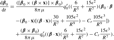 \begin{eqnarray} \frac {\rm d {\boldsymbol {\beta }}_0}{{\rm d}t} &=& \frac {([ {\boldsymbol {\beta }}_0\times ( {\boldsymbol {\beta }}\times {\textbf{x}})]\times {\boldsymbol {\beta }}_0) }{8\pi \mu } q_0^r \Big ( \Big (\frac {6}{R^5} + \frac {15\epsilon ^2}{ R^7}\Big ) ( {\boldsymbol {\beta }}_0\cdot {\boldsymbol {\beta }} \nonumber \\ &&- ( {\boldsymbol {\beta }}_0\cdot {\textbf{x}}) \Big [ ( {\boldsymbol {\beta }}\cdot {\textbf{x}}) \Big (\frac {30}{R^7}+\frac {105\epsilon ^2}{ R^9} \Big ) - C_r \frac {105\epsilon ^3}{ R^9} \Big ] \Big ) \nonumber \\ &&+ \frac { ( {\boldsymbol {\beta }}\times {\boldsymbol {\beta }}_0) }{8\pi \mu } q_0^r \Big ( ( {\boldsymbol {\beta }}\cdot {\textbf{x}}) \Big (\frac {6}{R^5} + \frac {15\epsilon ^2}{ R^7}\Big ) - C_r \frac {15\epsilon ^3}{ R^7} \Bigr ). \end{eqnarray}
Appendix B. Method of images for force doublets
Here, we briefly describe and provide the formulae for the flow in the half-space $y_3\gt 0$
generated by a force doublet located at
$y_3\gt 0$
generated by a force doublet located at $\textbf{y}$
. We assume that
$\textbf{y}$
. We assume that $y_3 = h$
, so that
$y_3 = h$
, so that $h$
is the distance from the swimmer to the wall. The plane
$h$
is the distance from the swimmer to the wall. The plane $y_3=0$
is considered a solid wall where the fluid velocity must be zero. This is accomplished by computing the flow due to the force doublet at
$y_3=0$
is considered a solid wall where the fluid velocity must be zero. This is accomplished by computing the flow due to the force doublet at $\textbf{y}$
and adding to it the flow generated by several regularised elements centred at the image point
$\textbf{y}$
and adding to it the flow generated by several regularised elements centred at the image point $\textbf{y}^{IM} = (y_1, y_2, -y_3)$
so that the combination of the velocities due to all elements is analytically zero at all points of the wall.
$\textbf{y}^{IM} = (y_1, y_2, -y_3)$
so that the combination of the velocities due to all elements is analytically zero at all points of the wall.
In this appendix, we use the notation ${\textbf{x}}_e$
to denote the point where the velocity is evaluated and
${\textbf{x}}_e$
to denote the point where the velocity is evaluated and ${\textbf{x}} = {\textbf{x}}_e-\textbf{y}^{IM}$
. Also,
${\textbf{x}} = {\textbf{x}}_e-\textbf{y}^{IM}$
. Also, $r^2 = |{\textbf{x}}|^2 = x_j x_j$
(summation over repeated indices is implied), and we let
$r^2 = |{\textbf{x}}|^2 = x_j x_j$
(summation over repeated indices is implied), and we let $R^2=r^2+\epsilon ^2$
. The orientation vector of the force doublet is
$R^2=r^2+\epsilon ^2$
. The orientation vector of the force doublet is $\hat \beta$
and the vector
$\hat \beta$
and the vector $\textbf { g} = (\hat \beta _1,\hat \beta _2,-\hat \beta _3)$
. Define the functions
$\textbf { g} = (\hat \beta _1,\hat \beta _2,-\hat \beta _3)$
. Define the functions
 \begin{align} \psi (r) = \frac {15 \epsilon ^4}{8\pi R^7}, \ \ \ \ \ H_2(r) = \frac {1}{8\pi R^3}, \ \ \ \ \ H_1(r) = \epsilon ^2 H_2 + \frac {1}{8\pi R}, \\[-24pt] \nonumber \end{align}
 \begin{align} \phi (r) = \frac {6 \epsilon ^2}{8\pi R^5}, \ \ \ \ \ D_2(r) = \frac {6}{8\pi R^5}, \ \ \ \ \ D_1(r) = \epsilon ^2 D_2 - \frac {2}{8\pi R^3}, \ \ \ \ \ \ J_2(r) = \frac {D'_2}{R} , \end{align}
and define the regularised Green’s functions as the solutions of $\triangle G_s = \psi$
and
$\triangle G_s = \psi$
and $\triangle G_d = \phi$
.
$\triangle G_d = \phi$
.
The Stokeslet and potential dipole kernels in component form are
 \begin{align} S_{ij} = H_1(r) \delta _{ij} + H_2(r) x_i x_j ,\end{align}
 \begin{align} D_{ij} = D_1(r) \delta _{ij} + D_2(r) x_i x_j. \end{align}
The force-doublet velocity is a linear combination of a stresslet and a potential dipole, as described in (2.8)
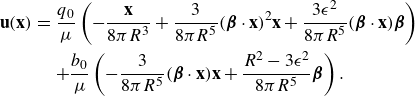 \begin{eqnarray} {\textbf{u}}({\textbf{x}}) &=& \frac {q_0}{\mu } \left ( - \frac {{\textbf{x}}}{8\pi R^3} + \frac {3}{8\pi R^5}( {\boldsymbol {\beta }}\cdot {\textbf{x}})^2{\textbf{x}} + \frac {3\epsilon ^2}{8\pi R^5}( {\boldsymbol {\beta }}\cdot {\textbf{x}}) {\boldsymbol {\beta }} \right )\nonumber \\ &&+ \frac {b_0 }{\mu } \left ( -\frac {3}{8\pi R^5}( {\boldsymbol {\beta }}\cdot {\textbf{x}}){\textbf{x}} + \frac {R^2-3\epsilon ^2}{8\pi R^5} {\boldsymbol {\beta }} \right ). \end{eqnarray}
To work with the images, we write this expression in terms of the functions defined above
 \begin{align} {\textbf{u}}({\textbf{x}}) = -\frac {q_0}{\mu } ( {\boldsymbol {\beta }}\cdot \nabla ) \left ( H_2 ( {\boldsymbol {\beta }}\cdot {\textbf{x}}){\textbf{x}} + H_1 {\boldsymbol {\beta }} \right ) - \frac {b_0 }{2\mu } \left ( D_2 ( {\boldsymbol {\beta }}\cdot {\textbf{x}}){\textbf{x}} + D_1 {\boldsymbol {\beta }} \right ) .\end{align}
The image system for each of these elements is given in Cortez & Varela (Reference Cortez and Varela2015). The image system for $( {\boldsymbol {\beta }}\cdot \nabla ) ( H_2 ( {\boldsymbol {\beta }}\cdot {\textbf{x}}){\textbf{x}} + H_1 {\boldsymbol {\beta }} )$
can be summarised as
$( {\boldsymbol {\beta }}\cdot \nabla ) ( H_2 ( {\boldsymbol {\beta }}\cdot {\textbf{x}}){\textbf{x}} + H_1 {\boldsymbol {\beta }} )$
can be summarised as
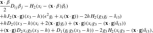 \begin{eqnarray} && \frac {{\textbf{x}}\cdot \beta }{2} D_{ij} \beta _j - H_2(x_i - ({\textbf{x}}\cdot \beta ) \beta _i ) \nonumber \\ && + h J_2 ({\textbf{x}}\cdot\textbf{g}) (x_3 -h) ( \epsilon ^2 g_{i} + x_i ({\textbf{x}}\cdot\textbf{g}) ) - 2h H_2 ( g_3 g_i - \delta _{i3}) \nonumber \\ && + h D_2 ( (x_3-h) (x_i + 2 ({\textbf{x}}\cdot\textbf{g}) g_{i}) + ({\textbf{x}}\cdot\textbf{g}) ( x_i g_{3} - ({\textbf{x}}\cdot\textbf{g}) \delta _{i3} ) ) \nonumber \\ &&+ ({\textbf{x}}\cdot\textbf{g}) D_2 x_{i} g_3 (x_3-h) + D_1 (g_{i} g_3 (x_3-h) ) - 2 g_3 H_2 ( x_i g_{3} - ({\textbf{x}}\cdot\textbf{g}) \delta _{i3} ) ,\end{eqnarray}
where ${\textbf{x}} = {\textbf{x}}_e -\textbf{y}^{IM}$
and
${\textbf{x}} = {\textbf{x}}_e -\textbf{y}^{IM}$
and ${\textbf{x}}_e$
is the point where the velocity is evaluated.
${\textbf{x}}_e$
is the point where the velocity is evaluated.
The image system for the potential dipole $D_2 ( {\boldsymbol {\beta }}\cdot {\textbf{x}}){\textbf{x}} + D_1 {\boldsymbol {\beta }}$
is
$D_2 ( {\boldsymbol {\beta }}\cdot {\textbf{x}}){\textbf{x}} + D_1 {\boldsymbol {\beta }}$
is
 \begin{eqnarray} D^{IM}_{ik} \hat \beta _k &=& D^*_{ik} \hat \beta _k- D_{ik} \hat \beta _k-2D_2 x_3 (x_i g_{3}-(x\cdot g)\delta _{i3} ) + 2 (h-x_3) Q_{in3} g_n ,\end{eqnarray}
with
 \begin{align} Q_{in3} g_n = \Big ( D_2 g_3 + J_2 x_3 ({\textbf{x}}\cdot\textbf{g}) \Big ) x_i + D_2 ({\textbf{x}}\cdot\textbf{g}) \delta _{i3} + (D_2 + \epsilon ^2 J_2) x_3 g_i . \end{align}


 Open access