


1. Introduction
We consider dynamical systems whose state  $\pmb {x}$ evolves over a state space $\varOmega \subseteq \mathbb {R}^d$ in discrete time steps according to a function $F:\varOmega \rightarrow \varOmega$. That is,
 \begin{equation} \pmb{x}_{n+1} = F(\pmb{x}_n), \quad n\geq 0,\end{equation}
for an initial state  $\pmb {x}_0$. At the $n$th time step the system is in state $\pmb {x}_{n}$, and such a dynamical system forms a trajectory of iterates $\pmb {x}_0, \pmb {x}_1, \pmb {x}_2,\ldots$ in $\varOmega$. We consider the discrete-time setting since we are interested in analysing data collected from experiments and numerical simulations, where we cannot practically obtain a continuum of data. The dynamical system in (1.1) could, for example, be experimental fluid flow measured in a particle image velocimetry (PIV) window over a grid of discrete spatial points (see § 7 for an example). In that case, the function $F$ corresponds to evolving the flow one time step forward and can, of course, be nonlinear.
Koopman operators (Koopman Reference Koopman1931; Koopman & von Neumann Reference Koopman and von Neumann1932) provide a ‘linearisation’ of nonlinear dynamical systems (1.1) (Mezić Reference Mezić2021). Sparked by Mezić (Reference Mezić2005) and Mezić & Banaszuk (Reference Mezić and Banaszuk2004), recent attention has shifted to using Koopman operators in data-driven methods for studying dynamical systems from trajectory data (Brunton et al. Reference Brunton, Budišić, Kaiser and Kutz2022). The ensuing explosion in popularity, dubbed ‘Koopmanism’ (Budišić, Mohr & Mezić Reference Budišić, Mohr and Mezić2012), includes thousands of articles over the last decade. The Koopman operator for the system (1.1),  $\mathcal {K}$, is defined by its action on ‘observables’ or functions $g:\varOmega \rightarrow \mathbb {C}$, via the composition formula
 \begin{equation} \mathcal{K}g =g\circ F, \quad g\in \mathcal{D}(\mathcal{K}),\end{equation}
where  $\mathcal {D}(\mathcal {K})$ is a suitable domain of observables. Note that observables typically differ from the full state of the system in that they are only a given measure of the system. For example, an observable $g(\pmb {x})$ could be the PIV-measured horizontal fluid velocity at a single point, whereas $\pmb {x}$ could correspond to the velocity values at all spatial grid points at a given time. When applied to a state of the system
 \begin{equation} [\mathcal{K}g] (\pmb{x}_{n})=g(F (\pmb{x}_{n})) = g(\pmb{x}_{n+1}). \end{equation}
Thus,  $\mathcal {K}$ acts on observables by advancing them one step forward in time. By considering $g_j(\pmb {x})=[\pmb {x}]_j$ for $j=1,\ldots , d$, we see that $\mathcal {K}$ encodes the action of $F$ on $\pmb {x}_{n}$. Nevertheless, from (1.2), one can show that $\mathcal {K}$ is a linear operator, regardless of whether the dynamics are linear or nonlinear.
The Koopman operator transforms the nonlinear dynamics in the state variable  $\pmb {x}$ into an equivalent linear dynamics in the observables $g$. Hence, the spectral information of $\mathcal {K}$ determines the behaviour of the dynamical system (1.1). For example, Koopman modes are projections of the physical field onto eigenfunctions of the Koopman operator. For fluid flows, Koopman modes provide collective motions of the fluid that are occurring at the same spatial frequency, growth or decay rate, according to an (approximate) eigenvalue of the Koopman operator. Since the vast majority of turbulent fluid interactions have nonlinear properties, this ability to transition to a linear operator is exceedingly useful. For example, obtaining linear representations for nonlinear systems has the potential to revolutionise our ability to predict and control such systems. However, there is price to pay for this linearisation – $\mathcal {K}$ acts on an infinite-dimensional space, and this is where computational difficulties arise.
In the data-driven setting of this paper, we do not assume knowledge of the function  $F$ in (1.1). Instead, we aim to recover the spectral properties of $\mathcal {K}$ from measured trajectory data. The leading numerical algorithm used to approximate $\mathcal {K}$ from trajectory data is dynamic mode decomposition (DMD) (Tu et al. Reference Tu, Rowley, Luchtenburg, Brunton and Kutz2014; Kutz et al. Reference Kutz, Brunton, Brunton and Proctor2016a). First introduced by Schmid (Reference Schmid2009, Reference Schmid2010) in the fluids community and connected to the Koopman operator in Rowley et al. (Reference Rowley, Mezić, Bagheri, Schlatter and Henningson2009), there are now numerous extensions and variants of DMD (Chen, Tu & Rowley Reference Chen, Tu and Rowley2012; Wynn et al. Reference Wynn, Pearson, Ganapathisubramani and Goulart2013; Jovanović, Schmid & Nichols Reference Jovanović, Schmid and Nichols2014; Kutz, Fu & Brunton Reference Kutz, Fu and Brunton2016b; Noack et al. Reference Noack, Stankiewicz, Morzyński and Schmid2016; Proctor, Brunton & Kutz Reference Proctor, Brunton and Kutz2016; Korda & Mezić Reference Korda and Mezić2018; Loiseau & Brunton Reference Loiseau and Brunton2018; Deem et al. Reference Deem, Cattafesta, Hemati, Zhang, Rowley and Mittal2020; Klus et al. Reference Klus, Nüske, Peitz, Niemann, Clementi and Schütte2020; Baddoo et al. Reference Baddoo, Herrmann, McKeon, Kutz and Brunton2021, Reference Baddoo, Herrmann, McKeon and Brunton2022; Herrmann et al. Reference Herrmann, Baddoo, Semaan, Brunton and McKeon2021; Wang & Shoele Reference Wang and Shoele2021; Colbrook Reference Colbrook2022). Of particular interest is extended DMD (EDMD) (Williams, Kevrekidis & Rowley Reference Williams, Kevrekidis and Rowley2015a), which generalised DMD to a broader class of nonlinear observables. The reader is encouraged to consult Schmid (Reference Schmid2022) for a recent overview of DMD-type methods, and Taira et al. (Reference Taira, Brunton, Dawson, Rowley, Colonius, McKeon, Schmidt, Gordeyev, Theofilis and Ukeiley2017, Reference Taira, Hemati, Brunton, Sun, Duraisamy, Bagheri, Dawson and Yeh2020) and Towne, Schmidt & Colonius (Reference Towne, Schmidt and Colonius2018) for an overview of modal-decomposition techniques in fluid flows. DMD breaks apart a high-dimensional spatio-temporal signal into a triplet of Koopman modes, scalar amplitudes and purely temporal signals. This decomposition allows the user to describe complex flow patterns by a hierarchy of simpler processes. When linearly superimposed, these simpler processes approximately recover the full flow.
DMD is undoubtedly a powerful data-driven algorithm that has led to rapid progress over the past decade (Grilli et al. Reference Grilli, Schmid, Hickel and Adams2012; Mezić Reference Mezić2013; Motheau, Nicoud & Poinsot Reference Motheau, Nicoud and Poinsot2014; Sarmast et al. Reference Sarmast, Dadfar, Mikkelsen, Schlatter, Ivanell, Sørensen and Henningson2014; Sayadi et al. Reference Sayadi, Schmid, Nichols and Moin2014; Subbareddy, Bartkowicz & Candler Reference Subbareddy, Bartkowicz and Candler2014; Chai, Iyer & Mahesh Reference Chai, Iyer and Mahesh2015; Brunton et al. Reference Brunton, Brunton, Proctor and Kutz2016; Hua et al. Reference Hua, Gunaratne, Talley, Gord and Roy2016; Priebe et al. Reference Priebe, Tu, Rowley and Martín2016; Pasquariello, Hickel & Adams Reference Pasquariello, Hickel and Adams2017; Page & Kerswell Reference Page and Kerswell2018, Reference Page and Kerswell2019, Reference Page and Kerswell2020; Brunton & Kutz Reference Brunton and Kutz2019; Korda, Putinar & Mezić Reference Korda, Putinar and Mezić2020). However, the infinite-dimensional nature of  $\mathcal {K}$ leads to several fundamental challenges. The spectral information of infinite-dimensional operators can be far more complicated and challenging to compute than that of a finite matrix (Ben-Artzi et al. Reference Ben-Artzi, Colbrook, Hansen, Nevanlinna and Seidel2020; Colbrook Reference Colbrook2020). For example, $\mathcal {K}$ can have both discrete and continuous spectra (Mezić Reference Mezić2005). Recently, Colbrook & Townsend (Reference Colbrook and Townsend2021) introduced Residual DMD (ResDMD) aimed at tackling some of the challenges associated with infinite dimensions. The idea of ResDMD is summarised in figure 1 (see § 3). ResDMD is easily used in conjunction with existing DMD methods – it does not require additional data and is no more computationally expensive than EDMD. ResDMD addresses the challenges of:
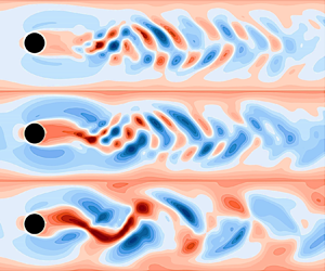
• Spectral pollution (spurious modes). A well-known difficulty of computing spectra of infinite-dimensional operators is spectral pollution, where discretisations to a finite matrix cause the appearance of spurious eigenvalues that have nothing to do with the operator and typically have no physical meaning (Lewin & Séré Reference Lewin and Séré2010; Colbrook, Roman & Hansen Reference Colbrook, Roman and Hansen2019). DMD-type methods typically suffer from spectral pollution and can produce modes with no physical relevance to the system being investigated (Budišić et al. Reference Budišić, Mohr and Mezić2012; Williams et al. Reference Williams, Kevrekidis and Rowley2015a). It is highly desirable to have a principled way of detecting spectral pollution with as few assumptions as possible. By computing residuals associated with the spectrum with error control, ResDMD allows the computation of spectra of general Koopman operators with rigorous convergence guarantees and without spectral pollution. ResDMD verifies computations of spectral properties and provides a data-driven study of dynamical systems with error control (e.g. see Koopman modes in figure 16).
• Invariant subspaces. A finite-dimensional invariant subspace of $\mathcal {K}$ is a space of observables $\mathcal {G} = {\rm span} \{g_1,\ldots,g_k\}$ such that $\mathcal {K}g\in \mathcal {G}$ for all $g\in \mathcal {G}$. Non-trivial finite-dimensional invariant spaces need not exist (e.g. when the system is mixing), can be challenging to compute, or may not capture all of the dynamics of interest. Typically, one must settle for approximate invariant subspaces, and DMD-type methods can result in closure issues (Brunton et al. Reference Brunton, Brunton, Proctor and Kutz2016). By computing upper bounds on residuals, ResDMD provides a way of measuring how invariant a candidate subspace is. It is important to stress that ResDMD computes residuals associated with the underlying infinite-dimensional operator $\mathcal {K}$ (the additional matrix in figure 1 allows us to do this using finite matrices), in contrast to earlier work that computes residuals of observables with respect to a finite DMD discretisation matrix (Drmac, Mezic & Mohr Reference Drmac, Mezic and Mohr2018). In contrast to ResDMD, residuals with respect to a finite DMD discretisation of $\mathcal{K}$ can never be used as error bounds for spectral information of $\mathcal {K}$ and suffer from issues such as spectral pollution. Residuals computed by ResDMD also allow a natural ranking or ordering of approximated eigenvalues and Koopman modes, that can be exploited for efficient system compression (see § 8).
• Continuous spectra. The operator
$\mathcal {K}$ can have a continuous spectrum, which is a generic feature of chaotic or turbulent flow (Basley et al. Reference Basley, Pastur, Lusseyran, Faure and Delprat2011; Arbabi & Mezić Reference Arbabi and Mezić2017b). A formidable challenge is dealing with the continuous spectrum (Mezić Reference Mezić2013; Colbrook Reference Colbrook2021; Colbrook, Horning & Townsend Reference Colbrook, Horning and Townsend2021), since discretising to a finite-dimensional operator destroys its presence. Most existing non-parametric approaches for computing continuous spectra of $\mathcal {K}$ are restricted to ergodic systems (Arbabi & Mezić Reference Arbabi and Mezić2017b; Giannakis Reference Giannakis2019; Korda et al. Reference Korda, Putinar and Mezić2020; Das, Giannakis & Slawinska Reference Das, Giannakis and Slawinska2021), as this allows relevant integrals to be computed using long-time averages. ResDMD (Colbrook & Townsend Reference Colbrook and Townsend2021) provides a general computational framework to deal with continuous spectra through smoothed approximations of spectral measures, leading to explicit and rigorous high-order convergence (see the examples in § 6). The methods deal jointly with discrete and continuous spectra, do not assume ergodicity, and can be applied to data collected from either short or long trajectories.• Nonlinearity and high-dimensional state space. For many fluid flows, e.g. turbulent phenomena, the corresponding dynamical system is strongly nonlinear and has a very large state-space dimension. ResDMD can be combined with learned dictionaries to tackle this issue. A key advantage of ResDMD compared with traditional learning methods is that one still has convergence theory and can perform a posteriori verification that the learned dictionary is suitable. In this paper, we demonstrate this for two choices of dictionary: kernelised extended dynamic mode decomposition (kEDMD) (Williams, Rowley & Kevrekidis Reference Williams, Rowley and Kevrekidis2015b) and (rank-reduced) DMD.


Figure 1. The basic idea of ResDMD – by introducing an additional matrix  $\varPsi _Y^*W\varPsi _Y$ (compared with EDMD), we compute a residual in infinite dimensions. The matrices $\varPsi _X$ and $\varPsi _Y$ are defined in (2.8a,b) and correspond to the dictionary evaluated at the snapshot data. The matrix $W=\mathrm {diag}(w_1,\ldots,w_M)$ is a diagonal weight matrix. The approximation of the residual becomes exact in the large data limit $M\rightarrow \infty$.
This paper demonstrates ResDMD in a wide range of fluid dynamic situations, at varying Reynolds numbers, from both numerical and experimental data. We discuss how the new ResDMD methods can be reliably used for turbulent flows such as aerodynamic boundary layers, and we include, for the first time, a link between the spectral measures of Koopman operators and turbulent power spectra. By windowing in the frequency domain, ResDMD avoids the problem of broadening and also allows convergence theory. We illustrate this link explicitly for experimental measurements of boundary layer turbulence. We also discuss how a new modal ordering based on the residual permits greater accuracy with a smaller DMD dictionary than traditional modal modulus ordering. This result paves the way for greater dynamic compression of large data sets without sacrificing accuracy.
The paper is outlined as follows. In § 2, we recap EDMD, for which DMD is a special case, and interpret the algorithm as a Galerkin method. ResDMD is then introduced in § 3, where we recall and expand upon the results of Colbrook & Townsend (Reference Colbrook and Townsend2021). We stress that ResDMD does not make any assumptions about the Koopman operator or dynamical system. In § 4, we recall one of the algorithms of Colbrook & Townsend (Reference Colbrook and Townsend2021) for computing spectral measures (dealing with continuous spectra) under the assumption that the dynamical system is measure preserving, and make a new link between an algorithm for spectral measures of Koopman operators and the power spectra of signals. We then validate and apply our methods to four different flow cases. We treat flow past a cylinder (numerical data) in § 5, turbulent boundary layer flow (hot-wire experimental data) in § 6, wall-jet boundary layer flow (PIV experimental data) in § 7 and laser-induced plasma (experimental data collected with a microphone) in § 8. In each case, only the flow fields or pressure fields are used to extract relevant dynamical information. We end with a discussion and conclusions in § 9. Code for our methods can be found at https://github.com/MColbrook/Residual-Dynamic-Mode-Decomposition, and we provide a diagrammatic chart for implementation in figure 2.
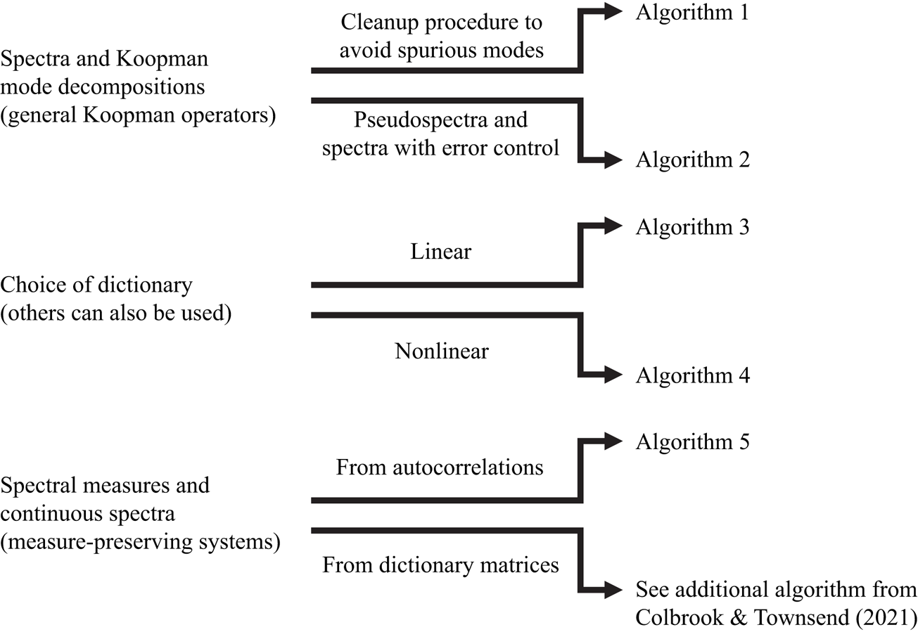
Figure 2. A diagrammatic chart for the algorithms used in this paper. The computational problem is shown on the left, and the relevant algorithms on the right.
2. Recalling DMD
Here, we recall the definition of EDMD from Williams et al. (Reference Williams, Kevrekidis and Rowley2015a) and its interpretation as a Galerkin method. As a particular case of EDMD, DMD can be interpreted as producing a Galerkin approximation of the Koopman operator using linear basis functions.
2.1. Trajectory data
We assume that (1.1) is observed for  $M_2$ time steps, starting at $M_1$ initial conditions. It is helpful to view the trajectory data as an $M_1\times M_2$ matrix
 \begin{equation} B_{{data}} = \begin{bmatrix} \pmb{x}_0^{(1)} & \cdots & \pmb{x}_{M_2-1}^{(1)}\\ \vdots & \ddots & \vdots \\ \pmb{x}_0^{(M_1)} & \cdots & \pmb{x}_{M_2-1}^{(M_1)}\\ \end{bmatrix}.\end{equation}
Each row of  $B_{{data}}$ corresponds to an observation of a single trajectory of the dynamical system that is witnessed for $M_2$ time steps. In particular, $\pmb {x}_{i+1}^{(j)} = F(\pmb {x}_i^{(j)})$ for $0\leq i\leq M_2-2$ and $1\leq j\leq M_1$. For example, these snapshots could be measurements of unsteady velocity field across $M_1$ initial state configurations. One could therefore use just consider $M_2=2$. One could also consider a single trajectory, $M_1=1$, and large $M_2$. The exact structure depends on the data acquisition method. In general, (2.1) could represent measurements of the velocity along $M_1$ trajectories for $M_2$ time steps, a total of $M_1M_2$ measurements. One can also use our algorithms with data consisting of trajectories of different lengths (i.e. general snapshots).
Letting  $\{\pmb {x}^{(m)}\}_{m=1}^M$ and $\{\pmb {y}^{(m)}\}_{m=1}^M$ be enumerations of the first $M_2-1$ columns and the second to final columns of $B_{{data}}$, respectively, with $M=M_1(M_2-1)$, we can conveniently represent the data as a finite set of $M$ pairs of measurements of the state
 \begin{equation} \{\pmb{x}^{(m)},\pmb{y}^{(m)}\}_{m=1}^M \text{ such that } \pmb{y}^{(m)}=F(\pmb{x}^{(m)}),\quad m=1,\ldots,M. \end{equation}
One could also consider measurements of certain observables  $g, \{g(\pmb {x}^{(m)}),g(\pmb {y}^{(m)})\}_{m=1}^M$, and interpret the following algorithms as such. EDMD provides a way of using these measurements to approximate the operator $\mathcal {K}$ via a matrix $\mathbb {K}\in \mathbb {C}^{N\times N}$.
2.2. Extended DMD
We work in the Hilbert space  $L^2(\varOmega,\omega )$ of square-integrable observables with respect to a positive measure $\omega$ on $\varOmega$. We do not assume that this measure is invariant. A common choice of $\omega$ is the standard Lebesgue measure. This choice is natural for Hamiltonian systems, for which the Koopman operator is unitary on $L^2(\varOmega,\omega )$ (Arnold Reference Arnold1989). Another common choice is for $\omega$ to correspond to an ergodic measure on an attractor (Mezić Reference Mezić2005).
Given a dictionary (a set of basis functions)  $\{\psi _1,\ldots,\psi _{N}\}\subset \mathcal {D}(\mathcal {K})\subseteq L^2(\varOmega,\omega )$ of observables, EDMD constructs a matrix $\mathbb {K}\in \mathbb {C}^{N\times N}$ from the snapshot data (2.2) that approximates $\mathcal {K}$ on the finite-dimensional subspace ${V}_{{N}}=\mathrm {span}\{\psi _1,\ldots,\psi _{N}\}$. The choice of the dictionary is up to the user, with some common hand-crafted choices given in Williams et al. (Reference Williams, Kevrekidis and Rowley2015a, table 1). When the state-space dimension $d$ is large, as in this paper, it is beneficial to use a data-driven dictionary. We discuss this in § 3.3, where we present DMD (Kutz et al. Reference Kutz, Brunton, Brunton and Proctor2016a) and kEDMD (Williams et al. Reference Williams, Rowley and Kevrekidis2015b) in a unified framework.
Given a dictionary of observables, we define the vector-valued observable or ‘quasimatrix’
 \begin{equation} \varPsi(\pmb{x})=[\begin{matrix}\psi_1(\pmb{x}) & \cdots & \psi_{{N}}(\pmb{x}) \end{matrix}]\in\mathbb{C}^{1\times {N}}. \end{equation}
Any new observable  $g\in V_{N}$ can then be written as $g(\pmb {x})=\sum _{j=1}^{N}\psi _j(\pmb {x})g_j=\varPsi (\pmb {x})\,\pmb {g}$ for some vector of constant coefficients $\pmb {g}=[g_1\cdots g_N]^\top \in \mathbb {C}^{N}$. It follows from (1.2) that
 \begin{equation} [\mathcal{K}g](\pmb{x})=\varPsi(F(\pmb{x})) \pmb{g}=\varPsi(\pmb{x})(\mathbb{K} \pmb{g})+R(\pmb{g},\pmb{x}), \end{equation}
where
 \begin{equation} R(\pmb{g},\pmb{x})=\sum_{j=1}^{N}\psi_j(F(\pmb{x}))g_j- \varPsi(\pmb{x})(\mathbb{K}\,\pmb{g}). \end{equation}
Typically, the subspace  $V_{N}$ generated by the dictionary is not an invariant subspace of $\mathcal {K}$, and hence there is no choice of $\mathbb {K}$ that makes the error $R(\pmb {g},\pmb {x})$ zero for all choices of $g\in V_N$ and $\pmb {x}\in \varOmega$. Instead, it is natural to select $\mathbb {K}$ as to minimise
 \begin{equation} \int_\varOmega \max_{\|\pmb{g}\|=1}|R(\pmb{g},\pmb{x})|^2\,{\rm d} \omega(\pmb{x})=\int_\varOmega \|\varPsi(F(\pmb{x})) - \varPsi(\pmb{x})\mathbb{K}\|^2\,{\rm d} \omega(\pmb{x}),\end{equation}
where  $\|\pmb {g}\|$ denotes the standard Euclidean norm of a vector $\pmb {g}$. Given a finite amount of snapshot data, we cannot directly evaluate the integral in (2.6). Instead, we approximate it via a quadrature rule by treating the data points $\{\pmb {x}^{(m)}\}_{m=1}^{M}$ as quadrature nodes with weights $\{w_m\}_{m=1}^{M}$. The discretised version of (2.6) is the following weighted least-squares problem:
 \begin{equation} \mathbb{K}\in \mathop{\mathrm{argmin}}\limits_{B\in\mathbb{C}^{N\times N}} \sum_{m=1}^{M} w_m\|\varPsi(\pmb{y}^{(m)})-\varPsi(\pmb{x}^{(m)})B\|^2. \end{equation}
We define the following two matrices:
 \begin{equation} \varPsi_X=\begin{pmatrix} \varPsi(\pmb{x}^{(1)})\\ \vdots\\ \varPsi(\pmb{x}^{(M)}) \end{pmatrix}\in\mathbb{C}^{M\times N},\quad \varPsi_Y=\begin{pmatrix} \varPsi(\pmb{y}^{(1)})\\ \vdots \\ \varPsi(\pmb{y}^{(M)}) \end{pmatrix}\in\mathbb{C}^{M\times N},\end{equation}
and let  $W=\mathrm {diag}(w_1,\ldots,w_M)$ be the diagonal weight matrix of the quadrature rule. A solution to (2.7) is
 \begin{equation} \mathbb{K}=(\varPsi_X^*W\varPsi_X)^{{{\dagger}}}(\varPsi_X^*W \varPsi_Y)=(\sqrt{W}\varPsi_X)^{\dagger}\sqrt{W}\varPsi_Y, \end{equation}
where ‘ ${\dagger}$’ denotes the pseudoinverse. In some applications, the matrix $\varPsi _X^*W\varPsi _X$ may be il -conditioned, so it is common to consider a regularisation such as a truncated singular value decomposition (SVD).
2.3. Quadrature and Galerkin methods
We can view EDMD as a Galerkin method. Note that
 \begin{equation} \varPsi_X^*W\varPsi_X= \sum_{m=1}^{M} w_m \varPsi(\pmb{x}^{(m)})^* \varPsi(\pmb{x}^{(m)}),\quad \varPsi_X^*W\varPsi_Y= \sum_{m=1}^{M} w_m \varPsi(\pmb{x}^{(m)})^*\varPsi(\pmb{y}^{(m)}). \end{equation}
If the quadrature approximation converges, it follows that
 \begin{equation} \lim_{M\rightarrow\infty}[\varPsi_X^*W\varPsi_X]_{jk} = \langle \psi_k,\psi_j \rangle\quad \text{and}\quad \lim_{M\rightarrow\infty}[\varPsi_X^*W\varPsi_Y]_{jk} = \langle \mathcal{K}\psi_k,\psi_j \rangle, \end{equation}
where  $\langle {\cdot },{\cdot } \rangle$ is the inner product associated with the Hilbert space $L^2(\varOmega,\omega )$. Let $\mathcal {P}_{V_{N}}$ denote the orthogonal projection onto $V_{N}$. As $M\rightarrow \infty$, the above convergence means that $\mathbb {K}$ approaches a matrix representation of $\mathcal {P}_{V_{N}}\mathcal {K}\mathcal {P}_{V_{N}}^*$. Thus, EDMD is a Galerkin method in the large data limit $M\rightarrow \infty$. There are typically three scenarios where (2.11a,b) holds:
(i) Random sampling: in the initial definition of EDMD,
$\omega$ is a probability measure and $\{\pmb {x}^{(m)}\}_{m=1}^M$ are drawn independently according to $\omega$ with the quadrature weights $w_m=1/M$. The strong law of large numbers shows that (2.11a,b) holds with probability one (Klus, Koltai & Schütte Reference Klus, Koltai and Schütte2016, § 3.4), provided that $\omega$ is not supported on a zero level set that is a linear combination of the dictionary (Korda & Mezić Reference Korda and Mezić2018, § 4). Convergence is typically at a Monte Carlo rate of ${O}(M^{-1/2})$ (Caflisch Reference Caflisch1998). From an experimental point of view, an example of random sampling could be $\{\pmb {x}^{(m)}\}$ observed with a sampling rate that is lower than the characteristic time period of the system of interest.(ii) Highorder quadrature: if the dictionary and
$F$ are sufficiently regular and we are free to choose the $\{\pmb {x}^{(m)}\}_{m=1}^{M}$, then it is beneficial to select $\{\pmb {x}^{(m)}\}_{m=1}^{M}$ as an $M$-point quadrature rule with weights $\{w_m\}_{m=1}^{M}$. This can lead to much faster convergence rates in (2.11a,b) (Colbrook & Townsend Reference Colbrook and Townsend2021), but can be difficult if $d$ is large.(iii) Ergodic sampling: for a single fixed initial condition
$\pmb {x}_0$ and $\pmb {x}^{(m)}=F^{m-1}(\pmb {x}_0)$ (i.e. data collected along one trajectory with $M_1=1$ in (2.1)), if the dynamical system is ergodic, then one can use Birkhoff's ergodic theorem to show (2.11a,b) (Korda & Mezić Reference Korda and Mezić2018). One chooses $w_m=1/M$ but the convergence rate is problem dependent (Kachurovskii Reference Kachurovskii1996). An example of ergodic sampling could be a time-resolved PIV dataset of a post-transient flow field over a long time period.


In this paper, we use (i) random sampling, and (iii) ergodic sampling, which are typical for experimental data collection since they arise from long-time trajectory measurements.
The convergence in (2.11a,b) implies that the EDMD eigenvalues approach the spectrum of  $\mathcal {P}_{V_{N}}\mathcal {K}\mathcal {P}_{V_{N}}^*$ as $M\rightarrow \infty$. Thus, approximating the spectrum of $\mathcal {K}, \sigma (\mathcal {K})$, by the eigenvalues of $\mathbb {K}$ is closely related to the so-called finite section method (Böttcher & Silbermann Reference Böttcher and Silbermann1983). Since the finite section method can suffer from spectral pollution (spurious modes), spectral pollution is also a concern for EDMD (Williams et al. Reference Williams, Kevrekidis and Rowley2015a). It is important to have an independent way to measure the accuracy of the candidate eigenvalue–eigenvector pairs, which is what we propose in our ResDMD method presented in § 3.
2.3.1. Relationship with DMD
Williams et al. (Reference Williams, Kevrekidis and Rowley2015a) observed that if we choose a dictionary of observables of the form  $\psi _j(\pmb {x})=e_j^*\pmb {x}$ for $j=1,\ldots,d$, where $\{e_j\}$ denote the canonical basis, then the matrix $\mathbb {K}=(\sqrt {W}\varPsi _X)^{\dagger} \sqrt {W}\varPsi _Y$ with $w_m=1/M$ is the transpose of the usual DMD matrix
 \begin{equation} \mathbb{K}_{{DMD}}=\varPsi_Y^\top\varPsi_X^{\top{\dagger}}= \varPsi_Y^\top\sqrt{W}(\varPsi_X^\top\sqrt{W})^{\dagger}{=} ((\sqrt{W}\varPsi_X)^{\dagger}\sqrt{W}\varPsi_Y)^\top=\mathbb{K}^\top. \end{equation}
Thus, DMD can be interpreted as producing a Galerkin approximation of the Koopman operator using the set of linear monomials as basis functions. EDMD can be considered an extension allowing nonlinear functions in the dictionary.
2.4. Koopman mode decomposition
Given an observable  $h:\varOmega \rightarrow \mathbb {C}$, we approximate it by an element of $V_N$ via
 \begin{equation} h(\pmb{x})\approx \varPsi(\pmb{x})(\varPsi_X^*W\varPsi_X)^{\dagger}\varPsi_X^* W( h(\pmb{x}^{(1)}) \quad \cdots \quad h(\pmb{x}^{(M)}) )^\top. \end{equation}
Assuming that the quadrature rule converges, the right-hand side converges to the projection  $\mathcal {P}_{V_N}h$ in $L^2(\varOmega,\omega )$ as $M\rightarrow \infty$. Assuming that $\mathbb {K}V=V\varLambda$ for a diagonal matrix $\varLambda$ of eigenvalues and a matrix $V$ of eigenvectors, we obtain
 \begin{equation} h(\pmb{x})\approx \varPsi(\pmb{x})V [V^{{-}1}(\sqrt{W}\varPsi_X)^{\dagger} \sqrt{W}(\begin{matrix} h(\pmb{x}^{(1)}) & \cdots & h(\pmb{x}^{(M)}) \end{matrix})^\top]. \end{equation}
As a special case, and vectorising, we have the Koopman mode decomposition
 \begin{equation} \pmb{x}\approx \underbrace{\varPsi(\pmb{x})V}_{\text{Koopman e-functions}} \underbrace{[V^{{-}1}(\sqrt{W}\varPsi_X)^{\dagger} \sqrt{W}(\begin{matrix} \pmb{x}^{(1)} & \cdots & \pmb{x}^{(M)} \end{matrix})^\top]}_{N\times d\text{ matrix of Koopman modes}}. \end{equation}
The  $j$th Koopman mode corresponds to the $j$th row of the matrix in square brackets, and $\varPsi V$ is a quasimatrix of approximate Koopman eigenfunctions.
3. Residual DMD
We now present ResDMD for computing spectral properties of Koopman operators, that in turn allows us to analyse fluid flow structures such as turbulence. ResDMD, first introduced in Colbrook & Townsend (Reference Colbrook and Townsend2021), uses an additional matrix constructed from the measured data,  $\{\pmb {x}^{(m)},\pmb {y}^{(m)}\}_{m=1}^M$. The key difference between ResDMD and other DMD-type algorithms is that we construct Galerkin approximations for not only $\mathcal {K}$, but also $\mathcal {K}^*\mathcal {K}$. This difference allows us to have rigorous convergence guarantees for ResDMD and obtain error guarantees on the approximation. In other words, we can tell a posteriori which parts of the computed spectra and Koopman modes are reliable, thus rectifying issues such as spectral pollution that arise in previous DMD-type methods.
3.1. ResDMD and a new data matrix
Whilst EDMD obtains eigenvalue–eigenvector pairs for an approximation of the Koopman operator, it cannot verify the accuracy of the computed pairs. However, we show below how one can confidently identify true physical turbulent flow structures by rigorously rejecting inaccurate predictions (spurious modes). This rigorous measure of accuracy is the linchpin of our new ResDMD method and is shown pictorially in figure 1.
We approximate residuals to measure the accuracy of a candidate eigenvalue–eigenvector pair  $(\lambda,g)$ (which could, for example, be computed from $\mathbb {K}$ or some other method). For $\lambda \in \mathbb {C}$ and $g=\varPsi \,\pmb {g}\in V_{N}$, the squared relative residual is
 \begin{align} &\frac{\displaystyle \int_{\varOmega}|[\mathcal{K}g](\pmb{x})- \lambda g(\pmb{x})|^2\, {\rm d} \omega(\pmb{x})}{\displaystyle \int_{\varOmega} |g(\pmb{x})|^2\, {\rm d} \omega(\pmb{x})}\nonumber\\ &\quad=\frac{\displaystyle \sum_{j,k=1}^{N}\overline{{g}_j}{g}_k [\langle \mathcal{K}\psi_k,\mathcal{K}\psi_j\rangle - \lambda\langle \psi_k,\mathcal{K}\psi_j\rangle -\bar{\lambda}\langle \mathcal{K}\psi_k,\psi_j\rangle+|\lambda|^2\langle \psi_k,\psi_j\rangle]}{\displaystyle \sum_{j,k=1}^{N}\overline{{g}_j}{g}_k\langle \psi_k,\psi_j\rangle}. \end{align}
We approximate this residual using the same quadrature rule in § 2.2
 \begin{equation} {res}(\lambda,g)^2 = \frac{\pmb{g}^*[\varPsi_Y^*W\varPsi_Y- \lambda[\varPsi_X^*W\varPsi_Y]^* - \bar{\lambda}\varPsi_X^*W\varPsi_Y + |\lambda|^2\varPsi_X^*W\varPsi_X]\pmb{g}}{\pmb{g}^*[\varPsi_X^* W\varPsi_X]\pmb{g}}.\end{equation}
As well as the matrices  $\varPsi _X^*W\varPsi _X$ and $\varPsi _X^*W\varPsi _Y$ found in EDMD, (3.2) has the additional matrix $\varPsi _Y^*W\varPsi _Y$. Note that this additional matrix is no more expensive to compute than either of the EDMD matrices, and uses the same data for its construction as EDMD. Since $\varPsi _Y^*W\varPsi _Y= \sum _{m=1}^{M} w_m \varPsi (\pmb {y}^{(m)})^*\varPsi (\pmb {y}^{(m)})$, if the quadrature rule converges then
 \begin{equation} \lim_{M\rightarrow\infty}[\varPsi_Y^*W\varPsi_Y]_{jk} = \langle \mathcal{K}\psi_k,\mathcal{K}\psi_j \rangle. \end{equation}
Hence,  $\varPsi _Y^*W\varPsi _Y$ formally corresponds to an approximation of $\mathcal {K}^*\mathcal {K}$. We also have
 \begin{equation} \lim_{M\rightarrow\infty} {res}(\lambda,g)^2=\frac{\displaystyle \int_{\varOmega}|[\mathcal{K}g](\pmb{x})-\lambda g(\pmb{x})|^2\, {\rm d} \omega(\pmb{x})}{\displaystyle \int_{\varOmega} |g(\pmb{x})|^2\, {\rm d} \omega(\pmb{x})}. \end{equation}
In Colbrook & Townsend (Reference Colbrook and Townsend2021), it was shown that the quantity  ${res}(\lambda,g)$ can be used to rigorously compute spectra and pseudospectra of $\mathcal {K}$. Next, we summarise some of the algorithms and results of Colbrook & Townsend (Reference Colbrook and Townsend2021).
3.2. ResDMD for computing spectra and pseudospectra
3.2.1. Avoiding spurious eigenvalues
Algorithm 1 uses the residual defined in (3.2) to avoid spectral pollution (spurious modes). As is usually done, we assume that  $\mathbb {K}$ is diagonalisable. We first find the eigenvalues and eigenvectors of $\mathbb {K}$, i.e. we solve $(\varPsi _X^*W\varPsi _X)^{\dagger} (\varPsi _X^*W\varPsi _Y){\pmb g} = \lambda {\pmb g}$. One can solve this eigenproblem directly, but it is often numerically more stable to solve the generalised eigenproblem $(\varPsi _X^*W\varPsi _Y){\pmb g} = \lambda (\varPsi _X^*W\varPsi _X){\pmb g}$. Afterwards, to avoid spectral pollution, we discard eigenpairs with a relative residual larger than a specified accuracy goal $\epsilon >0$.
The procedure is a simple modification of EDMD, as the only difference is a clean-up step where spurious eigenpairs are discarded based on their residual. This clean-up step is typically faster to execute than the eigendecomposition in step 2 of algorithm 1. The total computational cost of algorithm 1 is  ${O}(N^2M+N^3)$, which is the same as EDMD. The clean up avoids spectral pollution and also removes eigenpairs that are inaccurate due to numerical errors associated with non-normal operators, up to the relative tolerance $\epsilon$. The following result (Colbrook & Townsend Reference Colbrook and Townsend2021, theorem 4.1) makes this precise.
Algorithm 1 : ResDMD for computing eigenpairs without spectral pollution. The corresponding Koopman mode decomposition is given in (3.6).

Theorem 3.1 Let  $\mathcal {K}$ be the associated Koopman operator of the dynamical system (1.1) from which snapshot data are collected. Let $\varLambda _{M}$ denote the eigenvalues in the output of algorithm 1. Then, assuming convergence of the quadrature rule in § 2.2
 \begin{equation} \limsup_{M\rightarrow\infty} \max_{\lambda\in \varLambda_{M}}\|(\mathcal{K}-\lambda)^{{-}1}\|^{{-}1}\leq \epsilon. \end{equation}
We can also use algorithm 1 to clean up the Koopman mode decomposition in (2.15). To do this, we simply let  $V^{(\epsilon )}$ denote the matrix whose columns are the eigenvectors $\pmb {g}_j$ with ${res}(\lambda _j,g_{(j)})\leq \epsilon$ and compute the Koopman mode decomposition with respect to $\varPsi _X^{(\epsilon )}=\varPsi _X V^{(\epsilon )}$ and $\varPsi _Y^{(\epsilon )}=\varPsi _Y V^{(\epsilon )}$. Since $(\sqrt {W}\varPsi _X V^{(\epsilon )})^{\dagger} \sqrt {W}\varPsi _Y V^{(\epsilon )}$ is diagonal, the Koopman mode decomposition now becomes
 \begin{equation} \pmb{x}\approx \underbrace{\varPsi(\pmb{x})V^{(\epsilon)}}_{\text{Koopman e-functions}} \underbrace{[(\sqrt{W}\varPsi_XV^{(\epsilon)})^{\dagger} \sqrt{W}(\begin{matrix} \pmb{x}^{(1)} & \cdots & \pmb{x}^{(M)} \end{matrix})^\top]}_{N\times d\text{ matrix of Koopman modes}}. \end{equation}
3.2.2. Computing the full spectrum and pseudospectra
Theorem 3.1 tells us that, in the large data limit, algorithm 1 computes eigenvalues inside the  $\epsilon$-pseudospectrum of $\mathcal {K}$. Hence, algorithm 1 avoids spectral pollution and returns reasonable eigenvalues. The $\epsilon$-pseudospectrum of $\mathcal {K}$ is (Trefethen & Embree Reference Trefethen and Embree2005)
 \begin{equation} {\sigma}_{\epsilon}(\mathcal{K}):=\mathrm{cl} (\{\lambda\in\mathbb{C}:\|(\mathcal{K}-\lambda)^{{-}1}\| > 1/\epsilon\})=\mathrm{cl}(\cup_{\|\mathcal{B}\|< \epsilon}{\sigma}(\mathcal{K}+\mathcal{B})), \end{equation}
where  ${\rm cl}$ denotes the closure of a set, and $\lim _{\epsilon \downarrow 0}{\sigma }_{\epsilon }(\mathcal {K})= {\sigma }(\mathcal {K})$. Despite theorem 3.1, algorithm 1 may not approximate the whole of ${\sigma }_{\epsilon }(\mathcal {K})$, even as $M\rightarrow \infty$ and $N\rightarrow \infty$. This is because the eigenvalues of $\mathcal {P}_{V_{N}}\mathcal {K}\mathcal {P}_{V_{N}}^*$ may not approximate the whole of ${\sigma }(\mathcal {K})$ as $N\rightarrow \infty$ (Colbrook & Townsend Reference Colbrook and Townsend2021; Mezic Reference Mezic2022), even if $\cup _{N}V_N$ is dense in $L^2(\varOmega,\omega )$.
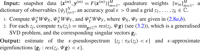
To overcome this issue, algorithm 2 computes practical approximations of  $\epsilon$-pseudospectra with rigorous convergence guarantees. Assuming convergence of the quadrature rule in § 2.2, in the limit $M\rightarrow \infty$, the key quantity
 \begin{equation} \tau_N(\lambda) = \min_{\pmb{g}\in\mathbb{C}^{N}} {res}(\lambda,\varPsi\pmb{g}), \end{equation}
is an upper bound for  $\|(\mathcal {K}-\lambda )^{-1}\|^{-1}$. The output of algorithm 2 is guaranteed to be inside the $\epsilon$-pseudospectrum of $\mathcal {K}$. As $N\rightarrow \infty$ and the grid of points is refined, algorithm 2 converges to the pseudospectrum uniformly on compact subsets of $\mathbb {C}$ (Colbrook & Townsend Reference Colbrook and Townsend2021, theorems B.1 and B.2). In practice the grid $\{z_j\}_{j=1}^k$ is chosen for plotting purposes (e.g. in figure 3). Strictly speaking, we converge to the approximate point pseudospectrum, a more complicated algorithm leads to computation of the full pseudospectrum – see Colbrook & Townsend (Reference Colbrook and Townsend2021, appendix B). For brevity, we have not included a statement of the results. We can then compute the spectrum by taking $\epsilon \downarrow 0$. Algorithm 2 also computes observables $g$ with ${res}(\lambda,g)< \epsilon$, known as $\epsilon$-approximate eigenfunctions. The computational cost of algorithm 2 is ${O}(N^2M+kN^3)$. However, the computation of $\tau _N$ can be done in parallel over the $k$ grid points, and we can refine the grid adaptively near regions of interest.
Algorithm 2 : ResDMD for estimating ε-pseudospectra.
3.3. Choice of dictionary
When  $d$ is large, it can be impractical to store or form the matrix $\mathbb {K}$ since the initial value of $N$ may be huge. In other words, we run into the curse of dimensionality. We consider two common methods to overcome this issue:
(i) DMD: in this case, the dictionary consists of linear functions (see § 2.3.1). It is standard to form a low-rank approximation of
$\sqrt {W}\varPsi _X$ via a truncated SVD as
(3.9)Here,\begin{equation} \sqrt{W}\varPsi_X\approx U_r\varSigma_rV_r^*. \end{equation}$\varSigma _r\in \mathbb {C}^{r\times r}$ is diagonal with strictly positive diagonal entries, and $V_r\in \mathbb {C}^{N\times r}$ and $U_r\in \mathbb {C}^{M\times r}$ have $V_r^*V_r=U_r^*U_r=I_r$. We then form the matrix
(3.10)Note that to fit into our Galerkin framework, this matrix is the transpose of the DMD matrix that is commonly computed in the literature.\begin{equation} \tilde{\mathbb{K}}=(\sqrt{W}\varPsi_XV_r)^{\dagger}\sqrt{W} \varPsi_YV_r=\varSigma_r^{{-}1}U_r^*\sqrt{W}\varPsi_YV_r=V_r^* \mathbb{K}V_r\in\mathbb{C}^{r\times r}. \end{equation}(ii) Kernelised EDMD (kEDMD): kEDMD (Williams et al. Reference Williams, Rowley and Kevrekidis2015b) aims to make EDMD practical for large
$d$. Supposing that $\varPsi _X$ is of full rank, kEDMD constructs a matrix with an identical formula to (3.10) when $r=M$, for which we have the equivalent form
(3.11)Suitable matrices\begin{equation} \tilde{\mathbb{K}}=(\varSigma_M^{\dagger} U_M^*)(\sqrt{W}\varPsi_Y \varPsi_X^*\sqrt{W})(U_M\varSigma_M^{\dagger}). \end{equation}$U_M$ and $\varSigma _M$ can be recovered from the eigenvalue decomposition $\sqrt {W}\varPsi _X\varPsi _X^*\sqrt {W}=U_M\varSigma _M^2U_M^*$. Moreover, both matrices $\sqrt {W}\varPsi _X\varPsi _X^*\sqrt {W}$ and $\sqrt {W}\varPsi _Y\varPsi _X^*\sqrt {W}$ can be computed using inner products. The kEDMD applies the kernel trick to compute the inner products in an implicitly defined reproducing Hilbert space $\mathcal {H}$ with inner product $\langle {\cdot },{\cdot }\rangle _{\mathcal {H}}$ (Scholkopf Reference Scholkopf2001). A positive–definite kernel function $\mathcal {S}:\varOmega \times \varOmega \rightarrow \mathbb {R}$ induces a feature map $\varphi :\mathbb {R}^d\rightarrow \mathcal {H}$ so that $\langle \varphi (\pmb {x}), \varphi (\pmb {y})\rangle _{\mathcal {H}}=\mathcal {S}(\pmb {x},\pmb {y})$. This leads to an implicit choice of (typically nonlinear) dictionary $\varPsi (\pmb {x})$, that is dependent on the kernel function, so that $\varPsi (\pmb {x})\varPsi (\pmb {y})^*=\langle \varphi (\pmb {x}),\varphi (\pmb {y})\rangle _{\mathcal {H}}=\mathcal {S}(\pmb {x},\pmb {y})$. Often $\mathcal {S}$ can be evaluated in ${O}(d)$ operations, meaning that $\tilde {\mathbb {K}}$ is constructed in ${O}(dM^2)$ operations.


In either of these two cases, the approximation of  $\mathcal {K}$ is equivalent to using a new dictionary with feature map $\varPsi (\pmb {x})V_r\in \mathbb {C}^{1\times r}$. In the case of DMD, we found it beneficial to use the mathematically equivalent choice $\varPsi (\pmb {x})V_r\varSigma _r^{-1}$, which is numerically better conditioned. To see why, note that $\sqrt {W}\varPsi _XV_r\varSigma _r^{-1}\approx U_r$ and $U_r$ has orthonormal columns.
3.3.1. The problem of vanishing residual estimates
Suppose that  $\sqrt {W}\varPsi _XV_r$ has full row rank, so that $r=M$, and that $\pmb {v}\in \mathbb {C}^{M}$ is an eigenvector of $\tilde {\mathbb {K}}$ with eigenvalue $\lambda$. This means that $(\sqrt {W}\varPsi _XV_M)^{\dagger} \sqrt {W}\varPsi _YV_M \pmb {v}=\lambda \pmb {v}$. Since $\sqrt {W}\varPsi _XV_M$ has independent rows, $\sqrt {W}\varPsi _XV_M(\sqrt {W}\varPsi _XV_M)^{\dagger} =I_M$ and hence $\sqrt {W}\varPsi _YV_M\pmb {v}=\lambda \sqrt {W}\varPsi _XV_M\pmb {v}$. The corresponding observable is $g(\pmb {x})=\varPsi (\pmb {x})V_M\pmb {v}$ and the numerator of ${res}(\lambda,g)^2$ in (3.2) is equal to $\|\sqrt {W}\varPsi _YV_M\pmb {v}-\lambda \sqrt {W}\varPsi _XV_M\pmb {v}\|^2.$ It follows that ${res}(\lambda,g)=0$. Similarly, if $r$ is too large, ${res}(\lambda,g)$ will be a bad approximation of the true residual.
In other words, the regime  $r\sim M$ prevents the large data convergence $(M\rightarrow \infty )$ of the quadrature rule and (3.4), which holds for a fixed basis and hence a fixed basis size. In turn, this prevents us from being able to apply the results of § 3.2. We next discuss overcoming this issue by using two sets of snapshot data; these could arise from two independent tests of the same system, or by partitioning the measured data into two groups.
3.3.2. Using two subsets of the snapshot data
A simple remedy to avoid the problem in § 3.3.1 is to consider two sets of snapshot data. We consider an initial set  $\{\tilde {\pmb {x}}^{(m)},\tilde {\pmb {y}}^{(m)}\}_{m=1}^{M'}$, that we use to form our dictionary. We then apply ResDMD to the computed dictionary with a second set of snapshot data $\{\hat {\pmb {x}}^{(m)},\hat {\pmb {y}}^{(m)}\}_{m=1}^{M''}$, allowing us to prove convergence as $M''\rightarrow \infty$.
How to acquire a second set of snapshot data depends on the problem and method of data collection. Given snapshot data with random and independent  $\{\pmb {x}^{(m)}\}$, one can split up the snapshot data into two parts. For initial conditions that are distributed according to a high-order quadrature rule, if one already has access to $M'$ snapshots, then one must typically go back to the original dynamical system and request $M''$ further snapshots. For ergodic sampling along a trajectory, we can let $\{\tilde {\pmb {x}}^{(m)},\tilde {\pmb {y}}^{(m)}\}_{m=1}^{M'}$ correspond to the initial $M'+1$ points of the trajectory ( $\tilde {\pmb {x}}^{(m)}=F^{m-1}(\pmb {x}_0)$ for $m=1,\ldots,M'$) and let $\{\hat {\pmb {x}}^{(m)},\hat {\pmb {y}}^{(m)}\}_{m=1}^{M''}$ correspond to the initial $M''+1$ points of the trajectory ( $\hat {\pmb {x}}^{(m)}=F^{m-1}(\pmb {x}_0)$ for $m=1,\ldots,M''$).
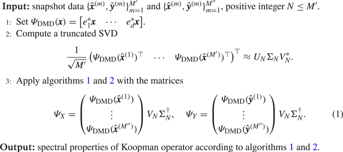
Algorithm 3 : ResDMD with DMD selected observables.
Algorithm 4 : ResDMD with kEDMD selected observables.
In the case of DMD, algorithm 3 summarises the two-stage process. Often a suitable choice of  $N$ can be obtained by studying the decay of the singular values of the data matrix or the condition number of the matrix $\varPsi _X^*W\varPsi _X$. When $M'\leq d$, the computational cost of steps 2 and 3 of algorithm 3 are ${O}(d{M'}^2)$ and ${O}(Nd{M''})$, respectively.
In the case of kEDMD, we follow Colbrook & Townsend (Reference Colbrook and Townsend2021), and algorithm 4 summarises the two-stage process. The choice of kernel  $\mathcal {S}$ determines the dictionary and the best choice depends on the application. In the following experiments, we use the Laplacian kernel $\mathcal {S}(\pmb {x},\pmb {y})=\exp (-\gamma {\|\pmb {x}-\pmb {y}\|})$, where $\gamma$ is the reciprocal of the average $\ell ^2$-norm of the snapshot data after it is shifted to have mean zero.
We can now apply the theory of § 3.2 in the limit  $M''\rightarrow \infty$. It is well known that the eigenvalues computed by DMD and kEDMD may suffer from spectral pollution. However, crucially in our setting, we do not directly use these methods to compute spectral properties of $\mathcal {K}$. Instead, we only use them to select a good dictionary of size $N$, after which our rigorous ResDMD algorithms can be used. Moreover, we use $\{\hat {\pmb {x}}^{(m)},\hat {\pmb {y}}^{(m)}\}_{m=1}^{M''}$ to check the quality of the constructed dictionary. By studying the residuals and using the error control in ResDMD, we can tell a posteriori whether the dictionary is satisfactory and whether $N$ is sufficiently large.
Finally, it is worth pointing out that the above choices of dictionaries are certainly not the only choices. ResDMD can be applied to any suitable choice. For example, one could use other data-driven methods such as diffusion kernels (Giannakis et al. Reference Giannakis, Kolchinskaya, Krasnov and Schumacher2018) or trained neural networks (Li et al. Reference Li, Dietrich, Bollt and Kevrekidis2017; Murata, Fukami & Fukagata Reference Murata, Fukami and Fukagata2020).
4. Spectral measures
Many physical systems described by (1.1) are measure preserving (preserve volume). Examples include Hamiltonian flows (Arnold Reference Arnold1989), geodesic flows on Riemannian manifolds (Dubrovin, Fomenko & Novikov Reference Dubrovin, Fomenko and Novikov1991, Chapter 5), Bernoulli schemes in probability theory (Shields Reference Shields1973) and ergodic systems (Walters Reference Walters2000). The Koopman operator  $\mathcal {K}$ associated with a measure-preserving dynamical system is an isometry, i.e. $\|\mathcal {K}g\|=\|g\|$ for all observables $g\in \mathcal {D}(\mathcal {K})=L^2(\varOmega,\omega )$. In this case, spectral measures provide a way of including continuous spectra in the Koopman mode decomposition. This inclusion is beneficial in the case of turbulent flows where a priori knowledge of the spectra (e.g. whether it contains a continuous part) may be unknown. The methods described in this section allow us to compute continuous spectra.
4.1. Spectral measures and Koopman mode decompositions
Given an observable  $g\in L^2(\varOmega,\omega )$ of interest, the spectral measure of $\mathcal {K}$ with respect to $g$ is a measure $\nu _g$ defined on the periodic interval $[-{\rm \pi},{\rm \pi} ]_{{per}}$. If $g$ is normalised so that $\|g\|=1$, then $\nu _g$ is a probability measure, otherwise $\nu _g$ is a positive measure of total mass $\|g\|^2$. We provide a mathematical description of spectral measures in § A for completeness. The reader should think of these measures as supplying a diagonalisation of $\mathcal {K}$.
For example, the decomposition in (A3) provides important information on the evolution of dynamical systems. Suppose that there is no singular continuous spectrum, then any  $g\in L^2(\varOmega,\omega )$ can be written as
 \begin{equation} g=\sum_{\lambda\in{\sigma}_{{p}}(\mathcal{K})}c_\lambda \varphi_\lambda+\int_{[-{\rm \pi},{\rm \pi}]_{{per}}}\phi_{\theta,g}\, {\rm d} \theta, \end{equation}
where  ${\sigma }_{{p}}(\mathcal {K})$ is the set of eigenvalues of $\mathcal {K}$, the $\varphi _\lambda$ are the eigenfunctions of $\mathcal {K}, c_\lambda$ are expansion coefficients and the density of the absolutely continuous part of $\nu _g$ is $\rho _g(\theta )=\langle \phi _{\theta,g},g\rangle$. One should think of $\phi _{\theta,g}$ as a ‘continuously parametrised’ collection of eigenfunctions. Using (4.1), one obtains the Koopman mode decomposition (Mezić Reference Mezić2005)
 \begin{equation} g(\pmb{x}_n)=[\mathcal{K}^ng](\pmb{x}_0)=\sum_{\lambda \in{\sigma}_{{p}}(\mathcal{K})}c_{\lambda}\lambda^n \varphi_\lambda(\pmb{x}_0)+\int_{[-{\rm \pi},{\rm \pi}]_{{per}}}\, {\rm e}^{{\rm i}n\theta}\phi_{\theta,g}(\pmb{x}_0)\, {\rm d} \theta. \end{equation}
For characterisations of the dynamical system in terms of these decompositions, see Halmos (Reference Halmos2017), Mezić (Reference Mezić2013) and Zaslavsky (Reference Zaslavsky2002). Typically, the eigenvalues correspond to isolated oscillation frequencies in the fluid flow and the growth rates of stable and unstable modes, whilst the continuous spectrum corresponds to chaotic motion. Computing the measures  $\nu _g$ provides us with a diagonalisation of the nonlinear dynamical system in (1.1).
4.2. Spectral measures and autocorrelations
The Fourier coefficients of  $\nu _g$ are given by
 \begin{equation} \widehat{\nu_g}(n):=\frac{1}{2{\rm \pi}}\int_{[-{\rm \pi},{\rm \pi}]_{{per}}} \, {\rm e}^{-{\rm i}n\theta}\,{\rm d} \nu_g(\theta),\quad n\in\mathbb{Z}. \end{equation}
These Fourier coefficients can be expressed in terms of correlations  $\langle \mathcal {K}^n g,g\rangle$ and $\langle g,\mathcal {K}^n g\rangle$ (Colbrook & Townsend Reference Colbrook and Townsend2021). That is, for $g\in L^2(\varOmega,\omega )$
 \begin{equation} \widehat{\nu_g}(n)=\frac{1}{2{\rm \pi}}\langle \mathcal{K}^{{-}n}g,g\rangle, \quad n<0, \quad \widehat{\nu_g}(n)=\frac{1}{2{\rm \pi}}\langle g, \mathcal{K}^ng\rangle,\quad n\geq 0. \end{equation}
From (4.4a,b), we see that  $\widehat {\nu _{g}}(-n)=\overline {\widehat {\nu _{g}}(n)}$ for $n\in \mathbb {Z}$. In particular, $\nu _g$ is completely determined by the forward-time dynamical autocorrelations $\langle g,\mathcal {K}^ng\rangle$ with $n\geq 0$. Equivalently, the spectral measure of $\mathcal {K}$ with respect to $g\in L^2(\varOmega,\omega )$ is a signature for the forward-time dynamics of (1.1). This connection allows us to interpret spectral measures as an infinite-dimensional version of power spectra in § 4.5.
4.3. Computing autocorrelations
To approximate spectral measures, we make use of the relation (4.4a,b) between the Fourier coefficients of  $\nu _g$ and the autocorrelations $\langle g,\mathcal {K}^ng\rangle$. There are typically three ways to compute the autocorrelations, corresponding to the three scenarios discussed in § 2.3:
1. Random sampling: the autocorrelations can be approximated as
(4.5)\begin{equation} \langle g,\mathcal{K}^ng\rangle\approx\frac{1}{M} \sum_{m=1}^{M}g(\pmb{x}^{(m)})\overline{[\mathcal{K}^ng](\pmb{x}^{(m)})}. \end{equation}2. High-order quadrature: the autocorrelations can be approximated as
(4.6)\begin{equation} \langle g,\mathcal{K}^ng\rangle = \int_{\varOmega}g(\pmb{x}) \overline{[\mathcal{K}^ng](\pmb{x})}\,{\rm d} \omega(\pmb{x}) \approx\sum_{m=1}^{M}w_mg(\pmb{x}^{(m)})\overline{[\mathcal{K}^ng] (\pmb{x}^{(m)})}. \end{equation}3. Ergodic sampling: the autocorrelations can be approximated as
(4.7)\begin{equation} \langle g,\mathcal{K}^ng\rangle\approx \frac{1}{M-n} \sum_{m=0}^{M-n-1} g(\pmb{x}_{m})\overline{[\mathcal{K}^ng] (\pmb{x}_{m})}= \frac{1}{M-n} \sum_{m=0}^{M-n-1} g(\pmb{x}_{m})\overline{g(\pmb{x}_{m+n})}. \end{equation}


The first two methods require multiple snapshots of the form  $\{\pmb {x}_0^{(m)},\ldots, \pmb {x}_{n}^{(m)}\}$, with $[\mathcal {K}^ng](\pmb {x}_0^{(m)})=g(\pmb {x}_{n}^{(m)})$. Ergodic sampling only requires a single trajectory, and the ergodic averages in (4.7) can be rewritten as discrete (non-periodic) convolutions. Thus, by zero padding, the fast Fourier transform computes all averages simultaneously and rapidly.
4.4. Computing spectral measures
We suppose now that one has already computed the autocorrelations  $\langle g,\mathcal {K}^ng\rangle$ for $0\leq n\leq N_{{ac}}$. In practice, given a fixed data set of $M$ snapshots, we choose a suitable $N_{{ac}}$ by checking for convergence of the autocorrelations by comparing with smaller values of $M$. Following Colbrook & Townsend (Reference Colbrook and Townsend2021), we define an approximation to $\nu _g$ as
 \begin{equation} \nu_{g,N_{{ac}}}(\theta)=\sum_{n={-}N_{{ac}}}^{N_{{ac}}} \varphi \left(\frac{n}{N_{{ac}}}\right)\widehat{\nu_g}(n)\,{\rm e}^{{\rm i}n\theta}. \end{equation}
The function  $\varphi : [-1,1]\rightarrow \mathbb {R}$ is often called a filter function (Tadmor Reference Tadmor2007; Hesthaven Reference Hesthaven2017) and $\varphi (x)$ is close to $1$ when $x$ is close to $0$, but tapers to $0$ near $x=\pm 1$. Algorithm 5 summarises the approach, and the choice of $\varphi$ affects the convergence.
For  $m\in \mathbb {N}$, suppose that $\varphi$ is even, continuous and compactly supported on $[-1,1]$ with
(a)
$\varphi \in \mathcal {C}^{m-1}([-1,1])$;(b)
$\varphi (0)=1$ and $\varphi ^{(n)}(0)=0$ for any integer $1\leq n\leq m-1$;(c)
$\varphi ^{(n)}(1)=0$ for any integer $0\leq n\leq m-1$,(d)
$\varphi |_{[0,1]}\in \mathcal {C}^{m+1}([0,1])$.


Then, we have the following forms of convergence (Colbrook & Townsend Reference Colbrook and Townsend2021, § 3):
(i) Under suitable (local) smoothness assumptions,
$|\nu _{g,N_{{ac}}}(\theta )-\rho _g(\theta )|= {O}(N_{{ac}}^{-m} \log (N_{{ac}}))$,(ii) A suitable rescaling of
$\nu _{g,N_{{ac}}}\ (\theta_0) $ approximates the point spectrum at $\theta _0$,(iii) For any
$\phi \in \mathcal {C}^{n,\alpha }([-{\rm \pi},{\rm \pi} ]_{{per}})$,
(4.9)
\begin{equation}
\left|\int_{[-{\rm \pi},{\rm \pi}]_{{per}}}
\phi(\theta)\nu_{g,N_{{ac}}} (\theta)\,{\rm d} \theta -
\int_{[-{\rm \pi},{\rm \pi}]_{{per}}} \phi(\theta)\,{\rm d}
\nu_g(\theta)\right| \lesssim
\|\phi\|_{\mathcal{C}^{n,\alpha}} (N_{{ac}}^{-(n+\alpha)}+
N_{{ac}}^{{-}m}\log(N_{{ac}})).
\end{equation}


This last property is known as weak convergence. One should think of  $\nu _{g,N_{{ac}}}$ as a smooth function that approximates the spectral measure $\nu _g$ to order ${O}(N_{{ac}}^{-m}\log (N_{{ac}}))$, with a frequency smoothing scale of ${O}(N_{{ac}}^{-m})$.
Algorithm 5 : Approximating spectral measures from autocorrelations.
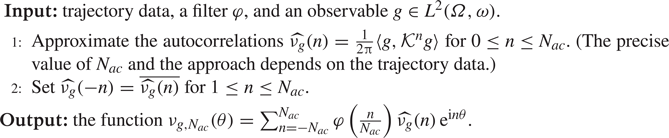
One can also compute spectral measures without autocorrelations. Colbrook & Townsend (Reference Colbrook and Townsend2021) also develop high-order methods based on rational kernels that approximate spectral measures using the ResDMD matrices. Computing suitable residuals allows an adaptive and rigorous selection of the smoothing parameter used in the convolution. In particular, this set-up allows us to deal with general snapshot data  $\{\pmb {x}^{(m)},\pmb {y}^{(m)}=F(\pmb {x}^{(m)})\}_{m=1}^M$ without the need for long trajectories. For brevity, we omit the details.
4.5. Interpretation of Koopman spectral measures as power spectra
We can interpret algorithm 5 as an approximation of the power spectrum of the signal  $g(\pmb {x}(t))$, given by Glegg & Devenport (Reference Glegg and Devenport2017, chapter 8)
 \begin{equation} S_{gg}(f)=\int_{{-}T}^TR_{gg}(t)\, {\rm e}^{2{\rm \pi} {\rm i} ft}\, {\rm d} t, \end{equation}
over a time window  $[-T,T]$ and for frequency $f$ (measured in Hertz). Here, $R_{gg}(t)$ is the delay autocorrelation function, defined for $t\geq 0$ as
 \begin{equation} R_{gg}(t)=\langle g,g\circ F_t\rangle, \end{equation}
where  $F_t$ is the forward-time propagator for a time step $t$. In particular, we have
 \begin{equation} R_{gg}(n{\rm \Delta}
t)=\left\{\begin{array}{@{}ll} \langle g,\mathcal{K}^ng\rangle
& \text{if }n\geq 0\\ \overline{\langle
g,\mathcal{K}^{{-}n}g\rangle}= \langle\mathcal{K}^{{-}n}
g,g\rangle & \text{otherwise} \end{array}\right. .
\end{equation}
\begin{equation} R_{gg}(n{\rm \Delta}
t)=\left\{\begin{array}{@{}ll} \langle g,\mathcal{K}^ng\rangle
& \text{if }n\geq 0\\ \overline{\langle
g,\mathcal{K}^{{-}n}g\rangle}= \langle\mathcal{K}^{{-}n}
g,g\rangle & \text{otherwise} \end{array}\right. .
\end{equation}
We apply windowing and multiply the integrand in (4.10) by the filter function  $\varphi (t/T)$. We then discretise the resulting integral using the trapezoidal rule (noting that the endpoint contributions vanish) with step size ${\rm \Delta} t=T/N_{{ac}}$ to obtain the approximation
 \begin{align} \frac{{S}_{gg}(f)}{2{\rm \pi}{\rm \Delta} t}\approx\sum_{n={-}N_{{ac}}}^{N_{{ac}}} \varphi\left(\frac{n}{N_{{ac}}}\right)\frac{R_{gg}(n{\rm \Delta} t)}{2{\rm \pi}} \, {\rm e}^{{\rm i}n(2{\rm \pi} f{\rm \Delta} t)}=\sum_{n={-}N_{{ac}}}^{N_{{ac}}} \varphi\left(\frac{n}{N_{{ac}}}\right)\widehat{\nu_g}(n)\, {\rm e}^{{\rm i}n(2{\rm \pi} f{\rm \Delta} t)}. \end{align}
It follows that  $\nu _{g,N_{{ac}}}(2{\rm \pi} f{\rm \Delta} t)$ can be understood as a discretised version of ${S}_{gg}(f)/(2{\rm \pi} {\rm \Delta} t)$ over the time window $[-T,T]$. Taking the limit $N_{{ac}}\rightarrow \infty$ with $(2{\rm \pi} {\rm \Delta} t) f=\theta$, we see that $\nu _g$ is an appropriate limit of the power spectrum with time resolution ${\rm \Delta} t$. There are two key benefits of using $\nu _g$. First, we do not explicitly periodically extend the signal to compute autocorrelations and thus avoid the problem of broadening. Instead, we window in the frequency domain. Second, we have rigorous convergence theory as $N_{{ac}}\rightarrow \infty$. We compare spectral measures with power spectra in § 6.
5. Example I: flow past a cylinder wake
We first verify our method by considering the classic example of low Reynolds number flow past a circular cylinder, as focused on by Bagheri (Reference Bagheri2013). Due to its simplicity and its relevance in engineering, this is one of the most studied examples in modal-analysis techniques (Rowley & Dawson Reference Rowley and Dawson2017, table 3), (Chen et al. Reference Chen, Tu and Rowley2012; Taira et al. Reference Taira, Hemati, Brunton, Sun, Duraisamy, Bagheri, Dawson and Yeh2020). We consider the post-transient regime with  $Re=100$, corresponding to periodic oscillations on a stable limit cycle. The Koopman operator of the flow has a pure point spectrum with a lattice structure on the unit circle (Bagheri Reference Bagheri2013) (this is not to be confused with the two-dimensional lattice for the regime on and near the limit cycle that includes transient modes inside the unit disc).
5.1. Computational set-up
The flow around a circular cylinder of diameter  $D$ is obtained using an incompressible, two-dimensional lattice-Boltzmann computational fluid dynamics (CFD) flow solver. The solver uses the two-dimensional 9-velocity lattice model (commonly referred to as D2Q9) lattice and BGKW (Bhatnagar, Gross & Krook Reference Bhatnagar, Gross and Krook1954) collision models to calculate the velocity field. The temporal resolution (time step) of the flow simulations is such that the Courant–Friedrichs–Lewy number is unity on the uniform numerical grid. However, this results in a very finely resolved flow field and hence a large volume of data. An initial down-sampling study revealed that storing 12 snapshots of flow field data within a period of vortex shedding still enables us to use our analysis tools without affecting the results. We also verified our results against higher grid resolution for the CFD solver. The computational domain size is $18D$ in length and $5D$ in height. The cylinder is positioned $2D$ downstream of the inlet at the mid-height of the domain. The cylinder walls and the side walls are defined as bounce-back no-slip walls, and a parabolic velocity inlet profile is defined at the inlet of the domain such that $Re=100$. The outlet is defined as a non-reflecting outflow. For a detailed description of the solver, we refer the reader to Józsa et al. (Reference Józsa, Szőke, Teschner, Könözsy and Moulitsas2016) and Szőke et al. (Reference Szőke, Jozsa, Koleszár, Moulitsas and Könözsy2017).
5.2. Results
We collect snapshot data of the velocity field along a single trajectory in the post-transient regime of the flow and split the data into two data sets according to § 3.3.2. The first set  $\{\tilde {\pmb {x}}^{(m)},\tilde {\pmb {y}}^{(m)}\}_{m=1}^{M'}$ corresponds to $M'=500$ snapshots. We then collect $M''=1000$ further snapshots $\{\hat {\pmb {x}}^{(m)},\hat {\pmb {y}}^{(m)}\}_{m=1}^{M''}$, where $\hat {\pmb {x}}^{(1)}$ corresponds to approximately 40 time periods of vortex shedding later than $\tilde {\pmb {x}}^{(M')}$. We use algorithms 3 and 4, which we refer to as a linear dictionary (obtained using DMD) and a nonlinear dictionary (obtained using kEDMD), respectively. For both dictionaries, we use $N=200$ functions. Similar results and conclusions are obtained when varying $N,M'$ and $M''$.
Figure 3 shows values of  $\tau _N$ (pseudospectral contours) computed using algorithm 2, where $\tau _N$ is the minimal residual in (3.8). The circular contours show excellent agreement with the distance to the spectrum, which is the unit circle in this example. The spectrum corresponds to the closure of the set of eigenvalues which wrap around the circle. The eigenvalues of the finite $N\times N$ Galerkin matrix $\mathbb {K}$ in each case are shown as red dots. The linear dictionary demonstrates spectral pollution, i.e. ‘spurious modes’, all of which are easily detected by ResDMD (e.g. algorithm 1). Generically, spectral pollution can occur anywhere inside the essential numerical range of $\mathcal {K}$ (Pokrzywa Reference Pokrzywa1979), which in this case is the complex unit disc. Whether spectral pollution occurs is a subtle issue that is highly dependent on the dictionary. In our case, we observed a reduction in spectral pollution for smaller $N$, with pollution occurring once the linear dictionary cannot approximate the higher-order modes. Detecting when this occurs is a considerable challenge; hence, methods such as algorithm 2 are needed, particularly when we do not know the spectrum a priori.
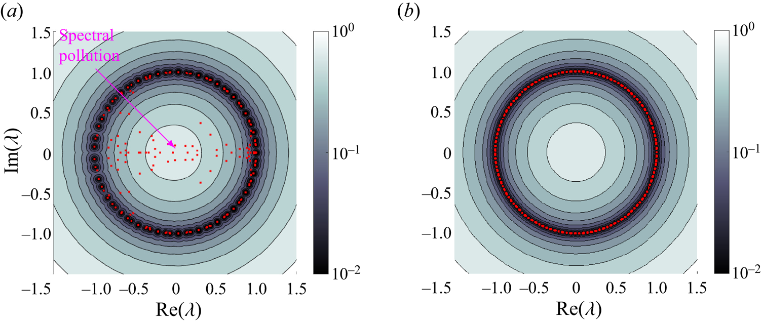
Figure 3. Pseudospectral contours computed using algorithm 2 for the cylinder wake example, using a linear dictionary (a) and a nonlinear dictionary (b). The eigenvalues of the finite Galerkin matrices  $\mathbb {K}$ are shown as red dots in both cases. The computed residuals allow ResDMD to detect spectral pollution (spurious modes); (a) $\tau _{200}(\lambda )$, linear dictionary and (b) $\tau _{200}(\lambda )$, nonlinear dictionary.
Figure 4 shows the convergence of  $\tau _N(-0.5)$ (see (3.8)) as we vary $N$ and $M''$. As expected, we see convergence as $M''\rightarrow \infty$. Moreover, $\tau _N(-0.5)$ decreases and converges monotonically down to $\|(\mathcal {K}+0.5)^{-1}\|^{-1}=0.5$ as $N$ increases. Although both choices of dictionary behave similarly in figure 4, this is not the case for other choices of $\lambda$, as is evident near $\lambda =-1$ in figure 3.

Figure 4. Convergence of  $\tau _N(-0.5)$ as $M''$ (the number of snapshots used to build the ResDMD matrices) increases. The plots show the clear monotonicity of $\tau _N(-0.5)$, which decreases to $\|(\mathcal {K}+0.5)^{-1}\|^{-1}=0.5$ as $N$ increases. (a) linear dictionary; (b) nonlinear dictionary.
Figure 5 shows the eigenvalues of the finite  $N\times N$ Galerkin $\mathbb {K}$ as a phase-residual plot. Some eigenvalues computed using the linear dictionary have minimal relative residuals of approximately $10^{-8}$. Since we compute the squared relative residual in (3.2) and then take a square root, and due to the floating point arithmetic used in the software, these small residuals are effectively the level of $\sqrt {\epsilon _{{mach}}}$. The linear dictionary also has severe spectral pollution. In contrast, the nonlinear dictionary captures the lattice structure of the eigenvalues much better. We have labelled the different branches of the phase as the eigenvalues (powers of the fundamental eigenvalues) wrap around the unit circle.

Figure 5. Phase-residual plot of the eigenvalues of  $\mathbb {K}$. The linear dictionary has very small residuals for the lower modes, yet also suffers from severe spectral pollution. The nonlinear dictionary demonstrates the lattice structure of the Koopman eigenvalues. Branches of the phase as the eigenvalues wrap around the unit circle are labelled. (a) ${res} (\lambda _j, g_{(j)})$, linear dictionary and (b) ${res} (\lambda _j, g_{(j)})$, nonlinear dictionary.
To investigate these points further, figure 6 plots the errors of the eigenvalues, the relative residuals, and the errors of the associated eigenspaces. For each case of dictionary, we first compute a reference eigenvalue  $\lambda _1\approx 0.9676 + 0.2525i$ corresponding to the first mode, and the corresponding eigenfunction $g_{(1)}$. For each $j$, we compare the computed eigenvalue $\lambda _j$ with $\lambda _1^j$. The computed residual satisfies ${res}(\lambda _j,g_{(j)})\geq \tau _{200}(\lambda _j)\geq |\lambda _j-\lambda _1^j|$, confirming that algorithm 1 provides error bounds on the computed spectra. We evaluate $g_{(1)}^j$ and $g_{(j)}$ at the points $\{\hat {\pmb {x}}^{(m)}\}_{m=1}^{M''}$, and the ‘eigenspace error’ corresponds to the subspace angle between the linear spans of the resulting vectors (Colbrook & Hansen Reference Colbrook and Hansen2019, (1.4)). The linear dictionary does an excellent job at capturing the lower spectral content, up to about $j=35$, but is unable to capture the high-order eigenfunctions that are strongly nonlinear (as functions on the state space). In contrast, the nonlinear dictionary does a much better job capturing the higher-order spectral information. For this problem, only a few Koopman modes are needed to reconstruct the flow. However, for some problems, having nonlinear functions in the dictionary is essential to capture the dynamics (e.g. see Brunton et al. (Reference Brunton, Brunton, Proctor and Kutz2016), and our examples in §§ 7 and 8). One is completely free to choose the dictionary used in ResDMD. For example, one could also use a mixture of the DMD and kEDMD computed dictionaries, or other methods. For example, figure 6(c) shows that taking a union of the two dictionaries can capture the low order modes with high accuracy and also cope with the nonlinearities of the high order modes.

Figure 6. Errors of the computed spectral information of each mode. (a) linear dictionary; (b) nonlinear dictionary; (c) union of dictionaries.
Figures 7 and 8 show examples of Koopman modes (see (2.15)) for the  $x$ component of the velocity, computed using the linear and nonlinear dictionaries, respectively. Each Koopman eigenfunction is normalised so that the vector $\sqrt {W}\varPsi _XV(:,j)$ has norm $1$. Modes $1$ and $2$ show excellent agreement between the two dictionary choices and can also be compared with Taira et al. (Reference Taira, Hemati, Brunton, Sun, Duraisamy, Bagheri, Dawson and Yeh2020, figure 3). However, for the higher mode (mode 20), the two results bear little similarity. Mode 20 may be seen as a turbulence–turbulence interaction mode that potentially stems from the nonlinear convection term of the Navier–Stokes equation. From a mathematical aspect, the difference in the 20th Koopman mode is because one cannot accurately capture highly nonlinear behaviour with a linear approximation; eventually, there must be a breakdown in the approximation. Whilst the low-order linear approximation does capture the (weakly) nonlinear low-order behaviour, at higher order, the nonlinearity is strengthened. Thus the attempt to capture it linearly is poor. Recall that the Koopman modes correspond to the vector-valued expansion coefficients of the state in the approximate eigenfunctions, as opposed to the eigenfunctions themselves. Thus, the difference indicates that for high-order modes, nonlinearity becomes important in this expansion. We can be assured by the residual measure in the ResDMD algorithm that the modes arising from using the nonlinear dictionary are physical features of the flow and not spurious. ResDMD, therefore, brings certainty to the high-order modal analysis of this classic example, which can be lacking in prior DMD or EDMD approaches.

Figure 7. Koopman modes for the cylinder wake, computed using the linear dictionary.

Figure 8. Koopman modes for the cylinder wake, computed using the nonlinear dictionary (see graphical abstract).
6. Example II: embedded shear layer in a turbulent boundary layer flow
We now use our method to analyse a high Reynolds number turbulent flow with a fine temporal resolution. We consider the turbulence structure within a turbulent boundary layer over a flat plate both with and without an embedded shear profile. A shear profile is achieved by permitting a steady flow to be injected through a section of the plate. Turbulent boundary layer flow can be considered a challenging test case for DMD algorithms, particularly when assessing potential nonlinear flow behaviours, and the wide range of length scales present in a high Reynolds number flow problem. On the other hand, the embedded shear layer is anticipated to have a set of characteristic length scales with a broadband energy distribution.
6.1. Experimental set-up
We consider two cases of turbulent boundary layer flow, a canonical (baseline) and one with an embedded shear layer. Both cases are generated experimentally and detailed in Szőke, Fiscaletti & Azarpeyvand (Reference Szőke, Fiscaletti and Azarpeyvand2020). For clarity, we briefly recall the key features and illustrate the experimental set-up in figure 9. The baseline case consists of a canonical, zero-pressure-gradient turbulent boundary layer (TBL) passing over a flat plate (no flow control turned on). The friction Reynolds number is  $Re_\tau = 1400$. In the experiments, the development of a shear layer is triggered using perpendicular flow injection (active flow control) through a finely perforated sheet, denoted by $u_{AFC}$. The velocity field is sensed at several positions downstream of the flow control area by traversing a hot-wire probe across the entire boundary layer. The data gathered using the hot-wire sensor provides a fine temporal description of the flow. For a more detailed description of the experimental set-up and the flow field, see Szőke et al. (Reference Szőke, Fiscaletti and Azarpeyvand2020). A wide range of downstream positions and flow control severity values were considered in the original study to assess flow control's effects on trailing edge noise. Here, the same data are used, but we focus our attention on one streamwise position (labelled as BL3 in figure 9) and consider a flow injection case where a shear layer develops as a result of perpendicular flow injection. Similar qualitative comparisons (against power spectral densities) were found for different sensor locations and different injection angles.

Figure 9. Schematic of the experimental set-up for a boundary layer with embedded shear profile, and side view of the boundary layer near the flow control region.
6.2. Results
The fine temporal resolution of the flow field enables us to assess the spectral properties of the flow. We use algorithm 5 to calculate the spectral measures of the flow and compare our results with the power spectral density (PSD) obtained using Welch's PSD estimate as described in Szőke et al. (Reference Szőke, Fiscaletti and Azarpeyvand2020). For this example, DMD-type methods cannot robustly approximate the Koopman operator of the underlying dynamical system since data are only collected along a single line. However, algorithm 5 can still be used to compute the spectral measures of the Koopman operator.
As a first numerical test, we compute spectral measures of the data collected at 10 % of the undisturbed boundary layer height ( $y/\delta _0 = 0.1$). We then integrate this spectral measure against the test function $\phi (\theta )=\exp (\sin (\theta ))$. Rather than being a physical example, this is chosen to demonstrate the convergence of our method. We consider the integral computed using the PSD (4.10) with a window size of $N_{{ac}}$ for direct comparison, and algorithm 5 for choices of filter $\varphi _{hat}(x) = 1-|x|, \varphi _{{\cos }}(x) =\frac {1}{2}(1-\cos ({\rm \pi} x)), \varphi _{{four}}(x))$ $= 1- x^4(-20|x|^3 + 70x^2 - 84|x| + 35)$ and $\varphi _{{bump}}(x)=\exp (-({2}/({1-|x|}))\exp (-{c}/{x^4}))$ ( $c\approx 0.109550455106347$). These filters are first, second, fourth and infinite order, respectively. Figure 10 shows the results, where we see the expected rates of convergence of algorithm 5. In contrast, the PSD approximation initially appears to converge at a second-order rate and then stagnates.

Figure 10. Relative error in integration against the test function  $\phi (\theta )=\exp (\sin (\theta ))$ for data collected at $y/\delta _0=0.1$. Algorithm 5 converges at the expected rates for various filter functions. In contrast, the PSD approximation appears to converge at a second-order rate initially but then stagnates. (a) relative error (injection); (b) relative error (baseline).
Figure 11 compares the spectral measure, as found using algorithm 5, with the PSD (4.10) obtained from direct processing of the experimental data, where we have used a window size of  $N_{{ac}}$ for direct comparison. To directly compare with PSD, we use algorithm 5 with the second-order filter $\varphi _{{\cos }}$. A range of different vertical locations $y/\delta _0$ are considered, where $\delta _0$ is the boundary layer thickness of the baseline case (i.e. $u_{AFC} = 0\ {\rm m}\ {\rm s}^{-1}$). Whilst the high-frequency behaviour is almost identical between the two methods, at low frequencies ( ${<}10$ Hz) the spectral measure returns values approximately ${\sim }1$ dB greater than the PSD processing because the conventional PSD calculation results observe broadening at low frequencies. Figure 12 confirms this and shows the low-frequency values for $N_{{ac}}=4000$ and various choices of filter function. In general, higher-order filters lead to a sharper peak at low frequencies. This comparison also holds for different sensor locations (in figure 9) and different injection angles. As we are assured that the spectral measure rigorously converges, this new method provides the more accurate measure of the power at low frequencies as $N_\mathrm {ac}\rightarrow \infty$.

Figure 11. Comparison of the traditional PSD definition (4.10) with spectral measure (4.13) (referenced to 1 m $^2$ s $^{-2}$), for baseline and injection flows, at a range of vertical heights within the boundary layer. (a) PSD (injection); (b) spectral measure (injection); (c) PSD (baseline); (d) spectral measure (baseline).

Figure 12. Zoomed in values for low frequencies computed using  $N_{{ac}}=4000$ and various choices of filter function. In general, higher order filters lead to a sharper peak at low frequencies. (a) injection; (b) baseline.
7. Example III: wall-jet boundary layer flow
As a further example of TBL flow, we now consider a wall-jet boundary layer (George et al. Reference George, Abrahamsson, Eriksson, Karlsson, Löfdahl and Wosnik2000; Gersten Reference Gersten2015; Kleinfelter et al. Reference Kleinfelter, Repasky, Hari, Letica, Vishwanathan, Organski, Schwaner, Alexander and Devenport2019). Whilst hot-wire probes enable a very fine temporal resolution of the flow field, they are usually restricted to a single point or line in space, and thus preclude the use of many DMD-type methods. On the other hand, time-resolved (TR) PIV offers both spatial and temporal descriptions of the flow. For this example, we assess the performance of the ResDMD algorithm on a set of TR-PIV data. We consider the boundary layer generated by a thin jet ( $h_{jet}=12.7$ mm) injecting air onto a smooth flat wall. As in example II, this case is challenging for regular DMD approaches due to multiple turbulent scales expected within the boundary layer. This section demonstrates the use of ResDMD for a high Reynolds number, turbulent, complicated flow field.
7.1. Experimental set-up
Experiments using TR-PIV are performed at the Wall Jet Wind Tunnel of Virginia Tech as schematically shown in figure 13. For a detailed description of the facility, we refer to Kleinfelter et al. (Reference Kleinfelter, Repasky, Hari, Letica, Vishwanathan, Organski, Schwaner, Alexander and Devenport2019). A two-dimensional two-component TR-PIV system is used to capture the wall-jet flow, and the streamwise origin of the field-of-view (FOV) is  $\hat {x} = 1282.7$ mm downstream of the wall-jet nozzle. We use a jet velocity of $U_j=50$ m s $^{-1}$, corresponding to a jet Reynolds number of $Re_{jet} = h_{jet} U_j /\nu = 63.5 \times 10^3$. The length and height of the FOV are approximately $75 {\rm mm} \times 40\ {\rm mm}$, and the spatial resolution of the velocity vector field is 0.24 mm. This resolution corresponds to dimension $d = 102,300$ in (1.1). The high-speed cameras are operated in a double frame mode, with a rate of 12 000 frame pairs per second, resulting in a fine temporal resolution of 0.083 ms. For a more detailed description of the experimental set-up and flow field, see Kleinfelter et al. (Reference Kleinfelter, Repasky, Hari, Letica, Vishwanathan, Organski, Schwaner, Alexander and Devenport2019) and Szőke et al. (Reference Szőke, Nurani Hari, Devenport, Glegg and Teschner2021).

Figure 13. The schematic of the TR-PIV experiments conducted in the Wall Jet Wind Tunnel of Virginia Tech.
The associated flow has some special properties. It is self-similar, and its main characteristics (boundary layer thickness, edge velocity, skin friction coefficient, etc.) can be accurately calculated a priori through power-law curve fits (Kleinfelter et al. Reference Kleinfelter, Repasky, Hari, Letica, Vishwanathan, Organski, Schwaner, Alexander and Devenport2019). The flow consists of two main regions. Within the region bounded by the wall and the peak in the velocity profile, the flow exhibits the properties of a zero-pressure-gradient TBL. Above this fluid portion, the flow is dominated by a two-dimensional shear layer consisting of rather large, energetic flow structures. While the peak in the velocity profile is  $y_m \approx 18$ mm from the wall in our case, the overall thickness of the wall-jet flow is of the order of 200 mm. The PIV experiments must compromise between a good spatial resolution and capturing the entire flow field. In our case, the FOV was not tall enough to capture the entire wall-jet flow field. For this reason, the standard DMD algorithm under-predicts the energies corresponding to the shear-layer portion of the wall-jet flow as the corresponding length scales fall outside of the limits of the FOV. We also verified our results, in particular the presence of the modes in figure 16, by comparing with different spatial and temporal resolutions.
7.2. Results
We collect snapshot data of the velocity field from two separate realisations of the experiment. We use the first experiment to generate data  $\{\tilde {\pmb {x}}^{(m)},\tilde {\pmb {y}}^{(m)}\}_{m=1}^{M'}$ with $M'=2000$, corresponding to 121 boundary layer turnover times. This data is used to select our dictionary of functions. We then use the second experiment to generate data $\{\hat {\pmb {x}}^{(m)},\hat {\pmb {y}}^{(m)}\}_{m=1}^{M''}$ with $M''=12\ 000$ (a single trajectory of one second of physical flow time and 728 boundary layer turnover times), which we use to generate the ResDMD matrices, as outlined in § 3.3.2.
To demonstrate the need for nonlinear functions in our dictionary, we compute the Koopman mode decomposition of the total kinetic energy of the domain using (2.14). Using this decomposition, we compute forecasts of the total energy from a given initial condition of the system. Figure 14 shows the results, where we average over the  $12\ 000$ initial conditions in the data set and normalise by the true time-averaged kinetic energy. We use algorithm 3 and 4 with $N=2000$, which we refer to as a linear dictionary and nonlinear dictionary, respectively. The importance of including nonlinear functions in the dictionary is clear, and corresponds to a much better approximation of the spectral content of $\mathcal {K}$ near $0$. This is confirmed in figure 15, where we show the eigenpairs and residuals for each choice of dictionary. The eigenvalues of non-normal matrices can be severely unstable to perturbations, particularly for large $N$, so we checked the computation of the eigenvalues of $\mathbb {K}$ by comparing with extended precision and predict a bound of approximately $10^{-10}$ on the numerical error in figure 15. The nonlinear dictionary has smaller residuals and a more resolved spectrum near $1$ with less spectral pollution. Unlike the example in § 5, the boundary of the spectra are not circular. Instead, they appear to be centred around a curve of the form $r=\exp (-c|\theta |)$ (shown as a black curve in the plot), corresponding to successive powers of transient modes. Therefore, we only use the nonlinear dictionary for the rest of this section.

Figure 14. Forecast of total kinetic energy (normalised by the time average of the kinetic energy), averaged over the 12 000 initial conditions. Values closer to  $1$ correspond to better predictions.

Figure 15. The eigenvalues of finite Galerkin matrix  $\mathbb {K}$ for the wall-jet example. For each eigenvalue–eigenvector pair $(\lambda _j,g_{(j)})$, the residual ${res}(\lambda _j,g_{(j)})$ is shown on a colour scale. When truncating the Koopman mode decomposition for figure 16, we kept those modes with residual at most $0.5$. The black curve corresponds to a fit $r=\exp (-c|\theta |)$ of the boundary of the eigenvalues and represents successive powers of modes. (a) ${res} (\lambda _j, g_{(j)})$, linear dictionary and (b) ${res} (\lambda _j, g_{(j)})$, nonlinear dictionary.
To investigate the Koopman modes, we compute the ResDMD Koopman mode decomposition corresponding to (3.6) with an error tolerance of  $\epsilon =0.5$ to get rid of the most severe spectral pollution. The total number of modes used is 656. Figure 16 illustrates a range of Koopman modes that are long-lasting (left-hand column) and transient (right-hand column). Within each figure, the arrows dictate the unsteady fluid structure (computed from the Koopman modes of the velocity fields), with the magnitude of the arrow indicating the local flow speed, and the colour bar denotes the Koopman mode of the velocity magnitude. The corresponding approximate eigenvalues, $\lambda$, and residual bound, $\tau _N$, are provided for each mode. Due to residuals, we can accurately select physical transient modes. We also remark that many of these modes were not detected when using a linear dictionary.

Figure 16. (a,c,e,g) A range of long-lasting modes from the ResDMD Koopman mode decomposition. (b,d, f,h) A range of transient modes from the ResDMD Koopman mode decomposition. The arrows dictate the unsteady fluid structure (computed from the Koopman modes of the velocity fields), with the magnitude of the arrow indicating the local flow speed, and the colour bar denotes the Koopman mode of the velocity magnitude; (a)  $\lambda = 1.0000 +0.0000i$, $\tau _{2000} (\lambda ) = 0.0024$, (b) $\lambda = 0.9837 +0.0057i$, $\tau _{2000} (\lambda ) = 0.0175$, (c) $\lambda = 0.9760 +0.1132i$, $\tau _{2000} (\lambda ) = 0.0539$, (d) $\lambda = 0.9528 +0.0000i$, $\tau _{2000} (\lambda ) = 0.0472$, (e) $\lambda = 0.9700 +0.1432i$, $\tau _{2000} (\lambda ) = 0.0602$, ( f) $\lambda = 0.8948 +0.1065i$, $\tau _{2000} (\lambda ) = 0.1105$, (g) $\lambda = 0.9439 +0.2458i$, $\tau _{2000} (\lambda ) = 0.0765$ and (h) $\lambda = 0.9888 +0.0091i$, $\tau _{2000} (\lambda ) = 0.0146$.
The modes in the left column of figure 16 illustrate the range of rolling eddies within the boundary layer, with the smaller structures containing less energy than the largest structures. Interestingly, the third mode in the left column resembles the shape of ejection-like motions within the boundary layer flow ( $y/y_m<1$). At the same time, larger-scale structures above the boundary layer ( $y/y_m>1$) are also visible. This may be interpreted as a nonlinear interaction in the turbulent flow field that is efficiently captured using the ResDMD algorithm. The transient modes in the right column of figure 16 show a richer structure. We interpret these modes as transient, short-lived turbulence behaviour based on our analysis. Again, the use of the conventional (linear) DMD method does not enable the capture of these modes. The uppermost panel may be seen as the shear layer travelling over the boundary layer ( $y/y_m>1$), with the following panel potentially seen as the breakdown of this transient structure into smaller structures. The third panel may be seen as an interaction between an ejection-type vortex and the shear layer; note the ejection-like shape of negative contours below $y/y_m=1.5$ with a height-invariant positive island of contour at $y/y_m\approx 1.75$. Finally, the bottom-most panel could be seen as a flow uplift out of the boundary layer and further turbulent streaks with counter-rotating properties.
Using the autocorrelation functions of both streamwise ( $u$) and wall-normal ( $v$) velocity components and algorithm 5, we obtain the streamwise wavenumber spectra of the velocity fluctuations, shown in the top row of figure 17. The streamwise-averaged spectral measure of the ergodic component of the flow for both streamwise and vertical unsteady velocities are shown in the bottom row of figure 17. When observing either the wavenumber spectra or the spectral measures of the streamwise velocity component, we see consistent spectra across the different boundary layer heights due to the dominance of the strong shear layer in the wall-jet flow. For the vertical velocity spectra, as one might expect, more energy is observed for both wavenumber spectra and spectral measures with increasing $y/y_m$.

Figure 17. Pre-multiplied streamwise wavenumber spectra (a,b) and spectral measures (c,d) for streamwise ( $u$) and wall-normal ( $v$) velocity components; (a) $k_x |\phi {uu}|$, (b) $k_x |\phi {vv}|$, (c) spectral measure ( $u$ field) and (d) spectral measure ( $v$ field).

Figure 18. Schematic diagram of the laser beam set-up used to generate the laser-induced plasma.
8. Example IV: acoustic signature of laser-induced plasma
So far, our examples of ResDMD have focused on fluid flows. However, the capability of ResDMD to capture nonlinear mechanics can be applied more broadly. Moreover, the computation of residuals allows an efficient compression of the Koopman mode decomposition through (3.6). As our final example, we demonstrate the use of ResDMD on an acoustic example where the sound source of interest exhibits highly nonlinear properties.
8.1. Experimental set-up
We investigate a near-ideal acoustic monopole source that is generated using the laser-optical set-up illustrated in figure 18. When a high-energy laser beam is focused on a point, the air ionises and plasma is generated due to the extremely high electromagnetic energy density (of the order of  $10^{12}$ W m $^{-2}$). As a result of the sudden deposit of energy, the air volume undergoes a sudden expansion that generates a shockwave. The initial propagation characteristics can be modelled using von Neumann's point strong explosion theory (Von Neumann Reference Von Neumann1963), which was originally developed for nuclear explosion modelling. For our ResDMD analysis, we use laser-induced plasma (LIP) sound signature data measured using a 1/8 inch, Bruel & Kjaer (B&K) type 4138 microphone operated using a B&K Nexus module Szőke et al. (Reference Szőke, Devenport, Borgoltz, Alexander, Hari, Glegg, Li, Vallabh and Seyam2022). The data from the microphone are acquired using an NI-6358 module at a sampling rate of $f_s=1.25$ MS s $^{-1}$ (million samples per second). With this apparatus, we can resolve the high-frequency nature of the LIP up to 100 kHz. For a detailed description of the laser-optical set-up, experimental apparatus, and data processing procedures, see Szőke et al. (Reference Szőke, Devenport, Borgoltz, Alexander, Hari, Glegg, Li, Vallabh and Seyam2022) and Szőke & Devenport (Reference Szőke and Devenport2021).
The important acoustic characteristic of the LIP is a short time period of initial supersonic propagation speed, shown as Schlieren images taken over a  $15\ \mathrm {\mu }$s window in figure 19. When observed from the far field, this initial supersonic propagation is observed as a nonlinear characteristic even though the wave speed is supersonic only until approximately 3–4 mm from the optical focal point. During the experiments, 65 realisations of LIP are captured using microphones. Each realisation of LIP is then gated in time such that only the direct propagation path of the LIP remains in the signal (Szőke & Devenport Reference Szőke and Devenport2021). We use this gated data for our ResDMD analysis.

Figure 19. Schlieren images of the initial LIP illustrating the shock wave formation and propagation; (a)  $t=5\ \mathrm {\mu }{\rm s}$, (b) $t=10\ \mathrm {\mu }{\rm s}$, (c) $t=15\ \mathrm {\mu }{\rm s}$ and (d) $t=20\ \mathrm {\mu }{\rm s}$.
8.2. Results
For a positive integer  $d$, we take the state at time step $n$ to be
 \begin{equation} \pmb{x}_n=(p(n) \quad p(n-1)\quad \cdots \quad p(n-d+1))^\top\in\mathbb{R}^d, \end{equation}
where  $p$ is the acoustic pressure. This choice of state corresponds to time-delay embedding, a popular method for DMD-type algorithms (Arbabi & Mezic Reference Arbabi and Mezic2017a; Kamb et al. Reference Kamb, Kaiser, Brunton and Kutz2020; Pan & Duraisamy Reference Pan and Duraisamy2020). When we make future state predictions using the Koopman mode decomposition, there is an additional interpretation of $d$. The value of $d$ corresponds to the initial time interval we use to make future state predictions. This interval is shown as vertical dashed lines in the plots below.
We split the data into three parts. The first 10 realisations of LIP correspond to  $\{\tilde {\pmb {x}}^{(m)},\tilde {\pmb {y}}^{(m)}\}_{m=1}^{M'}$ and are used to train the dictionary. The next 50 realisations correspond to $\{\hat {\pmb {x}}^{(m)},\hat {\pmb {y}}^{(m)}\}_{m=1}^{M''}$, and are used to construct the ResDMD matrices. The final five realisations are used to test the resulting Koopman mode decomposition. We verified our results by comparing different splittings of the data into sets for dictionary learning, matrix construction and testing. We consider two choices of the dictionary. The first is a linear dictionary computed using algorithm 3. The second is the union of the linear dictionary and the dictionary computed using algorithm 4 with $N=200$. We refer to this combined dictionary as the nonlinear dictionary.
Figure 20(a) shows the results of the Koopman mode decomposition (2.15), applied to the first realisation of the experiment in the test set, with  $d=10$. Namely, we approximate the state as
 \begin{align} \pmb{x}_n&\approx \varPsi(\pmb{x}_0)\mathbb{K}^nV [V^{{-}1}(\sqrt{W}\varPsi_X)^{\dagger} \sqrt{W} [\hat{\pmb{x}}^{(1)} \quad \cdots \quad \hat{\pmb{x}}^{(M'')}]^\top]\nonumber\\ &=\varPsi(\pmb{x}_0)V\varLambda^n [V^{{-}1}(\sqrt{W}\varPsi_X)^{\dagger} \sqrt{W}[\hat{\pmb{x}}^{(1)}\quad \cdots\quad \hat{\pmb{x}}^{(M'')}]^\top]. \end{align}
In particular, we test the Koopman mode decomposition on unseen data corresponding to the test set. The values of  $p$ to the left of the vertical dashed line correspond to $\pmb {x}_0$. The nonlinear dictionary does a much better job of representing the system's nonlinear behaviour. While the linear dictionary can predict the positive pressure peak, it fails to capture the smaller, high-frequency oscillations following the first two large oscillations. These discrepancies between the linear and nonlinear dictionary-based results also pinpoint where nonlinearity in the signal resides. In other words, the nonlinear signature of the pressure wave resides in the negative portion of the wave. Figure 20(b) plots the relative mean squared error (RMSE) averaged over the test set for different values of $d$. The nonlinear dictionary allows an average relative $L^2$ error of around $6\,\%$ for $d=15$.

Figure 20. (a) Prediction using (8.2) on the first experiment in the test set. The values of  $p$ to the left of the vertical dashed line correspond to $\pmb {x}_0$. (b) The RMSE averaged over the test set for different values of $d$.
$d$.
Figure 21(a) shows the corresponding pseudospectral contours, computed using algorithm 2 with  $d=10$. We can use ResDMD to compress the representation of the dynamics, by ordering the Koopman eigenvalues $\lambda _j$, eigenfunctions $g_{(j)}$ and modes according to their (relative) residuals ${res}(\lambda _j,g_{(j)})$ (defined in (3.2)), which provide a measure of error in the approximate eigenfunctions. For a prescribed value of $N'$, we can alter $\epsilon$ in (3.6) to produce a Koopman mode decomposition of the $N'$ eigenfunctions with the smallest residual. In figure 21(b), we compare this with a compression based on the modulus of the eigenvalues using $40$ modes in each expansion. Ordering the eigenvalues by their residuals gives a much better compression of the dynamics. To investigate this further, figure 22 shows the error curves of the two different compressions for various dictionary sizes and choices of $d$. This figure suggests that ResDMD may be effective in the construction of reduced-order models.

Figure 21. (a) Pseudospectral contours, computed using algorithm 2 with the nonlinear dictionary and  $d=10$. The eigenvalues of $\mathbb {K}$ are shown as red dots. (b) Prediction using (3.6) on the first experiment in the test set. The values of $p$ to the left of the vertical dashed line correspond to $\pmb {x}_0$. For each type of ordering, we use $40$ modes.

Figure 22. The RMSE averaged over the test set for two types of compression. The ‘residual ordering’ (black curves) corresponds to ordering approximate eigenvalues based on their residual. The ‘modulus ordering’ (red curves) corresponds to ordering approximate eigenvalues based on their modulus; (a)  $d=10$, (b) $d=15$ and (c) $d=20$.
9. Discussion and conclusions
This paper has implemented a new form of DMD, ResDMD, that permits accurate calculation of residuals during the modal decomposition of general Koopman operators. ResDMD computes spectra and pseudospectra of general Koopman operators with error control, and computes smoothed approximations of spectral measures (including continuous spectra) with explicit high-order convergence theorems. We have illustrated the strengths of this new method through four examples of turbulent flow. For the canonical example of flow past a circular cylinder, the residual allows accurate identification of spurious modes and verification of nonlinear modes. For TBL flow, the residual ensures we can accurately identify physical transient modes (and filter out spurious modes), which leads to a greater understanding of the turbulent structures within the boundary layer. Further, by relating the Koopman spectral measure to the PSD, we show that processing experimental data via the new ResDMD algorithm reduces low-frequency broadening that is commonplace in conventional PSD calculations. ResDMD also provides convergence guarantees. Finally, by analysing a LIP's acoustic signature, we show that ordering modes by their residual enables greater data compression than ordering modes by their modulus. There are many potential extensions of these ideas. For example, ResDMD may open the door to computing more exotic features of spectra of Koopman operators (Reference ColbrookColbrook; Reference Colbrook and HansenColbrook & Hansen), and physical questions such as studying and controlling the transition to turbulence (Herrmann et al. Reference Herrmann, Baddoo, Semaan, Brunton and McKeon2021) or obtaining closure for turbulent transport (Souza, Lutz & Flierl Reference Souza, Lutz and Flierl2022). Other generalisations could include continuous-time dynamical systems, control and stochastic systems. Since calculating the residual is as easy and computationally efficient as traditional DMD, these new methods provide a valuable toolbox for robust and verified Koopmanism.
Acknowledgements
We would like to thank W. Devenport and M. Azarpeyvand for valuable discussions.
Funding
This work was supported by a FSMP Fellowship at École Normale Supérieure (M.J.C.); EPSRC Early-Career Fellowship EP/P015980/1 (L.J.A.); and NSF Grant CBET-1802915 (M.S.).
M.J.C. would like to thank both the Cecil King Foundation and the London Mathematical Society for a Cecil King Travel Scholarship, part of which funded a visit to Virginia Tech. M.S. would like to thank the National Science Foundation, in particular Dr R. Joslin, for their support (grant CBET-1802915) that enabled the capture of the PIV dataset.
Declaration of interests
The authors report no conflict of interest.
Appendix A. Spectral measures of Koopman operators
Any normal matrix  $A\in \mathbb {C}^{n\times n}$, i.e. such that $A^*A = AA^*$, has an orthonormal basis of eigenvectors $v_1,\dots,v_n$ for $\mathbb {C}^n$ such that
 \begin{equation} v = \left(\sum_{k=1}^n v_kv_k^*\right)v, \quad v\in\mathbb{C}^n \quad\text{and}\quad Av = \left(\sum_{k=1}^n\lambda_k v_kv_k^*\right)v, \quad v\in\mathbb{C}^n, \end{equation}
where  $\lambda _1,\ldots,\lambda _n$ are eigenvalues of $A$, i.e. $Av_k = \lambda _kv_k$ for $1\leq k\leq n$. The projections $v_kv_k^*$ simultaneously decompose the space $\mathbb {C}^n$ and diagonalise the operator $A$. This idea carries over to our infinite-dimensional setting with two changes.
First, a Koopman operator that is an isometry does not necessarily commute with its adjoint (Colbrook & Townsend Reference Colbrook and Townsend2021) and hence is not normal. Therefore, we must consider a unitary extension of  $\mathcal {K}$. Namely, a unitary operator $\mathcal {K}'$ defined on an extended Hilbert space $\mathcal {H}'$ with $L^2(\varOmega,\omega )\subset \mathcal {H}'$ Nagy et al. (Reference Nagy, Foias, Bercovici and Kérchy2010, proposition I.2.3). Even though such an extension is not unique, it allows us to understand the spectral information of $\mathcal {K}$. The spectral measures discussed in this paper are canonical and do not depend on the choice of extension Colbrook (Reference Colbrook2022, proposition 2.1).
Second, if  $\mathcal {K}'$ has non-empty continuous spectrum, then the eigenvectors of $\mathcal {K}'$ do not form a basis for $\mathcal {H}'$ or diagonalise $\mathcal {K}'$. Instead, the projections $v_kv_k^*$ in (A1a,b) can be replaced by a projection-valued measure $\mathcal {E}$ supported on the spectrum of $\mathcal {K}'$ (Reed & Simon Reference Reed and Simon1980, theorem VIII.6). $\mathcal {K}'$ is unitary and hence $\sigma (\mathcal {K}')$ lies inside the unit circle $\mathbb {T}$. The measure $\mathcal {E}$ assigns an orthogonal projector to each Borel measurable subset of $\mathbb {T}$ such that
 \begin{equation} f=\left(\int_\mathbb{T} \, {\rm d}\mathcal{E}(y)\right)f \quad\text{and}\quad \mathcal{K}'f=\left(\int_\mathbb{T} y\,{\rm d} \mathcal{E}(y)\right)f, \quad f\in\mathcal{H}'. \end{equation}
Analogous to (A1a,b),  $\mathcal {E}$ decomposes $\mathcal {H}'$ and diagonalises the operator $\mathcal {K}'$. For example, if $U\subset \mathbb {T}$ contains only eigenvalues of $\mathcal {K}'$ and no other types of spectra, then $\mathcal {E}(U)$ is simply the spectral projector onto the invariant subspace spanned by the corresponding eigenfunctions. More generally, $\mathcal {E}$ decomposes elements of $\mathcal {H}'$ along the discrete and continuous spectrum of $\mathcal {K}'$ (see (A3)).
Given an observable  $g\in L^2(\varOmega,\omega )\subset \mathcal {H}'$ of interest, the spectral measure of $\mathcal {K}'$ with respect to $g$ is a scalar measure defined as $\mu _{g}(U):=\langle \mathcal {E}(U)g,g\rangle$, where $U\subset \mathbb {T}$ is a Borel measurable set. It is convenient to equivalently consider the corresponding measures $\nu _g$ defined on the periodic interval $[-{\rm \pi},{\rm \pi} ]_{{per}}$ after a change of variables $\lambda =\exp ({\rm i}\,\theta )$. Lebesgue's decomposition (Stein & Shakarchi Reference Stein and Shakarchi2009) splits $\nu _g$ into discrete and continuous parts
 \begin{equation} d\nu_g(y)=\underbrace{\sum_{\lambda=\exp({\rm i}\,\theta) \in{\sigma}_{{p}}(\mathcal{K})}\langle \mathcal{P}_\lambda g,g\rangle \delta({y-\theta}){{\rm d} y}}_{\text{discrete part}}+\underbrace{\rho_g(y)\,{{\rm d} y} +d\nu_g^{({sc})}(y)}_{\text{continuous part}}. \end{equation}
Throughout this paper, we use the term ‘discrete spectra’ to mean the eigenvalues of  $\mathcal {K}$, also known as the point spectrum. This set also includes eigenvalues embedded in the essential or continuous spectrum, in contrast to the usual definition of the discrete spectrum. The discrete (or atomic) part of $\nu _g$ is a sum of Dirac delta distributions, supported on ${\sigma }_{{p}}(\mathcal {K})$, the set of eigenvalues of $\mathcal {K}$. The coefficient of each $\delta$ in the sum is $\langle \mathcal {P}_\lambda g,g\rangle =\|\mathcal {P}_\lambda g\|^2$, where $\mathcal {P}_\lambda$ is the orthogonal spectral projection associated with the eigenvalue $\lambda$. The continuous part of $\nu _g$ consists of a part that is absolutely continuous with density $\rho _g\in L^1([-{\rm \pi},{\rm \pi} ]_{per})$, and a singular continuous component $\smash {\nu _g^{({sc})}}$.


 Open access