


1. Introduction
Non-Brownian suspensions made of relatively rigid particles are ubiquitous in industry (fresh concrete, civil engineering, rocket fuel, etc.) and in natural flows (mud, lava flows, submarine avalanches, etc.). This widespread occurrence has encouraged active research in the past years that has revealed great complexity in the behaviour of these systems, which are usually composed of particles with irregular shape. Notably, it has been shown that even the simplest suspension, a non-Brownian suspension made of relatively rigid, single-sized rough spheres (of radius  $a$) with negligible colloidal forces (no adhesion), suspended in a density-matched (no effect of gravity) Newtonian fluid (of viscosity
  $\eta _0$) and sheared in a viscous creeping flow (no inertial effect), can exhibit a rich variety of rheological behaviours. The best known feature is the divergence of shear viscosity,
  $\eta$, when the solid volume fraction,
  $\phi$, tends to a maximum value known as the jamming volume fraction,
  $\phi _m$. However, the range of complex rheological behaviours can also include the occurrence of a yield stress (Dagois-Bohy et al. Reference Dagois-Bohy, Hormozi, Guazzelli and Pouliquen2015; Ovarlez et al. Reference Ovarlez, Mahaut, Deboeuf, Lenoir, Hormozi and Chateau2015), shear-thinning (Vázquez-Quesada, Tanner & Ellero Reference Vázquez-Quesada, Tanner and Ellero2016; Lobry et al. Reference Lobry, Lemaire, Blanc, Gallier and Peters2019) or shear-thickening behaviours (Barnes Reference Barnes1989; Mari et al. Reference Mari, Seto, Morris and Denn2014; Guy, Hermes & Poon Reference Guy, Hermes and Poon2015; Comtet et al. Reference Comtet, Chatté, Niguès, Bocquet, Siria and Colin2017; Madraki et al. Reference Madraki, Hormozi, Ovarlez, Guazzelli and Pouliquen2017; Madraki, Ovarlez & Hormozi Reference Madraki, Ovarlez and Hormozi2018; Madraki et al. Reference Madraki, Oakley, Nguyen Le, Colin, Ovarlez and Hormozi2020), normal stress differences, irreversibility under oscillating shear (Pine et al. Reference Pine, Gollub, Brady and Leshansky2005; Blanc, Peters & Lemaire Reference Blanc, Peters and Lemaire2011a), shear-induced microstructure (Gadala-Maria & Acrivos Reference Gadala-Maria and Acrivos1980; Blanc et al. Reference Blanc, Peters and Lemaire2011a, Reference Blanc, Lemaire, Meunier and Peters2013) and particle migration (Phillips et al. Reference Phillips, Armstrong, Brown, Graham and Abbott1992; Snook, Butler & Guazzelli Reference Snook, Butler and Guazzelli2016; Sarabian et al. Reference Sarabian, Firouznia, Metzger and Hormozi2019; Rashedi, Ovarlez & Hormozi Reference Rashedi, Ovarlez and Hormozi2020).
Owing to the complexity already present in the ‘simplest system’, suspensions made of spheres have been studied extensively for decades. In contrast, the role played by the particle shape has only started to be investigated recently and still suffers from a dearth of experimental data. Yet, many suspensions found in industry and in nature are composed of globular particles, which have an irregular compact form with a global aspect ratio close to 1 (see figure 1). These particles are predominantly convex due to erosion. The present paper describes an experimental work that aims at reducing this deficit by studying the rheology of a viscous non-Brownian frictional suspension made of globular particles ( $2a \sim 40\ \mathrm {\mu } {\rm m}$) and comparing it with a suspension of spheres made of the same solid material and suspended in the same solvent. For this purpose, some polystyrene (PS) beads have been crushed, while others have not, in order to create two similar suspensions (described in § 2): one made of beads (see the first sketch from the left in figure 1) and the other made of particles with irregular globular shapes (see the third sketch from the left in figure 1). Since the recent works of Le et al. (Reference Le, Izzet, Ovarlez and Colin2023) have shown that the rheology of a suspension depends strongly both on the type of particles and the solvent, it is important to note that both types of PS particles studied in the present paper are separately dispersed in the same suspending liquid (silicone oil). Therefore, the only difference between the two types of suspension studied in the present paper is the solid particle shape and we investigate the role of shape disentangled from other factors.

Figure 1. Schematic of different types of 2D-projected particle shapes (from the left to the right): a simple sphere (disc), a regular polyhedron (polygon) and a globular/crushed particle that possesses flat faces and spherical arcs.
In the last decade, the central role played by direct solid contact in the flow properties of non-Brownian frictional suspensions has been revealed by Boyer, Guazzelli & Pouliquen (Reference Boyer, Guazzelli and Pouliquen2011), who succeeded in applying a granular paradigm to describe the rheological behaviour of non-Brownian and non-colloidal spheres suspended in a Newtonian fluid in the dense regime, showing the key role played by solid contact interactions between particles, existing thanks to their asperities. Later, using a discrete-element method (DEM)-like approach Gallier et al. (Reference Gallier, Lemaire, Peters and Lobry2014) have extensively studied the influence of asperity height,  $h_r$, and sliding friction coefficient,
  $\mu _s$, between spheres on the rheology of suspensions. They have notably shown that
  $\mu _s$ is a key parameter that governs the flow properties of frictional suspensions of spheres in the concentrated regime (
 $\phi > 0.40$). Several numerical studies (Gallier et al. Reference Gallier, Lemaire, Peters and Lobry2014; Mari et al. Reference Mari, Seto, Morris and Denn2014; Wyart & Cates Reference Wyart and Cates2014; Peters et al. Reference Peters, Ghigliotti, Gallier, Blanc, Lemaire and Lobry2016; Singh et al. Reference Singh, Mari, Denn and Morris2018) have then shown that
  $\mu _s$ changes the value of the jamming volume fraction,
  $\phi _m$. For instance, Seto et al. (Reference Seto, Mari, Morris and Denn2013) and Mari et al. (Reference Mari, Seto, Morris and Denn2014) have shown that the proliferation of frictional contacts is known to be the cause of the discontinuous shear-thickening (DST) observed in highly concentrated suspensions of spheres when the shear stress is high enough to overcome repulsive interactions between particles and push them into contact. As a consequence, the authors have measured, in the case of spherical particles, a decay of
  $\phi _m$ from 0.66 to 0.58 when
  $\mu _s$ increases from 0 (frictionless case) to 1 (frictional), in qualitative agreement with the experimental values from the literature for frictional suspensions of spheres:
  $\phi _m \in [0.54; 0.62]$ (Zarraga, Hill & Leighton Reference Zarraga, Hill and Leighton2000; Ovarlez, Bertrand & Rodts Reference Ovarlez, Bertrand and Rodts2006; Boyer et al. Reference Boyer, Guazzelli and Pouliquen2011; Blanc, Peters & Lemaire Reference Blanc, Peters and Lemaire2011b; Blanc et al. Reference Blanc, d'Ambrosio, Lobry, Peters and Lemaire2018). Later, Peters et al. (Reference Peters, Ghigliotti, Gallier, Blanc, Lemaire and Lobry2016) numerically found that
  $\phi _m$ decreases from 0.7 to 0.56 for the same variation of
  $\mu _s$ (
 $0 \leqslant \mu _s \leqslant 1$), in quite good agreement with these previous works. Moreover, recent experimental studies have directly measured the values of
  $\mu _s$ by atomic force microscopy (AFM) measurements between pairs of PS beads suspended in silicone oil (Arshad et al. Reference Arshad, Maali, Claudet, Lobry, Peters and Lemaire2021; Le et al. Reference Le, Izzet, Ovarlez and Colin2023). They found that
  $0.1 \lesssim \mu _s \lesssim 4$, which confirms the considered range of the values of
  $\mu _s$ in the numerical studies.
Shear-thinning is common in viscous non-Brownian suspensions (Gadala-Maria & Acrivos Reference Gadala-Maria and Acrivos1980; Zarraga et al. Reference Zarraga, Hill and Leighton2000; Dbouk, Lobry & Lemaire Reference Dbouk, Lobry and Lemaire2013; Vázquez-Quesada et al. Reference Vázquez-Quesada, Tanner and Ellero2016, Reference Vázquez-Quesada, Mahmud, Dai, Ellero and Tanner2017; Blanc et al. Reference Blanc, d'Ambrosio, Lobry, Peters and Lemaire2018; Gilbert, Valette & Lemaire Reference Gilbert, Valette and Lemaire2022) and can have different physical origin, depending both on the physical properties of the suspension and the range of applied shear stress,  $\varSigma _{12}$ (the indices
  $1$,
$1$,  $2$ and
  $3$ referring to the flow, gradient and vorticity directions, respectively). By studying a non-Brownian suspension made of polyvinyl chloride (PVC) particles suspended in a 1,2-cyclohexane dicarboxylic acid diisononyl ester (DINCH, Newtonian oil), Chatté et al. (Reference Chatté, Comtet, Niguès, Bocquet, Siria, Ducouret, Lequeux, Lenoir, Ovarlez and Colin2018) have notably proposed the possible existence of two successive regimes of shear-thinning behaviour separated by a shear-thickening regime related to the frictionless–frictional transition. The first shear-thinning regime occurs at small stress, when the suspension remains frictionless since repulsion prevents direct solid particle contacts. This system can be actually seen as a suspension of ‘soft’ particles, composed of a ‘hard core’ (of diameter
  $d = 2a$) to which a frictionless jacket of thickness,
  $\xi$, is added. The gap
  $2\xi$ between neighbouring particles is determined by balancing the normal force
  $F_N$ induced by the applied stress with the colloidal repulsive force,
  $f_N$. When
  $\varSigma _{12}$ (and therefore the normal force
  $F_N$ between particles) increases,
  $\xi$ decreases, and so the apparent size of the particles decreases,
 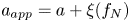 $a_{app} = a + \xi (f_N)$, inducing a decay of the apparent volume fraction of the suspension and, in fine, a decay of
  $\eta$ (Krieger Reference Krieger1972; Maranzano & Wagner Reference Maranzano and Wagner2001a). When the particle pressure increases more and overcomes the repulsive forces (
 $F_N \geqslant f_N^C$), the particles enter increasingly frequently into direct solid contact thanks to their asperities and the suspension passes from a frictionless state to a frictional one.
Interestingly, Mari et al. (Reference Mari, Seto, Morris and Denn2014) have shown that the onset of this frictionless–frictional transition (‘fft’) occurs for a critical shear stress (and not a shear rate,  $\dot {\gamma }$):
  $\sigma _{in}^{fft} \approx 0.3 \times f_N^C / (6{\rm \pi} a^2)$ for spheres, whose value is independent of
  $\phi$ as already observed in many experiments (Bender & Wagner Reference Bender and Wagner1996; Frith et al. Reference Frith, d'Haene, Buscall and Mewis1996; Maranzano & Wagner Reference Maranzano and Wagner2001a,Reference Maranzano and Wagnerb; Lootens et al. Reference Lootens, Van Damme, Hémar and Hébraud2005; Fall et al. Reference Fall, Lemaitre, Bertrand, Bonn and Ovarlez2010; Larsen et al. Reference Larsen, Kim, Zukoski and Weitz2010; Brown & Jaeger Reference Brown and Jaeger2012, Reference Brown and Jaeger2014). The authors have also shown that the stress range over which thickening occurs remains constant. This has motivated us to control the applied shear stress in the present study, instead of the shear rate. Once the load
  $F_N$ is large enough (
 $F_N \gg f_N^C$), the direct solid contacts between particles saturate since all the particles in the suspension have contacts with their neighbours: the system is in the frictional state. Mari et al. (Reference Mari, Seto, Morris and Denn2014) have measured the occurrence of this second regime at
  $\sigma _{out}^{fft} \sim f_N^C / a^2$.
In the frictional state, if  $\varSigma _{12}$ increases further, then a potential second shear-thinning regime can be observed. We want to emphasise that it is precisely this second shear-thinning regime (when the suspension is frictional) that will be explored in the present paper. The physical origin of this complex behaviour remains an open question. For instance, Acrivos, Fan & Mauri (Reference Acrivos, Fan and Mauri1994) suggested that the apparent shear-thinning behaviour observed in Couette flow can be due to a difference of density,
  $\varDelta \rho$, between the solid particles and the suspending fluid. Indeed, solid particles heavier than the suspending fluid settle because of gravity and form a more concentrated layer. Then, shear-induced viscous resuspension (Gadala-Maria Reference Gadala-Maria1979; Acrivos, Mauri & Fan Reference Acrivos, Mauri and Fan1993; Zarraga et al. Reference Zarraga, Hill and Leighton2000; Saint-Michel et al. Reference Saint-Michel, Manneville, Meeker, Ovarlez and Bodiguel2019; d'Ambrosio, Blanc & Lemaire Reference d'Ambrosio, Blanc and Lemaire2021) tends to homogenise the suspension when
  $\varSigma _{12}$ increases, which induces an apparent decay of the viscosity. However, while this mechanism may arise in some experiments with Couette rheometers, it cannot explain the shear-thinning behaviour observed in other types of flow. For instance, in the case of a parallel plates geometry, the shear-induced viscous resuspension would tend to increase the viscosity. In addition, we show that
  $\varSigma _{12}$ in the present study is large enough so that gravity would not cause significant deviation from uniform volume fraction, so the effect of any shear rate dependence related to gravity is absent.
Lastly, numerical simulations (Lobry et al. Reference Lobry, Lemaire, Blanc, Gallier and Peters2019) and experimental studies (Chatté et al. Reference Chatté, Comtet, Niguès, Bocquet, Siria, Ducouret, Lequeux, Lenoir, Ovarlez and Colin2018; Arshad et al. Reference Arshad, Maali, Claudet, Lobry, Peters and Lemaire2021; Le et al. Reference Le, Izzet, Ovarlez and Colin2023) have shown that the shear-thinning behaviour observed for concentrated viscous non-Brownian frictional suspensions (i.e. beyond the DST) could be related to a sliding friction between solid particles that varies with the normal force  $F_N$. Following the model from Brizmer, Kligerman & Etsion (Reference Brizmer, Kligerman and Etsion2007), Lobry et al. (Reference Lobry, Lemaire, Blanc, Gallier and Peters2019) have considered that the contact between particles is elastic and occurs only through a few hemisphere-like asperities. In these conditions and according to the Hertz theory, the elastic contact area
  $A_{contact}$ is proportional to
  $F_N^{2/3}$ which gives
 \begin{equation} \mu_s = \frac{F_T}{F_N} \propto \frac{A_{contact}}{F_N} \propto F_N^{{-}1/3}, \end{equation}
where  $F_T$ denotes the tangential force. This model is in good agreement with experimental works (Chatté et al. Reference Chatté, Comtet, Niguès, Bocquet, Siria, Ducouret, Lequeux, Lenoir, Ovarlez and Colin2018; Arshad et al. Reference Arshad, Maali, Claudet, Lobry, Peters and Lemaire2021; Le et al. Reference Le, Izzet, Ovarlez and Colin2023) which have directly determined the decay of
  $\mu _s$ with the normal force
  $F_N$ by conducting AFM measurements between pairs of particles. Arshad et al. (Reference Arshad, Maali, Claudet, Lobry, Peters and Lemaire2021) and Le et al. (Reference Le, Izzet, Ovarlez and Colin2023) have conducted AFM measurements to measure the pairwise friction between pairs of PS beads (
 $d \approx 40\ \mathrm {\mu } {\rm m}$) immersed in an aqueous liquid and silicone oil, respectively. Note that the system of suspension studied by Le et al. (Reference Le, Izzet, Ovarlez and Colin2023) is the same as that studied in the present paper. The different studies (Lobry et al. Reference Lobry, Lemaire, Blanc, Gallier and Peters2019; Arshad et al. Reference Arshad, Maali, Claudet, Lobry, Peters and Lemaire2021; Le et al. Reference Le, Izzet, Ovarlez and Colin2023) performed on suspensions of spherical particles have all converged to the following equation based on the works from Brizmer et al. (Reference Brizmer, Kligerman and Etsion2007):
 \begin{equation} \mu_s = \mu_s^\infty \times \text{coth}\left[ \mu_s^\infty \left( \frac{F_N}{L_c}\right)^m \right], \end{equation}
where  $L_c$ corresponds to the critical normal force which scales the saturation of
  $\mu _s$. In other words, the sliding friction coefficient becomes constant and equal to
  $\mu _s^\infty$ when
  $F_N \gg L_c$, because of an elastic to plastic transition of asperities deformation (Lobry et al. Reference Lobry, Lemaire, Blanc, Gallier and Peters2019). In the case of a contact between a perfectly smooth half sphere and a flat surface, Brizmer et al. (Reference Brizmer, Kligerman and Etsion2007) determined:
  $\mu _s^\infty = 0.27$ and
  $m = 0.35$, whereas Lobry et al. (Reference Lobry, Lemaire, Blanc, Gallier and Peters2019) estimated
  $L_c = 20 \ {\rm nN}$ based on the material properties (PS particles). More recently, Arshad et al. (Reference Arshad, Maali, Claudet, Lobry, Peters and Lemaire2021) directly measured
  $\mu _s^\infty = 0.18$ by AFM measurements and determined
  $L_c = 33.2 \ {\rm nN}$ and
  $m=0.54$ by fitting their experimental results obtained for PS particles in an aqueous liquid by (1.2). On the other hand, Le et al. (Reference Le, Izzet, Ovarlez and Colin2023) measured for PS beads in silicone oil:
  $\mu _s^\infty = 0.15$ (
 $m=0.4$). Note that, since the particles of the suspensions studied in the present paper are of the same chemical composition found in these studies from the literature (and even the same solvent for Le et al. Reference Le, Izzet, Ovarlez and Colin2023), we reuse (1.2) coupled with the latter constants to characterise the shear-thinning behaviour of the studied suspensions.
Lobry et al. (Reference Lobry, Lemaire, Blanc, Gallier and Peters2019) have numerically determined the relationship between the normal force applied on spherical particles and the shear stress:  $F_N = 6{\rm \pi} a^2 \varSigma _{12}/1.69$. Equivalently, a critical shear stress,
  $\varSigma _{c}$, can be defined as
  $L_{c} = 6{\rm \pi} a^2 \varSigma _c /1.69$, which allows one to obtain the following updated equation for the variable sliding friction coefficient:
 \begin{equation} \mu_s = \mu_s^\infty \times \text{coth}\left[ \mu_s^\infty \left( \frac{\varSigma_{12}}{\varSigma_c}\right)^m \right]. \end{equation}
 It is known in granular media that the two possible motions for a particle are sliding (characterised by  $\mu _s$) and rolling. The one offering the least resistance will be favoured but both can obviously occur at the same time in a sheared suspension (Estrada, Taboada & Radjai Reference Estrada, Taboada and Radjai2008). One can easily understand that the particle shape might have a significant effect on one or even both of these motions, depending on the contact between particles. A decade ago, the numerical simulations of Estrada et al. (Reference Estrada, Azéma, Radjai and Taboada2011) in granular media have shown that the way a non-spherical shape provides resistance to rolling can be essentially modelled by approximating the non-spherical particle (like a globular one) by a sphere ‘equipped’ with an apparent rolling resistance torque,
  $\varGamma _{F_N}$ (see figure 2). This shape-induced rolling resistance would be therefore characterised by a rolling friction coefficient,
  $\mu _r$, defined from a Coulomb-type law:
 \begin{equation} F_N^t \leqslant \mu_r F_N. \end{equation}
This is the sense in which we will consider rolling friction in the present paper. It is important to note that the main assumption that we make in the present paper is then to approximate the three-dimensional (3D) globular particles (irregular polyhedra) by their two-dimensional (2D)-projected shapes (irregular polygons).

Figure 2. Schema of rolling on a plane from the left to the right for a regular octagon (on the left) and a disc (on the right), thanks to a tangential force,  $\boldsymbol {F_T}$, applied at the centre of mass
  $G$ of the particles. The two particles have the same perimeter. The two systems can be considered equivalent if the disc is ‘equipped’ with a rolling resistance torque,
  $\varGamma _{F_N}$, directly related to a ‘rolling resistance force’,
  $\boldsymbol {F_{N}^t}$ defined from the normal force,
  $\boldsymbol {F_N}$, applied on
  $G$ as
  $F_N^t \leqslant \mu _r F_N$. Here,
  $\mu _r$ is the rolling friction coefficient (Estrada et al. Reference Estrada, Taboada and Radjai2008, Reference Estrada, Azéma, Radjai and Taboada2011).
Recent numerical simulations from Singh et al. (Reference Singh, Ness, Seto, de Pablo and Jaeger2020) have notably predicted a decay of  $\phi _m$ when
  $\mu _r$ increases, but a dearth of experimental data remains preventing verification of this important insight. Thus, in the present paper, after describing the experimental process in § 2, we first aim (in § 3) at measuring the jamming volume fraction,
  $\phi _m$, of the two studied suspensions, in order to characterise the rheological behaviour of non-Brownian viscous suspensions made of frictional particles with irregular shapes and compare it with the rheology of a basic suspension made of spheres of the same material. In the second part, we then determine by an image analysis process (see § 4) the rolling friction coefficient,
  $\mu _r$, of the studied globular particles in order to compare the numerical predictions of
  $\phi _m$ from the literature with our own experimental data.
2. Experimental methods
2.1. Suspensions
In this paper, the rheological behaviour of two different non-Brownian viscous suspensions are investigated. The two suspensions are very similar: they are both made of the same PS particles (TS40, Microbeads) with a density measured as  $\rho _p = 1.06 \ {\rm g}\ {\rm cm}^{-3}$ and sieved between
  $36$ and
  $45 \ \mathrm {\mu } {\rm m}$ in order to reduce the initially large size distribution, dispersed separately in the same solvent, a Newtonian silicone oil (Sigma-Aldrich) of density
  $\rho _f = 0.97 \ {\rm g}\ {\rm cm}^{-3}$ and viscosity
  $\eta _0 = 0.98 {\rm Pa}\ {\rm s}$ measured at
  $T=23\,^\circ {\rm C}$. To prepare a given suspension, a known mass of solid particles is carefully mixed with a known mass of liquid. The air bubbles are then removed by putting the sample in an ultrasound bath. The suspension is finally gently stirred in order to resuspend the particles that would have settled during the degassing procedure.
The only difference between the two suspensions remains in the shape of the PS particles. For the first suspension, labelled  $S_{PS40}$, the solid particles are spheres and to make the second suspension labelled
  $C_{PS40}$, the PS particles have been crushed by a process described in Appendix A. Figure 3 shows examples of these particles captured with a basic microscope: some spherical particles are presented in figure 3(a) whereas a sample of crushed particles is shown in figure 3(b). One can already note that the population of crushed particles is slightly heteroclyte, being composed of different shapes classified from simple spheres to more facetted particles and particles having both spherical and flat surfaces (see the rightmost schematic in figure 1). It is this appearance, combining spherical arcs and flat surfaces similarly to a quidditch ball (the so-called quaffle), which motivated us to choose the title for the present paper. Figure 4 displays an enlarged image of a sample of crushed PS particles, which allows one to better appreciate this heteromorphism.

Figure 3. (a) Spherical PS particles. (b) Crushed PS particles. Scale 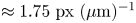 $\approx 1.75\ {\rm px}\ (\mathrm {\mu }{\rm m})^{-1}$. Particle diameter:
  $d = 2a \sim 40\ \mathrm {\mu } {\rm m}$.

Figure 4. Globular/crushed PS particles composing  $C_{PS40}$.
A quantitative study by image analysis has been conducted over a few hundred images captured with a microscope such as those presented in figure 3 in order to characterise the size distribution of the two types of particles, displayed in figure 5. One can observe that the spherical and crushed PS particles have roughly the same size, and both populations can be considered monodisperse with mean and standard deviation of the diameter of  $\langle d \rangle ^{S_{PS40}} \approx (42 \pm 1) \ \mathrm {\mu } {\rm m}$ and
  $\langle d \rangle ^{C_{PS40}} \approx (43 \pm 4) \ \mathrm {\mu } {\rm m}$. If the crushed particles appear slightly larger than the spherical particles, it is likely due to the fact that the diameter
  $d$ is calculated from the projected area of the particle.

Figure 5. Size distribution of spheres (blue) and crushed particles (orange). For a crushed particle, the projected area, denoted  $A_p$, is measured by microscopic image analysis. The diameter
  $d$ corresponds to the diameter of a disc having the same area as the projected crushed particle:
  $d = 2 \times \sqrt {A_{p}/{\rm \pi} }$.
2.2. Rheometry experiments
Rheometric experiments are carried out in a controlled-stress rheometer HR30 (TA instruments) with a smooth rotating parallel plate of radius  $R=20 \ {\rm mm}$. The temperature is controlled by the static lower plate and is set at
  $T = 23\,^\circ {\rm C}$ for all the experiments. The gap is imposed at
  $1 \ {\rm mm} \lesssim h \lesssim 2 \ {\rm mm}$, which allows one to have enough particles (
 $20 \lesssim h/d \lesssim 50$) to minimise phenomena of layering and sliding. The preference of working in a parallel rotating disc is led by the near absence of shear-induced particle migration in such a geometry (Chow et al. Reference Chow, Sinton, Iwamiya and Stephens1994; Merhi et al. Reference Merhi, Lemaire, Bossis and Moukalled2005), which helps in keeping a homogeneous suspension across the gap. However, the drawback of this geometry is that the shear rate is not constant. Indeed,
  $\dot {\gamma }$ increases from 0 at the centre to
  $\dot {\gamma }_R = \varOmega R / h$ at
  $r=R$, with
  $\varOmega$ the angular velocity of the upper rotating plate. In the case of a non-Newtonian behaviour, this variation can be problematic since the viscosity of the suspension,
  $\eta$, depends on the shear rate,
  $\dot {\gamma }$. In order to take into account this experimental bias and deduce the correct values of
  $\eta$, we use the well-known Mooney–Rabinowitsch correction:
 \begin{equation} \eta = \eta_{app}\left[ 1 + \frac{1}{4}\frac{\text{d} \ln(\eta_{app})}{\text{d} \ln(\dot{\gamma}_{R})}\right], \end{equation}
where  $\eta _{app}$ is the apparent viscosity deduced by the rheometer from the measurements of shear rate at the rim of parallel plates,
  $\dot {\gamma }_R$, and applied torque,
  $\varGamma$,
 \begin{equation} \eta_{app} = \frac{2}{{\rm \pi} R^3}\frac{\varGamma}{\dot{\gamma}_R}. \end{equation}
 We studied the rheological behaviour of each suspension over a wide range of shear stress,  $\varSigma _{12} \in [5, 100] \ {\rm Pa}$, and solid volume fraction,
  $\phi \in [0.43, 0.51]$. Note that we work with a volume-imposed geometry and being sure of the volume fraction
  $\phi$ present in the gap is critical for our experiments. It is very difficult to prepare a proper sample with a known volume fraction when
  $\phi$ is close to the jamming volume fraction,
  $\phi _m$. This could be due to the presence of air bubbles hard to remove, instantaneous shear-induced migration when the sample is poured into the gap or even a yield stress which may prevent the suspension from flowing into the gap by gravity. For these reasons, the maximum value for
  $\phi$ in the experiments was kept at 0.51. For each
  $\varSigma _{12}$ and each
  $\phi$ (in total,
  $50$ combinations of
  $(\phi, \varSigma _{12})$), a shear reversal experiment was performed. We encourage the readers to consult Blanc et al. (Reference Blanc, d'Ambrosio, Lobry, Peters and Lemaire2018) for details on the protocol. Briefly, the suspension is simply sheared at a given constant
  $\varSigma _{12}$. Once the steady state has been reached (
 $\eta$ is constant), the flow direction is reversed while the value of
  $\varSigma _{12}$ is kept constant. Then, the suspension is sheared in this new direction until the steady value of
  $\eta$ is retrieved. For each
  $\phi$ on both types of suspension, a series of shear-reversal experiments was performed on two independent samples. The results in the following correspond to the average of these two independent measurements.
Within these conditions, the values of the Péclet and Reynolds numbers characterise the suspension as non-Brownian and its flow as viscous (inertial effects are negligible), respectively:
 \begin{equation} Pe = \frac{6{\rm \pi}\varSigma_{12} a^3}{k_B T} > 10^8 \quad \text{and} \quad Re = \frac{\rho_f \varSigma_{12} h^2}{\eta_0^2} < 0.1, \end{equation}
with  $k_B$ the Boltzmann constant. At the same time, note that the Stokes number is kept small throughout all the experiments:
  $St = (\frac {1}{18}){\rho _p d^2 \varSigma _{12}}/{\eta ^2} < 10^{-5}$. It is thus expected that only viscous and contact forces govern the suspension behaviour.
The maximum shear stress ( $\varSigma _{12} = 100 \ {\rm Pa}$) is set by the occurrence of edge fracture which is expected for a first normal stress of the order of the capillary pressure (Keentok & Xue Reference Keentok and Xue1999):
  $N_1 \approx 2\gamma _{{air\text {-}oil}}/h$, with the surface tension of silicone oil,
  $\gamma _{{air\text {-}oil}} \approx 30 \ {\rm mN}\ {\rm m}^{-1}$. Since the literature shows
  $N_1 \lesssim 0.5 \varSigma _{12}$, we obtain the following criterion to avoid edge fracture:
  $\varSigma _{12} \lesssim 120 \ {\rm Pa}$, a value close to experimental observations. On the other hand, the minimum stress (
 $\varSigma _{12} = 5 \ {\rm Pa}$) is chosen in such a way that the Shield number, denoted
  $Sh$, is large enough (
 $Sh \gg 1$) to ensure that the particles do not settle due to the slight difference of density,
  $\Delta \rho$, between the solid and liquid phases, and that a vertical homogeneous suspension is maintained throughout the entire experimental procedure:
 \begin{equation} Sh = \frac{\varSigma_{12}}{\Delta\rho g d} \gtrsim 10^{2} \quad \text{with} \ \Delta\rho = \rho_p - \rho_f = (0.09 \pm 0.02) \ {\rm g} \ {\rm cm}^{{-}3}. \end{equation}
We want to underline that AFM measurements found in the literature (Le et al. Reference Le, Izzet, Ovarlez and Colin2023) do not observe any repulsive forces before contact for PS particles (also from Microbeads) in a silicone oil (from Merck,  $\rho _f = 0.95 \ {\rm g}\ {\rm cm}^{-3}$,
  $\eta _0 \approx 20 \ {\rm mPa} \ {\rm s}$ at
  $25\,^\circ {\rm C}$), meaning that we are already in the frictional regime for the range of
  $\varSigma _{12}$ studied in the present paper, and that particles are in contact even when
  $\dot {\gamma } \rightarrow 0$. This will be confirmed later by the measured values of
  $\phi _m$ and the comparison with the literature (Gallier et al. Reference Gallier, Lemaire, Peters and Lobry2014; Mari et al. Reference Mari, Seto, Morris and Denn2014; Peters et al. Reference Peters, Ghigliotti, Gallier, Blanc, Lemaire and Lobry2016).
To conclude this section on the rheometry, we want to emphasise that the plate surfaces are smooth and we made sure that there was no wall slip phenomenon by measuring the viscosity of the suspensions at the largest volume fraction for different gap size. A viscosity found to be independent of the height of the upper plate indicates that there is no detectable wall slip (Yoshimura & Prud'homme Reference Yoshimura and Prud'homme1988).
3. Results and discussion on macroscopic rheological measurements
3.1. Rheological measurements
In this section, we aim to characterise the rheological behaviour of the suspension made of crushed PS particles ( $C_{PS40}$) and compare it with our measurements of the rheology of the suspension made of spherical PS particles (
 $S_{PS40}$), which is more common in the literature.
3.1.1. Steady viscosity
Figure 6 displays the variation of the measured relative steady viscosity,  $\eta _r = \eta /\eta _0$, with applied shear stress,
  $\varSigma _{12}$, for (a) the suspension
  $S_{PS40}$ made of spherical PS particles and (b)
  $C_{PS40}$ made of crushed PS particles. Each coloured point corresponds to an experimental measurement of
  $\eta _r$ (relative viscosity corrected by (2.1)) at a given
  $\phi$ and a given
  $\varSigma _{12}$. The relative uncertainty for each measurement, not represented on the graphs in figure 6 in order to keep them clear, is always smaller than 5 %.

Figure 6. Variation of the measured relative steady viscosity,  $\eta _r = \eta /\eta _0$, with applied shear stress
  $\varSigma _{12}$ for(a) the suspension
  $S_{PS40}$ made of spherical PS beads and (b)
  $C_{PS40}$ made of crushed PS particles. Each colour labels a solid volume fraction
  $\phi$: 0.43 (blue), 0.45 (orange), 0.47 (green), 0.49 (red) and 0.51 (purple). For each given
  $\phi$, the experimental measurements (coloured dot) are fitted by a power law (coloured straight line):
  $\varSigma _{12} = K \dot {\gamma }^n$ with
  $\dot {\gamma } = \varSigma _{12}/\eta$. The resulting parameters of these fits are shown in figure 8.
The values of viscosity measured on  $S_{PS40}$ within the explored range of
  $\varSigma _{12}$ are in quite good agreement with other previous works present in the literature (Blanc et al. Reference Blanc, d'Ambrosio, Lobry, Peters and Lemaire2018; Lobry et al. Reference Lobry, Lemaire, Blanc, Gallier and Peters2019; Le et al. Reference Le, Izzet, Ovarlez and Colin2023) and conducted on an identical system (i.e. PS spheres of size close to
  $40\ \mathrm {\mu } {\rm m}$ dispersed in silicone oil). It appears in figure 6 that
  $C_{PS40}$ exhibits a rheological behaviour which is broadly similar to that which characterises
  $S_{PS40}$. In particular, we observe for both suspensions that:
(i) as expected,
 $\eta _r$ increases with $\phi$ for a given $\varSigma _{12}$;
(ii)
$\eta _r$ decreases with $\varSigma _{12}$ for a given $\phi$, qualifying the non-Newtonian behaviour in the range of applied shear stress ($\varSigma _{12} \in [5\unicode{x2013}100] \ {\rm Pa}$) for both suspensions as shear-thinning;(iii) as expected, the decay of
$\eta _r$ with $\varSigma _{12}$ is steeper (meaning the shear-thinning behaviour is more pronounced) at large $\phi$.


On the other hand, the primary distinction between the suspensions is that the shear-thinning behaviour is stronger for  $C_{PS40}$ compared with
  $S_{PS40}$ for a given
  $\phi$. Figure 7 displays the normalised difference of relative viscosity between the two suspensions,
  $(\eta _r^{C_{PS40}} - \eta _r^{S_{PS40}}) / \eta _r^{S_{PS40}}$, as function of the applied shear stress
  $\varSigma _{12}$. One can then easily observe that the suspension made of crushed particles is more viscous than the suspension made of spherical particles at low shear stress, whereas the viscosities of the two suspension are nearly the same at high shear stress.

Figure 7. Variation of the measured relative steady viscosity difference between  $C_{PS40}$ and
  $S_{PS40}$,
  $\eta _r^{C_{PS40}} - \eta _r^{S_{PS40}}$, normalised by the measured relative steady viscosity for the suspension made of spherical PS particles,
  $\eta _r^{S_{PS40}}$, as function of the applied shear stress
  $\varSigma _{12}$. Each colour labels the solid volume fraction
  $\phi$: 0.43 (blue), 0.45 (orange), 0.47 (green), 0.49 (red) and 0.51 (purple).
According to the literature (Coussot & Piau Reference Coussot and Piau1994; Schatzmann, Fischer & Bezzola Reference Schatzmann, Fischer and Bezzola2003; Sosio & Crosta Reference Sosio and Crosta2009; Mueller, Llewellin & Mader Reference Mueller, Llewellin and Mader2010; Vance, Sant & Neithalath Reference Vance, Sant and Neithalath2015), we can quantify the non-Newtonian behaviour of such suspensions by fitting the experimental measurements by a power law (coloured straight lines in figure 6):
 \begin{equation} \varSigma_{12} = K \dot{\gamma}^n, \end{equation}
where  $K$ and
  $n$ are the consistency factor and the shear-thinning index, respectively. Their values resulting from the fits of the experimental data in figure 6 are displayed as functions of
  $\phi$ in figure 8. We observe in figure 8(a) that
  $K$ increases with
  $\phi$ as expected. This reflects the increase of the viscosity with volume fraction. On the other hand, we observe in figure 8(b) that
  $n$ decreases with
  $\phi$, which accounts for the more pronounced shear-thinning behaviour at large
  $\phi$. One can also note that
  $n$ is systematically smaller in the case of
  $C_{PS40}$ at a given
  $\phi$, which reflects the more pronounced shear-thinning behaviour for the suspension made of crushed particles. More precisely, we observe that the relative variation of
  $n$ over the range of studied
  $\phi$ is roughly twice as large for
  $C_{PS40}$ than for
  $S_{PS40}$ (
 ${\Delta n}/{\langle n\rangle } \sim 0.2$ for crushed particles whereas
  ${\Delta n}/{\langle n\rangle } \sim 0.1$ for spheres). Regarding the consistency factor,
  $K$, it is interesting to see that apparently
  $K^{C_{PS40}} \approx K^{S_{PS40}}$ at a given
  $\phi$. However, any further interpretation of this comparison in
  $K$ can be difficult since its units are not exactly the same between the two suspensions because
  $n^{C_{PS40}} \ne n^{S_{PS40}}$ (
 $[K] = {\rm Pa} \ {\rm s}^{n}$).

Figure 8. Variation of (a) the consistency factor  $K$ and (b) the shear-thinning index
  $n$ with solid volume fraction
  $\phi$ for the suspensions
  $S_{PS40}$ made of spherical PS particles (blue discs) and
  $C_{PS40}$ made of crushed PS particles (orange squares), deduced from (3.1).
From figures 6 and 8, it can be seen that the more pronounced shear-thinning behaviour which characterises the suspension  $C_{PS40}$ compared with the same suspension made of spheres (
 $S_{PS40}$) results from the observations that
  $\eta _r^{C_{PS40}} \approx \eta _r^{S_{PS40}}$ at large
  $\varSigma _{12}$ whereas
  $\eta _r^{C_{PS40}} > \eta _r^{S_{PS40}}$ at small
  $\varSigma _{12}$.
To conclude this section, we discuss why we have not considered the existence of a yield stress for either suspension. It is true that it is more relevant to characterise the rheological behaviour for some non-Brownian suspensions by using the Herschel–Bulkley (H-B) law:
 \begin{equation} \varSigma_{12} = \tau_c + K \dot{\gamma}^n \end{equation}
instead of (3.1). According to the literature (Pantina & Furst Reference Pantina and Furst2005; Guy et al. Reference Guy, Richards, Hodgson, Blanco and Poon2018; Richards et al. Reference Richards, Guy, Blanco, Hermes, Poy and Poon2020), it is known that the existence of a yield stress,  $\tau _c$, may be caused by the presence of weak adhesive forces between solid particles which would lead to particle aggregation. Thus, the value of
  $\tau _c$ may be understood as the minimum stress required to break these aggregates. Furthermore, it is expected that the crushed particles, which have some flat faces, favour Van der Waals interactions since they offer a much larger contacting surface between particles compared with spheres, leading to a higher yield stress. In view of this, we have also fitted our experimental measurements in figure 6 by (3.2). The results have shown that the impact of the third fitting parameter
  $\tau _c$ on
  $K$ and
  $n$ is negligible, since we found
  $\tau _c < 1 \ {\rm Pa}$ for both suspensions and all explored
  $\phi$. For
  $S_{PS40}$, one can note that this is in good agreement with the works of Le et al. (Reference Le, Izzet, Ovarlez and Colin2023) who measured
  $\tau _c=0.3 \ {\rm Pa}$ for a very dense suspension made of PS beads having a size of
  $40\ \mathrm {\mu } {\rm m}$ and concentration
  $\phi =0.55$ in a silicone oil (the same system as studied in the present paper). The largest volume fraction studied in the present work being
  $\phi =0.51$, one can expect that the values of
  $\tau _c$ for
  $S_{PS40}$ are even smaller than this value within the range of studied
  $\phi$. Thus, we can advance with enough confidence that the minimum applied shear stress in our study (
 $\varSigma _{12} = 5 \ {\rm Pa}$) is at least 10 times larger than
  $\tau _c$ for
  $S_{PS40}$ and
  $C_{PS40}$. We confirm by some measurements from the shear-reversal experiments that adhesive forces do not play a significant role in the rheological behaviour of the studied suspensions within the applied range of shear stress
  $\varSigma _{12}$.
3.1.2. A stress-dependent jamming volume fraction
We want to recall that the shear-thinning regime observed for a frictional non-Brownian suspension is common and has already been observed extensively in the literature for suspensions made of spheres (Gadala-Maria & Acrivos Reference Gadala-Maria and Acrivos1980; Zarraga et al. Reference Zarraga, Hill and Leighton2000; Dbouk et al. Reference Dbouk, Lobry and Lemaire2013; Vázquez-Quesada et al. Reference Vázquez-Quesada, Tanner and Ellero2016, Reference Vázquez-Quesada, Mahmud, Dai, Ellero and Tanner2017) or even facetted (sugar) particles (Blanc et al. Reference Blanc, d'Ambrosio, Lobry, Peters and Lemaire2018). As explained in the introduction of the present paper, the physical origin of this complex behaviour remains an open question. Some recent works, including an experimental study from Chatté et al. (Reference Chatté, Comtet, Niguès, Bocquet, Siria, Ducouret, Lequeux, Lenoir, Ovarlez and Colin2018) and numerical simulations from Lobry et al. (Reference Lobry, Lemaire, Blanc, Gallier and Peters2019), have demonstrated that the shear-thinning behaviour for frictional spheres could come from a decay of the sliding friction coefficient,  $\mu _s$, when the shear stress,
  $\varSigma _{12}$, increases, which induces an increase of the jamming volume fraction,
  $\phi _m$ (Wildemuth & Williams Reference Wildemuth and Williams1984; Zhou, Uhlherr & Luo Reference Zhou, Uhlherr and Luo1995; Blanc et al. Reference Blanc, d'Ambrosio, Lobry, Peters and Lemaire2018; Lobry et al. Reference Lobry, Lemaire, Blanc, Gallier and Peters2019; Gilbert et al. Reference Gilbert, Valette and Lemaire2022). The introduction of a stress-dependent jamming fraction
  $\phi _m(\varSigma _{12})$ is thus very useful to describe accurately the complex rheological behaviour of a suspension. Figure 9 displays the evolution of
  $\eta _r$ with
  $\phi$ for each applied
  $\varSigma _{12}$ (see colour code). The coloured points correspond to the experimental data and, for each applied
  $\varSigma _{12}$, the variation of the reduced viscosity,
  $\eta _r$, with the volume fraction,
  $\phi$, is fitted by a Maron–Pierce-type law:
 \begin{equation} \eta_r = \frac{\alpha_0}{\left( 1 - \dfrac{\phi}{\phi_m(\varSigma_{12})} \right)^2} . \end{equation}
Note that the parameter  $\alpha _0$ in (3.3) is used in order to get an accurate fit of our experimental data. If one were to apply (3.3) over the full range of particle volume fractions,
  $\alpha _0$ would need to be 1 in order that
  $\eta _r=1$ when
  $\phi \rightarrow 0$. However, this fit only works in the dense regime, typically for
  $\phi \gtrsim 0.3$ in the case of frictional spherical particles, and hence
  $\alpha _0$ can have a value different from 1 in order to describe the variation of
  $\eta _r$ with
  $\phi$ accurately within this regime (Lobry et al. Reference Lobry, Lemaire, Blanc, Gallier and Peters2019). In our case, a very good fit for each applied shear stress (plotted as coloured lines in figure 9) is obtained for
  $\alpha _0 = 0.85$ for both suspensions, a value not too far from the one used in the original equation of Maron & Pierce (Reference Maron and Pierce1956):
  $\alpha _0 = 1$ when
  $\phi _m \approx 0.64$. The value chosen here is also in good agreement with the numerical simulations of Lobry et al. (Reference Lobry, Lemaire, Blanc, Gallier and Peters2019) who have found that
  $0.65 \lesssim \alpha _0 \lesssim 1$ when
  $0 \lesssim \mu _s \lesssim 2$, which are the typical values of
  $\mu _s$ for common materials such as PS (Arshad et al. Reference Arshad, Maali, Claudet, Lobry, Peters and Lemaire2021; Le et al. Reference Le, Izzet, Ovarlez and Colin2023), polymethyl methacrylate, glass and rubber. In figure 9(b), we can observe that it satisfactorily fits the experimental data for crushed particles.

Figure 9. Variation of measured relative steady viscosity  $\eta _r$ with solid volume fraction
  $\phi$ for suspensions (a)
  $S_{PS40}$ made of spherical PS and (b)
  $C_{PS40}$ made of crushed PS particles. Each colour labels the applied shear stress
  $\varSigma _{12}$: 5 (blue), 10 (orange), 15 (green), 20 (red), 28 (purple), 36 (brown), 45 (pink), 60 (grey), 80 (yellow) and 100 (cyan). For each given
  $\varSigma _{12}$, the experimental measurements (coloured dot) are fitted by a Maron–Pierce-type law (see (3.3)). The measurements of
  $\phi _m(\varSigma _{12})$ resulting from these fits are shown in figure 10.
The good fit obtained with this given value of  $\alpha _0$ for both suspensions is not so surprising as it is known that the values of
  $\eta _r$ when
  $\phi \rightarrow \phi _m$ are controlled primarily by the value of
  $\phi _m$ (Blanc et al. Reference Blanc, d'Ambrosio, Lobry, Peters and Lemaire2018; Lobry et al. Reference Lobry, Lemaire, Blanc, Gallier and Peters2019). Figure 10 displays the variation of
  $\phi _m$ with
  $\varSigma _{12}$, determined by (3.3) with
  $\alpha _0 = 0.85$ for the suspensions
  $S_{PS40}$ made of PS beads (blue circle) and
  $C_{PS40}$ made of crushed particles (orange squares). As expected, we observe that
  $\phi _m$ increases with
  $\varSigma _{12}$ for both suspensions. This increase is larger for
  $C_{PS40}$ when compared with
  $S_{PS40}$, which illustrates the more pronounced shear-thinning behaviour for the suspension made of crushed particles. To be precise, we observe that
  $\phi _m^{C_{PS40}} < \phi _m^{S_{PS40}}$ within the smaller end of the
  $\varSigma _{12}$ range whereas
  $\phi _m^{C_{PS40}} \approx \phi _m^{S_{PS40}}$ at the largest
  $\varSigma _{12}$ values. This mirrors the previous observation made from the viscosity comparison between the two suspensions.

Figure 10. Variation of the jamming fraction  $\phi _m$ with shear stress
  $\varSigma _{12}$ for the suspensions
  $S_{PS40}$ made of spheres PS (blue circle) and
  $C_{PS40}$ made of crushed PS particles (orange square), deduced from figure 9 and (3.3) with
  $\alpha _0 = 0.85$. The coloured area for each suspension is related to the possible range of
  $\alpha _0$:
  ${0.65 \lesssim \alpha _0 \lesssim 1}$.
It is easy to understand that the values of  $\phi _m$ determined by (3.3) might depend slightly on the value of
  $\alpha _0$, and hence we have also fitted our experimental data of
  $\eta _r(\phi )$ by (3.3) with the two known extreme values of
  $\alpha _0$ (Lobry et al. Reference Lobry, Lemaire, Blanc, Gallier and Peters2019):
  $\alpha _0 = 0.65$ and
  $\alpha _0 = 1$ (the corresponding curves are not plotted in figure 9 in order to keep the graph clear). The confidence areas plotted in figure 10 for each suspension represent this influence of
  $\alpha _0$ on
  $\phi _m$. Thus, one can observe that the values of
  $\phi _m$ for
  $S_{PS40}$ are between
  $0.560 \pm 0.005$ and
  $0.595 \pm 0.009$ in very good agreement with Lobry et al. (Reference Lobry, Lemaire, Blanc, Gallier and Peters2019), whereas they are between
  $0.550 \pm 0.004$ and
  $0.595 \pm 0.009$ for
  $C_{PS40}$. It is quite satisfying that these values of
  $\phi _m$ for both types of suspension are globally in very good agreement with the literature when non-Brownian frictional (
 $\mu _s \ne 0$) suspensions are considered (Zarraga et al. Reference Zarraga, Hill and Leighton2000; Ovarlez et al. Reference Ovarlez, Bertrand and Rodts2006; Boyer et al. Reference Boyer, Guazzelli and Pouliquen2011; Mari et al. Reference Mari, Seto, Morris and Denn2014; Peters et al. Reference Peters, Ghigliotti, Gallier, Blanc, Lemaire and Lobry2016; Singh et al. Reference Singh, Mari, Denn and Morris2018; Lobry et al. Reference Lobry, Lemaire, Blanc, Gallier and Peters2019; Singh et al. Reference Singh, Ness, Seto, de Pablo and Jaeger2020). Furthermore, it is noteworthy that the primary observations that the jamming volume fraction
  $\phi _m$ is smaller in the case of non-spherical particles at low shear stress whereas the rheological behaviours of non-spherical and spherical particles are characterised by the same
  $\phi _m$ at high shear stress is not altered by the value of
  $\alpha _0$ within its known range.
The rest of the paper focuses on finding a physical mechanism to explain the observed rheological difference between the suspension made of crushed particles and the suspension made of spheres.
3.2. Physical origin of the stronger shear-thinning regime for crushed particles
In this section, we want to understand the physical origin of the higher viscosity in the suspension of crushed particles ( $C_{PS40}$) for small shear stress, as well as the reason that the viscosity of the two types of suspension are similar when
  $\varSigma _{12}$ is increased. Since the only difference between the suspensions is the shape of particles present in them, it is obvious that this difference in viscosity is related to it. Two different possible physical origins will be thus investigated. First, we show in § 3.2.1 that it is unlikely that the small remaining adhesion between particles (which is expected to be stronger for the crushed particles at a given shear stress) explains this observation. Second, we discuss in §§ 3.2.2 and 3.2.3 whether changes in viscosity can be explained by a variable sliding friction between particles coupled with a rolling resistance of particles related to the particle shape itself. To end this section, we study in § 3.2.4 the rheological behaviour of the suspensions in a frictionless case in order to confirm some assumptions of the considered model.
3.2.1. Shear reversal experiments and absence of adhesion
As mentioned previously in this paper, shear-thinning behaviour of a suspension is common and can have different possible physical origins depending on the studied system (Gadala-Maria & Acrivos Reference Gadala-Maria and Acrivos1980; Zarraga et al. Reference Zarraga, Hill and Leighton2000; Dbouk et al. Reference Dbouk, Lobry and Lemaire2013; Vázquez-Quesada et al. Reference Vázquez-Quesada, Tanner and Ellero2016, Reference Vázquez-Quesada, Mahmud, Dai, Ellero and Tanner2017; Blanc et al. Reference Blanc, d'Ambrosio, Lobry, Peters and Lemaire2018; Chatté et al. Reference Chatté, Comtet, Niguès, Bocquet, Siria, Ducouret, Lequeux, Lenoir, Ovarlez and Colin2018; Lobry et al. Reference Lobry, Lemaire, Blanc, Gallier and Peters2019; Gilbert et al. Reference Gilbert, Valette and Lemaire2022). One of them is adhesion. Weak adhesive forces exist between solid particles that would lead to particle aggregation. In this scenario, two main features would appear. First, a suspension would exhibit a yield stress  $\tau _c$ (Brown et al. Reference Brown, Forman, Orellana, Zhang, Maynor, Betts, DeSimone and Jaeger2010), which may be understood as the minimum stress needed to break these aggregates. Second, they would exhibit shear-thinning behaviour, related to the fact that increasing
  $\varSigma _{12}$ would break more and more aggregates, which would produce as a result a decrease in the viscosity of the suspension. Furthermore, this explanation would be suitable to explain the highest viscosity at low
  $\varSigma _{12}$ for crushed particles while the viscosity of the two types of suspensions (
 $S_{PS40}$ and
  $C_{PS40}$) would tend to be similar at large
  $\varSigma _{12}$. As already mentioned previously in § 3.1.1, flat surfaces of crushed particles favour particle adhesion. Potential aggregates are then less likely to be destroyed in
  $C_{PS40}$ than in
  $S_{PS40}$ when both suspensions are sheared at a given small enough
  $\varSigma _{12}$. This would make
  $C_{PS40}$ more viscous than
  $S_{PS40}$ when
  $\varSigma _{12}$ is small. In contrast, when
  $\varSigma _{12} \gg \tau _c$, all the aggregates are destroyed by shear, even in the case of
  $C_{PS40}$ which then flows similarly to
  $S_{PS40}$.
The first flaw in this explanation has already been presented in § 3.1.1. Indeed, we have seen that the smallest value of  $\varSigma _{12}$ that we apply to shear the suspension is at least 10 times larger than
  $\tau _c$. At
  $\varSigma _{12} = 10\ {\rm Pa}$ (second lowest value of applied shear stress), we have
  $\varSigma _{12} \gtrsim 20 \times \tau _c$. Yet, a significant difference of viscosity between the two suspensions still remains at large
  $\phi$, which raises doubt that adhesion could be the main physical origin of the stronger shear-thinning for
  $C_{PS40}$. For instance, at
  $\phi = 0.51$ and
  $\varSigma _{12} = 10\ {\rm Pa}$,
  $\eta _r = (110 \pm 5) \ {\rm Pa} \ {\rm s}$ for
  $C_{PS40}$ whereas
 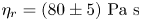 $\eta _r = (80 \pm 5) \ {\rm Pa} \ {\rm s}$ for
  $S_{PS40}$ (see figure 9), which gives a difference of the order of
  $30\,\%$. Nevertheless, we understand that this argument about
  $\varSigma _{12}$ and
  $\tau _c$ alone is insufficient to support the statement that the adhesion is not mainly responsible for the more pronounced shear-thinning for
  $C_{PS40}$. It is indeed very difficult to estimate precisely when the adhesive forces can be neglected only from
  $\tau _c$. To go further, we have conducted a series of shear-reversal experiments on both types of suspension by following the procedure of Blanc et al. (Reference Blanc, d'Ambrosio, Lobry, Peters and Lemaire2018).
A shear-reversal experiment may turn out to be very interesting. It is a very basic experiment (the suspension is simply sheared at a given  $\varSigma _{12}$ in a given direction before the flow direction is reversed whereas
  $\varSigma _{12}$ is kept constant), characterised by a very specific transient response of
  $\eta$ which has been observed in all shear reversal experiments (Gadala-Maria & Acrivos Reference Gadala-Maria and Acrivos1980; Blanc et al. Reference Blanc, Peters and Lemaire2011a) and in simulations (Ness & Sun Reference Ness and Sun2016; Peters et al. Reference Peters, Ghigliotti, Gallier, Blanc, Lemaire and Lobry2016). Figure 11 displays an example of the transient response of
  $\eta$ for
  $S_{PS40}$ (in blue) and
  $C_{PS40}$ (in orange) at
  $\varSigma _{12}=10 \ {\rm Pa}$ and
  $\phi = 0.51$. As can be observed, a step-like drop of
  $\eta$ occurs just after the shear reversal and the viscosity of the suspension reaches a minimum value,
  $\eta _{min}$, at a strain
  $\gamma = \gamma _{min}$ (
 $\gamma =0$ corresponds to the moment of reversal). This drop is then followed by a rebound of the viscosity which reaches the steady value,
  $\eta _s = \eta _0\eta _r$, it had before the shear reversal, over an accumulated strain,
  $\gamma$, roughly equal to
  $\gamma _s \sim 10$. Interestingly, the numerical simulations from Ness & Sun (Reference Ness and Sun2016) and Peters et al. (Reference Peters, Ghigliotti, Gallier, Blanc, Lemaire and Lobry2016) have shown that the hydrodynamic and contact contribution to the viscosity, denoted respectively
  $\eta ^H$ and
  $\eta ^C$, are connected directly to the values of
  $\eta$ and
  $\eta _{min}$. More precisely, with
  $\eta _s = \eta ^H + \eta ^C$, Peters et al. (Reference Peters, Ghigliotti, Gallier, Blanc, Lemaire and Lobry2016) have numerically shown in the case of a non-Brownian suspension made of (frictional or frictionless) beads the following relations:
 \begin{equation} \eta^C = \frac{\eta_s - \eta_{min}}{0.85/\eta_0} \quad {\rm and} \quad \eta^H = \frac{\eta_{min} - 0.15 \eta_s}{0.85/\eta_0} . \end{equation}
Roughly,  $\eta ^H \sim \eta _{min}/\eta _0$ and
  $\eta ^C \sim (\eta _s - \eta _{min})/\eta _0$. We refer readers to the numerical work of Peters et al. (Reference Peters, Ghigliotti, Gallier, Blanc, Lemaire and Lobry2016) to better understand the physical origin of this result. In brief, the particles in contact tend to separate when the shear is reversed. The microstructure of the suspension is thus broken, which induces the drop of the viscosity. Progressively, the microstructure of the suspension is then rebuilt (mirroring the microstructure before the shear reversal since the flow direction has been reversed), which induces the rebound of
  $\eta$ to its steady value.

Figure 11. Example of transient viscosity response as a function of the accumulated strain  $\gamma$ during a shear reversal experiment for
  $S_{PS40}$ (in blue) and
  $C_{PS40}$ (in orange) with
  $\varSigma _{12} = 10 \ {\rm Pa}$ and
  $\phi =0.51$.
  $\gamma = 0$ corresponds to the moment when the flow is reversed. Inset: Enlarged view to better visualise the minimum value of viscosity,
  $\eta _{min}$ reached during the transient when
  $\gamma = \gamma _{min}$.
In the present study, the transient viscosity induced by a shear reversal can be very interesting because, if a stress-dependent particle aggregation occurs, then it should also affect the values of  $\eta _{min}$ and the characteristic strains,
  $\gamma$. Notably, Gilbert (Reference Gilbert2021) has studied the rheology of a non-Brownian frictional suspension composed of homemade soft PDMS particles (Young modulus,
  $E_{PDMS} = 1.8 \ {\rm MPa} \ll E_{PS} \sim 3 \ {\rm GPa}$) suspended in Span 80 (Newtonian liquid). By using the JKR theory (Johnson, Kendall & Roberts Reference Johnson, Kendall and Roberts1971), the author has observed for this suspension that adhesion plays a role if
  $\varSigma _{12} \lesssim \tau _a \approx 10 \ {\rm Pa}$. By doing shear reversal experiments, he has then shown (see figures 86-2 of Gilbert Reference Gilbert2021) that
  $\eta _{min}^{\varSigma _{12} < \tau _a} \gg \eta _{min}^{\varSigma _{12} > \tau _a}$, and that the characteristic deformation of the transient response for a shear reversal,
  $\gamma _s$, was much larger than 10 (
 $\gamma _s \sim 50$ for
  $\phi =0.4$ and
  $\varSigma _{12} = \tau _a$ in the case of his suspension).
Figure 12 displays the experimental measurements (coloured symbols) of  $\eta _{min}/\eta _0$ within the studied range of
  $\varSigma _{12}$ for (a)
  $S_{PS40}$ and (b)
  $C_{PS40}$, and one can see it is not similar to what has been observed by Gilbert (Reference Gilbert2021) for a non-Brownian suspension made of adhesive beads. First,
  $\eta _{min}^{C_{PS40}} \approx \eta _{min}^{S_{PS40}}$ at a given
  $\varSigma _{12}$ and a given
  $\phi$. Second,
  $\eta _{min}$ is weakly dependent on
  $\varSigma _{12}$ for a given
  $\phi$ in the studied range of applied shear stress. Thus, it is likely that
  $\varSigma _{12} \gg \tau _a$ for both suspensions in the present study and that adhesion can then be neglected. We also want to underline that, based on (3.4a,b), we can determine
  $\eta ^H \approx 5\unicode{x2013}6$ for
  $S_{PS40}$ concentrated at
  $45\,\%$ from the experimental data (roughly independent of
  $\varSigma _{12}$), which is in very good agreement with numerical simulations from Gallier et al. (Reference Gallier, Lemaire, Peters and Lobry2014) which shows
  $\eta ^H \approx \eta _\infty \approx 5\unicode{x2013}6$ for a non-Brownian viscous suspensions of (frictionless or frictional) spheres at
  $\phi = 0.45$. Here
  $\eta _\infty$ is the high-frequency dynamic viscosity (Van der Werff & De Kruif Reference Van der Werff and De Kruif1989).

Figure 12. Variation of the measured relative minimum value of the viscosity,  $\eta _{min}/\eta _0$, with applied shear stress
  $\varSigma _{12}$ for (a) the suspension made of spherical PS and (b) the suspension made of crushed PS particles. The colour code labels the solid volume fraction
  $\phi$ of the suspension in the same way as in figure 6. For each given
  $\phi$, the experimental measurements (coloured symbols) for
  $\varSigma _{12} \leqslant 45 \ {\rm Pa}$ are fitted by a power law (coloured straight line):
  $\varSigma _{12} = K_{min} \times \dot {\gamma }^{\nu _{min}}$ with
  $\dot {\gamma } = \varSigma _{12}/\eta _{min}$. The parameters resulting from these fits are shown in figure 13.
Note that, in figure 12, the experimental data for  $\eta _{min}$ of each suspension for
  $\varSigma _{12} \leqslant 45 \ {\rm Pa}$ have been then fitted by a power law, based on (3.1) where now
  $K \equiv K_{min}$ and
  $n \equiv n_{min}$, to quantify these observations of
  $\eta _{min}$. The fitting parameters
  $K_{min}$ and
  $n_{min}$ resulting from this fit are presented in figure 13. The upper limit for the shear stress considered here for the fit (
 $\varSigma ^{max}_{12} = 45 \ {\rm Pa})$ is imposed due to the poor resolution of the measurement of
  $\eta _{min}$ when
  $\varSigma _{12} > \varSigma ^{max}_{12}$. Thus, the apparent plateau of
  $\eta _{min}$ observed at large
  $\varSigma _{12}$ has no physical meaning. It is an experimental artifact. Therefore, one can clearly see in figure 13 that
  $\eta _{min}$ for the suspensions
  $S_{PS40}$ and
  $C_{PS40}$ are characterised by the same rheology, as we observe that both
  $K_{min}$ and
  $n_{min}$ are independent of the considered suspension. In addition,
  $S_{PS40}$ and
  $C_{PS40}$ are both characterised by a Newtonian behaviour when
  $\eta = \eta _{min}$:
  $0.94 \lesssim n_{min} \lesssim 1$ for both suspensions, when
  $0.43 \leqslant \phi \leqslant 0.51$ and
  $5 \leqslant \varSigma _{12} \leqslant 100 \ {\rm Pa}$. Moreover, the
  $\eta _{min}$ results indicate that hydrodynamic interactions are not significantly affected by particle shape.

Figure 13. Variation of (a) the consistency factor, denoted  $K_{min}$, and (b) the shear-thinning index, denoted
  $n_{min}$, with the solid volume fraction
  $\phi$ for the suspension made of spherical PS particles (blue discs) and the suspension made of crushed PS particles (orange squares), when
  $\eta = \eta _{min}$ and
  $\varSigma _{12} \leqslant 45\ {\rm Pa}$.
Figure 14 displays the experimental values of characteristic strains,  $\gamma _{min}$ (open symbols) and
  $\gamma _{0.5}$ (closed symbols) for the suspension made of PS spheres (blue) and that made of crushed particles (orange), as a function of
  $\phi$ when
  $\varSigma _{12} = 10 \ {\rm Pa}$. Whereas
  $\gamma _{min}$ corresponds to the accumulated strain from the moment of shear reversal to when
  ${\eta = \eta _{min}}$,
  $\gamma _{0.5}$ is defined as the accumulated strain from the minimum state (
 $\eta = \eta _{min}$) to the moment when the viscosity has recovered 50 % of its reversal-induced deficit:
 \begin{equation} \eta(\gamma_{0.5}) = \eta_{min} + 0.5 \times \left ( \eta_s - \eta_{min} \right ). \end{equation}
The uncertainties of the experimental measurements for the characteristic strains are estimated at  $\pm 5 \times 10^{-2}$. The experimental data are also compared with numerical (Pine et al. Reference Pine, Gollub, Brady and Leshansky2005; Peters et al. Reference Peters, Ghigliotti, Gallier, Blanc, Lemaire and Lobry2016) and experimental (Pine et al. Reference Pine, Gollub, Brady and Leshansky2005) results from the literature. We recall that Pine et al. (Reference Pine, Gollub, Brady and Leshansky2005) have shown that a particle in a non-Brownian suspension subjected to oscillatory shear flow returns to its initial position at each oscillatory cycle consistent with Stokes flow reversibility as long as the strain amplitude does not exceed a critical value, denoted
  $\gamma _c$. As explained by Peters et al. (Reference Peters, Ghigliotti, Gallier, Blanc, Lemaire and Lobry2016),
  $\gamma _{0.5}$ corresponds to the strain necessary for spherical particles to form a significant amount of solid contacts which would then lead to displacements that violate Stokes flow reversibility.

Figure 14. Characteristic strains  $\gamma _{min}$ for the minimum viscosity (open symbols) and
  $\gamma _{0.5}$ for the partial recovery (filled symbol) as a function of volume fraction
  $\phi$. The graph on the right is just an enlarged view of the left graph. The experimental measurements (
 $\varSigma _{12} = 10 \ {\rm Pa}$) from this study are represented for the suspensions
  $S_{PS40}$ (blue discs) and
  $C_{PS40}$ (orange squares). From the literature, Peters et al. (Reference Peters, Ghigliotti, Gallier, Blanc, Lemaire and Lobry2016) have performed several numerical simulations to study the influence of the sliding friction coefficient
  $\mu _s$ and the relative roughness
  $h_r/d$ on
  $\gamma _{min}$ and
  $\gamma _{0.5}$. Some of their results are also plotted (black symbols) on the graph for
  $h_r/d = 10^{-2}$ (empty symbols for
  $\gamma _{min}$ and filled symbols for
  $\gamma _{0.5}$): (
 $\triangle$)
  $\mu _s = 0$; (
 $\circ$)
  $\mu _s = 0.5$; (
 ${\nabla }$)
  $\mu _s = 1$. Some experimental measurements (
 $\star$) from Pine et al. (Reference Pine, Gollub, Brady and Leshansky2005) of the critical strain
  $\gamma _c$ for which irreversibility occurs are also plotted, as well as the power law (
 $-$) resulting from their numerical simulations:
  $\gamma _c = 0.14\phi ^{-1.93}$.
One can observe that  $\gamma _{min}$ decreases with
  $\phi$ for both suspensions and that
  $\gamma _{min}^{C_{PS40}} \sim \gamma _{min}^{S_{PS40}}$ for a given
  $\phi$. A closer examination shows that
  $\gamma _{min}^{C_{PS40}}$ is nearly equal to
  $\gamma _{min}^{S_{PS40}}$ at the highest volume fraction (
 $\phi = 0.51$) whereas it is smaller than
  $\gamma _{min}^{S_{PS40}}$ at smaller volume fractions with the largest difference occurring
  $\phi = 0.43$, the lowest volume fraction studied. Furthermore, one can note that the experimental data are well-predicted by the simulations from Peters et al. (Reference Peters, Ghigliotti, Gallier, Blanc, Lemaire and Lobry2016), conducted on a non-Brownian suspension of frictional spheres, characterised by a combination of a sliding friction coefficient,
  $0 \leqslant \mu _s \leqslant 1$, and a relative roughness height,
  $h_r/d = 10^{-2}$.
Analogous to  $\gamma _{min}$, we observe that
  $\gamma _{0.5}$ decreases when
  $\phi$ increases, which is in good agreement with the literature. In addition, the experimental values for
  ${S_{PS40}}$ at
  ${\varSigma _{12} = 10 \ {\rm Pa}}$ (filled blue discs) are well-captured by the numerical simulations from Peters et al. (Reference Peters, Ghigliotti, Gallier, Blanc, Lemaire and Lobry2016) (
 $\mu _s=0.5$,
  $h_r/d=10^{-2}$). One can also note that
  $\gamma _{0.5}^{C_{PS40}} \gtrsim \gamma _{0.5}^{S_{PS40}}$ for a given
  $\phi$ even though both are still of the same order and follow the same trend. This slight difference is interesting for two different reasons. First, as we have seen from the work of Gilbert (Reference Gilbert2021), having
  $\gamma _{0.5}^{C_{PS40}} \sim \gamma _{0.5}^{S_{PS40}}$ (and
  $\gamma _{s} \sim 10$ as can be observed in figure 11) is consistent with the inference that adhesion forces do not play a predominant role in the rheology of
  $C_{PS40}$ compared with
  $S_{PS40}$, within the applied range of
  $\varSigma _{12}$. Second, Peters et al. (Reference Peters, Ghigliotti, Gallier, Blanc, Lemaire and Lobry2016) have explained that the force network is reestablished over a typical strain equal to
  $\gamma _{0.5}$ during a shear reversal experiment. According to this assertion, it would be a little harder for the particles in
  $C_{PS40}$ to rearrange during the transient in order to rebuild the microstructure leading to contact forces (see the works from Peters et al. (Reference Peters, Ghigliotti, Gallier, Blanc, Lemaire and Lobry2016) for details on the physical mechanism). We think this is related to the shape-induced rolling resistance and it could be interesting to study it using numerical simulations, because shear reversal gives access to the separate hydrodynamic and contact contributions to the stress. More generally, Peters et al. (Reference Peters, Ghigliotti, Gallier, Blanc, Lemaire and Lobry2016) have studied the influence of
  $\mu _s$ and
  $h_r/a$ on the values of characteristic strains and we think it could be interesting to also quantify the role played by
  $\mu _r$, if any, in the transient of a shear-reversal experiment.
3.2.2. Variable sliding friction coefficient
In the previous section, we have seen that adhesion cannot account for the shear-thinning behaviour of the two suspensions and that there is no evidence from shear reversal experiments of stronger adhesion in  $C_{PS40}$ than
  $S_{PS40}$. In this section, we show that, unlike adhesion, a variable sliding friction model allows us to explain the shear-thinning behaviour of the suspensions.
From the numerical works of Mari et al. (Reference Mari, Seto, Morris and Denn2014) and Gallier et al. (Reference Gallier, Lemaire, Peters and Lobry2014), it is well known that the jamming volume fraction,  $\phi _m$, is strongly dependant on the sliding friction coefficient,
  $\mu _s$. In addition, as presented in the introduction of the present paper, the recent literature (Chatté et al. Reference Chatté, Comtet, Niguès, Bocquet, Siria, Ducouret, Lequeux, Lenoir, Ovarlez and Colin2018; Lobry et al. Reference Lobry, Lemaire, Blanc, Gallier and Peters2019; Arshad et al. Reference Arshad, Maali, Claudet, Lobry, Peters and Lemaire2021; Le et al. Reference Le, Izzet, Ovarlez and Colin2023) relates the shear-thinning behaviour of a non-Brownian frictional suspension to a decay of
  $\mu _s$ when the normal force
  $F_N$ between particles (directly proportional to
  $\varSigma _{12}$) increases:
 \begin{equation} \mu_s = \mu_s^\infty \times \text{coth} \left[ \mu_s^\infty \left( \frac{\varSigma_{12}}{\varSigma_{c}} \right)^{m}\right] \quad \text{with} \ \mu_s \xrightarrow{\varSigma_{12 \rightarrow \infty}} \mu_s^\infty . \end{equation}
We recall that  $\varSigma _c$ is a critical value which characterises the elastoplastic transition of asperities deformation (Lobry et al. Reference Lobry, Lemaire, Blanc, Gallier and Peters2019) and
  $\mu _s^\infty$ is the constant value reached by
  $\mu _s$ when
  $\varSigma _{12} \gg \varSigma _c$. As for the exponent
  $m$, its value is directly related to the fact that the model (Lobry et al. Reference Lobry, Lemaire, Blanc, Gallier and Peters2019) considers that the contact between two particles occurs at only one or two asperities (mono-asperity contact) and that the particle asperities are supposed to be close to hemispheres (for which
  $m \sim 1/3$, Brizmer et al. Reference Brizmer, Kligerman and Etsion2007). Recent AFM measurements performed on PS beads (
 $d \approx 40\ \mathrm {\mu } {\rm m}$) suspended in an aqueous liquid (Arshad et al. Reference Arshad, Maali, Claudet, Lobry, Peters and Lemaire2021) or in silicone oil (Le et al. Reference Le, Izzet, Ovarlez and Colin2023) have given
  $\mu ^\infty \approx 0.2$,
  $\varSigma _c \approx 10 \ {\rm Pa}$ and
  $m \approx 0.5$. Figure 15(a) displays the variation of
  $\mu _s$ with
  $\varSigma _{12}$ based on these values (
 $--$).

Figure 15. (a) Variation of the sliding friction coefficient  $\mu _s$ with
  $\varSigma _{12}$ (see (3.6)) as computed by Brizmer et al. (Reference Brizmer, Kligerman and Etsion2007) and Lobry et al. (Reference Lobry, Lemaire, Blanc, Gallier and Peters2019) (
 $\cdots\!$) and the variation used to fit the experimental data
  $\phi _m(\varSigma _{12})$ (
 $--$). The solid part of the curve corresponds to the experimentally studied range of
  $\varSigma _{12}$. (b) Jamming volume fraction
  $\phi _m$ as function of shear stress
  $\varSigma _{12}$. The experimental measurements for
  $S_{PS40}$ (blue discs) and
  $C_{PS40}$ (orange squares) are fitted by the model obtained by combining (3.6) and (3.7), where
  $\mu _s^\infty = 0.2$,
  $\varSigma _c = 10 \ {\rm Pa}$,
  $m = 0.5$ and
  $\phi _m^0 = 0.65$. Here
  $\phi _m^{\infty }$ and
  $X^p$ are free parameters. The best fit gives
  $\phi _m = 0.555$ and
  $X^p = 2.3$ in the case of
  $S_{PS40}$. For
  $C_{PS40}$, we determined
  $\phi _m = 0.536$ and
  $X^p = 1.8$. The two vertical dashed red straight lines on each graph delimit the range of
  $\varSigma _{12}$ explored experimentally.
Our main assumption is that (3.6) can describe the variation of  $\mu _s$ with
  $\varSigma _{12}$ in both suspensions. In addition to the form of the function, we assume that the values of
  $\mu _s^\infty$,
  $\varSigma _c$ and
  $m$ are also identical for both types of particles: spheres and crushed. We understand that this statement is critical but several arguments tend to support it. We recall that sliding friction should depend on the local interaction of two surfaces. In the present study, the same PS particles (in size and material) constitute the two studied suspensions and, even though the crushing process does change the radii of curvature of particles in some places, we assume that it does not significantly affect the topology of the asperities. Thus, as considered from Peters et al. (Reference Peters, Ghigliotti, Gallier, Blanc, Lemaire and Lobry2016) for spheres, we assume that the solid contact between particles occurs through only a few asperities even to the crushed particles in
  $C_{PS40}$. In this scenario, the value of
  $m$ determined by Arshad et al. (Reference Arshad, Maali, Claudet, Lobry, Peters and Lemaire2021) and Le et al. (Reference Le, Izzet, Ovarlez and Colin2023) for PS spherical particles (
 $m \approx 0.5$) can be applied for the crushed ones. Moreover, the values of
  $\mu _s^\infty$ and
  $\varSigma _c$ determined for PS beads (
 $\mu _{\infty } \approx 0.2$ and
  $\varSigma _c \approx 10 \ {\rm Pa}$) by Arshad et al. (Reference Arshad, Maali, Claudet, Lobry, Peters and Lemaire2021) and Le et al. (Reference Le, Izzet, Ovarlez and Colin2023), depending on the properties of the solid particle material (Young's modulus
  $E$, Poisson's ratio
  $\nu$, yield strength
  $Y_0$) and asperity height
  $h_r$, can also be kept the same for the crushed PS particles. We want to underline that the assumption that
  $\mu _s^{C_{PS40}}(\varSigma _{12}) \approx \mu _s^{S_{PS40}}(\varSigma _{12})$ is also consistent with the results displayed in figure 14 for the characteristic strain,
  $\gamma _{min}$. Indeed, Peters et al. (Reference Peters, Ghigliotti, Gallier, Blanc, Lemaire and Lobry2016) have shown the role played by
  $\mu _s$ on
  $\gamma _{min}$, and the experimental data from the present study tend to show that the values of
  $\mu _s$ are between 0 and 1 for the studied suspensions and are very similar between the two.
Lobry et al. (Reference Lobry, Lemaire, Blanc, Gallier and Peters2019) have proposed the following phenomenological function  $\phi _m(\mu _s)$ relating the jamming volume fraction to the sliding friction coefficient:
 \begin{equation} \phi_m = \phi_m^{\infty} + \big(\phi_m^{0} - \phi_m^{\infty}\big) \left[ \frac{\exp({-X^p \,\text{atan}(\mu_s)}) -\exp({-{\rm \pi} X^p/2})}{1 -\exp({-{\rm \pi} X^p/2})} \right] ,\end{equation}
where  $\phi _m^{\infty }$ and
  $\phi _m^{0}$ are specific values of
  $\phi _m$ when the particles cannot slide (
 $\mu _s \xrightarrow {\varSigma _{12} \rightarrow 0} \infty$) and when the suspension is frictionless (
 $\mu _s \rightarrow 0$), respectively. The expression contains a fitting parameter
  $X^p$. Figure 15(b) redisplays the variation of the jamming volume fraction,
  $\phi _m$, with shear stress,
  $\varSigma _{12}$ (already shown in figure 10). In this new figure, the experimental data (represented as blue discs for
  $S_{PS40}$ and orange squares for
  $C_{PS40}$) are fitted by the model described by (3.6) and (3.7). Additionally,
  $\phi _m^{\infty }$ and
  $X^p$ are left as free parameters while
  $\phi _m^{0}$ is set equal to 0.65, in good agreement with the literature when the frictionless (
 $\mu _s = 0$) regime is considered (Gallier et al. Reference Gallier, Lemaire, Peters and Lobry2014; Mari et al. Reference Mari, Seto, Morris and Denn2014; Gallier, Peters & Lobry Reference Gallier, Peters and Lobry2018; Singh et al. Reference Singh, Mari, Denn and Morris2018; Le et al. Reference Le, Izzet, Ovarlez and Colin2023). We show later in the present paper (in § 3.2.4) that it is also in very good agreement with the rheology of
  $S_{PS40}$ and
  $C_{PS40}$ sheared in the frictionless regime.
We observe that the experimental data are well-predicted by the model within the experimentally explored range of shear stress ( $\varSigma _{12} \in [5\unicode{x2013}100] \ {\rm Pa}$, coloured solid lines in figure 15b). By coupling figures 15(a) and 15(b), one can note that
  $\phi _m^{S_{PS40}} \approx (0.585 \pm 0.008)$ when
  $\mu _s \approx 0.5$ (
 $\varSigma _{12} \sim 45 \ {\rm Pa}$) and
  $\phi _m^{S_{PS40}} = (0.568 \pm 0.006)$ when
  $\mu _s = 1$ (
 $\varSigma _{12} \sim 10 \ {\rm Pa}$) for the suspension made of spheres, which is in quite good agreement with numerical simulations from the literature. For instance, Peters et al. (Reference Peters, Ghigliotti, Gallier, Blanc, Lemaire and Lobry2016) and Gallier et al. (Reference Gallier, Peters and Lobry2018) found
  $\phi _m \approx 0.59$ and
  $\phi _m \approx 0.58$, respectively, when
  $\mu _s = 0.5$. The numerical simulations of Mari et al. (Reference Mari, Seto, Morris and Denn2014) and the ones from Peters et al. (Reference Peters, Ghigliotti, Gallier, Blanc, Lemaire and Lobry2016) predict
  $\phi _m \approx 0.58$ and
  $\phi _m \approx 0.56$ for
  $\mu _s = 1$, respectively.
Then, one can observe in figure 15(b) that the variation of  $\phi _m$ with
  $\varSigma _{12}$ deduced from the fit exhibits two plateaus (
 $--$), each located at extreme values of shear stress: the first when
  $\varSigma _{12} \lesssim 10^{-1} \ {\rm Pa}$ and the second when
  $\varSigma _{12} \gtrsim 10^{3} \ {\rm Pa}$. According to (3.6) (Lobry et al. Reference Lobry, Lemaire, Blanc, Gallier and Peters2019), the plateau when
  $\varSigma _{12} \rightarrow +\infty$ is due to the saturation of
  $\mu _s$ (plastic regime) when
  $\varSigma _{12}/\varSigma _c \gg 1$ (see figure 15a). The other plateau predicted by the fit when
  $\varSigma _{12} \rightarrow 0$ is explained by the weak influence of
  $\mu _s$ on the values of
  $\phi _m$ when
  $\mu _s$ is larger than 1 or 2, as demonstrated by the numerical works of Mari et al. (Reference Mari, Seto, Morris and Denn2014), Peters et al. (Reference Peters, Ghigliotti, Gallier, Blanc, Lemaire and Lobry2016) and Lobry et al. (Reference Lobry, Lemaire, Blanc, Gallier and Peters2019).
In figure 15(b), the function  $\phi _m(\varSigma _{12})$ deduced from the fit is then characterised by:
(i)
$\phi _m \xrightarrow [\mu _s \rightarrow \infty ]{\varSigma _{12} \rightarrow 0} \phi _m^{\infty } = (0.555 \pm 0.005)$ for $S_{PS40}$ and $\phi _m^{\infty } = (0.536 \pm 0.004)$ for $C_{PS40}$;(ii)
$\phi _m \xrightarrow [\mu _s \rightarrow 0.2]{\varSigma _{12} \rightarrow \infty } \phi _m^{0.2} = (0.61 \pm 0.01)$ for $S_{PS40}$ and $C_{PS40}$.


Note that the estimated values of  $\phi _m^{\infty }$ and
  $\phi _m^{0.2}$ for
  $S_{PS40}$ are in very good agreement with the literature (Fernandez et al. Reference Fernandez, Mani, Rinaldi, Kadau, Mosquet, Lombois-Burger, Cayer-Barrioz, Herrmann, Spencer and Isa2013; Gallier et al. Reference Gallier, Lemaire, Peters and Lobry2014; Mari et al. Reference Mari, Seto, Morris and Denn2014; Peters et al. Reference Peters, Ghigliotti, Gallier, Blanc, Lemaire and Lobry2016; Lobry et al. Reference Lobry, Lemaire, Blanc, Gallier and Peters2019; Le et al. Reference Le, Izzet, Ovarlez and Colin2023). Mari et al. (Reference Mari, Seto, Morris and Denn2014) and Lobry et al. (Reference Lobry, Lemaire, Blanc, Gallier and Peters2019) determined
  $\phi _m \approx 0.56$ and
  $\phi _m \approx 0.546$ when
  $\mu _s \rightarrow +\infty$, respectively, whereas Le et al. (Reference Le, Izzet, Ovarlez and Colin2023) obtained
  $\phi _m^{\infty } \approx 0.55$ by studying experimentally the same suspension as
  $S_{PS40}$. Peters et al. (Reference Peters, Ghigliotti, Gallier, Blanc, Lemaire and Lobry2016) found
  $\phi _m \approx 0.61$ when
  $\mu _s = 0.3$ and Lobry et al. (Reference Lobry, Lemaire, Blanc, Gallier and Peters2019) determined
  $\phi _m \xrightarrow [\mu _s \rightarrow 0.27]{\varSigma _{12} \rightarrow \infty } \phi _m^{0.27} = 0.625$. Regarding
  $C_{PS40}$, one can observe that
 $\phi _m^{\infty }|_{C_{PS40}} < \phi _m^{\infty }|_{S_{PS40}}$ and
  $\phi _m^{0.2}|_{C_{PS40}} \approx \phi _m^{0.2}|_{S_{PS40}}$, as expected.
To sum up, we have observed by fitting the experimental data  $\phi _m(\varSigma _{12})$ by (3.6) and (3.7) that the shear thinning behaviour of the two studied suspensions (
 $S_{PS40}$ and
  $C_{PS40}$) is induced by the same variable friction law,
  $\mu _s(\varSigma _{12})$. The main difference between the two is in
  $\phi _m^\infty$, whose value is smaller in the case of globular/crushed PS particles compared with the PS spheres. One can note that
  $X^p|_{C_{PS40}} \sim X^p|_{S_{PS40}} \sim 2$, which supports the statement about the sliding friction being the same for the two types of particles. Moreover,
  $X^p|_{S_{PS40}} \approx 2.3$ is a value which is in good agreement with the literature (Lobry et al. Reference Lobry, Lemaire, Blanc, Gallier and Peters2019; Arshad et al. Reference Arshad, Maali, Claudet, Lobry, Peters and Lemaire2021; Le et al. Reference Le, Izzet, Ovarlez and Colin2023).
3.2.3. Geometry-related rolling resistance
A decade ago, Estrada et al. (Reference Estrada, Taboada and Radjai2008, Reference Estrada, Azéma, Radjai and Taboada2011) have simulated rolling regular polygons and shown that the stress was the same as discs (with the same  $\phi$) equipped with a rolling friction coefficient,
  $\mu _r$ (see the schema in figure 2). This would then mean that the geometric effect is a rolling resistance which, in the case of equivalent discs, can be obtained with a
  $\mu _r$.
More recently, in the frame of a study characterising the shear-thickening behaviour of suspensions made of hard spheres (for which  $\mu _s$ is kept constant), Singh et al. (Reference Singh, Ness, Seto, de Pablo and Jaeger2020) have numerically studied the role of torque-activated (or stress-activated) rolling resistance, which can be simply induced by the ‘rough’ particle shape of particles in real-life suspensions. Note that adhesive surfaces can also induce a resistance to rolling motion but we eliminated this physical origin in § 3.2.1. To this aim, the authors have simulated spherical particles with a rolling resistance characterised by a rolling friction coefficient,
  $\mu _r$. Singh et al. (Reference Singh, Ness, Seto, de Pablo and Jaeger2020) have then studied the role played by different combinations of
  $\mu _r$ and
  $\mu _s$ in determining the value of the jamming volume fraction,
  $\phi _m$. As shown in figure 16, which displays their result, Singh et al. (Reference Singh, Ness, Seto, de Pablo and Jaeger2020) demonstrated interestingly on the one hand that
  $\phi _m$ depends weakly on
  $\mu _r$ when
  $\mu _s$ is small enough (typically,
  $\mu _s \lesssim 0.35$). For instance, their results show that
  $\phi _m$ decreases from 0.62 to 0.60 when
  $\mu _r$ increases from
  $10^{-3}$ (vanishing rolling resistance) to
  $10$ (extremely strong rolling resistance), and
  $\mu _s = 0.2$ (see the blue curve in figure 16). Note that we determined in the present work:
  $\phi _m = 0.61 \pm 0.01$ when
  $\mu _s = 0.2$ (see figure 15), which is in very good agreement with this observation. On the other hand, Singh et al. (Reference Singh, Ness, Seto, de Pablo and Jaeger2020) have predicted that
  $\phi _m$ is strongly dependent of
  $\mu _r$ when
  $\mu _s \gtrsim 0.5$. For instance, within the same range of rolling friction coefficient (
 $\mu _r \in [10^{-3} - 10]$), the authors showed that
  $\phi _m$ decreases from
  $0.57$ to
  $0.36$ when
  $\mu _s = 10$ (see the purple curve in figure 16). Typically, this corresponds to the case where sliding is prevented and only rotation can occur (
 $\mu _r \ll \mu _s \rightarrow \infty$). In the frame of the present study, this latter result from the literature (Singh et al. Reference Singh, Ness, Seto, de Pablo and Jaeger2020) is very interesting since, based on the assumption that
  $\mu _r|_{C_{PS40}} > \mu _r|_{S_{PS40}}$, it can explain the main observation obtained in the previous section:
  $\phi _m^{\infty }|_{C_{PS40}} < \phi _m^{\infty }|_{S_{PS40}}$ and
  $\phi _m^{0.2}|_{C_{PS40}} \approx \phi _m^{0.2}|_{S_{PS40}}$. To go further, we plotted in figure 17 the variation of
  $\phi _m$ with
  $\mu _s$, determined by our experimental data in the case of the suspensions
  $S_{PS40}$ (blue solid line) made of spherical particles and
  $C_{PS40}$ (orange dashed line) made of crushed particles. We compared these two different variations with the numerical simulations from Singh et al. (Reference Singh, Ness, Seto, de Pablo and Jaeger2020) for suspensions of spheres with two values of the rolling friction coefficient
  $\mu _r = 0.03$, and
  $\mu _r = 0.10$ (i.e. the two values of
  $\mu _r$ that we determined in figure 16 with the corresponding value of
  $\phi _m^\infty$ for the two suspensions). One can observe very good agreement between our experimental results and the numerical simulations from Singh et al. (Reference Singh, Ness, Seto, de Pablo and Jaeger2020), which tends to confirm the assessment already formulated by Estrada et al. (Reference Estrada, Taboada and Radjai2008, Reference Estrada, Azéma, Radjai and Taboada2011) that the non-spherical globular particles can be approximated as spheres as long as the effect of their shape is reflected by a rolling resistance, characterised by
  $\mu _r$. In the case of the rheological measurements, it is then captured by the value of
  $\phi _m^\infty$.

Figure 16. The jamming volume fraction  $\phi _m$ as a function of the sliding friction coefficient,
  $\mu _s$, and rolling friction coefficient,
  $\mu _r$, as computed by Singh et al. (Reference Singh, Ness, Seto, de Pablo and Jaeger2020). Their data can be obtained at: https://acdc.alcf.anl.gov/mdf/detail/singh_rolling_friction_prl_2020_v1.4/. Bottom right: Variation of
  $\phi _m$ with
  $\mu _r$ for
  $\mu _s = 0.2$ (blue) and
  $\mu _s = 10$ (purple). The latter allows one to predict the values of
  $\mu _r$ for
  $S_{PS40}$ and
  $C_{PS40}$ from the experimental values of
  $\phi _m^{\infty }|_{S_{PS40}}$ (light blue) and
  $\phi _m^{\infty }|_{C_{PS40}}$ (orange), respectively:
  $\mu _r^{\phi _m^\infty }|_{S_{PS40}} = 0.03 \pm 0.02$ and
  $\mu _r^{\phi _m^\infty }|_{C_{PS40}} = 0.10 \pm 0.01$.

Figure 17. Variation of the jamming volume fraction,  $\phi _m$, as a function of the sliding friction coefficient,
  $\mu _s$. The coloured symbols are deduced from the experimental determination of
  $\phi _m$ for
  $S_{PS40}$ (blue circles) and
  $C_{PS40}$ (orange squares), and
  $\mu _s$ is determined from (3.6) with
  $\mu _s^\infty = 0.2$,
  $\varSigma _c = 10 \ {\rm Pa}$ and
  $m = 0.5$. The coloured lines are displayed from the variable sliding friction model (see (3.6) and (3.7)) used to fit the experimental data in figure 15 for the suspensions
  $S_{PS40}$ (blue solid line) and
  $C_{PS40}$ (orange dashed line). The variation of
  $\phi _m(\mu _s)$ is compared for each suspension with the numerical results from Singh et al. (Reference Singh, Ness, Seto, de Pablo and Jaeger2020) (open black symbols) for
  $\mu _r = 3 \times 10^{-2}$ (circles) and
  $\mu _r = 1 \times 10^{-1}$ (squares).
To sum up, the rheology of the suspensions ( $S_{PS40}$ and/or
  $C_{PS40}$) is solely determined by
  $\mu _r$ (induced by the non-spherical particle shape) when
  $\phi _m \rightarrow \phi _m^\infty$ (
 $\mu _s \xrightarrow {\varSigma _{12} \rightarrow 0}\infty$), whereas it is nearly independent of shape when
  $\phi _m \rightarrow \phi _m^{0.2}$ (
 $\mu _s \xrightarrow {\varSigma _{12} \rightarrow \infty } \mu _s^\infty = 0.2$) or
  $\phi _m \rightarrow \phi _m^0$ (
 $\mu _s \rightarrow 0$). Estrada et al. (Reference Estrada, Taboada and Radjai2008) have indeed demonstrated in the frame of a numerical study on granular material that the dominant mode of relative motion at the contacts (sliding or rolling) is that which minimises the coefficient of internal friction. This simply means that the particles prefer rolling if
  $\mu _r\ll \mu _s$ or sliding if
  $\mu _r\gg \mu _s$. The case where
  $\mu _r \sim \mu _s$ is obviously more complex since it involves rolling and sliding motion at the same time. Thus, by considering the most extreme case where
  $\mu _s = 10$ in figure 16 (rolling mode) and having deduced the values of
  $\phi _m^{\infty }$ for each type of suspension (see § 3.2.2), a value of the rolling friction coefficient
  $\mu _r^{\phi _m^\infty }$ for each suspension can be predicted from the rheological measurements:
  $\mu _r^{\phi _m^\infty }|_{S_{PS40}} = 0.03 \pm 0.02$ and
  $\mu _r^{\phi _m^\infty }|_{C_{PS40}} = 0.10 \pm 0.01$. Note that the uncertainty in
  $\mu _r^{\phi _m^\infty }$ for each suspension is due to the uncertainty in the value of
  $\phi _m^\infty$ related to the possible range of
  $\alpha _0$ (see (3.3)).
3.2.4. Frictionless suspensions made with the same particles
We have briefly studied the rheology of the frictionless case ( $\mu _s = 0$) of the two suspensions studied in the present paper, by dispersing the same PS particles present in
  $S_{PS40}$ and
  $C_{PS40}$ in an aqueous solution, labelled
  $AQ0$, and shearing the suspensions in a vane tool geometry. The aqueous solution is a mixture of deionised water with a small amount (less than
  $3 {\rm wt}\%$) of Triton-X-100 (surfactant, Sigma Aldrich) and sodium iodide. We encourage the reader to see the supplementary material of Madraki et al. (Reference Madraki, Oakley, Nguyen Le, Colin, Ovarlez and Hormozi2020) for more details about this experimental procedure. Furthermore, the critical normal load
  $f_N^C$ (occurrence of the frictionless–frictional transition) has been measured by AFM measurements by Madraki et al. (Reference Madraki, Oakley, Nguyen Le, Colin, Ovarlez and Hormozi2020) for PS beads (
 $d \approx 140 \ \mathrm {\mu } {\rm m}$) in this aqueous solution
  $AQ0$. The authors found
  $f_N^C = (12 \pm 4) \ \mathrm {\mu } {\rm N}$, which gives
  $\sigma _{in}^{fft} \approx 0.3 \times f_N^C/(6 {\rm \pi}a^2) \sim 40 \ {\rm Pa}$ (Mari et al. Reference Mari, Seto, Morris and Denn2014) for this type of suspension (PS beads in
  $AQ0$).
Figure 18 displays the experimental measurements of  $\eta _r$ (coloured symbol) for spherical PS particles (blue discs) and crushed PS particles (orange squares) in aqueous solution
  $AQ0$, when
  $\varSigma _{12} \approx 10^{-2} \ {\rm Pa}$ (frictionless case:
  $\varSigma _{12} \ll \sigma _{in}^{fft} \leftrightarrow \mu _s = 0$). As expected, the variation of the reduced viscosity
  $\eta _r$ with the volume fraction
  $\phi$ follows a Maron–Pierce law (coloured solid straight lines in figure 18, see (3.3)) (Peters et al. Reference Peters, Ghigliotti, Gallier, Blanc, Lemaire and Lobry2016; Lobry et al. Reference Lobry, Lemaire, Blanc, Gallier and Peters2019). Analogous to § 3.1.2, the fit using (3.3) has been done for
  $\alpha = 0.85$ and a confidence area is displayed according to the fits of the experimental data when
  $\alpha = 0.65$ and
  $\alpha = 1$. The result of the fit of
  $\eta _s$ as function of
  $\phi$ gives
  $\phi _m \approx 0.66 \pm 0.01$ for the suspension made of spherical particles (blue solid line) whereas
  $\phi _m \approx 0.66 \pm 0.02$ for the suspension made of the non-spherical particles (orange dashed line). Several observations can be underlined from this result. First, in the case of frictionless spherical particles, the value of the jamming fraction is in good agreement with the literature (Mari et al. Reference Mari, Seto, Morris and Denn2014; Gallier et al. Reference Gallier, Peters and Lobry2018; Singh et al. Reference Singh, Mari, Denn and Morris2018) and this confirms that the suspension is frictionless. Second, it confirms our previous choice to have assumed
  $\phi _m^{0} \approx 0.65$ in order to fit the experimental data for
  $\phi _m(\varSigma _{12})$ of the suspensions
  $C_{PS40}$ and
  $S_{PS40}$ by (3.6) and (3.7). Finally,
  $\phi _m^0 \approx \phi _m|_{\text {crushed PS in AQ0}} \approx \phi _m|_{\text {spheres PS in AQ0}}$ is consistent with the numerical results of Singh et al. (Reference Singh, Ness, Seto, de Pablo and Jaeger2020) who found that
  $\phi _m$ is independent of
  $\mu _r$ when
  $\mu _s \rightarrow 0$.

Figure 18. Variation of the shear viscosity,  $\eta _r$, against volume fraction,
  $\phi$, for two different suspensions: the first made of the same spheres as in
  $S_{PS40}$ (blue circles) and the second made of the same crushed particles as in
  $C_{PS40}$ (orange squares). Here, the PS particles are dispersed in an aqueous solution (
 $\eta _0 = 10^{-3} \ {\rm Pa} \ {\rm s}$). The two suspensions sheared at
  $\varSigma _{12} = 10^{-2} \ {\rm Pa}$ in a vane tool geometry are frictionless (
 $\mu _s = 0$). A fit of the experimental data by (3.3) (
 $0.65 \leqslant \alpha _0 \leqslant 1$) gives
  $\phi _m \approx 0.66 \pm 0.01$ for the suspension made of spheres (blue solid line) whereas
  $\phi _m \approx 0.66 \pm 0.02$ for the suspension made of the non-spherical particles (orange dashed line).
We mention that some literature (Donev et al. Reference Donev, Cisse, Sachs, Variano, Stillinger, Connelly, Torquato and Chaikin2004; Baule & Makse Reference Baule and Makse2014; Kallus Reference Kallus2016) shows that particles having a shape which deviates slightly from spheres are characterised by a random close packing concentration,  $\phi _m^{RCP}$, which is slightly larger than the known value for spheres,
  $\phi _m^{RCP}|_{spheres} = 0.64$. To the best of the authors’ knowledge, there is no strong evidence in the literature showing that the jamming volume fraction
  $\phi _m^0$ (frictionless case:
  $\mu _s = 0$) and
  $\phi _m^{RCP}$ have to be equal, even though it is known that both have the same value in the case of spherical particles. In the present paper, we find that
  $\phi _m^0|_{\text {crushed PS}} \approx \phi _m^0|_{\text {spheres PS}}$, but it is possible that a slight difference is hidden by the uncertainties. Nevertheless, we want to emphasise that, although the value of
  $\phi _m^0$ in (3.7) plays a significant role in the high-shear-stress regime (
 $\varSigma _{12} \gtrsim 10^2 \ {\rm Pa}$), the shape-induced rolling resistance, related most strongly to
  $\phi _m^\infty$ rather than
  $\phi _m^0$, dominates the low-shear-stress regime (
 $\varSigma _{12} \lesssim 10^1 \ {\rm Pa}$).
In the second part of the present paper, we describe how we can determine a value of  $\mu _r$ for each type of particles (spheres and crushed), based on image analysis. The goal is to compare these new values with the ones predicted by the combination of the numerical works of Singh et al. (Reference Singh, Ness, Seto, de Pablo and Jaeger2020) based on shear rheology measurements coupled with the experimental data
  $\phi _m(\varSigma _{12})$ (see in §§ 3.2.2 and 3.2.3) that we recall here:
  $\mu _r^{\phi _m^\infty }|_{S_{PS40}} = 0.03 \pm 0.02$ and
  $\mu _r^{\phi _m^\infty }|_{C_{PS40}} = 0.10 \pm 0.01$.
4. Image analysis study
In this section, we focus on the direct determination of the value of the rolling friction coefficient,  $\mu _r$, to be compared with the value,
  $\mu _r^{\phi _m}$, inferred from our rheological measurements and the simulations of Singh et al. (Reference Singh, Ness, Seto, de Pablo and Jaeger2020) (see figure 16). Nevertheless, we note that the treatment of a non-spherical particle by a single rolling friction coefficient on a sphere is an approximation. It would not be exact for two reasons. One is that the resistance to rolling of the non-spherical particle would be different at different parts of the surface. The other is that the static rolling resistance one needs to overcome to initiate rolling could be larger than the time-averaged dynamic rolling resistance one needs to balance to maintain rolling. This difference was minimised by Estrada et al. (Reference Estrada, Azéma, Radjai and Taboada2011) by considering a uniform polygon. We want to determine how well either of these rolling friction coefficients helps to describe a more irregular but still compact particle rolling resistance.
4.1. Characterising quantities of particle shape
To the best of the authors’ knowledge, a precise measurement of  $\mu _r$ between a pair of particles is much more difficult than the measurement of
  $\mu _s$, which can be done by AFM measurements (Chatté et al. Reference Chatté, Comtet, Niguès, Bocquet, Siria, Ducouret, Lequeux, Lenoir, Ovarlez and Colin2018; Hsu et al. Reference Hsu, Ramakrishna, Zanini, Spencer and Isa2018; Arshad et al. Reference Arshad, Maali, Claudet, Lobry, Peters and Lemaire2021; Le et al. Reference Le, Izzet, Ovarlez and Colin2023). It is even more difficult for crushed particles with irregular shapes which require even more statistics. It is common in granular media to determine
  $\mu _r$ by letting a particle roll over a slope (Agarwal et al. Reference Agarwal, Tripathi, Tripathi, Kumar, Chakrabarty and Nag2021). But the determination of
  $\mu _r$ by this method can be very complicated or nearly impossible for small particles or particles with a large deviation from spherical shape. Because of these experimental limits, we have chosen here to use a novel method introduced by Agarwal et al. (Reference Agarwal, Tripathi, Tripathi, Kumar, Chakrabarty and Nag2021) and Tripathi et al. (Reference Tripathi, Kumar, Agarwal, Tripathi, Basu, Chakrabarty and Nag2021), based on image analysis of static grains to calculate the rolling friction coefficient without considering any material properties of the particle. The basic principle of this novel method is to approximate the projected image of a given particle as a polygon that we can characterise by measuring:
(i) the aspect ratio,
$a_{ratio}$, defined as the ratio of the longest ‘height’ (i.e. the length between the centre of mass, $G$, and a side $V_iV_j$) of the polygon over the smallest one: $a_{ratio} = h_{ij}^{max}/h_{ij}^{min}$;(ii) the number of sides,
$n_s$;(iii) the internal angle of each vertex,
$\alpha _j$;(iv) the length of each side,
$L_{ij}$;(v) the eccentricity associated with each side,
$|\boldsymbol {e_{ij}}|/d$.


A qualitative schema of an irregular polygon is displayed in figure 19 to help visualise the different characterising quantities that we aim to measure. Regarding the vector  $\boldsymbol {e_{ij}}$, we want to underline that
  $\boldsymbol {e_{ij}} = \boldsymbol {GE_{ij}}$. As we show later, the parameter
  $e_{ij}$, the horizontal component of
  $\boldsymbol {e_{ij}}$ can be negative or positive depending on the relative positions of
  $E_{ij}$,
  $G$ and
  $V_j$. The eccentricity is then defined as the magnitude of
  $\boldsymbol {e_{ij}}$.

Figure 19. Sketch of a crushed particle (blue area), considered as an irregular convex polygon with a centre of mass  $G$. The sides of the polygon/crushed particle are outlined in a darker blue. The vertices connecting each side are displayed as dark points. Here,
  $L_{ij}$ is the length of a side connecting two successive vertices,
  $V_i$ and
  $V_j$. The radius
  $a_j$ is the length of the segment connecting
  $G$ to the vertex
  $V_j$. We use
  $h_{ij}$ to denote the height of the centroid
  $G$ above the segment
  $V_i V_j$. The black point
  $E_{ij}$ is on the bisector of the segment
  $V_i V_j$ and at the same height
  $h_{ij}$ from the segment
  $V_i V_j$ as
  $G$. The eccentricity of the particle/polygon related to its side
  $V_i V_j$ is defined as the ratio of the length of the vector
  $\boldsymbol {e_{ij}}$, denoted
  $|\boldsymbol {e_{ij}}|$, to the projected diameter,
  $d$.
$d$.
4.1.1. Approximation of particles projected area as an irregular convex polygon
Figure 20 shows four examples of 2D approximations as irregular convex polygons for the images of particles composing the suspensions  $S_{PS40}$ (a,c) and
  $C_{PS40}$ (b,d). The basic images are taken with a microscope (examples of basic photos shown in figure 3) with an approximate scale of
  $80$ pixels per particle (projected) diameter. We recall that the projected diameter,
  $d$ (see figure 5), for a crushed particle corresponds to the diameter of a sphere having the same projected area as the non-spherical particle. Note that, from the start, images with well-separated particles are captured, but if two or more particles are not distinct enough (see figure 3), they are simply not taken into account to compute
  $\mu _r$. Moreover, we want to emphasise that spherical particles, such as those in figure 20(a,c), are also present in
  $C_{PS40}$. In the end, the resulting characterising quantities of particles presented above are determined for approximately
  $600$ particles for each type of particle.

Figure 20. Examples of 2D approximation by an irregular convex polygon for particles composing the suspensions  $S_{PS40}$ (a,c) and
  $C_{PS40}$ (b,d). The sides of a polygon are coloured in blue whereas the vertices are marked as black dots. The centre of mass
  $G$ of the polygon/particle is also located and orange straight lines connecting the centroid
  $G$ to each vertex are displayed. The red pixels delimit the contour detected by the segmentation process. Scale: ‘
 $\text {diameter}$’ of
  $\text {particle} \sim 80 \ {\rm px}$.
The image analysis process is described in Appendix B. The data for the physical particles are compared with results for 10 000 ‘reference’ numerical spheres with similar diameters as the real particles, i.e. in the range  $70 \leqslant 2a \leqslant 90 \ {\rm px}$. This comparison allows us to examine the effect of the image resolution on the properties of the particles, which in all cases are approximated as polygons.
4.1.2. Image analysis results on characteristic quantities of particles shape
Once the coordinates ( $V_{i,x}$,
  $V_{i,y}$) of each vertex
  $V_i$ for a given polygon/particle are known, all the characteristic physical quantities for a captured polygon/particle (see schema in figure 19) can be determined. In particular, the area
  $A_p$ and the location (
 $x_G, y_G$) of the centre of mass
  $G$ of each particle/polygon are determined as follows:
 $$\begin{gather} A_p = \frac{1}{2}\displaystyle\sum_{i=0}^{n_s-1} {\rm det}(Vi,Vj) = \frac{1}{2}\displaystyle\sum_{i=0}^{n_s-1} \left[V_{i,x}V_{j,y} - V_{j,x}V_{i,y}\right], \end{gather}$$
 $$\begin{gather}x_G = \frac{1}{6A_p} \displaystyle\sum_{i=0}^{n_s-1} \left[ (V_{x,i} + V_{x,j}) \, {\rm det}(V_i, V_j)\right], \end{gather}$$
 $$\begin{gather}y_G = \frac{1}{6A_p} \displaystyle\sum_{i=0}^{n_s-1} \left[ (V_{y,i} + V_{y,j}) \, {\rm det}(V_i, V_j)\right], \end{gather}$$
with  $j = i + 1$, except if
  $i = n_s - 1$, then
  $j = 0$.
In addition to the size distribution already shown in figure 5 where we observed that crushed and spherical particles have roughly the same size ( $d \sim 40 \, \mu _m$, with a slight larger degree of polydispersity for the crushed particles), figure 21 displays the distribution of the values of characteristic physical quantities determined for the ‘reference’ perfectly smooth spheres (in green), the real spherical particles in
  $S_{PS40}$ (in blue) and the real crushed particles in
  $C_{PS40}$ (in orange). One can observe that the particles from
  $S_{PS40}$ (in blue) are mainly spheres since the differences from the reference data (in green) are small as indicated by:
(i) the aspect ratio of the particles in
$S_{PS40}$ is close to 1 ($a^{S_{PS40}}_{ratio} \lesssim 1.2$ with $90\,\%$ of $a^{S_{PS40}}_{ratio} \lesssim 1.1$);(ii) the number of segments per polygon and the length of the sides are comparable between the spheres from
$S_{PS40}$ and the ‘reference’ perfectly smooth spheres ($\langle n_s^{S_{PS40}} \rangle \sim \langle n_s^{ref} \rangle \approx 35$ and $\langle L_{ij}/d \rangle ^{S_{PS40}} \sim \langle L_{ij}/d \rangle ^{ref} \sim 10^{-1}$);(iii) the angles are nearly the same (
$\langle \alpha _j \rangle ^{S_{PS40}} \sim \langle \alpha _j \rangle ^{ref} \approx 170^\circ$);(iv) the eccentricity for the beads of
$S_{PS40}$ is very small ($(|\boldsymbol {e_{ij}}|/d)^{S_{PS40}} \lesssim 10^{-1}$ including $90\,\%$ of $(|\boldsymbol {e_{ij}}|/d)^{S_{PS40}} \lesssim 5.10^{-2}$).


The comparison of the ‘reference’ spheres and the spherical particles of the suspension  $S_{PS40}$ on
  $\alpha _j$,
  $L_{ij}$ and
  $|\boldsymbol {e_{ij}}|/d$ allows us to characterise the slight deviation from perfect spheres, which is much less than the deviation of crushed particles from spherical shapes.

Figure 21. Distribution of the values of (a) polygonal aspect ratio  $a_{ratio} = h_{ij}^{max}/h_{ij}^{min}$, (b) number of segments per particle
  $n_s$, (c) internal angle
  $\alpha _i$ at each vertex
  $V_i$, (d) relative length
  $L_{ij}/d$ and (e) eccentricity
  $|\boldsymbol {e_{ij}}|/d$ measured across all the particles for the suspensions
  $S_{PS40}$ (blue) and
  $C_{PS40}$ (orange). For
  $a_{ratio}$ and
  $n_s$, the statistics include roughly
  $N \sim 600$ particles for each type of suspension, whereas for
  $\alpha _j$,
  $L_{ij}/d$ and
  $|\boldsymbol {e_{ij}}|/d$, the computation is done for all the vertices
  $V_i$ of all the polygons:
  $\langle n_s \rangle \times N \sim 2 \times 10^4$ data for each suspension. Inset in (c,d,e): Logarithmic
  $y$-scale is used to highlight the smallest values of
  $\alpha_j$ and the largest values of
  $L_{ij}/d$ and
  $|\boldsymbol {e_{ij}}|/d$, respectively. The data from real suspensions are compared with the results (in green) obtained by doing the same image analysis process on a numerical image of perfectly smooth spheres that we use as a reference.
At first glance, one can observe that the global shape of crushed particles does not deviate much from a sphere. In particular, Figure 21(a) shows that  $a_{ratio} < 1.5$ for crushed particles, with two-thirds of
  $a_{ratio}^{C_{PS40}} \lesssim 1.2$. In addition, the crushed particles from
  $C_{PS40}$ and the spheres from
  $S_{PS40}$ are both globally approximated as polygons notably having:
(i) the same number of sides since
$\langle n_s^{C_{PS40}} \rangle \sim \langle n_s^{S_{PS40}} \rangle \approx 35$;(ii) the same global angle since
$150^\circ \leqslant \alpha _j \leqslant 180^\circ$ for ${\sim }88\,\%$ of $\alpha _j^{C_{PS40}}$ and ${\sim }96\,\%$ of $\alpha _j^{S_{PS40}}$;(iii) the same average length of polygon sides (
$\langle (L_{ij}/d)^{C_{PS40}} \rangle \sim \langle (L_{ij}/d)^{S_{PS40}} \rangle \sim 0.1$).


Moreover, the mean normalised eccentricity  $\langle (|\boldsymbol {e_{ij}}|/d)^{C_{PS40}} \rangle$ remains globally small. For instance, approximately
  $60\,\%$ of the sides of polygon for crushed particles are characterised by a ratio
  $(|\boldsymbol {e_{ij}}|/d) \leqslant 5 \times 10^{-2}$ whereas it is
  $80\,\%$ for the spheres of
  $S_{PS40}$. Approximately
  $85\,\%$ of the ratios
  $|\boldsymbol {e_{ij}}|/d$ are less than
  $10^{-1}$ for crushed particles, whereas
  $95\,\%$ are less than
  $10^{-1}$ for the spheres of
  $S_{PS40}$.
However, significant differences between the two types of particles are brought out at the same time by figures 21(a), 21(c) and 21(e). On these three specific graphs, we observe as expected that the crushed particles from  $C_{PS40}$ are indeed characterised by:
(i) an aspect ratio
$a_{ratio} \gtrsim 1.2$ for one-third of the particles;(ii) a larger portion of ‘small’ angles than in the case of particles from
$S_{PS40}$ (${\sim }15\,\%$ of $\alpha _j^{C_{PS40}} \lesssim 155^\circ$ against ${\lesssim }4\,\%$ of $\alpha _j^{S_{PS40}}$);(iii) a larger portion of high eccentricity (
${\sim }30\,\%$ of $(|\boldsymbol {e_{ij}}|/d)^{C_{PS40}} > 6 \times 10^{-2}$ against ${\lesssim }10\,\%$ of $(|\boldsymbol {e_{ij}}|/d)^{S_{PS40}})$.


To sum up, all these observations show, in fact, that the shapes of crushed particles in  $C_{PS40}$ do not deviate globally from a sphere. However, a small but non-negligible number of their sides are very different from spherical arcs, likely at least enough to induce the rheological differences between
  $C_{PS40}$ and
  $S_{PS40}$ observed in § 3.1. More precisely, these different measurements conducted to characterise the shape of particles tend to show that the rheological differences between
  $C_{PS40}$ and
  $S_{PS40}$, if related to the particles shape, are mainly due to the three following quantities:
  $a_{ratio}$,
  $\alpha _i$ and
  $(|\boldsymbol {e_{ij}}|/d)$. We show in the next section how these are all connected to each other and to
  $\mu _r$.
4.2. Determination of the rolling friction coefficient
4.2.1. Theoretical approach
Studies of granular media by Wensrich & Katterfeld (Reference Wensrich and Katterfeld2012), Wensrich, Katterfeld & Sugo (Reference Wensrich, Katterfeld and Sugo2014), Agarwal et al. (Reference Agarwal, Tripathi, Tripathi, Kumar, Chakrabarty and Nag2021) and Tripathi et al. (Reference Tripathi, Kumar, Agarwal, Tripathi, Basu, Chakrabarty and Nag2021) have shown that an order of magnitude of  $\mu _r$ for usage in DEM simulations can often be obtained by measuring the ratio of the average contact eccentricity
  $\langle e \rangle$ to the projected particle diameter
  $d$:
$d$:  $\mu _r \approx {\langle e \rangle }/{d}$. This ratio is plotted in figure 21(e) for the two studied suspensions in the present paper. We have measured
  $\langle |\boldsymbol {e_{ij}}|/d \rangle ^{S_{PS40}} \sim 5 \times 10^{-2}$ and
  $\langle |\boldsymbol {e_{ij}}|/d \rangle ^{C_{PS40}} \sim 10^{-1}$. Interestingly, one can observe that these values are in quite good agreement with the values previously predicted by the combination of the works of Singh et al. (Reference Singh, Ness, Seto, de Pablo and Jaeger2020) and the determination of
  $\phi _m(\varSigma _{12})$:
  $\mu _r^{\phi _m^\infty }|_{S_{PS40}} \approx 0.03 \pm 0.02$ and
  $\mu _r^{\phi _m^\infty }|_{C_{PS40}} \approx 0.10 \pm 0.01$, which confirms the empirical proposition that the eccentricity can be used to estimate
  $\mu _r$. However, a drawback of this method to calculate
  $\mu _r$ is that it is limited to particles whose shape does not deviate strongly from a sphere. For instance, it cannot be applied to regular polygonal particles (Estrada et al. Reference Estrada, Azéma, Radjai and Taboada2011) for which we can expect obviously a higher rolling resistance than spheres despite the fact that their eccentricities are zero. Thus, we will follow and build upon the more fundamental approach of Estrada et al. (Reference Estrada, Azéma, Radjai and Taboada2011), in which
  $\mu _r$ is derived based on the torque required for rolling which in turn is related to the particle shape parameters.
Figure 22 displays a simple sketch of a crushed particle approximated here as an irregular convex polygon with centre of mass  $G$ and number of sides
  $n_s$, rolling from the left to the right around one of its vertices (that named
  $V_j$ on the schematic in figure 22) as a result of a tangential force
  $\boldsymbol {F_T}$ applied at the centroid
  $G$. We consider the conditions such that the irregular convex polygon/particle can only roll (
 $\mu _s \gg \mu _r$, Estrada et al. Reference Estrada, Taboada and Radjai2008). As shown in figure 22, a normal force
  $\boldsymbol {F_N}$ applied at
  $G$ offers a resistance to the particle's rolling, and rotation occurs if and only if
 \begin{equation} \varGamma_{F_T} > \varGamma_{F_N}, \end{equation}
where  $\varGamma _{F_T}$ is the torque which tends to make the particle roll, and is defined as
  $\varGamma _{F_T} = a_j \times \lVert \,\boldsymbol {f_T} \rVert$. Here
  $\varGamma _{F_N}$ is the rolling resistance torque and is defined as
  $\varGamma _{F_N} = a_j \times \lVert\, \boldsymbol {f_N} \rVert$. The forces
  $\boldsymbol {f_T}$ and
  $\boldsymbol {f_N}$ are the parts of the applied forces
  $\boldsymbol {F_T}$ and
  $\boldsymbol {F_N}$, respectively, which contribute to the corresponding torques, and are defined as (see figure 22)
 \begin{equation} f_T = F_T \times \cos \theta_{ij} \quad {\rm and} \quad f_N = F_N \times \sin \theta_{ij} . \end{equation}
The angle  $\theta _{ij}$ corresponds to the angle formed by the vectors
  $\boldsymbol {GV_j}$ and
  $\boldsymbol {F_N}$ when the polygon/particle rolls around its vertex
  $V_j$ from left to right. By coupling (4.4) and (4.5a,b), we obtain the following condition for the particle to roll around
  $V_j$ from left to right:
 \begin{equation} F_T > F_N \times \tan \theta_{ij}. \end{equation}
Obviously, the value of  $\theta _{ij}$ evolves during the rotation of the particle and, as a result, so does the force required to make the particle roll. Figure 23 displays a qualitative sketch of the horizontal force
  $\boldsymbol {F_T}$ that must be applied at the centre of mass
  $G$ as function of the rotation angle
  $\varphi$, in order to make an irregular polygon/crushed particle (composed of five sides) roll over its entire perimeter. One can then observe that the resistance for the particle to roll around one of its vertices is locally maximum at the start of the rotation around the given vertex.

Figure 22. Schema based on the first sketch drawn in figure 19 of a partial crushed particle (blue area), considered as an irregular convex polygon with a centre of mass  $G$. Here, the vertices
  $V_i$ and
  $V_j$ are the two vertices considered initially in direct contact with another particle. The forces
  $\boldsymbol {F_T}$ and
  $\boldsymbol {F_N}$ are the tangential and normal forces applied at
  $G$, respectively. The force
  $\boldsymbol {f_T}$ is the projection of
  $\boldsymbol {F_T}$ on the tangent passing by
  $G$ of the circle of centre
  $V_j$ and radius
  $a_j$. In other words,
  $\boldsymbol {f_T}$ is the component of
  $\boldsymbol {F_T}$ that makes the polygon roll from left to right around
  $V_j$ by applying a torque
  $\varGamma _{F_T}$. Similarly,
  $\boldsymbol {f_N}$ is the component of
  $\boldsymbol {F_N}$ that offers a resistance for the polygon to roll around
  $V_j$ by applying a torque
  $\varGamma _{F_N}$. In this scenario, it is important to understand that the particle motion is from left to right and the particle can only roll (no sliding). In fact, a normal contact force opposing
  $\boldsymbol {F_N}$ and a sliding friction force opposing
  $\boldsymbol {F_T}$ are acting at the contact point
  $V_j$ to prevent it from sliding or moving vertically, but they are not represented here for simplicity. The angle
  $\theta _{ij}$ corresponds to the angle between the vectors
  $\boldsymbol {GV_j}$ and
  $\boldsymbol {F_N}$.

Figure 23. Qualitative sketch of the variation of the ratio  $F_T/F_N$ based on (4.6) for an irregular convex polygon with five sides which rolls over its entire perimeter. Each coloured peak labels the rotation of the given pentagon around one of its vertices. Each peak can have a different height because the pentagon is irregular. The height of one peak corresponds to the configuration where the contact with the second particle is ‘flat’ (for instance, when
  $V_i$ and
  $V_j$ are both in contact with a second particle in figure 22), for which
  $\theta _{ij} = \theta _{ij}^C$. Note that this corresponds to the position where the rolling resistance around the corresponding vertex is maximum. Then, after each coloured peak,
  $F_T/F_N = 0$ over an angle,
  $\Delta \varphi$, with
  $\Delta \varphi _{ij} = {\rm \pi}- (\alpha _j + \theta _{ij}^C)$. This is because
  $\boldsymbol {F_N}$ no longer induces a rolling resistance once
  $G$ has been ‘vertically’ aligned with the vertex/centre of rotation (
 $\theta _{ij} = 0$). Thus, it is no longer necessary to apply a force
  $\boldsymbol {F_T}$ to continue rolling around the vertex in the same direction until the next vertex becomes the new contact point/centre of rotation of the particle.
According to the literature (Estrada et al. Reference Estrada, Taboada and Radjai2008, Reference Estrada, Azéma, Radjai and Taboada2011; Singh et al. Reference Singh, Ness, Seto, de Pablo and Jaeger2020), the rolling friction law between two grains of radii  $a_1$ and
  $a_2$ defines the maximum torque transmitted by the contact from the rolling friction coefficient
  $\mu _{r}$ as
  $\varGamma ^{max}_{roll} = \mu _{r} l F_N$, with
  $l = a_1 + a_2$. By assuming that a given particle rolls around its vertex
  $V_j$ on a mirror particle in the studied suspensions
  $S_{PS40}$ and
  $C_{PS40}$ (consistent with suspensions roughly monodisperse and
  $a_{ratio} \sim 1$), we have
  $l = 2a_j$ which then leads to
  $\varGamma ^{max}_{roll} /a_j = 2 \mu _r F_N$. Thus, the applied tangential force
  $F_T$ to roll a sphere equivalent to a crushed particle would have to be greater or equal to
  $\varGamma ^{max}_{roll} /a_j$ (see figure 2). Thanks to this equation and (4.6), the static rolling friction coefficient associated with the vertex
  $V_j$ when the particle rolls in a given direction (here from left to right), denoted
  $\mu _{r,s}^{ij}$, can be then described as (see figure 22)
 \begin{equation} \mu_{r,s}^{ij} = (1/2) \tan \theta_{ij}^C \quad \text{with} \ \theta_{ij}^C = \max[\theta_{ij}], \end{equation}
where  $\theta _{ij}^C$ is defined as the maximum possible value reached by
  $\theta _{ij}$ when the particle rolls around a vertex
  $V_j$ in a given direction. As shown in figures 22 and 23, this occurs when the side
  $V_iV_j$ of the polygon is in contact with the mirror particle. Moreover, we want to point out that, through the parameter
  $\theta _{ij}^C$, the static rolling friction coefficient related to it,
  $\mu _{r,s}^{ij}$, depends in fact on the length
  $L_{ij}$ of the segment
  $V_i V_j$, the parameter
  $e_{ij}$ and the height
  $h_{ij}$ (see figure 22) because
 \begin{equation} \tan \theta_{ij}^C = \frac{(L_{ij}/2) + e_{ij}}{h_{ij}}. \end{equation}
It is important to note that the value of  $e_{ij}$ is directly related to the vector
  $\boldsymbol {e_{ij}} = \boldsymbol {G E_{ij}}$, and can be positive or negative depending on the relative
  $x$ position of
  $E_{ij}$,
  $G$ and
  $V_j$ (see figure 22) and the rolling direction:
(i) if
$\boldsymbol {GE_{ij}}$ points in the direction opposite to rolling, then $e_{ij} < 0$;(ii) if
$\boldsymbol {GE_{ij}}$ is the rolling direction, then $e_{ij} > 0$.


Another example which shows the importance of the relative  $x$ position of these three points (
 $E_{ij}$,
  $G$ and
  $V_j$) is that if
  $G$ was located to the right of
  $V_j$ in figure 22 (with the particle rolling from left to right), then
  $\mu _{r,s}^{ij}$ = 0 (as qualitatively shown in figure 23) because the force
  $F_N$ applied on
  $G$ no longer induces a resistance torque. We observe that the rolling resistance is larger when:
(i) the length of the side
$L_{ij}$ is large; and/or(ii)
$e_{ij}$ increases the value of $(L_{ij}/2) + e_{ij}$; and/or(iii) the height
$h_{ij}$ is small.


These observations from (4.8) are actually quite intuitive. For instance, in the simple case of a regular ( $e_{ij} = 0$) 2D polygon with four sides, we can easily imagine that it is harder to roll a cube (
 $\tan \theta _{ij}^C = 1$) compared with a long rectangle laying on its small side (on the width,
  $\tan \theta _{ij}^C \rightarrow 0$). On the other hand, the long rectangle on its long side will be much harder to roll (
 $\mu _r^{ij} \gg 1$ when
  $\theta _{ij}^C \rightarrow 90^\circ$).
As observed in figure 23, the irregular shape of 2D polygons/crushed particles implies that the static rolling friction coefficient  $\mu _{r,s}$ associated with a given irregular convex polygon/crushed particle is inhomogeneous in angular space. We have therefore chosen to define
  $\mu _{r,s}$ of a given particle as equal to the maximum value of
  $\mu _{r,s}^{ij}$,
 \begin{equation} \mu_{r,s} = \text{max}\left[\mu_{r,s}^{ij}\right] \quad \forall \, (i,j) \in [0,n_s-1], \end{equation}
with:
(i) if
$i < n_s - 1$, then $j = (i+1)$;(ii) if
$i = n_s - 1$, then $j = 0$.


The idea behind this choice follows the argument made by Estrada et al. (Reference Estrada, Taboada and Radjai2008). We consider an irregular polygon laid on its side  $V_iV_j$ on a plane inclined with an angle
  $\theta _{ij}$. In order to make the polygon roll down the inclined plane (i.e. to change its side in contact with the inclined plane), the angle of the slope must be larger than a critical value:
  $\theta _{ij} \gtrsim \theta _{ij}^C$. By rolling (without inertia), if the new critical angle
  $\theta _{jk}^C$ (associated with the new side
  $V_jV_k$ in contact with the plane) is lower than the previous one (i.e.
  $\theta _{ij}^C$), then rolling continues. However, if a subsequent segment of the polygon has a higher value of critical angle, the polygon stops rolling. In determining
  $\mu _{r,s}$, we also consider the maximum resistance between the two possible directions of rotation.
Thus, the static rolling resistance is related to the torque required to initiate rolling (assuming the particle stopped rolling at its most resistant angle). However, it is important to understand that another rolling resistance can be related to the work required to maintain rolling at a constant angular velocity. Both should be important in different parts of a sheared suspension (and at different times at the same location). Analogous to Estrada et al. (Reference Estrada, Azéma, Radjai and Taboada2011), this second rolling resistance can be determined by calculating the total work required to roll a non-spherical particle over its entire perimeter,  $P_p$, and then balancing it with the total work of an equivalent sphere (of the same perimeter
  $P_p$ as the first one) with a resistance for rolling motion (i.e. a work balance instead of a torque balance). The resistance to rolling motion induced by the particle shape would be then characterised by a dynamic friction coefficient,
  $\mu _{r,d}$, instead of the static one,
  $\mu _{r,s}$. In figure 23, it would be then determined from the total (coloured) area under the curve
  $F_T/F_N$, instead of the maximum peak, and one can expect that
  $\mu _{r,d} \leqslant \mu _{r,s}$. We describe the method of calculating
  $\mu _{r,d}$ analogous to Estrada et al. (Reference Estrada, Azéma, Radjai and Taboada2011) in Appendix C, finally defined as
 \begin{equation} \mu_{r,d} = \frac{1}{2P_p}\displaystyle \sum_{j=0}^{n_s-1} \delta y'_j, \end{equation}
with:
(i)
$\delta y'_j = a_{j} - h_{ij}$ if $a_i < \sqrt {L_{ij}^2 + h_{ij}^2}$;(ii) else
$\delta y'_j = 0$.


In fact, one can note that  $\mu _{r,d}$ is related directly to the averaged particle dilatancy, which is in agreement with the work of Estrada et al. (Reference Estrada, Azéma, Radjai and Taboada2011).
4.2.2. Image analysis results for the rolling friction coefficient
Figure 24 displays the measured distribution of (a) the maximum static rolling friction coefficient  $\mu _{r,s}$ and (b) the dynamic friction coefficient
  $\mu _{r,d}$, based on (4.9) and (4.10), respectively. Before discussing these graphs, we emphasise that our geometrical approach to determine the coefficients
  $\mu _{r,s}$ and
  $\mu _{r,d}$ is correct and independent of the method of measurements or resolution. We point out that the measurements on the ‘reference’ perfectly smooth spheres (in green in figure 24) give a maximum resolution (i.e. lower limit for the values) on the order of
  $10^{-1}$ for
  $\mu _{r,s}$ and
  $10^{-2}$ for
  $\mu _{r,d}$. These limits for
  $\mu _{r,s}$ and
  $\mu _{r,d}$ are induced by the discretisation process which divides a particle contour into a finite number of segments and could be reduced by increasing the resolution of the images. Nevertheless, the resolution is estimated to be sufficient here because the magnitudes of the experimental data appear to be higher than these limits. Moreover, it is expected that the value of
  $\mu _{r,s}$ should not be affected at all by the resolution limit because it takes into account the maximum rolling resistance, unlikely induced by a spherical part of the particle. It is true that the resolution limit might play a role in the determination of the value of the dynamic rolling friction coefficient: the values of
  $\mu _{r,d}$ are likely overestimated because the rolling resistance related to the spherical part of a particle would tend to decrease the value of
  $\mu _{r,d}$. This is the reason why the relative uncertainties on
  $\mu _{r,d}$ are quite large. Moreover, as we show later, the value of
  $\mu _{r,d}$ is already lower than the value of the rolling friction coefficient determined previously from
  $\phi _m^\infty$.

Figure 24. Distribution of (a) the static rolling friction coefficient,  $\mu _r$ and (b) the dynamic rolling friction coefficient,
  $\mu _{r,d}$, both determined by image analysis for the reference perfectly smooth spheres (in green), the spherical particles composing
  $S_{PS40}$ (in blue) and the crushed particles from
  $C_{PS40}$ (in orange).
Figure 24(a) displays the measured distribution of the static rolling friction coefficient,  $\mu _{r,s}$. We observe that the values of
  $\mu _{r,s}$ associated with the crushed particles (in orange) are globally larger and more broadly distributed than those associated with the spheres from
  $S_{PS40}$ (in blue). This result is quite intuitive because, for a given particle, we consider only the maximum value of
  $\mu _{r,s}^{ij}$ to determine
  $\mu _{r,s}$. As it is unlikely that the spherical part of a crushed particle is taken into account following this, the difference from spheres is then emphasised. One can even note that the values of
  $\mu _{r,s}^{S_{PS40}}$ slightly differ from those determined for perfectly smooth spheres (in green in figure 24), which could come from real deformations of spheres composing
  $S_{PS40}$. The averaged value of
  $\mu _{r,s}$ for each suspension is measured to be
  $\overline {\mu _{r,s}}|_{S_{PS40}} \approx 0.13$ and
  $\overline {\mu _{r,s}}|_{C_{PS40}} \approx 0.2$. Thus, on the one hand, we have
  $\mu _{r,s}^{S_{PS40}} < \mu _{r,s}^{C_{PS40}}$. On the other hand, it is actually quite satisfactory that
  $\mu _r^{\phi _m^\infty } \lesssim \mu _{r,s}$ for the two studied suspensions (recall that we determined
  $\mu _r^{\phi _m^\infty }|_{S_{PS40}} \approx 0.03 \pm 0.02$ and
  $\mu _r^{\phi _m^\infty }|_{C_{PS40}} \approx 0.10 \pm 0.01$), because the static rolling friction coefficient,
  $\mu _{r,s}$, should characterise the maximum rolling resistance.
Figure 24(b) displays the measured distribution of the dynamic rolling friction coefficient,  $\mu _{r,d}$, associated with the crushed particles of
  $C_{PS40}$ (in orange) and the spheres of
  $S_{PS40}$ (in blue). As expected, the values of
  $\mu _{r,d}$ are smaller than the values of
  $\mu _{r,s}$ for each studied suspension, and we still observe that
  $\mu _{r,d}^{S_{PS40}}$ is globally smaller and less distributed than
  $\mu _{r,d}^{C_{PS40}}$. We found the following averaged values:
  $\overline {\mu _{r,d}}|_{S_{PS40}} \approx 0.02$ and
 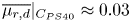 $\overline {\mu _{r,d}}|_{C_{PS40}} \approx 0.03$. Here, one can note that
  $\mu _{r,d} \lesssim \mu _r^{\phi _m^\infty }$ for each studied suspension.
Finally, the results of this study show that the globular/crushed PS particle geometry itself is enough to induce the rheological differences observed between  $C_{PS40}$ and
  $S_{PS40}$. To go further, it is quite satisfactory that
  $\mu _{r,d} \lesssim \mu _r^{\phi _m^\infty } \lesssim \mu _{r,s}$ for the two studied suspensions. We think that the experimental method described in the present paper to characterise the resistance to rolling motion induced by particle shape can be considered as another step to estimate the rolling friction coefficient for usage in DEM simulations, because it gives a framework for the value of
  $\mu _r$ for real suspensions made of non-spherical particles. We recall that, in agreement with the works of Agarwal et al. (Reference Agarwal, Tripathi, Tripathi, Kumar, Chakrabarty and Nag2021) and Tripathi et al. (Reference Tripathi, Kumar, Agarwal, Tripathi, Basu, Chakrabarty and Nag2021) in dry granular media, a more accurate estimation can be obtained by considering the particle eccentricity defined by
  $e/d$. However, two limits of this ratio exist: it cannot be considered for particles with a regular polygon shape (
 $e=0$) or a shape that deviates too much from a sphere. Therefore, the novelty of the present work is then to give a way of estimating a framework of
  $\mu _r$, particularly its upper (static) and lower (dynamic) bounds.
5. Concluding remarks
In this paper, two different but similar monodisperse suspensions have been sheared in a parallel plate rheometer in order to study their rheological behaviours and characterise their differences. More precisely, the main goal of the present paper was to study the influence of particle shape on the rheology of non-Brownian viscous frictional suspensions. Indeed, the rheology of suspensions composed of spherical particles has been studied extensively in the literature. However, understanding of the rheological behaviour of more complex suspensions composed of particles with irregular shape, which are more common in nature, remains more elusive. We have made two different suspensions composed of the same solid PS particles, separately dispersed in the same suspending Newtonian liquid. The only difference between the two lies in the shape of the particles present in each suspension: spheres in the first and crushed PS particles in the second.
We have then characterised the rheological behaviour of these different types of suspension by studying the variation of the jamming volume fraction with shear stress. Our main result shows that the suspension made of crushed particle is more viscous than the suspension made of spheres at small shear stress whereas the viscosity of the two suspensions becomes equivalent at large shear stress. This results in a stronger shear-thinning behaviour for the suspension made of crushed particles. This observation is notably reflected by a jamming volume fraction smaller at low shear stress for crushed particles whereas it is of the same order of magnitude as that for spheres when shear stress increases.
To go further, we have tried to understand the physical mechanism behind this observation, obviously induced by the different particle shapes. The literature pointed out the influence of rolling resistance but two different origins could be related to it and have been proposed: changes of adhesive force strength with particles’ local curvature and rolling resistance induced by locally normal contact forces acting at a non-spherical particle surface.
We have proposed two arguments which tend to demonstrate that adhesion is not important for the present rheological measurements. The first has been to show that the applied shear stress in the present study is much larger than the yield stress of suspensions (spheres and crushed). The second (and main) argument has been based on conducting shear reversal experiments and measuring the minimum value of viscosity,  $\eta _{min}$, and characteristic strains. The measurements of the same
  $\eta _{min}$ in the two types of suspensions and characteristic strains typical for non-adhesive particles was in contradiction with what could be expected if adhesive forces had played a significant role.
The second explanation relates the shear-thinning behaviour of both suspensions to a variable sliding friction,  $\mu _s$, whereas the larger viscosity at low shear stress for the non-spherical particles is assumed to be related to the particle shape. This physical origin for the shear-thinning behaviour is notably supported in the case of the PS spherical particles by the literature with the works of Lobry et al. (Reference Lobry, Lemaire, Blanc, Gallier and Peters2019) coupled with the AFM measurements on the same type of particles done by Arshad et al. (Reference Arshad, Maali, Claudet, Lobry, Peters and Lemaire2021) and Le et al. (Reference Le, Izzet, Ovarlez and Colin2023). Regarding the crushed particles, we have assumed a variation of
  $\mu _s$ with
  $\varSigma _{12}$ identical to the spherical particles, based on the fact that the crushed particles and the spherical particles are from the same material and of the same size. Moreover, the global aspect of the crushed particles does not deviate much from spheres. AFM measurements performed on the crushed particles could validate this assumption in the future.
The recent numerical work of Singh et al. (Reference Singh, Ness, Seto, de Pablo and Jaeger2020) has shown that the rolling resistance of solid particles plays a predominant role determining the jamming volume fraction,  $\phi _m$, when the sliding friction coefficient is large (
 $\mu _s \gtrsim 0.5$), but has almost no effect when
  $\mu _s$ is small. A quick comparison on the suspensions made of PS spheres and crushed particles in the frictionless case (PS particles in an aqueous solution) has shown no rheological differences, which is consistent with the absence of impact of
  $\mu _r$ when
  $\mu _s \rightarrow 0$. We have shown that it is possible to fit the variation of the jamming volume fraction with shear stress for both types of suspensions by the same variable sliding friction model (Lobry et al. Reference Lobry, Lemaire, Blanc, Gallier and Peters2019), simply by predicting a smaller value of the jamming volume fraction for crushed particles when the shear stress tends to zero (i.e. sliding friction coefficient grows ‘infinite’). The obtained value of
  $\phi _m^\infty$ (for which the predominant relative motion is rolling) from the fit (Lobry et al. Reference Lobry, Lemaire, Blanc, Gallier and Peters2019) coupled with the simulations of Singh et al. (Reference Singh, Ness, Seto, de Pablo and Jaeger2020) allowed us to obtain values of the apparent rolling friction coefficient for both types of suspension:
  $\mu _r^{\phi _m^\infty } = 0.03 \pm 0.02$ and
 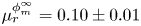 $\mu _r^{\phi _m^\infty } = 0.10 \pm 0.01$ for spheres and crushed particles, respectively.
The last part of the present paper has been focused on an experimental estimation of the rolling friction coefficient for both types of particles studied in the present paper. Faced with the difficulty of performing a direct experimental measurement for such small non-spherical particles, we decided to use an image analysis process consisting of approximating particles as irregular convex 2D polygons to measure the characterising shape parameters such as aspect ratio, internal angle and eccentricity, and finally calculate the values of the static rolling friction coefficient associated with each side of each polygon,  $\mu _r^{ij}$. The static rolling friction coefficient of each particle,
  $\mu _{r,s}$, has then been defined as the maximum value of all
  $\mu _{r,s}^{ij}$ characterising each particle. On the other hand, we have also determined the value of the dynamic friction coefficient,
  $\mu _{r,d}$, from the work needed to roll the particle over a distance equal to its own perimeter, analogous to Estrada et al. (Reference Estrada, Azéma, Radjai and Taboada2011). Therefore,
  $\mu _{r,d}$ can be then seen as an averaged value to characterise the shape-induced resistance of a particle to rolling motion based on the whole particle shape. In addition to the fact that the particle geometry of the two studied suspensions is enough to explain the rheological differences between the two, we have notably shown that the calculation of these two coefficient values (
 $\mu _{r,s}$ and
  $\mu _{r,d}$) gives a framework to estimate the value of
  $\mu _r$ for usage in numerical simulations.
Interestingly, a very good agreement with the recent works of Agarwal et al. (Reference Agarwal, Tripathi, Tripathi, Kumar, Chakrabarty and Nag2021) and Tripathi et al. (Reference Tripathi, Kumar, Agarwal, Tripathi, Basu, Chakrabarty and Nag2021) has been found and we confirmed that the eccentricity, defined as the ratio  $e/d$, gives a very good estimation of the value of rolling resistance for usage in DEM simulations, as long as the particle shape does not deviate too much from a sphere, and that
  $e \ne 0$.
To go further, the next step would be to find a way to directly measure the rolling friction coefficient of the particles (as is done by AFM measurements for  $\mu _s$), instead of deducing it by an image analysis process. Other difficulties encountered here concern the irregular shape of crushed particles, and the diversity of irregular shapes, which might invalidate the 2D approximation invoked here and make it harder to characterise the rolling resistance for irregular crushed particles. It is also true that different types of solid contact between the particles can exist in the crushed particles. In this paper, we have only considered a scenario where a particle rolls over a ‘mirror’ particle, but the physics is probably much more complex and it could be interesting to numerically study the distribution of the types of contact in such a suspension. Being aware of this, we think it could be interesting to compare the numerical results of Singh et al. (Reference Singh, Ness, Seto, de Pablo and Jaeger2020) with more regularly defined shapes such as cubic particles or other regular polygonal particles (for which
  $e=0$). Small hard fibres (
 $a_{ratio} \lesssim 2$) could also be an interesting shape. One can note that the angularity explored through the crushed particles in the present study remains close to spheres (
 $\alpha _j \rightarrow 180^\circ$). Studying cubes or rectangular shapes may then be interesting to explore smaller internal angles domains (
 $\alpha _j \rightarrow 90^\circ$). It would have the second advantage of increasing the value of
  $\mu _r$. Indeed, Singh et al. (Reference Singh, Ness, Seto, de Pablo and Jaeger2020) have shown that the influence of
  $\mu _r$ on
  $\phi _m$ is very large when
  $3 \times 10^{-2} \leqslant \mu _r \leqslant 3$. Cubes present this dual advantage of having a well-defined shape and an expected higher friction coefficient:
  $\mu _r$ is expected to be between 0.1 (dynamic) and 0.5 (static), for which Singh et al. (Reference Singh, Ness, Seto, de Pablo and Jaeger2020) have predicted a much lower jamming fraction,
  $0.44 \lesssim \phi _m^\infty \lesssim 0.53$. Thus, determining
  $\phi _m^\infty$ would show whether static or dynamic is more important. A rectangular shape (
 $a_{ratio} \lesssim 2$) offers two very different side lengths and allows one to study further the influence of the angular dependency of
  $\mu _r$.
Acknowledgements
We thank Y. Al-Majali and Y. Madraki for their assistance with crushing the particles, and we thank F. Peters and A. Singh for fruitful discussions. We acknowledge A. Singh for sharing his data from Singh et al. (Reference Singh, Ness, Seto, de Pablo and Jaeger2020).
Funding
This work was supported by the National Science Foundation (NSF; grant numbers CBET-1554044-CAREER and CBET-2210322).
Declaration of interests
The authors report no conflict of interest.
Appendix A. Process to crush the PS particles
Compression molding by a series of successive loading phases were done in order to crush the spherical PS particles. Figure 25 provides the schematics of the process. A dry sample of roughly  $2\unicode{x2013}4 \ {\rm ml}$ of PS beads were put between 2 steel plates, forming a layer about 10 particles thick and then compressed at room temperature by a load equivalent to approximately
  $80 \times 10^3 \ {\rm kg}$ (80 tonnes) for roughly 10 min. The particles were then observed under a microscope in order to check their shape. The process was then repeated if the shape of the particles was not satisfactory. Eventually, the loading operation on a given sample was repeated between 5 and 10 times. The particles were finally sieved to decrease the size distribution. Note that different processes of crushing were tried in order to get the non-spherical particles, notably by either increasing or decreasing the temperature or/and the load force. The process was tedious and very long but was determined to be the most appropriate in order to get the roughly 200 mg desired particle shape at the end.

Figure 25. Sketch of the compression process used to mold the PS particles shape: very long, tedious and meticulous work done by Yahya Al-Majali and Yasaman Madraki in order to get a few particles.
Appendix B. The image analysis process
The image processing is performed as follows. Each image taken with a microscope is binarised with a local threshold whose value  $T(x,y)$ is calculated individually for each pixel
  $(x,y)$. Here,
  $T(x,y)$ is a weighted sum (cross-correlation with a Gaussian window) of a
  $501 \times 501 \ {\rm px}^2$ neighbourhood of the pixel
  $(x,y)$ (see the OpenCV cv2.adaptiveThreshold website: https://docs.opencv.org/2.4/index.html). A rough delimitation of each particle in the picture is thus detected. However, the pixels belonging to the interior of a particle, whose grey level can be similar to the background, can be incorrectly identified as not being part of the particle. As a result, the interior of particles is ‘filled’ (see OpenCV cv2.floodFill) in order to correct it. The projected particles and their well-defined contours (red pixels in figure 20) are then detected through a watershed segmentation process (Vincent & Soille Reference Vincent and Soille1991, see OpenCV cv2.watershed). Finally, the contour of each particle is approximated as an irregular convex envelope (see OpenCV cv2.approxPolyDP, coloured in blue in figure 20) for which the (
 $x,y$) coordinates of each vertex
  $V_i$ (black dot except
  $G$ in figure 20) are known (
 $0 \leqslant i \leqslant n_s-1$, with
  $n_s$ the number of sides of the polygon).
Appendix C. Theoretical approach to determine the dynamic rolling friction coefficient
Let us consider that the centre of mass  $G$ travels left to right over a horizontal distance which is given by
  $\boldsymbol {x_G} = \delta x' + \delta x''$ (see figure 26). Under these conditions, the work required to displace the crushed particle over this given distance can be calculated as
 \begin{equation} W_p'|_j = \boldsymbol{F_N}\boldsymbol{\cdot}\boldsymbol{y_G} = F_N \times \delta y_j', \end{equation}
where  $\boldsymbol {y_G}$ is the vertical vector displacement of the centroid
  $G$ for which the force
  $F_N$ exerts a rolling resistance, and its norm is equal to
  $\delta y' = a_j - h_{ij}$. On the other hand, the work needed to displace a disc, characterised by a dynamic rolling friction coefficient
  $\mu _{r,d}$, over a distance equal to
  $\boldsymbol {x_G}$ is
 \begin{equation} W_d = \boldsymbol{F_T}\boldsymbol{\cdot}\boldsymbol{x_G} = 2\mu_{r,d}\, F_N \times \big(\delta x_j' + \delta x_j''\big). \end{equation}
Assuming equal work,  $W_p'|_j = W_d$, we arrive at the following mapping for the dynamic friction coefficient associated with the rotation from left to right around
  $V_j$:
 \begin{equation} \mu_{r,d}'|_j = \frac{1}{2}\left[\frac{\delta y'_j}{\delta x_j' + \delta x_j''}\right], \end{equation}
where  $\delta y_j' = a_j - h_{ij}$,
  $\delta x_j' = L_{ij}/2 + e_{ij}$ and
  $\delta x_j'' = L_{jk}/2 + e_{jk}$ (with
  $e_{ij}$ and
  $e_{jk}$ positive or negative). Note that, in the case for which the particle rolls around
  $V_j$ from the right to the left,
  $\mu _{r,d}$ is defined as
 \begin{equation} \mu_{r,d}''|_j = \frac{1}{2}\left[\frac{\delta y_j''}{\delta x_j' + \delta x_j''}\right], \end{equation}
where  $\delta y_j'' = a_j - h_{jk}$. Obviously, if the polygon is regular (
 $L_{ij} = L_{jk}$,
  $e_{ij} = e_{jk} = 0$,
  $h_{ij} = h_{jk}$), then
  $\mu _{r,d}=\mu _{r,d}'|_j=\mu _{r,d}''|_j$ and we arrive at the following mapping between
  $\mu _{r,d}$ and the dilatancy angle (
 $\psi = \psi '_j=\psi ''_j \ \forall\ j \in [0 \ n_s-1]$), already found by Estrada et al. (Reference Estrada, Azéma, Radjai and Taboada2011):
 \begin{equation} \mu_{r,d} = (1/4)\tan \psi \quad \text{with} \ \psi = \frac{\rm \pi}{2n_s}. \end{equation}
Figure 26. Sketch analogous to figure 22 of a partial crushed particle, considered as an irregular convex polygon with a centre of mass  $G$. Two sides of the polygon/crushed particle,
  $V_i V_j$ and
  $V_j V_k$, are outlined in dark blue. Tangential and normal forces,
  $\boldsymbol {F_T}$ and
  $\boldsymbol {F_N}$ (not represented here to avoid overloading the schema), respectively, are applied on the centre of mass
  $G$ of the particle as shown in figure 22 to create a rolling motion from left to right around
  $V_j$. Under these conditions,
  $V_i$ is the other vertex (with
  $V_j$) considered initially in direct contact with the mirrored particle, whereas
  $V_k$ is that which will be in contact at the end of the rotation around
  $V_j$. The initial (prime) location of each point is displayed with a black point and annotated (
 $'$), whereas the final (second) position is displayed with a transparent dot and annotated (
 $''$). Analogous to figure 22,
  $\alpha _j$ corresponds to the internal angle of the polygon/particle at
  $V_j$ (
 $\alpha _j = \widehat {V_i V_J V_k}$),
  $\theta _{ij}$ and
  $\theta _{jk}$ are the angles between the segments
  $h_{ij}$ and
  $GV_j$, and
  $h_{jk}$ and
  $GV_j$, respectively. Here
  $h_{ij}$ and
  $h_{jk}$ are the heights of
  $G$ from the segment
  $V_i V_j$ and
  $V_j V_k$, respectively. The eccentricity for the sides
  $V_i V_j$ and
  $V_j V_k$ corresponds to the lengths
  $|\boldsymbol {e_{ij}}|/d$ and
  $|\boldsymbol {e_{jk}}|/d$, respectively. The angle
  $\psi '$ (respectively,
  $\psi ''$) is the dilatancy angle when the particle rolls from the left to the right (respectively, from the right to the left) around
  $V_j$.
In our case, the polygons are irregular and, thus, the required work to roll around one vertex is not the same for all the vertices of a particle, as is shown qualitatively in figure 23 (the volume of each coloured peak is different). Unlike the static friction coefficient,  $\mu _{r,s}$, for which we have considered the maximum resistant torque to rolling motion, we define
  $\mu _{r,d}$ by considering the whole particle. The sum of the work for rolling over all vertices
  $W_p'|_j$ (or
  $W_p''|_j$) corresponds to the total work needed to displace a given particle over a distance equal to its perimeter
  $P_p$, and the value of the dynamic friction coefficient
  $\mu _{r,d}$ associated with the given particle can then be determined by the equation
 \begin{equation} \mu_{r,d} = \displaystyle\sum_{j=0}^{n_s-1} \mu_{r,d}'|_j = \frac{1}{2P_p}\displaystyle \sum_{j=0}^{n_s-1} \delta y'_j, \end{equation}
where:
(i)
$\delta y'_j = a_{j} - h_{ij}$ if $a_i < \sqrt {L_{ij}^2 + h_{ij}^2}$;(ii) else
$\delta y'_j = 0$.


 Open access