


1. Introduction
The widespread use of rotors in engineering systems such as propellers, rotorcraft and wind turbines has brought increasing attention to their noise generation. In particular, the interaction of a rotor with turbulent inflow is known to be a significant and often dominant source of noise in such systems. Realistic turbulent flows encountered by a rotor can arise from, for example, fuselage (hull) boundary layers of aircraft (marine vehicles) and wakes of upstream objects such as lifting or control surfaces and support structures. They are spatially inhomogeneous and contain a broad range of spatial and temporal scales, which can induce broadband as well as tonal rotor acoustic response. In order to facilitate the aeroacoustic design of rotors and develop noise-reduction technologies, accurate noise prediction and a clear understanding of the flow physics behind rotor-noise generation are required. The present study is aimed at advancing both the prediction of rotor turbulence-ingestion noise and knowledge of its source mechanisms through high-fidelity numerical simulations. Of special interest is the effect of coherent structures in the turbulent inflow on the spectral characteristics of the acoustic field.
Theoretical models of turbulence-ingestion noise have traditionally relied upon simplifying approximations, including the strip theory that treats a rotor blade as a series of airfoils along the blade span, a thin-airfoil gust-response theory (Sears Reference Sears1941; Amiet Reference Amiet1975; Roger & Moreau Reference Roger and Moreau2005) to estimate the unsteady aerodynamic loading on blade sections, and an aeroacoustic theory such as the Ffowcs Williams–Hawkings (FW-H) equation (Ffowcs Williams & Hawkings Reference Ffowcs Williams and Hawkings1969) to relate the unsteady loading to the radiated acoustic field. The model input representing the turbulent inflow is also highly idealised; it is typically based on empirical models of the wavenumber spectra and correlation length scales for homogeneous and isotropic turbulence (e.g. Mani Reference Mani1971; Homicz & George Reference Homicz and George1974). Over the years, improvements have been made to various aspects of gust-response models to include, for example, the effects of the airfoil thickness and shape (e.g. Gershfeld Reference Gershfeld2004; Moreau, Roger & Jurdic Reference Moreau, Roger and Jurdic2005) and inflow distortions due to the presence of the airfoil (e.g. Santana et al. Reference Santana, Christophe, Schram and Desmet2016; Zhong et al. Reference Zhong, Zhang, Peng and Huang2020). Models allowing more realistic turbulent inflow have also been developed (e.g. Catlett, Anderson & Stewart Reference Catlett, Anderson and Stewart2012; Glegg, Devenport & Alexander Reference Glegg, Devenport and Alexander2015). Catlett et al. (Reference Catlett, Anderson and Stewart2012) proposed a velocity-correlation model for the turbulent inflow that incorporates the effect of inhomogeneity and anisotropy through a coordinate transformation. Using this model in the Sears theory and treating the rotor as an acoustically compact dipole source, they obtained an improved prediction of the noise from a rotor behind the trailing edge of an airfoil relative to the prediction of an isotropic inflow model. Glegg et al. (Reference Glegg, Devenport and Alexander2015) developed a time-domain theory to facilitate rotor-noise prediction using inflow data measured experimentally in terms of the space–time correlations of the upwash velocity, and obtained reasonable noise predictions compared with the experimental measurements for a rotor partially immersed in a planar turbulent boundary layer (TBL) at low and moderate thrust. Despite the theoretical advances, turbulence-ingestion noise models still do not capture the full three-dimensional effect of the rotor geometry, the aerodynamic interaction among blades and the complex turbulent inflow in real-world applications.
With the advancement in high-performance computing capabilities and numerical algorithms, high-fidelity, scale-resolving simulations have emerged as an effective tool for the prediction and investigation of turbulence-ingestion noise and, more generally, turbomachinery noise. Several simulation techniques have been employed, including large-eddy simulation (LES) (e.g. Carolus, Schneider & Reese Reference Carolus, Schneider and Reese2007; Wang, Wang & Wang Reference Wang, Wang and Wang2015, Reference Wang, Wang and Wang2021; Wu et al. Reference Wu, Yangzhou, Ma and Huang2023), hybrid methods combining Reynolds-averaged Navier–Stokes simulation with LES (e.g. Suzuki et al. Reference Suzuki, Spalart, Shur, Strelets and Travin2018, Reference Suzuki, Spalart, Shur, Strelets and Travin2019; Arroyo et al. Reference Arroyo, Leonard, Sanjose, Moreau and Duchaine2019), and the lattice-Boltzmann method (e.g. Casalino, Hazir & Mann Reference Casalino, Hazir and Mann2018; Moreau Reference Moreau2019a). A review of the current state-of-the-art of turbomachinery noise modelling and computation has been provided by Moreau (Reference Moreau2019b). Among those researchers conducting studies most relevant to the present work, Carolus et al. (Reference Carolus, Schneider and Reese2007) were perhaps the first to apply LES to an entire rotor for predicting turbulence-ingestion noise. They considered a ducted fan with six blades downstream of a turbulence-generating grid in a low-Mach-number flow. Using an incompressible, finite-element computation with only five million elements and a noise model for ducted turbomachinery, they were able to obtain favourable comparisons with measurements at certain frequencies. Wang et al. (Reference Wang, Wang and Wang2015, Reference Wang, Wang and Wang2021) and Wang, Wang & Wang (Reference Wang, Wang and Wang2017) conducted systematic studies of rotor turbulence-ingestion noise in low-Mach-number flows using incompressible-flow LES and the FW-H equation. They first considered a 10-bladed Sevik rotor (Sevik Reference Sevik1974) ingesting grid-generated turbulence (Wang et al. Reference Wang, Wang and Wang2015; Wang Reference Wang2017) as in the experiment of Wojno, Muller & Blake (Reference Wojno, Muller and Blake2002a,Reference Wojno, Muller and Blakeb) and achieved overall agreement with the measurements in terms of the sound pressure spectral shape and level. The turbulence-ingestion noise was found to be broadband with small peaks at the blade-passing frequency (BPF) and its harmonics, and significantly stronger than the rotor self-noise generated by blade trailing-edge vortex shedding. Rotor ingestion of grid turbulence was also studied recently by Wu et al. (Reference Wu, Yangzhou, Ma and Huang2023), who conducted LES of the Sevik (Reference Sevik1974) experiment involving the Sevik rotor behind a turbulence grid. Two grids of different spacings and bar diameters were considered, and the computed rotor unsteady-thrust spectra were shown to predict the experimental results better in terms of both the broadband content and the spectral hump at the BPF than the theoretical model. The acoustic field emitted by the rotor was also calculated.
In a subsequent study, Wang et al. (Reference Wang, Wang and Wang2017, Reference Wang, Wang and Wang2021) investigated the aeroacoustics of a modified Sevik rotor ingesting the turbulent wake of a circular cylinder as in an experiment conducted at Virginia Tech (VT) (Alexander et al. Reference Alexander, Molinaro, Hickling, Murray, Devenport and Glegg2016; Hickling et al. Reference Hickling, Alexander, Molinaro, Devenport and Glegg2017; Molinaro et al. Reference Molinaro, Balantrapu, Hickling, Alexander, Devenport and Glegg2017). The computed sound pressure spectra showed excellent agreement with measurements, capturing all important spectral features including the broadband content, a strong peak induced by the strikes of coherent vortices shed from the cylinder, a second peak at the rotor BPF and a minor peak associated with vortex shedding from the blade trailing edge. The effects of the rotor advance ratio and the radial position at which the wake strikes the rotor were also captured correctly (Wang Reference Wang2017; Wang et al. Reference Wang, Wang and Wang2017, Reference Wang, Wang and Wang2021). The detailed LES data were used to analyse the blade dipole-source distribution and correlations along with the space–time characteristics of the upwash-velocity field encountered by the rotor. Their results demonstrated that the Sears theory was able to provide a reasonable prediction of the rotor noise at the important mid-frequencies, based on which a mixed scaling for sound pressure spectra using the free-stream and convection Mach numbers was proposed and validated.
An important feature frequently observed in turbulence-ingestion noise is the spectral humps near multiples of the BPF. These humps, known as ‘haystacks’ or ‘haystacking’ in the literature, are generally regarded as being caused by successive blades cutting through the same coherent flow structures and, as a result, correlated dipole radiation (Murray et al. Reference Murray, Devenport, Alexander, Glegg and Wisda2018; Huang Reference Huang2023). However, an in-depth knowledge of blade interaction with the turbulence structure and the spectral-hump formation is still lacking, which is one of the motivations of the present study. Spectral humps were observed in the grid-turbulence experiment of Sevik (Reference Sevik1974), but his theoretical prediction based on a thin-airfoil theory and an isotropic-turbulence correlation model failed to capture the humps because it did not account for blade-to-blade correlations. Streamtube contraction induced by a rotor can elongate the vortical structures as they are drawn towards the rotor and thereby strengthen blade-to-blade correlations. This was investigated theoretically by Majumdar & Peake (Reference Majumdar and Peake1998), who considered the noise produced by the ingestion of atmospheric turbulence by an aircraft-engine fan. Using rapid distortion theory along with the strip theory and asymptotic techniques, their analysis showed that under static test conditions high distortions of incoming turbulence lead to strong spectral peaks, whereas under typical flight conditions the eddies are much less distorted and the noise is generally broadband. This is consistent with the earlier experimental results of Hanson (Reference Hanson1974). Robison & Peake (Reference Robison and Peake2014) extended the analysis of Majumdar & Peake (Reference Majumdar and Peake1998) to turbulent inflows that are non-axisymmetric and reached the same qualitative conclusion. Huang (Reference Huang2023) recently provided an alternative interpretation of the haystacking phenomenon in terms of the convolution of an inhomogeneous gust and a periodic sampling function representing blade cutting. The convolution model was shown to be able to describe the frequency shift of the ingested gust to around the BPF and its harmonics and account for the effect of the rotor thrust (advance ratio). New experimental insights have been generated through a series of aeroacoustic measurements at VT. Alexander, Devenport & Glegg (Reference Alexander, Devenport and Glegg2017) and Murray et al. (Reference Murray, Devenport, Alexander, Glegg and Wisda2018) measured the noise from a 10-bladed, modified and scaled-up Sevik rotor partially immersed in a thick, planar TBL. They observed haystacking spectral peaks at the BPF and its first few harmonics, whose magnitudes grew with increasing thrust. At high thrust, the haystacks were found to become markedly narrower and appear at more BPF harmonics, which was attributed to boundary-layer separation from the wall in the vicinity of the rotor blade disc and blade interaction with the vortex structures in the separation region. The same modified Sevik rotor was used by Alexander et al. (Reference Alexander, Molinaro, Hickling, Murray, Devenport and Glegg2016) and Molinaro et al. (Reference Molinaro, Balantrapu, Hickling, Alexander, Devenport and Glegg2017) to study the turbulence ingestion of the wake of a circular cylinder at various thrusting conditions. Haystacking peaks were observed at high-thrust conditions but they were broader and fewer than in the case of planar boundary-layer ingestion. At zero and low thrusts, only the BPF peak was clearly discernible as in the numerical results of Wang et al. (Reference Wang, Wang and Wang2021).
More recently, Hickling et al. (Reference Hickling, Balantrapu, Millican, Alexander, Devenport and Glegg2019) and Hickling (Reference Hickling2020) experimentally investigated the sound from a five-bladed rotor ingesting a thick TBL at the downstream end of a body of revolution (BOR) at zero angle of attack. The BOR, whose exact geometry is described in § 2.1, has an ellipsoidal nose, a cylindrical centrebody of 0.432 m in diameter and a  $20^\circ$ tail cone. The length-to-diameter ratio of the BOR is $3.17$. The free-stream velocity is $U_\infty = 20.3$ m s $^{-1}$, which corresponds to a free-stream Mach number of $0.059$ and length-based Reynolds number of $1.9 \times 10^6$. The rotor is completely immersed in the TBL at the end of the tail cone. Radiated sound was measured with a microphone array at rotor advance ratios corresponding to zero-thrust and moderately thrusting conditions. The integrated spectra from the measured beamforming map showed broadband noise and haystacking peaks at frequencies close to but right-shifted (i.e. shifted up) by $7$–
$7$– $12\,\%$ from the BPF and its harmonics. From the spectral ‘haystacks’ it was inferred that the rotor inflow contained turbulence structures sufficiently long to allow multiple cutting by rotor blades as they are convected through the rotor. Hot-wire and particle image velocimetry (PIV) velocity measurements were made in the tail-cone boundary layer with and without the rotor present (Hickling et al. Reference Hickling, Balantrapu, Millican, Alexander, Devenport and Glegg2019; Balantrapu et al. Reference Balantrapu, Hickling, Alexander and Devenport2021) to characterise the turbulent inflow to the rotor. In the case of flow over the same BOR without a rotor, extensive analysis was performed by Balantrapu et al. (Reference Balantrapu, Hickling, Alexander and Devenport2021) to examine the velocity statistics and structure in the boundary layer under the influences of adverse pressure gradient and surface curvature. They found that the mean-velocity and turbulence-intensity profiles are self-similar with the embedded-shear-layer scaling of Schatzman & Thomas (Reference Schatzman and Thomas2017). Two-point correlations of the streamwise velocity as a function of axial and radial separations were obtained at the tail-cone end, which is considered the rotor inflow plane, from PIV measurements. From comparisons with the two-point correlations estimated based on single-point hot-wire measurements and Taylor's hypothesis, they estimated the convection velocity and noted that it is significantly higher than the local mean velocity. Wall-pressure fluctuations underneath the tail-cone boundary layer were also measured and analysed (Balantrapu, Alexander & Devenport Reference Balantrapu, Alexander and Devenport2023).
In the present study, carried out in parallel with the aforementioned VT experiment (Hickling et al. Reference Hickling, Balantrapu, Millican, Alexander, Devenport and Glegg2019; Hickling Reference Hickling2020; Balantrapu et al. Reference Balantrapu, Hickling, Alexander and Devenport2021), the aeroacoustics of rotor interaction with the BOR boundary layer is analysed computationally. A well-resolved numerical simulation provides unimpeded access to flow-field details in space and time, thereby allowing analyses leading to deep insight into the acoustic source mechanisms, particularly with regard to the role of turbulence structures in the TBL. The computational approach is based on a combination of LES with the FW-H equation as in Wang et al. (Reference Wang, Wang and Wang2021). However, the TBL inflow to the rotor is significantly more challenging to compute than the cylinder-wake inflow in the case of Wang et al. (Reference Wang, Wang and Wang2021) because of the large surface area of the BOR and wider range of turbulence scales, and thus an evaluation of the LES predictive capability for rotor noise in wall-bounded flows is an additional objective of the study.
To accurately predict the rotor noise, the turbulence structures and their evolution in the tail-cone boundary layer must be computed accurately. The accuracy was verified by first computing flow over the BOR without a rotor (Zhou, Wang & Wang Reference Zhou, Wang and Wang2020) and comparing the results with the VT experimental data (Hickling et al. Reference Hickling, Balantrapu, Millican, Alexander, Devenport and Glegg2019; Balantrapu et al. Reference Balantrapu, Hickling, Alexander and Devenport2021, Reference Balantrapu, Alexander and Devenport2023). Reasonable agreement was obtained in terms of velocity and turbulence-intensity profiles, energy spectra and frequency spectra of surface-pressure fluctuations. Computational expenses were reduced by employing a wall model in the nose and centrebody sections of the BOR while keeping the acoustically important tail-cone section wall-resolved. This partially wall-modelled approach was shown to be as accurate in the tail-cone region as wall-resolved LES and thus suitable for rotor-noise computation (Zhou et al. Reference Zhou, Wang and Wang2020). The same approach was used by Posa & Balaras (Reference Posa and Balaras2020) with an immersed-boundary method in their study of the flow around a DARPA SUBOFF body, which is an axisymmetric BOR with appendages, at a length-based Reynolds number of  $1.2\times 10^7$. The simulation results were in good agreement with published experimental data and used to investigate the effect of the Reynolds number by comparison with their previous wall-resolved LES results at a lower Reynolds number of $1.2\times 10^6$ (Posa & Balaras Reference Posa and Balaras2016). The SUBOFF geometry is a widely studied BOR with extensive experimental data available for validating computational approaches. Other high-fidelity simulations with this configuration include the wall-resolved LES of Kumar & Mahesh (Reference Kumar and Mahesh2018) for flow around a SUBOFF hull without stern appendages at a reduced Reynolds number of $1.1 \times 10^6$ and the earlier computations of Alin et al. (Reference Alin, Bensow, Fureby, Huuva and Svennberg2010) for the SUBOFF hull, both with and without appendages, at the experimental Reynolds number of $1.2\times 10^7$ to evaluate the feasibility of wall-modelled LES and detached-eddy simulation for submarine flows.
As will be demonstrated in this paper, the LES with zonal wall-modelling approach adopted in the present study is capable of providing accurate statistical descriptions and structures of the tail-cone boundary layer of the BOR, and thereby satisfactory turbulent inflow for rotor turbulence-ingestion noise calculation. Using the unsteady blade loading obtained from the LES, the FW-H prediction captures both the broadband and the haystacking acoustic responses of the rotor to the inflow turbulence. A major contribution of this work is the elucidation of the haystacking mechanism through a detailed analysis of the blade dipole sources in relation to the coherent structures encountered by the rotor in the decelerating TBL. The analysis shows that multiblade interaction with the same coherent structure produces not only modulating peaks but also valleys in the broadband sound pressure spectra as a result of constructive and destructive interference among correlated dipole radiation. Consequently, it is suggested that the commonly used term ‘haystacking’ is not an accurate description of this phenomenon, as it acknowledges only the spectral peaks superimposed on the baseline broadband level.
The rest of the paper is organised as follows. Section 2 describes the computation and validation of the BOR boundary layer and its interaction with the rotor, and gives an overview of the flow-field characteristics and structure. Section 3 discusses the computation, validation and scaling of the rotor noise arising from ingestion of the TBL. A detailed acoustic-source analysis is presented in § 4, which includes dipole source distributions on rotor blades, blade-to-blade correlations and coherence of the sectional dipole sources, and their relation to inflow turbulence structures. Through the correlation analysis and a comparison of the noise produced by a single blade and by the entire rotor, the origin of the modulating peaks and valleys of the sound pressure spectra is unambiguously identified. Finally, the major findings of this work are summarised in § 5.
2. Tail-cone boundary layer and rotor interaction
2.1. Configuration
The flow configuration and computational domain are shown schematically in figure 1. The BOR consists of a cylindrical midsection of diameter  $D$ and equal length, a 2 : 1 ellipsoidal nose of length $D$, and a tail cone with a $20^\circ$ half-apex angle that is connected to a thin cylindrical support pole of diameter $0.148D$. The tail-cone angle was selected to achieve the thickest possible boundary layer at the tail end without separation. A circumferential trip ring with a $(0.0019D)^2$ cross-section is positioned at the end of the nose to induce transition to turbulence in the experiment. In the numerical simulation the trip-ring height was halved, which was found to produce a better match with the experimental boundary-layer thickness in the fully turbulent region downstream. The BOR is at zero angle of attack and the experimental Reynolds number of $Re_L=U_\infty L/\nu =1.9\times 10^6$ based on the free-stream velocity and the BOR length, $L=3.17D$. The free-stream Mach number is $M_\infty = 0.059$. Both cylindrical coordinates ( $x$,
$x$,  $r$,
$r$,  $\theta$) and Cartesian coordinates ( $x$,
$x$,  $y$,
$y$,  $z$) are used in the present study, with the coordinate origin fixed at the centre of the cross-section at the nose end and the $z$- and $\theta$-coordinates obeying the right-hand rule.

Figure 1. Flow configuration and simulation set-up.
A five-bladed rotor is positioned behind the BOR with its centreplane  $0.08D$ downstream of the tail-cone end. The rotor geometry can be found in the inset of figure 1 (see also figure 3). It has a tip diameter of $D_r=0.5D$ and a hub diameter of $0.296D_r$, which matches the diameter of the support pole. The blade height is similar to the boundary-layer thickness at the end of the tail cone, allowing the rotor to be fully immersed in the boundary layer. At $75\,\%$ radius, the blades attain a maximum chord of $0.264D_r$, maximum thickness of $0.0278D_r$, and blade pitch of $0.778D_r$. Blade sections have a rounded trailing edge of $8.33 \times 10^{-4}D_r$ radius, and the maximum sectional skew angle is $35.5^\circ$ near the tip. The Reynolds number based on the free-stream velocity and the maximum chord length, $Re_C=U_\infty C_{{max}}/\nu$, is $7.9 \times 10^4$. Two rotor advance ratios, $J=U_\infty /(n D_r)=1.44$ and $1.13$ where $n$ is the rotational speed in revolutions per second, are considered in the present study. These two cases are selected based on the availability and quality of the VT experimental data (Hickling et al. Reference Hickling, Balantrapu, Millican, Alexander, Devenport and Glegg2019; Hickling Reference Hickling2020).
2.2. Simulation method
Flow simulations are based on the spatially filtered, incompressible Navier–Stokes equations and the continuity equation in the rotor frame of reference using a conservative, absolute velocity formulation (Beddhu, Taylor & Whitfield Reference Beddhu, Taylor and Whitfield1996). A finite-volume, unstructured-mesh LES code developed at Stanford University (You, Ham & Moin Reference You, Ham and Moin2008) is enhanced with the rotating-frame formulation and a wall model to carry out the simulations. The cell-based numerical scheme employs energy-conservative, low-dissipative spatial discretisation and a fully implicit fractional-step method for time advancement. It is second-order accurate in both space and time. The Poisson equation for pressure is solved using the Generalized Product Bi-Conjugate Gradient with Safety convergence (GPBiCGSafe) method of Fujino & Sekimoto (Reference Fujino and Sekimoto2012). The subgrid-scale stress is modelled using the dynamic Smagorinsky model (Germano et al. Reference Germano, Piomelli, Moin and Cabot1991). The accuracy of this code for aeroacoustic calculations has been established in a number of configurations including rough-wall boundary layers (Yang & Wang Reference Yang and Wang2013), tandem cylinders (Eltaweel et al. Reference Eltaweel, Wang, Kim, Thomas and Kozlov2014) and, more pertinent to the present work, a rotor ingesting a turbulent wake (Wang et al. Reference Wang, Wang and Wang2021).
To reduce the computational cost associated with the large surface area of the BOR and the high Reynolds number, LES is combined with a wall model in the nose and midsection regions of the BOR. The tail-cone region is critically important for the development of the TBL that feeds turbulent inflow into the rotor, and is therefore wall-resolved. The equilibrium stress-balance model (Cabot & Moin Reference Cabot and Moin2000; Piomelli & Balaras Reference Piomelli and Balaras2002; Wang & Moin Reference Wang and Moin2002) is employed in the wall-modelled LES to provide approximate wall shear-stress boundary conditions to the LES. The efficacy and accuracy of this zonal wall-modelling approach have been established in a previous study of the BOR boundary layer without the rotor (Zhou et al. Reference Zhou, Wang and Wang2020).
The cylindrical computational domain is of length  $11.17D$ and radius $2.39D$ as illustrated in figure 1. The radius of the domain is chosen to provide the same blockage ratio as in the VT wind tunnel. The boundary conditions consist of a uniform inflow at the inlet, stress-free conditions with radial velocity $u_r=0$ on the outer boundary, no-slip and no-penetration conditions for wall-resolved LES and approximate wall shear stress for wall-modelled LES on solid surfaces, and convective outflow conditions at the exit.
Hybrid meshes are employed in the simulations. Structured-mesh blocks are used around the entire BOR, rotor blades, rotor hub and support pole, and unstructured mesh is employed elsewhere. Around the nose and the centrebody where a wall model is used, the meshes are relatively coarse. In the middle of the centrebody, the grid spacings in wall units estimated based on the wall shear stress from the wall model are  ${\rm \Delta} x^+ \approx 130$ in the streamwise direction, $(R{\rm \Delta} \theta )^+ \approx 61$ in the azimuthal direction and ${\rm \Delta} r_{{min}}^+ \approx 24$ in the wall-normal direction. The grid around the wall-resolved tail-cone section is finer, consisting of 1200 streamwise cells and 1600 azimuthal cells, both uniformly spaced, and 130 cells across the thickness of the boundary layer at the end of the tail cone. The wall-normal spacing ${\rm \Delta} r_{{min}}^+$ for the first off-wall cells within the tail-cone section is less than 2, and transition from the coarser midsection mesh to the finer tail-cone mesh is gradual. Grid-converged statistics for flow over the BOR have been demonstrated in the previous simulations without the rotor (Zhou et al. Reference Zhou, Wang and Wang2020). Compared with the two meshes used in that case, the present mesh in the tail-cone section has the same number of streamwise cells as the fine mesh, and the numbers of azimuthal and radial cells are between the fine and coarse meshes, thus ensuring grid convergence.
Surrounding the rotor is a cylindrical mesh block  $0.12D_r$ long and $1.05D_r$ in diameter, located between $x/D=2.22$ and $2.28$, which are $0.01D_r$ upstream of the rotor-blade leading edge and $0.02D_r$ downstream of the rotor-blade trailing edge, respectively. As in Wang et al. (Reference Wang, Wang and Wang2021), the grid is designed to capture the turbulence-ingestion noise but insufficient to resolve the blade boundary layers and thereby the rotor self-noise accurately. Two meshes of different resolutions are employed to check grid convergence. On the coarse mesh, the blade surface on each side contains $100$ cells in the chordwise direction and $190$ cells in the radial direction, with grid spacings not exceeding $0.0034D_r$ and $0.002D_r$, respectively. The wall-normal spacing for the first off-wall cells is within $0.0006D_r$. On the fine mesh there are $200$ and $380$ surface cells in the chordwise and radial directions, respectively, on each side of the blade, and the corresponding grid spacings are no larger than $0.002D_r$ and $0.0011D_r$. The largest wall-normal spacing for the first off-wall cells is $0.0003D_r$. In both cases the resolution within the rotor block is at least comparable to, and generally better than, that of the upstream tail-cone TBL, and the grid is more refined around the rotor blades and within the blade passages. For convenience the meshes with coarser and finer rotor blocks are henceforth simply referred to as coarse mesh and fine mesh, respectively, even though they share the same mesh outside the rotor block. The coarse mesh contains approximately $5 \times 10^7$ cells in the rotor block and $5.5 \times 10^8$ cells in total, and the fine mesh contains approximately $1.2 \times 10^8$ cells in the rotor block and $6.2 \times 10^8$ cells in total.
The time step sizes in all simulations are determined based on a maximum Courant–Friedrichs–Lewy number of  $1.2$. The mean time steps in the fine-mesh simulations are $2.4 \times 10^{-5}D/U_\infty$ for the case of $J=1.44$ and $2.0 \times 10^{-5}D/U_\infty$ for $J=1.13$, corresponding to approximately $0.012^\circ$ and $0.013^\circ$ of blade rotation per step, respectively. The simulations are first run for over one flow-through time ( $11.17D/U_\infty$) to wash out initial transients, and then run for approximately another flow-through time, or more precisely 16 and 20 rotor rotations for $J=1.44$ and $1.13$, respectively, to collect data for statistical analysis. Statistical convergence is verified through a comparison with results based on one-half of the sampling period.
2.3. Flow field and validation
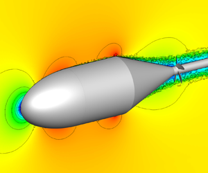
In this section, the simulation results for the flow field around the BOR and the rotor are presented. All results are from the fine-mesh simulation unless indicated otherwise. Figure 2(a) shows isocontours of the instantaneous axial velocity for the  $J=1.44$ case in the $x$–
$x$– $y$ plane through the BOR axis. The flow accelerates around the nose and as it approaches the tail-cone upper corner, and decelerates in the tail-cone region under a strong adverse pressure gradient as the boundary layer thickens rapidly. The rotor does not have a significant effect on the downstream development of the boundary layer because it is lightly loaded. Figure 2(b,c) provides a close-up view of the instantaneous axial velocity field around the rotor from two different perspectives. It clearly illustrates the interaction of turbulence structures in the incoming boundary layer with the rotor blades, which is the source of blade unsteady loading and acoustic radiation. The instantaneous flow fields for the $J=1.13$ case have similar characteristics.

Figure 2. Instantaneous axial velocity  $u_x/U_\infty$ in (a) the $z=0$ plane; (b) the $z=0$ plane around the rotor; (c) the $x/D=2.25$ plane. The rotor advance ratio is $J=1.44$.
Figure 3 shows the instantaneous radial vorticity on two cylindrical surfaces at  $r/D=0.13$ and $0.21$, also for the $J=1.44$ case. Turbulence structures in the incoming boundary layer are seen to convect downstream through the blade passages and interact with rotor blades, causing large fluctuations in blade loading. Because of the relatively low chord Reynolds number, the boundary layers around the blades are not fully turbulent and no clear vortex shedding from the trailing edge is observed, although the wake is quite unsteady.

Figure 3. Instantaneous radial vorticity,  $\omega _r D/U_\infty$, on two cylindrical surfaces for $J=1.44$: (a) $r/D=0.13$; (b) $r/D=0.21$.
Figure 4 depicts isocontours of the phase-averaged axial velocity at three different streamwise locations  $x/D=2.17$, $2.25$ and $2.27$, corresponding to the end of the tail cone, the rotor midplane and immediately downstream of the blade trailing edge, respectively, for both rotor advance ratios. The phase averaging is calculated by averaging in time in the rotor frame of reference. The wake of the BOR is notably thinner in the $J=1.13$ case, particularly in the midplane and trailing-edge plane, because the faster rotational speed allows faster flow through the rotor. The effect of tip vortices is clearly visible in the $J=1.13$ case. In figure 5, the phase-averaged turbulent kinetic energy (TKE) is shown at the same three streamwise locations. It can be noted that the rotor advance ratio only slightly influences the TKE except in the blade wake, where the rotor produces stronger TKE in a larger wake region near the blade tip as the advance ratio is reduced.

Figure 4. Phase-averaged axial velocity,  $U_x/U_{\infty }$, for (a–c) $J=1.44$ and (d–f) $J=1.13$ at three streamwise locations: (a,d) $x/D=2.17$; (b,e) $x/D=2.25$; (c,f) $x/D=2.27$.

Figure 5. Phase-averaged TKE,  $\overline {u_i^{\prime }u_i^{\prime }}/(2U_{\infty }^2)$, for (a–c) $J=1.44$ and (d–f) $J=1.13$ at three streamwise locations : (a,d) $x/D=2.17$; (b,e) $x/D=2.25$; (c,f) $x/D=2.27$.
A quantitative validation of the rotor inflow obtained from LES is shown in figures 6 and 7 in comparison with the PIV measurements at VT (Hickling et al. Reference Hickling, Balantrapu, Millican, Alexander, Devenport and Glegg2019; Hickling Reference Hickling2020). In figure 6, profiles of the mean axial velocity and the root mean square (r.m.s.) of the axial and azimuthal velocity fluctuations along the radial direction in the stationary frame of reference are plotted at the tail-cone end of the BOR,  $x/D=2.17$, which is $0.055D$ upstream of the rotor leading edge and henceforth considered the rotor inflow plane. The agreement between the LES and experimental data is reasonable for both rotor advance ratios. The thicknesses of the boundary layers are somewhat overpredicted as suggested by the mean velocity profiles. Although there are small discrepancies in velocity fluctuations, the overall distributions and locations of peak fluctuations agree well with the experiment.

Figure 6. Profiles of (a,d) mean axial velocity and r.m.s. of (b,e) axial and (c,f) azimuthal velocity fluctuations at  $x/D = 2.17$ as a function of the radial coordinate in the stationary frame of reference, compared with experimental data (Hickling Reference Hickling2020) for (a–c) $J=1.44$ and (d–f) $J=1.13$: solid red, LES; dash–dotted black, experiment.

Figure 7. Frequency spectra of axial velocity fluctuations for  $J=1.44$ compared with experimental data (Hickling Reference Hickling2020) at $x/D = 2.17$ and $r/D = 0.18$: solid red, LES; dash–dotted black, experiment; dashed black, line with $- 5/3$ slope.
Figure 7 shows the frequency spectra of axial velocity fluctuations at a radial position at the tail-cone end,  $x/D=2.17$ and $r/D=0.18$, for $J=1.44$. The computed spectrum compares reasonably well with the experimental data (Hickling Reference Hickling2020) for nearly two decades of frequencies. The spectral peak at $fD/U_\infty \approx 7$, which corresponds to the BPF, is captured very well. The high-frequency content of the spectrum is limited by the grid resolution of convecting turbulent eddies. Estimated based on the local axial grid spacing ${\rm \Delta} x/D \approx 0.0015$, mean axial velocity of approximately $0.5U_{\infty }$ and Taylor's hypothesis of frozen-eddy convection, the cutoff frequency is $f_c D/U_{\infty } \approx 167$ with spectral resolution. The wavenumber (frequency) resolution of the finite-volume scheme employed in this study is significantly lower, leading to an earlier falloff starting at $f D/U_\infty \approx 50$. Overall, the comparisons in figures 6 and 7 provide confidence that the spatial and temporal accuracy of the rotor inflow is adequate for acoustic analysis.
Figure 8 illustrates the evolution of turbulence structures in the tail-cone boundary layer for  $J=1.44$ in terms of the two-point correlations of the fluctuating axial velocity in a centreplane through the BOR axis for seven anchor positions. These anchor points are along a mean streamline that passes through $(x/D, r/D) = (2.17, 0.18)$, which is in the vicinity of peak turbulence intensity in the rotor inflow plane. Contour levels lower than $0.1$, including negative values, are not plotted to avoid overlap of patterns for different anchor locations. It can be seen that the spatial scales of flow structures increase rapidly in the downstream direction with growing boundary-layer thickness. Their evolution is virtually unaffected by the rotor except in its immediate vicinity, and the corresponding correlations in the $J=1.13$ case (not shown) are virtually the same except at the last station, where the effect of the rotor becomes noticeable. The two-point correlations of the fluctuating pressure on the tail-cone surface exhibit even more drastic increases in length scales in the downstream direction (Zhou et al. Reference Zhou, Wang and Wang2020). The growth of turbulence structures to sizes that allow interaction with successive blades is key to the generation of the haystacking acoustic peaks, as demonstrated in §§ 4.3 and 4.4.

Figure 8. Two-point correlations of axial velocity fluctuations for  $J=1.44$ at seven locations along a mean streamline in the tail-cone boundary layer.
2.4. Blade surface pressure
At the advance ratios  $J=1.44$ and $1.13$, the dimensionless thrust of the rotor obtained from the LES is $F_T/(\rho _\infty U_\infty ^2) = -1.18 \times 10^{-2}$ and $4.74 \times 10^{-4}$, respectively. These values indicate that the rotor is in reality operating under a slightly braking condition when $J=1.44$ and under a nearly zero-thrust condition when $J=1.13$. Figures 9 and 10 show distributions of the mean pressure and the r.m.s. of pressure fluctuations on the rotor blade surface. The results are obtained by averaging over time and all five blades, which are statistically equivalent, and the reference pressure is taken at the inlet of the computational domain near the outer boundary. For convenience the terms ‘pressure side’ and ‘suction side’ used here are with reference to the normal positive-thrust operating condition and not necessarily reflective of the actual loading. From figure 9, it can be noted that, overall, the mean pressure decreases from the blade root to the tip on both sides, and this decrease is more significant at the lower rotor advance ratio owing to the faster blade speed relative to the flow. Figure 10 shows that the pressure fluctuations are stronger in the blade leading-edge, trailing-edge and tip regions. The strong fluctuations at the leading edge are generated by its interaction with the incoming turbulent flow. In the blade-tip region, the tip vortex is responsible for the large pressure fluctuations. Figure 10 also shows that the level of blade-surface pressure fluctuations grows significantly with reduction of the advance ratio, again due to the faster blade speed.

Figure 9. Mean pressure,  $P/(\rho _\infty U_\infty ^2)$, on the rotor blade surface at (a,b) $J=1.44$ and (c,d) $J=1.13$: (a,c) suction side; (b,d) pressure side.

Figure 10. R.m.s. of pressure fluctuations,  $p'_{{rms}}/(\rho _\infty U_\infty ^2)$, on the rotor blade surface at (a,b) $J=1.44$ and (c,d) $J=1.13$: (a,c) suction side; (b,d) pressure side.
Figure 11 shows the chordwise distributions of the mean surface pressure and the r.m.s. of surface pressure fluctuations for the  $J=1.44$ rotor at $r/D=0.18$, which corresponds to the maximum chord length. To evaluate grid convergence, results from both the coarse- and fine-mesh LES are compared. It can be seen that the mean pressure curves from the different meshes agree well. The mean pressure is very high at the blade leading edge and decreases rapidly away from the leading edge. Further downstream, the mean pressure gradually increases towards the trailing edge. In terms of the r.m.s. values of the fluctuating pressure, the fine-mesh result agrees well with the coarse-mesh result over a large portion of the blade chord, but some notable differences occur near the trailing edge. Fortunately, the differences are relatively small and do not have a significant effect on the prediction of the radiated rotor noise, as illustrated in the following section.

Figure 11. Pressure statistics on the blade surface of the  $J=1.44$ rotor at the radial position of maximum chord length, $r/D=0.18$, obtained with two different meshes: (a) mean pressure $P/(\rho _\infty U_\infty ^2)$; (b) r.m.s. of pressure fluctuations $p^\prime _{{rms}}/(\rho _\infty U_\infty ^2)$; solid red, fine mesh; dash–dotted blue, coarse mesh.
3. Rotor acoustics
3.1. Computational method
The acoustic analysis is based on the Ffowcs Williams & Hawkings (Reference Ffowcs Williams and Hawkings1969) extension of the Lighthill (Reference Lighthill1952) theory, following the procedure of Wang et al. (Reference Wang, Wang and Wang2021). Because of the low Mach numbers and thin rotor blades, contributions from volume quadrupole sources and the surface integral representing thickness noise are negligible, and sound generation is dominated by the unsteady forces on the rotor blades. The sound pressure at an acoustic far-field location  $\boldsymbol {x}$ and time $t$ can be computed from (Brentner & Farassat Reference Brentner and Farassat2003; Wang et al. Reference Wang, Wang and Wang2021)
 \begin{equation} p(\boldsymbol{x},t)\approx \frac{1}{4{\rm \pi} c_\infty}\frac{\partial}{\partial t}\int_S \left[\frac{r_{d_i}}{r^2_d} \frac{p_{ij} n_j}{|1-M_r|}\right]_{\tau^*}\, {\mathrm d} S,\end{equation}
where  $c_\infty$ is the free-stream speed of sound, $p_{ij}$ is the compressive stress tensor dominated by pressure, $n_j$ are components of the unit normal vector of the blade surface $S$ pointing into the fluid, $r_d=|\boldsymbol {x} - \boldsymbol {y}(\tau )|$ is the distance between the observer and the source coordinates, with $r_{d_i}=x_i - y_i$, and $M_r = (r_{d_i}/r_d) M_i$ is the Mach number of the source in the radiation direction, with $M_i$ being components of the source Mach number vector. The integrand is evaluated at the retarded time $\tau ^*$, which is the root of the equation $\tau = t-|\boldsymbol {x}-\boldsymbol {y}(\tau )|/c_\infty$. Acoustic scattering by the BOR is neglected in the calculation. As shown by Alexander et al. (Reference Alexander, Hickling, Balantrapu and Devenport2020), the effect of acoustic scattering is significant only at high frequencies (above 1000 Hz) and mainly impacts shallow receiver angles in the forward direction.
Further simplification can be made based on different levels of acoustic compactness assumptions. For instance, if the rotor blades are assumed to be acoustically compact in the chordwise direction but not in the radial direction, each blade can be divided into acoustically compact strips stacked in the radial direction, and the far-field acoustic pressure can be evaluated from
 \begin{equation} p({\boldsymbol{x}},t)\approx\frac{1}{4{\rm \pi} c_\infty}\frac{\partial}{\partial t}\sum_{n=1} ^{N_b}\sum_{m=1}^{N_s}\left[ \frac{r_{d_i}}{r_d^2}\frac{F_i}{|1-M_r|} \right]^{m,n}_{\tau^\ast}, \end{equation}
where  $N_b$ is the number of blades, $N_s$ is the number of strips on each blade and
 \begin{equation} F^{m,n}_i = \int_{S_{mn}} p_{ij} n_j \,\mathrm{d}S\end{equation}
is the net unsteady force on each strip. This simplified equation was used by Wang et al. (Reference Wang, Wang and Wang2021) in their rotor-noise computation with the Sevik rotor whose blades had a slender shape. For blades that are less slender, each blade can be divided in both directions into a series of two-dimensional, acoustically compact source elements. In this case  $m$ in (3.2) is the element index and $N_s$ is the total number of elements on the blade. Evaluations with different levels of compactness assumptions have been compared for the present rotor, and the results indicate that the retarded-time differences in the chordwise direction are negligible within the frequency range of interest, and those in the radial direction can be adequately accounted for with $N_s = 10$ strips as in Wang et al. (Reference Wang, Wang and Wang2021), even though the blades in the present study have a larger chord-to-height ratio. Accuracy of this computational approach has been demonstrated by Wang et al. (Reference Wang, Wang and Wang2021) in the study of a rotor ingesting a turbulent wake by comparison with experimental results.
3.2. Acoustic field and validation
Figure 12 shows a comparison of the sound pressure levels (SPLs) predicted by numerical simulations and the integrated spectra measured with a 64-channel microphone array at VT (Hickling et al. Reference Hickling, Balantrapu, Millican, Alexander, Devenport and Glegg2019) for both rotor advance ratios. The SPLs are presented in decibels per hertz with reference to  $2 \times 10^{-5}\ \text {Pa}$, and the frequency is normalised by the BPF, denoted by $f_{BP}$. The centre of the microphone array is at distance $r_o=3.86D$ from the rotor centre and angle $\psi _o = 106^\circ$ from the downstream (positive $x$-axis) direction. Note that the acoustic field is statistically axisymmetric given the axisymmetric geometry and flow statistics, and thus independent of the azimuthal angle $\theta$. More information about the microphone array can be found in Hickling et al. (Reference Hickling, Balantrapu, Millican, Alexander, Devenport and Glegg2019). The predicted spectra are obtained by averaging the spectra at the locations of all 64 microphones in the array.

Figure 12. Computed sound pressure spectra compared with the integrated spectra from microphone array measurements in the VT experiment (Hickling et al. Reference Hickling, Balantrapu, Millican, Alexander, Devenport and Glegg2019): (a)  $J=1.44$; (b) $J=1.13$; solid red, LES (fine mesh); dash–dotted blue, LES (coarse mesh); dashed black, experiment.
It can be observed that the sound pressure spectra are broadband with four distinct humps, or haystacking peaks, and accompanying valleys between the peaks. These peaks occur near the BPF and its first three harmonics, right-shifted by  ${8}$– ${12\,\%}$. The frequency shift is well recognised in the literature and has been attributed to the diagonal track taken by the rotating blades through the convecting turbulence structures (Martinez Reference Martinez1996; Murray et al. Reference Murray, Devenport, Alexander, Glegg and Wisda2018). Overall, reasonable agreement between the numerical and experimental results is achieved over the frequency range of the experimental data for both advance ratios. The numerical simulations predict the correct broadband spectral levels and locations of the haystacking peaks, although the peak levels are underpredicted by 2–4 dB. The additional spikes seen in the measurement data are related to mechanical noise in the BOR tail cone as indicated by Hickling et al. (Reference Hickling, Balantrapu, Millican, Alexander, Devenport and Glegg2019).
To evaluate grid convergence, the sound pressure spectra for the  $J=1.44$ case from simulations using both the fine and the coarse rotor-block grids are shown in figure 12(a). They compare well for frequencies up to $10f_{BP}$, or equivalently $69.4U_\infty /D$. The higher-frequency portion of the spectra is dominated by rotor self-noise, which exhibits grid dependence because both rotor-block grids under-resolve the blade boundary layers responsible for the self-noise. The frequency resolution of the turbulence-ingestion noise is chiefly determined by the grid resolution of the rotor inflow and not related to the observed discrepancies. As discussed in Wang et al. (Reference Wang, Wang and Wang2021), the resolvable frequency range of acoustic radiation is a factor of $U_c/U_x$ broader than that of the inflow-velocity energy spectra because the blades travel through turbulent eddies at the faster convection velocity, $U_c=\sqrt {U_x^2+(\varOmega r)^2}$, relative to the mean axial velocity $U_x$. Estimated using properties at the radial position of maximum chord length, $r/D=0.18$, which is in the strongest sectional dipole-source region (see § 4.2), $U_c/U_x = 3.08$ for $J=1.44$ and $3.62$ for $J=1.13$. Since the inflow energy spectra (cf. figure 7) are well resolved for $fD/U_\infty \lesssim 50$, the acoustic pressure produced by the rotor ingesting the tail-cone TBL can be resolved for up to $f D/U_\infty = 154$ ( $\,f/f_{BP}=22.1$) and $f D/U_\infty = 181$ ( $\,f/f_{BP}=20.4$) for $J=1.44$ and $1.13$, respectively.
Figure 13 shows comparisons of the sound pressure spectra at the two rotor advance ratios with different Mach-number and frequency scalings. The spectra are calculated at the microphone-array centre in the experiment (Hickling et al. Reference Hickling, Balantrapu, Millican, Alexander, Devenport and Glegg2019),  $r_{o}/D=3.86$ and $\psi _o=106^\circ$. Figure 13(a,b) shows that when scaled by $M_{\infty }^6$, which is the same in both cases, the lower-advance-ratio rotor generates stronger sound than the higher-advance-ratio one owing to the faster rotational speed. When the frequency is normalised by the BPF as in figure 13(b), the two spectral shapes are very similar, and the frequencies of the spectral peaks and valleys are nearly the same for both advance ratios, suggesting that they are primarily determined by the rotational speed of the rotor.

Figure 13. Computed sound pressure spectra for  $J=1.44$ (solid red) and $1.13$ (dashed blue) at $r_{o}/D=3.86$ and $\psi _o=106^\circ$ with different Mach-number and frequency scalings: (a) $M_{\infty }^6$ versus $U_\infty /D$ scaling; (b) $M_{\infty }^6$ versus $f_{BP}$ scaling; (c) $M_{e}^2 M_{c}^4$ versus $U_\infty /D$ scaling; (d) $M_{e}^2 M_{c}^4$ versus $f_{BP}$ scaling.
Wang et al. (Reference Wang, Wang and Wang2021) proposed a mixed Mach-number scaling for the acoustic field of a rotor ingesting a turbulent wake based on the Sears theory. The scaling is identified as  $M_{\infty }^2 M_{c}^4$ for the sound pressure spectrum ( $M_{\infty } M_{c}^2$ for sound pressure), where $M_{\infty }$ is the free-stream Mach number of the rotor inflow and $M_c$ is the Mach number corresponding to the local convection velocity relative to the blade. For the present flow configuration, the upwash velocity encountered by rotor blades should scale with the local edge velocity of the TBL instead of the constant free-stream velocity, and therefore the appropriate scaling is $M_{e}^2 M_{c}^4$ for the sound pressure spectrum ( $M_e M_{c}^2$ for sound pressure), where $M_{e}$ is the Mach number corresponding to the TBL edge velocity. The convective Mach number $M_c$ can be estimated based on the convection velocity at the blade tip, $U_c=\sqrt {U_x^2+(\varOmega R_{{tip}})^2}$, where $R_{{tip}}$ is the radius of the rotor. Using this mixed scaling with inflow properties at the tail-cone end, $x/D=2.17$, a collapse of the two spectra for $J=1.44$ and $1.13$ is demonstrated in figure 13(c,d). The extent of the collapse also depends on the frequency scaling. With the $U_\infty /D$ normalisation of frequency (figure 13c), only the broadband spectra collapse in the mid-frequency range, whereas with the frequency normalised by the BPF (figure 13d), the two spectra collapse at virtually all frequencies.
Figure 14 shows the directivities of the rotor noise for both advance ratios in terms of the overall sound pressure level (OASPL) in decibels and the r.m.s. of dimensionless sound pressure normalised with mixed Mach-number scaling,  $p_{{rms}}/(\gamma M_e M_c^2 p_\infty )$, at $r_o/D=10$. Owing to axisymmetry only the results in a centreplane through the rotor axis are displayed. It can be seen that the acoustic field is dominated by axial dipole radiation, but radiation in the radial direction is also significant. With reduction of the advance ratio from $1.44$ to $1.13$, the OASPL grows by 3–4 dB as shown in figure 14(a), and the increase is slightly larger in the axial direction. This advance-ratio effect is successfully accounted for by the mixed $M_e M_c^2$ scaling, as demonstrated by the collapse of the two curves in figure 14(b).

Figure 14. Directivities of rotor noise in terms of (a) OASPL and (b)  $p_{{rms}}/(\gamma M_e M_c^2 p_\infty )$ at $r_d/D=10$ in a centreplane through the rotor axis: solid red, $J=1.44$; dashed blue, $J=1.13$.
4. Source-field analysis
4.1. Dipole-source distribution
To investigate acoustic source distributions on rotor blades, it is instructive to rewrite the acoustic far-field solution (3.1) in the form (Brentner & Farassat Reference Brentner and Farassat2003; Wang et al. Reference Wang, Wang and Wang2021)
 \begin{equation} p({\boldsymbol{x}},t) \approx \frac{1}{4{\rm \pi} c_\infty} \int_S \left[ \frac{r_{d_i}}{r_d^2(1-M_r)^2} \left( \frac{\partial (p_{ij} n_j)}{\partial \tau}+\frac{p_{ij} n_j}{|1-M_r|} \frac{\partial M_r}{\partial \tau} \right) \right]_{\tau^\ast} \,\mathrm{d}S ,\end{equation}
by recognising that  $\partial /\partial t = (1/(1-M_r))(\partial /\partial \tau )$. The derivative terms $\partial (p_{ij} n_j)/\partial \tau$, now with respect to the source time, represent distributed acoustic dipole sources explicitly. They can be simplified as $(\partial p/{\partial \tau }) n_i$ since the viscous stress contribution to $p_{ij}$ is generally negligible. Compared to the dipole-source terms, the terms proportional to ${\partial M_r}/{\partial \tau }$ in (4.1) are small because of the small Mach number of the blade tip.
Figure 15 shows distributions of the power spectral density of  $\dot {p}=\partial p/{\partial \tau }$, which is proportional to the dipole-source strength, at three different frequencies for the rotor advance ratio $J=1.44$. Their counterparts for the $J=1.13$ case (not shown) are qualitatively similar but larger in magnitude. The spectra are averaged over the five rotor blades. Overall, the dipole strength is larger on the pressure side of the blade and increases in the radial direction, which is similar to the distribution of surface-pressure fluctuations in figure 10. It can be observed that the distribution of the dipole-source strength depends strongly on the frequency. At the frequency of the first haystacking peak, $f/f_{BP} \approx 1.1$ (figure 15a,b), the source is largely concentrated in the leading-edge region of the blade. As the frequency increases to the third haystacking frequency, $f/f_{BP} \approx 3.3$ (figure 15c,d), the dipole strength is spread out over a larger area on the blade. At the high frequency of $f/f_{BP}=8$ (figure 15e,f), the dipole strength in the trailing-edge region, particularly in the outer part of the blade, becomes dominant owing to the increasing importance of the self-noise sources associated with the blade boundary-layer, wake and tip vortex. It should be pointed out, however, that the rotor acoustic field is ultimately determined by the integrated effect of the dipole sources on the entire rotor surface in (4.1). Therefore, not only the strength of the distributed dipoles but also their phase relations play important roles.

Figure 15. Power spectral density of  $\dot {p}=\partial p/{\partial \tau }$ on a logarithmic scale, $\log _{10}{[\varPhi _{\dot {p}\dot {p}}D/(\rho ^{2}_\infty U^{5}_\infty )]}$, on the blade surface for $J=1.44$ at three frequencies: (a,b) $f/f_{BP} \approx 1.1$ (first haystacking peak); (c,d) $f/f_{BP} \approx 3.3$ (third haystacking peak); (e,f) $f/f_{BP}=8$; (a,c,e) suction side; (b,d,f) pressure side.
4.2. Sectional forces and dipoles
To shed further light on the acoustic source characteristics and reveal the mechanisms for generating the haystacking phenomenon, it is illuminating to examine the unsteady sectional force,  $f_i = \int p_{ij} n_j \,\mathrm {d}\varGamma$ where $\varGamma$ is along the blade circumference at given radial position $r$, and its time derivative ${\partial f_i}/{\partial t}$. The latter is representative of the sectional acoustic dipoles associated with rotor blades. If the chordwise retarded-time differences are negligible, which is the case at low and intermediate frequencies for the present low-Mach-number flow, (3.1) can be rewritten as
 \begin{align} p({\boldsymbol{x}}, t) &\approx \frac{1}{4{\rm \pi} c_\infty} \frac{\partial}{\partial t} \sum_{n=1}^{N_b} \int_{R_{{hub}}}^{R_{{tip}}} \left[ \frac{r_{d_i}}{r_d^2} \frac{f_i}{|1-M_r|} \right]_{\tau^\ast}^{n}\,\mathrm{d} r \nonumber\\ &\approx \frac{1}{4{\rm \pi} c_\infty} \sum_{n=1}^{N_b} \int_{R_{{hub}}}^{R_{{tip}}} \left[ \frac{r_{d_i}}{r_d^2(1-M_r)^2} \left( \frac{\partial f_i}{\partial \tau}+\frac{f_i}{|1-M_r|} \frac{\partial M_r}{\partial \tau} \right) \right]_{\tau^\ast}\,\mathrm{d}r. \end{align}
As in (4.1), the terms involving  ${\partial M_r}/{\partial \tau }$ are small relative to the dipole source terms $\partial f_i/\partial \tau$ for small blade-tip Mach numbers. The sectional force (dipole) formulation is particularly useful for theoretical modelling of rotor noise as it allows the sound pressure spectra to be represented in terms of the space–time correlations of the unsteady sectional forces and, through a linearised theory, the space–time correlations of the fluctuating inflow velocity (e.g. Glegg et al. Reference Glegg, Devenport and Alexander2015).
The radial distributions of the magnitudes of the unsteady sectional forces and dipole sources are shown in figure 16 along with the local chord length of the blade. The sectional forces are evaluated based on pressure only at  $100$ equally spaced radial positions along the blade span, following the approach of Wang et al. (Reference Wang, Wang and Wang2021). Only the component perpendicular to the local chord, denoted by $L$, is considered since it is significantly larger in magnitude than the chordwise component. Its time derivative, $D_L=\partial L/\partial t$, is the corresponding sectional-dipole strength. The radial coordinate in figure 16 extends from the blade root to the tip, and the results for both advance ratios are plotted together for comparison. It can be seen that the magnitude of the fluctuating sectional force increases in the radial direction at first and reaches its maximum at approximately $r/D=0.18$, which coincides with the location of the maximum chord length and maximum turbulence intensities. The latter can be found in figure 6. From $r/D=0.18$ to the blade tip, the unsteady sectional force decreases rapidly due to the decreasing chord length and inflow turbulence intensities. The distributions of dipole source strength are qualitatively similar, but the location of maximum dipole strength is shifted upward towards the blade tip due to the increasing blade speed with $r$ and, thus, the larger time derivative associated with the blade cutting through turbulence structures. As the rotor advance ratio decreases, changes in the fluctuation level of sectional forces are relatively small, which is expected since the turbulent inflow to the rotor hardly varies with $J$. On the other hand, the sectional dipole strength increases significantly when $J$ is reduced, again due to the faster blade speed cutting through turbulence. Overall, the strengths of the blade sectional unsteady force and dipole source increase with the local chord length, turbulence intensity and rotational speed.

Figure 16. Radial distributions of (a) r.m.s. of unsteady sectional lift; (b) r.m.s. of sectional dipole source; (c) chord length of the blade; solid red,  $J=1.44$; dashed blue, $J=1.13$.
Figure 17 shows the radial distributions of the frequency spectra of the unsteady sectional forces and dipole sources for both advance ratios at five discrete frequencies corresponding to the four haystacking peaks and a higher frequency. The levels of the sectional-force spectra decrease with increasing frequency and grow in the radial direction until the blade outer region. For the spectra of the sectional dipoles, their radial variations are similar to those of the sectional-force spectra, but their frequency variations are much weaker and non-monotonic. Among the five frequencies, the second haystacking peak ( $\,f/f_{BP} \approx 2.2$) has the highest dipole spectral level overall. When the advance ratio decreases, the sectional-force spectra barely change, but the spectral levels of the sectional dipole source increase significantly. It should be mentioned that the weak oscillations in the spectral curves seen in the figure are caused by a limited statistical sampling period and do not affect the conclusions.

Figure 17. Radial distributions of the frequency spectra of (a) unsteady sectional force and (b) sectional dipole source at five discrete frequencies: solid lines,  $J=1.44$; dashed lines, $J=1.13$; red, $f/f_{BP}\approx 1.1$ (first haystacking peak); green, $f/f_{BP}\approx 2.2$ (second haystacking peak); blue, $f/f_{BP}\approx 3.3$ (third haystacking peak); black, $f/f_{BP}\approx 4.4$ (fourth haystacking peak); orange, $f/f_{BP}=8$.
4.3. Blade-to-blade correlations
Since the radiated acoustic field depends on not only the source strength and distribution but also the phase relationships among various source elements, it is instructive to examine the space–time correlations and coherence of the blade sectional unsteady forces and dipole sources. The blade-to-blade correlations and coherence of the dipole sources are particularly relevant to the haystacking features in the sound pressure spectra. The space–time correlation coefficient of the chord-normal unsteady sectional forces is defined as
 \begin{equation} C^{(m,n)}_{LL}(r, {\rm \Delta} r, {\rm \Delta} t) = \frac{\langle L'^{(m)}(r,t)L'^{(n)}(r+{\rm \Delta} r, t+{\rm \Delta} t) \rangle}{\sqrt{\langle( L'^{(m)}(r,t))^2 \rangle} \sqrt{\langle (L'^{(n)}(r+{\rm \Delta} r, t+{\rm \Delta} t))^2 \rangle}}, \end{equation}
where  $m$ and $n$ are blade indices whose values increase in the backward (counter-rotating) direction, and the angle brackets denote averaging over time and five blades. The space–time correlation coefficient of the sectional dipole sources, $C^{(m,n)}_{D_L D_L}(r, {\rm \Delta} r, {\rm \Delta} t)$, is defined in the same manner. The coherence between sectional forces is
 \begin{equation} \gamma_{LL}^{2(m,n)} (r, {\rm \Delta} r, f) =\frac{|\varPhi_{LL}^{(m,n)}(r, {\rm \Delta} r, f)|^2 }{\varPhi_{L L}^{(m)}(r, f)\ \varPhi_{LL}^{(n)}(r + {\rm \Delta} r, f)}, \end{equation}
where the cross-spectral density  $\varPhi _{LL}^{(m,n)}(r, {\rm \Delta} r, f)$ is the Fourier transform of the cross-correlation function, $R^{(m,n)}_{LL}(r, {\rm \Delta} r, {\rm \Delta} t) = \langle L'^{(m)}(r,t)L'^{(n)}(r+{\rm \Delta} r, t+{\rm \Delta} t)\rangle$. The sectional-dipole coherence is equal to the sectional-force coherence, $\gamma _{D_L D_L}^{2(m,n)} (r, {\rm \Delta} r, f) =\gamma _{LL}^{2(m,n)} (r, {\rm \Delta} r, f)$, for stationary turbulence given that $D_L=\partial L/\partial t$ (Yang & Wang Reference Yang and Wang2013).
Figure 18 shows for both advance ratios the correlations  $C^{(m,n)}_{LL}(r, {\rm \Delta} r, {\rm \Delta} t)$ of the unsteady sectional forces on a blade ( $m=1$) at the location of maximum chord length, $r/D=0.18$, with those on several blades (blades $n$) including itself at varying radial positions. The range of radial separation covers the entire blade height, and the range of temporal separation is one rotational period. Correlations are strong with the neighbouring blade at the front ( $n=5$, figure 18a,b), the same blade ( $n=1$, figure 18c,d), and the neighbouring blade at the back ( $n=2$, figure 18e,f). Correlations with the second neighbouring blade at the back ( $n=3$, figure 18g,h) are significantly weaker. The locations of maximum correlations move downward from above the anchor point on the front neighbour to the anchor point on the same blade, and then to below the anchor point on the back neighbours. This downward shift is related to the downward convection of the coherent turbulence structures in the tail-cone boundary layer, as can be seen in the two-point velocity correlations in figure 8. Blade-to-blade correlations of the sectional forces are caused by successive blades interacting with the same coherent turbulence structure. As the structure is convected downstream in the tail-cone boundary layer and through the rotor, succeeding blades cut through the same structure at lower positions, leading to the downward shift of the maximum correlation location on the blades. A comparison of the $J=1.44$ (figure 18a,c,e,g) and 1.13 (figure 18b,d,f,h) cases shows that the blade-to-blade sectional-force correlations are slightly weaker at the lower advance ratio.

Figure 18. Space–time correlation coefficient of the unsteady sectional forces on blades  $m$ and $n$,
$n$,  $C^{(m,n)}_{LL}(r/D=0.18, {\rm \Delta} r, {\rm \Delta} t)$, for (a,c,e,g) $J=1.44$ and (b,d,f,h) $J=1.13$: (a,b) $C^{(1,5)}_{LL}$; (c,d) $C^{(1,1)}_{LL}$; (e,f) $C^{(1,2)}_{LL}$; (g,h) $C^{(1,3)}_{LL}$.
The corresponding blade-to-blade correlations of the sectional dipole sources,  $C^{(m,n)}_{D_L D_L}(r, {\rm \Delta} r, {\rm \Delta} t)$, are shown in figure 19. Compared with the correlations of the sectional forces, the levels of dipole correlations are lower since the time derivative of $L$ places more weight on smaller scales (Wang et al. Reference Wang, Wang and Wang2021). They are nonetheless sufficient to generate haystacking in the radiated sound pressure spectra. The dipole correlations also show a downward shift of the maximum correlation location on succeeding blades caused by the downward convection of boundary-layer structures. Furthermore, as in the case of sectional-force correlations, decreasing the rotor advance ratio leads to slightly weaker sectional dipole-source correlations. From both sectional-force and sectional-dipole correlations in figures 18 and 19, it can be noted that the temporal separations corresponding to maximum correlations are slightly less than the corresponding blade-passage times. This is related to the right-shift of haystacking peaks from the BPF and its harmonics observed in the sound pressure spectra (cf. figure 12).

Figure 19. Space–time correlation coefficient of the sectional dipole sources on blades  $m$ and $n$,
$n$,  $C^{(m,n)}_{D_{L}D_{L}}(r/D=0.18, {\rm \Delta} r, {\rm \Delta} t)$, for (a,c,e,g) $J=1.44$ and (b,d,f,h) $J=1.13$: (a,b) $C^{(1,5)}_{D_{L}D_{L}}$; (c,d) $C^{(1,1)}_{D_{L}D_{L}}$; (e,f) $C^{(1,2)}_{D_{L}D_{L}}$; (g,h) $C^{(1,3)}_{D_{L}D_{L}}$.
More insight into the statistical dependence among blade acoustic sources can be obtained by examining the coherence of blade sectional dipole sources. Figure 20 shows for both advance ratios the coherence  $\gamma ^{2(m,n)}_{D_{L}D_{L}}(r, {\rm \Delta} r,\, f)$ between the sectional dipole source at $r/D=0.18$ on a blade ( $m=1$) and those on the front neighbour ( $n=5$), itself ( $n=1$) and two back neighbours ( $n=2$, $3$) at varying radial positions. The frequency is normalised by the BPF, and the radial separation range covers the entire blade height. On the same blade (figure 20c,d), the coherence length decreases with frequency and becomes very small at high frequencies. Regions of pronounced coherence are found on the two neighbouring blades in the forward (figure 20a,b) and backward (figure 20e,f) directions around the frequencies of haystacking peaks and the valleys halfway between the neighbouring peaks in the sound pressure spectra (cf. figure 12). As the frequency increases, the coherence decays gradually and becomes insignificant beyond approximately $3.5$ times the BPF. The value of the coherence with the second neighbouring blade at the back (figure 20g,h) is less than $0.2$ at low frequencies and practically negligible at higher frequencies. As in the correlation figures, the regions of large coherence shift downward on succeeding blades as a result of the downward convection of the inflow turbulence structures. From figure 20, it can also be noted that the coherence patterns for the two advance ratios are similar, which indicates that distortions of inflow turbulence by the rotor in the rotating frame of reference are small.

Figure 20. Coherence between the sectional dipole sources on blades  $m$ and $n$,
$n$,  $\gamma ^{2(m,n)}_{D_{L}D_{L}}(r/D=0.18, {\rm \Delta} r,\, f)$, for (a,c,e,g) $J=1.44$ and (b,d,f,h) $J=1.13$: (a,b) $\gamma ^{2(1,5)}_{D_{L}D_{L}}$; (c,d) $\gamma ^{2(1,1)}_{D_{L}D_{L}}$; (e,f) $\gamma ^{2(1,2)}_{D_{L}D_{L}}$; (g,h) $\gamma ^{2(1,3)}_{D_{L}D_{L}}$.
4.4. Origin of haystacking sound
The results in § 4.3 provide a clear and quantitative explanation of the haystacking phenomenon in terms of source correlations and coherence. The significant coherence between neighbouring blades at discrete frequencies exhibited in figure 20 implies correlated phase variations among the dipole sources, which lead to strong interference among radiated acoustic waves at these frequencies. At the haystacking frequencies, the interference is constructive, resulting in the peaks in the rotor sound pressure spectra. At the frequencies halfway between two neighbouring haystacking peaks, on the other hand, destructive interference causes the valleys in the spectra.
The effect of acoustic interference among radiation from different blades is illustrated most clearly in figure 21, which compares the sound pressure spectra at  $r_{o}/D=3.86$ and $\psi _o=106^\circ$ produced by a single blade and by the entire rotor. It can be seen that the sound pressure spectra of a single blade are broadband without modulating peaks and valleys, further demonstrating that haystacking is produced by multiblade aeroacoustic interactions. However, they exhibit a peak at the blade-rotational frequency of $f_{BP}/5$ produced by the rotation of the steady component of loading on the blade. This low-frequency peak is absent in the spectra for the entire rotor because of the destructive interference among the sound waves from all five blades. As a reference, by multiplying the sound pressure spectra for a single blade by 5, spectra produced by five statistically independent blades are obtained and also shown in the figure. At both advance ratios, the hypothetical spectra agree well with the spectra for the entire rotor at frequencies larger than $4f_{BP}$, indicating that the five blades in the rotor behave as statistically independent acoustic sources at these high frequencies.

Figure 21. Comparison of sound pressure spectra at  $r_o/D=3.86$ and $\psi _o=106^\circ$ for (a) $J=1.44$ and (b) $J=1.13$ produced by: solid red, the rotor, $\phi _{pp}f_{BP}/(\gamma ^2 M_{\infty }^6 p_{\infty }^2)$; dash–dotted green, a single blade, $\phi _{pp}^{s}f_{BP}/(\gamma ^2 M_{\infty }^6 p_{\infty }^2)$; dashed blue, five blades as uncorrelated acoustic sources, $5 \phi _{pp}^{s}f_{BP}/(\gamma ^2 M_{\infty }^6 p_{\infty }^2)$.
As illustrated in figure 8, coherent structures in the tail-cone boundary layer undergo rapid growth before their ingestion by the rotor. Figure 22 provides a close-up view of the two-point correlations of the fluctuating axial velocity in a region close to the rotor, with the anchor point located at  $x/D=2.17$ and $r/D=0.18$. Results for both advance ratios are shown along with those from the simulation without a rotor (Zhou et al. Reference Zhou, Wang and Wang2020). They clearly show that the correlation length in the radial direction becomes larger when the rotor is present and grows as the rotor advance ratio decreases. However, the correlation length in the axial direction is relatively unchanged. When the same incoming turbulence structures are cut through by successive rotor blades, they induce correlated unsteady loading and dipole sources on blades, and thereby generate haystacking in the rotor acoustic response. A crude estimate based on an axial correlation length of $0.09D$ (defined by a correlation decay to 0.3) and local mean axial velocity of $0.5U_\infty$ indicates that it takes $0.18D/U_{\infty }$ in time for a representative structure to pass the rotor plane. Compared with the blade passage time of $0.14D/U_{\infty }$ for $J=1.44$ and $0.11D/U_{\infty }$ for $J=1.13$, it can be concluded that the same inflow structure on average interacts with two successive blades for both advance ratios. This estimate agrees with the observation in § 4.3 that blade-to-blade correlations and coherence are significant only between immediate neighbours. It indicates that only two successive interactions of rotor blades with the same coherent structure are needed to generate the haystacking features in the rotor noise spectra.

Figure 22. Two-point correlations of axial velocity fluctuations in an  $x$–
$x$– $r$ plane anchored at $x/D=2.17$ and $r/D=0.18$ with and without the rotor: (a) $J=1.44$; (b) $J=1.13$; (c) without rotor.
Finally, the radial spatial–temporal correlations of the fluctuating axial velocity are examined. The correlations at the tail-cone end with the anchor position at  $(x/D, r/D)=(2.17,0.18)$ are shown in figure 23 for both advance ratios and the no-rotor case. The correlation contours for the flow undisturbed by a rotor (figure 23c) show a typical convective pattern with a small negative convection velocity in the radial direction. In the presence of the rotor (figure 23a,b), multiple strips of relatively low correlation levels appear due to fluid motions induced by the rotating blades. The temporal spacing between the strips is equal to one blade passage time. The main correlation contours are distorted and show interaction of a coherent structure with successive blades. They provide explicit support to the earlier estimate that the same coherent structure in the most energetic region of the rotor inlet is on average cut through by two successive blades. In terms of turbulence distortions, the correlation time is reduced by the rotor, but the correlation length in the radial direction is increased by the rotor, which is consistent with the results in figure 22. As the rotor advance ratio decreases, the radial correlation length increases more notably.

Figure 23. Radial space–time correlations of axial velocity fluctuations anchored at  $x/D=2.17$ and $r/D=0.18$ with and without the rotor: (a) $J=1.44$; (b) $J=1.13$; (c) without rotor.
5. Summary and conclusions
The generation of turbulence-ingestion noise has been investigated numerically in a configuration involving a five-bladed rotor immersed in a thick TBL at the tail end of an axisymmetric BOR at zero angle of attack. The BOR consists of an ellipsoidal nose, a cylindrical midsection and a  $20^{\circ }$ tail cone, and has a length-to-diameter ratio of $3.17$. The Reynolds number based on the free-stream velocity and the BOR length is $1.9 \times 10^6$, and the free-stream Mach number is $0.059$. Two rotor advance ratios, $1.44$ and $1.13$, are considered. The objectives of this study are to accurately predict the rotor turbulence-ingestion noise and to elucidate the fluid dynamic sources of the noise, particularly in relation to the turbulence structures in the boundary layer.
The TBL flow around the BOR is computed using wall-modelled LES in the nose and midsection regions and wall-resolved LES in the acoustically important tail-cone region. This combination is cost-effective while allowing an accurate description of the turbulence statistics and structures of the rotor inflow compared with the VT experimental data. The two-point correlations of velocity fluctuations show significant growth of turbulence structures in the decelerating tail-cone boundary layer prior to their interaction with the rotor. The radiated acoustic field, computed using the FW-H equation with blade unsteady loading obtained from the LES, also shows agreement with the VT experimental measurements over a wide range of frequencies.
The sound pressure spectra are broadband with multiple peaks and valleys caused by blade interaction with coherent turbulence structures. The peaks, known as haystacking peaks, occur at frequencies right-shifted by 8–12 % from the BPF and its harmonics. The SPL is higher at the lower rotor advance ratio, and this effect is accounted for by a mixed Mach-number scaling. Based on the TBL edge velocity and the convection velocity relative to the blade tip, the mixed  $M_e^2 M_c^4$ scaling effectively collapses the spectral curves for the two advance ratios. Acoustic dipole source distributions on rotor blades are examined. The results show that the dipole strength is larger in the outer portion of the blade. Strong dipole sources are concentrated in the blade leading-edge region at low frequencies, whereas at high frequencies the dipole sources in the trailing-edge region become dominant. In terms of the blade sectional unsteady-loading dipole, its strength increases with the local chord length, inflow turbulence intensity and rotational speed, and is largest near the location of maximum chord length.
As anticipated from the velocity two-point and space–time correlations, large correlations are found between sectional dipole sources on neighbouring blades, and the corresponding blade-to-blade coherence is significant around the frequencies of the spectral peaks and valleys of the sound pressure. This provides a direct link between the spectral oscillations and the acoustic interference of correlated blade dipoles as a result of successive blades cutting through the same large-scale turbulence structures in the boundary layer. A comparison of the sound pressure spectrum produced by a single blade and that of an entire rotor further demonstrates, unambiguously, the origin of the haystacking phenomenon. These results suggest that the commonly used term ‘haystacking’ is in fact inaccurate, or even misleading, for describing the oscillatory spectral features of rotor turbulence-ingestion noise. The word ‘haystack’ conjures up the image of pointed or broad peaks rising above the ground, whereas the rotor-noise spectrum is characterised by not only spectral peaks but also valleys around the broadband baseline level due to both constructive and destructive interference of correlated blade-source emissions.
Acknowledgements
Computer time was provided by the U.S. Department of Defense High Performance Computing Modernization Program and Center for Research Computing at the University of Notre Dame. The authors gratefully acknowledge William Devenport, Nathan Alexander, N. Agastya Balantrapu and Christopher Hickling for providing experimental data and helpful discussions, and William Blake and Stewart Glegg for valuable discussions. Portions of this work were presented in AIAA Paper 2021-2186, AIAA AVIATION Forum (Virtual Event), 2–6 August 2021, in AIAA Paper 2022-3090, 28th AIAA/CEAS Aeroacoustics Conference, Southampton, UK, 14–17 June 2022, and at the 12th International Symposium on Turbulence and Shear Flow Phenomena (TSFP12), Osaka, Japan (Online), 19–22 July 2022.
Funding
This research was supported by the Office of Naval Research under grants N00014-17-1-2493 and N00014-20-1-2688, with Ki-Han Kim and Yin Lu Young as Program Officers.
Declaration of interests
The authors report no conflict of interest.


 Open access