


1. Introduction
Laminar separation bubbles (LSBs) can appear in many technological applications and are usually associated with a detrimental impact on the performance of aerodynamic surfaces. Laminar flow may separate from the surface due to sharp changes in the geometry (geometry-induced LSB) or due to experiencing an intense adverse pressure gradient (APG-induced LSB). Geometry-induced separation happens regardless of the Reynolds number, except in the creeping flow limit. On the other hand, APG-induced LSBs form when the attached laminar flow presents a sufficiently high Reynolds number and is subjected to a strong enough APG (Alving & Fernholz Reference Alving and Fernholz1996). This kind of LSB can be found in many flow configurations, but are of particular relevance to airfoils at high angles of attack and turbomachinary flows. They can also be found on flat plates in the presence of APGs arising from smooth surface deformations, such as humps and surface waviness.
A wide range of literature exists addressing fundamental aspects of LSBs, with emphasis on the hydrodynamic instabilities that trigger laminar–turbulent transition and, ultimately, the flow reattachment. Stemming from the presence and dominance of inflectional instability, many efforts have focused on the convective amplification of disturbance waves pre-existing in the boundary layer upstream of separation. Once these disturbance waves enter the recirculation bubble, they experience an explosive amplitude growth that leads to the shedding of spanwise-dominant Kelvin–Helmholtz vortices, their spanwise breakdown and subsequent rapid transition to turbulence (Alam & Sandham Reference Alam and Sandham2000; Jones et al. Reference Jones, Sandberg and Sandham2008; Marxen et al. Reference Marxen, Lang and Rist2013). In real applications the existence of some amount of background noise, such as free-stream turbulence (FST), is unavoidable. Free-stream turbulence penetrates the boundary layer through different receptivity mechanisms and can reduce significantly the length of the separation bubbles (Gault Reference Gault1955; Lardeau et al. Reference Lardeau, Leschziner and Zaki2012), or even prevent flow separation by causing early transition upstream of the separation point (Zaki et al. Reference Zaki, Wissink, Rodi and Durbin2010). Free-stream turbulence can also generate streamwise-aligned structures inside the boundary layer, which can either prevent separation via the nonlinear modification of the flow (Xu & Wu Reference Xu and Wu2021) or interact with the Kelvin–Helmholtz rollers stemming from the inflectional instability and lead to different transition scenarios based on the level of FST (Marxen et al. Reference Marxen, Lang, Rist, Levin and Henningson2009; Balzer & Fasel Reference Balzer and Fasel2016; Hosseinverdi & Fasel Reference Hosseinverdi and Fasel2019).
In addition to the disturbance amplifier behaviour described above, LSBs can sustain self-excited instability mechanisms leading to unsteadiness, three-dimensionality and transition in the absence of external disturbances or actuation. These additional instability mechanisms may often be masked in practical experiments by the dominance of the convective inflectional instability, but their relevance cannot be neglected on account of the observation of different phenomena that are not explained by the amplifier behaviour alone; these include the emergence of three-dimensional structures in the time average flow field (Jacobs & Bragg Reference Jacobs and Bragg2006; Diwan & Ramesh Reference Diwan and Ramesh2009; Michelis et al. Reference Michelis, Yarusevych and Kotsonis2018) or low-frequency oscillations of the entire recirculation region (Zaman et al. Reference Zaman, Mckinzie and Rumsey1989). Under conditions of non-vanishing FST, the self-excited instability mechanisms could coexist with or modify the amplification of external disturbances. In particular, for incompressible LSBs formed on smooth surfaces, two linear global instabilities have been identified: a two-dimensional oscillator associated with inflectional instability and a steady three-dimensional centrifugal instability. Each of these instability mechanisms are explained in the following.
The global oscillator behaviour of LSBs was first investigated by Pauley et al. (Reference Pauley, Moin and Reynolds1990), who suggested the onset of vortex shedding to be related to a change in the nature of instabilities from being convectively to absolutely unstable. This question was further studied by Hammond & Redekopp (Reference Hammond and Redekopp1998), Alam & Sandham (Reference Alam and Sandham2000), Rist & Maucher (Reference Rist and Maucher2002), Fasel et al. (Reference Fasel, Postl and Govindarajan2004), Embacher & Fasel (Reference Embacher and Fasel2014) using absolute/convective local instability analysis (in the sense of Huerre & Monkewitz Reference Huerre and Monkewitz1990) and numerical simulations, who demonstrated that, on account of the reversed flow region, an absolute instability is indeed possible and leads to self-excited vortex shedding. Subsequent secondary instability and nonlinear processes trigger the transition to turbulence, resulting in LSBs that are qualitatively very similar to those under very weak external disturbances. There have been some efforts in proposing a criterion for the onset of absolute instability based on the normalised peak reverse flow ( $u_{rev} = -u_{min}/U_\infty$
, where
$u_{rev} = -u_{min}/U_\infty$
, where $u_{min}$
is the minimum streamwise velocity and
$u_{min}$
is the minimum streamwise velocity and $U_\infty$
the free-stream velocity). Several authors (Rist & Maucher Reference Rist and Maucher1994; Allen & Riley Reference Allen and Riley1995; Hammond & Redekopp Reference Hammond and Redekopp1998; Alam & Sandham Reference Alam and Sandham2000; Fasel et al. Reference Fasel, Postl and Govindarajan2004; Diwan Reference Diwan2009; Rodríguez et al. Reference Rodríguez, Gennaro and Juniper2013; Embacher & Fasel Reference Embacher and Fasel2014), based on direct numerical simulation (DNS) or local stability analysis, proposed that a minimum value of
$U_\infty$
the free-stream velocity). Several authors (Rist & Maucher Reference Rist and Maucher1994; Allen & Riley Reference Allen and Riley1995; Hammond & Redekopp Reference Hammond and Redekopp1998; Alam & Sandham Reference Alam and Sandham2000; Fasel et al. Reference Fasel, Postl and Govindarajan2004; Diwan Reference Diwan2009; Rodríguez et al. Reference Rodríguez, Gennaro and Juniper2013; Embacher & Fasel Reference Embacher and Fasel2014), based on direct numerical simulation (DNS) or local stability analysis, proposed that a minimum value of $u_{rev}\approx 16-25\, \%$
is required for the absolute instability of inflectional local velocity profiles. Avanci et al. (Reference Avanci, Rodríguez and Alves2019) proposed a new geometrical criterion, not based on the reversed flow, that collapses the boundary between convective and absolute instability for a wide range of velocity profiles with reversed flow. Based on this criterion, if the local inflection point is located inside the recirculation region, delimited by the separation streamline, the inviscid inflectional instability becomes of an absolute type.
$u_{rev}\approx 16-25\, \%$
is required for the absolute instability of inflectional local velocity profiles. Avanci et al. (Reference Avanci, Rodríguez and Alves2019) proposed a new geometrical criterion, not based on the reversed flow, that collapses the boundary between convective and absolute instability for a wide range of velocity profiles with reversed flow. Based on this criterion, if the local inflection point is located inside the recirculation region, delimited by the separation streamline, the inviscid inflectional instability becomes of an absolute type.
The second self-excited instability mentioned above is a centrifugal instability described by a steady, three-dimensional global mode. The existence of such global mechanism was first postulated by Dallmann & Schewe (Reference Dallmann and Schewe1987), and later proved by Theofilis et al. (Reference Theofilis, Hein and Dallmann2000) using a global linear eigenmode analysis. This centrifugal eigenmode has been recovered consistently for two-dimensional recirculating flows in different geometries (Barkley et al. Reference Barkley, Gomes and Henderson2002; Gallaire et al. Reference Gallaire, Marquillie and Ehrenstein2007; Brès & Colonius Reference Brès and Colonius2008; Kitsios et al. Reference Kitsios, Rodríguez, Theofilis, Ooi and Soria2009; Marquet et al. Reference Marquet, Lombardi, Chomaz, Sipp and Jacquin2009; de Vicente et al. Reference de Vicente, Basley, Meseguer-Garrido, Soria and Theofilis2014; Zhang & Samtaney Reference Zhang and Samtaney2016). It was also shown that this self-excited mechanism can become active in bubbles with reverse flow $\approx 7\,\%$
of the free-stream velocity, under conditions in which absolute inflectional instability is absent (Rodríguez et al. Reference Rodríguez, Gennaro and Juniper2013). Thus, this mode can become active prior to self-excited vortex shedding. The effect of such a mechanism on the topology of separation bubbles is investigated, among others, by Rodríguez & Theofilis (Reference Rodríguez and Theofilis2010) on a flat plate and by Gallaire et al. (Reference Gallaire, Marquillie and Ehrenstein2007) on a separation bubble due to the presence of a smooth hump. The growth of this mode induces a spanwise modulation and three-dimentionalisation of the whole bubble, that has been confirmed in experiments (see, e.g. Passaggia et al. Reference Passaggia, Leweke and Ehrenstein2012). Rodríguez et al. (Reference Rodríguez, Gennaro and Souza2021a
) showed that the three-dimensionalisation of the bubble resulting from the centrifugal instability can give rise to self-excited secondary instabilities and shedding finite-span vortices. This finding might explain the onset of laminar–turbulent transition in nominally two-dimensional bubbles that are not susceptible to absolute instability.
$\approx 7\,\%$
of the free-stream velocity, under conditions in which absolute inflectional instability is absent (Rodríguez et al. Reference Rodríguez, Gennaro and Juniper2013). Thus, this mode can become active prior to self-excited vortex shedding. The effect of such a mechanism on the topology of separation bubbles is investigated, among others, by Rodríguez & Theofilis (Reference Rodríguez and Theofilis2010) on a flat plate and by Gallaire et al. (Reference Gallaire, Marquillie and Ehrenstein2007) on a separation bubble due to the presence of a smooth hump. The growth of this mode induces a spanwise modulation and three-dimentionalisation of the whole bubble, that has been confirmed in experiments (see, e.g. Passaggia et al. Reference Passaggia, Leweke and Ehrenstein2012). Rodríguez et al. (Reference Rodríguez, Gennaro and Souza2021a
) showed that the three-dimensionalisation of the bubble resulting from the centrifugal instability can give rise to self-excited secondary instabilities and shedding finite-span vortices. This finding might explain the onset of laminar–turbulent transition in nominally two-dimensional bubbles that are not susceptible to absolute instability.
This work aims at investigating the self-excited stability characteristics of LSBs that are formed due to smooth surface variations, specifically surface waviness. The impact of surface waviness on boundary layer transition has been widely studied in the context of convective instabilities such as Tollmien–Schlichting waves, whose spatial amplification is enhanced by the wall waviness and it was concluded that the effect of the waviness scales as $h^2 / \lambda$
, where
$h^2 / \lambda$
, where $h$
is the wave height and
$h$
is the wave height and $\lambda$
the wavelength (Lessen & Gangwani Reference Lessen and Gangwani1976; Wie & Malik Reference Wie and Malik1998). However, if the wave height is sufficiently large, flow separation appears on the leeward side that could potentially sustain self-excited instabilities and transition, by-passing scenarios based on the convective amplification of external disturbances.
$\lambda$
the wavelength (Lessen & Gangwani Reference Lessen and Gangwani1976; Wie & Malik Reference Wie and Malik1998). However, if the wave height is sufficiently large, flow separation appears on the leeward side that could potentially sustain self-excited instabilities and transition, by-passing scenarios based on the convective amplification of external disturbances.
The present paper addresses two main research questions. First, we investigate if more than one steady three-dimensional unstable global mode can coexist in a LSB. Then we investigate the subtle effects of waviness geometry on the resulting transition to turbulence. These two questions are answered by applying several steps. First, a scaling is proposed based on the geometrical parameters of the wall waviness and the local Reynolds number to predict the flow separation. Then, a few waviness geometries are generated resulting in the formation of two-dimensional LSBs with different reverse flows and characteristics. The resulting two-dimensional base flows are subjected to global stability analysis to characterise their two- and three-dimensional instabilities, which answers the first research question raised above. The results of the stability analysis together with studying the nonlinear saturation process of selected cases provide the building blocks to study the transition scenario for two LSBs in the last part of this paper, and answer the second question raised above.
This paper is structured as follows. In § 2, the geometry, governing equations, boundary conditions and numerical techniques are explained. The base flow cases are introduced in § 3, which also describes the scaling proposed for the prediction of flow separation. Section 4 presents the results of primary stability analysis of two- and three-dimensional perturbations and the nonlinear saturation process of some selected spanwise-homogeneous base flow cases. Section 5 covers the secondary stability analysis of a three-dimensional flow arising from the saturation of the primary, centrifugal instabilities. Two distinct laminar–turbulent transition scenarios are analysed in § 6. Finally, § 7 summarises the results and offers some conclusions.
2. Flow configuration, governing equations and numerical techniques
The geometry considered in this study is shown in figure 1. It consists of a semi-infinite flat plate with an embedded one-wavelength sinusoidal waviness centred at $x=x_c$
. The height and wavelength of the waviness are denoted by
$x=x_c$
. The height and wavelength of the waviness are denoted by $h$
and
$h$
and $\lambda$
, respectively. Two different domain sizes are used in this work to facilitate the imposition of boundary conditions and reduce the computational cost, as will be explained in the next section.
$\lambda$
, respectively. Two different domain sizes are used in this work to facilitate the imposition of boundary conditions and reduce the computational cost, as will be explained in the next section.
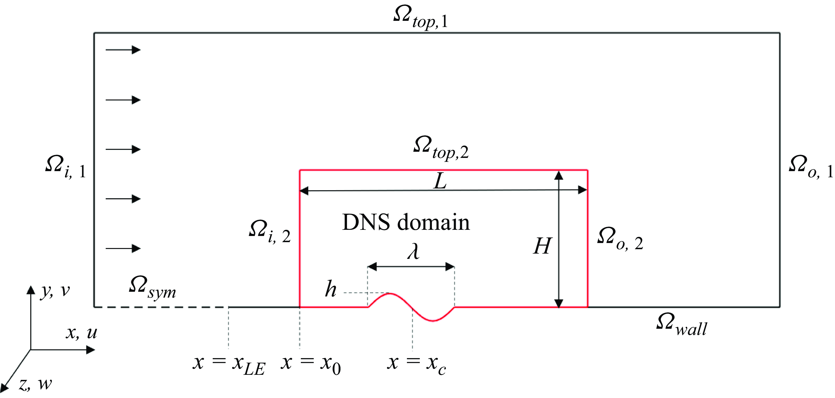
Figure 1. Flow configuration illustrating the two computational domains.
2.1. Governing equations
The non-dimensional Navier–Stokes and continuity equations for an incompressible, constant viscosity flow are
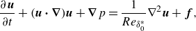 \begin{align}& \frac {\partial \boldsymbol{u}}{\partial t} + (\boldsymbol{u} \boldsymbol{\cdot }\boldsymbol{\nabla }) \boldsymbol{u} + \boldsymbol{\nabla } p = \frac {1}{Re _{\delta _0^*}} \nabla ^2 \boldsymbol{u} + \boldsymbol{f}, \end{align}
 \begin{align}&\qquad\qquad\qquad \boldsymbol{\nabla } \boldsymbol{\cdot }\boldsymbol{u} = 0, \end{align}
where $\boldsymbol{u}=[u,v,w]^T$
are velocity components in Cartesian
$\boldsymbol{u}=[u,v,w]^T$
are velocity components in Cartesian $x$
,
$x$
, $y$
and
$y$
and $z$
directions, respectively,
$z$
directions, respectively, $p$
is the pressure,
$p$
is the pressure, $\boldsymbol{f}$
is the forcing term and
$\boldsymbol{f}$
is the forcing term and $Re _{\delta _0^*}=(U_\infty \delta _0^*)/\nu$
is the Reynolds number based on the reference length,
$Re _{\delta _0^*}=(U_\infty \delta _0^*)/\nu$
is the Reynolds number based on the reference length, $\delta _0^*$
, which is taken as the displacement thickness at
$\delta _0^*$
, which is taken as the displacement thickness at $x=x_0$
;
$x=x_0$
; $U_\infty$
is the free-stream velocity and
$U_\infty$
is the free-stream velocity and $\nu$
is the kinematic viscosity.
$\nu$
is the kinematic viscosity.
For each definition of the wall waviness, two different sets of simulations are performed using the two computational domains shown in figure 1. A preliminary simulation considers the larger domain (denoted by subscript 1) and solves the two-dimensional steady-state form of the Navier–Stokes equations. Uniform velocity ( $u=1$
) at inlet
$u=1$
) at inlet $\Omega _{i,1}$
, free-stream conditions (
$\Omega _{i,1}$
, free-stream conditions ( $u=1, \partial v / \partial y = 0)$
on the top boundary
$u=1, \partial v / \partial y = 0)$
on the top boundary $\Omega _{top,1}$
, no-slip conditions on the wall
$\Omega _{top,1}$
, no-slip conditions on the wall $\Omega _{wall}$
, symmetry boundary condition upstream of the flat plate
$\Omega _{wall}$
, symmetry boundary condition upstream of the flat plate $\Omega _{sym}$
and a standard outflow condition (
$\Omega _{sym}$
and a standard outflow condition ( $p = 0, \partial \boldsymbol{u} / \partial x = 0$
) at the outlet
$p = 0, \partial \boldsymbol{u} / \partial x = 0$
) at the outlet $(\Omega _{o,1})$
are used as boundary conditions for these simulations. The height and downstream extent of the larger domain are checked to be enough to ensure that the pressure on the top and outlet boundaries of the inner domain, i.e.
$(\Omega _{o,1})$
are used as boundary conditions for these simulations. The height and downstream extent of the larger domain are checked to be enough to ensure that the pressure on the top and outlet boundaries of the inner domain, i.e. $p_{top}$
and
$p_{top}$
and $p_{outlet}$
, do not change by further increasing the size of the larger domain. The solutions on the larger domain are computed using the commercial software COMSOL using a
$p_{outlet}$
, do not change by further increasing the size of the larger domain. The solutions on the larger domain are computed using the commercial software COMSOL using a $P_3 - P_2$
finite-element formulation, i.e. third-order elements for the velocity field and second-order elements for the pressure.
$P_3 - P_2$
finite-element formulation, i.e. third-order elements for the velocity field and second-order elements for the pressure.
The rest of the simulations are performed in a reduced computational domain (enclosed by red lines in figure 1), hereafter referred to as the DNS domain, using the spectral element method solver Nek5000 (Deville et al. Reference Deville, Fischer and Mund2002; Fischer et al. Reference Fischer, Lottes and Kerkemeier2008). The $P_N - P_{N-2}$
formulation in Nek5000 with seventh-order elements for velocity and fifth-order elements for pressure is used. In figure 1 the height and length of the DNS domain are denoted by
$P_N - P_{N-2}$
formulation in Nek5000 with seventh-order elements for velocity and fifth-order elements for pressure is used. In figure 1 the height and length of the DNS domain are denoted by $H$
and
$H$
and $L$
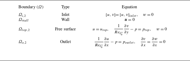
, respectively. The boundary conditions for the DNS domain are summarised in table 1. For three-dimensional simulations, periodic boundary conditions are imposed on the (spanwise) lateral boundaries. For each DNS case (both two- and three-dimensional simulations), the prescribed profiles for
$L$
, respectively. The boundary conditions for the DNS domain are summarised in table 1. For three-dimensional simulations, periodic boundary conditions are imposed on the (spanwise) lateral boundaries. For each DNS case (both two- and three-dimensional simulations), the prescribed profiles for $[u,v]_{inlet}$
,
$[u,v]_{inlet}$
, $[u,p]_{top}$
and
$[u,p]_{top}$
and $p_{outlet}$
(table 1) are obtained from the simulation on the larger domain. Note that, the solutions obtained with COMSOL on the larger domain are only used to provide boundary conditions for DNS simulations. This choice of boundary conditions is based on two reasons: (i) due to the presence of the waviness, the velocity at the inlet might differ from the Blasius solution; and (ii) by setting
$p_{outlet}$
(table 1) are obtained from the simulation on the larger domain. Note that, the solutions obtained with COMSOL on the larger domain are only used to provide boundary conditions for DNS simulations. This choice of boundary conditions is based on two reasons: (i) due to the presence of the waviness, the velocity at the inlet might differ from the Blasius solution; and (ii) by setting $p_{top}$
and
$p_{top}$
and $p_{outlet}$
, the two-dimensional base flows become independent of the height and downstream extent of the DNS domain (Shahriari & Hanifi Reference Shahriari and Hanifi2016). The effect of the waviness on the inlet profiles (for case E – see § 3.2 for the definition of different cases) is shown in figure 2. Finally, a fringe region is added at the outlet of the DNS domain to avoid reflections from the outlet into the domain.
$p_{outlet}$
, the two-dimensional base flows become independent of the height and downstream extent of the DNS domain (Shahriari & Hanifi Reference Shahriari and Hanifi2016). The effect of the waviness on the inlet profiles (for case E – see § 3.2 for the definition of different cases) is shown in figure 2. Finally, a fringe region is added at the outlet of the DNS domain to avoid reflections from the outlet into the domain.
Table 1. Boundary conditions imposed on the DNS domain.
Direct numerical simulations using the smaller domain are performed in this work with different objectives. One is the computation of steady-state solutions of the Navier–Stokes equations to be subsequently subject to linear stability analyses. If the nonlinear system of equations is globally unstable, no steady-state solution can be found using time-marching techniques. Instead, the steady-state solution of the unstable system can be found using techniques such as selective frequency damping (SFD) (Åkervik et al. Reference Åkervik, Brandt, Henningson, Hœpffner, Marxen and Schlatter2006) or Boostconv (Citro et al. Reference Citro, Luchini, Giannetti and Auteri2017). The Boostconv method aims to enhance the convergence of iterative solvers by modifying the part of the eigenspectrum dictated by the unstable or slowly decaying modes. This is achieved by adjusting the residual at each step to ensure faster reduction of the residual in the subsequent iteration. This method is used in this work to find the spanwise-homogeneous two-dimensional base flows, denoted by $\boldsymbol{u}$ $_0=[u_0,v_0,0]^T$
. SFD is used in § 4.2.1 to find the spanwise-modulated fully three-dimensional base flows, denoted by
$_0=[u_0,v_0,0]^T$
. SFD is used in § 4.2.1 to find the spanwise-modulated fully three-dimensional base flows, denoted by $\boldsymbol {u}_{3D}=[u_{3D},v_{3D},w_{3D}]^T$
. SFD adds a forcing term to the momentum equations (using term
$\boldsymbol {u}_{3D}=[u_{3D},v_{3D},w_{3D}]^T$
. SFD adds a forcing term to the momentum equations (using term $f$
in (2.1)) that, in practice, acts as a low-pass filter efficiently damping the unsteadiness present in the flow.
$f$
in (2.1)) that, in practice, acts as a low-pass filter efficiently damping the unsteadiness present in the flow.

2.2. Linearised equations
Considering a steady solution of the governing equations $\bar {\boldsymbol{q}} = [\bar {\boldsymbol{u}},\bar {p}]^T$
as base flow, the linearised Navier–Stokes and continuity equations around
$\bar {\boldsymbol{q}} = [\bar {\boldsymbol{u}},\bar {p}]^T$
as base flow, the linearised Navier–Stokes and continuity equations around $\bar {\boldsymbol{q}}$
can be written as
$\bar {\boldsymbol{q}}$
can be written as
 \begin{align}& \frac {\partial \boldsymbol{u}'}{\partial t} + (\boldsymbol{u}' \boldsymbol{\cdot }\boldsymbol{\nabla })\bar {\boldsymbol{u}} + ( \bar {\boldsymbol{u}} \boldsymbol{\cdot } \boldsymbol{\nabla })\boldsymbol{u}' +\boldsymbol{\nabla } p' = \frac {1}{Re _{\delta _0^*}} \nabla ^2 \boldsymbol{u}', \end{align}
 \begin{align}&\qquad\qquad\qquad\qquad \boldsymbol{\nabla } \boldsymbol{\cdot }\boldsymbol{u}' = 0, \end{align}
where $(')$
denotes perturbation quantities. When the linear solver in Nek5000 is used, to ensure consistency with the boundary conditions satisfied by
$(')$
denotes perturbation quantities. When the linear solver in Nek5000 is used, to ensure consistency with the boundary conditions satisfied by $\bar {\boldsymbol{q}}$
, homogeneous Dirichlet boundary conditions are applied for
$\bar {\boldsymbol{q}}$
, homogeneous Dirichlet boundary conditions are applied for $\boldsymbol{u}$ $'$
on
$'$
on $\Omega _{i,2}$
and
$\Omega _{i,2}$
and $\Omega _{wall}$
, while on
$\Omega _{wall}$
, while on $\Omega _{top,2}$
and
$\Omega _{top,2}$
and $\Omega _{o,2}$
, the respective boundary conditions are
$\Omega _{o,2}$
, the respective boundary conditions are
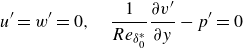 \begin{equation} u'=w'=0, \quad \frac {1}{Re _{\delta _0^*}}\frac {\partial v'}{\partial y} - p' = 0 \end{equation}
and
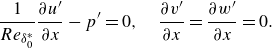 \begin{equation} \frac {1}{Re _{\delta _0^*}}\frac {\partial u'}{\partial x} - p' = 0, \quad \frac {\partial v'}{\partial x} = \frac {\partial w'}{\partial x} = 0. \end{equation}
2.3. Modal stability analysis
Considering modal analysis, the perturbations are written in the form of
 \begin{equation} \boldsymbol{q}'(x,y,z,t) = \hat {\boldsymbol{q}}(x,y,z)e^{-i{\Lambda t}} + c.c., \end{equation}
where $\Lambda =\omega + i\sigma$
and
$\Lambda =\omega + i\sigma$
and $c.c.$
denotes the complex conjugate. By substituting (2.7) into (2.3) and (2.4), a generalized eigenvalue problem of the form
$c.c.$
denotes the complex conjugate. By substituting (2.7) into (2.3) and (2.4), a generalized eigenvalue problem of the form
 \begin{equation} \unicode{x1D647} \hat {\boldsymbol{q}}=\Lambda \unicode{x1D64D} \hat {\boldsymbol{q}} \end{equation}
is found, where
 \begin{equation} \unicode{x1D64D} = \begin{pmatrix} \unicode{x1D644} & 0\\ 0 & 0 \\ \end{pmatrix}, \quad \unicode{x1D647} = \begin{pmatrix} -\boldsymbol{\nabla }\bar {\boldsymbol{u}} - \bar {\boldsymbol{u}} \boldsymbol{\cdot }\boldsymbol{\nabla } + \frac {1}{Re _{\delta _0^*}} \nabla ^2 & -\boldsymbol{\nabla } \\ \boldsymbol{\nabla }\boldsymbol{\cdot }& 0 \\ \end{pmatrix}. \end{equation}
The eigenvalues $\Lambda = \omega + i\sigma$
determine the asymptotic behaviour of the system to small amplitude disturbances, where
$\Lambda = \omega + i\sigma$
determine the asymptotic behaviour of the system to small amplitude disturbances, where $\sigma$
and
$\sigma$
and $\omega$
are the exponential growth rate and frequency of perturbations, respectively. If
$\omega$
are the exponential growth rate and frequency of perturbations, respectively. If $\sigma \gt 0$
, the system is globally unstable and any small amplitude perturbation will grow exponentially over time.
$\sigma \gt 0$
, the system is globally unstable and any small amplitude perturbation will grow exponentially over time.
To obtain the two-dimensional global modes of the two-dimensional base flows $\bar {\boldsymbol{q}}$
, a matrix-free approach (Bagheri et al. Reference Bagheri, Åkervik, Brandt and Henningson2009) is employed that uses the implicitly restarted Arnoldi method (Lehoucq et al. Reference Lehoucq, Sorensen and Yang1998) implemented in Nek5000. In this case, the two-dimensional base flows (
$\bar {\boldsymbol{q}}$
, a matrix-free approach (Bagheri et al. Reference Bagheri, Åkervik, Brandt and Henningson2009) is employed that uses the implicitly restarted Arnoldi method (Lehoucq et al. Reference Lehoucq, Sorensen and Yang1998) implemented in Nek5000. In this case, the two-dimensional base flows ( $\boldsymbol{u_0}$
) are obtained with Nek5000 (on the DNS domain) using Boostconv. The base flows will be introduced in § 3.2, while the stability analysis results corresponding to this part are presented in § 4.1.
$\boldsymbol{u_0}$
) are obtained with Nek5000 (on the DNS domain) using Boostconv. The base flows will be introduced in § 3.2, while the stability analysis results corresponding to this part are presented in § 4.1.

Figure 3. Mapping of the physical domain to the computational domain used in the matrix-forming eigenvalue analysis. The computational domain corresponds to the shaded area of the physical domain.
To obtain the three-dimensional global modes of two-dimensional base flows, a matrix-forming approach is used. The base flows here are obtained by interpolating the base flows calculated using Nek5000 on a smaller subdomain (shaded area in figure 3). In this case, instead of solving the three-dimensional eigenvalue problem, perturbations can be assumed to be periodic in the spanwise direction, with spanwise wavenumber $\beta$
. In this case, the ansatz (2.7) is rewritten as
$\beta$
. In this case, the ansatz (2.7) is rewritten as
 \begin{equation} \boldsymbol{q}'(x,y,z,t) = \hat {\boldsymbol{q}}(x,y)e^{i(\beta z - {\Lambda t})} + c.c. \end{equation}
By substituting the ansatz (2.10) into (2.3) and (2.4), a generalized eigenvalue problem similar to (2.8) is obtained. The corresponding terms for linear operators $\unicode{x1D647}$
and
$\unicode{x1D647}$
and $\unicode{x1D64D}$
of the resulting eigenvalue problem can be found in Rodríguez & Theofilis (Reference Rodríguez and Theofilis2009). Fourth-order central finite differences are used to discretise the derivatives of the operators. Moreover, in order to account for the curvature of the geometry as well as non-orthogonal grids, the analytical mapping
$\unicode{x1D64D}$
of the resulting eigenvalue problem can be found in Rodríguez & Theofilis (Reference Rodríguez and Theofilis2009). Fourth-order central finite differences are used to discretise the derivatives of the operators. Moreover, in order to account for the curvature of the geometry as well as non-orthogonal grids, the analytical mapping
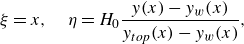 \begin{equation} \xi = x, \quad \eta = {H_0}\dfrac {y(x)-y_w(x)}{y_{top}(x) - y_w(x)}, \end{equation}
is used to map the physical domain $(x,y)$
into the computational one
$(x,y)$
into the computational one ${(\xi, \eta })$
as shown in figure 3. Homogeneous Dirichlet boundary conditions are imposed for perturbations at the inlet, top boundary of the computation domain and at the wall, while homogeneous Neumann boundary conditions are imposed at the outlet of the domain. In (2.11),
${(\xi, \eta })$
as shown in figure 3. Homogeneous Dirichlet boundary conditions are imposed for perturbations at the inlet, top boundary of the computation domain and at the wall, while homogeneous Neumann boundary conditions are imposed at the outlet of the domain. In (2.11), $H_0$
is the height of the subdomain, while
$H_0$
is the height of the subdomain, while $y_w(x)$
and
$y_w(x)$
and $y_{top}(x)$
are the coordinates of the wall and top boundary in the physical domain, respectively. Note that the top boundary of the physical subdomain chosen for the eigenvalue problem (grey area in figure 3) is formed by simply moving the shape of the wall
$y_{top}(x)$
are the coordinates of the wall and top boundary in the physical domain, respectively. Note that the top boundary of the physical subdomain chosen for the eigenvalue problem (grey area in figure 3) is formed by simply moving the shape of the wall $H_0$
units in the
$H_0$
units in the $y$
direction. This particular choice of the top boundary of subdomain for eigenvalue analysis guarantees an orthogonal grid in the computational domain, and both the physical and computational domains will have the same grid clustering near the wall without any further transformations.
$y$
direction. This particular choice of the top boundary of subdomain for eigenvalue analysis guarantees an orthogonal grid in the computational domain, and both the physical and computational domains will have the same grid clustering near the wall without any further transformations.
Finally, the resulting two-dimensional eigenvalue problem is solved in parallel with sparse linear-algebra techniques using the shift-and-invert Krylov–Schur algorithm implemented in SLEPc (Hernandez et al. Reference Hernandez, Roman and Vidal2005). Also, the MUMPS package (Amestoy et al. Reference Amestoy, Duff, L’Excellent and Koster2000) is used for performing the lower–upper decomposition of the sparse matrices. The results corresponding to this section are presented in § 4.2. This approach is validated with Nek5000 as shown in Appendix A.2.
3. Two-dimensional base flows
This section first presents a scaling to predict the onset of flow separation for the sinusoidal waviness considered in this work (§ 3.1). Based on that, several flow cases are considered for further analysis, which are introduced in § 3.2.
3.1. Onset of flow separation
The wall waviness presents two consecutive changes in curvature that introduce favourable pressure gradient and APG regions, and cause flow separation if the intensity of the APG is large enough. Different works proposed boundary layer separation criteria based on dimensionless parameters that consider the thickness of the boundary layer, the kinematic viscosity and a measure of the streamwise velocity gradient at the boundary layer edge (Thwaites Reference Thwaites1949; Gaster Reference Gaster1966); thus, a priori knowledge of velocity profiles is required. Ultimately, these quantities are a consequence of the geometrical parameters of the waviness ( $h,\lambda$
) and the Reynolds number based on the boundary layer thickness. This suggests an alternative criterion for the prediction of the boundary layer separation for the present configuration, based on the dimensionless numbers
$h,\lambda$
) and the Reynolds number based on the boundary layer thickness. This suggests an alternative criterion for the prediction of the boundary layer separation for the present configuration, based on the dimensionless numbers $h/\delta$
and
$h/\delta$
and $Re _{\delta _{x_c}^*}={(U_\infty {\delta _{x_c}^*})}/{\nu }$
. Here
$Re _{\delta _{x_c}^*}={(U_\infty {\delta _{x_c}^*})}/{\nu }$
. Here $\delta$
and
$\delta$
and $\delta ^*$
are the boundary layer and displacement thickness of the corresponding Blasius solution at
$\delta ^*$
are the boundary layer and displacement thickness of the corresponding Blasius solution at $x = x_c$
, respectively. To find such a dependence, the wavelength
$x = x_c$
, respectively. To find such a dependence, the wavelength $\lambda$
for which the wall shear stress vanishes has been determined for simulations with different Reynolds numbers and waviness heights. These are shown in the left panel of figure 4. Next, all the curves are scaled with
$\lambda$
for which the wall shear stress vanishes has been determined for simulations with different Reynolds numbers and waviness heights. These are shown in the left panel of figure 4. Next, all the curves are scaled with $(Re _{\delta _{x_c}^*})^{0.5}$
, obtaining an excellent collapse as shown in the right panel of figure 4. Then, a power-law curve is fitted to the data to obtain an equation to predict the waviness parameters that causes flow separation:
$(Re _{\delta _{x_c}^*})^{0.5}$
, obtaining an excellent collapse as shown in the right panel of figure 4. Then, a power-law curve is fitted to the data to obtain an equation to predict the waviness parameters that causes flow separation:
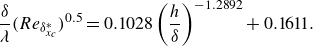 \begin{equation} \frac {\delta }{\lambda }(Re _{\delta _{x_c}^*})^{0.5}=0.1028\left (\frac {h}{\delta }\right )^{-1.2892}+0.1611. \end{equation}
For any combination of parameters that lies above this curve, flow separation is expected to happen.
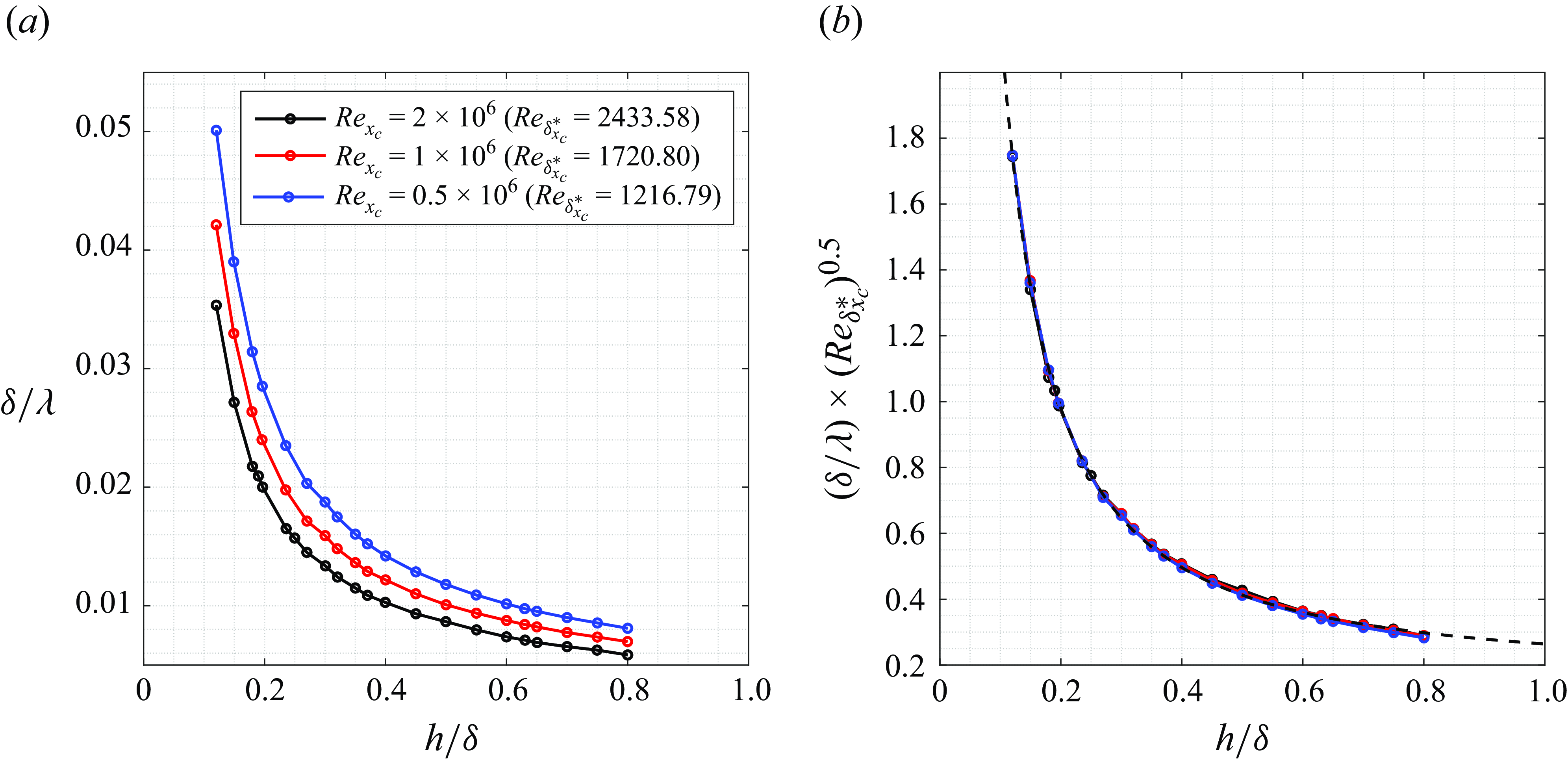
Figure 4. Scaling of waviness parameters for incipient separation.
Table 2. Geometrical parameters defining the cases considered in this work.
3.2. Base flow cases
Equation (3.1) allows constructing different geometries resulting in LSBs with different (not known a priori) length, thickness and reverse flow intensity. For all the geometries considered in the rest of this work, the Reynolds number based on local Blasius displacement thickness at the centre of the waviness is $Re _{\delta _{x_c}^*}=1720.8$
, which corresponds to
$Re _{\delta _{x_c}^*}=1720.8$
, which corresponds to $Re _{{x_c}}={(U_\infty x_c)}/{\nu }=1 \times 10^6$
. For all cases, the location of the inlet
$Re _{{x_c}}={(U_\infty x_c)}/{\nu }=1 \times 10^6$
. For all cases, the location of the inlet $(x=x_0)$
is chosen such that the Reynolds number based on the local Blasius displacement thickness is
$(x=x_0)$
is chosen such that the Reynolds number based on the local Blasius displacement thickness is $Re _{\delta _{x_0}^*}=1332.925$
. The value of
$Re _{\delta _{x_0}^*}=1332.925$
. The value of $\delta _{x_0}^*$
is taken as the reference length to make all coordinates non-dimensional. Finally, the origin of the dimensionless streamwise coordinate is displaced to the inlet of the DNS computational domain, so that
$\delta _{x_0}^*$
is taken as the reference length to make all coordinates non-dimensional. Finally, the origin of the dimensionless streamwise coordinate is displaced to the inlet of the DNS computational domain, so that $x=0$
is the inlet coordinate and
$x=0$
is the inlet coordinate and $x_c \approx 300$
. For reference, the dimensionless Blasius boundary layer thickness at
$x_c \approx 300$
. For reference, the dimensionless Blasius boundary layer thickness at $x_c$
is
$x_c$
is $\delta _{x_c}=3.7512$
. Table 2 summarises the geometrical parameters for different geometries considered; these cases are also shown on the separation diagram in figure 5. Separated flow is present for all cases except case B, which is at the edge of separation. Note that, all two-dimensional base flows are obtained with a DNS domain size of
$\delta _{x_c}=3.7512$
. Table 2 summarises the geometrical parameters for different geometries considered; these cases are also shown on the separation diagram in figure 5. Separated flow is present for all cases except case B, which is at the edge of separation. Note that, all two-dimensional base flows are obtained with a DNS domain size of $H=700$
and
$H=700$
and $L=1400$
.
$L=1400$
.
Figure 5. Geometrical parameters defining the cases considered in this work. The dashed line shows the separation curve for $Re _{\delta _{x_c}^*}=1720.8$
.
$Re _{\delta _{x_c}^*}=1720.8$
.
Figure 6. Base flows for cases A, C and E. The colour map corresponds to streamwise velocity $u$
. Here
$u$
. Here ${\rm d}C_p/{\rm d}s$
is shown by a dashed black line and the values are indicated by the right vertical axis. White and red dashed lines show reverse flow
${\rm d}C_p/{\rm d}s$
is shown by a dashed black line and the values are indicated by the right vertical axis. White and red dashed lines show reverse flow $y_r$
and dividing streamlines
$y_r$
and dividing streamlines $y_d$
, respectively. The figure is not drawn to scale.
$y_d$
, respectively. The figure is not drawn to scale.
Figure 6 shows the streamwise velocity $u$
for cases A, C and E. The figure is not drawn to scale in order to enhance the visibility of the recirculation bubble. The derivative of the pressure coefficient
$u$
for cases A, C and E. The figure is not drawn to scale in order to enhance the visibility of the recirculation bubble. The derivative of the pressure coefficient $C_p$
with respect to the wall arc length
$C_p$
with respect to the wall arc length $s$
,
$s$
, $dC_p/ds$
, is shown by the dashed black line. The red dashed line shows the dividing streamline
$dC_p/ds$
, is shown by the dashed black line. The red dashed line shows the dividing streamline $y_d$
, defined as the
$y_d$
, defined as the $y$
coordinate below which the streamwise mass flux is zero, i.e.
$y$
coordinate below which the streamwise mass flux is zero, i.e. $\int _{y_{wall}}^{y_d}u(x,y){\rm d}y=0$
. The white dashed line corresponds to the coordinate
$\int _{y_{wall}}^{y_d}u(x,y){\rm d}y=0$
. The white dashed line corresponds to the coordinate $y_r$
that delimits the reverse flow region (
$y_r$
that delimits the reverse flow region ( $u\lt 0$
). Table 3 summarises different characteristics of the separation bubble for all cases.
$u\lt 0$
). Table 3 summarises different characteristics of the separation bubble for all cases.
Table 3. Maximum reverse flow $(u_{rev})$
,
$(u_{rev})$
, $x$
coordinate of separation
$x$
coordinate of separation $(x_s)$
and reattachment
$(x_s)$
and reattachment $(x_r)$
points, length of separation bubble
$(x_r)$
points, length of separation bubble $(L_s = x_r - x_s)$
, momentum thickness at separation point
$(L_s = x_r - x_s)$
, momentum thickness at separation point $(\theta _s)$
, maximum vertical distance between the wall and dividing streamline
$(\theta _s)$
, maximum vertical distance between the wall and dividing streamline $(h_1)$
, maximum vertical distance between the wall and separation point
$(h_1)$
, maximum vertical distance between the wall and separation point $(h_2)$
, Reynolds number based on momentum thickness at the separation point (
$(h_2)$
, Reynolds number based on momentum thickness at the separation point ( $Re _{\theta, s}$
) and Reynolds number based on the length of the separation bubble
$Re _{\theta, s}$
) and Reynolds number based on the length of the separation bubble $(Re _{L})$
. For all cases,
$(Re _{L})$
. For all cases, $Re _{\delta _{x_c}^*}=1720.8$
.
$Re _{\delta _{x_c}^*}=1720.8$
.
Figure 6, illustrates how the change of wall curvature, especially near the reattachment, plays a significant role in the shape and length of the separation bubble. The flow experiences an acceleration in the first part of the waviness, followed by an APG region that results in flow separation. A pressure plateau is evident within the recirculating region, except for the proximity of the reattachment region. For cases A and E, near the rear end of the bubble the flow experiences a sudden deceleration and the dividing streamline bends towards the wall. The reattachment occurs either at the end point of the wall waviness or downstream, in the flat plate. After reattachment, the flow accelerates until a zero pressure gradient region is recovered over the flat plate. Conversely, in case C where the reattachment is upstream of the end of the waviness, the flow experiences an acceleration after the reattachment.
Regarding the maximum value of reverse flow, both $h$
and
$h$
and $\lambda$
play a role. This can be seen by comparing maximum reverse flow magnitude for cases G, E and H, where
$\lambda$
play a role. This can be seen by comparing maximum reverse flow magnitude for cases G, E and H, where $h/\lambda$
is the same; however, the reverse flows are different. The reverse flow increases by increasing the height of waviness while keeping constant
$h/\lambda$
is the same; however, the reverse flows are different. The reverse flow increases by increasing the height of waviness while keeping constant $\lambda$
. At a constant height of the waviness, increasing
$\lambda$
. At a constant height of the waviness, increasing $h/\lambda$
(i.e. decreasing
$h/\lambda$
(i.e. decreasing $\lambda$
), increases the reverse flow magnitude. The effect of height of the waviness is found to be more pronounced:
$\lambda$
), increases the reverse flow magnitude. The effect of height of the waviness is found to be more pronounced: $h/\lambda$
for case A is almost
$h/\lambda$
for case A is almost $16\,\%$
higher than that for case H, but case H has a higher maximum reverse flow than case A.
$16\,\%$
higher than that for case H, but case H has a higher maximum reverse flow than case A.
The wall curvature also affects the streamlines of the flow, especially near the rear part of the waviness where the flow undergoes a sudden deceleration. This is shown in figure 7 that depicts the streamlines for cases G, A, E and H. Among the four cases shown in this figure, the curvature of the streamlines in case G does not change sign inside the recirculation bubble. The same happens for cases C, D and F (not shown here). On the other hand, the curvature of streamlines in cases A, E, H and I (not shown here) changes sign in the vicinity of the reattachment point. This change in the sign of streamline curvature is found to directly impact the three-dimensional global centrifugal instabilities, as will be discussed in § 4.2. Note that in the base flow for case H a second recirculation region inside the main one is formed, as shown in figure 7(e). The same streamline topology has been reported for different two-dimensional steady solutions of the Navier–Stokes equations recovering fully laminar recirculation bubbles (e.g. Alizard et al. Reference Alizard, Cherubini and Robinet2009; Balzer & Fasel Reference Balzer and Fasel2016). This seems to be an effect of the rapid increase of pressure gradient near the reattachment point. In what follows, the spanwise-homogeneous (two-dimensional) base flows presented in this section will be referred to by $\boldsymbol{u}_0=[u_0,v_0,0]^T$
.
$\boldsymbol{u}_0=[u_0,v_0,0]^T$
.
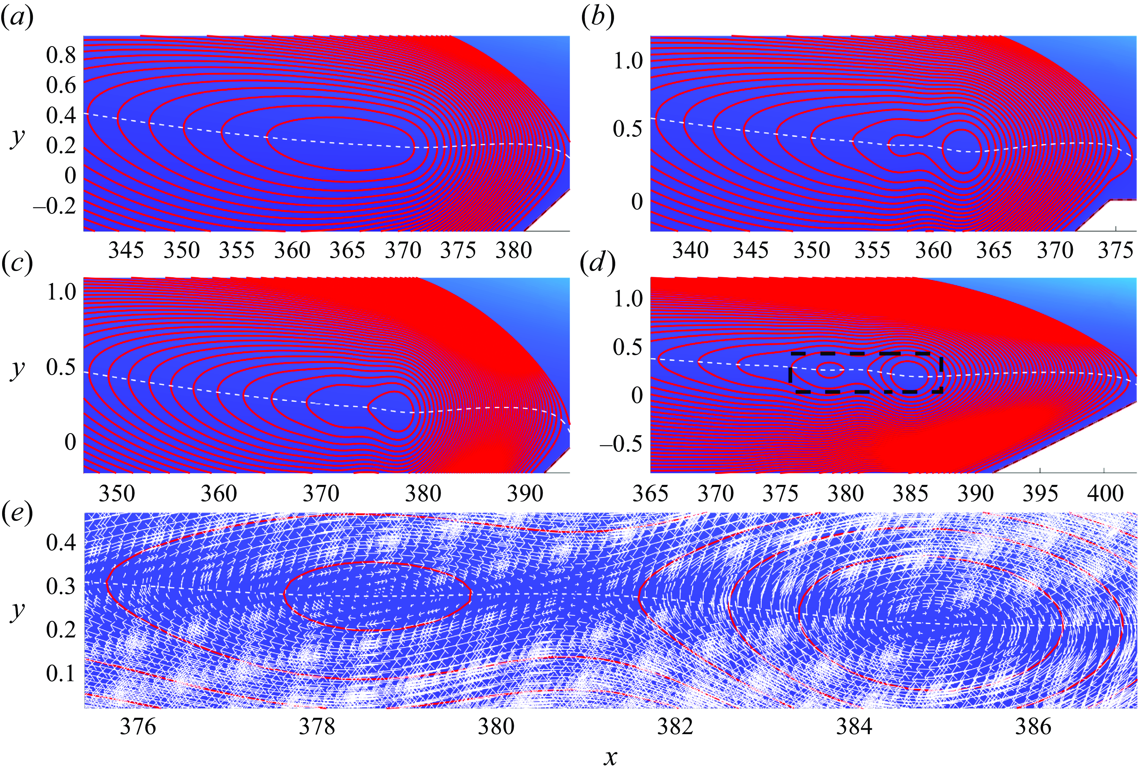
Figure 7. Flow streamlines near reattachment point for cases (a) G, (b) A, (c) E and (d) H. The figure is not drawn to scale. (e) Velocity vectors within the marked dashed rectangular region in case H.
4. Primary instability analysis of the two-dimensional base flows
4.1. Two-dimensional instability: vortex shedding
In this section the results for global stability analysis for two-dimensional perturbations (introduced in § 2.3) are presented. The numerical details and domain sensitivity analysis are given in Appendix A.1. Figure 8 shows the eigenspectra for all the cases. Note that the eigenspectrum being symmetric about $\omega = 0$
, only the side of it with positive frequencies is shown. The eigenspectra show two different families of eigenmodes, characterised as low-frequency (
$\omega = 0$
, only the side of it with positive frequencies is shown. The eigenspectra show two different families of eigenmodes, characterised as low-frequency ( $\omega \lt 0.06$
) and high-frequency (
$\omega \lt 0.06$
) and high-frequency ( $\omega \gt 0.06$
) regions, respectively. For case B, which is the case without flow separation, only the low-frequency part of the eigenspectrum appears. Among all cases studied, only cases E, F and H are globally unstable with respect to two-dimensional instabilities; a self-sustained oscillator-type instability is expected to happen for these cases in nonlinear simulations without external forcing. The peak reverse flow for these unstable cases is
$\omega \gt 0.06$
) regions, respectively. For case B, which is the case without flow separation, only the low-frequency part of the eigenspectrum appears. Among all cases studied, only cases E, F and H are globally unstable with respect to two-dimensional instabilities; a self-sustained oscillator-type instability is expected to happen for these cases in nonlinear simulations without external forcing. The peak reverse flow for these unstable cases is $u_{rev}\approx 10-12\,\%$
, which is lower than the threshold of
$u_{rev}\approx 10-12\,\%$
, which is lower than the threshold of $u_{rev}\approx 16 \,\%$
(Rist & Maucher Reference Rist and Maucher2002; Alam & Sandham Reference Alam and Sandham2000), and the inflection point does not cross the dividing streamlines of these bubbles (as proposed by Avanci et al. Reference Avanci, Rodríguez and Alves2019), suggesting that the global instability does not originate from the local absolute inflectional instability, but by fully non-parallel effects.
$u_{rev}\approx 16 \,\%$
(Rist & Maucher Reference Rist and Maucher2002; Alam & Sandham Reference Alam and Sandham2000), and the inflection point does not cross the dividing streamlines of these bubbles (as proposed by Avanci et al. Reference Avanci, Rodríguez and Alves2019), suggesting that the global instability does not originate from the local absolute inflectional instability, but by fully non-parallel effects.

Figure 8. Eigenspectra of two-dimensional global eigenmodes ( $\beta = 0$
) of the two-dimensional base flows.
$\beta = 0$
) of the two-dimensional base flows.
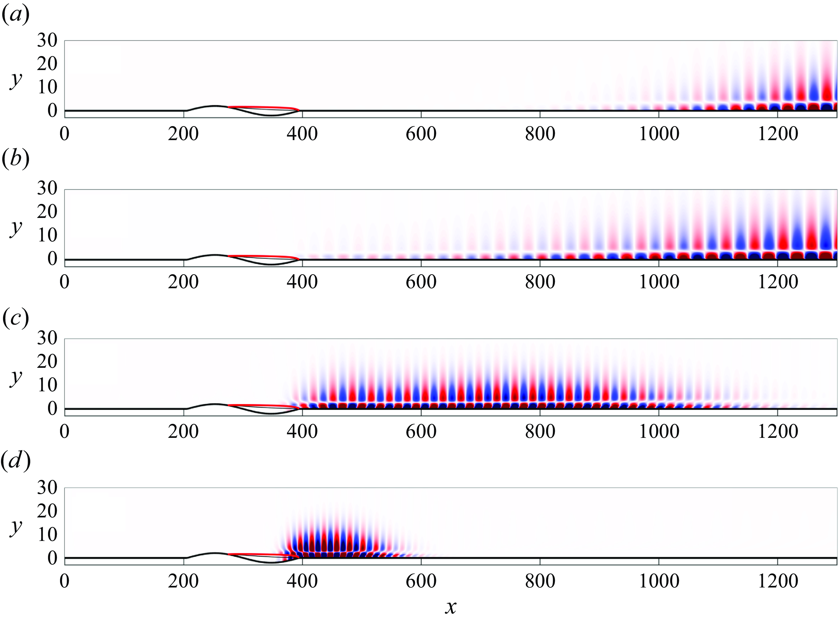
Figure 9. Real part of the streamwise velocity component of global eigenmodes for case E, corresponding to the four eigenvalues marked with the letters $a$
,
$a$
, $b$
,
$b$
, $c$
and
$c$
and $d$
in figure 8.
$d$
in figure 8.
The growth rate and frequency of high-frequency modes show a higher sensitivity to the geometry of the waviness. This is in agreement with the results of Ehrenstein & Gallaire (Reference Ehrenstein and Gallaire2008) for a separated flow over a hump. Figure 9 shows the real part of the streamwise velocity component of global modes for case E, corresponding to the four eigenvalues marked with the letters $a$
,
$a$
, $b$
,
$b$
, $c$
and
$c$
and $d$
in figure 8. Figure 9 confirms that that low-frequency and high-frequency modes belong to different families. Low-frequency modes, corresponding to convectively unstable waves, resemble Tollmien–Schlichting waves downstream of the wall waviness. The corresponding eigenfunctions are also similar to eigenfunctions of a family of low-frequency modes found downstream of the reattachment point of an LSB caused by a smooth hump, as shown by Ehrenstein & Gallaire (Reference Ehrenstein and Gallaire2008). The modes in the high-frequency family exhibit a notable spatial amplification in the separated shear layer and inside the recirculation region, upstream of the reattachment point. The spatial shape of all the high-frequency modes (either stable or unstable) shares the same features; however, their spatial extension downstream of the reattachment point decreases from eigenmode to eigenmode as their frequency increases (modes
$d$
in figure 8. Figure 9 confirms that that low-frequency and high-frequency modes belong to different families. Low-frequency modes, corresponding to convectively unstable waves, resemble Tollmien–Schlichting waves downstream of the wall waviness. The corresponding eigenfunctions are also similar to eigenfunctions of a family of low-frequency modes found downstream of the reattachment point of an LSB caused by a smooth hump, as shown by Ehrenstein & Gallaire (Reference Ehrenstein and Gallaire2008). The modes in the high-frequency family exhibit a notable spatial amplification in the separated shear layer and inside the recirculation region, upstream of the reattachment point. The spatial shape of all the high-frequency modes (either stable or unstable) shares the same features; however, their spatial extension downstream of the reattachment point decreases from eigenmode to eigenmode as their frequency increases (modes $c$
and
$c$
and $d$
). The eigenmodes shown in figure 9 are similar to the two-dimensional eigenmodes found in the LSBs caused by a smooth cavity (Åkervik et al. Reference Åkervik, Hœpffner, Ehrenstein and Henningson2007) and smooth hump (Ehrenstein & Gallaire Reference Ehrenstein and Gallaire2008).
$d$
). The eigenmodes shown in figure 9 are similar to the two-dimensional eigenmodes found in the LSBs caused by a smooth cavity (Åkervik et al. Reference Åkervik, Hœpffner, Ehrenstein and Henningson2007) and smooth hump (Ehrenstein & Gallaire Reference Ehrenstein and Gallaire2008).
4.2. Three-dimensional instability: base flow three-dimensionalisation
Since the base flows $\boldsymbol{u}_0$
are homogeneous in the
$\boldsymbol{u}_0$
are homogeneous in the $z$
direction, their three-dimensional instability is studied using global stability analysis of perturbations of the form (2.10). Details of the numerical set-up and cross-validations using Nek5000 are given in Appendix A.2.
$z$
direction, their three-dimensional instability is studied using global stability analysis of perturbations of the form (2.10). Details of the numerical set-up and cross-validations using Nek5000 are given in Appendix A.2.
For an LSB on a flat plate, Theofilis et al. (Reference Theofilis, Hein and Dallmann2000) reported the existence of a single steady unstable centrifugal three-dimensional eigenmode for a specific spanwise wavenumber. Recently, Rodríguez et al. (Reference Rodríguez, Gennaro and Souza2021a
) showed that this eigenmode is responsible for spanwise modulation of an initially two-dimensional base flow and can potentially lead to transition through a self-excited secondary instability mechanism. Here, on a curved surface, we show that for a specific $\beta$
, more than one zero-frequency unstable centrifugal mode can coexist. The effect of spanwise wavenumber on the growth rate of the leading unstable eigenmode(s) is shown, for all cases, in figure 10. Note that all the eigenmodes shown in this figure have zero frequency. In the case of having two unstable eigenmodes for a specific
$\beta$
, more than one zero-frequency unstable centrifugal mode can coexist. The effect of spanwise wavenumber on the growth rate of the leading unstable eigenmode(s) is shown, for all cases, in figure 10. Note that all the eigenmodes shown in this figure have zero frequency. In the case of having two unstable eigenmodes for a specific $\beta$
, the lower-growth-rate modes are shown by the same symbol as the higher-growth-rate modes, but are connected with a dashed line. No more than two unstable eigenmodes have been found in any of the cases.
$\beta$
, the lower-growth-rate modes are shown by the same symbol as the higher-growth-rate modes, but are connected with a dashed line. No more than two unstable eigenmodes have been found in any of the cases.
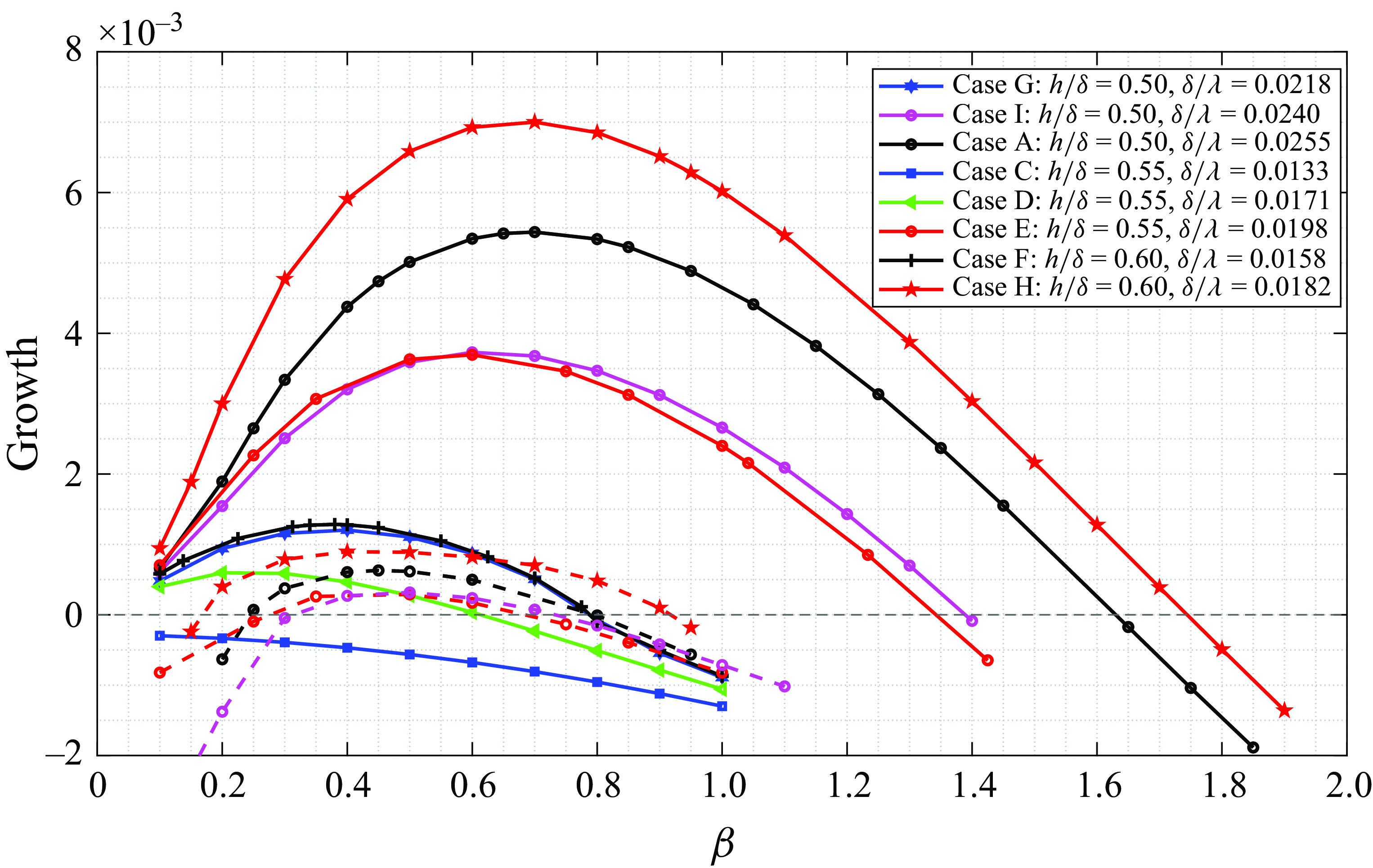
Figure 10. Dependence of the maximum growth rate of steady ( $\omega =0$
) eigenmodes on the spanwise wavenumber for different cases. In the case of coexistence of two eigenmodes at one spanwise wavenumber, the growth rate of the second mode is shown by a dashed line.
$\omega =0$
) eigenmodes on the spanwise wavenumber for different cases. In the case of coexistence of two eigenmodes at one spanwise wavenumber, the growth rate of the second mode is shown by a dashed line.
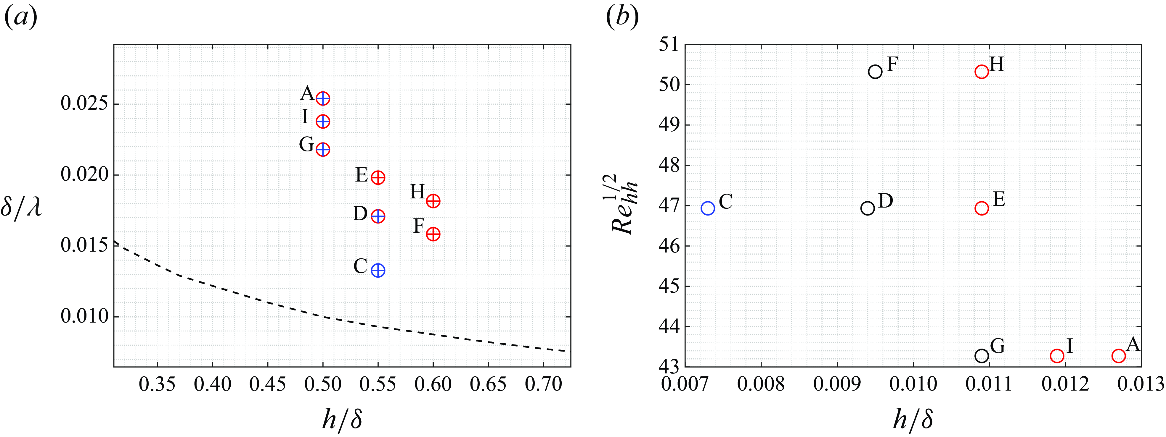
Figure 11. (a) Stability diagram in $h/\delta$
–
$h/\delta$
– $\delta / \lambda$
parameter space. Plus and circles show the stability characteristics of two- and three-dimensional instabilities, respectively (blue: stable, red: unstable). The black dashed line shows the separation curve for
$\delta / \lambda$
parameter space. Plus and circles show the stability characteristics of two- and three-dimensional instabilities, respectively (blue: stable, red: unstable). The black dashed line shows the separation curve for $Re _{\delta _{x_c}^*}=1720.8$
(see figure 5). (b) Stability diagram of three-dimensional instabilities in the
$Re _{\delta _{x_c}^*}=1720.8$
(see figure 5). (b) Stability diagram of three-dimensional instabilities in the $Re ^{1/2}_{hh}$
–
$Re ^{1/2}_{hh}$
– $h / \lambda$
parameter space. The blue circle shows the stable case, black circles show the cases with one unstable eigenvalue and red circles show the cases where two unstable eigenvalues are present for a particular value of
$h / \lambda$
parameter space. The blue circle shows the stable case, black circles show the cases with one unstable eigenvalue and red circles show the cases where two unstable eigenvalues are present for a particular value of $\beta$
.
$\beta$
.
Figure 11 summarises the stable and unstable cases in two different parameter spaces. Figure 11(a) shows the stability characteristics of cases in $h/\delta$
–
$h/\delta$
– $\delta / \lambda$
parameter space, where the plus and circle symbols are for two- and three-dimensional instabilities, respectively. Blue and red colours also show stable and unstable cases, respectively. From the figure it is clear that, at a fixed height of the waviness, by decreasing the wavelength of the waviness, i.e. increasing
$\delta / \lambda$
parameter space, where the plus and circle symbols are for two- and three-dimensional instabilities, respectively. Blue and red colours also show stable and unstable cases, respectively. From the figure it is clear that, at a fixed height of the waviness, by decreasing the wavelength of the waviness, i.e. increasing $\delta / \lambda$
, three-dimensional instabilities become unstable prior to two-dimensional instabilities. Figure 11 (b) shows the stability characteristics of three-dimensional instabilities in the
$\delta / \lambda$
, three-dimensional instabilities become unstable prior to two-dimensional instabilities. Figure 11 (b) shows the stability characteristics of three-dimensional instabilities in the $Re ^{1/2}_{hh}$
–
$Re ^{1/2}_{hh}$
– $h / \lambda$
parameter space, where
$h / \lambda$
parameter space, where $Re _{hh}=u(h)h/\nu$
is the local Reynolds number at the
$Re _{hh}=u(h)h/\nu$
is the local Reynolds number at the $x$
location of the maximum height of the waviness
$x$
location of the maximum height of the waviness $h$
and
$h$
and $u(h)$
is the value of the Blasius velocity profile at height
$u(h)$
is the value of the Blasius velocity profile at height $h$
(Von Doenhoff & Braslow Reference Von, Albert and Braslow1961; Bucci et al. Reference Bucci, Cherubini, Loiseau and Robinet2021). Although analysing more cases is required to properly identify the neutral curves at this parameter space, from the figure it is clear that at a fixed
$h$
(Von Doenhoff & Braslow Reference Von, Albert and Braslow1961; Bucci et al. Reference Bucci, Cherubini, Loiseau and Robinet2021). Although analysing more cases is required to properly identify the neutral curves at this parameter space, from the figure it is clear that at a fixed $Re _{hh}$
, by increasing the aspect ratio
$Re _{hh}$
, by increasing the aspect ratio $h / \lambda$
of the waviness, first the flows become unstable with respect to one unstable global mode (black circles) and then with respect to two global eigenmdoes (red circles) for a fixed value of spanwise wavenumber.
$h / \lambda$
of the waviness, first the flows become unstable with respect to one unstable global mode (black circles) and then with respect to two global eigenmdoes (red circles) for a fixed value of spanwise wavenumber.
The existence of multiple steady centrifugal eigenmodes is found to be directly related to the number of sign changes in the curvature of the recirculating streamlines of the base flow. As explained in § 3.2 and shown in figure 7, cases A, E, H and I present more than one change of curvature sign due to the presence of the curved wall. For these four cases, as figure 10 shows, the coexistence of two unstable centrifugal modes is possible in a finite range of $\beta$
. Note that the unstable range of
$\beta$
. Note that the unstable range of $\beta$
for the higher-growth-rate eigenmode is almost twice that for the lower-growth-rate mode.
$\beta$
for the higher-growth-rate eigenmode is almost twice that for the lower-growth-rate mode.
Figure 12 shows the real part of the streamwise $u$
(left panels) and
$u$
(left panels) and $v$
(right panels) velocity components for the two unstable eigenmodes of case A with
$v$
(right panels) velocity components for the two unstable eigenmodes of case A with $\beta =0.7$
, and the single unstable eigenmode for case G with
$\beta =0.7$
, and the single unstable eigenmode for case G with $\beta =0.4$
; the top and middle panels show the eigenfunctions for the higher-growth-rate (M1) and lower-growth-rate mode (M2) for case A, and the bottom panels show the same eigenfunctions for the unstable mode (M1) in case G. Flow streamlines in the vicinity of the change of streamline curvature are also plotted as thin grey lines in the figure. The higher-growth-rate mode is very localised in the region where the curvature of streamlines changes. For a given
$\beta =0.4$
; the top and middle panels show the eigenfunctions for the higher-growth-rate (M1) and lower-growth-rate mode (M2) for case A, and the bottom panels show the same eigenfunctions for the unstable mode (M1) in case G. Flow streamlines in the vicinity of the change of streamline curvature are also plotted as thin grey lines in the figure. The higher-growth-rate mode is very localised in the region where the curvature of streamlines changes. For a given $\beta$
, the growth rate of this mode, which will be referred to as the localised mode, is one order of magnitude higher than that of the other mode, which will be referred to as the spread mode. It should be noted that, at a fixed
$\beta$
, the growth rate of this mode, which will be referred to as the localised mode, is one order of magnitude higher than that of the other mode, which will be referred to as the spread mode. It should be noted that, at a fixed $h/\delta$
when both the localised and spread modes coexist, the growth rate of both modes increases with decreasing wavelength of the waviness, i.e. increasing
$h/\delta$
when both the localised and spread modes coexist, the growth rate of both modes increases with decreasing wavelength of the waviness, i.e. increasing $\delta / \lambda$
, as can be seen from figure 10 (cases A and I). The spatial structure of the spread mode extends over the whole recirculation bubble and shares the same features as the three-dimensional global mode found in LSBs formed on a flat plate (Theofilis et al. Reference Theofilis, Hein and Dallmann2000; Cherubini et al. Reference Cherubini, Robinet, De Palma and Alizard2010; Rodríguez & Theofilis Reference Rodríguez and Theofilis2010), smooth humps (Gallaire et al. Reference Gallaire, Marquillie and Ehrenstein2007) and S-shaped ducts (Marquet et al. Reference Marquet, Lombardi, Chomaz, Sipp and Jacquin2009). When only one unstable mode is found (e.g. case G), the eigenfunction identifies it as a spread mode. There are two important differences between the properties of the localised and the spread eigenmodes that are consistently observed in their respective eigenfunctions for all the cases. First, unlike the spread mode, the localised mode nearly vanishes along the dividing streamline (the red line in figure 12), except for a small region centred above the dominant recirculation centre. Second, the
$\delta / \lambda$
, as can be seen from figure 10 (cases A and I). The spatial structure of the spread mode extends over the whole recirculation bubble and shares the same features as the three-dimensional global mode found in LSBs formed on a flat plate (Theofilis et al. Reference Theofilis, Hein and Dallmann2000; Cherubini et al. Reference Cherubini, Robinet, De Palma and Alizard2010; Rodríguez & Theofilis Reference Rodríguez and Theofilis2010), smooth humps (Gallaire et al. Reference Gallaire, Marquillie and Ehrenstein2007) and S-shaped ducts (Marquet et al. Reference Marquet, Lombardi, Chomaz, Sipp and Jacquin2009). When only one unstable mode is found (e.g. case G), the eigenfunction identifies it as a spread mode. There are two important differences between the properties of the localised and the spread eigenmodes that are consistently observed in their respective eigenfunctions for all the cases. First, unlike the spread mode, the localised mode nearly vanishes along the dividing streamline (the red line in figure 12), except for a small region centred above the dominant recirculation centre. Second, the $u$
component of the localised mode changes sign inside the bubble and near the reattachment point. Conversely, the
$u$
component of the localised mode changes sign inside the bubble and near the reattachment point. Conversely, the $u$
component of the spread mode (even when it coexists with the localised mode) changes sign only downstream of the reattachment point; the flow disturbance induced by this mode produces a spanwise modulation of the entire recirculation region (Rodríguez & Theofilis Reference Rodríguez and Theofilis2010) that is found here to be more relevant to the subsequent nonlinear evolution than that induced by the localised mode, as is discussed in the following sections.
$u$
component of the spread mode (even when it coexists with the localised mode) changes sign only downstream of the reattachment point; the flow disturbance induced by this mode produces a spanwise modulation of the entire recirculation region (Rodríguez & Theofilis Reference Rodríguez and Theofilis2010) that is found here to be more relevant to the subsequent nonlinear evolution than that induced by the localised mode, as is discussed in the following sections.

Figure 12. Real part of the $u$
component (left panels) and
$u$
component (left panels) and $v$
component (right panels) of global modes for case A with
$v$
component (right panels) of global modes for case A with $\beta =0.7$
and case G with
$\beta =0.7$
and case G with $\beta =0.4$
. The most unstable mode for case A is denoted by M1 and the second unstable mode is denoted by M2. The red solid line shows the dividing streamline for each case. The flow streamline in the rear part of the bubble is shown by grey lines. Red and blue colours show positive and negative values, respectively. The figure is not drawn to scale.
$\beta =0.4$
. The most unstable mode for case A is denoted by M1 and the second unstable mode is denoted by M2. The red solid line shows the dividing streamline for each case. The flow streamline in the rear part of the bubble is shown by grey lines. Red and blue colours show positive and negative values, respectively. The figure is not drawn to scale.
4.2.1. Nonlinear saturation of the three-dimensional instability
To investigate the nonlinear response and evolution of the system due to the growth of global unstable modes until nonlinear saturation, a set of DNS is performed. The simulations are initialised from the corresponding two-dimensional base flow for each case. Note that only cases in which all two-dimensional eigenmodes were stable are considered. Table 4 shows the cases considered. Periodicity is imposed on the spanwise boundaries. The spanwise extent of the computational domain ( $L_z=2\pi / \beta$
) in the simulations is chosen in each case to impose a fundamental wavenumber
$L_z=2\pi / \beta$
) in the simulations is chosen in each case to impose a fundamental wavenumber $\beta$
of particular relevance based on figure 10. For case G, the spanwise size of the domain (
$\beta$
of particular relevance based on figure 10. For case G, the spanwise size of the domain ( $L_z$
) is chosen such that the corresponding spanwise wavenumber of domain (
$L_z$
) is chosen such that the corresponding spanwise wavenumber of domain ( $\beta =2 \pi / L_z$
) matches the spanwise wavenumber of the most unstable mode for this case, i.e.
$\beta =2 \pi / L_z$
) matches the spanwise wavenumber of the most unstable mode for this case, i.e. $\beta =0.4$
, as shown in figure 10. For case A, two spanwise sizes are considered,
$\beta =0.4$
, as shown in figure 10. For case A, two spanwise sizes are considered, $L_z=2 \pi /1.2$
and
$L_z=2 \pi /1.2$
and $L_z=2 \pi /0.7$
, where 0.7 is the spanwise wavenumber of the most unstable mode for case A, and 1.2 is the spanwise wavenumber where only one localised mode is unstable and the spread mode is stable (see figure 10). In the following, the value of
$L_z=2 \pi /0.7$
, where 0.7 is the spanwise wavenumber of the most unstable mode for case A, and 1.2 is the spanwise wavenumber where only one localised mode is unstable and the spread mode is stable (see figure 10). In the following, the value of $\beta$
indicates the spanwise size of the domain, i.e.
$\beta$
indicates the spanwise size of the domain, i.e. $L_z=2\pi /\beta$
, in each case. Convergence studies are reported in Appendix A.3.
$L_z=2\pi /\beta$
, in each case. Convergence studies are reported in Appendix A.3.
Table 4. Cases considered for nonlinear simulations. Here $L_z=2 \pi /\beta$
denotes the spanwise size of the domain.The forth column describes the number and type of unstable eigenmodes at the fundamental spanwise wavenumber
$L_z=2 \pi /\beta$
denotes the spanwise size of the domain.The forth column describes the number and type of unstable eigenmodes at the fundamental spanwise wavenumber $\beta$
; SP and LM denote the spread and localised modes, respectively. The other columns show the maximum reverse velocity for initial two-dimensional flow,
$\beta$
; SP and LM denote the spread and localised modes, respectively. The other columns show the maximum reverse velocity for initial two-dimensional flow, $u_0$
; three-dimensional saturated flow,
$u_0$
; three-dimensional saturated flow, $u_{3D}$
; spanwise averaged saturated flow,
$u_{3D}$
; spanwise averaged saturated flow, $\bar {u}_{2D}$
; and the peak negative base flow distortion at nonlinear saturation,
$\bar {u}_{2D}$
; and the peak negative base flow distortion at nonlinear saturation, $u_{bd}(t_{sat})$
.
$u_{bd}(t_{sat})$
.
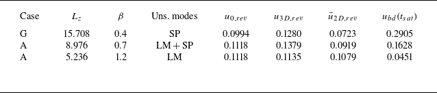
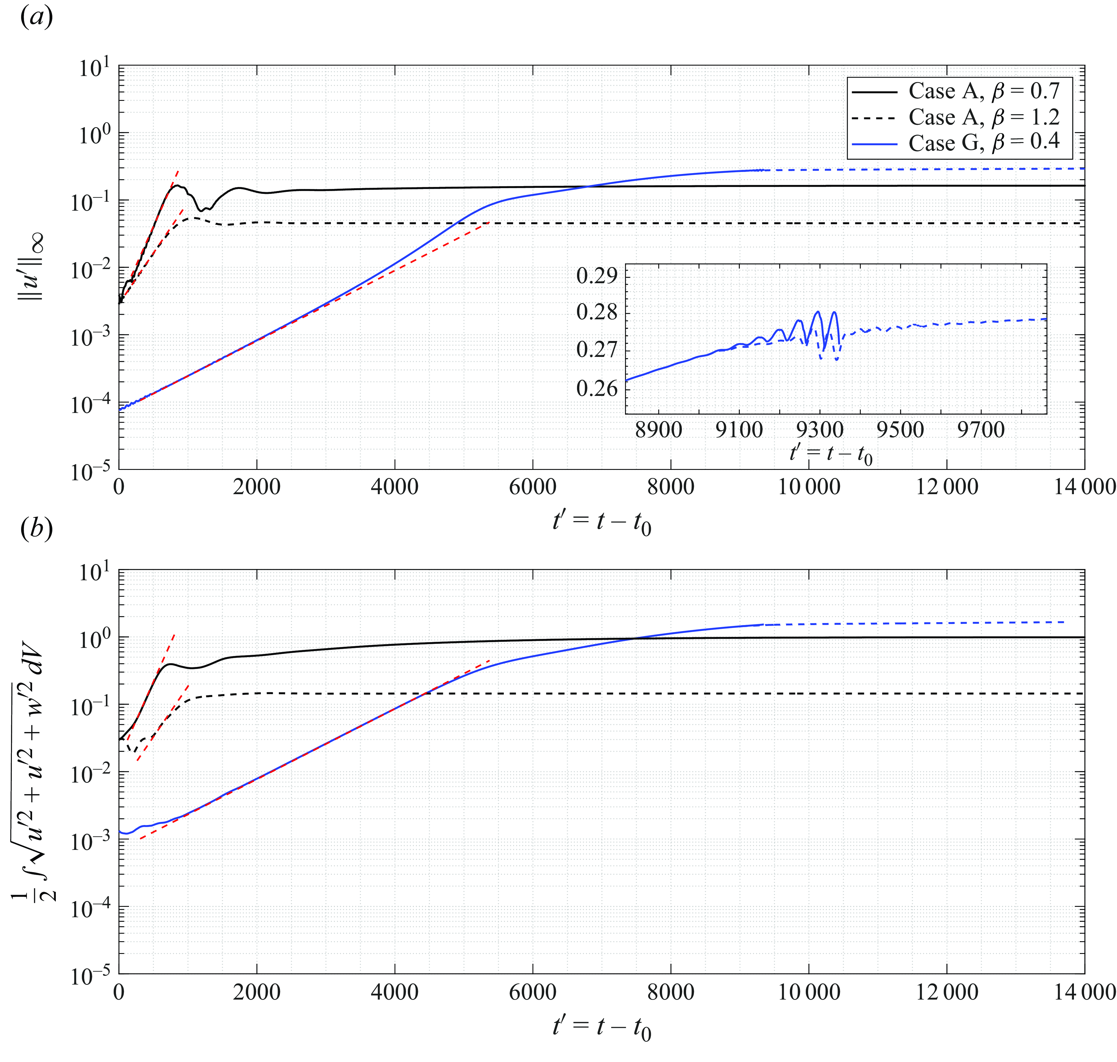
Figure 13. Time evolution of the peak of the absolute value of streamwise perturbation ( $\|u'\|_{\infty }$
) (a) and integrated kinetic energy of perturbations (b) for case A with
$\|u'\|_{\infty }$
) (a) and integrated kinetic energy of perturbations (b) for case A with $\beta =0.7$
(solid black line), case A with
$\beta =0.7$
(solid black line), case A with $\beta =1.2$
(dashed black line) and case G with
$\beta =1.2$
(dashed black line) and case G with $\beta =0.4$
(solid blue line). The blue dashed line correspond to case G after applying SFD. The inset in panel (a) shows the oscillations that happen for case G before using SFD. The red dashed lines show the growth rate predictions based on LST. Note that
$\beta =0.4$
(solid blue line). The blue dashed line correspond to case G after applying SFD. The inset in panel (a) shows the oscillations that happen for case G before using SFD. The red dashed lines show the growth rate predictions based on LST. Note that $t_0$
is the transient time that is different for each case. Note that the simulations are run for a much longer time than the part shown in this figure.
$t_0$
is the transient time that is different for each case. Note that the simulations are run for a much longer time than the part shown in this figure.
Figure 13(a) shows the temporal evolution of the absolute value of the peak streamwise perturbation component $\|u'\|_{\infty }$
for each case, where
$\|u'\|_{\infty }$
for each case, where ${u}'(x,y,z,t) = {u}_{3D}(x,y,z,t) - {u}_0(x,y)$
is the difference between the instantaneous velocity and the two-dimensional base flow. All the simulations present an initial transient that is not shown here. In what follows, the time
${u}'(x,y,z,t) = {u}_{3D}(x,y,z,t) - {u}_0(x,y)$
is the difference between the instantaneous velocity and the two-dimensional base flow. All the simulations present an initial transient that is not shown here. In what follows, the time $t' = t-t_0$
is considered, where
$t' = t-t_0$
is considered, where $t_0$
is an arbitrary time after the initial transient but before important dynamics appears. The evolution of disturbance kinetic energy
$t_0$
is an arbitrary time after the initial transient but before important dynamics appears. The evolution of disturbance kinetic energy $E(t) = \sqrt {(\boldsymbol{u}' \cdot \boldsymbol{u}')}/2$
is shown in figure 13(b). Note that the energy is integrated in the whole domain. The instantaneous growth rate of the disturbances can be computed from the DNS data using the disturbance energy as
$E(t) = \sqrt {(\boldsymbol{u}' \cdot \boldsymbol{u}')}/2$
is shown in figure 13(b). Note that the energy is integrated in the whole domain. The instantaneous growth rate of the disturbances can be computed from the DNS data using the disturbance energy as
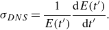 \begin{equation} \sigma _{DNS} = \frac {1}{E(t')}\frac {{\rm d}E(t')}{{\rm d}t'}. \end{equation}
In figure 13 the red dashed lines show the growth of the most unstable mode for each case obtained from linear theory (figure 10). In the following, an overview of the nonlinear saturation process for each of these three cases will be given.
-
(i) Case G, $\beta =0.4$
: this case aims to investigate the dynamics when only a single spread mode is present. The perturbation experiences an exponential growth for a long time (at
$t'\approx 3300$
,
$\sigma _{DNS}\approx 0.001200$
and
$\sigma _{LST}\approx 0.001204$
) followed by a slower growth due to nonlinear interactions of higher harmonics of the spanwise wavelength starting from
$t'=(t-t_0) \approx 5000$
, as is clear from the reduced slope of the blue line in figure 13(b). At
$t' \approx 9000$
, oscillations starts to appear in the shear layer close to reattachment point, as shown in the inset of figure 13(a). These oscillations are an indicator of a self-excited secondary instability that could lead to transition (Rodríguez et al. Reference Rodríguez, Gennaro and Souza2021a
). Note that, figure 13(a) shows the time evolution of the peak of the absolute value of
$u'$
in the whole domain, i.e.
$\|u'\|_{\infty }$
. Thus, the slope of amplitude growths in figure13(a) should not be considered as the growth rate of perturbations, since the point corresponding to peak perturbation might vary over time. However, this figure is useful to identify self-excited oscillations in the domain when the kinetic energy of the domain is not a good metric (since the oscillations do not appear in such an integral metric), and the location of oscillations is not known a priori. The subsequent transition process will be investigated in § 6. Here, to obtain the saturated base flow for this case for further analysis, when oscillations start to appear in the flow, SFD is activated. The saturated base flow is assumed to be converged when no significant change up to the seventh digit was found in
$\| u' \|_\infty$
. The blue dashed line in figures 13(a) and 13((b) shows the evolution of
$\|u'\|_{\infty }$
and kinetic energy after activating the SFD.
$\beta =0.4$
: this case aims to investigate the dynamics when only a single spread mode is present. The perturbation experiences an exponential growth for a long time (at
$t'\approx 3300$
,
$\sigma _{DNS}\approx 0.001200$
and
$\sigma _{LST}\approx 0.001204$
) followed by a slower growth due to nonlinear interactions of higher harmonics of the spanwise wavelength starting from
$t'=(t-t_0) \approx 5000$
, as is clear from the reduced slope of the blue line in figure 13(b). At
$t' \approx 9000$
, oscillations starts to appear in the shear layer close to reattachment point, as shown in the inset of figure 13(a). These oscillations are an indicator of a self-excited secondary instability that could lead to transition (Rodríguez et al. Reference Rodríguez, Gennaro and Souza2021a
). Note that, figure 13(a) shows the time evolution of the peak of the absolute value of
$u'$
in the whole domain, i.e.
$\|u'\|_{\infty }$
. Thus, the slope of amplitude growths in figure13(a) should not be considered as the growth rate of perturbations, since the point corresponding to peak perturbation might vary over time. However, this figure is useful to identify self-excited oscillations in the domain when the kinetic energy of the domain is not a good metric (since the oscillations do not appear in such an integral metric), and the location of oscillations is not known a priori. The subsequent transition process will be investigated in § 6. Here, to obtain the saturated base flow for this case for further analysis, when oscillations start to appear in the flow, SFD is activated. The saturated base flow is assumed to be converged when no significant change up to the seventh digit was found in
$\| u' \|_\infty$
. The blue dashed line in figures 13(a) and 13((b) shows the evolution of
$\|u'\|_{\infty }$
and kinetic energy after activating the SFD. -
(ii) Case A,
$\beta =1.2$
: this case aims to investigate the dynamics when only a single localised mode is present. The black dashed line in figure 13 shows that, after the initial transient, perturbations grow exponentially in the domain until nonlinear saturation gives rise to a steady flow. As opposed to the previous case, new fluctuations do not appear after the saturation. The growth rate of the exponential growth phase is approximated at
$t' \approx 550$
. For this case,
$\sigma _{DNS} \approx 0.003473$
which is close to that obtained using linear stability analysis,
$\sigma _{LST}=0.003488$
. -
(iii) Case A,
$\beta =0.7$
: in this case, the localised mode and its first harmonic (
$\beta =1.4$
) coexist with an unstable spread mode with
$\beta = 0.7$
. The same scenario as in the previous case is recovered. However, the growth rate of perturbations is larger than that for
$\beta =1.2$
, as figure 10 also suggests. Surprisingly, for this case, the saturated state is achieved for later times compared with
$\beta =1.2$
. The reason for this is that the rapid initial exponential growth shown in figure 13 (at
$t'_0 \approx 300$
,
$\sigma _{DNS}=0.0.005320$
and
$\sigma _{LST}=0.005439$
) is due to the localised mode. However, the spread mode that is also unstable keeps growing with a growth rate much lower than that of the localised mode. Nevertheless, a steady saturated state is obtained that again does not present signs of subsequent oscillations.


Table 4 summarises the maximum reverse flow for spanwise-homogeneous base flow ( $u_{0,rev}$
), spanwise averaged saturated base flow (
$u_{0,rev}$
), spanwise averaged saturated base flow ( $\bar {u}_{2D,rev}$
) and three-dimensional saturated base flow (
$\bar {u}_{2D,rev}$
) and three-dimensional saturated base flow ( $u_{3D,rev}$
), for the three cases considered here. The difference between
$u_{3D,rev}$
), for the three cases considered here. The difference between $u_{0,rev}$
and
$u_{0,rev}$
and $\bar {u}_{2D,rev}$
is an indicator of the magnitude of the mean flow distortion due to spanwise modulation of the initially two-dimensional base flow. In all three cases,
$\bar {u}_{2D,rev}$
is an indicator of the magnitude of the mean flow distortion due to spanwise modulation of the initially two-dimensional base flow. In all three cases, $u_{3D,rev}$
is larger and
$u_{3D,rev}$
is larger and $\bar {u}_{2D,rev}$
is smaller than
$\bar {u}_{2D,rev}$
is smaller than $u_{0,rev}$
. However, for case A with
$u_{0,rev}$
. However, for case A with $\beta =1.2$
, where only the localised unstable mode is present, the bubble experiences a weak mean flow distortion as the difference between peak reverse flows is very small. Case G, despite the comparatively lower growth rate of its eigenmode, presents the largest peak mean flow distortion.
$\beta =1.2$
, where only the localised unstable mode is present, the bubble experiences a weak mean flow distortion as the difference between peak reverse flows is very small. Case G, despite the comparatively lower growth rate of its eigenmode, presents the largest peak mean flow distortion.
4.2.2. Base flow distortion induced by the three-dimensional instability
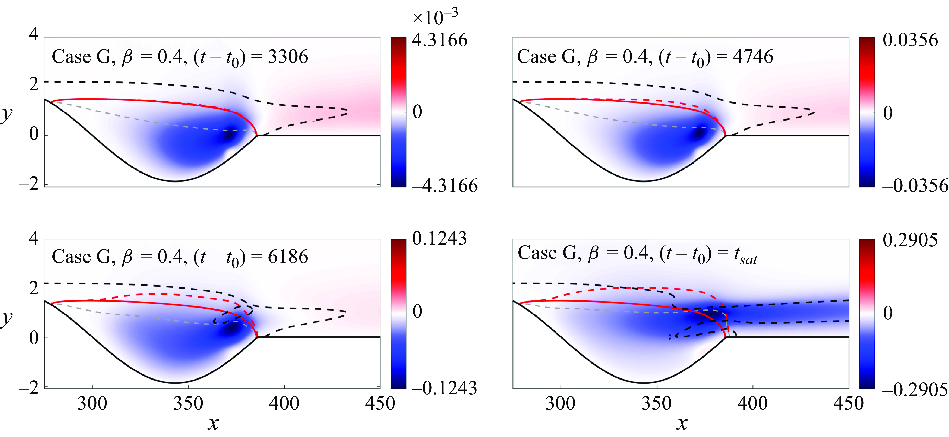
Figure 14. Contours of the base flow distortion $u_{bd}$
for case G (
$u_{bd}$
for case G ( $\beta =0.4$
) at four different times. The streamwise planes are plotted at the spanwise location with a peak negative base flow distortion value. The red solid and dashed lines show the location of the dividing streamline for the initial two-dimensional base flow and instantaneous flow, respectively. The dashed black line shows the location of the streamwise inflection point. The thin grey dashed line shows the location of the reverse flow streamline. The colour bars are symmetric and the negative limit at each panel shows the peak negative base flow distortion value at the corresponding time. The figure is not drawn to scale.
$\beta =0.4$
) at four different times. The streamwise planes are plotted at the spanwise location with a peak negative base flow distortion value. The red solid and dashed lines show the location of the dividing streamline for the initial two-dimensional base flow and instantaneous flow, respectively. The dashed black line shows the location of the streamwise inflection point. The thin grey dashed line shows the location of the reverse flow streamline. The colour bars are symmetric and the negative limit at each panel shows the peak negative base flow distortion value at the corresponding time. The figure is not drawn to scale.
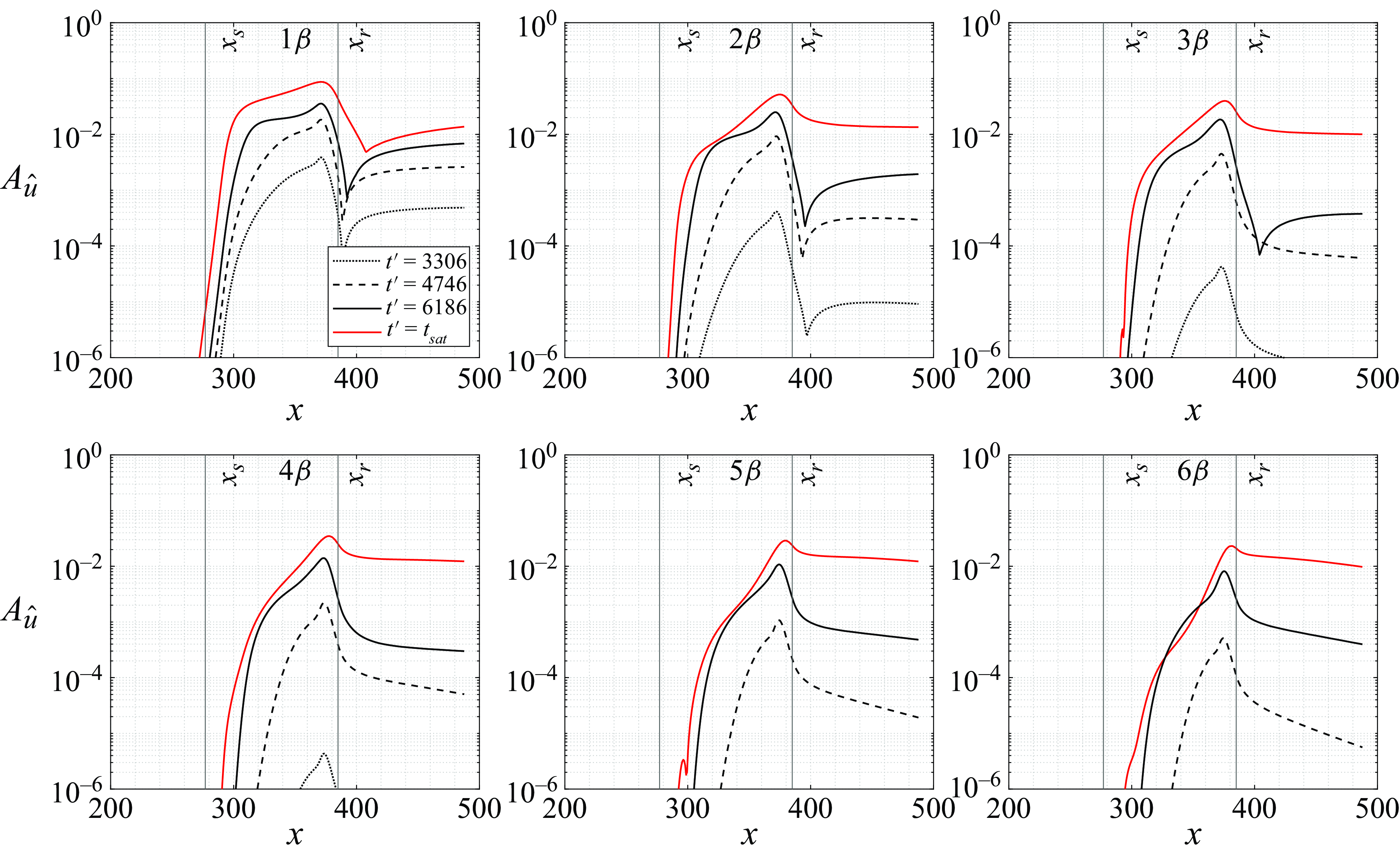
Figure 15. Spatial evolution of amplitudes of individual spanwise harmonics modes ( $A_{\hat {u}}$
) for case G at four time instances shown in figure 14. The separation and reattachment points are marked by vertical lines with labels
$A_{\hat {u}}$
) for case G at four time instances shown in figure 14. The separation and reattachment points are marked by vertical lines with labels $x_s$
and
$x_s$
and $x_r$
, respectively. The amplitude of the fundamental mode (
$x_r$
, respectively. The amplitude of the fundamental mode ( $1\beta$
) and first five harmonics (
$1\beta$
) and first five harmonics ( $2\beta -6\beta$
) are shown in the figure.
$2\beta -6\beta$
) are shown in the figure.
The nonlinear simulations discussed in the previous section recover steady saturated flows, either because of the absence of spontaneously growing oscillations or because SFD is used to damp the oscillations. In consequence, the simulated disturbance field $\boldsymbol{u}'(x,y,z,t)$
corresponds to the nonlinear distortion of the two-dimensional base flow
$\boldsymbol{u}'(x,y,z,t)$
corresponds to the nonlinear distortion of the two-dimensional base flow $\boldsymbol{u}_0$
induced by the three-dimensional instability. To remark this and distinguish it from the disturbance fields appearing in the simulations in later sections, the base flow distortion will be referred to as
$\boldsymbol{u}_0$
induced by the three-dimensional instability. To remark this and distinguish it from the disturbance fields appearing in the simulations in later sections, the base flow distortion will be referred to as $\boldsymbol{u}_{bd}(x,y,z,t)= \boldsymbol{u}_{3D}(x,y,z,t) - \boldsymbol{u}_0(x,y)$
. Note that the base flow distortion evolves in time until the final saturated state is reached at time
$\boldsymbol{u}_{bd}(x,y,z,t)= \boldsymbol{u}_{3D}(x,y,z,t) - \boldsymbol{u}_0(x,y)$
. Note that the base flow distortion evolves in time until the final saturated state is reached at time $t'=t'_{sat}$
, which is different for each case. Figures 14, 16 and 17 show the evolution of the base flow distortion for the cases in table 4. The streamwise velocity field is shown at the spanwise location where the base flow distortion at
$t'=t'_{sat}$
, which is different for each case. Figures 14, 16 and 17 show the evolution of the base flow distortion for the cases in table 4. The streamwise velocity field is shown at the spanwise location where the base flow distortion at $t'=t'_{sat}$
has its peak negative value. In the plots, the dividing streamline for
$t'=t'_{sat}$
has its peak negative value. In the plots, the dividing streamline for $u_0$
, the section of the dividing streamsurface for
$u_0$
, the section of the dividing streamsurface for $u'$
and time
$u'$
and time $t'$
, the in-plane streamwise inflection points (
$t'$
, the in-plane streamwise inflection points ( $\partial ^2 u / \partial y^2=0)$
and the section of the
$\partial ^2 u / \partial y^2=0)$
and the section of the $u'= 0$
surface are also shown. Table 4 summarises the peak negative base flow distortion at the saturated state for the three cases considered here.
$u'= 0$
surface are also shown. Table 4 summarises the peak negative base flow distortion at the saturated state for the three cases considered here.
-
(i) Case G,
$\beta =0.4$
(figure 14). At
$t'=3306$
, the perturbations are still experiencing exponential growth (figure 13
b) and the base flow distortion is very similar to the global mode as expected. At
$t'=4746$
, the nonlinear interactions start to become visible as the change in slope of the blue curve in figure 13(b) shows and, as a result, the bubble starts to deform. At
$t'=6186$
, nonlinear interactions have further distorted the bubble and moved the location of the peak negative
$u_{bd}$
away from the wall. Finally, at saturation (
$t'_{sat} \approx 55\,000$
) the bubble is distorted completely and nonlinear interactions around the reattachment point introduce flow deformations that extend downstream of the bubble. At saturation, the line of external inflection points intersects the dividing streamline at
$x\approx 334$
. Avanci et al. (Reference Avanci, Rodríguez and Alves2019) showed that, under the parallel flow assumption, this is a necessary condition for absolute instability of Kelvin–Helmholtz instability and self-excited oscillations. Note that downstream of the reattachment point, based on the shape of the global mode, the base flow distortion should be positive in the plane where the base flow distortion inside the bubble is negative. However, from the figure it can be seen that the bubble has a strong distortion in the vicinity of the reattachment point, and negative base flow distortion appears even further downstream. Thus, it can be conjectured that the strong deformation of the bubble, and also the negative base flow distortion downstream of the reattachment point, is mainly due to nonlinearities resulting from the growth of the spread mode.Further evidence is shown in figure 15, which illustrates the nonlinear growth of harmonics of the wavenumber corresponding to the unstable eigenmode. First, the spanwise Fourier decomposition of the streamwise perturbation velocity is obtained, i.e.
(4.2)where
\begin{equation} u'=\sum _{n=0}^{N}\hat {u} \exp {(in \beta z)+\textrm{c.c.},} \end{equation}
$\beta$
is the fundamental spanwise wavenumber of the simulation domain. The amplitude of the individual spanwise harmonic mode is then defined at each streamwise coordinate
$x$
as(4.3)Figure 15 shows the amplitudes of the fundamental (
\begin{equation} A_{\hat {u}}(x)=\max \limits _{y} |\hat {u}(x,y)|. \end{equation}
$\beta$
) and first five harmonics (
$2\beta -6\beta$
) for the same time instances as in figure 14. While the amplitudes of the harmonics at the earlier times are nearly negligible, they grow over time showing a progressive transfer of energy from lower to higher harmonics and their eventual saturation at comparable amplitudes. Interestingly, the harmonics present their peak amplitudes in the vicinity of the reattachment point, explaining the localised changes during saturation observed in figure 14.
-
(ii) Case A,
$\beta =1.2$
(figure 16). At
$t'=500$
, the perturbations are still in their linear regime. Note that, as figure 12 also shows, the components of the global eigenmodes, unlike for the spread mode, vanish along the shear layer, except in a small region in the vicinity of the location where the global mode is maximum. For this reason, even at saturation, the bubble does not experience noticeable modulation and expansion except for a very weak distortion around
$x \approx 360$
where the localised mode is present, and also upstream due to nonlinear interactions. This also explains the weak mean flow distortion shown in table 4 for this case. An important feature of the saturated base flow when only the localised mode is present happens in the vicinity of the reattachment point, where the
$u$
component of the global eigenmode changes sign (figure 12). This is consistent with the base flow distortion observed at all times. As a result, in the vicinity of reattachment for this case, nonlinear interactions are in favour of increasing the streamwise velocity perturbations and cancelling the negative base flow distortion. Thus, negative-velocity base flow distortion does not happen outside of the base flow’s recirculating region and the bubble does not expand. Unlike for case G, the dividing streamline is practically unaltered.Figure 16. Contours of base flow distortion
$u_{bd}$
for case A (
$\beta =1.2$
) at four different times. The annotations are the same as for figure 14.Figure 17. Contours of base flow distortion
$u_{bd}$
for case A (
$\beta =0.7$
) at four different time instances. The annotations are the same as for figure 14. -
(iii) Case A,
$\beta =0.7$
(figure 17). In this case, two unstable eigenmodes coexist. Initially (e.g.
$t'=300$
), only the growth of the localised mode can be observed. No noticeable change in the dividing streamline is visible for this time. At
$t'=600$
, nonlinear interactions start to become relevant as the dividing streamline is deformed in the vicinity of the localised mode. Until this time, no sign of growth of the spread mode is visible. However, after
$t' \approx 2000$
, the spread mode becomes visible as shown by the base flow distortion at
$t'=2640$
; the base flow distortion resembles
$u_{bd}(t'=6186)$
for case G. The interaction of the two unstable modes shows itself near the reattachment point. It was shown for case G that the nonlinearities following the growth of the spread mode distorts the bubble, especially near the reattachment point, pushing the peak reversed flow region away from the wall. On the other hand, in the vicinity of the reattachment point, nonlinearities following the localised mode intensify the positive base flow distortion and prevent the bubble from getting distorted near the reattachment point. Here, the interaction of these two modes is such that the bubble deforms slightly at the reattachment point, but still the distortion is much weaker than in case G. One explanation can be that the growth rate of the localised mode is almost one order of magnitude higher than the growth of the spread mode and, in consequence, the nonlinearities due to rapid growth of the localised mode prevent the slower-growing spread mode from distorting the flow effectively near the reattachment point. In summary, the base flow distortion in this case results from the combined effects of spread and localised modes: the rapid growth of the localised mode suppresses bubble deformation near the reattachment point, while the slower growth of the spread mode causes the bubble to expand upstream of the reattachment point.


Figure 18 shows the base flow distortion in the $z$
–
$z$
– $y$
cross-stream plane at the streamwise location of the peak negative base flow distortion for three cases, together with the sections of the dividing streamsurface, the reverse flow surface and the local surface of inflection points, following the same convention as in figures 14, 16 and 17. The spanwise modulation of the bubbles is clear from this plot, showing that case G experiences the most intense spanwise modulation, while case A with
$y$
cross-stream plane at the streamwise location of the peak negative base flow distortion for three cases, together with the sections of the dividing streamsurface, the reverse flow surface and the local surface of inflection points, following the same convention as in figures 14, 16 and 17. The spanwise modulation of the bubbles is clear from this plot, showing that case G experiences the most intense spanwise modulation, while case A with $\beta =1.2$
is only slightly modulated. Interestingly, due to strong nonlinear interactions for case G, the reverse flow region becomes very localised in the spanwise direction, which explains the large value of negative base flow distortion for this case compared with other cases, as given in the last column of table 4.
$\beta =1.2$
is only slightly modulated. Interestingly, due to strong nonlinear interactions for case G, the reverse flow region becomes very localised in the spanwise direction, which explains the large value of negative base flow distortion for this case compared with other cases, as given in the last column of table 4.
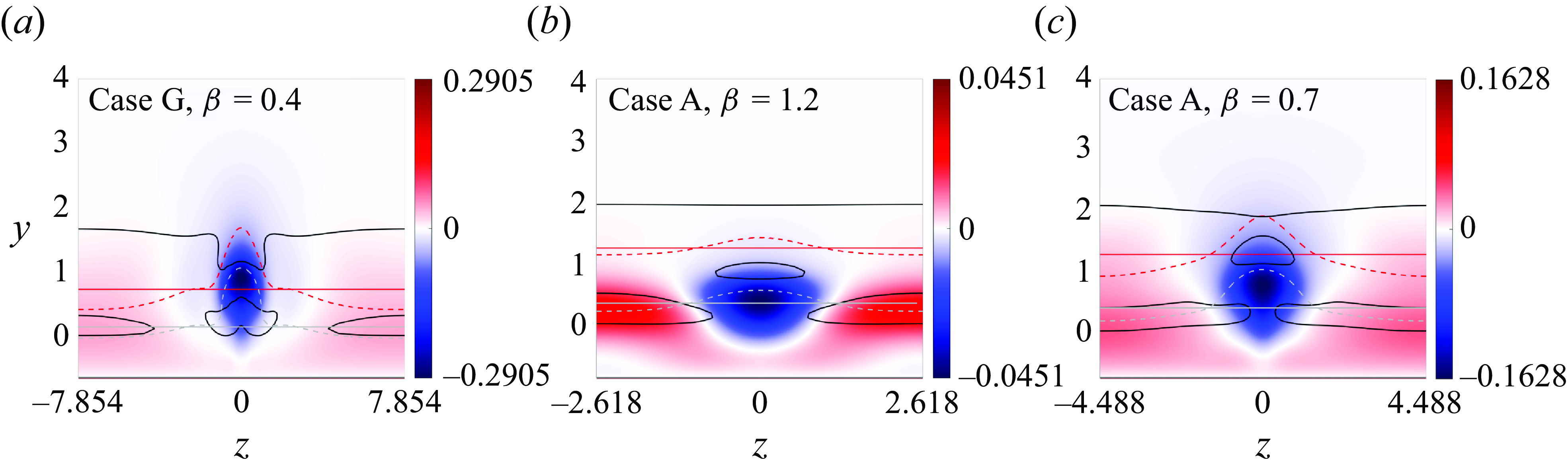
Figure 18. Contours of the base flow distortion in the $z$
–
$z$
– $y$
plane for
$y$
plane for $(a)$
case G (
$(a)$
case G ( $\beta =0.4$
) at
$\beta =0.4$
) at $x\approx 378$
,
$x\approx 378$
, $(b)$
case A (
$(b)$
case A ( $\beta =1.2$
) at
$\beta =1.2$
) at $x\approx 363$
and (
$x\approx 363$
and ( $c$
) case A (
$c$
) case A ( $\beta =0.7$
) at
$\beta =0.7$
) at $x\approx 364$
. The annotations are the same as for figure 14. The thin grey solid line shows the location of the reverse flow streamline for the initially two-dimensional base flow.
$x\approx 364$
. The annotations are the same as for figure 14. The thin grey solid line shows the location of the reverse flow streamline for the initially two-dimensional base flow.
5. Self-excited oscillations developing on the saturated three-dimensional flow
Figure 13(a) showed that, for case G without using SFD, flow oscillations spontaneously appear. The same phenomena is observed for an LSB on a flat plate (Rodríguez et al. Reference Rodríguez, Gennaro and Souza2021a ), where it was shown that the oscillations were caused by a secondary instability of the saturated flow. In this section the stability of the saturated flow is investigated first by solving the pertinent three-dimensional eigenvalue problem. Then, the linear response of the system to an impulse perturbation field is investigated.
5.1. Secondary global stability analysis
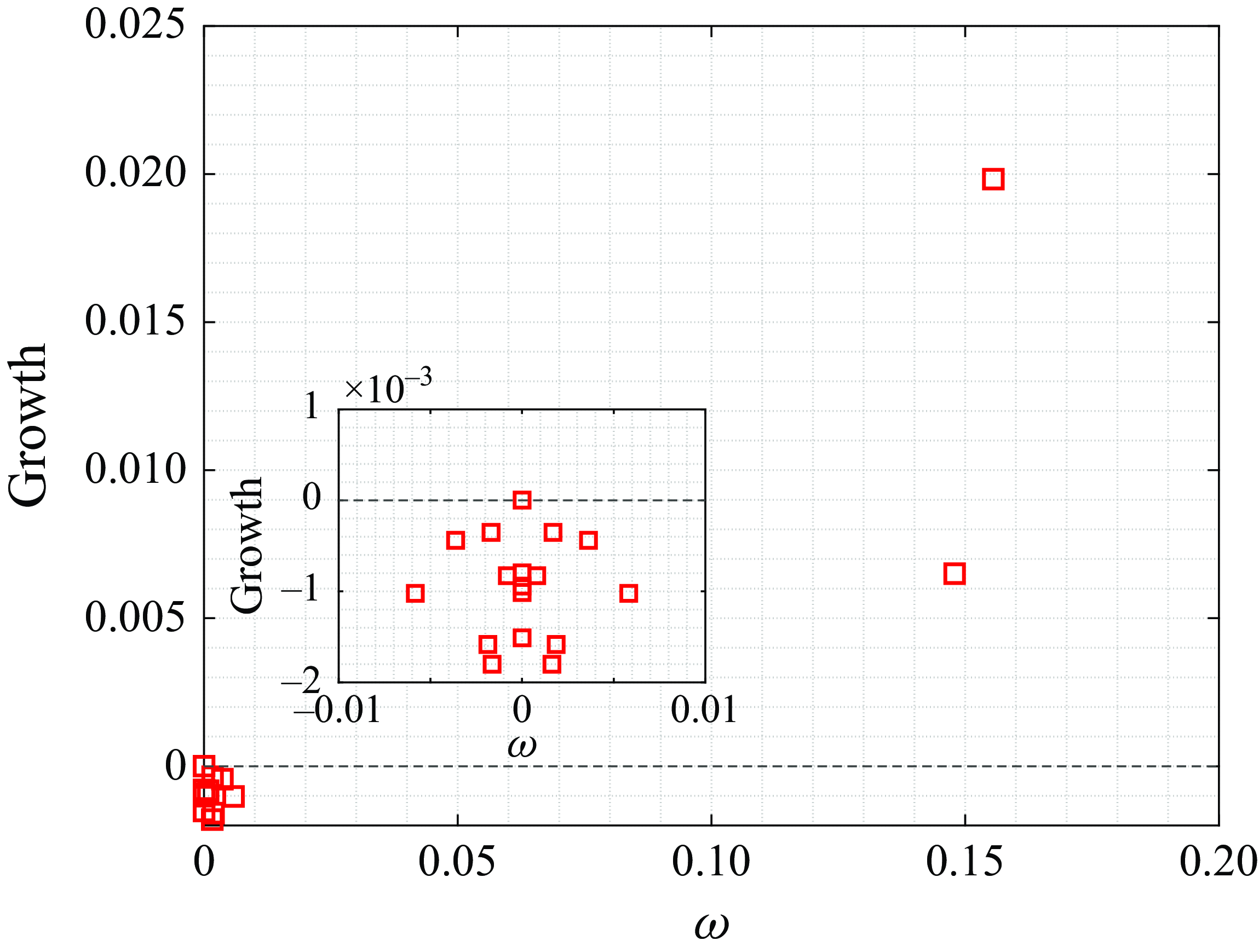
Figure 19. Secondary eigenvalue spectrum corresponding to the saturated flow for case G with $\beta =0.4$
. The inset shows the spectrum close to the origin.
$\beta =0.4$
. The inset shows the spectrum close to the origin.
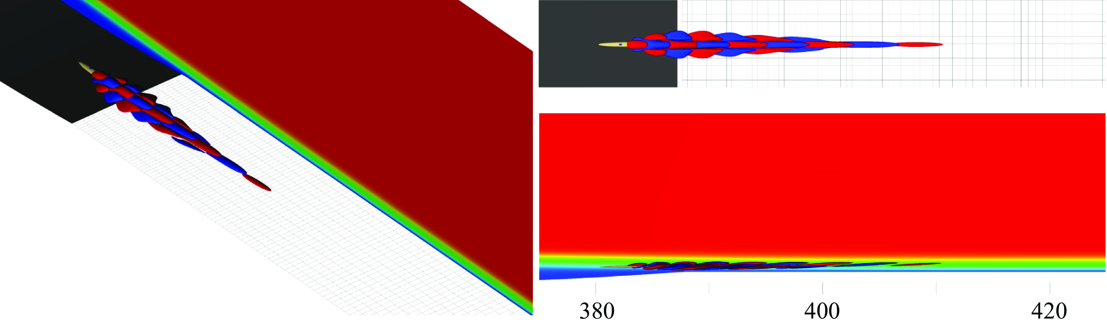
Figure 20. Real part of the $u$
component of the most unstable eigenmode corresponding to the saturated
$u$
component of the most unstable eigenmode corresponding to the saturated $\boldsymbol{u}_{3D}$
for case G with
$\boldsymbol{u}_{3D}$
for case G with $\beta =0.4$
. The yellow isosurface corresponds to
$\beta =0.4$
. The yellow isosurface corresponds to $u_{bd}=-0.25$
. The red and blue colours show the positive and negative values, respectively.
$u_{bd}=-0.25$
. The red and blue colours show the positive and negative values, respectively.
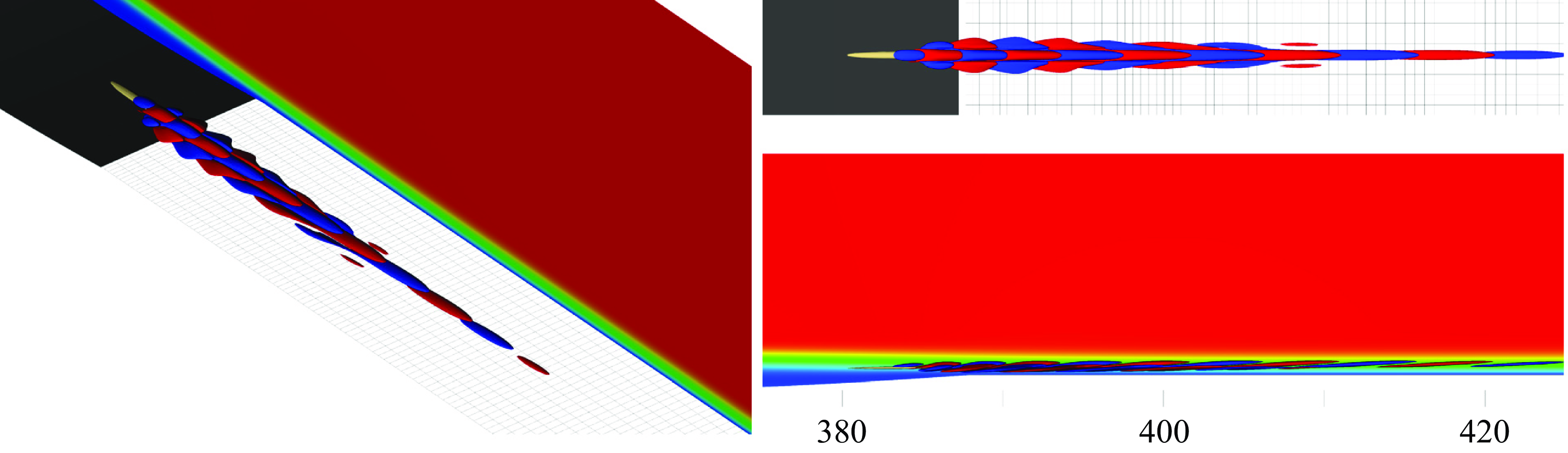
Figure 21. Same as figure 20 for the second most unstable eigenmode corresponding to the saturated $\boldsymbol{u}_{3D}$
for case G with
$\boldsymbol{u}_{3D}$
for case G with $\beta =0.4$
.
$\beta =0.4$
.
A three-dimensional global stability analysis of the saturated base flow $\boldsymbol{u}_{3D}$
for case G, which is obtained using SFD, is performed using the implicitly restarted Arnoldi method implemented in Nek5000. A Krylov subspace size of 100 is used to ensure convergence of at least the first 20 eigenvalues. The eigenspectra, shown in figure 19, contains two unstable modes with (
$\boldsymbol{u}_{3D}$
for case G, which is obtained using SFD, is performed using the implicitly restarted Arnoldi method implemented in Nek5000. A Krylov subspace size of 100 is used to ensure convergence of at least the first 20 eigenvalues. The eigenspectra, shown in figure 19, contains two unstable modes with ( $\omega, \sigma )=(0.1479,0.0065)$
and (
$\omega, \sigma )=(0.1479,0.0065)$
and ( $\omega, \sigma )=(0.1555,0.0198)$
. In the proximity of
$\omega, \sigma )=(0.1555,0.0198)$
. In the proximity of $\omega =0$
(the zoomed inset in the figure), a family of stable low-frequency modes appears. The shape and role of these modes in the dynamics is explained in § 6.1. The spatial structure of the
$\omega =0$
(the zoomed inset in the figure), a family of stable low-frequency modes appears. The shape and role of these modes in the dynamics is explained in § 6.1. The spatial structure of the $u$
component of the most unstable and second unstable modes are shown in figures 20 and 21, respectively. In these figures, the yellow isosurface corresponds to
$u$
component of the most unstable and second unstable modes are shown in figures 20 and 21, respectively. In these figures, the yellow isosurface corresponds to $u_{bd}=-0.25$
, i.e.
$u_{bd}=-0.25$
, i.e. $86 \,\%$
of the peak negative base flow distortion
$86 \,\%$
of the peak negative base flow distortion $u_{bd,min}$
. Both unstable modes are varicose (symmetric) on the spanwise direction and are rooted around the peak negative base flow distortion. Note that both the peak reverse flow and base flow distortion
$u_{bd,min}$
. Both unstable modes are varicose (symmetric) on the spanwise direction and are rooted around the peak negative base flow distortion. Note that both the peak reverse flow and base flow distortion $u_{bd,min}$
occur at the same spanwise plane; however, the location of
$u_{bd,min}$
occur at the same spanwise plane; however, the location of $u_{bd,min}$
,
$u_{bd,min}$
, $(x,y)_{bd}=(378.4,0.97)$
, is located slightly downstream and above the location of the peak negative reverse flow (
$(x,y)_{bd}=(378.4,0.97)$
, is located slightly downstream and above the location of the peak negative reverse flow ( $(x,y)_{rev}=(369.8,0.62)$
). The second unstable mode has a slightly longer wavelength compared with the most unstable one, and it has a larger downstream spatial extension. Using a weakly non-parallel Wentzel–Kramers–Brillouin–Jeffreys (WKBJ) analysis, Rodríguez et al. (Reference Rodríguez, Gennaro and Souza2021a
) approximated the properties of the most unstable eigenmode responsible for self-excited secondary instability in a pressure-gradient-induced LSB over a flat plate. The spatial structure of the eigenmode found in that work looks qualitatively similar to both eigenmodes found here using global stability analysis. Furthermore, the varicose eigenmodes here look similar to the eigenmodes found in the wake region of a cylindrical isolated roughness element with a diameter-to-height aspect ratio larger than one (Loiseau et al. Reference Loiseau, Robinet, Cherubini and Leriche2014), and also to those recovered for a cuboid isolated roughness element when the height of the roughness is large compared with the boundary layer displacement thickness (Ma & Mahesh Reference Ma and Mahesh2022). It is anticipated here that these eigenmodes will give rise to self-excited oscillations in the rear part of the bubble, in the vicinity of
$(x,y)_{rev}=(369.8,0.62)$
). The second unstable mode has a slightly longer wavelength compared with the most unstable one, and it has a larger downstream spatial extension. Using a weakly non-parallel Wentzel–Kramers–Brillouin–Jeffreys (WKBJ) analysis, Rodríguez et al. (Reference Rodríguez, Gennaro and Souza2021a
) approximated the properties of the most unstable eigenmode responsible for self-excited secondary instability in a pressure-gradient-induced LSB over a flat plate. The spatial structure of the eigenmode found in that work looks qualitatively similar to both eigenmodes found here using global stability analysis. Furthermore, the varicose eigenmodes here look similar to the eigenmodes found in the wake region of a cylindrical isolated roughness element with a diameter-to-height aspect ratio larger than one (Loiseau et al. Reference Loiseau, Robinet, Cherubini and Leriche2014), and also to those recovered for a cuboid isolated roughness element when the height of the roughness is large compared with the boundary layer displacement thickness (Ma & Mahesh Reference Ma and Mahesh2022). It is anticipated here that these eigenmodes will give rise to self-excited oscillations in the rear part of the bubble, in the vicinity of $u_{bd,min}$
, and will cause a rapid transition to turbulence. The transition process is investigated in detail in § 6.1.
$u_{bd,min}$
, and will cause a rapid transition to turbulence. The transition process is investigated in detail in § 6.1.
5.2. Impulse response analysis
To investigate the linear response of the saturated flow $\boldsymbol{u}_{3D}$
to perturbations, a linear simulation is performed in which a spatially localised initial disturbance is introduced at
$\boldsymbol{u}_{3D}$
to perturbations, a linear simulation is performed in which a spatially localised initial disturbance is introduced at $x\approx 370$
, close to the location of the peak reversed flow. The spatial structure of the initial disturbance is described in Appendix B.
$x\approx 370$
, close to the location of the peak reversed flow. The spatial structure of the initial disturbance is described in Appendix B.
The solid black line in figure 22 shows the evolution of the disturbance kinetic energy $E$
and the red dashed line shows the growth rate of the most unstable eigenmode calculated using global stability analysis confirming that, after an initial transient growth, the linear disturbance is governed by the most unstable eigenmode. Due to the large gap between the growth rates of the two unstable modes, the most unstable mode becomes dominant very quickly. As a result, a beating phenomena at the frequency difference between those of the two unstable modes, as that recovered by, for example, Ehrenstein & Gallaire (Reference Ehrenstein and Gallaire2008), does not happen here. Instead, an exponential disturbance growth in which the disturbance field (figure 20) and the oscillation frequency closely follow the prediction of the global stability analysis is recovered and it continues until nonlinearities set in.
$E$
and the red dashed line shows the growth rate of the most unstable eigenmode calculated using global stability analysis confirming that, after an initial transient growth, the linear disturbance is governed by the most unstable eigenmode. Due to the large gap between the growth rates of the two unstable modes, the most unstable mode becomes dominant very quickly. As a result, a beating phenomena at the frequency difference between those of the two unstable modes, as that recovered by, for example, Ehrenstein & Gallaire (Reference Ehrenstein and Gallaire2008), does not happen here. Instead, an exponential disturbance growth in which the disturbance field (figure 20) and the oscillation frequency closely follow the prediction of the global stability analysis is recovered and it continues until nonlinearities set in.
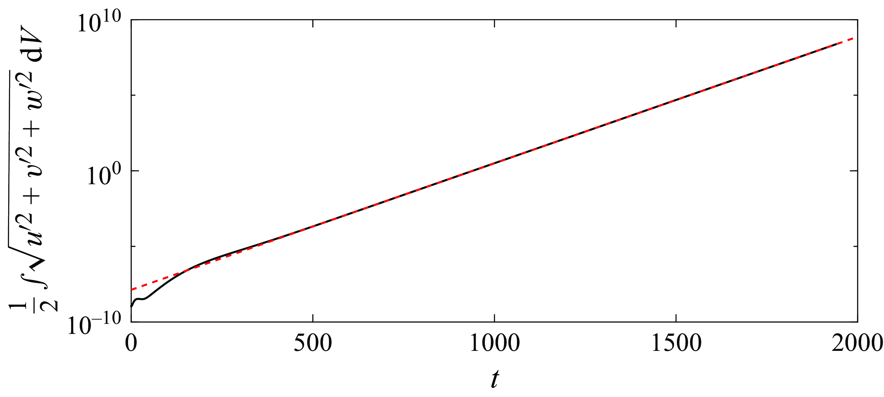
Figure 22. The time evolution of the perturbation energy (solid black line) as a result of an impulse perturbation field imposed at $t=0$
, considering the saturated flow
$t=0$
, considering the saturated flow $\boldsymbol{u}_{3D}$
for case G with
$\boldsymbol{u}_{3D}$
for case G with $\beta =0.4$
as the base flow. The red dashed line shows the growth rate of the most unstable eigenmode in figure 19.
$\beta =0.4$
as the base flow. The red dashed line shows the growth rate of the most unstable eigenmode in figure 19.
6. Transition scenarios
In this section, transition to turbulence is investigated for two representative cases: case G with $\beta =0.4 {\, (L_z=2\pi /0.4})$
considered in the previous section and that presents a single three-dimensional unstable eigenmode, and case E with
$\beta =0.4 {\, (L_z=2\pi /0.4})$
considered in the previous section and that presents a single three-dimensional unstable eigenmode, and case E with $\beta =0.6{\, (L_z=2\pi /0.6)}$
, where the base flow is globally unstable with respect to both two- and three-dimensional instabilities. Note that,
$\beta =0.6{\, (L_z=2\pi /0.6)}$
, where the base flow is globally unstable with respect to both two- and three-dimensional instabilities. Note that, $\beta =0.6$
corresponds to the spanwise wavenumber of the most unstable mode for case E (figure 10).
$\beta =0.6$
corresponds to the spanwise wavenumber of the most unstable mode for case E (figure 10).
6.1. Case G,
$\beta =0.4$

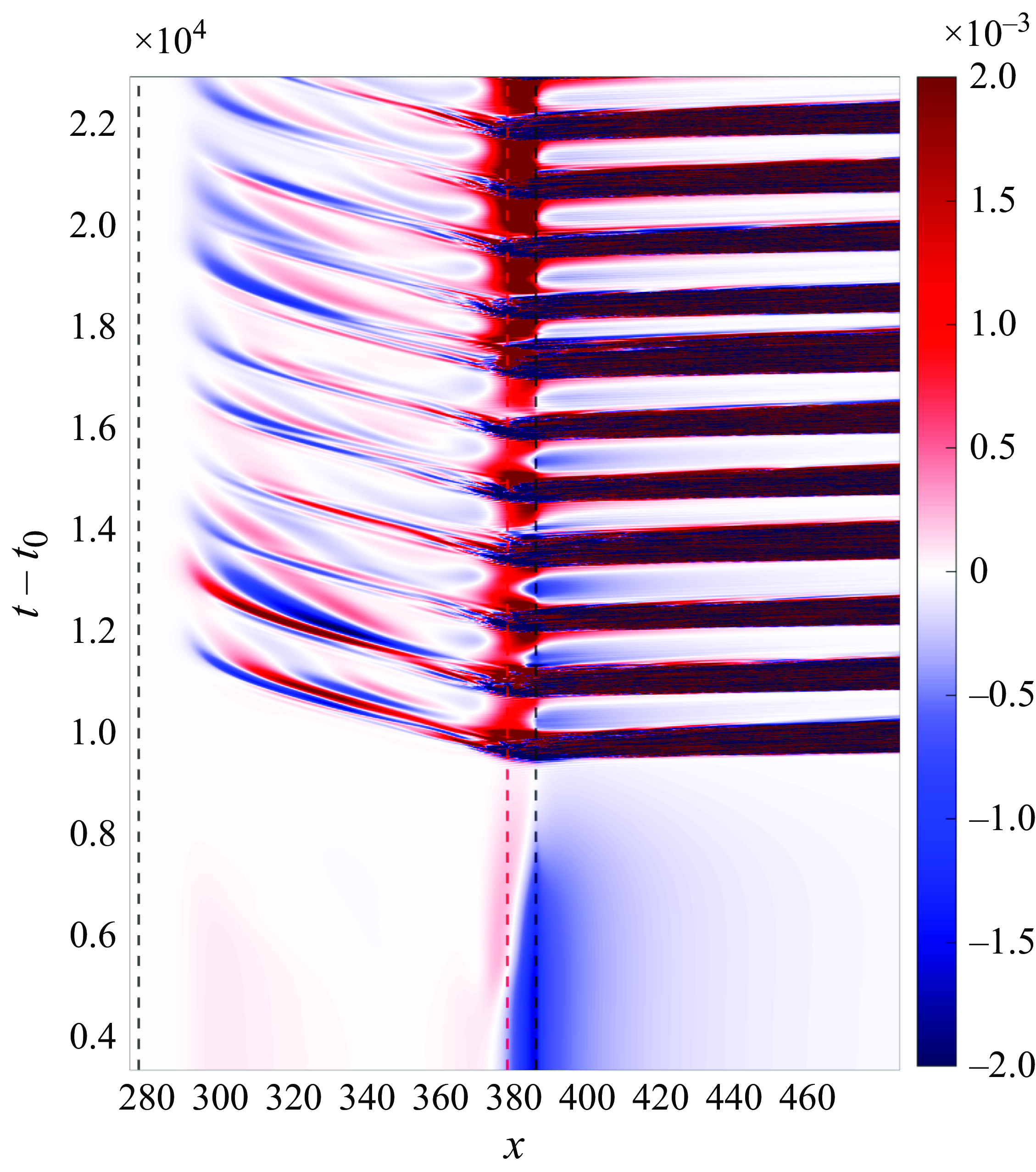
Figure 23. Spatio-temporal diagram of spanwise perturbation velocity for case G with $\beta =0.4$
, along a curve parallel to the wavy wall that passes through the location of
$\beta =0.4$
, along a curve parallel to the wavy wall that passes through the location of $u_{bd,min}$
. The dashed black lines show the location of the separation and reattachment point, and the red dashed line shows the location of peak negative base flow distortion. Note that the perturbations are calculated based on the saturated flow
$u_{bd,min}$
. The dashed black lines show the location of the separation and reattachment point, and the red dashed line shows the location of peak negative base flow distortion. Note that the perturbations are calculated based on the saturated flow $\boldsymbol{u}_{3D}$
.
$\boldsymbol{u}_{3D}$
.
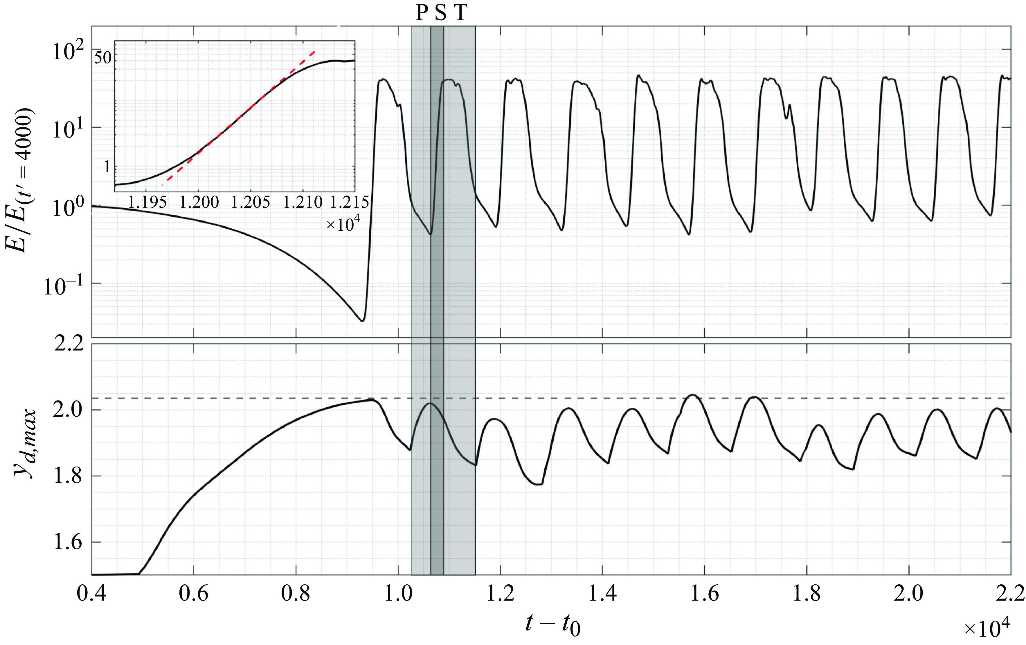
Figure 24. Top panel: the time evolution of the perturbation kinetic energy (calculated with respect to the saturated $\boldsymbol{u}_{3D}$
) for case G with
$\boldsymbol{u}_{3D}$
) for case G with $\beta =0.4$
. The inset zooms in on region ‘S’ corresponding to
$\beta =0.4$
. The inset zooms in on region ‘S’ corresponding to $11\,950\lt t'\lt 12\,150$
. Bottom panel: maximum
$11\,950\lt t'\lt 12\,150$
. Bottom panel: maximum $y$
coordinate of the dividing streamline in the streamwise plane with peak negative base flow distortion. The horizontal dashed line indicates the maximum
$y$
coordinate of the dividing streamline in the streamwise plane with peak negative base flow distortion. The horizontal dashed line indicates the maximum $y$
coordinate of the dividing streamline in the saturated state. The shaded areas indicate the P, S and T temporal phases for the second turbulent burst.
$y$
coordinate of the dividing streamline in the saturated state. The shaded areas indicate the P, S and T temporal phases for the second turbulent burst.
The simulation shown in figure 13 is continued without applying SFD after the appearance of self-excited oscillations at $t'\approx 9000$
. Note that the oscillations start to appear before the primary instability fully saturates and the peak negative base flow distortion (
$t'\approx 9000$
. Note that the oscillations start to appear before the primary instability fully saturates and the peak negative base flow distortion ( $u'_{bd,min}\approx 0.27$
) is slightly lower than its value at the fully saturated state that is used to perform the secondary stability analysis in § 5, namely
$u'_{bd,min}\approx 0.27$
) is slightly lower than its value at the fully saturated state that is used to perform the secondary stability analysis in § 5, namely $u'_{bd,min}\approx 0.29$
. Figure 23 shows the
$u'_{bd,min}\approx 0.29$
. Figure 23 shows the $x{-}t$
diagram for spanwise perturbation velocities for a line (
$x{-}t$
diagram for spanwise perturbation velocities for a line ( $x \in [275,485]$
) parallel and close to the wavy wall in the streamwise plane that passes through the location of the peak negative base flow distortion corresponding to the saturated state. The perturbation velocity here is calculated using the saturated flow
$x \in [275,485]$
) parallel and close to the wavy wall in the streamwise plane that passes through the location of the peak negative base flow distortion corresponding to the saturated state. The perturbation velocity here is calculated using the saturated flow $\boldsymbol{u}_{3D}$
as reference, not the two-dimensional initial base flow
$\boldsymbol{u}_{3D}$
as reference, not the two-dimensional initial base flow $\boldsymbol{u}_0$
. The spatio-temporal diagram shows two specific features of this flow. First, after the appearance of oscillations at
$\boldsymbol{u}_0$
. The spatio-temporal diagram shows two specific features of this flow. First, after the appearance of oscillations at $t' \approx 9000$
, breakdown to turbulence happens, starting around
$t' \approx 9000$
, breakdown to turbulence happens, starting around $x \approx 378$
. However, the flow undergoes a relaminarisation after that. This turbulent burst-relaminarisation cycle repeats itself subsequently, with an angular repetition frequency
$x \approx 378$
. However, the flow undergoes a relaminarisation after that. This turbulent burst-relaminarisation cycle repeats itself subsequently, with an angular repetition frequency $\omega \approx 0.0048-0.0057$
, estimated from figure 23. Second, after each turbulent burst, spanwise perturbations travel upstream within the bubble. In the following, each of these observations will be explained in detail.
$\omega \approx 0.0048-0.0057$
, estimated from figure 23. Second, after each turbulent burst, spanwise perturbations travel upstream within the bubble. In the following, each of these observations will be explained in detail.
6.1.1. Turbulent burst-relaminarisation cycle
The top panel in figure 24 shows the kinetic energy of the perturbations integrated in the domain for $280\lt x\lt 490$
(normalised by the energy at
$280\lt x\lt 490$
(normalised by the energy at $t'=4000$
). The bottom panel shows the maximum
$t'=4000$
). The bottom panel shows the maximum $y$
coordinate of the dividing streamline of the bubble in the spanwise plane with peak negative base flow distortion, which is an indicator of the instantaneous height of the bubble. Starting from
$y$
coordinate of the dividing streamline of the bubble in the spanwise plane with peak negative base flow distortion, which is an indicator of the instantaneous height of the bubble. Starting from $t'=4000$
, the height of the bubble increases slowly until
$t'=4000$
, the height of the bubble increases slowly until $t'\approx 4900$
, when the nonlinear interactions become relevant and induce a strong spanwise modulation of the bubble, as explained in § 4.2.2. Then, the height of the bubble keeps increasing, which results in a strong peak negative base flow distortion and triggers a self-excited secondary instability. Soon after the appearance of oscillations (figure 13), for
$t'\approx 4900$
, when the nonlinear interactions become relevant and induce a strong spanwise modulation of the bubble, as explained in § 4.2.2. Then, the height of the bubble keeps increasing, which results in a strong peak negative base flow distortion and triggers a self-excited secondary instability. Soon after the appearance of oscillations (figure 13), for $9300\lt t'\lt 9600$
, the secondary instabilities grow exponentially in the domain that cause the rapid increase of perturbation kinetic energy. Once the flow oscillations arising from the secondary instability reach nonlinear amplitudes, for
$9300\lt t'\lt 9600$
, the secondary instabilities grow exponentially in the domain that cause the rapid increase of perturbation kinetic energy. Once the flow oscillations arising from the secondary instability reach nonlinear amplitudes, for $9600\lt t'\lt 10\,000$
, a rapid transition to turbulence happens (which is also observable in figure 23). During this lapse of time, the vortical structures formed inside the bubble pull the fluid out of the bubble and cause the height of the bubble to decrease rapidly. Eventually, at
$9600\lt t'\lt 10\,000$
, a rapid transition to turbulence happens (which is also observable in figure 23). During this lapse of time, the vortical structures formed inside the bubble pull the fluid out of the bubble and cause the height of the bubble to decrease rapidly. Eventually, at $t' \approx 10\,000$
, the vortical structures leave the bubble and are advected downstream until they exit the computational domain. This is also visible in figure 23 where, at
$t' \approx 10\,000$
, the vortical structures leave the bubble and are advected downstream until they exit the computational domain. This is also visible in figure 23 where, at $t'\approx 10\,000$
, the leading edge of the spanwise perturbations is leaving the domain, causing a rapid decrease in perturbation energy. As a result, the bubble relaminarises and shrinks until it reaches an intermediate state with a minimum height (
$t'\approx 10\,000$
, the leading edge of the spanwise perturbations is leaving the domain, causing a rapid decrease in perturbation energy. As a result, the bubble relaminarises and shrinks until it reaches an intermediate state with a minimum height ( $t'=10\,200$
). Following from this initial turbulent burst, a cycle of spanwise deformation, secondary instability and turbulent burst is repeated in a quasi-periodic manner for the rest of the simulation.
$t'=10\,200$
). Following from this initial turbulent burst, a cycle of spanwise deformation, secondary instability and turbulent burst is repeated in a quasi-periodic manner for the rest of the simulation.
The shaded areas in figure 24 show three time lapses named P, S and T, which denote the main phases of the subsequent turbulent bursts. The regions are associated with primary (P) and secondary (S) instabilities, and the transition (T) region. After the first turbulent burst leaves the region adjacent to the wall waviness, the bubble reaches an intermediate state, at $t'\approx 10\,200$
, between its initial two-dimensional state and the saturated state where no secondary instability is active anymore; however, the primary instability is still globally unstable and drives the flow towards its saturated state again. This is clear from region P in figure 24, where the kinetic energy growth rate changes and the bubble height starts to increase until it reaches its maximum again. After that, in phase S, the negative base flow distortion is strong enough to trigger the secondary instabilities and the ensuing turbulent burst reoccurs in phase T.
$t'\approx 10\,200$
, between its initial two-dimensional state and the saturated state where no secondary instability is active anymore; however, the primary instability is still globally unstable and drives the flow towards its saturated state again. This is clear from region P in figure 24, where the kinetic energy growth rate changes and the bubble height starts to increase until it reaches its maximum again. After that, in phase S, the negative base flow distortion is strong enough to trigger the secondary instabilities and the ensuing turbulent burst reoccurs in phase T.
Recently, in an experiment of a pressure-gradient-induced LSB on a flat plate (Aniffa & Mandal Reference Aniffa and Mandal2023), a similar phenomenon was reported: a low-frequency oscillation of the shear layer and vertical motion of the inflection points that is accompanied by an intermittent vortex shedding where the bubble alternates between a non-vortex-shedding state and a shedding state. Here, it is also observed at $t'\approx 8400$
that the external streamwise inflection point crosses below the dividing streamsurface of the recirculation bubble. However, no sign of oscillations was observed until
$t'\approx 8400$
that the external streamwise inflection point crosses below the dividing streamsurface of the recirculation bubble. However, no sign of oscillations was observed until $t'\approx 9000$
, when the height of the bubble gets close to its maximum and the peak negative base flow distortion becomes strong enough to trigger the secondary instabilities. This is in agreement with the necessary condition for absolute instability of inflectional instability proposed by Avanci et al. (Reference Avanci, Rodríguez and Alves2019) and its three-dimensional analog seen in Rodríguez et al. (Reference Rodríguez, Gennaro and Souza2021a
).
$t'\approx 9000$
, when the height of the bubble gets close to its maximum and the peak negative base flow distortion becomes strong enough to trigger the secondary instabilities. This is in agreement with the necessary condition for absolute instability of inflectional instability proposed by Avanci et al. (Reference Avanci, Rodríguez and Alves2019) and its three-dimensional analog seen in Rodríguez et al. (Reference Rodríguez, Gennaro and Souza2021a
).
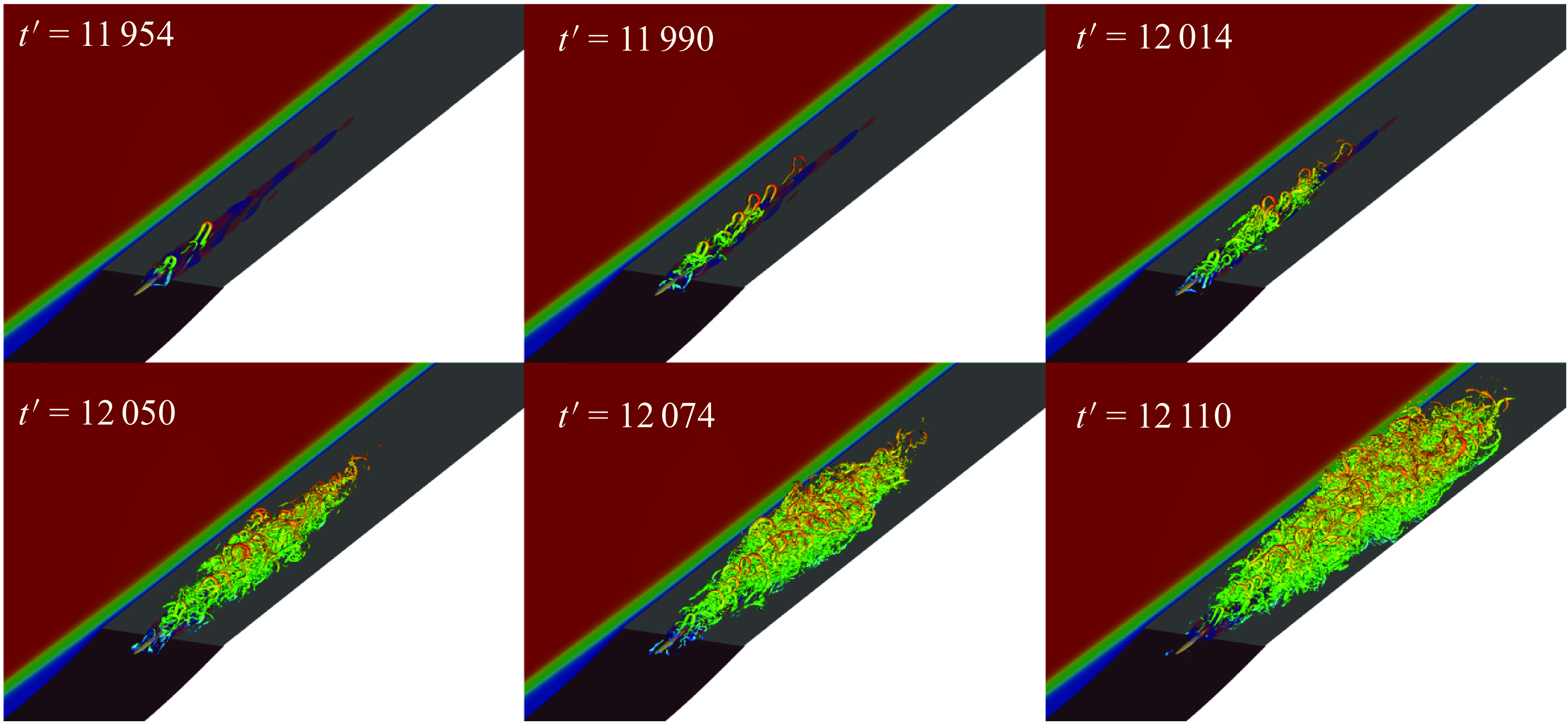
Figure 25. Instantaneous $\lambda _2$
visualizations (coloured by streamwise velocity) of the vortical structures in the flow for case G with
$\lambda _2$
visualizations (coloured by streamwise velocity) of the vortical structures in the flow for case G with $\beta = 0.4$
. The red (positive) and blue (negative) isosurfaces show the spatial structure of the second unstable global mode as shown in figure 21. The energy growth shown in the inset of figure 24 corresponds to the time interval shown in this figure. Note that different values of
$\beta = 0.4$
. The red (positive) and blue (negative) isosurfaces show the spatial structure of the second unstable global mode as shown in figure 21. The energy growth shown in the inset of figure 24 corresponds to the time interval shown in this figure. Note that different values of $\lambda _2$
are used in the different plots for better visualization.
$\lambda _2$
are used in the different plots for better visualization.
Figure 25 shows the vortical structures using $\lambda _2$
visualizations (Jeong & Hussain Reference Jeong and Hussain1995) coloured by streamwise velocity for six different time instants during
$\lambda _2$
visualizations (Jeong & Hussain Reference Jeong and Hussain1995) coloured by streamwise velocity for six different time instants during $11\,954\lt t'\lt 12\,110$
, corresponding to phase S before the third peak of disturbance energy in figure 24. The
$11\,954\lt t'\lt 12\,110$
, corresponding to phase S before the third peak of disturbance energy in figure 24. The $u$
component of the second unstable secondary instability (same as figure 21) is also shown. The inset in the top panel of figure 24 shows the growth of the disturbance energy for the same time span. Figures 24 and 25 show that, after the appearance of oscillations, a train of hairpin vortices starts to develop as a nonlinear consequence of the global eigenmode. The train of hairpin vortices here is similar to that reported downstream of a cylindrical roughness element by Loiseau et al. (Reference Loiseau, Robinet, Cherubini and Leriche2014), where the authors concluded that a varicose unstable global mode contributes to nonlinear generation of the hairpin vortices. From
$u$
component of the second unstable secondary instability (same as figure 21) is also shown. The inset in the top panel of figure 24 shows the growth of the disturbance energy for the same time span. Figures 24 and 25 show that, after the appearance of oscillations, a train of hairpin vortices starts to develop as a nonlinear consequence of the global eigenmode. The train of hairpin vortices here is similar to that reported downstream of a cylindrical roughness element by Loiseau et al. (Reference Loiseau, Robinet, Cherubini and Leriche2014), where the authors concluded that a varicose unstable global mode contributes to nonlinear generation of the hairpin vortices. From $t'\approx 12\,014$
the disturbance energy increases exponentially until saturation, which occurs at
$t'\approx 12\,014$
the disturbance energy increases exponentially until saturation, which occurs at $t' \approx 12\,110$
due to nonlinear interactions. The growth rate of the secondary instabilities estimated by using the disturbance energy from DNS for
$t' \approx 12\,110$
due to nonlinear interactions. The growth rate of the secondary instabilities estimated by using the disturbance energy from DNS for $12\,014\lt t'\lt 12\,074$
(the slope of the red dashed line in the inset of figure 24) is
$12\,014\lt t'\lt 12\,074$
(the slope of the red dashed line in the inset of figure 24) is $\sigma _{DNS}\approx 0.0161$
, which is slightly lower than the value
$\sigma _{DNS}\approx 0.0161$
, which is slightly lower than the value $\sigma = 0.0198$
found using global stability analysis. The growth of secondary instabilities is also calculated for all other S phases, which are found to be in the range
$\sigma = 0.0198$
found using global stability analysis. The growth of secondary instabilities is also calculated for all other S phases, which are found to be in the range $\sigma _{DNS} = 0.014-0.016$
. The early presence of hairpin vortices, even at
$\sigma _{DNS} = 0.014-0.016$
. The early presence of hairpin vortices, even at $t'=11\,954$
, shows the importance of nonlinear effects as soon as self-excited secondary instabilities are triggered. This can contribute to the lower growth rates approximated from DNS compared with those calculated from global stability analysis. Moreover, oscillations appear at a peak negative base flow distortion that is slightly lower than its value at the fully saturated state found with SFD. Also, as the bottom panel in figure 24 shows, the state of the bubble at the end of each different P phase is different: for each S phase, secondary instabilities are triggered for different values of peak negative base flow distortion, which might explain the range of growth rates found from DNS.
$t'=11\,954$
, shows the importance of nonlinear effects as soon as self-excited secondary instabilities are triggered. This can contribute to the lower growth rates approximated from DNS compared with those calculated from global stability analysis. Moreover, oscillations appear at a peak negative base flow distortion that is slightly lower than its value at the fully saturated state found with SFD. Also, as the bottom panel in figure 24 shows, the state of the bubble at the end of each different P phase is different: for each S phase, secondary instabilities are triggered for different values of peak negative base flow distortion, which might explain the range of growth rates found from DNS.
To assure the quality of the results, simulations have been performed for a finer and bigger domain, which the corresponding results are given in Appendix A.3.
6.1.2. Upstream propagation of perturbations
In figure 23 it was shown that after the occurrence of a turbulent burst, spanwise perturbations propagate upstream within the bubble. The fastest speed of upstream propagation of perturbations is estimated from the $x{-}t$
diagram to be in the range [−0.051, −0.048]; however, as they get closer to the separation point, their propagation speed decreases. Figure 26 shows the spanwise velocity perturbations (with respect to the saturated flow
$x{-}t$
diagram to be in the range [−0.051, −0.048]; however, as they get closer to the separation point, their propagation speed decreases. Figure 26 shows the spanwise velocity perturbations (with respect to the saturated flow $\boldsymbol{u}_{3D}$
) in the spanwise plane with peak negative base flow distortion (
$\boldsymbol{u}_{3D}$
) in the spanwise plane with peak negative base flow distortion ( $u_{bd,max}$
) while figure 27 shows the same flow quantity for a plane parallel to the wall that contains
$u_{bd,max}$
) while figure 27 shows the same flow quantity for a plane parallel to the wall that contains $u_{bd,max}$
. The panels in the first column show the instantaneous perturbation field for three time instances before (top panel) and during (middle panel) the first burst, and slightly after the leading edge of perturbations has left the bubble (bottom panel). The panels in the right column show the same thing but for the second turbulent burst (
$u_{bd,max}$
. The panels in the first column show the instantaneous perturbation field for three time instances before (top panel) and during (middle panel) the first burst, and slightly after the leading edge of perturbations has left the bubble (bottom panel). The panels in the right column show the same thing but for the second turbulent burst ( $10\,625\lt t'\lt 11\,550$
).
$10\,625\lt t'\lt 11\,550$
).
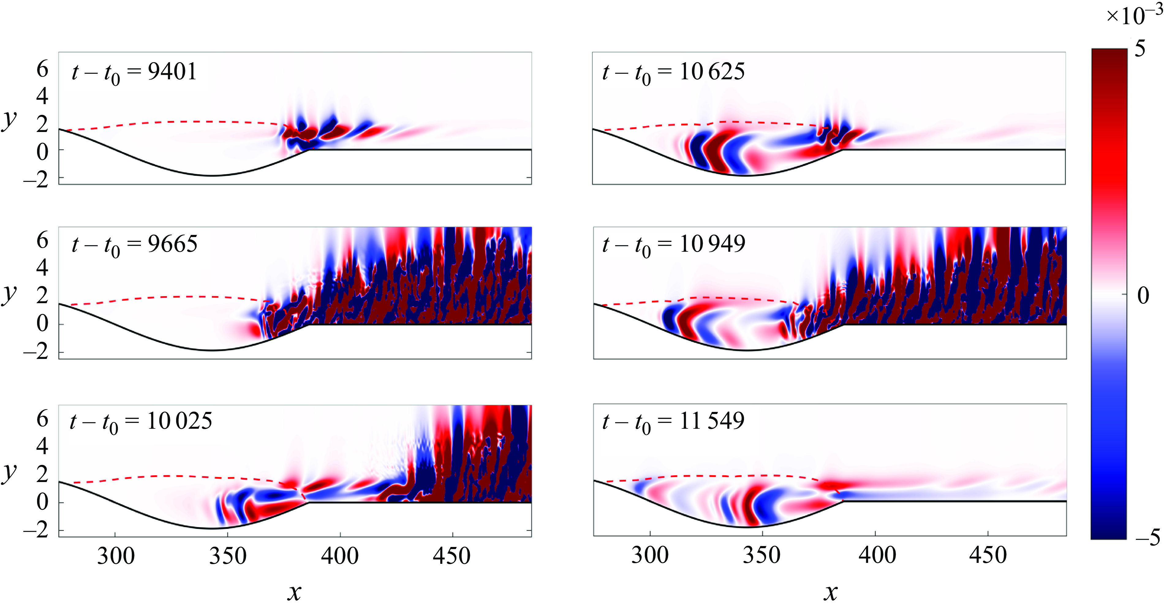
Figure 26. Spanwise perturbation velocity for six different times plotted at the spanwise plane with peak negative base flow distortion. The red dashed line shows the location of instantaneous dividing streamline. The colour bar is saturated to visualise the flow structures. The figure is not drawn to scale.
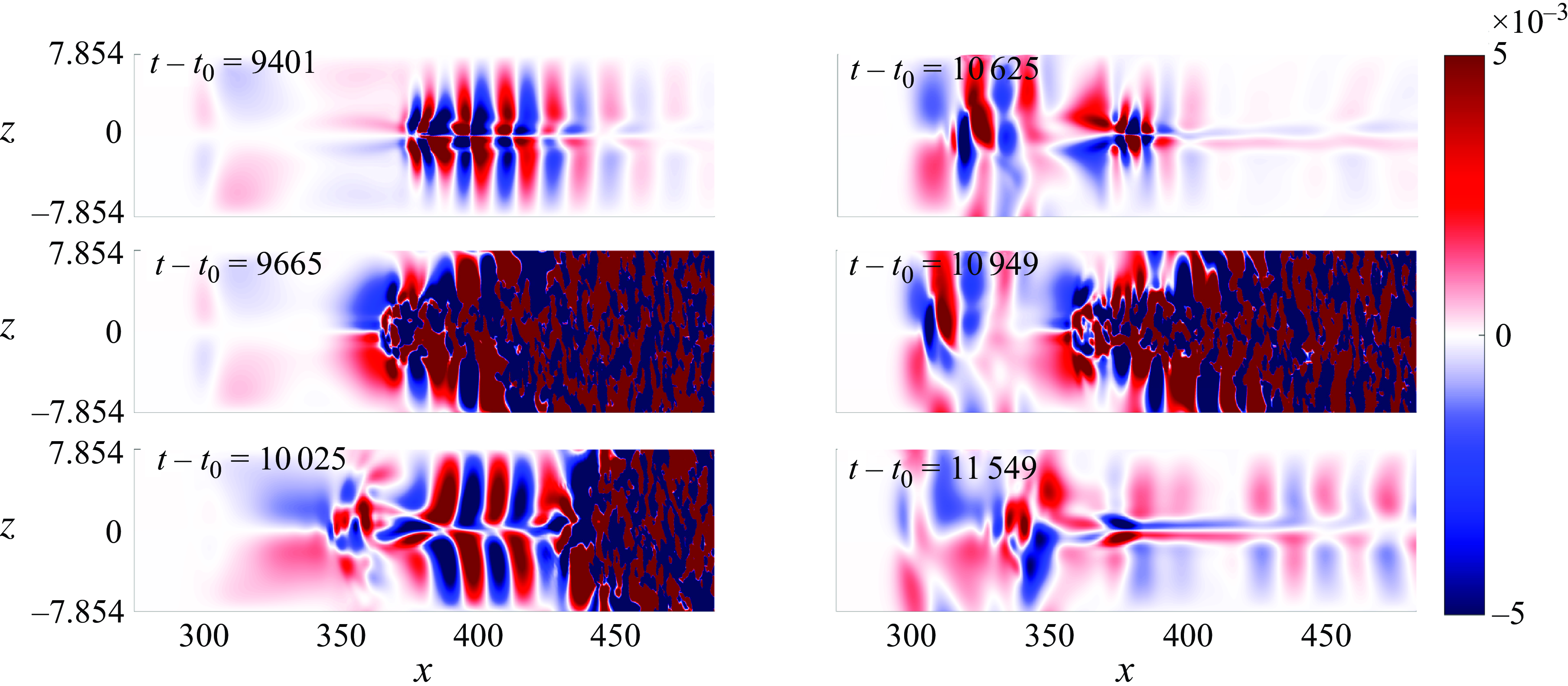
Figure 27. Spanwise perturbation velocity for six different times plotted for a plane parallel to the wall that passes through the peak negative base flow distortion. The colour bar is saturated to visualise the flow structures. The figure is not drawn to scale.
The first panel, at $t'=9401$
, shows the evolution of self-excited secondary instabilities while still they are growing exponentially (figure 24). At this time instance the bubble height is close to its maximum. The shape of the perturbations is the same as the global eigenmode obtained by the secondary instability analysis. Note that since the
$t'=9401$
, shows the evolution of self-excited secondary instabilities while still they are growing exponentially (figure 24). At this time instance the bubble height is close to its maximum. The shape of the perturbations is the same as the global eigenmode obtained by the secondary instability analysis. Note that since the $u$
component is global mode being symmetric (figure 20), the spanwise component must be antisymmetric, which is visible in figure 27 at
$u$
component is global mode being symmetric (figure 20), the spanwise component must be antisymmetric, which is visible in figure 27 at $t'=9401$
. Shortly after the secondary instability saturates and nonlinear interactions become more intense, the disturbance energy reaches a saturated state and a turbulent burst is formed in the aft part of the recirculation bubble, as can be seen in the second panel at
$t'=9401$
. Shortly after the secondary instability saturates and nonlinear interactions become more intense, the disturbance energy reaches a saturated state and a turbulent burst is formed in the aft part of the recirculation bubble, as can be seen in the second panel at $t'=9665$
. Close to the reattachment point (
$t'=9665$
. Close to the reattachment point ( $x\approx 370$
), spanwise perturbations start to create a boomerang-shape structure, which becomes more evident as the leading edge of the perturbation leaves the bubble and the height of the bubble is close to its minimum. The boomerang-like structures then start to propagate upstream within the bubble (third panel at
$x\approx 370$
), spanwise perturbations start to create a boomerang-shape structure, which becomes more evident as the leading edge of the perturbation leaves the bubble and the height of the bubble is close to its minimum. The boomerang-like structures then start to propagate upstream within the bubble (third panel at $t'=10\,025$
). Note that after the boomerang-shape structures are formed in the flow, the symmetry of the flow structure is broken as can be seen in figure 27 at
$t'=10\,025$
). Note that after the boomerang-shape structures are formed in the flow, the symmetry of the flow structure is broken as can be seen in figure 27 at $t'=10\,025$
. Afterwards, the bubble relaminarises and gradually expands in the wall-normal direction (phase P in figure 24), while the spanwise perturbations that emerged from the vicinity of reattachment in the previous turbulent burst keep propagating upstream in the bubble. Eventually, self-excited oscillations reappear as can be seen in the first panel of the right column at
$t'=10\,025$
. Afterwards, the bubble relaminarises and gradually expands in the wall-normal direction (phase P in figure 24), while the spanwise perturbations that emerged from the vicinity of reattachment in the previous turbulent burst keep propagating upstream in the bubble. Eventually, self-excited oscillations reappear as can be seen in the first panel of the right column at $t'=10\,625$
. The formation of the boomerang-like spanwise perturbations is visible from the second panel of the right column at
$t'=10\,625$
. The formation of the boomerang-like spanwise perturbations is visible from the second panel of the right column at $t'=10\,949$
. Since the propagation speed of the perturbations decreases as they get closer to the separation point, the new perturbations originated in the second turbulent burst reach and interact with those from the first burst and create more complex structures, as can be seen from the third panel at
$t'=10\,949$
. Since the propagation speed of the perturbations decreases as they get closer to the separation point, the new perturbations originated in the second turbulent burst reach and interact with those from the first burst and create more complex structures, as can be seen from the third panel at $t'=11\,549$
. The same cycle is repeated for later times as shown by figure 23.
$t'=11\,549$
. The same cycle is repeated for later times as shown by figure 23.
The upstream-propagating boomerang-like structures resemble a family of stable, low-frequency eigenmodes recovered by the global stability analyses. Figure 28( $a$
–
$a$
– $c$
) show the spanwise velocity component of three global eigenmodes of the saturated flow
$c$
) show the spanwise velocity component of three global eigenmodes of the saturated flow $\boldsymbol{u}_{3D}$
, marked by Ms1, Ms2 and Ms3 in the part of the spectrum shown in panel (
$\boldsymbol{u}_{3D}$
, marked by Ms1, Ms2 and Ms3 in the part of the spectrum shown in panel ( $e$
). Panel (
$e$
). Panel ( $d$
) shows the three-dimensional shape of the Ms3 mode. The structures are very similar to the shape of the perturbations shown in figures 26 and 27, although the streamwise wavelength observed in the DNS is not the same as the wavelength of the individual eigenmodes shown in figure 28.
$d$
) shows the three-dimensional shape of the Ms3 mode. The structures are very similar to the shape of the perturbations shown in figures 26 and 27, although the streamwise wavelength observed in the DNS is not the same as the wavelength of the individual eigenmodes shown in figure 28.
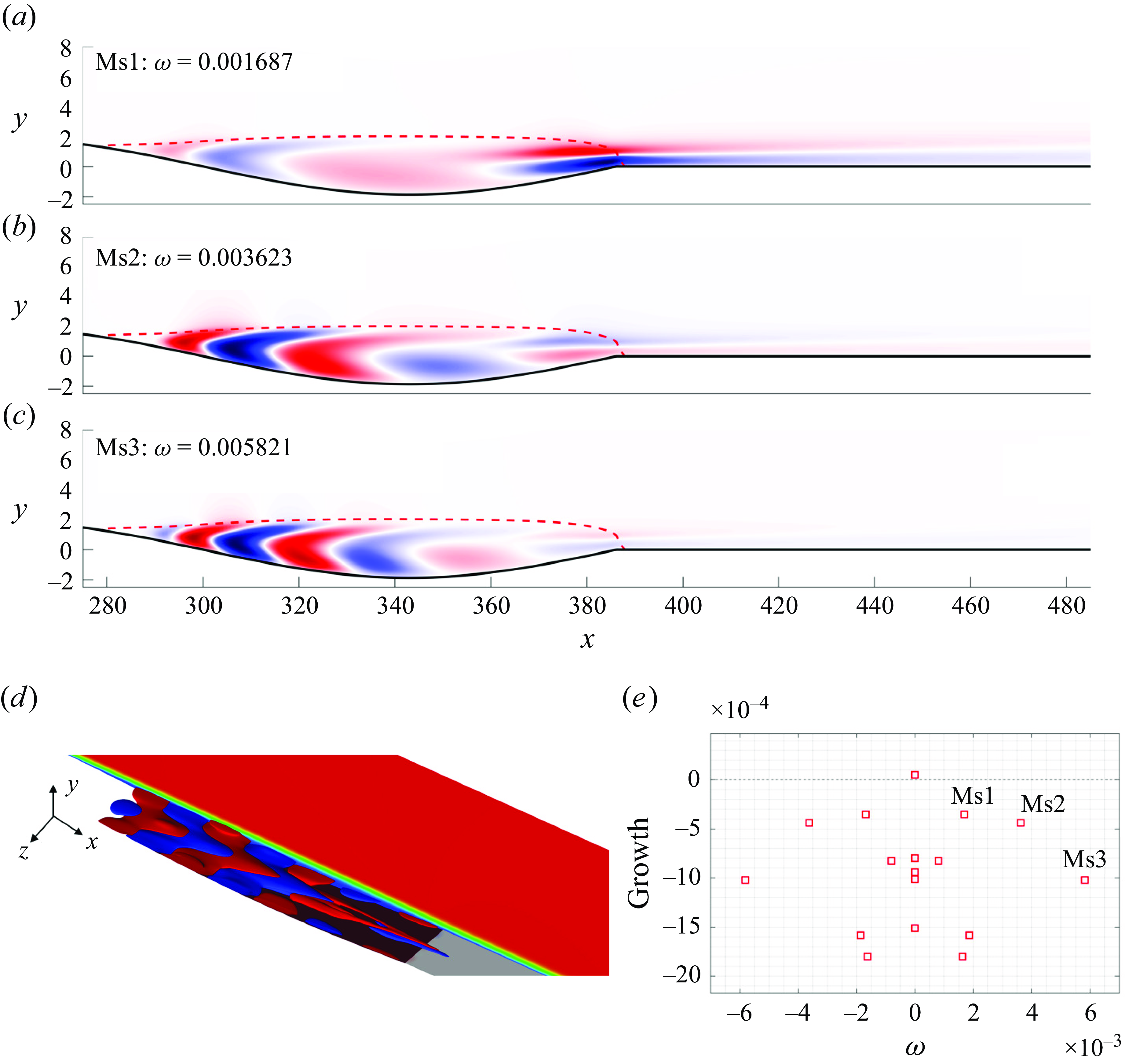
Figure 28. ( $a$
–
$a$
– $c$
) Spanwise velocity component (real part) of global eigenmodes labelled by Ms1, Ms2 and Ms3 in panel (
$c$
) Spanwise velocity component (real part) of global eigenmodes labelled by Ms1, Ms2 and Ms3 in panel ( $e$
), at the spanwise plane with peak negative base flow distortion. (
$e$
), at the spanwise plane with peak negative base flow distortion. ( $d$
) Three-dimensional view of the spanwise velocity field of the Ms3 mode. The red and blue colours show positive and negative values, respectively. (
$d$
) Three-dimensional view of the spanwise velocity field of the Ms3 mode. The red and blue colours show positive and negative values, respectively. ( $e$
) Eigenspectrum corresponding to global stability analysis of the saturated flow
$e$
) Eigenspectrum corresponding to global stability analysis of the saturated flow $\boldsymbol{u}_{3D}$
(same as the inset in figure 19). Panels (
$\boldsymbol{u}_{3D}$
(same as the inset in figure 19). Panels ( $a$
-
$a$
- $c$
) are not drawn to scale.
$c$
) are not drawn to scale.
The same family of eigenmodes is found in the global stability analysis of the two-dimensional base flow $\boldsymbol{u}_0$
(figure 36). However, the shape of the eigenmodes in the spanwise direction is modified on account of the absence of the spanwise distortion that defines the saturated flow. An adjoint sensitivity analysis (analogous to that by Giannetti & Luchini Reference Giannetti and Luchini2007) has been done for the same family of eigenmodes corresponding to the two-dimensional base flow; the region slightly upstream of the reattachment point, located in the vicinity of the peak negative base flow distortion was found to be the most sensitive region. It should be noted that the adjoint sensitivity analysis is not done for the saturated state due to its very high computational cost. However, since the low-frequency eigenmodes for both two-dimensional and saturated flows share many similarities, it is conjectured that the sensitivity characteristics of them are also similar.
$\boldsymbol{u}_0$
(figure 36). However, the shape of the eigenmodes in the spanwise direction is modified on account of the absence of the spanwise distortion that defines the saturated flow. An adjoint sensitivity analysis (analogous to that by Giannetti & Luchini Reference Giannetti and Luchini2007) has been done for the same family of eigenmodes corresponding to the two-dimensional base flow; the region slightly upstream of the reattachment point, located in the vicinity of the peak negative base flow distortion was found to be the most sensitive region. It should be noted that the adjoint sensitivity analysis is not done for the saturated state due to its very high computational cost. However, since the low-frequency eigenmodes for both two-dimensional and saturated flows share many similarities, it is conjectured that the sensitivity characteristics of them are also similar.
These observations suggest that the upstream-propagating spanwise perturbations are associated with the low-frequency stable eigenmodes, which get excited through the interactions with the self-excited secondary instabilities upstream of the reattachment point. For further analysis, a three-dimensional resolvent analysis could be done, but this is out of the scope of the present study. After their nonlinear excitation, these eigenmodes can describe a non-modal behaviour or interact nonlinearly, explaining why the wavelength of the perturbations from DNS is not constant and does not match the individual wavelength of the global stability eigenmodes.
6.2.
Case E,
$\beta =0.6$

The global stability analyses presented in § 4 show that the two-dimensional base flow for case E sustains both two-dimensional oscillatory and three-dimensional steady unstable eigenmodes. Nonlinear DNS simulations with $\beta =0.6$ $(L_z=2\pi /0.6)$
are performed to investigate the interactions between the unstable modes and their subsequent evolution. Details of the DNS domain size and grid are given in Appendix A.3.
$(L_z=2\pi /0.6)$
are performed to investigate the interactions between the unstable modes and their subsequent evolution. Details of the DNS domain size and grid are given in Appendix A.3.
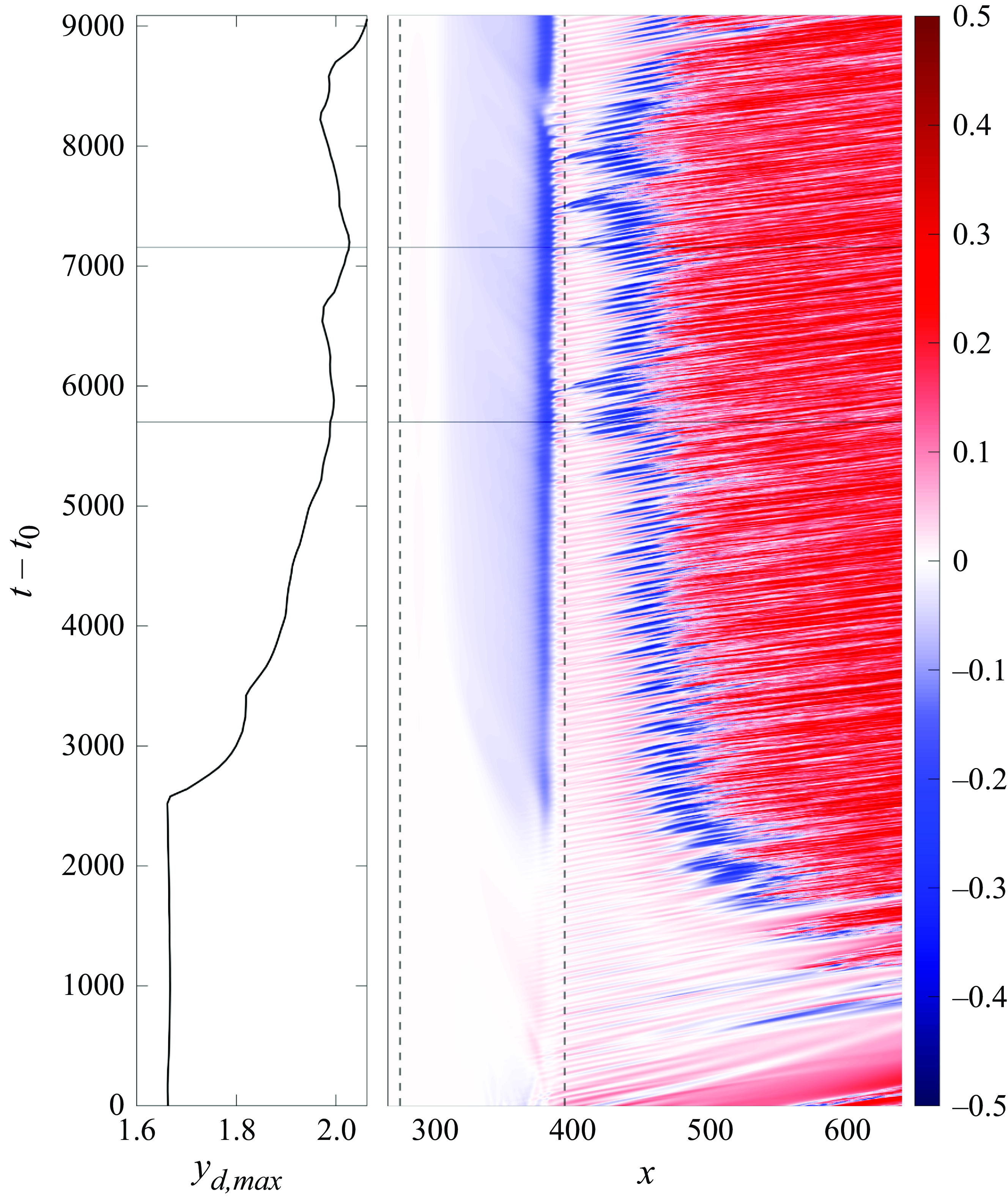
Figure 29. Maximum $y$
coordinate of dividing streamline in the streamwise plane with peak negative base flow distortion (left panel). Spatio-temporal diagram for the
$y$
coordinate of dividing streamline in the streamwise plane with peak negative base flow distortion (left panel). Spatio-temporal diagram for the $u$
component of perturbation velocity for case E,
$u$
component of perturbation velocity for case E, $\beta =0.6$
, for a line parallel to and with distance
$\beta =0.6$
, for a line parallel to and with distance $\Delta y \approx 1.45$
from the wall at the same plane (right panel). Perturbations are calculated based on the two-dimensional base flow.
$\Delta y \approx 1.45$
from the wall at the same plane (right panel). Perturbations are calculated based on the two-dimensional base flow.
Figure 29 shows the $x$
–
$x$
– $t$
diagram for streamwise perturbation velocity (calculated with respect to the initial two-dimensional base flow
$t$
diagram for streamwise perturbation velocity (calculated with respect to the initial two-dimensional base flow $\boldsymbol{u}_0$
) at the spanwise plane with peak negative base flow distortion, for a plane parallel to the wavy wall and separated by a distance
$\boldsymbol{u}_0$
) at the spanwise plane with peak negative base flow distortion, for a plane parallel to the wavy wall and separated by a distance $\Delta y \approx 1.45$
from it. An initial transient has been eliminated from the figure. Self-excited vortex shedding, as predicted by global stability analysis (§ 4), develops spontaneously and is identified by the dark blue spots in the figure.
$\Delta y \approx 1.45$
from it. An initial transient has been eliminated from the figure. Self-excited vortex shedding, as predicted by global stability analysis (§ 4), develops spontaneously and is identified by the dark blue spots in the figure.
The growth of three-dimensional instability can be inferred from $t' \approx 2000$
onwards, when the negative base flow distortion increases upstream of the reattachment point. As shown in § 4.2, nonlinear interactions originated by the growth of the spread mode give rise to a spanwise modulation of the bubble. Thus, the total streamwise velocity decreases in the spanwise locations where the base flow distortion inside the bubble is negative, which simultaneously increases the
$t' \approx 2000$
onwards, when the negative base flow distortion increases upstream of the reattachment point. As shown in § 4.2, nonlinear interactions originated by the growth of the spread mode give rise to a spanwise modulation of the bubble. Thus, the total streamwise velocity decreases in the spanwise locations where the base flow distortion inside the bubble is negative, which simultaneously increases the $y$
coordinate of the dividing streamline of the bubble. As a result of the nonlinear distortion of the underlying base flow, the self-excited oscillations originating from the initially two-dimensional unstable eigenmodes experience a spanwise shear and different advection speeds at different spanwise locations. This leads to the formation of
$y$
coordinate of the dividing streamline of the bubble. As a result of the nonlinear distortion of the underlying base flow, the self-excited oscillations originating from the initially two-dimensional unstable eigenmodes experience a spanwise shear and different advection speeds at different spanwise locations. This leads to the formation of $\Lambda$
vortices with a spanwise wavelength equal to the fundamental spanwise wavelength of the dominant three-dimensional global mode, where the legs of the vortex lie at the spanwise planes with peak negative perturbation inside the bubble. The
$\Lambda$
vortices with a spanwise wavelength equal to the fundamental spanwise wavelength of the dominant three-dimensional global mode, where the legs of the vortex lie at the spanwise planes with peak negative perturbation inside the bubble. The $\Lambda$
vortices turn into hairpin vortices as they travel downstream and their breakdown triggers a rapid transition to turbulence. The formation of these vortices is shown in figure 30.
$\Lambda$
vortices turn into hairpin vortices as they travel downstream and their breakdown triggers a rapid transition to turbulence. The formation of these vortices is shown in figure 30.
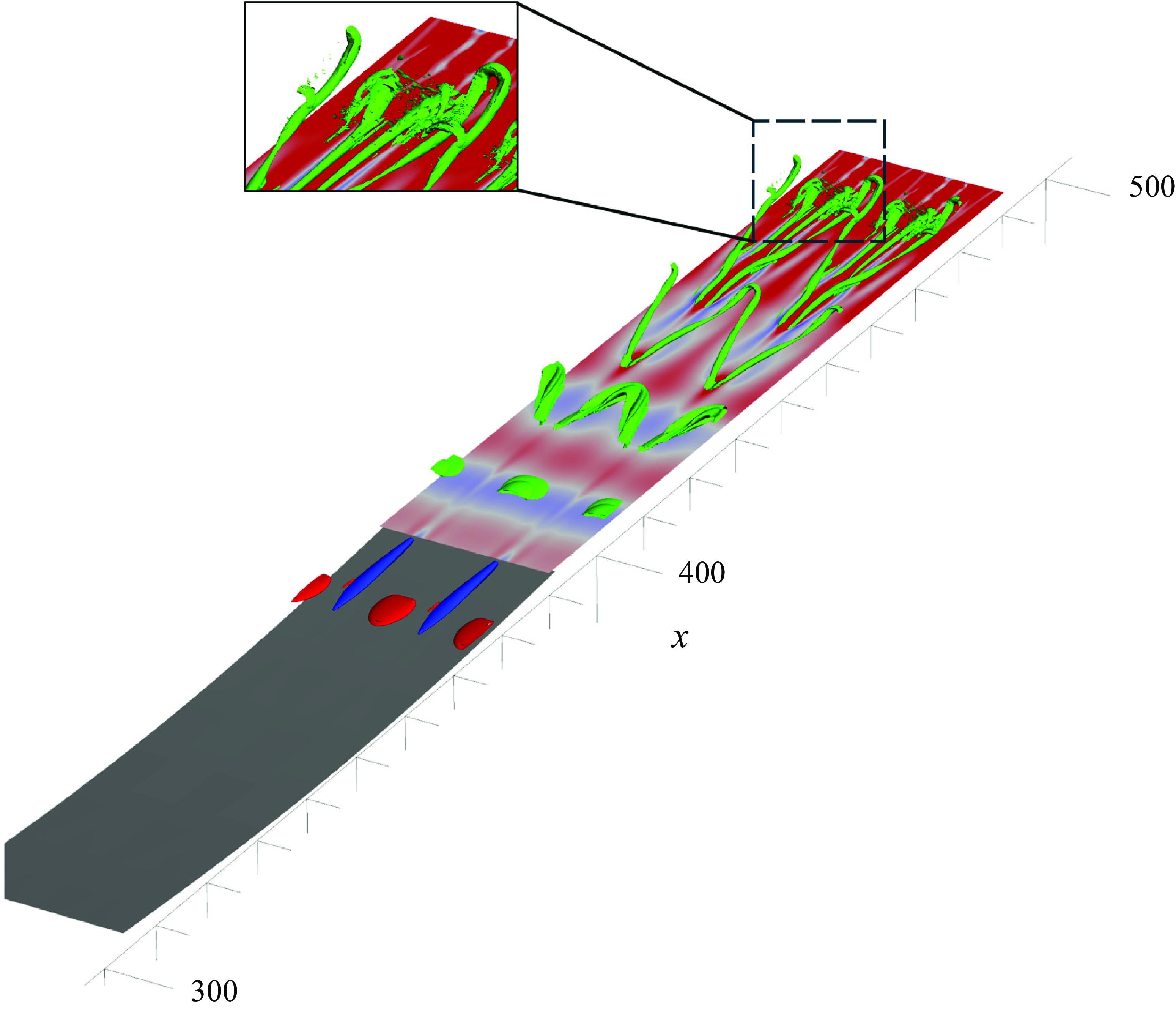
Figure 30. Instantaneous $\lambda _2$
visualizations of the vortical structures in the flow (green isosurfaces) at
$\lambda _2$
visualizations of the vortical structures in the flow (green isosurfaces) at $t'=2570$
. The blue and red colour show the negative (
$t'=2570$
. The blue and red colour show the negative ( $u'=-0.05$
) and positive (
$u'=-0.05$
) and positive ( $u'=0.03$
) isosurfaces of streamwise perturbation velocity inside the bubble. The horizontal plane shows the streamwise perturbation velocity for a plane at
$u'=0.03$
) isosurfaces of streamwise perturbation velocity inside the bubble. The horizontal plane shows the streamwise perturbation velocity for a plane at $y=0.2$
. The figure is shown only for a reduced part of the domain (
$y=0.2$
. The figure is shown only for a reduced part of the domain ( $300\lt x\lt 485$
). For
$300\lt x\lt 485$
). For $\lambda _2$
visualizations, for
$\lambda _2$
visualizations, for $x\lt 435$
, isosurfaces of
$x\lt 435$
, isosurfaces of $\lambda _2=-0.0006$
and for
$\lambda _2=-0.0006$
and for $x\gt 435$
, isosurfaces corresponding to
$x\gt 435$
, isosurfaces corresponding to $\lambda _2=-0.005$
are plotted. Two spanwise periods of the simulation domain are shown.
$\lambda _2=-0.005$
are plotted. Two spanwise periods of the simulation domain are shown.
6.2.1. Unsteady flow characteristics
To analyse the complex three-dimensional vortex shedding and ensuing laminar–turbulent transition, spectral proper orthogonal decomposition (SPOD) is used (Schmidt & Colonius Reference Schmidt and Colonius2020). The cross-spectral density employed is based on the kinetic energy. Here, the data from $t'\approx 2400$
to the end of the simulation (figure 29), which consist of 11 500 three-dimensional snapshots, are divided into blocks of 1150 snapshots with
$t'\approx 2400$
to the end of the simulation (figure 29), which consist of 11 500 three-dimensional snapshots, are divided into blocks of 1150 snapshots with $50 \,\%$
overlap (19 blocks in total). This leads to a frequency-domain discretization with
$50 \,\%$
overlap (19 blocks in total). This leads to a frequency-domain discretization with $\Delta \omega =0.0091$
and Nyquist frequency
$\Delta \omega =0.0091$
and Nyquist frequency $\omega _{max} = 5.23$
. Figure 31 shows the SPOD energy of the leading mode (the black solid line), while the red dashed line in the figure shows the sum of the energy of all SPOD modes for each frequency.
$\omega _{max} = 5.23$
. Figure 31 shows the SPOD energy of the leading mode (the black solid line), while the red dashed line in the figure shows the sum of the energy of all SPOD modes for each frequency.
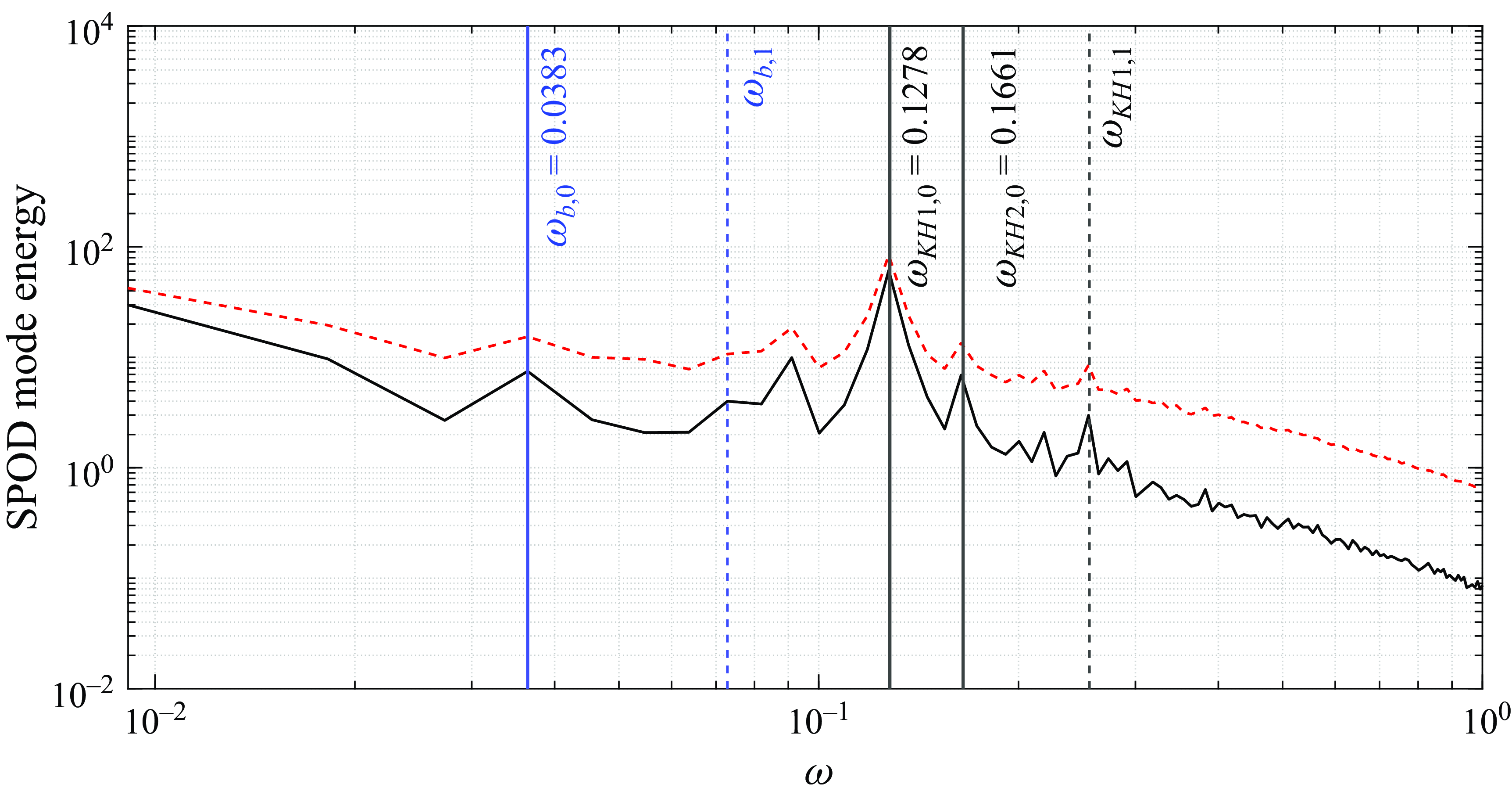
Figure 31. Leading SPOD mode energy in the domain. The red dashed line represents the sum of the energy of all SPOD modes for each frequency.
The SPOD spectrum presents several clear peaks. Vertical solid lines denote specific low and high frequencies, while dashed lines represent higher harmonics of each frequency indicated by the same colour. Starting from high-frequency peaks, the black solid lines specify two frequencies named $\omega _{\textit{KH}1,0}=0.1278$
and
$\omega _{\textit{KH}1,0}=0.1278$
and $\omega _{\textit{KH}2,0}=0.1661$
that are very close to the frequency of two unstable two-dimensional global modes for case E (
$\omega _{\textit{KH}2,0}=0.1661$
that are very close to the frequency of two unstable two-dimensional global modes for case E ( $\omega _{\textit{KH}1,LST}=0.1280$
and
$\omega _{\textit{KH}1,LST}=0.1280$
and $\omega _{\textit{KH}2,LST}=0.1650$
), as shown in figure 8. Note the higher peak for
$\omega _{\textit{KH}2,LST}=0.1650$
), as shown in figure 8. Note the higher peak for $\omega _{\textit{KH}1,0}$
than for
$\omega _{\textit{KH}1,0}$
than for $\omega _{\textit{KH}2,0}$
that is in agreement with the higher growth rate of
$\omega _{\textit{KH}2,0}$
that is in agreement with the higher growth rate of $\omega _{\textit{KH}1,LST}$
compared with
$\omega _{\textit{KH}1,LST}$
compared with $\omega _{\textit{KH}2,LST}$
, as figure 8 shows. The black dashed line specifies the first harmonic
$\omega _{\textit{KH}2,LST}$
, as figure 8 shows. The black dashed line specifies the first harmonic $(\omega _{\textit{KH}1,1})$
of
$(\omega _{\textit{KH}1,1})$
of $\omega _{\textit{KH}1,0}$
. The frequency peak at
$\omega _{\textit{KH}1,0}$
. The frequency peak at $\omega =0.0894$
is also very close to the frequency of a globally stable mode with
$\omega =0.0894$
is also very close to the frequency of a globally stable mode with $\omega =0.0882$
in the eigenmode spectrum shown in figure 8. Figure 32 shows the real part of the leading SPOD mode at
$\omega =0.0882$
in the eigenmode spectrum shown in figure 8. Figure 32 shows the real part of the leading SPOD mode at $\omega =0.1278$
for two spanwise periods and for
$\omega =0.1278$
for two spanwise periods and for $x\lt 485$
. This mode consists of spanwise-modulated rollers appearing just downstream of the reattachment point and extending further downstream. Its spatial shape resembles the hairpin vortices from figure 30, where the heads of the hairpin vortices are again visible at
$x\lt 485$
. This mode consists of spanwise-modulated rollers appearing just downstream of the reattachment point and extending further downstream. Its spatial shape resembles the hairpin vortices from figure 30, where the heads of the hairpin vortices are again visible at $z\approx \pm 5$
and
$z\approx \pm 5$
and $z\approx 15$
. Moreover, the SPOD mode exhibits other sets of hairpin-like structures that appear farther downstream (from
$z\approx 15$
. Moreover, the SPOD mode exhibits other sets of hairpin-like structures that appear farther downstream (from $x\approx 470$
) and present a different spanwise phase compared with the fundamental vortices: i.e. their heads are in the spanwise plane with peak negative base flow distortion inside the bubble (
$x\approx 470$
) and present a different spanwise phase compared with the fundamental vortices: i.e. their heads are in the spanwise plane with peak negative base flow distortion inside the bubble ( $z\approx 0$
). These secondary hairpin vortices are also observed in DNS and can be seen in the magnified view shown in figure 30. Note that the SPOD mode corresponds to
$z\approx 0$
). These secondary hairpin vortices are also observed in DNS and can be seen in the magnified view shown in figure 30. Note that the SPOD mode corresponds to $\omega _{\textit{KH}2,0}=0.1661$
(not shown here) is very similar to the one for
$\omega _{\textit{KH}2,0}=0.1661$
(not shown here) is very similar to the one for $\omega _{\textit{KH}1,0}=0.1278$
.
$\omega _{\textit{KH}1,0}=0.1278$
.
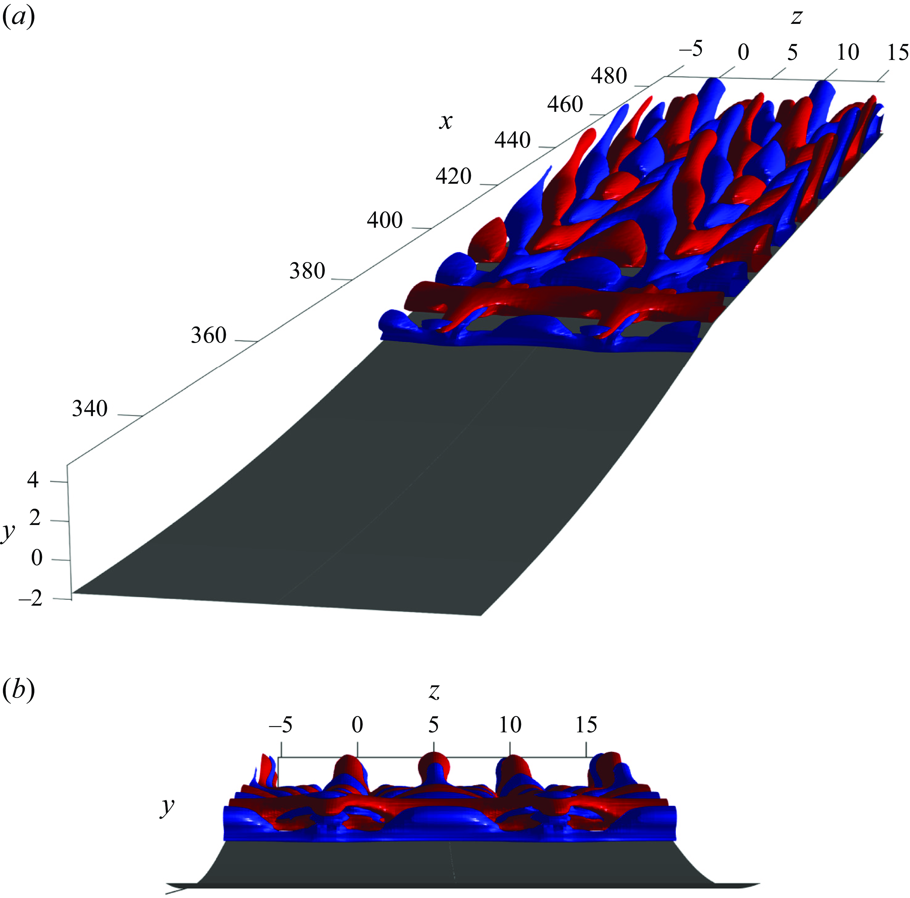
Figure 32. Real part of the $u$
component of the leading SPOD mode for
$u$
component of the leading SPOD mode for $\omega =0.1278$
. Red and blue colours correspond to
$\omega =0.1278$
. Red and blue colours correspond to ${u}'=\pm 0.0015$
and
${u}'=\pm 0.0015$
and $u'=-0.0015$
, respectively. Two spanwise periods of the simulation are shown for visualization.
$u'=-0.0015$
, respectively. Two spanwise periods of the simulation are shown for visualization.
The low-frequency oscillations, on the other hand, cannot be directly related to two-dimensional self-excited mechanisms as there is no low-frequency unstable mode in the global spectrum for this case. In the absence of external forcing, as is the case here, they must be due either to interactions between high-frequency oscillations or to the nonlinearities resulting from the growth of three-dimensional instabilities and base flow distortion. The blue solid line specifies a low-frequency peak with $\omega =0.0383$
. Interestingly, this frequency is equal to the difference between the frequency of
$\omega =0.0383$
. Interestingly, this frequency is equal to the difference between the frequency of $\omega _{\textit{KH}1,0}$
and
$\omega _{\textit{KH}1,0}$
and $\omega _{\textit{KH}2,0}$
, i.e. the beating frequency due to the interaction of
$\omega _{\textit{KH}2,0}$
, i.e. the beating frequency due to the interaction of $\omega _{\textit{KH}1,0}$
and
$\omega _{\textit{KH}1,0}$
and $\omega _{\textit{KH}2,0}$
. The first harmonic of this frequency is also specified by the blue dashed line in the figure. The high energy content in the very low-frequency range (
$\omega _{\textit{KH}2,0}$
. The first harmonic of this frequency is also specified by the blue dashed line in the figure. The high energy content in the very low-frequency range ( $\omega \lt 0.03$
) suggests that there might still be low-frequency dynamics in the SPOD spectrum that requires much longer time series to be resolved. The low-frequency, high energy content in the separation bubbles is attributed to the so-called breathing or flapping of the bubble (Zaman et al. Reference Zaman, Mckinzie and Rumsey1989; Sigurdson Reference Sigurdson1995), i.e. a quasi-periodic vertical movement of the separated shear layer from the wall. This very low-frequency vertical movement of the bubble is shown in the left panel of figure 29. Furthermore, when the height of the bubble increases, a strong vortex is shed from the bubble that results in the formation of a
$\omega \lt 0.03$
) suggests that there might still be low-frequency dynamics in the SPOD spectrum that requires much longer time series to be resolved. The low-frequency, high energy content in the separation bubbles is attributed to the so-called breathing or flapping of the bubble (Zaman et al. Reference Zaman, Mckinzie and Rumsey1989; Sigurdson Reference Sigurdson1995), i.e. a quasi-periodic vertical movement of the separated shear layer from the wall. This very low-frequency vertical movement of the bubble is shown in the left panel of figure 29. Furthermore, when the height of the bubble increases, a strong vortex is shed from the bubble that results in the formation of a $\Lambda$
vortex (with head located at
$\Lambda$
vortex (with head located at $z\approx 0$
) just downstream of the reattachment point. This corresponds to the dark blue spots downstream of the reattachment point coincident with the increase of the bubble height (marked by horizontal solid lines in figure 29). Figure 33 shows
$z\approx 0$
) just downstream of the reattachment point. This corresponds to the dark blue spots downstream of the reattachment point coincident with the increase of the bubble height (marked by horizontal solid lines in figure 29). Figure 33 shows $\lambda _2$
visualization of the vortical structures at
$\lambda _2$
visualization of the vortical structures at $t'=6000$
. The hairpin vortices downstream of the reattachment point are highlighted in the magnified view of the figure.
$t'=6000$
. The hairpin vortices downstream of the reattachment point are highlighted in the magnified view of the figure.
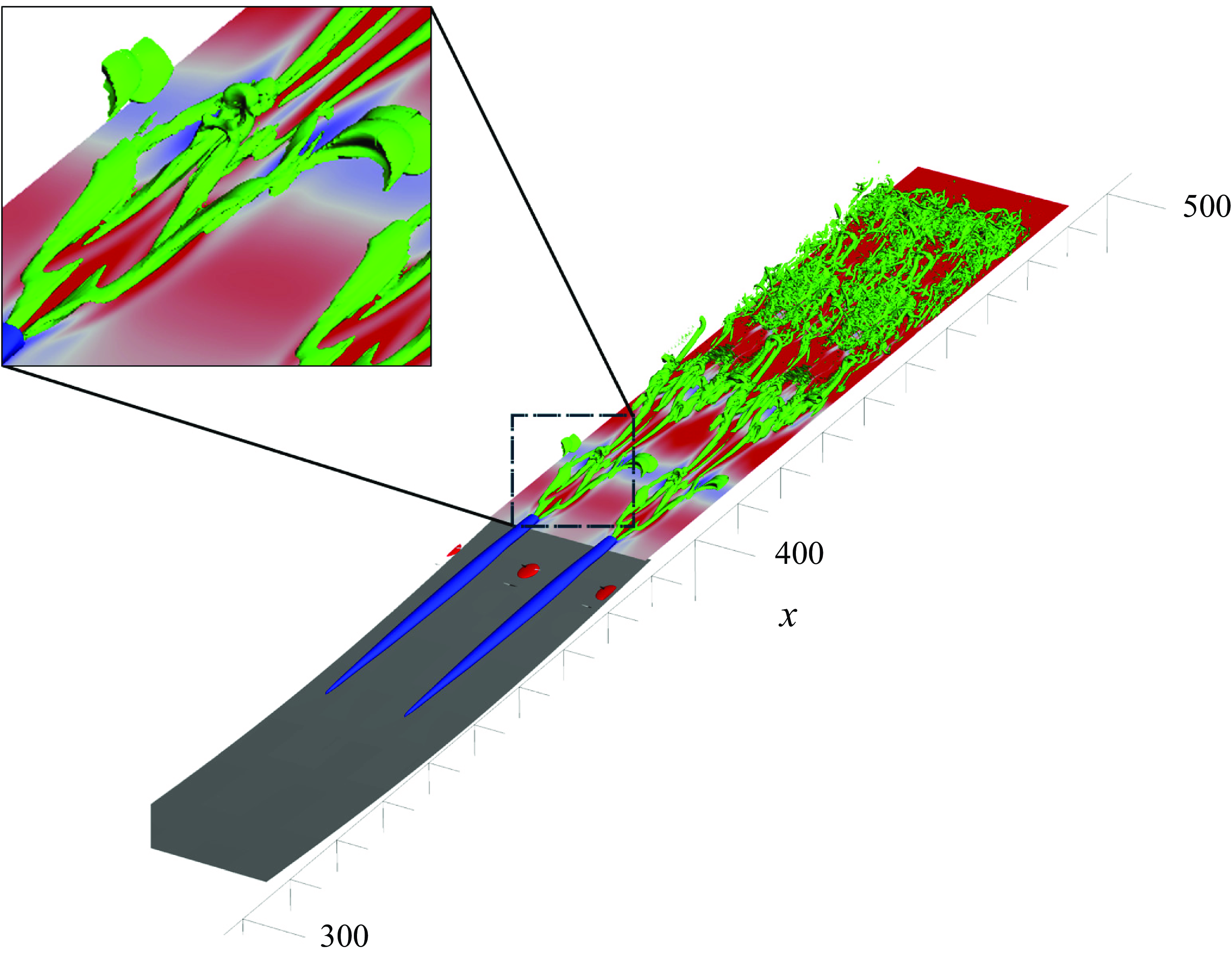
Figure 33. Instantaneous $\lambda _2$
visualizations of the vortical structures in the flow (green isosurfaces) at
$\lambda _2$
visualizations of the vortical structures in the flow (green isosurfaces) at $t'=6000$
. The blue and red colours show the negative (
$t'=6000$
. The blue and red colours show the negative ( $u'=-0.05$
) and positive (
$u'=-0.05$
) and positive ( $u'=0.055$
) isosurfaces of streamwise perturbation velocity inside the bubble. The horizontal plane shows the streamwise perturbation velocity for a plane at
$u'=0.055$
) isosurfaces of streamwise perturbation velocity inside the bubble. The horizontal plane shows the streamwise perturbation velocity for a plane at $y=0.2$
. The figure is shown only for a part of the domain (
$y=0.2$
. The figure is shown only for a part of the domain ( $300\lt x\lt 485$
). For
$300\lt x\lt 485$
). For $\lambda _2$
visualizations, for
$\lambda _2$
visualizations, for $x\lt 435$
, isosurfaces corresponding to
$x\lt 435$
, isosurfaces corresponding to $\lambda _2=-0.002$
are plotted and, for
$\lambda _2=-0.002$
are plotted and, for $x\gt 435$
, isosurfaces corresponding to
$x\gt 435$
, isosurfaces corresponding to $\lambda _2=-0.08$
are plotted. Note that two spanwise periods of the simulation are shown for visualization.
$\lambda _2=-0.08$
are plotted. Note that two spanwise periods of the simulation are shown for visualization.
7. Conclusions
This study investigates the stability characteristics and transition to turbulence of a series of wall-waviness-induced LSBs in the absence of incoming disturbances or external forcing. Considering steady spanwise-homogeneous (two-dimensional) solutions of the governing equations, an empirical relation is determined between the waviness height and wavelength and the Reynolds number based on the local thickness of the boundary layer that delimits the occurrence of flow separation. Using this relation, a set of base LSBs with different lengths and reverse flow intensities are constructed. Their two- and three-dimensional instability characteristics and subsequent self-excited transition scenarios are investigated in detail using linear stability theory and DNS.
A global eigenmode analysis shows that bubbles with a peak reversed flow of approximately $10\,\%-12\,\%$
of the free-stream velocity can become globally unstable with respect to two-dimensional instabilities. This value is lower than the threshold of
$10\,\%-12\,\%$
of the free-stream velocity can become globally unstable with respect to two-dimensional instabilities. This value is lower than the threshold of $16\,\%-25\,\%$
proposed by some researchers for the onset of the absolute Kelvin–Helmholtz instability (Hammond & Redekopp Reference Hammond and Redekopp1998; Alam & Sandham Reference Alam and Sandham2000; Rist & Maucher Reference Rist and Maucher2002; Diwan Reference Diwan2009). Incidentally, these bubbles also do not satisfy the geometrical criterion proposed by Avanci et al. (Reference Avanci, Rodríguez and Alves2019), as their local inflection point is always located above the dividing streamline. These observations suggest that they are rather originated by non-parallel or elliptic effects, even if their spatial structure contains Kelvin–Helmholtz disturbances.
$16\,\%-25\,\%$
proposed by some researchers for the onset of the absolute Kelvin–Helmholtz instability (Hammond & Redekopp Reference Hammond and Redekopp1998; Alam & Sandham Reference Alam and Sandham2000; Rist & Maucher Reference Rist and Maucher2002; Diwan Reference Diwan2009). Incidentally, these bubbles also do not satisfy the geometrical criterion proposed by Avanci et al. (Reference Avanci, Rodríguez and Alves2019), as their local inflection point is always located above the dividing streamline. These observations suggest that they are rather originated by non-parallel or elliptic effects, even if their spatial structure contains Kelvin–Helmholtz disturbances.
The three-dimensional instability analysis of the spanwise-homogeneous base flows recovers, for all cases analysed, the self-excited three-dimensional eigenmode typically found in pressure-induced flat-plate LSBs (Theofilis et al. Reference Theofilis, Hein and Dallmann2000; Cherubini et al. Reference Cherubini, Robinet, De Palma and Alizard2010; Rodríguez & Theofilis Reference Rodríguez and Theofilis2010; Rodríguez et al. Reference Rodríguez, Gennaro and Juniper2013). This eigenmode is active almost in the whole bubble and is thus referred to as the ‘spread mode’ here. This mode corresponds to a centrifugal instability and is caused by changes in the curvature of the recirculating streamlines (Bayly Reference Bayly1988; Gallaire et al. Reference Gallaire, Marquillie and Ehrenstein2007). By analysing the recirculating streamlines for the different base flows in this work, additional changes in the streamline curvature are found for some wall-waviness geometries. For these base flows, an additional three-dimensional, zero-frequency eigenmode is consistently found, coexisting with the ‘spread’ mode and with higher growth rates. This mode is localised in the vicinity of the region where the streamlines attain their peak curvature, and vanishes along the separated shear layer. The spatial structure of this ‘localised mode’ also relates it to centrifugal instability.
Analysing the spatial structures of these eigenmodes illustrates more fundamental differences. At a streamwise plane, the real part of the $u$
-velocity component corresponding to the localised mode changes sign inside the recirculation bubble. The effect of this on the nonlinear saturation of the instability is investigated using DNS. It is shown that this property stabilises the structural shape of the bubble near the reattachment point by prohibiting reverse flow to get intensified in that region. In the case of coexistence of the localised and spread modes (case A,
$u$
-velocity component corresponding to the localised mode changes sign inside the recirculation bubble. The effect of this on the nonlinear saturation of the instability is investigated using DNS. It is shown that this property stabilises the structural shape of the bubble near the reattachment point by prohibiting reverse flow to get intensified in that region. In the case of coexistence of the localised and spread modes (case A, $\beta =0.7$
), although the initially spanwise-homogeneous bubble gets strongly modulated and becomes fully three dimensional, no sign of self-excited secondary instability was observed. On the other hand, in the case of the presence of the spread mode alone (case G,
$\beta =0.7$
), although the initially spanwise-homogeneous bubble gets strongly modulated and becomes fully three dimensional, no sign of self-excited secondary instability was observed. On the other hand, in the case of the presence of the spread mode alone (case G, $\beta =0.4$
), the rear part of the bubble expands. As a result, the inflection point present in the separated shear layer crosses the dividing streamline of the bubble (i.e. enters inside the recirculation region) that triggers self-excited secondary instabilities and transition, in agreement with Rodríguez et al. (Reference Rodríguez, Gennaro and Souza2021a
).
$\beta =0.4$
), the rear part of the bubble expands. As a result, the inflection point present in the separated shear layer crosses the dividing streamline of the bubble (i.e. enters inside the recirculation region) that triggers self-excited secondary instabilities and transition, in agreement with Rodríguez et al. (Reference Rodríguez, Gennaro and Souza2021a
).
For the latter case (case G, $\beta =0.4$
), the saturated base flow is obtained using SFD and a three-dimensional stability analysis on the saturated base flow, i.e. a secondary global stability analysis, is performed. The results show two unstable modes with close frequencies and very high growth rates, and a family of low-frequency stable modes. The structure of the unstable modes resembles finite-span (symmetric) Kelvin–Helmholtz instabilities, which are rooted from the region with peak negative base flow distortion inside the bubble. A linear impulse response analysis consistent with the secondary stability analysis is performed, showing a continuous shedding from the rear part of the bubble with structures similar to the global modes.
$\beta =0.4$
), the saturated base flow is obtained using SFD and a three-dimensional stability analysis on the saturated base flow, i.e. a secondary global stability analysis, is performed. The results show two unstable modes with close frequencies and very high growth rates, and a family of low-frequency stable modes. The structure of the unstable modes resembles finite-span (symmetric) Kelvin–Helmholtz instabilities, which are rooted from the region with peak negative base flow distortion inside the bubble. A linear impulse response analysis consistent with the secondary stability analysis is performed, showing a continuous shedding from the rear part of the bubble with structures similar to the global modes.
Nonlinear simulations are then performed to study the ensuing transition scenarios for two selected cases. In the first case (case G, $\beta =0.4$
), the two-dimensional base bubble is unstable with respect to one (spread) three-dimensional global mode. After the initial transient, a quasi-periodic turbulent burst cycle is identified. Analysing the temporal evolution of the kinetic energy of perturbations in the domain reveals that this quasi-periodic burst cycles consists of three mechanisms corresponding to (i) spanwise distortion (three-dimensionalisation) of the bubble due to primary instability, (ii) a sudden increase in energy of the domain due to explosive growth of secondary instabilities, and (iii) formation of a turbulent burst that pulls recirculating fluid downstream, transiently reducing the size of the separation bubble. After the occurrence of each turbulent burst, upstream-propagating disturbances inside the bubble are identified. It is conjectured that these perturbations are associated with the low-frequency stable eigenmodes (found in the spectrum of the system obtained by secondary stability analysis) that get excited through the interactions of self-excited secondary instabilities. In the second case (case E,
$\beta =0.4$
), the two-dimensional base bubble is unstable with respect to one (spread) three-dimensional global mode. After the initial transient, a quasi-periodic turbulent burst cycle is identified. Analysing the temporal evolution of the kinetic energy of perturbations in the domain reveals that this quasi-periodic burst cycles consists of three mechanisms corresponding to (i) spanwise distortion (three-dimensionalisation) of the bubble due to primary instability, (ii) a sudden increase in energy of the domain due to explosive growth of secondary instabilities, and (iii) formation of a turbulent burst that pulls recirculating fluid downstream, transiently reducing the size of the separation bubble. After the occurrence of each turbulent burst, upstream-propagating disturbances inside the bubble are identified. It is conjectured that these perturbations are associated with the low-frequency stable eigenmodes (found in the spectrum of the system obtained by secondary stability analysis) that get excited through the interactions of self-excited secondary instabilities. In the second case (case E, $\beta =0.7$
), the two-dimensional bubble is unstable with respect to both localised and spread three-dimensional modes and also two-dimensional modes representing self-sustained Kelvin-Helmholtz waves. The nonlinear interaction of two-dimensional waves and steady three-dimensional instability results in the formation of
$\beta =0.7$
), the two-dimensional bubble is unstable with respect to both localised and spread three-dimensional modes and also two-dimensional modes representing self-sustained Kelvin-Helmholtz waves. The nonlinear interaction of two-dimensional waves and steady three-dimensional instability results in the formation of $\Lambda$
vortices with a spanwise wavelength equal to the fundamental spanwise wavelength of the dominant three-dimensional global mode. The
$\Lambda$
vortices with a spanwise wavelength equal to the fundamental spanwise wavelength of the dominant three-dimensional global mode. The $\Lambda$
vortices evolve into hairpin vortices as they travel downstream and their breakdown leads to a rapid transition to turbulence.
$\Lambda$
vortices evolve into hairpin vortices as they travel downstream and their breakdown leads to a rapid transition to turbulence.
This work shows that relatively mild surface waviness suffices to induce flow separation and the formation of recirculation bubbles, and that such recirculation bubbles are inherently unstable to self-excited three-dimensional instabilities of a centrifugal nature. The spanwise deformation of the recirculation induced by the instability favours self-excited secondary instabilities in the form of short-span Kelvin-Helmholtz waves. This sequence of instabilities triggers laminar–turbulent transition in the absence of external disturbances. Two different fully nonlinear transition scenarios are described here; other scenarios may also appear owing to minute differences in the nonlinear interactions. Transition scenarios originating from a self-excited instability are usually robust and can prevail even if external disturbances are present. However, the possible interactions between the instabilities discussed herein and external disturbances, like Tollmien–Schlichting waves or streaks arising from the receptivity to FST, should be addressed in future works. Depending on the FST intensity and boundary layer receptivity mechanisms associated with the plate leading edge or surface roughness, the amplitude and characteristics of incoming disturbances can widely vary, altering the scenarios discussed here. The possibilities span from constructive interactions with the self-excited instabilities (Rodríguez & Gennaro Reference Rodríguez and Gennaro2019; Rodríguez et al. Reference Rodríguez, Martini, Cavalieri and Jordan2021b ), to the formation of strongly coherent two-dimensional vortex rolls (Embacher & Fasel Reference Embacher and Fasel2014), to highly complex scenarios in which distinguishing between self-excited and convective instabilities becomes difficult (Hosseinverdi & Fasel Reference Hosseinverdi and Fasel2019), and even to the suppression of laminar separation (Xu & Wu Reference Xu and Wu2021).
Acknowledgements.
The computer resources provided by The National Academic Infrastructure for Supercomputing in Sweden (NAISS) at the Centre for High Performance Computing (PDC) at the Royal Institute of Technology (Stockholm) and National Supercomputer Center (NSC) at Linköping university (Linköping) are gratefully acknowledged.
Funding.
This project has received funding from the European Union’s Horizon 2020 research and innovation programme under the Marie Skłodowska-Curie grant agreement No 955923. D.R. acknowledges funding from the Spanish Ministry of Science, Innovation and Universities and European Union’s FEDER (PID2021–125812OB-C22), and from the Government of the Community of Madrid within the Program of Excellence in Faculty (V-PRICIT line 3).
Declaration of interests.
The authors report no conflict of interest.
Appendix A. Technical details of numerical simulations and grid convergence
In this appendix, technical aspects of numerical simulations, such as the effect of grid and domain size on the solutions of eigenvalue problems and DNS presented through the paper will be discussed.
A.1 Two-dimensional eigenvalue problem: planar (
$\beta =0$
) two-dimensional instabilities

To obtain the results presented in § 4 (figure 8), different Krylov subspace sizes are used for different cases, but typically a subspace of size 250–350 is chosen and the first 50–80 eigenvalues for each subspace size are considered converged, respectively. The results presented in § 4 correspond to a domain size with height and length equal to 700 and 1400, respectively. The convergence with spatial discretisation is also checked by increasing the polynomial order from 7 to 9, which recovers no significant changes in the growth rates or frequency of the unstable modes. The two-dimensional modes being planar are very sensitive to the size of the domain (both length and height) and outlet boundary condition treatment. In the following, the effects these factors on the obtained eigenvalues are investigated.
A.1.1 Effect of height and length of the domain
Figure 34 shows the effect of height and length of the domain on the frequency and growth rate of the two-dimensional global modes for case E. Panel $(a)$
corresponds to a domain with length
$(a)$
corresponds to a domain with length $L=1400$
and different heights, while panel
$L=1400$
and different heights, while panel $(b)$
corresponds to a domain of height
$(b)$
corresponds to a domain of height $H=700$
and different domain lengths. The figure shows that the height of the domain affects the growth rate of both low- and high-frequency modes; choosing the small height for the domain (
$H=700$
and different domain lengths. The figure shows that the height of the domain affects the growth rate of both low- and high-frequency modes; choosing the small height for the domain ( $H=60$
, panel
$H=60$
, panel $(a)$
) results in under-predicting the growth of high-frequency modes. By increasing the height from 400 to 700, no significant changes in the growth of the modes are observed. The length of the domain, on the other hand, mostly affects the growth of low-frequency modes.
$(a)$
) results in under-predicting the growth of high-frequency modes. By increasing the height from 400 to 700, no significant changes in the growth of the modes are observed. The length of the domain, on the other hand, mostly affects the growth of low-frequency modes.
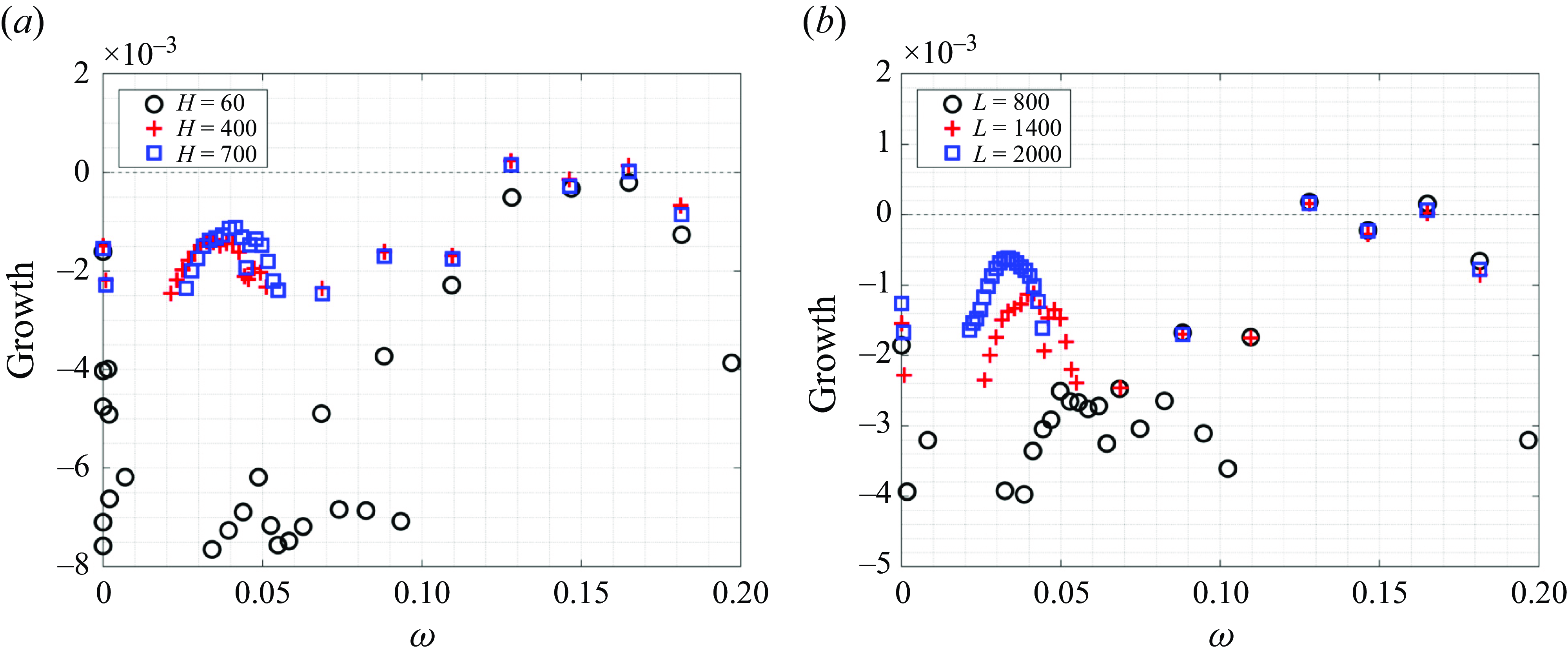
Figure 34. Eigenvalue spectrum for case E. Effect of the height of the domain on the growth of planar global modes for a domain with length $L=1400$ $(a)$
, and the effect of the length of the domain on the growth of modes for a domain with height
$(a)$
, and the effect of the length of the domain on the growth of modes for a domain with height $H=700$ $(b)$
.
$(b)$
.
A.1.2 Effect of fringe layer at outlet on growth rate of two-dimensional low-frequency modes
Figure 35 shows the effect of using a fringe region at the outlet on the growth rates of the global modes. The fringe region acts as a forcing in momentum equations to smoothly force the perturbations to vanish. The strength of the forcing starts to increase smoothly from the last 30 units upstream of the outlet and has full strength for the last 15 units. Other widths for the fringe with different maximum strengths have also been tested, leading to the same results. The fringe region affects the low-frequency region significantly. This may be because the low-frequency modes, as shown in figure 9, extend until the end of the computational domain. If no fringe is used in linear simulations to damp these disturbances at the outlet, the upstream contamination from the outlet makes them artificially unstable. The high-frequency modes, on the other hand, have a localised nature and decay before reaching the outlet of the simulation. Thus, they remain unaffected by the fringe region.
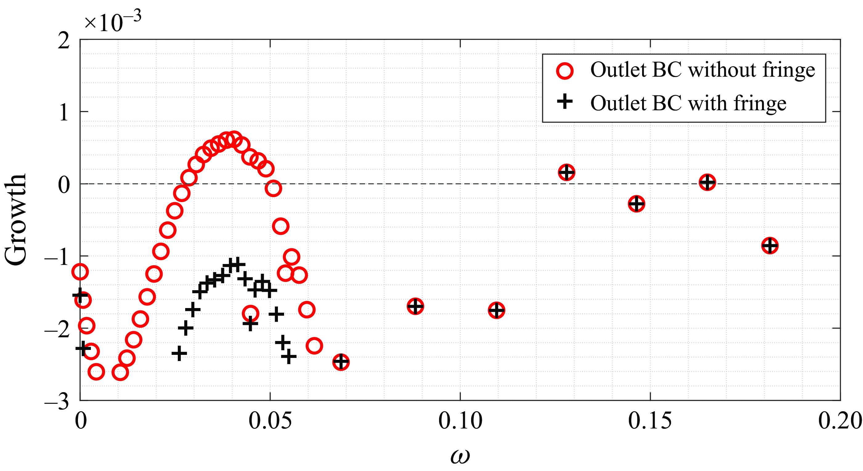
Figure 35. Eigenvalue spectrum for case E with and without using fringe at the outlet boundary condition. A domain with a height of 700 and a length of 1400 is used.
A.2 Two-dimensional eigenvalue problem: three-dimensional (
$\beta \neq 0$
) instabilities

To validate the mapping and the accuracy of the method introduced in § 2.3, the unstable region of the spectrum for case E ( $\beta = 0.6$
) is cross-validated through a time-stepping approach using Nek5000. The differences between the growth of the unstable eigenvalues obtained with these two different methods is found to be negligible (figure 36). The second most unstable mode obtained with Nek5000, which is absent in the solution of the two-dimensional eigenvalue problem, corresponds to the first harmonic (
$\beta = 0.6$
) is cross-validated through a time-stepping approach using Nek5000. The differences between the growth of the unstable eigenvalues obtained with these two different methods is found to be negligible (figure 36). The second most unstable mode obtained with Nek5000, which is absent in the solution of the two-dimensional eigenvalue problem, corresponds to the first harmonic ( $\beta =1.2$
) of the fundamental spanwise wavenumber. The same growth rate as the growth rate calculated with Nek5000 is obtained in the solution of the two-dimensional eigenvalue problem for
$\beta =1.2$
) of the fundamental spanwise wavenumber. The same growth rate as the growth rate calculated with Nek5000 is obtained in the solution of the two-dimensional eigenvalue problem for $\beta =1.2$
.
$\beta =1.2$
.
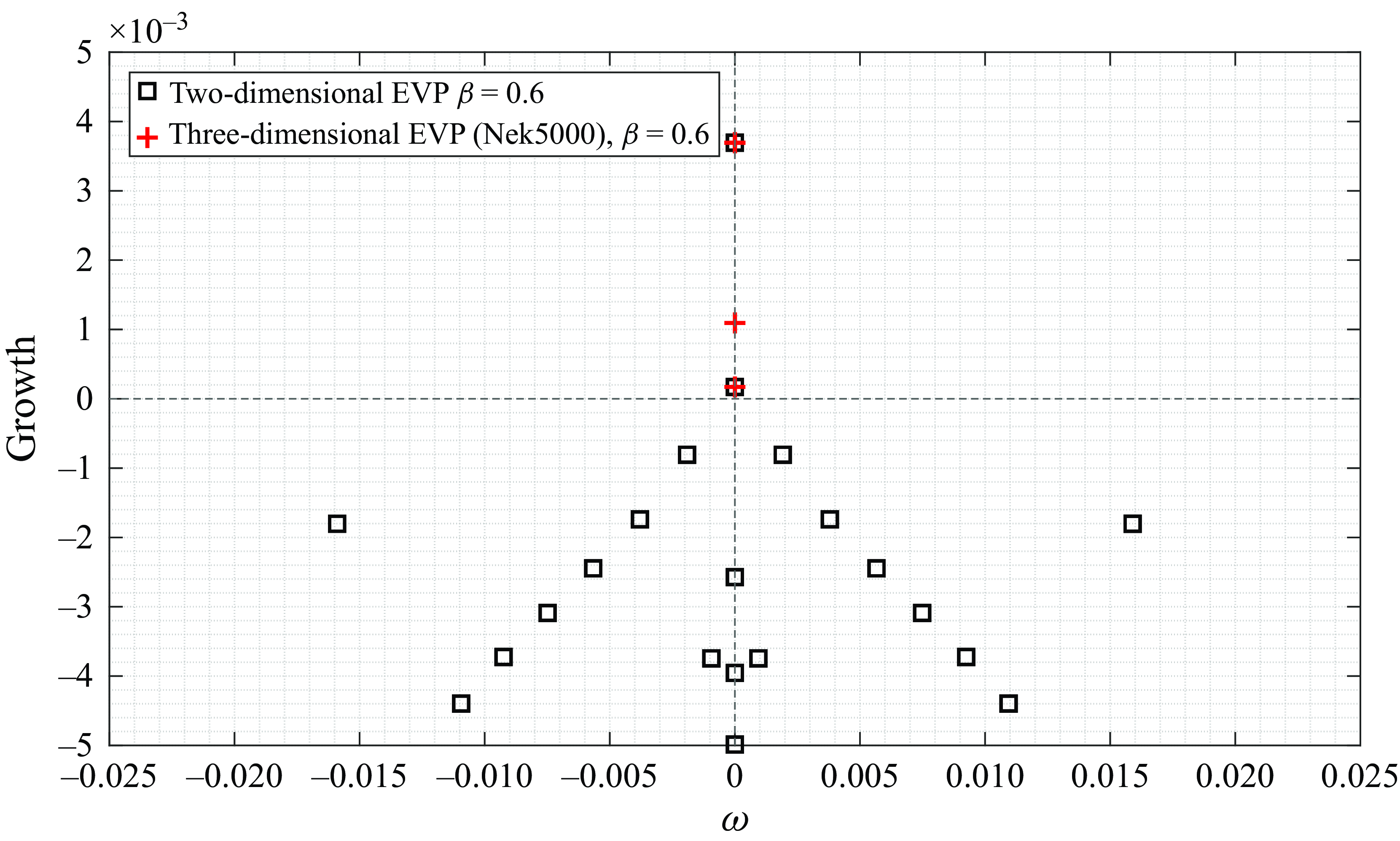
Figure 36. Eigenvalues of the two-dimensional eigenvalue problem close to the origin ( $\omega = 0$
) for case E,
$\omega = 0$
) for case E, $\beta = 0.6$
. Red plus signs show the eigenvalues obtained using Nek5000. Note that the second unstable mode obtained with Nek5000 corresponds to the first harmonic (
$\beta = 0.6$
. Red plus signs show the eigenvalues obtained using Nek5000. Note that the second unstable mode obtained with Nek5000 corresponds to the first harmonic ( $\beta =1.2$
) of the fundamental spanwise wavenumber.
$\beta =1.2$
) of the fundamental spanwise wavenumber.
To obtain the results presented in § 4.2, different domain sizes were tested, showing that a substantially smaller domain suffices to achieve convergence for three-dimensional instabilities, compared with the requirements of the convergence of two-dimensional eigenmodes. The results shown in § 4.2 correspond to a domain with height and length 50 and 500, respectively, although the same results are obtained with a smaller domain size. A grid study has also been done, and 3000 uniformly spaced discretisation points in the $x$
direction and 200 points in the
$x$
direction and 200 points in the $y$
direction with an appropriate clustering at the wall are used to compute the spectrum for different cases, although converged results were obtained with coarser grids. Note that the domain used in the DNS simulations for the laminar–turbulent transition is larger than the domain that is required to get the convergence of the eigenvalue problem.
$y$
direction with an appropriate clustering at the wall are used to compute the spectrum for different cases, although converged results were obtained with coarser grids. Note that the domain used in the DNS simulations for the laminar–turbulent transition is larger than the domain that is required to get the convergence of the eigenvalue problem.
A.3 DNS for nonlinear saturation and transition to turbulence
The domain size and spatial resolution used for different cases for nonlinear simulations are summarised in table 5. For all nonlinear simulations, the $P_N-P_{N-2}$
formulation in Nek5000, with a polynomial order equal to 7 (
$P_N-P_{N-2}$
formulation in Nek5000, with a polynomial order equal to 7 ( $P7$
) is used, except otherwise stated. The height and length of the domain for simulations of case A are 60 and 675, respectively. For case G, the height and the length are reduced to 50 and 560, respectively. To assure the accuracy of the results with respect to the size of the domain and spatial resolution, simulations corresponding to the results given in § 4.2.1 are repeated with different grid and domain sizes: for case G, the height and length of the domain are increased to 75 and 960, respectively, and a lower polynomial order (
$P7$
) is used, except otherwise stated. The height and length of the domain for simulations of case A are 60 and 675, respectively. For case G, the height and the length are reduced to 50 and 560, respectively. To assure the accuracy of the results with respect to the size of the domain and spatial resolution, simulations corresponding to the results given in § 4.2.1 are repeated with different grid and domain sizes: for case G, the height and length of the domain are increased to 75 and 960, respectively, and a lower polynomial order ( $P5$
) is used. Figure 37 compares the temporal evolution of the peak perturbation velocity in the domain for this grid (blue circles) and the reference grid (solid line) until the appearance of oscillations in the domain due to self-excited secondary instabilities.
$P5$
) is used. Figure 37 compares the temporal evolution of the peak perturbation velocity in the domain for this grid (blue circles) and the reference grid (solid line) until the appearance of oscillations in the domain due to self-excited secondary instabilities.
Table 5. Simulation parameters for nonlinear simulations. Here $N_x$
,
$N_x$
, $N_y$
and
$N_y$
and $N_z$
are the number of spectral elements in the
$N_z$
are the number of spectral elements in the $x$
,
$x$
, $y$
and
$y$
and $z$
direction, respectively. Note that each element consists of eight GLL points (seventh-order polynomial). Here
$z$
direction, respectively. Note that each element consists of eight GLL points (seventh-order polynomial). Here $L$
is the length,
$L$
is the length, $H$
is the height and
$H$
is the height and $L_z$
is the spanwise size of the simulation domain.
$L_z$
is the spanwise size of the simulation domain.
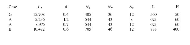
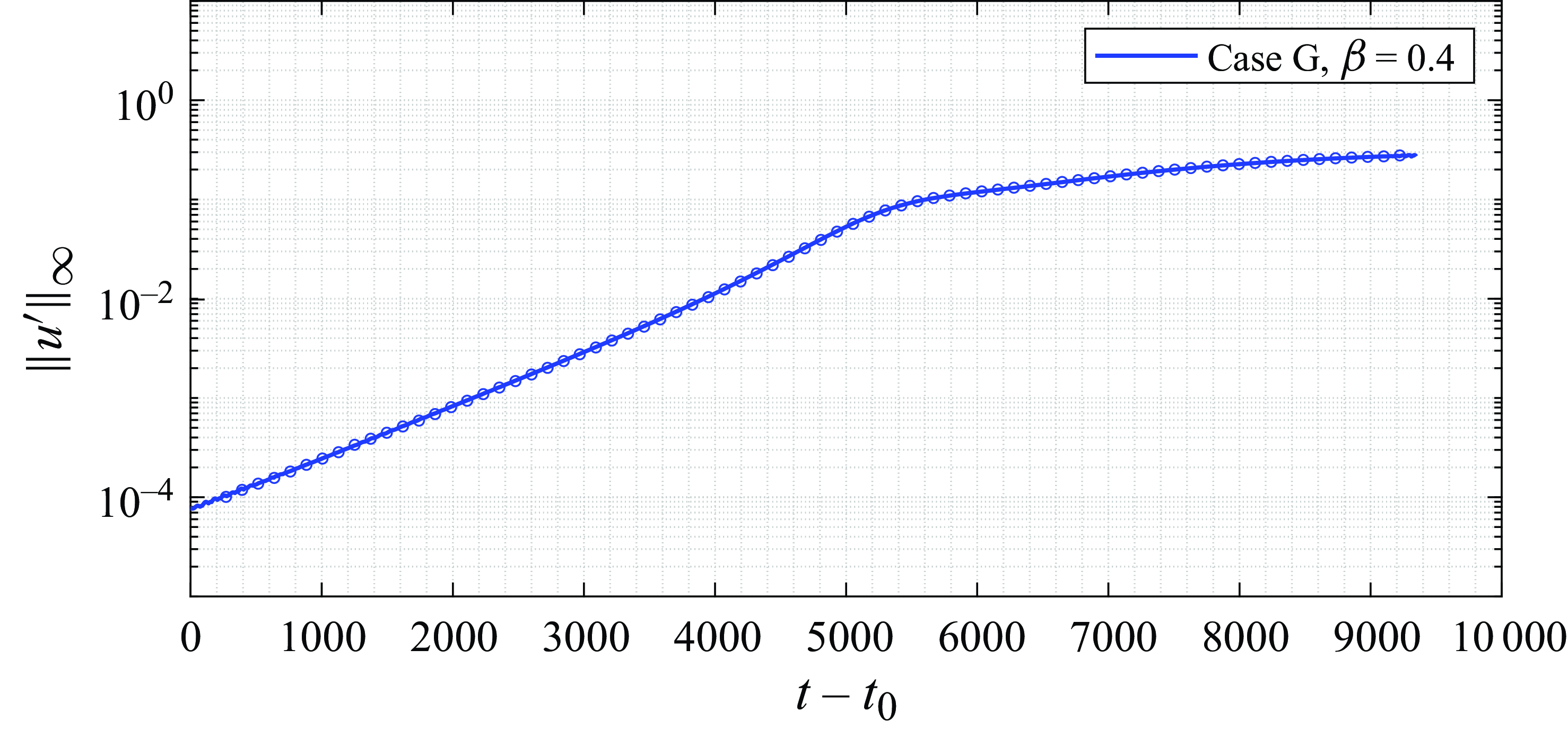
Figure 37. Time evolution of peak of the absolute value of streamwise perturbation ( $\|u'\|_{\infty }$
) for reference (solid line) and coarse (blue circles) grids. Different domain sizes are used for each simulation.
$\|u'\|_{\infty }$
) for reference (solid line) and coarse (blue circles) grids. Different domain sizes are used for each simulation.
To check the convergence of the results for case A with $\beta =1.2$
, the length and height of the domain are increased to 750 and 120, respectively, and a lower polynomial order (
$\beta =1.2$
, the length and height of the domain are increased to 750 and 120, respectively, and a lower polynomial order ( $P5$
) is used. For this simulation, the peak perturbation velocity
$P5$
) is used. For this simulation, the peak perturbation velocity $(u')$
at the saturated state differs by only 0.1 % from that for the reference grid. Using a lower polynomial order
$(u')$
at the saturated state differs by only 0.1 % from that for the reference grid. Using a lower polynomial order $(P5)$
for case A with
$(P5)$
for case A with $\beta =0.7$
changed the peak perturbation velocity at the saturated state by only 0.5 %, which shows the accuracy of the results.
$\beta =0.7$
changed the peak perturbation velocity at the saturated state by only 0.5 %, which shows the accuracy of the results.
To check the independency of the results presented in § 6.1.1 (case G, $\beta =0.4$
) with respect to domain size and grid resolution, the length of the domain was extended from 560 to 675 and the height was increased from 50 to 60. Furthermore, the resolution in all directions was increased by
$\beta =0.4$
) with respect to domain size and grid resolution, the length of the domain was extended from 560 to 675 and the height was increased from 50 to 60. Furthermore, the resolution in all directions was increased by $\approx 20 \,\%$
, which almost doubles the number of total elements in the domain compared with the reference grid. Note that the grid spacing in the
$\approx 20 \,\%$
, which almost doubles the number of total elements in the domain compared with the reference grid. Note that the grid spacing in the $x$
and
$x$
and $y$
direction are not uniform, and a finer grid resolution is used in the vicinity and downstream of the bubble. The simulation for the finer grid is restarted from the two-dimensional base flow and is continued until four complete turbulent bursts happen (see § 6.1.1). Since obtaining the saturated base flow for the finer grid is very expensive, the growth rate of the secondary instabilities for four different S phases is approximated using the kinetic energy of perturbations with respect to the initial two-dimensional base flow, and is found to be in the range
$y$
direction are not uniform, and a finer grid resolution is used in the vicinity and downstream of the bubble. The simulation for the finer grid is restarted from the two-dimensional base flow and is continued until four complete turbulent bursts happen (see § 6.1.1). Since obtaining the saturated base flow for the finer grid is very expensive, the growth rate of the secondary instabilities for four different S phases is approximated using the kinetic energy of perturbations with respect to the initial two-dimensional base flow, and is found to be in the range $[0.0132,0.0148]$
. The growth rates estimated in the same manner for the simulation using the reference grid are in the range
$[0.0132,0.0148]$
. The growth rates estimated in the same manner for the simulation using the reference grid are in the range $[0.0131,0.0151]$
. The close agreement between the growth rates assure that the reference grid is sufficient to capture the dynamics accurately. To further check the dependency of the results to grid and domain size, the time between subsequent turbulent bursts was also calculated for two grids, being
$[0.0131,0.0151]$
. The close agreement between the growth rates assure that the reference grid is sufficient to capture the dynamics accurately. To further check the dependency of the results to grid and domain size, the time between subsequent turbulent bursts was also calculated for two grids, being $[1106,1313]$
and
$[1106,1313]$
and $[1073,1378]$
for reference and finer grids, respectively.
$[1073,1378]$
for reference and finer grids, respectively.
As shown in Appendix A.1, the growth of the two-dimensional global mode is very sensitive to the size of the domain. Thus, for simulations corresponding to § 6.2 (case E, $\beta =0.6$
), the height and length of the domain are chosen as
$\beta =0.6$
), the height and length of the domain are chosen as $H=400$
and
$H=400$
and $L=788$
, respectively, to capture the two unstable two-dimensional global modes as shown in § 4. The number of spectral elements used for this simulation in each direction is
$L=788$
, respectively, to capture the two unstable two-dimensional global modes as shown in § 4. The number of spectral elements used for this simulation in each direction is $(N_x,N_y,N_z)=(705,46,12)$
, which results in 524520
$(N_x,N_y,N_z)=(705,46,12)$
, which results in 524520 $(P7)$
total elements (
$(P7)$
total elements ( $\approx 269$
million grid points).
$\approx 269$
million grid points).
Appendix B. Construction of perturbation field for impulse response analysis
The localised initial perturbation field used in § 5.2 is by imposing an analytic $v$
velocity field as follows. First, the impulse field
$v$
velocity field as follows. First, the impulse field $(IF)$
in each Cartesian direction is defined as
$(IF)$
in each Cartesian direction is defined as
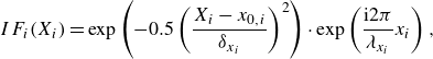 \begin{equation} IF_{i}(X_i)=\exp \left (-0.5\left (\frac {X_i-x_{0,i}}{\delta _{x_i}}\right )^2 \right ) \cdot \exp \left ({\frac {\mathrm{i}2\pi }{\lambda _{x_i}}x_i}\right ), \end{equation}
where $i=(1,2,3)$
,
$i=(1,2,3)$
, $(x_1,x_2,x_3)=(x,y,z)$
and
$(x_1,x_2,x_3)=(x,y,z)$
and $X_i$
is the vector of grid coordinates. The parameters
$X_i$
is the vector of grid coordinates. The parameters $\delta _{x_i}$
and
$\delta _{x_i}$
and $\lambda _{x_i}$
control the width and wavelength of the perturbations centred at
$\lambda _{x_i}$
control the width and wavelength of the perturbations centred at $x_{0,i}$
, respectively. The perturbation field is then taken as
$x_{0,i}$
, respectively. The perturbation field is then taken as
 \begin{equation} IF=\epsilon \cdot Re [IF_1 \cdot IF_2 \cdot (IF_{3,p}+IF_{3,n})], \end{equation}
where $\epsilon$
is a small amplitude. The same
$\epsilon$
is a small amplitude. The same $\delta _{x_3}$
and
$\delta _{x_3}$
and $x_{0,3}$
is used for
$x_{0,3}$
is used for $IF_{3,p}$
and
$IF_{3,p}$
and $IF_{3,n}$
; however, positive and negative
$IF_{3,n}$
; however, positive and negative $\lambda _{x_3}$
(with the same magnitude) are used for
$\lambda _{x_3}$
(with the same magnitude) are used for $IF_{3,p}$
and
$IF_{3,p}$
and $IF_{3,n}$
, respectively. The resulting field is then projected onto a divergence free space and applied as the initial condition.
$IF_{3,n}$
, respectively. The resulting field is then projected onto a divergence free space and applied as the initial condition.


 Open access