


1. Introduction
Calculating the shape of a sessile drop on a horizontal substrate is a classical hydrostatic problem (Finn Reference Finn1986). Its understanding is a prerequisite to both more complicated static drop configurations (Concus Reference Concus1968; Concus & Finn Reference Concus and Finn1969) and the transition to drop motion on substrates (Dussan V. Reference Dussan V.1979; Hodges, Jensen & Rallison Reference Hodges, Jensen and Rallison2004). Owing to axial symmetry, the interfacial force balance normal to the drop interface may be written as an ordinary differential equation. The complete mathematical problem governing the drop shape consists of that equation together with appropriate subsidiary conditions. The dimensionless problem involves only two parameters. The first is the contact angle  $\alpha$, specified at the contact line. The second is the Bond number $B$, which enters through the interfacial force balance; it represents the ratio of gravitational to capillary forces.
No closed-form solution exists for arbitrary  $B$ and $\alpha$ (Finn Reference Finn1986). The extreme limits of small and large $B$, which provide approximate descriptions, are therefore of interest. In the limit $B\to 0$, wherein gravity is negligible, the drop shape is a spherical cap (Chesters Reference Chesters1977; Shanahan Reference Shanahan1984; Smith & Van de Ven Reference Smith and Van de Ven1984; Quéré, Azzopardi & Delattre Reference Quéré, Azzopardi and Delattre1998). This limit is regular, except for the case of a non-wetting drop ( $\alpha ={\rm \pi}$) where the flat-spot region near the contact line must be addressed separately (Mahadevan & Pomeau Reference Mahadevan and Pomeau1999; Hodges et al. Reference Hodges, Jensen and Rallison2004; Schnitzer, Davis & Yariv Reference Schnitzer, Davis and Yariv2020).
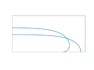
In the other extreme,  $B\to \infty$, gravity is dominant. The drop adopts a pancake-like shape where surface tension is negligible except near the edge, see figure 1. This problem, originally addressed by Laplace (Reference Laplace1805) and Rayleigh (Reference Rayleigh1916), constitutes a classical example of a boundary-layer configuration (Rienstra Reference Rienstra1990; Van Dyke Reference Van Dyke1994). When formulating the problem in a manner which reflects experimental protocol, the drop volume is specified (Quéré et al. Reference Quéré, Azzopardi and Delattre1998; Aussillous & Quéré Reference Aussillous and Quéré2006). Using that approach, Quéré and coworkers addressed the pancake limit using two different derivations. The first is a ‘mechanical’ one (De Gennes, Brochard-Wyart & Quéré Reference De Gennes, Brochard-Wyart and Quéré2003), using an approximate radial force balance on the drop edge. The second (Quéré Reference Quéré2005) uses an energetic approach, where the constraint of a specified volume was handled using Lagrange multipliers. In both approaches, the authors obtain approximations for the pancake shape parameters (radius and height) without solving any differential equations.

Figure 1. Numerically evaluated drop shape for  $\alpha ={\rm \pi}$ and $\alpha ={\rm \pi} /2$, generated using the scheme of § 6; (a) $B=1$ and (b) $B=10$.
It is desirable to devise a systematic scheme for the large- $B$ limit which, on one hand, would shed light upon the above-mentioned approximations, and, on the other hand, would allow for the possibility of going beyond them to any asymptotic order. The large- $B$ limit was analysed by Rienstra (Reference Rienstra1990) using asymptotic terminology and notation. Reinstra's analysis, however, is based on a formulation where contact angle and drop volume are not prescribed quantities, resulting in an analysis that ultimately provides explicit results only to leading order. Moreover, Reinstra's analysis relies on direct solution of the governing differential equations, whereas the mechanistic approach in De Gennes et al. (Reference De Gennes, Brochard-Wyart and Quéré2003) suggests that integral balances may provide valuable simplifications.
Our goal here is to revisit the pancake limit  $B\gg 1$ using a contemporary formulation where the drop volume is specified. In particular, we shall employ the method of matched asymptotic expansions (Hinch Reference Hinch1991), natural for handling this singular limit, to systematically derive asymptotic approximations of the pancake shape parameters, going beyond known leading-order results. Motivated by the mechanistic approach in De Gennes et al. (Reference De Gennes, Brochard-Wyart and Quéré2003), we shall employ two integral-force balances in order to simplify our analysis: a familiar vertical balance and a second, newly derived, balance that we shall be able to interpret as a generalisation of the intuitive leading-order radial balance used in De Gennes et al. (Reference De Gennes, Brochard-Wyart and Quéré2003).
The paper is arranged as follows. In the next section, we formulate the hydrostatic problem and derive the vertical force balance. In § 3 we discuss the meniscus parameterisation and derive the generalised radial balance mentioned above. In § 4 we deduce scalings and leading-order approximations for the pancake shape parameters. Facilitated by the distinction between algebraically and exponentially small terms, the asymptotic analysis in the limit  $B\to \infty$ is carried out in § 5. A numerical scheme for solving the exact problem, tailored to large values of $B$, is introduced in § 6. An approximation of the exponentially small apex pressure, required for the application of that scheme at these values, is obtained in § 7 using a Wentzel–Kramers–Brillouin (WKB) method. In § 8 we compare the large- $B$ asymptotic approximations with the numerical calculations. The large- $B$ limit of the comparable two-dimensional problem is discussed in § 9. We conclude at § 10.
2. Problem formulation
A drop of density  $\rho$ and surface tension $\gamma$ rests on a horizontal substrate. The drop volume is $4{\rm \pi} a^3/3$. The contact angle is $\alpha$. In formulating a dimensionless problem, we adopt a convention where lengths are normalised by $a$ and pressure by $\gamma /a$. We employ cylindrical $(r,\theta,z)$ coordinates, $r=0$ being the symmetry axis and the plane $z=0$ at the substrate. The contact-line radius is denoted by $r^*$. The height of the free surface at the symmetry axis is denoted by $z^*$.
The pressure field within the drop is given by
 \begin{equation} p = p^*-Bz, \end{equation}
where  $p^*$ is the (as yet unknown) pressure at $z=0$ and $B=\rho g a^2/\gamma$ is the Bond number, representing the ratio of gravity to capillarity. This number may be written as the ratio of length scales
 \begin{equation} B = (a/l)^2, \end{equation}
in which the capillary length  $l$ is defined by
 \begin{equation} l^2 = \frac{\gamma}{\rho g} . \end{equation}
Using (2.1), the Young–Laplace equation condition at the free surface reads
 \begin{equation} p^*-Bz = \boldsymbol{\nabla}\boldsymbol{\cdot}\hat{\boldsymbol{n}}, \end{equation}
wherein  $\hat {\boldsymbol {n}}$ in an outward-pointing unit vector normal to the surface. This equation is supplemented by the volume constraint
 \begin{equation} \text{drop volume} = \frac{4{\rm \pi}}{3}, \end{equation}
together with the prescription of a contact angle  $\alpha$,
 \begin{equation} \hat{\boldsymbol{n}} = \hat{\boldsymbol{e}}_r \sin\alpha+ \hat{\boldsymbol{e}}_z\cos\alpha, \quad \text{at} \ z=0. \end{equation}
Defining the unit vector  $\hat {\boldsymbol {m}} = \hat {\boldsymbol {e}}_\theta \times \hat {\boldsymbol {n}}$, we have
 \begin{equation} \hat{\boldsymbol{m}} = \hat{\boldsymbol{e}}_r \cos\alpha-\hat{\boldsymbol{e}}_z\sin\alpha, \quad \text{at} \ z=0. \end{equation}
That vector is tangential to the meniscus and perpendicular to the contact line.
In what follows, it is convenient to employ an integral-force balance (with forces normalised by  $\gamma a$). Considering the drop together with the meniscus, that balance involves the pressure force at the substrate, $\hat {\boldsymbol {e}}_z {\rm \pi}{r^*}^2 p^*$, the drop weight $-\hat {\boldsymbol {e}}_z (4{\rm \pi} /3)B$ (recall (2.5)), and the surface tension, provided by the integral of $\hat {\boldsymbol {m}}$ over the contact circle (of length $2{\rm \pi} r^*$). We therefore obtain using (2.7)
 \begin{equation} p^*{r^*}^2 = \frac{4B}{3} + 2r^* \sin\alpha. \end{equation}
While condition (2.8) does not provide any independent information, it may serve as a convenient alternative to (2.5).
For future reference, we note that the apex pressure is
 \begin{equation} p^{**} = p^* - Bz^*. \end{equation}
3. Shape parametrisation
Following Rienstra (Reference Rienstra1990) we employ parametrisation in the meridian plane using the arclength  $s$ measured from the detachment point. The free surface is described using the local inclination angle $\phi$, whereby the outward unit vector normal to the surface is
 \begin{equation} \hat{\boldsymbol{n}}=\hat{\boldsymbol{e}}_r \sin\phi-\hat{\boldsymbol{e}}_z\cos\phi. \end{equation}
The associated curvature is  $\boldsymbol {\nabla }\boldsymbol {\cdot }\hat {\boldsymbol {n}}=\mathrm {d}\phi /\mathrm {d} s + r^{-1}\sin \phi$. The Young–Laplace equation (2.4) then gives
 \begin{equation} \frac{\mathrm{d}{\phi}}{\mathrm{d}{s}} + \frac{\sin\phi}{r} = p^*-Bz. \end{equation}
Regarding  $r$ and $z$ as functions of $s$, they are governed by the differential equations
 \begin{equation} \frac{\mathrm{d}{r}}{\mathrm{d}{s}} = \cos\phi, \quad \frac{\mathrm{d}{z}}{\mathrm{d}{s}} = \sin\phi. \end{equation}
These first-order equations are supplemented by the ‘initial’ conditions
 \begin{equation} r(0) = r^*, \quad z(0)=0 , \end{equation}
as well as the contact-angle condition (cf. (2.6))
 \begin{equation} \phi(0)={\rm \pi}-\alpha. \end{equation}
The arclength  $s$ ranges between $0$ and $s_{M}$, wherein the maximal value $s_{M}$ is set by the condition $\phi (s_{M})={\rm \pi}$. The two parameters in the problem, $p^*$ and $r^*$, are to be determined from the volume constraint (cf. (2.5)),
 \begin{equation} \int_0^{s_{M}}r^2\frac{\mathrm{d}{z}}{\mathrm{d}{s}} \, \mathrm{d} s = \frac{4}{3}, \end{equation}
and the symmetry condition,
 \begin{equation} r(s_{M})=0. \end{equation}
 In the analysis that follows it is preferable to employ  $\phi$ as the independent variable (running from ${\rm \pi} -\alpha$ to ${\rm \pi}$) instead of $s$. With a slight abuse of notation, equations (3.2)–(3.3) are then replaced by
 \begin{equation} \frac{\mathrm{d}{r}}{\mathrm{d}{\phi}} = \frac{r\cos\phi}{p^*r-Brz-\sin\phi}, \quad \frac{\mathrm{d}{z}}{\mathrm{d}{\phi}} = \frac{r\sin\phi}{p^*r-Brz-\sin\phi}, \end{equation}
while conditions (3.4) become
 \begin{equation} r({\rm \pi}-\alpha) = r^*, \quad z({\rm \pi}-\alpha)=0 . \end{equation}
The volume constraint (3.6) now reads
 \begin{equation} \int_{{\rm \pi}-\alpha}^{\rm \pi} r^2 \frac{\mathrm{d}{z}}{\mathrm{d}{\phi}} \, \mathrm{d} \phi = \frac{4}{3}, \end{equation}
while the symmetry condition (3.7) becomes
 \begin{equation} r({\rm \pi})=0. \end{equation}
In that formulation, the drop height is obtained as
 \begin{equation} z^* = z({\rm \pi}). \end{equation}
A useful integral equation may be obtained as follows. We write (3.8b) in the form
 \begin{equation} (p^*-Bz)\, \mathrm{d} z - \frac{\sin\phi}{r} \frac{\mathrm{d}{z}}{\mathrm{d}{\phi}} \, \mathrm{d}\phi = \sin\phi \, \mathrm{d}\phi, \end{equation}
and integrate over  $\phi$ from ${\rm \pi} -\alpha$ to ${\rm \pi}$, which implies integration over $z$ from $0$ to $z^*$ (see (3.9b) and (3.12)). This gives
 \begin{equation} p^*z^* - \frac{B{z^*}^2}{2} - \int_{{\rm \pi}-\alpha}^{\rm \pi} \frac{\sin\phi}{r} \frac{\mathrm{d}{z}}{\mathrm{d}{\phi}} \, \mathrm{d}\phi = 1 - \cos\alpha. \end{equation}
4. Scalings and pancake size as  $B\to \infty$

For given  $\alpha$ and $B$, the problem formulation of § 2 defines the base pressure $p^*$ and the shape – in particular $r^*$ and $z^*$. There is no closed-form analytic solution to that problem (Finn Reference Finn1986). Our interest lies in the limit of large drops, where $B$ is large. With gravity being dominant, it is evident that the drop adopts an approximate pancake shape, with the radius being approximately $r^*$ and the uniform height being approximately $z^*$. In this section, we intend to find the scaling of these shape parameters, and then evaluate them (approximately) without solving any differential equations.
We begin with scaling arguments. It is evident from the volume constraint (2.5) that  ${r^*}^2z^*=\operatorname {ord}(1)$. From the Young–Laplace balance (2.4) we see that $p^* = \operatorname {ord}(Bz^*)$. Since the latter relation involves the unknown $p^*$ we need another scaling law. To that end, consider the edge region about the rim. In that region the shape is independent at leading order of the drop volume. Since the only pertinent length scale is then the capillary length $l$ (recall (2.3)), it follows that (see (2.2))
 \begin{equation} z^* = \operatorname{ord}(B^{{-}1/2}). \end{equation}
Consequently, we have
 \begin{equation} r^* = \operatorname{ord}(B^{1/4}), \quad p^* = \operatorname{ord}(B^{1/2}). \end{equation}
We can now go beyond scaling, obtaining three approximations governing the above quantities. The first follows from the volume constraint (2.5), which gives here
 \begin{equation} {r^*}^2 z^* \approx \tfrac{4}{3}. \end{equation}
The second is the Young–Laplace balance (2.4), which, when applied to the flat portion of the pancake shape, gives
 \begin{equation} p^* \approx Bz^*. \end{equation}
The third is derived from the integral relation (3.14). It follows from (4.1)–(4.2) that the integral term in (3.14) is subdominant to the  $\operatorname {ord}(1)$ terms. We therefore obtain
 \begin{equation} p^*z^* - \frac{B{z^*}^2}{2} \approx 1 - \cos\alpha. \end{equation}
The solution of (4.3)–(4.5) is
 \begin{equation} p^* \approx B^{1/2} \varPi_0, \quad z^* \approx B^{{-}1/2} \varPi_0, \quad r^* \approx B^{1/4} {R}^*_0, \end{equation}
wherein
 \begin{equation} \varPi_0 = 2 \sin\frac{\alpha}{2}, \quad {R}^*_0 = \sqrt{\frac{2}{3\sin(\alpha/2)}}. \end{equation}
These constitute the dimensionless counterparts of results obtained in De Gennes et al. (Reference De Gennes, Brochard-Wyart and Quéré2003) and Quéré (Reference Quéré2005). Note that the force balance (2.8) is trivially satisfied at leading order, with the last term subdominant. This is consistent with our comment following (2.8) regarding independence.
It is interesting to note that De Gennes et al. (Reference De Gennes, Brochard-Wyart and Quéré2003) use (see their (2.7) and their figure 2.4) a dimensional version of (4.5), which presumably expresses ‘equilibrium of the forces (per unit length of the line of contact).’ De Gennes et al. (Reference De Gennes, Brochard-Wyart and Quéré2003) do not explain the nature of approximation in their equation (2.7). (With the contact-line curvature in the azimuthal direction being ignored, it is not an exact balance.) In contrast to the intuitive approach in De Gennes et al. (Reference De Gennes, Brochard-Wyart and Quéré2003), here we have obtained (4.5) by approximating the exact integral balance (3.14). As will become evident, that exact condition can be interpreted in the limit  $B\to \infty$ as an ‘edge balance’, up to exponentially small terms, with (4.5) emerging at leading order.
It is also worth noting that the approximate relation (4.5) may be obtained using a different approach. As in the derivation of (2.8), we employ an integral force balance on the drop together with its meniscus. Here, however, we consider half of the drop, applying the force balance in a direction perpendicular to a mid-plane. Since gravity does not contribute in that direction, we have a balance between pressure force on the mid-plane and surface-tension forces. In the pancake approximation, the pressure force is approximately given by
 \begin{equation} 2r^* \int_0^{z^*} p(z)\, \mathrm{d} z. \end{equation}
It is opposed by surface tension at the ‘top’ flat meniscus,  $\approx 2r^*$, and supplemented by surface-tension forces at the contact line which, when projected perpendicular to mid-plane, approximately sum up to $2r^*\cos \alpha$ (recall (2.7)). We therefore have
 \begin{equation} \int_0^{z^*} p(z)\, \mathrm{d} z \approx 1-\cos\alpha. \end{equation}
Plugging in (2.1) gives (4.5). The derivation of an exact force balance over half the drop, is, however, not as straightforward. We therefore prefer to employ the exact relation (3.14), which is later used beyond leading order.
5. Asymptotic analysis in the limit $B\to \infty$

In what follows we proceed with a systematic asymptotic calculation, perturbing about (4.6)–(4.7). This allows us to improve upon the approximation originally obtained by Quéré and coworkers. The analysis is facilitated by the conceptual decomposition of the drop domain into a ‘flat region’, where capillarity is negligible, and an ‘edge region’, close to the contact line, where capillarity play a dominant role.
5.1. Rescaling
Motivated by (4.6), we introduce rescaled quantities
 \begin{equation} p^* = B^{1/2} \varPi, \quad z^* = B^{{-}1/2} Z^*, \quad r^* = B^{1/4} {R}^*. \end{equation}
These satisfy
 \begin{equation} \lim_{B\to\infty} \varPi = \varPi_0, \quad \lim_{B\to\infty} Z^* = \varPi_0, \quad \lim_{B\to\infty} {R}^* = {R}^*_0, \end{equation}
wherein  $\varPi _0$ and ${R}^*_0$ are given by (4.7). In terms of the rescaled quantities, the pressure field (2.1) reads
 \begin{equation} p = B^{1/2}(\varPi-Z), \end{equation}
with the apex pressure (2.9) becoming
 \begin{equation} p^{**} = B^{1/2}(\varPi-Z^*), \end{equation}
and the vertical force balance (2.8) reading
 \begin{equation} {{R}^*}^2 \varPi = \tfrac{4}{3} + 2B^{{-}3/4} {R}^* \sin\alpha. \end{equation}
 Similarly to (5.1b,c), we also define the associated stretched coordinates  $Z$ and $R$ as
 \begin{equation} z=B^{{-}1/2}Z, \quad r=B^{1/4}{R} . \end{equation}
5.2. Exponentially small terms
In terms of the rescaled quantities, the Young–Laplace balance (2.4) becomes
 \begin{equation} \varPi - Z = B^{{-}1/2} \boldsymbol{\nabla}\boldsymbol{\cdot}\hat{\boldsymbol{n}}. \end{equation}
In the flat region we can write the shape as
 \begin{equation} Z=\varPi + G({R}). \end{equation}
We claim that  $G$ is exponentially small in that region. Indeed, with $Z$ being uniform at leading order, $\boldsymbol {\nabla }\boldsymbol {\cdot }\hat {\boldsymbol {n}}$ vanishes, so does not provide a correction term in (5.7) at any algebraic order.
In particular, we note that
 \begin{equation} Z^* = \varPi+ G(0), \end{equation}
that is,
 \begin{equation} Z^* = \varPi+ \text{exponentially small terms}. \end{equation}
Neglecting such terms we may replace  $Z^*$ by $\varPi$, reducing the number of parameters.
With height variations being exponentially small in the flat region, it is clear that the contribution from that region to the integral in the balance (3.14) is also exponentially small. That integral is therefore dominated by the edge region at all algebraic orders and thence (3.14) can be interpreted as an edge balance.
5.3. The edge region
We have already observed that the extent of edge region is  $\operatorname {ord}(B^{-1/2})$. The stretched coordinate $Z$, as defined in (5.6), is therefore appropriate for that region too. The appropriate stretched coordinate X in the radial direction is defined via
 \begin{equation} r = B^{1/4} {R}^* + B^{{-}1/2} X, \end{equation}
or, using (5.6b),
 \begin{equation} {R} = {R}^* + B^{{-}3/4} X. \end{equation}
With a slight abuse of notation, the edge shape is written as
 \begin{equation} X=X(\phi), \quad Z = Z(\phi), \end{equation}
whereby (5.12) provides the parametric form
 \begin{equation} {R} = {R}^* + B^{{-}3/4} X(\phi). \end{equation}
Equations (3.8) become
 \begin{equation} \frac{\mathrm{d}{X}}{\mathrm{d}{\phi}} = \frac{\cos\phi}{\varPi-Z-B^{{-}3/4}{R}^{{-}1}\sin\phi}, \quad \frac{\mathrm{d}{Z}}{\mathrm{d}{\phi}} = \frac{\sin\phi}{\varPi-Z-B^{{-}3/4}{R}^{{-}1}\sin\phi}, \end{equation}
with  ${R}$ provided by (5.14), while conditions (3.9) now read
 \begin{equation} X({\rm \pi}-\alpha) =0, \quad Z({\rm \pi}-\alpha) = 0. \end{equation}
Last, making use of (5.10), the integral relation (3.14) is simplified to
 \begin{equation} \frac{{\varPi}^2}{2} - B^{{-}3/4}\int_{{\rm \pi}-\alpha}^{\rm \pi} \frac{\sin\phi}{R} \frac{\mathrm{d}{Z}}{\mathrm{d}{\phi}} \, \mathrm{d}\phi = 1 - \cos\alpha, \end{equation}
with an exponentially small error. As in (5.15),  ${R}$ is provided by (5.14).
5.4. Asymptotic expansions
Both the vertical force balance (5.5) and the edge balance (5.17) imply asymptotic correction of relative magnitude  $O(B^{-3/4})$ to the limiting values (5.2). (That magnitude is also suggested by (5.15).) Given (5.10), we only need to deal with two parameters. We therefore write
 \begin{equation} \varPi = \varPi_0 + B^{{-}3/4} \varPi_1 + \cdots, \quad {R}^* = {R}^*_0 + B^{{-}3/4} {R}^*_1 + \cdots. \end{equation}
We therefore employ the expansions
 \begin{equation} X = X_0(\phi) + B^{{-}3/4} X_1(\phi) + \cdots, \quad Z = Z_0(\phi) + B^{{-}3/4}Z_1(\phi) + \cdots. \end{equation}
Note that (5.14) gives
 \begin{equation} {R} = {R}^*_0 + B^{{-}3/4} \left[ {R}^*_1 + X_0(\phi)\right] + \cdots. \end{equation}
 Our goal is the calculation of the leading-order corrections  $\varPi _1$ and ${R}^*_1$. The requisite two equations are obtained from the integral balances at $\operatorname {ord}(B^{-3/4})$. Thus, from the vertical balance (5.5) we find
 \begin{equation} {R}^*_0 \varPi_1 + 2\varPi_0{R}^*_1 = 2\sin\alpha, \end{equation}
while from the radial balance (5.17) we obtain, using (5.20),
 \begin{equation} \varPi_0\varPi_1 = \frac{1}{{R}^*_0} \int_{{\rm \pi}-\alpha}^{\rm \pi} \frac{\mathrm{d}{Z_0}}{\mathrm{d}{\phi}} \sin\phi \, \mathrm{d}\phi . \end{equation}
To obtain  $Z_0(\phi )$ we need to explicitly consider the edge region.
5.5. Leading-order edge shape
At leading order, (5.15) becomes
 \begin{equation} \frac{\mathrm{d}{X_0}}{\mathrm{d}{\phi}} = \frac{\cos\phi}{\varPi_0-Z_0}, \quad\frac{\mathrm{d}{Z_0}}{\mathrm{d}{\phi}} = \frac{\sin\phi}{\varPi_0-Z_0} , \end{equation}
while conditions (5.16) give
 \begin{equation} X_0({\rm \pi}-\alpha) =0, \quad Z_0({\rm \pi}-\alpha) = 0. \end{equation}
Using (4.7a) we readily find the solution of (5.23b) and (5.24b)
 \begin{equation} Z_0 = \varPi_0 - 2\cos\frac{\phi}{2}. \end{equation}
As  $\phi \to {\rm \pi}$, $Z_0\to \varPi _0$, in agreement with the expected approach to the pancake flatness (5.10). In particular, we obtain from (5.25):
 \begin{equation} Z_0 = \varPi_0 - ({\rm \pi}-\phi) +o({\rm \pi}-\phi) ,\quad \text{as} \ \phi\to{\rm \pi}. \end{equation}
Substituting (5.25) into (5.23a) yields, using (5.24a),
 \begin{equation} X_0 = 2 \sin\frac{\phi}{2} - \operatorname{arctanh} \sin\frac{\phi}{2} - 2 \cos\frac{\alpha}{2} + \operatorname{arctanh} \cos\frac{\alpha}{2} . \end{equation}
As expected,  $X_0\to -\infty$ as $\phi \to {\rm \pi}$. The approach is logarithmically slow; thus
 \begin{equation} X_0 \sim{-}\ln\frac{4}{{\rm \pi}-\phi} + 4\sin^2\frac{\alpha}{4} + \operatorname{arctanh} \cos\frac{\alpha}{2} ,\quad \text{as} \ \phi\to{\rm \pi}, \end{equation}
where the asymptotic error is algebraically small in  ${\rm \pi} -\phi$.
For  $\phi >{\rm \pi} /2$ the meniscus shape may be written in the form
 \begin{equation} Z_0 = H(X_0). \end{equation}
In what follows, we require the behaviour of  $H$ as $X_0\to -\infty$. Substituting (5.28) into (5.26) yields
 \begin{equation} H(X_0) \sim \varPi_0 -4\exp\left( X_0-4\sin^2\frac{\alpha}{4}-\operatorname{arctanh} \cos\frac{\alpha}{2}\right) ,\quad \text{as} \ X_0\to-\infty. \end{equation}
Note the exponential approach to the flat-region height  $\varPi _0$.
5.6. Leading-order shape corrections
Having calculated  $Z_0(\phi )$, we can obtain the shape corrections. Substituting (5.25) into (5.22) gives, upon making use of (4.7),
 \begin{equation} \varPi_1 = \left(\frac{2}{3}\right)^{1/2} \frac{1-\cos^3(\alpha/2)}{\sin^{1/2}(\alpha/2)}, \end{equation}
which is positive for all contact angles. From (5.21) we then obtain
 \begin{equation} {R}^*_1 = \frac{5}{6} \cos\frac{\alpha}{2} - \frac{1}{12}\sec^2\frac{\alpha}{4}. \end{equation}
It is positive for  $0<\alpha <\tilde {\alpha } {\rm \pi}$ and negative for $\tilde {\alpha } {\rm \pi}<\alpha <{\rm \pi}$, where $\tilde {\alpha }\approx 0.89$.
Recalling (5.10), we have obtained the leading-order corrections to the rescaled shape parameters  $Z^*$ and ${R}^*$. In obtaining these corrections we have used the integral balances (5.5) and (5.17) at $\operatorname {ord}(B^{-3/4})$, and the edge shape at leading order. We did not use the volume constraint (2.5). It may appear that constraint (2.5) at $\operatorname {ord}(B^{-3/4})$ in conjunction with the leading edge solution (5.25) and (5.27) may be used as an alternative equation for obtaining $\varPi _1$ and ${R}^*_1$. In Appendix A we show that the volume constraint (2.5) is trivially satisfied at $\operatorname {ord}(B^{-3/4})$. This, of course, was to be expected given the dependency between (2.5) and (2.8).
6. Numerical scheme
It is clear that  $\mathrm {d} r/\mathrm {d} \phi$ is large in the flat region, where $\phi$ is approximately constant. It follows that (3.8) become numerically challenging in the limit $B\to \infty$. In constructing a numerical scheme appropriate for that limit, it is therefore more convenient to employ the more primitive formulation (3.2)–(3.7).
We actually employ a variant of that formulation, which allows us to reduce the number of parameters. Thus, we set the origin at apex, with an axial axis  $\bar z$ pointing downwards
 \begin{equation} \bar z = z^* - z. \end{equation}
The local inclination angle is now  $\bar \phi ={\rm \pi} -\phi$. It starts at the zero value at the apex, where $\bar z = 0$, and reaches the contact angle at the substrate, where $\bar z = z^*$. We denote the arclength, as measured from the apex, by $\bar s$.
In terms of the new variables, (3.2) becomes
 \begin{equation} \frac{\mathrm{d}{\bar\phi}}{\mathrm{d}{\bar s}} + \frac{\sin\bar\phi}{r} = p^{**}+B\bar z, \end{equation}
wherein  $p^{**}$ is the apex pressure (2.9). Upon replacing $s$,
$s$,  $z$ and $\phi$ by $\bar s$, $\bar z$ and $\bar \phi$, (3.3) remains intact,
 \begin{equation} \frac{\mathrm{d}{r}}{\mathrm{d}{\bar s}} = \cos\bar\phi, \quad \frac{\mathrm{d}{\bar z}}{\mathrm{d}{\bar s}} = \sin\bar\phi, \end{equation}
while the initial conditions (3.4)–(3.5) become
 \begin{equation} r(0) = 0, \quad \bar z(0)=0 , \quad \bar\phi(0)=0. \end{equation}
The arclength  $\bar s$ ranges between $0$ and $s_{M}$, wherein now the maximal value $s_{M}$ is obtained by the condition $\bar \phi (s_{M})=\alpha$.
In the above description,  $r^*$ no longer appears in the problem formulation, so the only remaining parameter is $p^{**}$. It is determined from the volume constraint (cf. (3.6))
 \begin{equation} \int_0^{s_{M}}r^2\frac{\mathrm{d}{z}}{\mathrm{d}{\bar s}} \, \mathrm{d} \bar s = \frac{4}{3}. \end{equation}
 In implementing the above numerically, we observe that the second term in (6.2) becomes indefinite at  $\bar s=0$. Taylor expansion in conjunction with (3.3a) readily yields
 \begin{equation} \frac{\mathrm{d}{\bar\phi}}{\mathrm{d}{\bar s}} = \frac{p^{**}}{2} \quad \text{at} \ \bar s=0, \end{equation}
which replaces (6.2) at the initial step ( $\bar s=0$).
For given values of  $B$ and $\alpha$, the numerical scheme is as follows. Using an initial guess for $p^{**}$, the initial-value problem (6.2)–(6.4) is integrated until $\bar \phi$ reaches the value $\alpha$. The violation in the volume constraint (6.5) is then used to iterate for $p^{**}$. This scheme works for arbitrary values of $B$, but becomes sensitive to the initial guess for $p^{**}$ when $B$ becomes large. This is hardly surprising: given (5.4) and (5.9)–(5.10), the apex pressure,
 \begin{equation} p^{**} ={-}B^{1/2} G(0), \end{equation}
is exponentially small. It is therefore desirable to obtain an asymptotic approximation for  $p^{**}$ (or, equivalently, for the apex curvature) in the pancake limit. The exponentially small curvature profile in the flat region can be obtained using the WKB method. This is carried out in the following section, resulting in an explicit approximation for $p^{**}$.
7. Exponentially small apex curvature
Recalling that  $p^{**}$ is given by (6.7), we need an approximation for $G(R)$. Linearising the expression for curvature in cylindrical coordinates (Pozrikidis Reference Pozrikidis2011) and making use of (5.8) yields
 \begin{equation} \boldsymbol{\nabla}\boldsymbol{\cdot}\hat{\boldsymbol{n}} ={-}B^{{-}1} \left(\frac{\mathrm{d}{^2G}}{\mathrm{d}{{R}^2}} + \frac{1}{R}\frac{\mathrm{d}{G}}{\mathrm{d}{R}}\right), \end{equation}
with errors that are exponentially small relative to  $G$ itself. Substituting into (5.7)–(5.8) yields a differential equation governing $G$,
$G$,
 \begin{equation} B^{{-}3/2} \left(\frac{\mathrm{d}{^2G}}{\mathrm{d}{{R}^2}} + \frac{1}{R}\frac{\mathrm{d}{G}}{\mathrm{d}{R}}\right) = G. \end{equation}
A straightforward application of the WKB method to (7.2) in the limit  $B\to\infty$ yields $G(R)$ as the linear combination of
 \begin{equation} C_\pm \frac{\mathrm{e}^{{\pm} B^{3/4}{R}}}{{R}^{1/2}}. \end{equation}
As shown below, the coefficients  $C_\pm$ are determined by asymptotic matching with a near-apex region at small $R$ and the edge region near $R=R^*$, with the WKB approximation understood to hold for $0< R< R^*$.
Consider first the near-apex region. We notice that for  ${R}=\operatorname {ord}(B^{-3/4})$ a dominant balance is formed involving all three terms in (7.2). (Note that ${R}=\operatorname {ord}(B^{-3/4})$ corresponds to $r=\operatorname {ord}(B^{-1/2})$; recalling (2.2), this represents dimensional distances comparable to the capillary length $l$.) Defining $\varpi =B^{3/4}{R}$ we obtain (with a slight abuse of notation)
 \begin{equation} \frac{\mathrm{d}{^2G}}{\mathrm{d}{\varpi^2}} + \frac{1}{\varpi}\frac{\mathrm{d}{G}}{\mathrm{d}{\varpi}} - G=0. \end{equation}
This is the modified Bessel equation of order 0, whose solutions are the modified Bessel functions  ${{\rm I}}_0(\varpi )$ and ${{\rm K}}_0(\varpi )$. The solution that is regular at $\varpi =0$ is
 \begin{equation} G (\varpi)= C {{\rm I}}_0(\varpi). \end{equation}
For large  $\varpi$, $G(\varpi )\sim C\mathrm {e}^\varpi /(2{\rm \pi} \varpi )^{1/2}$. Matching with (7.3) implies that $C_-=0$ and $C_+ = B^{-3/8}C/(2{\rm \pi} )^{1/2}$. We conclude that
 \begin{equation} G(R) = \frac{CB^{{-}3/8}}{(2{\rm \pi}{R})^{1/2}} \mathrm{e}^{B^{3/4}{R}}. \end{equation}
 To match with the edge region we employ the intermediate variable  $\xi$, defined by (cf. (5.11))
 \begin{equation} r = B^{1/4} {R}^* + B^{-\tau} \xi, \end{equation}
where  $-1/4<\tau <1/2$. In terms of $\xi$, the pancake solution (7.6) gives, at leading order,
 \begin{equation} Z \sim \varPi + \frac{CB^{{-}3/8}}{(2{\rm \pi}{R}^*_0)^{1/2}} \mathrm{e}^{B^{3/4}{R}^*_0} \mathrm{e}^{{R}^*_1}\mathrm{e}^{B^{1/2-\tau}\xi}. \end{equation}
On the other hand, we obtain from (5.30)
 \begin{equation} H \sim \varPi_0 -4\exp\left\{ B^{1/2-\tau}\xi-4\sin^2\frac{\alpha}{4}-\operatorname{arctanh} \cos\frac{\alpha}{2}\right\}. \end{equation}
Comparing the variable term we conclude that
 \begin{equation} C ={-}4(2{\rm \pi}{R}^*_0)^{1/2} B^{3/8} \mathrm{e}^{{-}B^{3/4}{R}^*_0} \exp\left\{-{R}^*_1 -4\sin^2\frac{\alpha}{4}-\operatorname{arctanh} \cos\frac{\alpha}{2}\right\}. \end{equation}
 Substituting (7.5) into (6.7) we obtain  $p^{**}=-B^{1/2}C$. Making use of (7.10) we find the exponentially small apex pressure
 \begin{equation} p^{**}= 4(2{\rm \pi}{R}^*_0)^{1/2} B^{7/8} \mathrm{e}^{{-}B^{3/4}{R}^*_0} \exp\left\{-{R}^*_1 -4\sin^2\frac{\alpha}{4}-\operatorname{arctanh} \cos\frac{\alpha}{2}\right\}. \end{equation}
8. Comparison with numerical solutions
Using (7.11) as an initial guess for  $p^{**}$, the numerical scheme of § 6 works well even for large values of $B$. In the present section we illustrate the usefulness of the asymptotic results by comparing them with those obtained from numerical solutions.
Figure 2 shows  $z^*$ as a function of $B$ for $\alpha ={\rm \pi}$ (perfect non-wetting) and $\alpha ={\rm \pi} /2$. The thick solid lines present the numerical solution; the thin solid lines depict the leading-order approximation (4.6b), wherein $\varPi _0$ is given by (4.7a); the dashed lines portray the two-term approximation
 \begin{equation} z^* \sim B^{{-}1/2} \varPi_0 + B^{{-}5/4} \varPi_1 , \end{equation}
obtained from (5.6a), (5.10) and (5.18a), wherein  $\varPi _1$ is given by (5.31). With the second term in (8.1) being $O(B^{-5/4})$, it is unsurprising that the one-term approximation (4.6a) is quite satisfactory. Note that the correction $\varPi _1$ is positive for both contact angles; see indeed (5.31) et seq.


Figure 3 shows  $r^*$ as function of $B$, again for $\alpha ={\rm \pi}$ and $\alpha ={\rm \pi} /2$. The thick solid lines present the numerical solution. The thin solid lines depict the leading-order approximation (4.6c), wherein ${R}^*_0$ is given by (4.7b); the dashed lines show the respective two-term approximation,
 \begin{equation} r^* \sim B^{1/4} {R}^*_0 + B^{{-}1/2} {R}^*_1 , \end{equation}
obtained from (5.6b) and (5.18b), wherein  ${R}^*_1$ is given by (5.32). With the second term in (8.2) being $O(B^{-1/2})$ it is unsurprising that the one-term approximation (4.6c) is rather unsatisfactory. Note that the correction ${R}^*_1$ is negative for $\alpha ={\rm \pi}$ and positive for $\alpha ={\rm \pi} /2$; see indeed (5.32) et seq.


While aimed at large  $B$, the numerical scheme is valid for all $B$, and in particular for $B=0$, where the drop becomes a spherical cap. In that geometry, the non-wetting case $\alpha ={\rm \pi}$ corresponds to a sphere of radius unity, where $z^*=2$ and $r^*=0$, while the case $\alpha ={\rm \pi} /2$ corresponds to a hemisphere of volume $4{\rm \pi} /3$, where $z^*=r^*=2^{1/3} (\approx 1.26)$. The numerical solution indeed provides these values, see figures 2 and 3.
Another quantity of interest is  $r_{max}$, the maximal value of $r$ (Quéré et al. Reference Quéré, Azzopardi and Delattre1998). For hydrophilic drops ( $0<\alpha <{\rm \pi} /2$) it merely coincides with $r^*$. For hydrophobic drops ( ${\rm \pi} /2<\alpha <{\rm \pi}$) it is larger, given by (cf. (5.11))
 \begin{equation} r_{max}= B^{1/4} {R}^* + B^{{-}1/2} X({\rm \pi}/2). \end{equation}
The difference between  $r^*$ and $r_{max}$ appears at the $\operatorname {ord}(B^{-1/2})$ correction, consisting of both the perturbation to ${R}^*$ and the maximal value of $X_0$
$X_0$
 \begin{equation} r_{max} \sim B^{1/4} {R}^*_0 + B^{{-}1/2} \left[{R}^*_1 + X_0({\rm \pi}/2)\right]. \end{equation}
Figure 4 portrays  $r_{max}$ as a function of $B$ for non-wetting drops ( $\alpha ={\rm \pi}$). The thick solid line presents the numerical solution; the thin solid line is the leading-order approximation, $r_{max}\sim B^{1/4} {R}^*_0$; the dashed line is the two-term approximation (8.4). The utility of the two-term approximation is evident.

Figure 4. Maximal drop height  $r_{max}$ as a function of $B$ for $\alpha ={\rm \pi}$. Thick solid line: numerical solution; thin solid line: leading-order approximation $B^{1/4} {R}^*_0$; dashed lines: two-term approximation (8.4).
Last, we show in figure 5 the variation with  $B$ of the apex pressure $p^{**}$ for both $\alpha ={\rm \pi}$ and $\alpha ={\rm \pi} /2$. The thick solid line presents the numerical solution, while the thin solid line depicts approximation (7.11).

Figure 5. Dimensionless apex pressure  $p^{**}$ as a function of $B$ for (a) $\alpha ={\rm \pi}$ and (b) $\alpha ={\rm \pi} /2$. Thick solid lines: numerical solution; thin solid lines: WKB approximation (7.11).
9. Two-dimensional drops
The preceding analysis has been immensely simplified by the distinction between algebraically and exponentially small terms. To further illustrate the benefit of that distinction, it proves expedient to consider the comparable two-dimensional problem.
In that problem, it is the drop area,  ${\rm \pi} a^2$, that is specified. We employ the same normalisation process as before. To retain the same notation as in the three-dimensional problem, we use Cartesian coordinates which are denoted by $(r,z)$. Given the symmetry about the drop mid-plane, we may restrict the analysis to $r>0$. The problem formulation of § 2 remains intact, with the volume constraint (2.5) being replaced by
 \begin{equation} \text{half drop area} = \frac{\rm \pi}{2}, \end{equation}
and the force balance (2.8) being replaced by
 \begin{equation} p^*{r^*} = \frac{{\rm \pi} B}{2} + \sin\alpha. \end{equation}
 In two dimensions we have another useful force balance, now in the Cartesian  $r$-direction. Indeed, following the arguments leading to (4.9) we find here
 \begin{equation} \int_0^{z^*} p(z)\, \mathrm{d} z = 1-\cos\alpha. \end{equation}
Note that, unlike (4.9), (9.3) is exact. Plugging in (2.1) we obtain
 \begin{equation} p^* z^* - \frac{B{z^*}^2}{2} = 1 - \cos\alpha, \end{equation}
which is the counterpart of the three-dimensional balance (4.5).
We therefore see a fundamental difference between the three- and two-dimensional problems. In the three-dimensional problem, (4.5) constitutes an approximated form of either a half-drop balance or an edge balance. Both balances depend upon the detailed drop shape (see e.g. (3.14)). In the two-dimensional problem, on the other hand, the half-drop balance (9.4) is expressed as an algebraic equation in terms of the fundamental geometric parameters.
This difference is instrumental in the analysis of the limit  $B\to \infty$. Laplace balance (2.4) again gives (4.4). The arguments in the three-dimensional analysis, which implicate that the error in (4.4) is exponentially small, hold in the two-dimensional problem as well. Neglecting exponentially small terms, we therefore replace approximation (4.4) with
 \begin{equation} p^* = Bz^*. \end{equation}
Conveniently, we have at our disposal three algebraic equations which can be used to determine  $p^*$, $r^*$ and $z^*$. Thus, plugging (9.5) into (9.4) gives
 \begin{equation} p^* = 2 B^{1/2}\sin\frac{\alpha}{2}, \quad z^* = 2 B^{{-}1/2}\sin\frac{\alpha}{2}. \end{equation}
From (9.2) we then find
 \begin{equation} r^* = \frac{{\rm \pi} B^{1/2}}{4\sin(\alpha/2)} + \frac{\cos(\alpha/2)}{B^{1/2}}. \end{equation}
Note that the area conservation condition (9.1) has not been used.
There is therefore no need for a detailed asymptotic analysis, and, in particular, no need to analyse the edge region. The error in (9.6)–(9.7) is asymptotically smaller than any negative power of B.
10. Concluding remarks
We have analytically obtained the pancake-like shape of a sessile drop in the limit of large Bond number. Our analysis made use of two integral balances: the first represents a force balance in the vertical direction, accounting for volume conservation; the second follows from the natural parameterisation of the drop boundary using a local inclination angle.
A key observation in our analysis is that the deviations from flatness over the majority of the free surface are exponentially small. This allows us to reduce the number of governing parameters, and leads to the subsequent interpretation of the second of the above-mentioned balances as a radial edge balance. This is naturally followed by a singular perturbation analysis of the shape problem. We have used that analysis to calculate leading-order corrections to the shape parameters calculated by Quéré and coworkers (De Gennes et al. Reference De Gennes, Brochard-Wyart and Quéré2003; Quéré Reference Quéré2005). Further corrections may be also calculated in closed form, if desired. We have corroborated our asymptotic results using a numerical scheme tailored to large Bond numbers. The numerical scheme is based upon integration from the drop apex. This was used in conjunction with a WKB approximation for the exponentially small apex pressure.
Recapitulating our approximations in a dimensional form, we express them in terms of the drop volume  $\varOmega$, rather than the derived quantity $a$. Thus, from (8.1) and (8.2) we have the height and contact-line radius
 \begin{equation} \varPi_0\;l + (4{\rm \pi}/3)^{1/2} \varPi_1l^{5/2}\varOmega^{{-}1/2}, \quad (3/4{\rm \pi})^{1/2} R_0^* \varOmega^{1/2} l^{{-}1/2} + l R_1^*. \end{equation}
Here, the coefficients  $\varPi _0$ and $\varPi _1$ are provided by (4.7b) and (5.31), respectively, while the coefficients $R_0^*$ and $R_1^*$ are provided by (4.7b) and (5.32), respectively. All four coefficients are explicitly given as functions of $\alpha$. For example, for non-wetting drops ( $\alpha ={\rm \pi}$) we obtain the height $2l + (8{\rm \pi} /9)^{1/2}l^{5/2}\varOmega ^{-1/2}$ and the radius $(2{\rm \pi} )^{-1/2} \varOmega ^{1/2} l^{-1/2} - l/6$.
In our analysis we have assumed that the contact angle is fixed. It is worth noting that the resulting asymptotic scheme breaks down at nearly wetting conditions, where  $\alpha \ll 1$: see e.g. (4.7b). No such non-uniformities occur at the other extreme; indeed, our results are valid even for non-wetting drops, where $\alpha ={\rm \pi}$. The limit of small contact angles (with arbitrary Bond numbers) was recently addressed by Yariv (Reference Yariv2022). In that analysis, only leading-order approximations have been derived. This contrasts the present investigation of a different limit, where the goal lies in the construction of a systematic approximation scheme.
As mentioned in § 1, the large- $B$ problem was already analysed by Rienstra (Reference Rienstra1990). In formulating the dimensionless problem, Rienstra (Reference Rienstra1990) used the maximal radius of the circular horizontal cross-sections as a length scale for normalisation. Assuming non-wetting conditions, Rienstra (Reference Rienstra1990) calculated the drop shape numerically, integrating from the apex (where the drop surface is just horizontal) to the maximal radius (where it is just vertical). The large- $B$ analysis of Rienstra (Reference Rienstra1990) conforms to the above methodology, which is clearly unaffected by the contact-angle condition. As such, the shape approximations provided by Rienstra (Reference Rienstra1990) are independent of the contact angle. Since the maximal radius is a derived quantity in the present paradigm (see (8.3)–(8.4)), the transformation between the two different schemes is explicit only to leading order. Indeed, it may be verified that the maximal drop radius predicted at the end of § 4 in Rienstra (Reference Rienstra1990) agrees with the leading term in the present (8.4).
A key element in our analysis is the use of an exact integral balance which reduces at leading order to the intuitive ‘radial balance’ utilised by De Gennes et al. (Reference De Gennes, Brochard-Wyart and Quéré2003). Given that the integral balance is local to the edge region (up to exponentially small terms), it is possible to calculate a comparably accurate approximation for  $r^*$ and $z^*$ based on a numerical solution of the edge-region problem. Technically, one needs to solve (5.15) subject to initial conditions (5.16). There is only one unknown parameter in that problem, namely $\varPi$; it is determined by the additional condition
 \begin{equation} Z({\rm \pi})=\varPi, \end{equation}
which is valid up to an exponentially small error (see (5.10)). With  $\varPi$ determined, ${R}^*$ is obtained from (5.5) as
 \begin{equation} {R}^* = \sqrt{\frac{4}{3\varPi} + \frac{\sin^2\alpha}{\varPi^2B^{3/2}}} + \frac{\sin\alpha}{\varPi B^{3/4}}. \end{equation}
The resulting approximation, where the error is asymptotically smaller than any negative power of B, constitutes the three-dimensional analogue of (9.6)–(9.7).
The advantage of the above approach over a full numerical solution is that the edge-region problem is characterised by a single scale. The above combination of asymptotic and numerical approaches follows modern ‘hybrid’ procedures, where one wants to avoid unnecessary expansions in the small parameter (Kropinski, Ward & Keller Reference Kropinski, Ward and Keller1995).
Funding
The collaboration was supported by the Israel Science Foundation (grant no. 2571/21). OS acknowledges the support of the Leverhulme Trust through Research Project Grant RPG-2021-161.
Declaration of interests
The authors report no conflict of interest.
Appendix A. Volume conservation
Writing the drop shape as  $r=f(Z)$, the volume constraint (2.5) reads
 \begin{equation} \int_0^{Z^*} f^2(Z) \, \mathrm{d} Z= \frac{4B^{1/2}}{3}. \end{equation}
We note that substitution of (5.25) into (5.27) provides the edge shape as a function  $X_0(Z_0)$, which is defined for $0< Z_0<\varPi _0$, and diverges logarithmically slow as $Z_0\to \varPi _0$. Extending on this, we describe the edge shape by the function $X(Z)$, defined for $0< Z<\varPi$. It follows that (cf. (5.14))
 \begin{equation} f(Z) = B^{1/4} {R}^* + B^{{-}1/2} X(Z). \end{equation}
Substitution into (A1) gives
 \begin{equation} \int_0^{Z^*} \left[ {R}^* + B^{{-}3/4} X(Z) \right]^2\, \mathrm{d} Z= \tfrac{4}{3}. \end{equation}
Upon expanding and using (5.10), we find
 \begin{equation} {{R}^*}^2 \varPi + 2B^{{-}3/4} {R}^*\int_0^{\varPi} X(Z)\, \mathrm{d} Z + \cdots= \tfrac{4}{3}. \end{equation}
Plugging in expansions (5.18) and replacing the function  $X(Z)$ by $X_0(Z_0)$ at the $\operatorname {ord}(B^{-3/4})$ term, we find
 \begin{equation} {{R}^*_0}^2 \varPi_0 + B^{{-}3/4} \left[{{R}^*_0}^2 \varPi_1 + 2\varPi_0{R}^*_0{R}^*_1 + 2 {R}^*_0\int_0^{\varPi_0} X_0(Z_0)\, \mathrm{d} Z_0 \right] + \cdots = \tfrac{4}{3}. \end{equation}
The  $\operatorname {ord}(1)$ balance is trivially satisfied. At $\operatorname {ord}(B^{-3/4})$ we get
 \begin{equation} {{R}^*_0} \varPi_1 + 2\varPi_0{R}^*_1 + 2 \int_0^{\varPi_0} X_0(Z_0)\, \mathrm{d} Z_0 = 0, \end{equation}
or, upon using (5.21) and changing the integration variable,
 \begin{equation} \int_{{\rm \pi}-\alpha}^{\rm \pi} X_0(\phi) \frac{\mathrm{d}{Z_0}}{\mathrm{d}{\phi}} \, \mathrm{d} \phi ={-}\sin\alpha. \end{equation}
By inserting the expressions (5.25) and (5.27) we find that (A7) is trivially satisfied. When the integral balance (2.8) is used, the volume constraint does not provide any independent information.


 Open access