


1. Introduction
The study presented in this paper is performed in the framework of the asymptotic theory of separated flows. This theory has been reviewed numerous times by different authors. For a short review relevant to the present study, the reader is referred to the Introduction in the paper by Ruban et al. (Reference Ruban, Djehizian, Kirsten and Kravtsova2020). Detailed description of the theory may be found in monographs by Sychev et al. (Reference Sychev, Ruban, Sychev and Korolev1998) and Neiland et al. (Reference Neiland, Bogolepov, Dudin and Lipatov2007).
The notion of the boundary layer was first introduced by Prandtl (Reference Prandtl1904) who realised that in a high-Reynolds-number fluid flow past a solid body, a thin viscous layer always forms on the body surface. He called it the boundary layer. According to Prandtl, this is due to a specific behaviour of the flow in the boundary layer where separation takes place. Assuming the flow is steady, Prandtl described the separation process as follows.
Since the flow in the boundary layer has to satisfy the no-slip condition on the body surface, the fluid velocity decreases from the value dictated by the inviscid theory at the outer edge of the boundary layer to zero on the body surface. The slow-moving fluid near the body surface is very sensitive to the pressure variations. On the front part of the body, the pressure normally decreases in the downstream direction which makes the pressure gradient negative. It is referred to as the favourable pressure gradient because it acts to accelerate the flow keeping the boundary layer attached to the body surface. However, further downstream, the pressure starts to rise, and the boundary layer finds itself under the action of a positive (adverse) pressure gradient. In these conditions, the boundary layer tends to separate from the body surface. To explain the reason for the separation, one can think of the pressure rise as a potential energy barier. The kinetic energy of fluid particles near the outer edge of the boundary layer is large enough to overcome this barier, but at the bottom of the boundary layer, the fluid velocity is small. The rising pressure causes the fluid particles near the wall to stop and then turn back to form a reverse flow region characteristic of separated flows, as shown in figure 1.
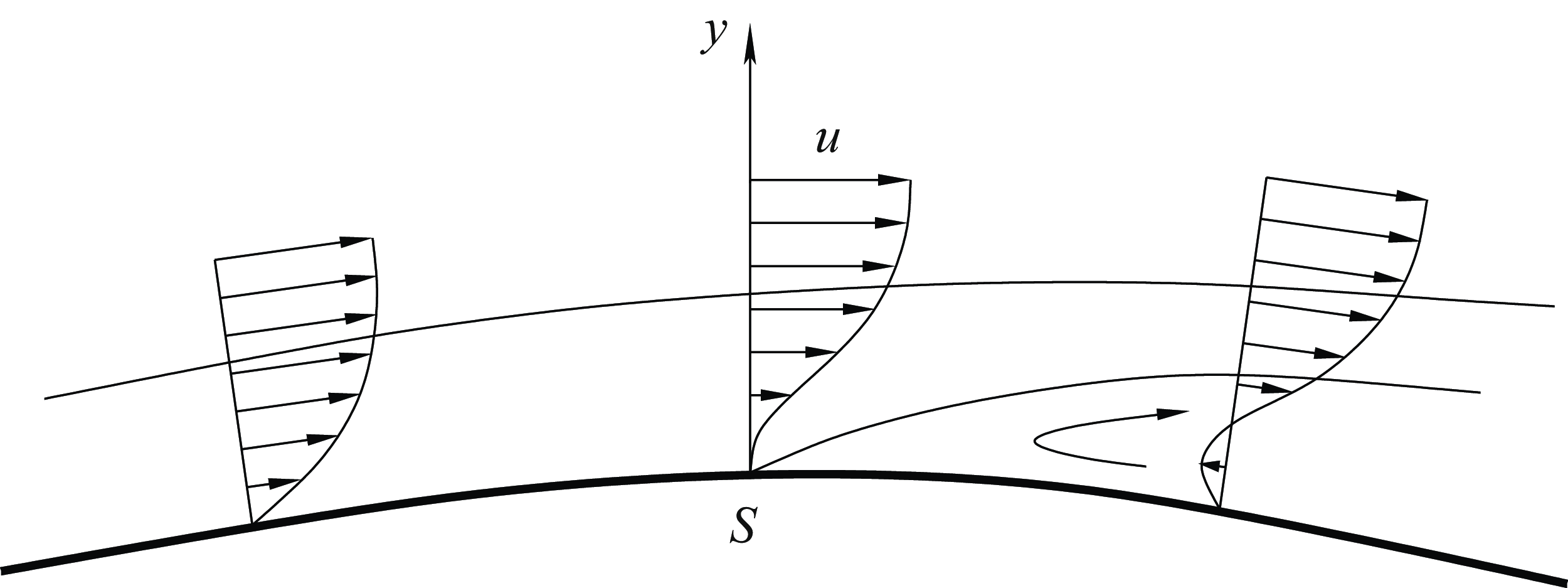
Figure 1. Boundary-layer separation in a steady flow.
The separation point $S$
may be identified as a point on the body contour where the skin friction becomes zero:
$S$
may be identified as a point on the body contour where the skin friction becomes zero:
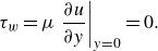 \begin{equation} \tau _w = \mu \left. \frac {\partial u}{\partial y} \right |_{y = 0} = 0 . \end{equation}
Here, we denote the longitudinal velocity by $u$
, the distance from the body surface by
$u$
, the distance from the body surface by $y$
and
$y$
and $\mu$
is the viscosity coefficient. Indeed, with
$\mu$
is the viscosity coefficient. Indeed, with $\tau _w$
being positive upstream of the separation point, the longitudinal velocity
$\tau _w$
being positive upstream of the separation point, the longitudinal velocity $u$
stays positive, which means that the fluid particles in the boundary layer move downstream along the wall and the flow appears to be attached to the body surface. However, once the skin friction turns negative, a layer of reversed flow (
$u$
stays positive, which means that the fluid particles in the boundary layer move downstream along the wall and the flow appears to be attached to the body surface. However, once the skin friction turns negative, a layer of reversed flow ( $u \lt 0$
) forms near the wall, giving rise to a recirculation region.
$u \lt 0$
) forms near the wall, giving rise to a recirculation region.
The situation with unsteady flow separation is more complex. The fact is that the unsteady separation may assume different forms depending on the flow considered. A classical example is the flow past a circular cylinder with the Kármán vortex street in its wake. In this flow, each individual vortex forms near the cylinder surface through accumulation of vorticity in the boundary layer. Once the circulation around the vortex reaches a critical value, it is shed downstream and another one starts to form in its place. During this cycle, the separation point moves up and down the cylinder surface. An important observation concerning this type of flows was made by Sears (Reference Sears1956) and Moore (Reference Moore and Görtler1958). They noticed that the flow near the separation may be treated as quasi-steady, namely, it is described by the steady equations of motion if considered in the coordinate frame moving with the separation point. Of course, the fact that the flow near the separation point is governed by the steady equations does not mean that the theory of steady separation becomes applicable. Indeed, in the frame moving with the separation point, the body surface no longer remains motionless. Figure 2 shows what happens when the separation point moves upstream along the cylinder surface and, correspondingly, for an ‘observer’ in the moving frame, the cylinder surface moves downstream. Due to the action of viscous forces, the fluid particles adjacent to the wall will be involved in the downstream motion, which precludes the recirculation region to start from a point on the body surface, as it happens in the case of steady flow separation. Instead, the separation now takes place from a point that lies in the middle of the boundary layer, as was first suggested by Rott (Reference Rott1956), Sears (Reference Sears1956) and Moore (Reference Moore and Görtler1958). To explain how it happens, let us consider a sequence of cross-sections of the boundary layer corresponding to progressively larger values of the longitudinal coordinate $x$
. In each cross-section, the fluid velocity
$x$
. In each cross-section, the fluid velocity $u$
is a function of the normal coordinate
$u$
is a function of the normal coordinate $y$
. If the boundary layer is exposed to an adverse pressure gradient, then the fluid will experience a deceleration. As a result, the velocity profile will have a minimum that lies some distance
$y$
. If the boundary layer is exposed to an adverse pressure gradient, then the fluid will experience a deceleration. As a result, the velocity profile will have a minimum that lies some distance $y_{min } (x)$
from the wall. If the pressure gradient is strong enough, then the minimal velocity will continue to decrease with
$y_{min } (x)$
from the wall. If the pressure gradient is strong enough, then the minimal velocity will continue to decrease with $x$
, leading to the separation point
$x$
, leading to the separation point $ ( x_s, y_{min } (x_s) )$
, where
$ ( x_s, y_{min } (x_s) )$
, where $u$
is zero. At this point, the so-called Moore–Rott–Sears condition holds.
$u$
is zero. At this point, the so-called Moore–Rott–Sears condition holds.
 \begin{equation} u = \frac {\partial u}{\partial y} = 0 \end{equation}
Behind this point, two recirculation regions form in the boundary layer.

Figure 2. Boundary-layer separation on downstream moving wall.
In both situations depicted in figures 1 and 2, the point of separation may be identified with the onset of the flow reversal in the boundary layer. The case of an upstream moving wall is more difficult, as due to the no-slip requirement, the fluid adjacent to the wall is involved in upstream motion even before separation. Our objective in the present paper is to clarify the topology of the boundary layer separating on the upstream moving wall. We shall use as an example the flow near the leading edge of an aerofoil. The problem is formulated in § 2 based on the classical Prandtl boundary-layer theory. In § 3, we describe the numerical technique that solves the boundary-layer equations. The results of the calculations are presented in § 4. We found that there exists a critical value of the angle of attack. Before it is reached, the solution proves to be regular, which tells us that the boundary layer remains attached to the aerofoil surface. However, at the critical value of the angle of attack, a Moore–Rott–Sears singularity develops (most notably) in the reverse flow region. This is accompanied by an abrupt thickening of the boundary layer at the singular point and the formation of a recirculation region with closed streamlines behind this point. We further find that the flow immediately behind the singular point and in the recirculation region could be treated as inviscid. Using this observation, we offer in § 5 a rather simple theoretical description of the flow. Finally, in the Appendix, we show how the exact solution of Hiemenz (Reference Hiemenz1911) for the front stagnation point may be extended for the flow on a moving wall.
A similar flow was earlier studied by Bezrodnykh, Zametaev & Chzhun (Reference Bezrodnykh, Zametaev and Chzhun2023). These authors considered the boundary layer on a flat plate with the pressure gradient created by a dipole situated some distance from the plate. They found that there exists a critical value of the dipole strength for which a singularity forms in the boundary layer. It was identified as a Moore–Rott–Sears singularity. However, the flow behaviour near the singular point appeared to be rather different from what we see in our calculations.
2. Problem formulation
We shall consider an incompressible fluid flow near the leading edge of a thin aerofoil. To analyse this flow, we shall use Cartesian coordinates $(X^{\prime }, Y^{\prime })$
with the origin situated at the leading edge and the
$(X^{\prime }, Y^{\prime })$
with the origin situated at the leading edge and the $X^{\prime }$
-axis drawn parallel to the middle line of the aerofoil. We shall assume that in the leading-edge region, the aerofoil contour may be represented by the infinite parabola
$X^{\prime }$
-axis drawn parallel to the middle line of the aerofoil. We shall assume that in the leading-edge region, the aerofoil contour may be represented by the infinite parabola $Y^{\prime } = \pm \sqrt {2 X^{\prime }}$
; see figure 3.
$Y^{\prime } = \pm \sqrt {2 X^{\prime }}$
; see figure 3.
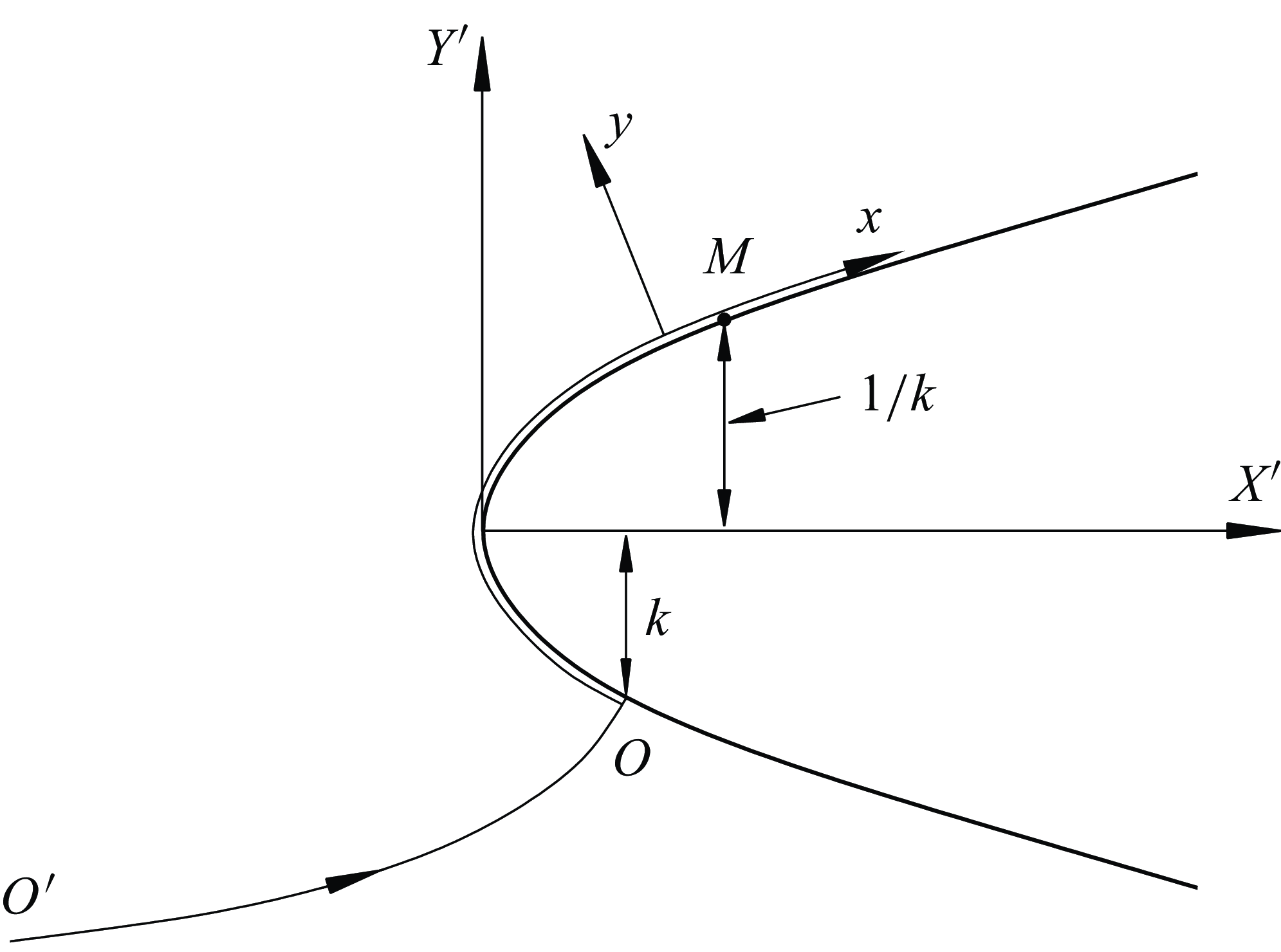
Figure 3. Flow near the leading edge of a thin aerofoil. Here, we use two coordinate systems: Cartesian coordinates $(X^{\prime }, Y^{\prime })$
and body-fitted coordinates
$(X^{\prime }, Y^{\prime })$
and body-fitted coordinates $(x, y)$
. The position of the front stagnation point
$(x, y)$
. The position of the front stagnation point $O$
is given by
$O$
is given by $Y^{\prime } = - k$
, where
$Y^{\prime } = - k$
, where $k$
is the angle of attack parameter.
$k$
is the angle of attack parameter.
2.1. Inviscid flow
The solution of the Euler equations for the inviscid flow past the parabola allows us to find that the tangential velocity on the surface of the parabola is given by
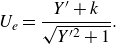 \begin{equation} U_e = \frac {Y^{\prime } + k}{\sqrt {Y^{\prime 2} + 1}} . \end{equation}
Here, $Y^{\prime }$
has to be thought of as the distance from the point on the surface of the parabola, where
$Y^{\prime }$
has to be thought of as the distance from the point on the surface of the parabola, where $U_e$
is to be found, to the axis of symmetry of the parabola. Parameter
$U_e$
is to be found, to the axis of symmetry of the parabola. Parameter $k$
represents the degree of non-symmetry of the flow and may be called the angle of attack parameter. Notice that the stagnation point
$k$
represents the degree of non-symmetry of the flow and may be called the angle of attack parameter. Notice that the stagnation point $O$
, where
$O$
, where $U_e = 0$
, is the point with
$U_e = 0$
, is the point with $Y^{\prime } = - k$
; see figure 3. By differentiating (2.1) with respect to
$Y^{\prime } = - k$
; see figure 3. By differentiating (2.1) with respect to $Y^{\prime }$
and setting the derivative to zero, we can find that the maximum of
$Y^{\prime }$
and setting the derivative to zero, we can find that the maximum of $U_e$
is achieved at point
$U_e$
is achieved at point $M$
, where
$M$
, where $Y^{\prime } = 1/k$
. At this point,
$Y^{\prime } = 1/k$
. At this point,
 \begin{align} U_e \Big|_M = \sqrt {1 + k^2} . \end{align}
Downstream of point $M$
, the tangential velocity
$M$
, the tangential velocity $U_e (x)$
shows monotonic decay and tends to unity as
$U_e (x)$
shows monotonic decay and tends to unity as $x \to \infty$
.
$x \to \infty$
.
For further use, we need to know $U_e$
as a function of the distance
$U_e$
as a function of the distance $x$
measured along the parabola contour from the stagnation point
$x$
measured along the parabola contour from the stagnation point $O$
. We notice that
$O$
. We notice that
 \begin{align} {\rm d} x = \sqrt {({\rm d} X^{\prime })^2 + ({\rm d} Y^{\prime })^2} = {\rm d} Y^{\prime } \sqrt { \left ( \frac {{\rm d} X^{\prime }}{{\rm d} Y^{\prime }} \right ) ^2 + 1} . \end{align}
This means that the sought function $Y^{\prime } (x)$
may be found by solving the differential equation
$Y^{\prime } (x)$
may be found by solving the differential equation
 \begin{equation} \frac {{\rm d} Y^{\prime }}{{\rm d} x} = \frac {1}{\sqrt {1 + Y^{\prime 2}}} \end{equation}
with the initial condition
 \begin{equation} Y^{\prime } = - k \quad \text{at} \quad x = 0 . \end{equation}
This is done numerically. With known solution to (2.4), the velocity at the outer edge of the boundary layer is obtained with the help of (2.1).
2.2. Boundary layer
Our task is to solve the classical boundary-layer equations
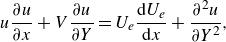 \begin{align} u \frac {\partial u}{\partial x} + V \frac {\partial u}{\partial Y} & = U_e \frac {{\rm d} U_e}{{\rm d} x} + \frac {\partial ^2 u}{\partial Y^2}, \end{align}
 \begin{align} \frac {\partial u}{\partial x} + \frac {\partial V}{\partial Y} & = 0 . \end{align}
We shall impose the usual boundary conditions at the outer edge of the boundary layer and on the body surface:
 \begin{align} u & = U_e (x) \qquad\text{at} \qquad Y = \infty, \end{align}
 \begin{align} u & = U_w, \quad V = 0 \quad \text{at} \quad Y = 0 . \end{align}
In this study, we assume that $U_w$
is negative.
$U_w$
is negative.
In addition to (2.6), (2.5) requires the boundary conditions that specify the behaviour of $u$
as
$u$
as $x \to \infty$
and
$x \to \infty$
and $x \to -\infty$
. The first of these corresponds to the upper surface of the aerofoil and the second to the lower. When formulating these conditions, it is convenient to introduce the stream function
$x \to -\infty$
. The first of these corresponds to the upper surface of the aerofoil and the second to the lower. When formulating these conditions, it is convenient to introduce the stream function $\Psi (x, Y)$
such that
$\Psi (x, Y)$
such that
 \begin{equation} \frac {\partial \Psi }{\partial x} = - V, \qquad \frac {\partial \Psi } {\partial Y} = u . \end{equation}
It follows from (2.1) that
 \begin{align} U_e \to 1 \quad \text{as} \quad x \to \infty . \end{align}
Keeping this in mind, we seek the solution to (2.5) in the form
 \begin{equation} \Psi = \sqrt {x} f (\eta ) + \cdots \quad \text{as} \quad x \to \infty, \end{equation}
where
 \begin{align} \eta = \frac {Y}{\sqrt {x}} . \end{align}
Substitution of (2.9) into (2.7) yields
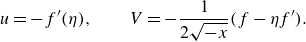
 \begin{equation} u = f^{\prime } (\eta ), \qquad V = - \frac {1}{2 \sqrt {x}} (f - \eta f^{\prime }) . \end{equation}
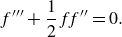
If we now substitute (2.11) into (2.5a
), then we will have the Blasius equation for $f (\eta )$
:
$f (\eta )$
:
 \begin{equation} f^{\prime \prime \prime } + \frac {1}{2} f f^{\prime \prime } = 0 . \end{equation}
The boundary conditions for (2.12) are
 \begin{equation} f (0) = 0, \quad f^{\prime } (0) = U_w, \quad f^{\prime } (\infty ) = 1 . \end{equation}
The boundary-value problem (2.12), (2.13) can be solved numerically for different values of the wall velocity $U_w$
. As an example, in figure 4, we show the velocity profile
$U_w$
. As an example, in figure 4, we show the velocity profile $f^{\prime } (\eta )$
for
$f^{\prime } (\eta )$
for $U_w = -0.1$
. Interestingly enough, we found that the solution of (2.12), (2.13) only exists for
$U_w = -0.1$
. Interestingly enough, we found that the solution of (2.12), (2.13) only exists for $U_w \gt - 0.354$
and shows a ‘hysteresis behaviour’ displayed in figure 5.
$U_w \gt - 0.354$
and shows a ‘hysteresis behaviour’ displayed in figure 5.
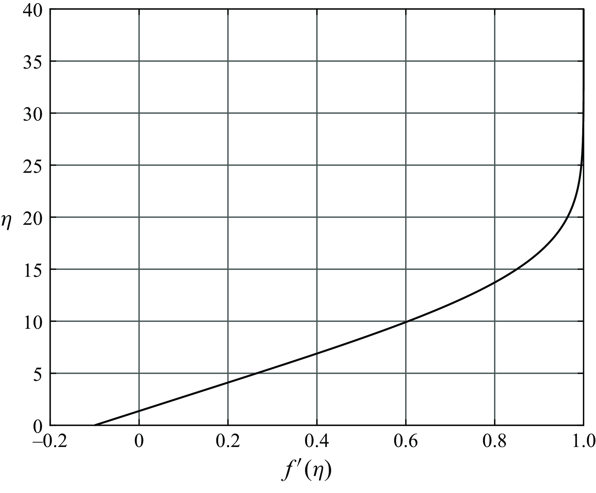
Figure 4. Velocity profile for the Blasius flow on a moving wall with $U_w = -0.1$
.
$U_w = -0.1$
.
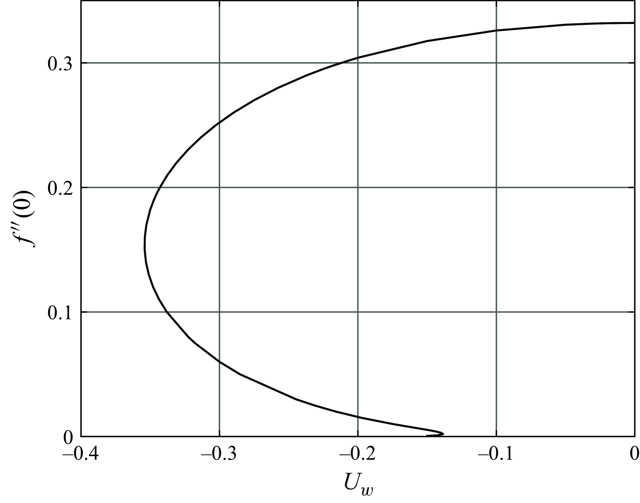
Figure 5. Skin friction $f^{\prime \prime } (0)$
as a function of the wall speed
$f^{\prime \prime } (0)$
as a function of the wall speed $U_w$
.
$U_w$
.
The boundary condition for the lower surface of the aerofoil is formulated in the same way. It follows from (2.1) that
 \begin{align} U_e \to - 1 \quad \text{as} \quad x \to - \infty . \end{align}
Keeping this in mind, we seek the solution to (2.5) in the form
 \begin{equation} \Psi = - \sqrt {- x} f (\eta ) + \cdots \quad \text{as} \quad x \to \infty, \end{equation}
where
 \begin{align} \eta = \frac {Y}{\sqrt {-x}} . \end{align}
Substitution of (2.15) into (2.7) yields
 \begin{equation} u = - f^{\prime } (\eta ), \qquad V = - \frac {1}{2 \sqrt {-x}} (f - \eta f^{\prime }) . \end{equation}
If we now substitute (2.17) into (2.5a
), we will see that $f (\eta )$
satisfies the Blasius equation:
$f (\eta )$
satisfies the Blasius equation:
 \begin{equation} f^{\prime \prime \prime } + \frac {1}{2} f f^{\prime \prime } = 0 . \end{equation}
The boundary conditions for (2.18) are
 \begin{equation} f (0) = 0, \quad f^{\prime } (0) = - U_w, \quad f^{\prime } (\infty ) = 1 . \end{equation}
We found that the solution to (2.18), (2.19) exists for all negative values of $U_w$
.
$U_w$
.
3. Computation technique
The numerical solution of the boundary-layer equations (2.5) was performed in the rectangular computational domain
 \begin{align} x \in [-x_{max }, x_{max }], \quad Y \in [0, Y_{max }], \end{align}
using the uniform mesh
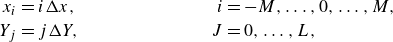 \begin{align} x_i &= i \Delta x, & \quad i &= -M, \ldots, 0, \ldots, M, \nonumber \\ Y_j &= j \Delta Y, & J &= 0, \ldots, L, \end{align}
where $\Delta x$
and
$\Delta x$
and $\Delta Y$
are the mesh steps in the longitudinal and transverse directions. In the internal points of the domain, namely, for
$\Delta Y$
are the mesh steps in the longitudinal and transverse directions. In the internal points of the domain, namely, for $i = -M+1, \ldots, M-1$
,
$i = -M+1, \ldots, M-1$
, $j = 1, \ldots, L-1$
, the derivatives in (2.5) are approximated as
$j = 1, \ldots, L-1$
, the derivatives in (2.5) are approximated as
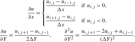 \begin{gather} \frac {\partial u}{\partial x} = \begin{cases} \dfrac {u_{i,j} - u_{i-1,j}}{\Delta x} & \text{if} \;\; u_{i,j} \gt 0, \\[4mm] \dfrac {u_{i+1,j} - u_{i,j}}{\Delta x} & \text{if} \;\; u_{i,j} \lt 0, \end{cases} \nonumber \\ \frac {\partial u}{\partial Y} = \frac {u_{i,j+1} - u_{i,j-1}}{2 \Delta Y}, \qquad \frac {\partial ^2 u}{\partial Y^2} = \frac {u_{i,j+1} - 2 u_{i,j} + u_{i,j-1}} {(\Delta Y)^2} . \end{gather}
This results in the following set of algebraic equations for $u_{i,j}$
on the mesh line
$u_{i,j}$
on the mesh line $x = x_i$
:
$x = x_i$
:
 \begin{equation} a_j \tau _{i,j+1} + b_j \tau _{i,j} + c_j \tau _{i,j-1} = d_j, \qquad j = 1, \ldots, L-1, \end{equation}
with
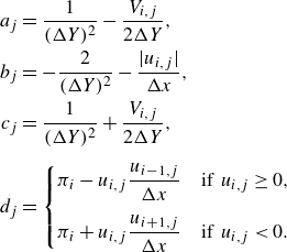 \begin{align} a_j &= \frac {1}{(\Delta Y)^2} - \frac {V_{i,j}}{2 \Delta Y}, \nonumber \\ b_j &= - \frac {2}{(\Delta Y)^2} - \frac {|u_{i,j}|}{\Delta x}, \nonumber \\ c_j &= \frac {1}{(\Delta Y)^2} + \frac {V_{i,j}}{2 \Delta Y}, \nonumber \\[2mm] d_j &= \begin{cases} \pi _i - u_{i,j} \dfrac {u_{i-1,j}}{\Delta x} & \text{if} \;\; u_{i,j} \ge 0, \\[4mm] \pi _i + u_{i,j} \dfrac {u_{i+1,j}}{\Delta x} & \text{if} \;\; u_{i,j} \lt 0 . \end{cases} \end{align}
Here, $\pi _i$
is the negative pressure gradient
$\pi _i$
is the negative pressure gradient $-{\rm d}p/{\rm d}x = U_e {\rm d}U_e/{\rm d}x$
at point
$-{\rm d}p/{\rm d}x = U_e {\rm d}U_e/{\rm d}x$
at point $x_i$
.
$x_i$
.
The set of (3.4) is solved using the Thomas technique. We write
 \begin{equation} u_{i,j} = R_j u_{i,j-1} + Q_j, \qquad j = 1, \ldots, L . \end{equation}
The Thomas coefficients, $R_j$
,
$R_j$
, $Q_j$
are calculated using the recurrent equations
$Q_j$
are calculated using the recurrent equations
 \begin{align} R_j = - \frac {c_j}{b_j + a_j R_{j+1}}, \qquad Q_j = \frac {{\rm d}_j - a_j Q_{j+1}} {b_j + a_j R_{j+1}} \qquad j= L-1, \ldots, 1 . \end{align}
To satisfy the condition $u_{i,L} = U_e (x_i)$
, we set
$u_{i,L} = U_e (x_i)$
, we set
 \begin{align} R_L = 0, \qquad Q_L = U_e (x_i) . \end{align}
Then, (3.6) is used to update the longitudinal velocity $u_{i,j}$
on the mesh line
$u_{i,j}$
on the mesh line $x_i$
. To satisfy the no-slip condition, we set
$x_i$
. To satisfy the no-slip condition, we set $u_{i,0} = U_w$
. An improved approximation to the transverse velocity
$u_{i,0} = U_w$
. An improved approximation to the transverse velocity $V_{i,j}$
is then obtained with the help of the continuity equation (2.5b
). This procedure is repeated for all mesh lines
$V_{i,j}$
is then obtained with the help of the continuity equation (2.5b
). This procedure is repeated for all mesh lines $x_i$
sweeping the computational domain as many times as it requires to achieve the convergence of the iteration process, which is facilitated by making use of an under-relaxation.
$x_i$
sweeping the computational domain as many times as it requires to achieve the convergence of the iteration process, which is facilitated by making use of an under-relaxation.
4. Computational results
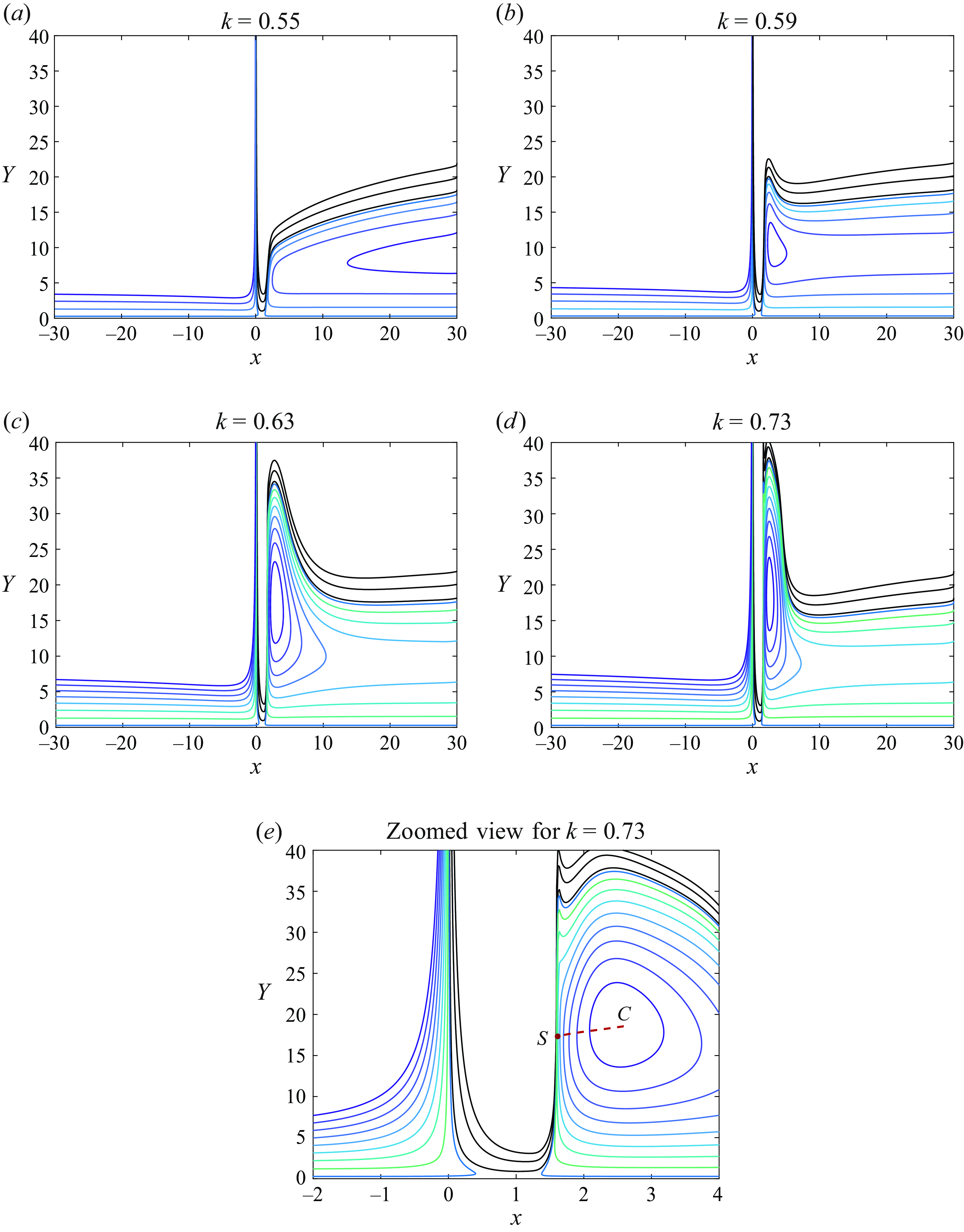
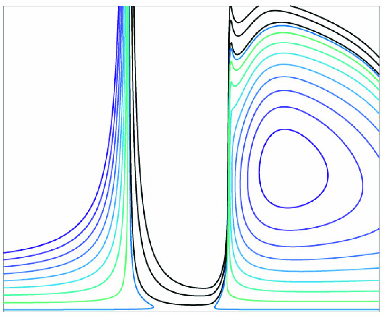
Figure 6. Streamline pattern for the flow in the boundary layer for different values of the angle of attack parameter $k$
.
$k$
.
When performing the calculations, we chose the wall speed to be $U_w = - 0.35$
, which is smaller (by absolute value) than the critical velocity
$U_w = - 0.35$
, which is smaller (by absolute value) than the critical velocity $U_w = -0.354$
. To enhance the convergence of the iteration process, we started with symmetric flow (
$U_w = -0.354$
. To enhance the convergence of the iteration process, we started with symmetric flow ( $k = 0$
) past the parabola (see figure 3) and then the angle of attack parameter
$k = 0$
) past the parabola (see figure 3) and then the angle of attack parameter $k$
was increased step-by-step with the results for the previous value of
$k$
was increased step-by-step with the results for the previous value of $k$
used as an initial guess for a new
$k$
used as an initial guess for a new $k$
. The behaviour of the flow is illustrated in figure 6, where we show how the streamline pattern changes with increasing
$k$
. The behaviour of the flow is illustrated in figure 6, where we show how the streamline pattern changes with increasing $k$
. Remember that we are using the body-fitted coordinates with
$k$
. Remember that we are using the body-fitted coordinates with $x$
measured along the aerofoil surface and
$x$
measured along the aerofoil surface and $Y$
in the perpendicular direction. The streamline
$Y$
in the perpendicular direction. The streamline $O^{\prime } O$
that passes through the front stagnation point
$O^{\prime } O$
that passes through the front stagnation point $O$
(see figure 3) appears to be vertical in figure 6 and, together with the neighbouring streamlines, forms a characteristic ‘spike’ near
$O$
(see figure 3) appears to be vertical in figure 6 and, together with the neighbouring streamlines, forms a characteristic ‘spike’ near $x = 0$
. The region to the right of this ‘spike’ represents the flow on the upper surface of the aerofoil, while the region on the left-hand side corresponds to the flow on the lower surface.
$x = 0$
. The region to the right of this ‘spike’ represents the flow on the upper surface of the aerofoil, while the region on the left-hand side corresponds to the flow on the lower surface.
We found that the boundary layer on the lower side of the aerofoils stays free of singularities, and hence, remains well attached to the aerofoil surface. The behaviour of the boundary layer on the upper surface depends on the angle of attack parameter $k$
. Up to
$k$
. Up to $k = 0.55$
, the streamline pattern does not change much and has an open reverse flow region, as shown in figure 6(a). However, then a bulge starts to grow on the ‘nose’ of this region. Its size increases rather fast as
$k = 0.55$
, the streamline pattern does not change much and has an open reverse flow region, as shown in figure 6(a). However, then a bulge starts to grow on the ‘nose’ of this region. Its size increases rather fast as $k$
becomes larger. This is accompanied by the formation of a recirculation region with closed streamlines; see figure 6(b–d).
$k$
becomes larger. This is accompanied by the formation of a recirculation region with closed streamlines; see figure 6(b–d).
The results of the calculations further suggest that there exists a critical value $k_c$
of parameter
$k_c$
of parameter $k$
, slightly larger than
$k$
, slightly larger than $k = 0.73$
, for which the solution develops a singularity. The singular point
$k = 0.73$
, for which the solution develops a singularity. The singular point $S$
lies on the line of zero longitudinal velocity
$S$
lies on the line of zero longitudinal velocity $u$
, which is shown in figure 6(e) as a dashed line
$u$
, which is shown in figure 6(e) as a dashed line $S C$
; in what follows, we shall call it the ‘Zero-
$S C$
; in what follows, we shall call it the ‘Zero- $u$
-Line’, and define its position as
$u$
-Line’, and define its position as $Y = Z (x)$
. The singularity manifests itself by convergence of the streamlines at point
$Y = Z (x)$
. The singularity manifests itself by convergence of the streamlines at point $S$
as
$S$
as $k \to k_c$
. The formation of the singularity is illustrated in figure 7, where we show the distribution of the shear stress
$k \to k_c$
. The formation of the singularity is illustrated in figure 7, where we show the distribution of the shear stress $\partial u / \partial Y$
along the Zero-
$\partial u / \partial Y$
along the Zero- $u$
-Line for
$u$
-Line for $k \lt k_c$
. Notice that the corresponding graphs are extended into a region before the singular point whose coordinate is
$k \lt k_c$
. Notice that the corresponding graphs are extended into a region before the singular point whose coordinate is $x_s \approx 1.6$
. We see that
$x_s \approx 1.6$
. We see that $\partial u / \partial Y$
develops a characteristic minimum, the value of which becomes smaller as
$\partial u / \partial Y$
develops a characteristic minimum, the value of which becomes smaller as $k$
increases, and finally becomes zero at
$k$
increases, and finally becomes zero at $k = k_c$
. This confirms that the singular point
$k = k_c$
. This confirms that the singular point $S$
is in fact a Moore–Rott–Sears point; see conditions (1.2). Interestingly enough, at this point, the pressure gradient is favourable (
$S$
is in fact a Moore–Rott–Sears point; see conditions (1.2). Interestingly enough, at this point, the pressure gradient is favourable ( ${\rm d}p/{\rm d}x \lt 0$
) as first predicted by Ruban et al. (Reference Ruban, Djehizian, Kirsten and Kravtsova2020) and then confirmed by Bezrodnykh et al. (Reference Bezrodnykh, Zametaev and Chzhun2023).
${\rm d}p/{\rm d}x \lt 0$
) as first predicted by Ruban et al. (Reference Ruban, Djehizian, Kirsten and Kravtsova2020) and then confirmed by Bezrodnykh et al. (Reference Bezrodnykh, Zametaev and Chzhun2023).
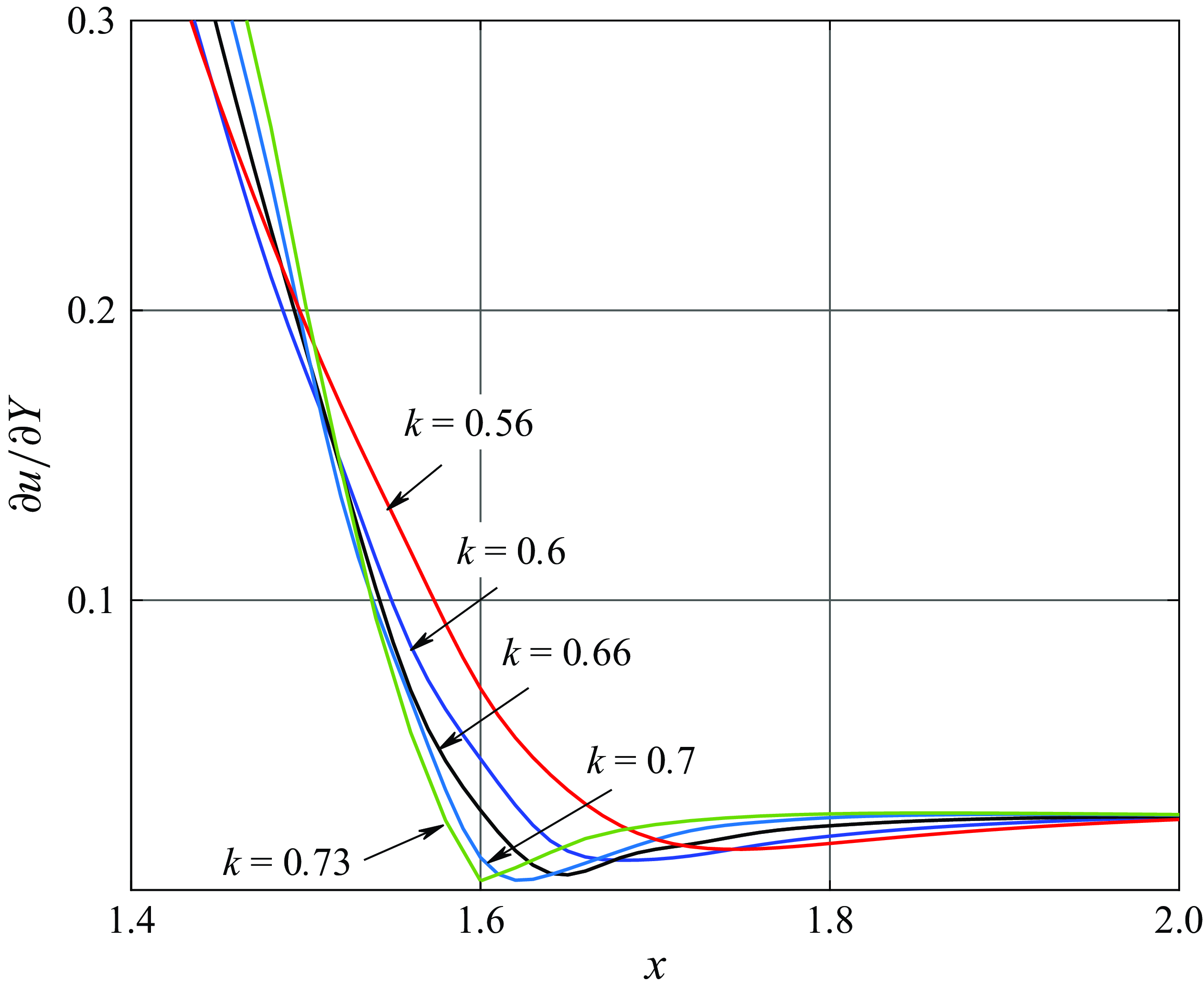
Figure 7. Shear stress distribution along the Zero- $u$
-Line.
$u$
-Line.
The shape of the Zero- $u$
-Line,
$u$
-Line, $Y = Z (x)$
, obtained in the course of our calculations for
$Y = Z (x)$
, obtained in the course of our calculations for $U_w = - 0.35$
and
$U_w = - 0.35$
and $k = 0.73$
, is shown in figure 8(a). In figure 8(b), we show again the shear stress
$k = 0.73$
, is shown in figure 8(a). In figure 8(b), we show again the shear stress $\partial u / \partial Y$
distribution along this line, this time for a larger range of
$\partial u / \partial Y$
distribution along this line, this time for a larger range of $x$
. It is interesting to notice that the shear stress remains almost constant over the recirculation region. This is because, in the boundary-layer approximation,
$x$
. It is interesting to notice that the shear stress remains almost constant over the recirculation region. This is because, in the boundary-layer approximation, $\partial u / \partial Y$
coincides with the vorticity which, according to the Prandtl–Batchelor theorem, should be constant inside a region with closed streamlines (see Batchelor Reference Batchelor1956).
$\partial u / \partial Y$
coincides with the vorticity which, according to the Prandtl–Batchelor theorem, should be constant inside a region with closed streamlines (see Batchelor Reference Batchelor1956).
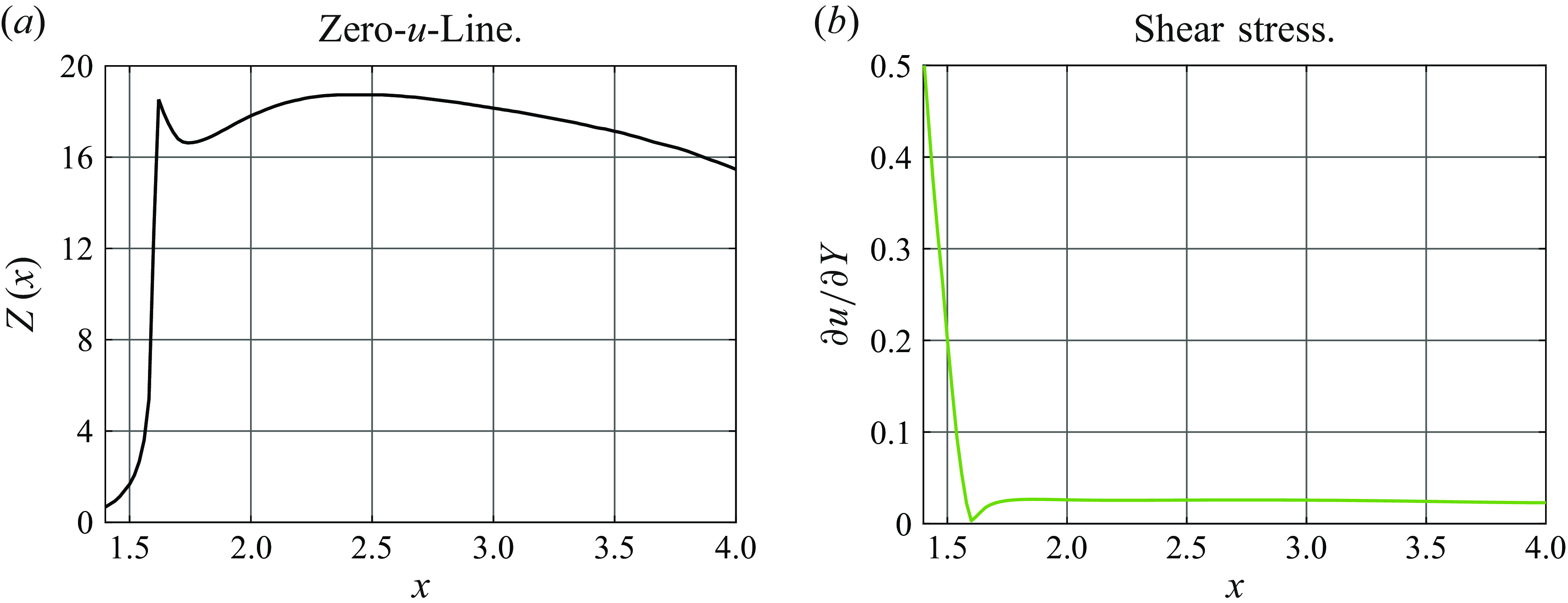
Figure 8. Shape of the Zero- $u$
-Line, and the shear stress distribution along this line for
$u$
-Line, and the shear stress distribution along this line for $U_w = -0.35$
and
$U_w = -0.35$
and $k = 0.73$
.
$k = 0.73$
.
To clarify what happens near point $S$
, where the shear stress becomes zero, we notice that at any point on the Zero-
$S$
, where the shear stress becomes zero, we notice that at any point on the Zero- $u$
-Line
$u$
-Line $S C$
, the momentum equation (2.5a
) reduces to
$S C$
, the momentum equation (2.5a
) reduces to
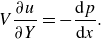 \begin{equation} V \frac {\partial u}{\partial Y} = - \frac {{\rm d} p}{{\rm d} x} . \end{equation}
Here, it is taken into account that the recirculation region is much thicker than the original boundary layer, which allows us to disregard the viscous term on the right-hand side of (2.5a
). In § 5.2, we shall show that the flow remains inviscid in the vicinity of point $S$
. The observed convergence of the streamlines on approach to point
$S$
. The observed convergence of the streamlines on approach to point $S$
tells us that
$S$
tells us that $V$
becomes infinitely large and it follows from (4.1) that
$V$
becomes infinitely large and it follows from (4.1) that $\partial u / \partial Y$
does indeed tend to zero, which means that point
$\partial u / \partial Y$
does indeed tend to zero, which means that point $S$
cannot be inside the Prandtl–Batchelor recirculation region. Instead, it lies in front of this region.
$S$
cannot be inside the Prandtl–Batchelor recirculation region. Instead, it lies in front of this region.
If we take a point just above the line $S C$
, then we can see from figure 6(e) that the longitudinal velocity
$S C$
, then we can see from figure 6(e) that the longitudinal velocity $u$
is positive. It is, of course, zero on
$u$
is positive. It is, of course, zero on $S C$
and becomes negative below
$S C$
and becomes negative below $S C$
. Therefore,
$S C$
. Therefore, $\partial u / \partial Y$
is positive on the line
$\partial u / \partial Y$
is positive on the line $S C$
. Taking further into account that the vertical velocity
$S C$
. Taking further into account that the vertical velocity $V$
is positive on
$V$
is positive on $S C$
, we can conclude that the left-hand side of (4.1) is positive which is only possible if the pressure gradient is favourable, i.e.
$S C$
, we can conclude that the left-hand side of (4.1) is positive which is only possible if the pressure gradient is favourable, i.e. ${\rm d} p / {\rm d} x \lt 0$
.
${\rm d} p / {\rm d} x \lt 0$
.
Of course, the Zero- $u$
-Line can be extended to the right of the centre
$u$
-Line can be extended to the right of the centre $C$
of the recirculation region; see figure 6(e). On this extension,
$C$
of the recirculation region; see figure 6(e). On this extension, $\partial u / \partial Y$
remains positive, but
$\partial u / \partial Y$
remains positive, but $V$
is now negative, which requires the pressure gradient to be adverse, that is,
$V$
is now negative, which requires the pressure gradient to be adverse, that is, ${\rm d} p / {\rm d} x \gt 0$
. Thus, the centre
${\rm d} p / {\rm d} x \gt 0$
. Thus, the centre $C$
of the recirculation region coincides with the position of the zero pressure gradient.
$C$
of the recirculation region coincides with the position of the zero pressure gradient.
5. Theoretical modelling
A distinctive feature of the flow studied here is the formation of a large recirculation region inside the boundary layer. In this region, the fluid close to the wall moves upstream against growing pressure. It decelerates, turns upwards and then, after reaching the Zero- $u$
-Line, starts to move downstream under the action of a favourable pressure gradient. The fluid velocity in the recirculation region is rather small compared with the velocity at the outer edge of the boundary layer, and the thickness of the recirculation region is large compared with that near the front stagnation point. This recirculation region poses an obstacle for the boundary layer flowing towards it from the front stagnation point. Instead of penetrating the recirculation region, this boundary layer climbs on top of it, adding very little to the displacement thickness of the entire boundary layer. Our goal now will be to describe theoretically the flow in the recirculation region and to find the shape of its outer boundary. We shall first consider the main body of the recirculation region where the Prandtl–Batchelor theorem holds. Then, a close vicinity of the singular point
$u$
-Line, starts to move downstream under the action of a favourable pressure gradient. The fluid velocity in the recirculation region is rather small compared with the velocity at the outer edge of the boundary layer, and the thickness of the recirculation region is large compared with that near the front stagnation point. This recirculation region poses an obstacle for the boundary layer flowing towards it from the front stagnation point. Instead of penetrating the recirculation region, this boundary layer climbs on top of it, adding very little to the displacement thickness of the entire boundary layer. Our goal now will be to describe theoretically the flow in the recirculation region and to find the shape of its outer boundary. We shall first consider the main body of the recirculation region where the Prandtl–Batchelor theorem holds. Then, a close vicinity of the singular point $S$
will be analysed.
$S$
will be analysed.
5.1. Prandtl–Batchelor region
We shall start with the following comment. Strictly speaking, for the Prandtl–Batchelor theorem to be valid, the recirculation region has to be asymptotically large on the boundary-layer scale. Our calculations alone cannot prove this, which means that for now, the analysis in § 5.1 should be interpreted as an ‘approximation’.
Assuming that the flow in this region may be treated as inviscid, we use the Bernoulli equation. In the boundary-layer approximation, it is written as
 \begin{equation} \frac {1}{2} u^2 + p = H (\Psi ) . \end{equation}
Here, $H (\Psi )$
is the Bernoulli function which depends on the stream function
$H (\Psi )$
is the Bernoulli function which depends on the stream function $\Psi$
only. Differentiation of (5.1) with respect to
$\Psi$
only. Differentiation of (5.1) with respect to $Y$
shows that
$Y$
shows that
 \begin{align} u \frac {\partial u}{\partial Y} = \frac {{\rm d} H}{{\rm d} \Psi } \frac {\partial \Psi }{\partial Y} . \end{align}
Since $\partial \Psi / \partial Y = u$
, we can conclude that
$\partial \Psi / \partial Y = u$
, we can conclude that
 \begin{equation} \frac {{\rm d} H}{{\rm d} \Psi } = \frac {\partial u}{\partial Y} = \omega . \end{equation}
Here, $\omega$
is the vorticity. In the region considered, it is constant being equal to approximately
$\omega$
is the vorticity. In the region considered, it is constant being equal to approximately $0.0255$
; see figure 8(b). Integrating (5.3), we have
$0.0255$
; see figure 8(b). Integrating (5.3), we have
 \begin{equation} H = \omega \Psi + \mathcal{C} . \end{equation}
To find constant $\mathcal{C}$
, we consider a point that lies on the Zero-
$\mathcal{C}$
, we consider a point that lies on the Zero- $u$
-Line and assume that this point tends to the singular point
$u$
-Line and assume that this point tends to the singular point $S$
. In this limit,
$S$
. In this limit, $u$
stays zero and
$u$
stays zero and $p$
tends to
$p$
tends to $p_s$
. Therefore, it follows from (5.1) that
$p_s$
. Therefore, it follows from (5.1) that $H (\Psi _s)= p_s$
, where
$H (\Psi _s)= p_s$
, where $\Psi _s$
is the value of the stream function
$\Psi _s$
is the value of the stream function $\Psi$
at point
$\Psi$
at point $S$
. Using (5.4), we can now see that
$S$
. Using (5.4), we can now see that $\mathcal{C} = p_s - \omega \Psi _s$
. Hence, we can conclude that
$\mathcal{C} = p_s - \omega \Psi _s$
. Hence, we can conclude that
 \begin{equation} H = p_s + \omega (\Psi - \Psi _s) . \end{equation}
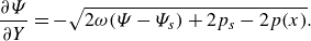
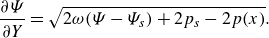
Substituting (5.5) into (5.1) and solving the resulting equation for $u$
, we have
$u$
, we have
 \begin{equation} u = \pm \sqrt {2 \omega (\Psi - \Psi _s) + 2 p_s - 2 p (x)} . \end{equation}
Let us first consider the flow region below the Zero- $u$
-Line. In this region,
$u$
-Line. In this region, $u \lt 0$
, and using the fact that
$u \lt 0$
, and using the fact that $u = \partial \Psi / \partial Y$
, we can write (5.6) as
$u = \partial \Psi / \partial Y$
, we can write (5.6) as
 \begin{equation} \frac {\partial \Psi }{\partial Y} = - \sqrt {2 \omega (\Psi - \Psi _s) + 2 p_s - 2 p (x)} . \end{equation}
Equation (5.7) is easily integrated with respect to $Y$
to yield
$Y$
to yield
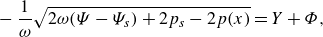 \begin{equation} - \frac {1}{\omega } \sqrt {2 \omega (\Psi - \Psi _s) + 2 p_s - 2 p (x)} = Y + \Phi, \end{equation}
where $\Phi$
is an arbitrary function of
$\Phi$
is an arbitrary function of $x$
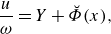
. To find this function, we notice that (5.8) may be written as
$x$
. To find this function, we notice that (5.8) may be written as
 \begin{align} \frac {u}{\omega } = Y + \Phi . \end{align}
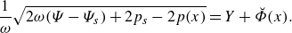
Therefore, if we consider the Zero- $u$
-Line,
$u$
-Line, $Y = Z (x)$
, then we can easily see that
$Y = Z (x)$
, then we can easily see that $\Phi = - Z (x)$
which, being substituted into (5.8), yields
$\Phi = - Z (x)$
which, being substituted into (5.8), yields
 \begin{equation} Y = Z (x) - \frac {1}{\omega } \sqrt {2 \omega (\Psi - \Psi _s) + 2 p_s - 2 p (x)} . \end{equation}
Let us now consider the streamline that passes through the singular point $S$
; see figure 6(e). This streamline represents the boundary between the recirculation and the flow approaching point
$S$
; see figure 6(e). This streamline represents the boundary between the recirculation and the flow approaching point $S$
from the left. We shall call it the ‘dividing streamline’ and define it by the equation
$S$
from the left. We shall call it the ‘dividing streamline’ and define it by the equation $Y = D (x)$
. First, we look at the lower branch of the dividing streamline. After emerging from point
$Y = D (x)$
. First, we look at the lower branch of the dividing streamline. After emerging from point $S$
, it goes down almost vertically, and then turns and extends parallel to the body surface lying at the outer edge of the viscous near-wall layer. Assuming that the thickness of the viscous layer is small compared with the distance from the Zero-
$S$
, it goes down almost vertically, and then turns and extends parallel to the body surface lying at the outer edge of the viscous near-wall layer. Assuming that the thickness of the viscous layer is small compared with the distance from the Zero- $u$
-Line
$u$
-Line $S C$
to the wall, we shall set
$S C$
to the wall, we shall set $Y = 0$
on the left-hand side of (5.10). Keeping further in mind that on the streamline considered,
$Y = 0$
on the left-hand side of (5.10). Keeping further in mind that on the streamline considered, $\Psi = \Psi _s$
, we have
$\Psi = \Psi _s$
, we have
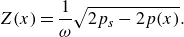 \begin{equation} Z (x) = \frac {1}{\omega } \sqrt {2 p_s - 2 p (x)} . \end{equation}
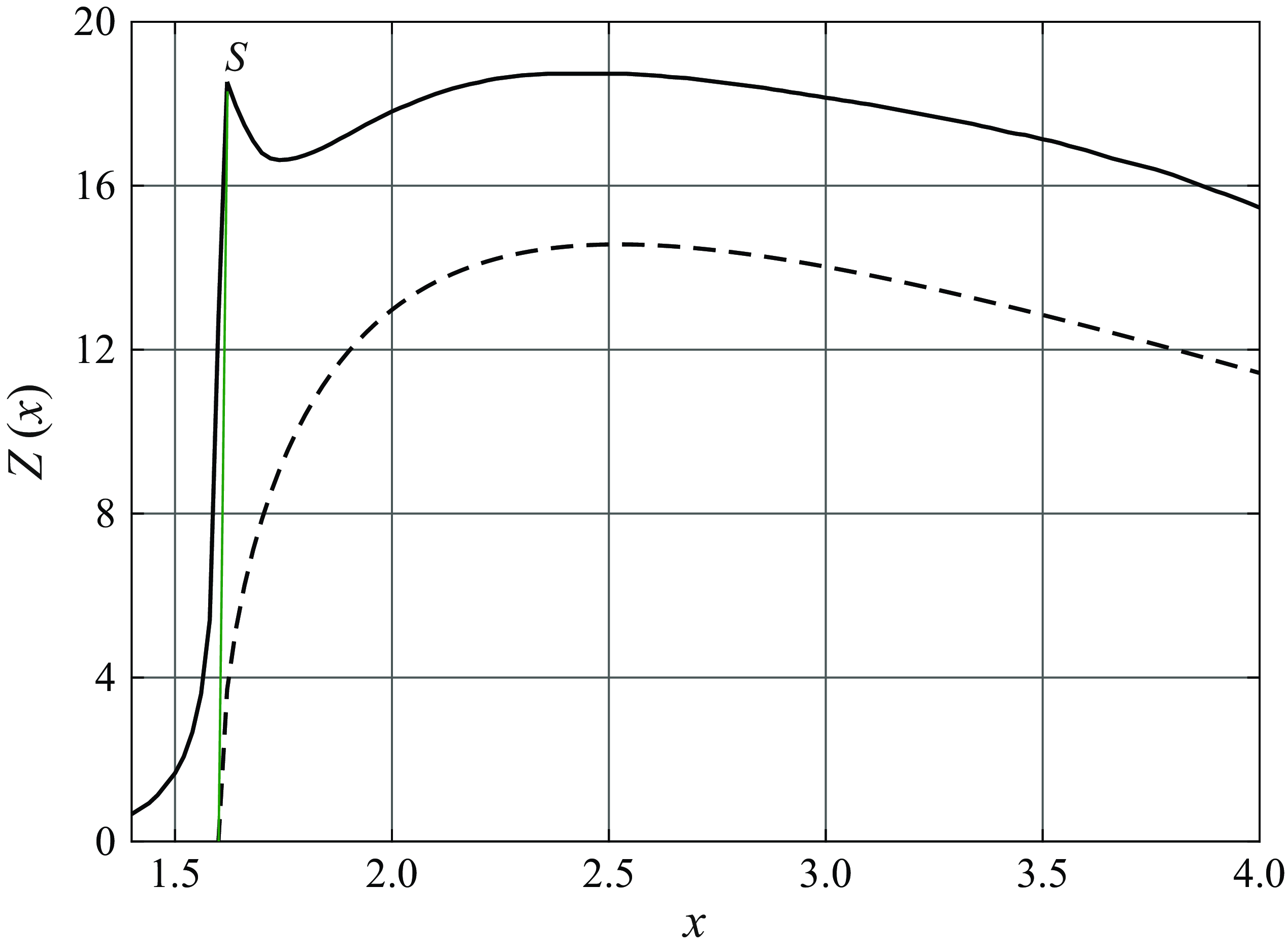
Figure 9. Zero- $u$
-line. Comparison of the numerical results (solid line) with theoretical predictions (dashed line).
$u$
-line. Comparison of the numerical results (solid line) with theoretical predictions (dashed line).
In figure 9, we compare the theoretical predictions (5.11) with numerical results shown earlier in figure 8(a). We see that on the interval $x \in [1.9, 4.0]$
, the theoretical curve reproduces the shape of the numerical curve perfectly well, but lies below it. This situation can be improved if one takes into account the existence of the viscous layer and adds its thickness to the right-hand side of (5.11). No such easy correction is possible in the region
$x \in [1.9, 4.0]$
, the theoretical curve reproduces the shape of the numerical curve perfectly well, but lies below it. This situation can be improved if one takes into account the existence of the viscous layer and adds its thickness to the right-hand side of (5.11). No such easy correction is possible in the region $x \in [1.6, 1.9]$
that lies immediately behind the singular point
$x \in [1.6, 1.9]$
that lies immediately behind the singular point $S$
. The reason is that point
$S$
. The reason is that point $S$
lies outside the Prandtl–Batchelor recirculation region making (5.5) inapplicable. Figure 9 shows that behind point
$S$
lies outside the Prandtl–Batchelor recirculation region making (5.5) inapplicable. Figure 9 shows that behind point $S$
, the Zero-
$S$
, the Zero- $u$
-Line first goes down sharply, then reaches a minimum and only after that starts to repeat the theoretical prediction (5.11). A detailed analysis of the flow in the vicinity of point
$u$
-Line first goes down sharply, then reaches a minimum and only after that starts to repeat the theoretical prediction (5.11). A detailed analysis of the flow in the vicinity of point $S$
will be presented in § 5.2. Before this, we shall continue with the study of the flow in the Prandtl–Batchelor region and apply our theory to the upper half of the recirculation region.
$S$
will be presented in § 5.2. Before this, we shall continue with the study of the flow in the Prandtl–Batchelor region and apply our theory to the upper half of the recirculation region.
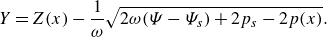
In the flow above the Zero- $u$
-Line, the longitudinal velocity
$u$
-Line, the longitudinal velocity $u$
is positive, and therefore, instead of (5.7), we have to write
$u$
is positive, and therefore, instead of (5.7), we have to write
 \begin{equation} \frac {\partial \Psi }{\partial Y} = \sqrt {2 \omega (\Psi - \Psi _s) + 2 p_s - 2 p (x)} . \end{equation}
Integration of (5.12) yields
 \begin{equation} \frac {1}{\omega } \sqrt {2 \omega (\Psi - \Psi _s) + 2 p_s - 2 p (x)} = Y + \breve {\Phi } (x) . \end{equation}
To find the function $\breve {\Phi } (x)$
, we write (5.13) in the form
$\breve {\Phi } (x)$
, we write (5.13) in the form
 \begin{align} \frac {u}{\omega } = Y + \breve {\Phi } (x), \end{align}
and consider the Zero- $u$
-Line,
$u$
-Line, $Y = Z (x)$
. We see that
$Y = Z (x)$
. We see that $\breve {\Phi } = - Z (x)$
which, being substituted into (5.13), allows us to conclude that
$\breve {\Phi } = - Z (x)$
which, being substituted into (5.13), allows us to conclude that
 \begin{equation} Y = Z (x) + \frac {1}{\omega } \sqrt {2 \omega (\Psi - \Psi _s) + 2 p_s - 2 p (x)} . \end{equation}
The outer boundary of the recirculation region, $Y = D (x)$
, can now be found by setting
$Y = D (x)$
, can now be found by setting $\Psi = \Psi _s$
in (5.15). We have
$\Psi = \Psi _s$
in (5.15). We have
 \begin{align} D (x) = Z (x) + \frac {1}{\omega } \sqrt {2 p_s - 2 p (x)} = \frac {2}{\omega } \sqrt {2 p_s - 2 p (x)} . \end{align}
5.2. Flow immediately behind the singularity
When dealing with the flow in the vicinity of point $S$
, it is convenient to use the coordinate system
$S$
, it is convenient to use the coordinate system $(\breve {x}, \breve {Y})$
with
$(\breve {x}, \breve {Y})$
with $\breve {x}$
measured from point
$\breve {x}$
measured from point $S$
along the Zero-
$S$
along the Zero- $u$
-Line and
$u$
-Line and $\breve {Y}$
in the perpendicular direction. These ‘new’ coordinates are given by
$\breve {Y}$
in the perpendicular direction. These ‘new’ coordinates are given by
 \begin{equation} \breve {x} = x - x_s, \qquad \breve {Y} = Y - Z (x) . \end{equation}
If we define the stream function $\breve {\Psi }$
and the velocity components
$\breve {\Psi }$
and the velocity components $(\breve {U}, \breve {V})$
in the new coordinates via the Prandtl transposition
$(\breve {U}, \breve {V})$
in the new coordinates via the Prandtl transposition
 \begin{align} \breve {\Psi } = \Psi, \quad \;\; \breve {u} = u, \quad \;\; \breve {V} = V - u \frac {{\rm d} Z}{{\rm d} x}, \end{align}
then the boundary layer (2.5) will remain unchanged. We seek the solution to these equations in the form
 \begin{equation} \breve {\Psi } = \Psi _s + \breve {x}^{\alpha } f (\eta ) + \cdots \quad \text{as} \quad \breve {x} \to 0^{+}, \end{equation}
with
 \begin{equation} \eta = \frac {\breve {Y}}{\breve {x}^{\beta }} . \end{equation}
Here, parameters $\alpha$
,
$\alpha$
, $\beta$
and function
$\beta$
and function $f (\eta )$
are to be found in the course of the flow analysis.
$f (\eta )$
are to be found in the course of the flow analysis.
Using (5.19), (5.20), we find that the velocity components
 \begin{align} &\qquad \breve {u} = \frac {\partial \breve {\Psi }}{\partial \breve {Y}} = \breve {x}^{\alpha - \beta } f^{\prime } (\eta ) + \cdots, \end{align}
 \begin{align} & \breve {V} = - \frac {\partial \breve {\Psi }}{\partial \breve {x}} = - \breve {x}^{\alpha - 1} \left [ \alpha f - \beta \eta f^{\prime } \right ] + \cdots . \end{align}
We further find that
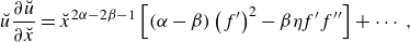 \begin{align} &\breve {u} \frac {\partial \breve {u}}{\partial \breve {x}} = \breve {x}^{2 \alpha - 2 \beta - 1} \left [ (\alpha - \beta ) \left ( f^{\prime } \right ) ^2 - \beta \eta f^{\prime } f^{\prime \prime } \right ] + \cdots, \end{align}
 \begin{align} &\qquad \breve {V} \frac {\partial \breve {u}}{\partial \breve {Y}} = \breve {x}^{2 \alpha - 2 \beta - 1} \left [ - \alpha f f^{\prime \prime } + \beta \eta f^{\prime } f^{\prime \prime } \right ] + \cdots, \end{align}
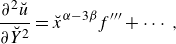 \begin{align} &\qquad\qquad\qquad \frac {\partial ^2 \breve {u}}{\partial \breve {Y}^2} = \breve {x}^{\alpha - 3 \beta } f^{\prime \prime \prime } + \cdots, \end{align}
and since at point $S$
the pressure gradient is favourable, we shall write
$S$
the pressure gradient is favourable, we shall write
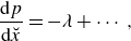 \begin{equation} \frac {{\rm d} p}{{\rm d} \breve {x}} = - \lambda + \cdots, \end{equation}
where $\lambda$
is a known positive constant.
$\lambda$
is a known positive constant.
In the flow considered, the fluid particles accelerate, decelerate and change their direction under the action of the pressure gradient. This means that the pressure gradient (5.22d ) should be the same order quantity as the convective terms (5.22a ), (5.22b ). Consequently, we have to set
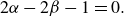 \begin{equation} 2 \alpha - 2 \beta - 1 = 0 . \end{equation}
To evaluate the importance of the viscous forces, we consider the vertical velocity component given by the second equation in (5.21). On the Zero- $u$
-Line, where
$u$
-Line, where $\eta = 0$
, we have
$\eta = 0$
, we have
 \begin{equation} \breve {V} = \breve {x}^{\alpha - 1} \left [ - \alpha f (0) \right ] . \end{equation}
We know that $\breve {V}$
is positive on the Zero-
$\breve {V}$
is positive on the Zero- $u$
-Line, which means that
$u$
-Line, which means that $f (0)$
is negative. Taking logarithms on both sides of (5.24) yields
$f (0)$
is negative. Taking logarithms on both sides of (5.24) yields
 \begin{equation} \ln \breve {V} = (\alpha - 1) \ln \breve {x} + \ln \left [- \alpha f (0) \right ] . \end{equation}
In figure 10, we compare the theoretical prediction (5.25) with the results of the numerical analysis of the flow. The latter is represented by the black curve. The theoretical red curve is a straight line
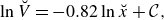 \begin{equation} \ln \breve {V} = - 0.82 \ln \breve {x} + \mathcal{C}, \end{equation}
with $\mathcal{C}$
being a constant. The coefficient
$\mathcal{C}$
being a constant. The coefficient $-0.82$
is chosen to make this line parallel to the black line for small values of
$-0.82$
is chosen to make this line parallel to the black line for small values of $\breve {x}$
. Comparing (5.26) with (5.25), we can see that
$\breve {x}$
. Comparing (5.26) with (5.25), we can see that
 \begin{equation} \alpha \approx \frac {1}{5}, \end{equation}
and then it follows from (5.23) that
 \begin{equation} \beta \approx - \frac {3}{10} . \end{equation}
In § 5.3, the numerical prediction (5.27) for $\alpha$
will be confirmed analytically.
$\alpha$
will be confirmed analytically.

Figure 10. Calculation of the parameter $\alpha$
.
$\alpha$
.
With (5.27) and (5.28), the viscous term (5.22c
) tends to zero as $\breve {x} \to 0^{+}$
, while the convective terms (5.22a
), (5.22b
) and the pressure gradient (5.22d
) remain finite. Hence, we can conclude that the flow considered is predominantly inviscid. Substitution of (5.22) into (2.5a
) results in the following equation for
$\breve {x} \to 0^{+}$
, while the convective terms (5.22a
), (5.22b
) and the pressure gradient (5.22d
) remain finite. Hence, we can conclude that the flow considered is predominantly inviscid. Substitution of (5.22) into (2.5a
) results in the following equation for $f (\eta )$
:
$f (\eta )$
:
 \begin{equation} \frac {1}{2} f^{\prime 2} - \alpha f f^{\prime \prime } = \lambda . \end{equation}
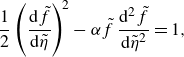
This equation should be solved with the initial conditions
 \begin{equation} \left . \begin{aligned} f &= f (0), \\ f^{\prime } &= 0, \end{aligned} \right \} \quad \text{at} \quad \eta = 0 . \end{equation}
Remember that $f (0)$
in the first condition is negative. The second condition is deduced using the first equation in (5.21) and the fact that the longitudinal velocity
$f (0)$
in the first condition is negative. The second condition is deduced using the first equation in (5.21) and the fact that the longitudinal velocity $u$
is zero on Zero-
$u$
is zero on Zero- $u$
-Line,
$u$
-Line, $S C$
; see figure 6(e).
$S C$
; see figure 6(e).
The affine transformations
 \begin{equation} f = | f (0) | \tilde {f}, \qquad \eta = \frac {| f (0) |}{\sqrt {\lambda }} \tilde {\eta } \end{equation}
 \begin{gather} \frac {1}{2} \left ( \frac {{\rm d} \tilde {f}}{{\rm d} \tilde {\eta }} \right ) ^{\! 2} - \alpha \tilde {f} \,\frac {{\rm d}^2 \tilde {f}}{{\rm d} \tilde {\eta }^2} = 1, \end{gather}
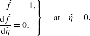 \begin{gather} \left . \begin{aligned} \tilde {f} &= - 1, \\ \frac {{\rm d} \tilde {f}}{{\rm d} \tilde {\eta }} &= 0, \end{aligned} \right \} \quad \text{at} \quad \tilde {\eta } = 0 . \end{gather}
Using the substitution
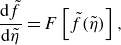 \begin{equation} \frac {{\rm d} \tilde {f}}{{\rm d} \tilde {\eta }} = F \left [ \tilde {f} (\tilde {\eta }) \right ], \end{equation}
we reduce (5.32) to the first-order differential equation
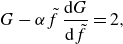 \begin{equation} G - \alpha \tilde {f} \,\frac {{\rm d} G}{{\rm d} \tilde {f}} = 2, \end{equation}
where $G = F^2$
.
$G = F^2$
.
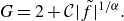
The general solution of (5.35) is written as
 \begin{align} G = 2 + \mathcal{C} |\tilde {f}|^{1/\alpha } . \end{align}
To find constant $\mathcal{C}$
, we use the boundary conditions (5.33), from which it follows that
$\mathcal{C}$
, we use the boundary conditions (5.33), from which it follows that
 \begin{align} G = 0 \quad \text{at} \quad \tilde {f} = - 1 . \end{align}
We see that $\mathcal{C} = - 2$
. Hence,
$\mathcal{C} = - 2$
. Hence,
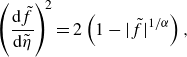 \begin{align} \left ( \frac {{\rm d} \tilde {f}}{{\rm d} \tilde {\eta }} \right ) ^{\! 2} = 2 \left ( 1 - |\tilde {f}|^{1/\alpha } \right ), \end{align}
and we can conclude that
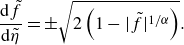 \begin{equation} \frac {{\rm d} \tilde {f}}{{\rm d} \tilde {\eta }} = \pm \sqrt {2 \left ( 1 - |\tilde {f}|^{1/\alpha } \right ) } . \end{equation}
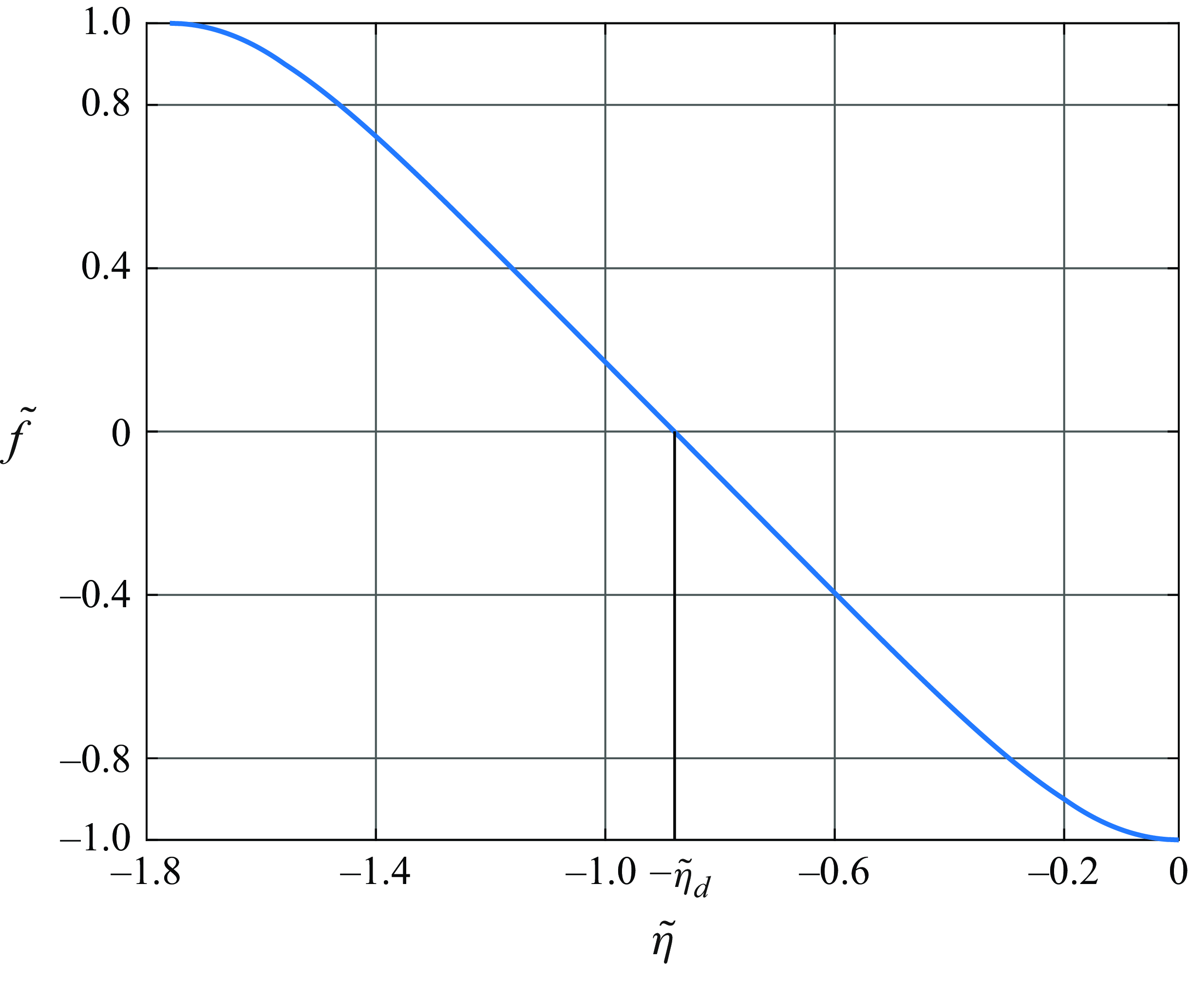
Figure 11. Function $\tilde {f} (\tilde {\eta })$
.
$\tilde {f} (\tilde {\eta })$
.
The choice of sign on the right-hand side of (5.39) depends on the flow region considered. We start with the flow below the Zero- $u$
-Line. In this region,
$u$
-Line. In this region, $\breve {u}$
is negative, and it follows from (5.21a
) and (5.31) that
$\breve {u}$
is negative, and it follows from (5.21a
) and (5.31) that ${\rm d} \tilde {f} / {\rm d} \tilde {\eta }$
is also negative. Hence, we write
${\rm d} \tilde {f} / {\rm d} \tilde {\eta }$
is also negative. Hence, we write
 \begin{equation} \frac {{\rm d} \tilde {f}}{{\rm d} \tilde {\eta }} = - \sqrt {2 \left ( 1 - |\tilde {f}|^{1/\alpha } \right ) } . \end{equation}
The initial condition for this equation is
 \begin{equation} \tilde {f} = - 1 \quad \text{at} \quad \tilde {\eta } = 0 . \end{equation}
The results of the numerical solution of the initial-value problem (5.40), (5.41) with $\alpha = 1/5$
are displayed in figure 11. Remember that the region below the Zero-
$\alpha = 1/5$
are displayed in figure 11. Remember that the region below the Zero- $u$
-Line corresponds to negative
$u$
-Line corresponds to negative $\tilde {\eta }$
. The solution may be formally extended from
$\tilde {\eta }$
. The solution may be formally extended from $\tilde {f} = - 1$
up to
$\tilde {f} = - 1$
up to $\tilde {f} = 1$
. However, only half of this solution with
$\tilde {f} = 1$
. However, only half of this solution with $\tilde {f} \in [-1, 0]$
is relevant to the flow considered here. Indeed, it follows from (5.19) that once
$\tilde {f} \in [-1, 0]$
is relevant to the flow considered here. Indeed, it follows from (5.19) that once $f$
turns zero, the stream function
$f$
turns zero, the stream function $\Psi$
appears to be constant and equals its value
$\Psi$
appears to be constant and equals its value $\Psi _s$
at the singular point
$\Psi _s$
at the singular point $S$
, thus giving us the lower boundary of the recirculation region. To deduce an explicit formula for the lower boundary, we denote the value of
$S$
, thus giving us the lower boundary of the recirculation region. To deduce an explicit formula for the lower boundary, we denote the value of $\tilde {\eta }$
at the point where
$\tilde {\eta }$
at the point where $\tilde {f} = 0$
as
$\tilde {f} = 0$
as
 \begin{equation} \tilde {\eta } = - \tilde {\eta }_d, \end{equation}
with $\tilde {\eta }_d \approx 0.8797$
. Then, it follows from (5.31) that at this point,
$\tilde {\eta }_d \approx 0.8797$
. Then, it follows from (5.31) that at this point,
 \begin{align} \eta = - \frac {|f (0)|}{\sqrt {\lambda }} \tilde {\eta }_d . \end{align}
Using (5.20), we further have
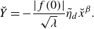 \begin{align} \breve {Y} = - \frac {|f (0)|}{\sqrt {\lambda }} \tilde {\eta }_d \breve {x}^{\beta } . \end{align}
It remains to return to the original coordinates (5.17) and we can conclude that
 \begin{equation} Y = Z (x) - \frac {|f (0)|}{\sqrt {\lambda }} \tilde {\eta }_d (x - x_s)^{\beta } . \end{equation}
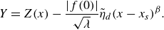
If, as before, we disregard the existence of the near-wall viscous layer and assume that the lower boundary of the reverse flow region lies along the body surface, then we can set $Y = 0$
in (5.45). As a result, we will find that the Zero-
$Y = 0$
in (5.45). As a result, we will find that the Zero- $u$
-Line is given by
$u$
-Line is given by
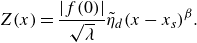 \begin{equation} Z (x) = \frac {|f (0)|}{\sqrt {\lambda }} \tilde {\eta }_d (x - x_s)^{\beta } . \end{equation}
The region above the Zero- $u$
-Line is studied in the same way and, in fact, the flow appears to be symmetric if considered in the coordinates
$u$
-Line is studied in the same way and, in fact, the flow appears to be symmetric if considered in the coordinates $(\breve {x}, \breve {Y})$
. More precisely, the stream function
$(\breve {x}, \breve {Y})$
. More precisely, the stream function $\breve {\Psi }$
is symmetric, while the longitudinal velocity components
$\breve {\Psi }$
is symmetric, while the longitudinal velocity components $\breve {u}$
is anti-symmetric. The outer edge of the recirculation region in
$\breve {u}$
is anti-symmetric. The outer edge of the recirculation region in $(x, Y)$
-coordinates is given by
$(x, Y)$
-coordinates is given by
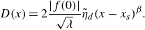 \begin{align} D (x) = 2 \frac {|f (0)|}{\sqrt {\lambda }} \tilde {\eta }_d (x - x_s)^{\beta } . \end{align}
Remember that $\beta$
is negative, which means that
$\beta$
is negative, which means that $Z (x)$
, as well as
$Z (x)$
, as well as $D (x)$
, decrease with
$D (x)$
, decrease with $x$
. This is in line with the numerical results shown in figure 9, where we observe a sharp drop of
$x$
. This is in line with the numerical results shown in figure 9, where we observe a sharp drop of $Z$
behind the singular point
$Z$
behind the singular point $S$
. Of course, the singularity predicted by (5.46) at
$S$
. Of course, the singularity predicted by (5.46) at $x = x_s$
could not be reproduced in the numerical solution (figure 9) as our finite-difference technique looses its accuracy near the singular point.
$x = x_s$
could not be reproduced in the numerical solution (figure 9) as our finite-difference technique looses its accuracy near the singular point.
5.3. Von Mises variables
To confirm the numerical prediction (5.27) for parameter $\alpha$
, it is convenient to use the von Mises variables. The momentum equation (2.5a
) is written in von Mises variables as
$\alpha$
, it is convenient to use the von Mises variables. The momentum equation (2.5a
) is written in von Mises variables as
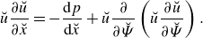 \begin{equation} \breve {u} \frac {\partial \breve {u}}{\partial \breve {x}} = - \frac {{\rm d} p} {{\rm d} \breve {x}} + \breve {u} \frac {\partial }{\partial \breve {\Psi }} \left ( \breve {u} \frac {\partial \breve {u}}{\partial \breve {\Psi }} \right ) . \end{equation}
It follows from (5.19), (5.21a
) that the solution to (5.48) immediately behind singular point $S$
should be sought in the form
$S$
should be sought in the form
 \begin{equation} \breve {u} = \breve {x}^{1/2} F (\xi ) + \cdots \quad \text{as} \quad \breve {x} \to 0^{+}, \end{equation}
where
 \begin{equation} \xi = \frac {\breve {\Psi } - \Psi _s}{\breve {x}^{\alpha }} . \end{equation}
Using (5.49), (5.50), we calculate the inertia and viscous terms in (5.48):
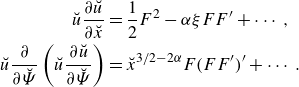 \begin{align} \breve {u} \frac {\partial \breve {u}}{\partial \breve {x}} &= \frac {1}{2} F^2 - \alpha \xi F F^{\prime } + \cdots, \nonumber \\ \breve {u} \frac {\partial }{\partial \breve {\Psi }} \left ( \breve {u} \frac {\partial \breve {u}}{\partial \breve {\Psi }} \right ) &= \breve {x}^{3/2 - 2 \alpha } F (F F^{\prime })^{\prime } + \cdots . \end{align}
If we assume, subject to subsequent confirmation, that
 \begin{equation} \alpha \lt \frac {3}{4}, \end{equation}
then we shall see that the viscous term in (5.48) may be disregarded. Keeping further in mind that the pressure gradient is given by (5.22d
), we can conclude that function $F (\xi )$
satisfies the equation
$F (\xi )$
satisfies the equation
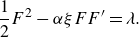 \begin{equation} \frac {1}{2} F^2 - \alpha \xi F F^{\prime } = \lambda . \end{equation}
The general solution of this equation is written as
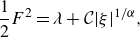 \begin{align} \frac {1}{2} F^2 = \lambda + \mathcal{C} | \xi |^{1/\alpha }, \end{align}
where $\mathcal{C}$
is an arbitrary constant. If we denote the value of
$\mathcal{C}$
is an arbitrary constant. If we denote the value of $\xi$
on the Zero-
$\xi$
on the Zero- $u$
-Line by
$u$
-Line by $\xi _0$
, then we can see that
$\xi _0$
, then we can see that $\mathcal{C} = - \lambda / | \xi _0|^{1/\alpha }$
, and therefore,
$\mathcal{C} = - \lambda / | \xi _0|^{1/\alpha }$
, and therefore,
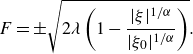 \begin{equation} F = \pm \sqrt { 2 \lambda \left ( 1 - \frac {| \xi |^{1/\alpha }}{| \xi _0|^{1/\alpha }} \right ) } . \end{equation}
The solution (5.55) applies to the flow on the right-hand side of the dividing streamline that passes through the singular point $S$
. On this streamline,
$S$
. On this streamline, $\breve {\Psi } = \Psi _s$
, while in the region considered,
$\breve {\Psi } = \Psi _s$
, while in the region considered, $\breve {\Psi } \lt \Psi _s$
, which means that
$\breve {\Psi } \lt \Psi _s$
, which means that $\xi$
, as defined by (5.50), is negative.
$\xi$
, as defined by (5.50), is negative.
Let us start with the flow below the Zero- $u$
-Line where
$u$
-Line where $u$
is negative, and therefore,
$u$
is negative, and therefore,
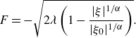 \begin{equation} F = - \sqrt { 2 \lambda \left ( 1 - \frac {| \xi |^{1/\alpha }}{| \xi _0|^{1/\alpha }} \right ) } . \end{equation}
To study the flow behaviour close to the dividing streamline, we set $|\xi | \to 0$
in (5.56). We find
$|\xi | \to 0$
in (5.56). We find
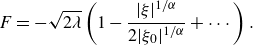 \begin{equation} F = - \sqrt {2 \lambda } \left ( 1 - \frac {|\xi |^{1 / \alpha }}{2 |\xi _0|^{1 / \alpha }} + \cdots \right ) . \end{equation}
Here,
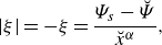 \begin{equation} |\xi | = - \xi = \frac {\Psi _s - \breve {\Psi }}{\breve {x}^{\alpha }}, \end{equation}
which, being substituted into (5.57), yields
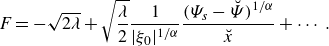 \begin{equation} F = - \sqrt {2 \lambda } + \sqrt {\frac {\lambda }{2}} \frac {1}{|\xi _0|^{1 / \alpha }} \frac {(\Psi _s - \breve {\Psi })^{1 / \alpha }}{\breve {x}} + \cdots . \end{equation}
It remains to substitute (5.59) into (5.49) and we find that the longitudinal velocity
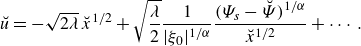 \begin{equation} \breve {u} = - \sqrt {2 \lambda } \,\breve {x}^{1/2} + \sqrt {\frac {\lambda }{2}} \frac {1}{|\xi _0|^{1 / \alpha }} \frac {(\Psi _s - \breve {\Psi })^{1 / \alpha }} {\breve {x}^{1/2}} + \cdots . \end{equation}
Using (5.60), one can see that the viscous term on the right-hand side of the momentum equation (5.48) is estimated as
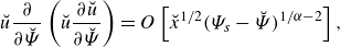 \begin{equation} \breve {u} \frac {\partial }{\partial \breve {\Psi }} \left ( \breve {u} \frac {\partial \breve {u}}{\partial \breve {\Psi }} \right ) = O \left [ \breve {x}^{1/2} (\Psi _s - \breve {\Psi })^{1 / \alpha - 2} \right ], \end{equation}
while the inertia term on the left-hand side of this equation
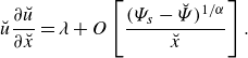 \begin{equation} \breve {u} \frac {\partial \breve {u}}{\partial \breve {x}} = \lambda + O \left [ \frac { (\Psi _s - \breve {\Psi })^{1 / \alpha }}{\breve {x}} \right ] . \end{equation}
Comparing (5.61) with (5.62), we can see that when $\Psi _s - \breve {\Psi }$
becomes an order
$\Psi _s - \breve {\Psi }$
becomes an order $O (\breve {x}^{3/4})$
quantity, the viscous term can no longer be disregarded, and a new viscous region should be introduced. Guided by (5.60), we seek the solution in this region in the form
$O (\breve {x}^{3/4})$
quantity, the viscous term can no longer be disregarded, and a new viscous region should be introduced. Guided by (5.60), we seek the solution in this region in the form
 \begin{equation} \breve {u} (\breve {x}, \breve {\Psi }) = - \sqrt {2 \lambda } \,\breve {x}^{1/2} + \breve {x}^{3/4\alpha - 1/2} Q (\zeta ) + \cdots \quad \text{as} \quad \breve {x} \to 0, \end{equation}
with
 \begin{equation} \zeta = \frac {\Psi _s - \breve {\Psi }}{\breve {x}^{3/4}} . \end{equation}
The condition of matching of (5.63) with (5.60) is written as
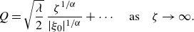 \begin{equation} Q = \sqrt {\frac {\lambda }{2}} \,\frac {\zeta ^{1 / \alpha }}{|\xi _0 |^{1 / \alpha }} + \cdots \quad \text{as} \quad \zeta \to \infty . \end{equation}
Substitution of (5.63) into (5.48) yields the following equation for $U (\zeta )$
:
$U (\zeta )$
:
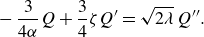 \begin{equation} - \frac {3}{4 \alpha } Q + \frac {3}{4} \zeta Q^{\prime } = \sqrt {2 \lambda }\, Q^{\prime \prime } . \end{equation}
To study the properties of this equation, it is convenient to perform the following substitution of variables:
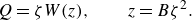 \begin{equation} Q = \zeta W (z), \qquad z = B \zeta ^2 . \end{equation}
If we choose constant $B = 3 / 8 \sqrt {2 \lambda }$
, then the equation for
$B = 3 / 8 \sqrt {2 \lambda }$
, then the equation for $W (z)$
takes the form
$W (z)$
takes the form
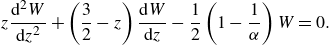 \begin{equation} z \frac {{\rm d}^2 W}{{\rm d} z^2} + \left ( \frac {3}{2} - z \right ) \frac {{\rm d} W}{{\rm d} z} - \frac {1}{2} \left ( 1 - \frac {1}{\alpha } \right ) W = 0 . \end{equation}
This is a confluent hypergeometric equation (see, for example, Abramowitz & Stegun Reference Abramowitz and Stegun1965) with parameters
 \begin{equation} a = \frac {1}{2} \left ( 1 - \frac {1}{\alpha } \right ), \qquad b = \frac {3}{2} . \end{equation}
Choosing two complementary solutions of (5.68) to be Kummer’s function $w_1 = M (a, b, z)$
and
$w_1 = M (a, b, z)$
and $w_2 = z^{1-b} M (1+a-b, 2-b,z)$
, we can write the general solution as
$w_2 = z^{1-b} M (1+a-b, 2-b,z)$
, we can write the general solution as
 \begin{equation} W = \mathcal{C}_1 M (a, b, z) + \mathcal{C}_2 z^{1-b} M (1+a-b, 2-b,z) . \end{equation}
Kummer’s function $M (a, b, z)$
is known to remain regular in the entire complex
$M (a, b, z)$
is known to remain regular in the entire complex $z$
-plane. In fact, it may be represented by the Taylor series
$z$
-plane. In fact, it may be represented by the Taylor series
 \begin{align} M (a, b, z) = \sum _{n=0}^{\infty } \frac {(a)_n}{(b)_n n!} z^n + \cdots, \end{align}
where $(a)_n$
denotes a quantity defined as
$(a)_n$
denotes a quantity defined as
 \begin{equation} (a)_0 = 1, \qquad (a)_n = (a + n - 1) (a)_{n-1} . \end{equation}
Clearly, the second complementary solution develops a singularity as $z \to 0$
, namely,
$z \to 0$
, namely, $w_2 = O (z^{-1/2})$
, and has to be disregarded since point
$w_2 = O (z^{-1/2})$
, and has to be disregarded since point $z = 0$
lies in the viscous region where the fluid dynamic functions should be smooth. Thus, we set
$z = 0$
lies in the viscous region where the fluid dynamic functions should be smooth. Thus, we set $\mathcal{C}_2 = 0$
, which reduces (5.70) to
$\mathcal{C}_2 = 0$
, which reduces (5.70) to
 \begin{align} W = \mathcal{C}_1 M (a, b, z) . \end{align}
Now, we need to look at the matching condition (5.65). Kummer’s function is known to exhibit the following behaviour:
 \begin{equation} M (a, b, z) = \frac {\Gamma (b)}{\Gamma (a)} e^z z^{a-b} + \cdots \end{equation}
as $z$
tends to infinity along a ray that lies in the right half (
$z$
tends to infinity along a ray that lies in the right half ( $\Re \{z\} \gt 0$
) of the complex plane
$\Re \{z\} \gt 0$
) of the complex plane $z$
. In our case,
$z$
. In our case, $z$
lies on the real positive semi-axis, making
$z$
lies on the real positive semi-axis, making $Q (\zeta )$
exponentially large for
$Q (\zeta )$
exponentially large for $\zeta \to \infty$
. This contradicts the matching condition (5.65) which requires
$\zeta \to \infty$
. This contradicts the matching condition (5.65) which requires $Q (\zeta )$
to grow algebraically. The contradiction is resolved by the fact that (5.74) cannot be used for
$Q (\zeta )$
to grow algebraically. The contradiction is resolved by the fact that (5.74) cannot be used for
 \begin{equation} a = - m, \qquad m = 0, \; 1, \; 2 \ldots, \end{equation}
when Gamma function $\Gamma (a)$
turns zero. If
$\Gamma (a)$
turns zero. If $a$
assumes one of the values in (5.75), then
$a$
assumes one of the values in (5.75), then $(a)_{m+1}$
and all the subsequent members of the sequence (5.72) vanish, reducing the Taylor series (5.70) to a polynomial of degree
$(a)_{m+1}$
and all the subsequent members of the sequence (5.72) vanish, reducing the Taylor series (5.70) to a polynomial of degree $m$
.
$m$
.
Remember that parameter $a$
is given by the first equation in (5.69). Using it on the left-hand side of (5.75), we find that for the problem considered, the set of eigenvalues is
$a$
is given by the first equation in (5.69). Using it on the left-hand side of (5.75), we find that for the problem considered, the set of eigenvalues is
 \begin{align} \alpha = \frac {1}{2 m + 1}, \qquad m = 0, \; 1, \; 2 \ldots . \end{align}
The first of these, $\alpha = 1$
, does not satisfy restriction (5.52) and should be discarded. Thus, the permissable eigenvalues are
$\alpha = 1$
, does not satisfy restriction (5.52) and should be discarded. Thus, the permissable eigenvalues are
 \begin{align} \alpha = \frac {1}{3}, \;\; \frac {1}{5}, \;\; \frac {1}{7}, \; \cdots \, . \end{align}
Returning back to the numerical evaluation (5.27) of $\alpha$
, we can see that in the flow considered,
$\alpha$
, we can see that in the flow considered,
 \begin{equation} \alpha = \frac {1}{5} . \end{equation}
6. Concluding remarks
This paper is concerned with a long-standing unresolved problem of the asymptotic theory of separated flow, the problem of the boundary-layer separation from an upstream moving wall. A major difficulty proved to be an unclear topology of the flow near the separation. To better understand what happens when the boundary layer separates on an upstream moving wall, we consider, as an example, the fluid flow on the leading edge of an aerofoil. Flow analysis is conducted in the framework of the classical Prandtl formulation. We first solve the boundary-layer equations numerically, for which purpose a new numerical technique was developed. The calculations were performed for a range of angles of attack and it was found that there exists a critical value of the angle of attack for which a Moore–Rott–Sears singularity forms in the flow. This is accompanied by an abrupt thickening of the boundary layer at the singular point and the formation of a recirculation region with closed streamlines behind this point. We found that the flow in this region may be treated as ‘almost inviscid’, which makes the Prandtl–Batchelor theorem applicable. Using this theorem, a rather simple theoretical model was offered to describe the flow.
We further found that the singular point does not belong to the Prandtl–Batchelor region but lies in front of it. The flow in the immediate vicinity of the singular point was studied in detail, first, using traditional formulation of the boundary-layer equations and then using von Mises variables. The solution with both formulations was obtained analytically in a self-similar form for the flow behind the singular point. Unfortunately, we still do not know how this solution can be extended to the region before the singularity. To demonstrate what happens with the boundary layer near singular point $S$
, we show in figure 12 the longitudinal velocity profiles,
$S$
, we show in figure 12 the longitudinal velocity profiles, $u (Y)$
, in a number of cross-sections on both sides of this point. One can see that
$u (Y)$
, in a number of cross-sections on both sides of this point. One can see that $u$
experiences a sharp change, perhaps a discontinuity, between cross-sections
$u$
experiences a sharp change, perhaps a discontinuity, between cross-sections $x = 1.58$
and
$x = 1.58$
and $x = 1.6$
. The existence of discontinuous solutions of the classical boundary-layer equations was first demonstrated by Ruban & Vonatsos (Reference Ruban and Vonatsos2008).
$x = 1.6$
. The existence of discontinuous solutions of the classical boundary-layer equations was first demonstrated by Ruban & Vonatsos (Reference Ruban and Vonatsos2008).
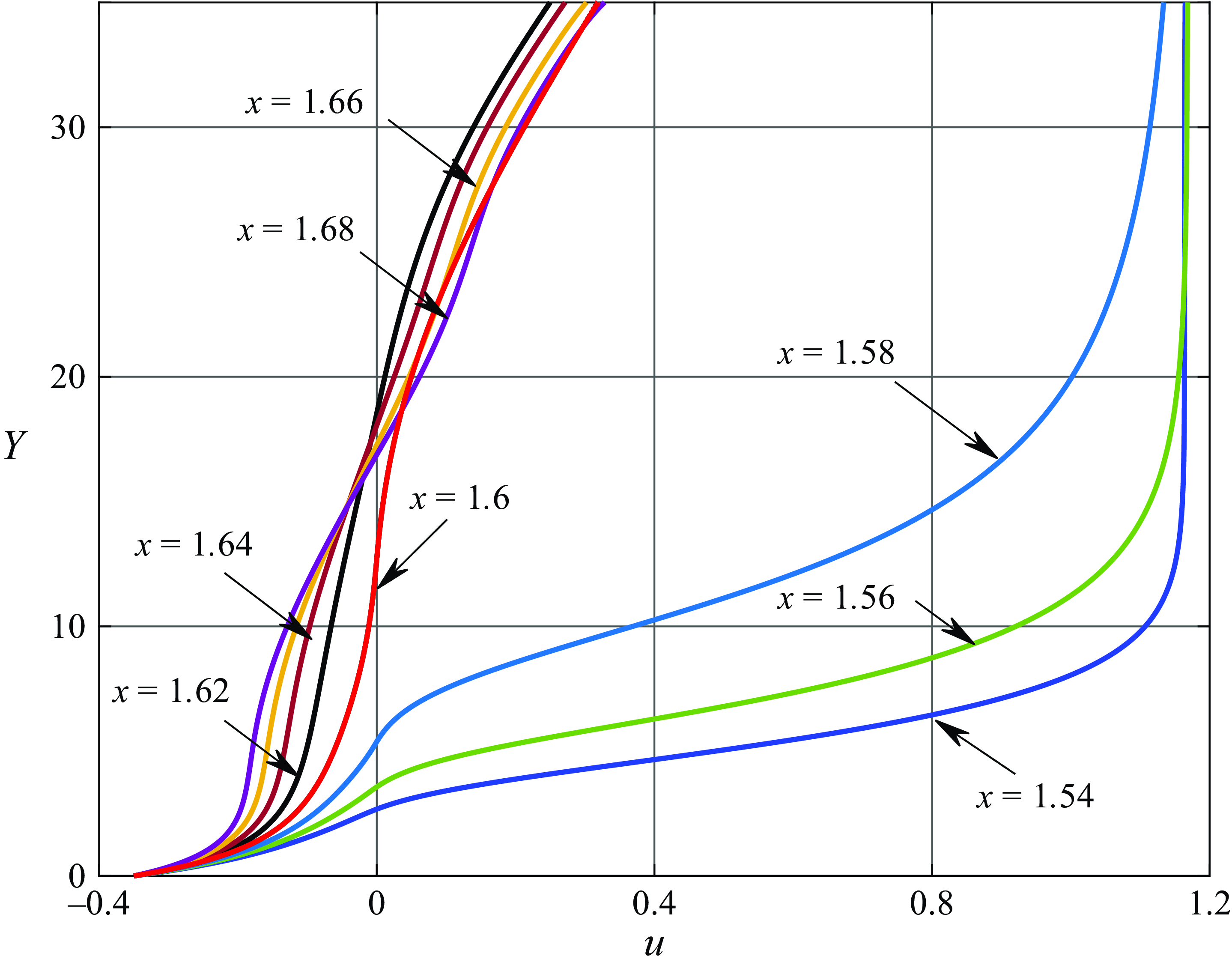
Figure 12. Longitudinal velocity profiles, $u (Y)$
, near the singularity.
$u (Y)$
, near the singularity.
A similar problem was studied earlier by Bezrodnykh et al. (Reference Bezrodnykh, Zametaev and Chzhun2023). These authors considered the boundary layer on a flat plate with upstream moving surface. The pressure perturbations in the boundary layer were produced by a dipole placed some distance above the plate. The solution of the boundary-layer equations were obtained using a numerical technique that was different from the one presented here. Of course, direct comparison of their results with the results presented in this paper is not possible. Still, we can see various qualitative similarities in the computational results, but there are significant differences in the theoretical description of the flows. In particular, Bezrodnykh et al. (Reference Bezrodnykh, Zametaev and Chzhun2023) found that parameter $\beta$
in (5.20) is positive, namely,
$\beta$
in (5.20) is positive, namely, $\beta = 1/6$
.
$\beta = 1/6$
.
Declaration of interests
The authors report no conflict of interest.
Appendix. Exact solution for the front stagnation point
In the case of a motionless wall, the flow near the stagnation point is described by one of the exact solutions of the boundary-layer equations as well as of the full Navier–Stokes equations, known as the Hiemenz (Reference Hiemenz1911) solution. Here, we shall generalise this solution to the case of a moving wall.
It follows from inviscid flow solution (2.1) that
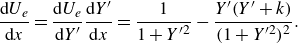 \begin{align} \frac {{\rm d} U_e}{{\rm d} x} = \frac {{\rm d} U_e}{{\rm d} Y^{\prime }} \frac {{\rm d} Y^{\prime }}{{\rm d} x} = \frac {1}{1 + Y^{\prime 2}} - \frac {Y^{\prime } (Y^{\prime } + k)}{(1 + Y^{\prime 2})^2} . \end{align}
In particular, at the front stagnation point,
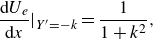 \begin{equation} \frac {{\rm d} U_e}{{\rm d} x}\Big| _{Y^{\prime } = - k} = \frac {1}{1 + k^2}, \end{equation}
which means that near this point,
 \begin{equation} U_e = \frac {1}{1 + k^2} \,x + \cdots \quad \text{as} \quad x \to 0 . \end{equation}
The flow in the boundary layer is described by (2.5), which should be solved with the boundary conditions (2.6). Let us assume that (A3) is valid for all finite values of $x$
. We then seek the stream function in the boundary layer in the form
$x$
. We then seek the stream function in the boundary layer in the form
 \begin{equation} \Psi (x, Y) = x f_0 (Y) + f_1 (Y) . \end{equation}
Substitution of (A4) into (2.7) yields
 \begin{equation} u = x f_0^{\prime } (Y) + f_1^{\prime } (Y), \qquad V = - f_0 (Y) . \end{equation}
Now, we substitute (A5) together with (A3) into (2.5a
). We find that (2.5a
) is satisfied provided that the functions $f_0 (Y)$
,
$f_0 (Y)$
, $f_1 (Y)$
satisfy the equations
$f_1 (Y)$
satisfy the equations
 \begin{align} &f_0^{\prime \prime \prime } + f_0 f_0^{\prime \prime } - \left ( f_0^{\prime } \right ) ^2 + \frac {1}{(1 + k^2)^2} = 0, \end{align}
 \begin{align} &\qquad\quad f_1^{\prime \prime \prime } + f_0 f_1^{\prime \prime } - f_0^{\prime } f_1^{\prime } = 0 . \end{align}
The boundary conditions for these equations are obtained by substituting (A5) into (2.6). We have
 \begin{align} f_0 (0) = f_0^{\prime } (0) &= 0, \quad\qquad f_0^{\prime } (\infty ) = \frac {1} {1 + k^2}, \end{align}
 \begin{align} f_1^{\prime } (0) &= U_w, \quad\quad\, f_1^{\prime } (\infty ) = 0 . \end{align}
Equation (A6a
) considered with boundary conditions (A7a
) represents the classical Hiemenz problem for the flow near the front stagnation on a motionless wall. The solution of this boundary-value problem may be found numerically. With known $f_0 (Y)$
, (A6b
) may be thought of as a second-order differential equation for
$f_0 (Y)$
, (A6b
) may be thought of as a second-order differential equation for $f_1^{\prime } (Y)$
. Its solution satisfying the boundary conditions (A7b
) can be written as
$f_1^{\prime } (Y)$
. Its solution satisfying the boundary conditions (A7b
) can be written as
 \begin{equation} f_1^{\prime } = \lambda f_0^{\prime \prime } (Y), \end{equation}
where constant $\lambda$
is given by
$\lambda$
is given by
 \begin{equation} \lambda = \frac {U_w}{f_0^{\prime \prime } (0)} . \end{equation}
Indeed, substitution of (A8) into (A6b ) results in
 \begin{equation} f_0^{\textrm {(iv)}} + f_0 f_0^{\prime \prime \prime } - f_0^{\prime } f_0^{\prime \prime } = 0 . \end{equation}
We know that $f_0 (Y)$
satisfies (A6a
) which, being differentiated with respect to
$f_0 (Y)$
satisfies (A6a
) which, being differentiated with respect to $Y$
, leads to (A10), which proves that the latter is indeed satisfied. The boundary conditions (A7b
) are verified by simply setting
$Y$
, leads to (A10), which proves that the latter is indeed satisfied. The boundary conditions (A7b
) are verified by simply setting $Y=0$
and
$Y=0$
and $Y=\infty$
in (A8), (A9).
$Y=\infty$
in (A8), (A9).
Integration of (A8) results in
 \begin{equation} f_1 = \lambda f_0^{\prime } (Y) + \mathcal{C}, \end{equation}
where $\mathcal{C}$
is a constant. Substitution of (A11) into (A4) allows us to express the stream function in the form
$\mathcal{C}$
is a constant. Substitution of (A11) into (A4) allows us to express the stream function in the form
 \begin{align} \Psi = x f_0 (Y) + \lambda f_0^{\prime } (Y) + \mathcal{C} . \end{align}
Of course, the stream function is defined to within an arbitrary constant. It is convenient to set $\mathcal{C} = 0$
and then we will have
$\mathcal{C} = 0$
and then we will have
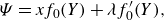 \begin{equation} \Psi = x f_0 (Y) + \lambda f_0^{\prime } (Y), \end{equation}
making $\Psi$
zero on the body surface.
$\Psi$
zero on the body surface.
We found $f_0 (Y)$
numerically. Once this was done, we used (A13) to determine the distribution of the stream function in the flow field. This allowed us to plot the streamline pattern for chosen values of
$f_0 (Y)$
numerically. Once this was done, we used (A13) to determine the distribution of the stream function in the flow field. This allowed us to plot the streamline pattern for chosen values of $k$
and
$k$
and $U_w$
. As an example, in figure 13, we show the streamline pattern for
$U_w$
. As an example, in figure 13, we show the streamline pattern for $k = 0$
and
$k = 0$
and $U_w = 2$
. It is interesting to notice that with the wall moving to the right, the fluid is not dragged directly to the right. Instead, a flow region is created where the fluid moves first to the left and then, closer to the wall, turns and starts moving to the right.
$U_w = 2$
. It is interesting to notice that with the wall moving to the right, the fluid is not dragged directly to the right. Instead, a flow region is created where the fluid moves first to the left and then, closer to the wall, turns and starts moving to the right.
Figure 13. Flow visualisation.
The streamline pattern for the wall moving to the left ( $U_w \lt 0$
) is obtained by a simple mirror-reflection in the
$U_w \lt 0$
) is obtained by a simple mirror-reflection in the $Y$
-axis.
$Y$
-axis.


 Open access