


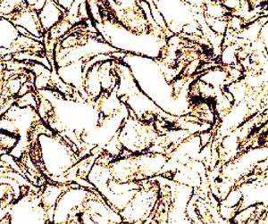



1. Introduction
Turbulent gas flows often harbour particles of different sizes, for example dust grains or water droplets. Larger particles can have significant inertia and decouple from the flow. This can lead to local enhancements of their density, which is generally described as clustering. This can be important for the coalescence of particles to larger ones. This process eventually leads to the formation of planetesimals in planetary accretion discs (Weidenschilling Reference Weidenschilling1980) or to raindrops in clouds (Shaw Reference Shaw2003; Grabowski & Wang Reference Grabowski and Wang2013). Another situation where particle clustering is important is when reactive particles are ‘competing’ for the same reactant gas. The concentration of reactant gas may then be significantly lower within a particle cluster than outside, which yields an overall lower reaction rate (Krüger, Haugen & Lovas Reference Krüger, Haugen and Lovas2017; Haugen et al. Reference Haugen, Krüger, Mitra and Løvås2018; Karchniwy, Klimanek & Haugen Reference Karchniwy, Klimanek and Haugen2019). For this situation, which is our main interest, it is large-scale clustering that is most important. The reason for this is that small particle clusters, of the order of the Kolmogorov scale, have a diffusive time scale that is shorter than the reactive time scale by which particles are consuming the reactant. For larger clusters, however, the particles will consume the reactant within the cluster faster than diffusion can transport fresh reactant to the cluster.
In clouds, and in most industrial applications, the compressibility of air is rather weak, because the turbulent flow speeds are strongly subsonic. This tends to be quite different in astrophysical flows such as those in accretion discs around young stars and the interstellar medium, which is continuously being fed with dust from the outflows of stars near the end of their lives. The driving of turbulence is fundamentally different in the meteorological and astrophysical contexts. Cloud turbulence is driven by convection, which is an intrinsically vortical flow. There is a large variety of turbulent industrial flows, but for the vast majority, the turbulence is typically driven by some sort of shear, which yields vortical flows. The interaction between inertial particles and shocklets in such compressible turbulent flows has been studied by Yang et al. (Reference Yang, Wang, Shi, Xiao, He and Chen2014), who found particle clustering near shocklets. Zhang et al. (Reference Zhang, Liu, Ma and Xiao2016) also found clustering near shocklets, but also noted clustering in regions of low vorticity for small Mach numbers due to the centrifuge effect. Turbulent flows with purely compressive driving are sometimes also referred to as acoustic (irrotational) turbulence or wave turbulence. Turbulence in the interstellar medium is driven predominately by supernova explosions, which are intrinsically compressive flows (see, e.g. Korpi et al. Reference Korpi, Brandenburg, Shukurov, Tuominen and Nordlund1999; Mac Low & Klessen Reference Mac Low and Klessen2004a; de Avillez & Breitschwerdt Reference de Avillez and Breitschwerdt2005; Federrath et al. Reference Federrath, Chabrier, Schober, Banerjee, Klessen and Schleicher2011; Gent et al. Reference Gent, Shukurov, Fletcher, Sarson and Mantere2013a,Reference Gent, Shukurov, Sarson, Fletcher and Mantereb, Reference Gent, Mac Low, Käpylä, Sarson and Hollins2020; Evirgen et al. Reference Evirgen, Gent, Shukurov, Fletcher and Bushby2019). At larger flow speeds, however, vorticity can always be produced by baroclinicity and shocks (Federrath et al. Reference Federrath, Chabrier, Schober, Banerjee, Klessen and Schleicher2011; Del Sordo & Brandenburg Reference Del Sordo and Brandenburg2011; Porter, Jones & Ryu Reference Porter, Jones and Ryu2015).
To isolate the distinctive properties of compressive and vortical turbulence, we simulate isothermal turbulence by applying a stochastic forcing that is either vortical or compressive. The assumption of isothermality is often made in the context of interstellar turbulence (Stone, Ostriker & Gammie Reference Stone, Ostriker and Gammie1998; Padoan & Nordlund Reference Padoan and Nordlund2002; Mac Low & Klessen Reference Mac Low and Klessen2004b), and can be motivated by short heating and cooling times. However, this justification may well be questioned, and we therefore regard isothermality as the simplest assumption to focus on the new effects of compressibility. Including physically motivated heating and cooling processes could lead to other new effects that are not specific to compressibility. For compressive forcing, the pressure enhancements, which are the result of energy injection of the forcing, are completely compressive. It is only when the resulting spherical expansion waves interact with each other that some vorticity can be produced – especially for large Mach number, which is the ratio of root-mean-square (r.m.s.) velocity to the sound speed. Likewise, the purely vortical driving can lead to significant compression and finite flow divergences at larger Mach numbers (see, e.g. Federrath et al. Reference Federrath, Chabrier, Schober, Banerjee, Klessen and Schleicher2011; Mattsson et al. Reference Mattsson, Bhatnagar, Gent and Villarroel2019a).
For purely acoustic turbulence, the energy spectra drop slightly more rapidly with wavenumber  $k$ (like $k^{-2}$) compared with the $k^{-5/3}$ Kolmogorov spectrum for vortical turbulence (Kadomtsev & Petviashvili Reference Kadomtsev and Petviashvili1973). Acoustic turbulence does not necessarily imply large Mach numbers, because the bulk speed may well be less than the wave speed. Owing to viscosity, purely irrotational flows cannot exist in reality and some level of vorticity will always be generated (Federrath et al. Reference Federrath, Chabrier, Schober, Banerjee, Klessen and Schleicher2011). Therefore, we prefer to talk about compressive turbulence instead. Our primary interest lies in the clustering of particles in these two types of flows for small and large Mach numbers.
There are two rather different approaches to simulating non-interacting inertial particles. One is to model them as a pressure-less fluid, and the other is to model them as non-interacting point particles. In both cases, the particles interact with the gas through friction. We refer to these two approaches as Eulerian and Lagrangian, respectively. Each of them has advantages and disadvantages. A Lagrangian description is ideal for dilute systems, but it is susceptible to statistical noise, especially at small length scales where there are fewer particles. This is a disadvantage of the Lagrangian approach. An important disadvantage of the fluid description is that it cannot describe how particles of the same type can go past each other. This is because in the fluid description one only considers the bulk flow, which is the average velocity of all particles of a specific type in a small local volume. The bulk velocity is therefore a single-valued function of position. In the Lagrangian description, by contrast, one does not average, and since there are usually several particles in every small volume, the flow velocity of the particle phase can be multi-valued. In particular, when particles go past each other, we have the formation of caustics. This implies that particles of the same size can have opposite velocities at the same location, creating phase-space singularities. In the Eulerian approach, this situation would lead to the formation of shocks – even for dilute particle populations. In the Lagrangian approach, by contrast, particle populations can go through each other without any interaction.
Caustic formation can be an important pathway to enhanced particle interaction (Wilkinson & Mehlig Reference Wilkinson and Mehlig2005; Bec et al. Reference Bec, Biferale, Lanotte, Scagliarini and Toschi2010; Gustavsson et al. Reference Gustavsson, Meneguz, Reeks and Mehlig2012; Voßkuhle et al. Reference Voßkuhle, Pumir, Lévêque and Wilkinson2014). This applies mainly to particles large enough to decouple from the carrier fluid and this phenomenon can be the main reason why such particles interact. At high Mach numbers, it is mainly shock interaction and compression of the carrier fluid when shocks meet that matters (Yang et al. Reference Yang, Wang, Shi, Xiao, He and Chen2014; Zhang et al. Reference Zhang, Liu, Ma and Xiao2016). This is because the density increase due to compression is by far the greatest effect.
A more commonly studied route to enhanced interaction rates is the centrifugal effect of turbulent eddies, which fling the particles to the edges of the eddies (Maxey & Riley Reference Maxey and Riley1983; Maxey Reference Maxey1987; Squires & Eaton Reference Squires and Eaton1991; Eaton & Fessler Reference Eaton and Fessler1994; Falkovich, Fouxon & Stepanov Reference Falkovich, Fouxon and Stepanov2002; Bec Reference Bec2003; Bec et al. Reference Bec, Biferale, Cencini, Lanotte, Musacchio and Toschi2007; Zaichik & Alipchenkov Reference Zaichik and Alipchenkov2009; Gustavsson & Mehlig Reference Gustavsson and Mehlig2011; Bragg & Collins Reference Bragg and Collins2014; Bragg, Ireland & Collins Reference Bragg, Ireland and Collins2015; Bragg Reference Bragg2017; Bhatnagar, Gustavsson & Mitra Reference Bhatnagar, Gustavsson and Mitra2018; Yavuz et al. Reference Yavuz, Kunnen, van Heijst and Clercx2018). This is because the particles do not experience the confining pressure that keeps the gas on closed streamlines. The relative importance of caustics and the centrifugal effects is not well understood (Voßkuhle et al. Reference Voßkuhle, Pumir, Lévêque and Wilkinson2014). One of the goals of the present study is therefore to assess their roles separately for vortical and compressively forced turbulence. This assessment will be based on the knowledge that caustics are only captured by the Lagrangian approach while the centrifugal effect is captured both by the Lagrangian and the Eulerian approaches.
The Lagrangian and Eulerian descriptions are complementary and can also be used to gauge their respective regimes of validity. This allows us to study, for example, when and at what length scales statistical noise becomes important, and when caustics formation becomes important. We focus on three-dimensional simulations, but we also use one-dimensional simulations, where caustic formation can be studied in isolation.
In both types of approaches, we ignore the back reaction of particles on the flow. This can become important at large mass loading parameters and can lead to other interesting effects such as the streaming instability (Johansen & Youdin Reference Johansen and Youdin2007) and the resonant drag instability (Squire & Hopkins Reference Squire and Hopkins2017), which will not be addressed here. We also neglect gravity and tidal forces.
To analyse particle clustering in incompressible turbulence, radial distribution functions (RDFs) have commonly been used (Sundaram & Collins Reference Sundaram and Collins1997; Reade & Collins Reference Reade and Collins2000; Wang, Wexler & Zhou Reference Wang, Wexler and Zhou2000; Salazar et al. Reference Salazar, De Jong, Cao, Woodward, Meng and Collins2008). They have also been used in the context of compressible transonic turbulence (Pan et al. Reference Pan, Padoan, Scalo, Kritsuk and Norman2011). Alternatively, one can use a spectral approach by calculating power spectra of particle densities. In the context of particle clustering, we only know of the work of Haugen et al. (Reference Haugen, Krüger, Mitra and Løvås2018), who have used power spectra of particle densities. This approach may be more suitable for characterising particle clustering at different length scales, including, in particular, scales larger than the Kolmogorov scale. Similar spectral quantities are known as structure factors in the context of crystallography (Jamieson, Abrahams & Bernstein Reference Jamieson, Abrahams and Bernstein1968), liquid metals (Ashcroft & Lekner Reference Ashcroft and Lekner1966) and biomolecular systems (Essmann et al. Reference Essmann, Perera, Berkowitz, Darden, Lee and Pedersen1995). The RDFs may be regarded as the real-space equivalents of these various spectral techniques; see the work of Shaw, Kostinski & Larsen (Reference Shaw, Kostinski and Larsen2002) which showed that these different measures can be related to each other; see also the textbook of McQuarrie (Reference McQuarrie2003). However, they can also be complementary to each other, as we shall show in this paper.
Contrary to earlier work on particle clustering, we are here interested in clustering at all scales, and not just the Kolmogorov scale. This seems particularly clear for particle clustering near shocklets, but may in fact also be true for inertial range clustering (Haugen et al. Reference Haugen, Krüger, Mitra and Løvås2018), which is due to classical vortex clustering at larger scales.
2. The model
We consider an isothermal gas where the pressure is proportional to the density  $\rho$ and is given by $\rho {c_{{s}}}^2$, with $ {c_{{s}}}$ being the isothermal sound speed. The velocity of the gas $\boldsymbol {u}$ is governed by the Navier–Stokes and continuity equations
 \begin{gather} \frac{\partial\boldsymbol{u}}{\partial t}+\boldsymbol{u}\boldsymbol{\cdot}\boldsymbol{\nabla}\boldsymbol{u}={-}{c_{{s}}}^2\boldsymbol{\nabla}\ln\rho + \boldsymbol{f} +\rho^{{-}1}\boldsymbol{\nabla}\boldsymbol{\cdot}(2\rho\nu{\boldsymbol{\mathsf{S}}}+\rho\zeta_{shock}{\boldsymbol{\mathsf{I}}}{\boldsymbol{\nabla}}\boldsymbol{\cdot}\boldsymbol{u}), \end{gather}
 \begin{gather} \frac{\partial\ln\rho}{\partial t}+\boldsymbol{u}\boldsymbol{\cdot}\boldsymbol{\nabla}\ln\rho ={-}\boldsymbol{\nabla}\boldsymbol{\cdot}\boldsymbol{u}, \end{gather}
where  $\boldsymbol {f}$ is a stochastic forcing term, $\nu$ is the kinematic viscosity, $\zeta_{\textit{shock}}$ is the shock viscosity, ${\boldsymbol{\mathsf{I}}}$ is the unit matrix with indices ${ {\mathsf {I}}}_{ij}=\delta _{ij}$ and ${\boldsymbol{\mathsf{S}}}$ is the trace-less rate of strain tensor with the components
 \begin{equation} { {\mathsf{S}}}_{ij}={\tfrac{1}{2}}(\partial u_i/\partial x_j+\partial u_j/\partial x_i) -{\tfrac{1}{3}}\delta_{ij}\boldsymbol{\nabla}\boldsymbol{\cdot}\boldsymbol{u}. \end{equation}
The forcing term consists either of random plane waves (vortical forcing) that are  $\delta$-correlated in time (Haugen et al. Reference Haugen, Kleeorin, Rogachevskii and Brandenburg2012), or of localised pressure enhancements (compressive forcing) with $\boldsymbol {f}=-\boldsymbol {\nabla }\phi$, where $\phi$ is a Gaussian in space at new locations in regular time intervals $\delta t_{f}$ (Mee & Brandenburg Reference Mee and Brandenburg2006). The amplitude of the forcing is denoted by $f_0$. For further details, we refer the reader to Appendix A.
In most of the simulations presented here, we perform direct numerical simulations (DNSs) in the sense that we solve the equations as stated. In those cases,  $\zeta _{shock}=0$. However, to save resources, especially in astrophysics, one often uses a shock-capturing viscosity (von Neumann & Richtmyer Reference von Neumann and Richtmyer1950). This broadens the shocks and allows one to resolve them on a coarser mesh. To assess the effect of such an artificial treatment on the particle clustering, in some cases we compare the results from the DNS with runs where a coarser mesh is used together with a shock-capturing viscosity. We adopt the shock-capturing viscosity of von Neumann & Richtmyer (Reference von Neumann and Richtmyer1950), which corresponds to a bulk viscosity with
 \begin{equation} \zeta_{shock}=C_{shock} \delta x^2 \langle-{\boldsymbol{\nabla}}\boldsymbol{\cdot}\boldsymbol{u}\rangle_+. \end{equation}
Here,  $\langle \cdots \rangle _+$ denotes a running five point average over all positive arguments, corresponding to a compression; see Caunt & Korpi (Reference Caunt and Korpi2001) and Haugen, Brandenburg & Mee (Reference Haugen, Brandenburg and Mee2004) for a detailed description. In contrast to the DNS, we refer to those simulations as large eddy simulations (LES).
It is important to realise that our Reynolds numbers are small compared with the many types of compressible flows occurring in nature. Therefore, our simulations are not DNS in a strict sense. Based on numerical considerations, the kinematic viscosity cannot be chosen too small. Therefore, we keep its value constant, which implies that the dynamic viscosity is enhanced in high density regions. On physical grounds, the dynamic viscosity tends to be more nearly constant, which would imply an enhanced kinematic viscosity in the regions of lower density outside shocks. This would have reduced the maximum permissible Reynolds number even further, and might have deprived us from finding effects related to higher Reynolds numbers.
In both the Lagrangian and Eulerian descriptions, the velocity  $\boldsymbol {v}_p$ of the particle with index $p$ couples to the gas through the friction force
 \begin{equation} \boldsymbol{F}_p={-}\frac{1}{\tau_p}(\boldsymbol{v}_p-\boldsymbol{u}). \end{equation}
It is assumed that the particles are smaller than the smallest turbulent eddies, which have sizes that are comparable to the Kolmogorov scale. For the flows considered here, the particle response time is given by a term that is slightly different for dense and dilute gases. When the mean-free path of the gas molecules is short, the response time is given by the Stokes time, modified by a Reynolds number-dependent factor of the form
 \begin{equation} \tau_p^{{St}}=\frac{2}{9}\, \frac{\rho_p}{\rho} \, \frac{a_p^2}{\nu} (1+0.15\,Re_{p}^{0.687})^{{-}1}, \end{equation}
where  $a_p$ and $\rho _p$ are the radius and material density, respectively, and $Re_{p} = a_{p}u_{rms}/\nu$ is the particle Reynolds number. Salazar et al. (Reference Salazar, De Jong, Cao, Woodward, Meng and Collins2008) used a similar approach to show that the results of their DNS were comparable to their experimental results of particle clustering in isotropic turbulence to within the limits of experimental uncertainty. For rarefied gases, the response time is based on the Epstein drag and is given by (Schaaf Reference Schaaf1963; Kwok Reference Kwok1975; Draine & Salpeter Reference Draine and Salpeter1979; Mattsson, Fynbo & Villarroel Reference Mattsson, Fynbo and Villarroel2019b)
 \begin{equation} \tau_p^{{Ep}}=\sqrt{\frac{\rm \pi}{8}}\frac{\rho_p}{\rho} \,\frac{a_p}{{c_{{s}}}}{\left(1+\frac{9{\rm \pi}}{128} \frac{{\left|\boldsymbol{u}-\boldsymbol{v}_p\right|}^2}{c_{{s}}^2}\right)}^{{-}1/2}. \end{equation}
The second term inside of the parenthesis becomes important at large Mach numbers.
In the Lagrangian description, the evolution of a particle  $p$ with velocity $\boldsymbol {v}_p$ at position $\boldsymbol {x}_p$ is given by
 \begin{equation} \frac{{\rm d}\boldsymbol{v}_p}{{\rm d}t}=\boldsymbol{F}_p,\quad \frac{{\rm d}\kern0.7pt\boldsymbol{x}_p}{{\rm d}t}=\boldsymbol{v}_p, \end{equation}
where we have ignored the effects of Brownian motion, which leads to the diffusion of particles. In the associated Eulerian description, diffusion is included and, instead of (2.8a,b), we solve instead
 \begin{gather} \frac{\partial\boldsymbol{v}_p}{\partial t}+\boldsymbol{v}_p\boldsymbol{\cdot}\boldsymbol{\nabla}\boldsymbol{v}_p=\boldsymbol{F}_p +\frac{2}{\rho_p}\boldsymbol{\nabla}\boldsymbol{\cdot}(\rho_p\nu_p{\boldsymbol{\mathsf{S}}}_p), \end{gather}
 \begin{gather} \frac{\partial n_p}{\partial t}+\boldsymbol{v}_p\boldsymbol{\cdot}\boldsymbol{\nabla} n_p ={-}n_p\boldsymbol{\nabla}\boldsymbol{\cdot}\boldsymbol{v}_p+\kappa_p\nabla^2 n_p, \end{gather}
where  $n_p$ is the particle number density and $\nu _p$ and $\kappa _p$ are artificial viscosity and diffusivity for the particle fluid (denoted now by $p$ collectively for all particles). Those terms are needed for reasons of numerical stability.
We use medium-resolution ( $N_{mesh}^3=256^3$ and $512^3$) in three-dimensional (3-D) triply periodic cubic domains with side lengths $L$ and the number of mesh points in each direction being $N_{mesh}$. The smallest wavenumber in the domain is then $k_1=2{\rm \pi} /L$. Unless otherwise specified, dust particles are included as inertial particles in five size bins with $4\times 10^6$ particles in each (for the Lagrangian simulations). We use the Pencil code (Pencil Code Collaboration 2021), which is a high-order, finite-difference code (sixth order in space and third order in time); see also Brandenburg & Dobler (Reference Brandenburg and Dobler2002) for details.
We sometimes also give the dimensional values of  $f_0$, $\delta t_{f}$, $\nu$, etc. Those are based on our choice $ {c_{{s}}}=2k_1=\langle \rho \rangle =1$ in the numerical calculations. In all cases, we use $\rho _{p}=10^3$.
3. Diagnostic tools
3.1. Non-dimensional numbers
The flow is characterised by the Reynolds and Mach numbers
 \begin{equation} Re=\frac{{u_{{rms}}}}{\nu{k_{{f}}}} \quad\text{and}\quad Ma=\frac{u_{rms}}{c_{s}}, \end{equation}
respectively, where  $ {k_{{f}}}$ is the forcing wavenumber. We also give the value of the Taylor microscale Reynolds number, $Re_\lambda =\lambda u_{1D}/\nu$, which is based on the Taylor microscale $\lambda =\sqrt {15\nu /\epsilon _{K}}$ and the 1-D r.m.s. velocity, $u_{1D}= {u_{{rms}}}/\sqrt {3}$. The behaviour of the particles is characterised by the Stokes numbers
 \begin{equation} St_{int}=\tau_{p}/\tau_{f} \quad\text{and}\quad St_{Kol}=\tau_{p}/\tau_{Kol}, \end{equation}
where  $\tau _p$ is the particle response time, $\tau _{f}=(u_{rms} {k_{{f}}})^{-1}$ is the time scale related to the size of large-scale fluid structures, e.g. the forcing scale, and $\tau _{Kol}=\sqrt {\nu /\epsilon _{K}}$ is the Kolmogorov time, where $\epsilon _{K}=\langle 2\rho \nu {\boldsymbol{\mathsf{S}}}^2\rangle$ is the energy dissipation rate. Both variants of the Stokes number are related to particle clustering due to particle inertia. For small Mach numbers, $\rho$ is close to the mean density $\bar {\rho }$, allowing us to express $\epsilon _{K}$ also in terms of the energy spectrum $E(k)$. They are normalised such that $\int E(k)\,{\rm d} k=\bar {\rho }\langle \boldsymbol {u}^2\rangle /2$. We then have $\epsilon _{K}=2\bar {\rho }\nu \int k^2 E(k)\,{\rm d} k$. Also of interest is the associated Kolmogorov scale $\ell _{Kol}=(\nu ^3/\epsilon _{K})^{1/4}$.
In the present work, we have defined  $\tau _{f}$ in terms of the wavenumber as $(u_{rms} {k_{{f}}})^{-1}$. An alternative definition would be in terms of the length scale $2{\rm \pi} / {k_{{f}}}$, which would make $\tau _{f}$ larger by a factor of $2{\rm \pi}$, and $St_{int}$ smaller by the same factor. This might be more meaningful, because it would result in a better representation of the actual separation between the Kolmogorov and integral scales, and hence a more correct ratio between $St_{int}$ and $St_{Kol}$. We should keep this in mind when comparing these numbers in the rest of the paper.
The Knudsen number of particles of a certain size is defined as the ratio of the mean-free path  $\lambda$ of the gas molecules to the size of the particle, i.e., $Kn=\lambda /d_{{p}}$. The drag force on the particles is inversely proportional to the particle response time; see (2.5). For a continuous fluid, where the Knudsen number is much smaller than unity, the particle response time is given by the Stokesian time; see (2.6). For rarefied gases, however, the mean-free path is large compared with the particle size and the response time is then given by the Epstein time, as given in (2.7).
The dimensionless particle size parameter (see Hopkins & Lee Reference Hopkins and Lee2016) is defined as
 \begin{equation} \alpha = \frac{\rho_{p}}{\langle\rho\rangle} \frac{a_{p}}{L_{f}}, \end{equation}
where  $L_{f}$ is taken to be the physical forcing scale of the turbulent flow. For small values of $Kn$, we find that the mean Stokes number is
 \begin{equation} \langle St_{int}\rangle = \frac{\langle \tau_p^{St}\rangle}{\tau_{f}} \approx \frac{(2/9)\,\alpha\,Re_p}{1+0.15\,Re_p^{0.687}} \sim \alpha\,Re_p, \end{equation}
while in the Epstein limit we find
 \begin{equation} \langle St_{int}\rangle = \frac{\langle\tau_p^{Ep}\rangle}{\tau_{f}} \approx \sqrt\frac{\rm \pi}{8}\,\alpha\,\mathcal{M}_{rms}\, \left(1+\frac{9{\rm \pi}}{128} \frac{\left|\boldsymbol{u}-\boldsymbol{v}_p\right|^2}{c_{{s}}^2}\right)^{{-}1/2}\sim \alpha\,\mathcal{M}_{rms}. \end{equation}
From these two relations one can see that, while  $St_{int}$ for a given particle size in the Epstein limit is mainly affected by compression and essentially unaffected by viscosity of the carrier fluid, it is inversely proportional to the viscosity in the Stokes limit.
3.2. Power spectra of particle density
To measure preferential clustering at all scales, from the smallest scale resolved in the simulation to the size of the simulation box, we compute power spectra of  $n_p$ as (Haugen et al. Reference Haugen, Krüger, Mitra and Løvås2018)
 \begin{equation} P_{n}(k)=\frac{1}{2} \sum_{k-\delta k/2 \leq |\boldsymbol{k}|< k+\delta k/2} \left|\hat{n}_p(\boldsymbol{k})\right|^2\,\text{d}^3\boldsymbol{k}, \end{equation}
where  $\hat {n}_p(\boldsymbol {k})={\mathcal {F}} ( n_p(\boldsymbol {x}) )$ is the Fourier transform of $n_p$, $\boldsymbol {k}=(k_x,k_y,k_z)$ is the wavevector, and the integration is over concentric shells in wave number space. From the above, we see that
 \begin{equation} \int_{k_1}^{k_{max}} P_{n}(k)\,{\rm d} k=\frac{1}{2}\langle n_p^2\rangle, \end{equation}
where  $k_{max}=k_1 N_{mesh}/2$ is the Nyquist wavenumber, and angle brackets, $\langle \cdots \rangle$, represent spatial averaging, which means that $\langle n_p^2\rangle ^{1/2}$ is the r.m.s. particle number density.
If the particles were randomly distributed,  $|\hat {n}_p(\boldsymbol {k})|$ would be on average independent of $k=|\boldsymbol {k}|$. In three dimensions, however, the shell integration introduces an additional $k^2$ factor, so we expect
 \begin{equation} P_{n}(k)=A k^2, \end{equation}
which can be combined with (3.7) to yield
 \begin{equation} \frac{1}{2} \langle n_p^2\rangle = \int_{k_1}^{k_{max}} A k^2\, {\rm d} k = \frac{A}{3}(k_{max}^3-k_1^3) \approx \frac{A}{3} k_{max}^3, \end{equation}
where we have assumed  $k_1\ll k_{max}$, and $A$ is a constant that we shall be concerned with later in § 4.2.2. We improve on this description further below, when we analyse concrete examples.
3.3. Definition of the RDFs
To put our results into the context of other commonly used tools of characterising particle clustering, we compare the results from our spectral analysis with the corresponding RDFs. They are defined as (Sundaram & Collins Reference Sundaram and Collins1997; Reade & Collins Reference Reade and Collins2000; Wang et al. Reference Wang, Wexler and Zhou2000; Salazar et al. Reference Salazar, De Jong, Cao, Woodward, Meng and Collins2008)
 \begin{equation} g(r_i)=\frac{N_i}{N}\left/\frac{4{\rm \pi} r_i^2\, \delta r}{4{\rm \pi} R^3/3},\right. \end{equation}
where  $N_i$ is the number of particle pairs separated by a distance $r_i\pm \delta r/2$, $N=N_p(N_p-1)/2$ is the total number of particle pairs, $N_p$ is the number of particles and $R$ is the largest radius that fits into the domain.
4. Results
In this paper, we are concerned with the differences in particle clustering between vortical and compressive forcings. To convey an impression of this phenomenon, we begin by showing in figure 1 the projected particle number densities of snapshots from DNSs with vortical and compressive forcings for Stokes numbers around unity. Evidently, the visual impressions for the two types of flow are rather different. Even though the typical length scales of the forcings are similar in the two cases, the clustering phenomenon is markedly different. For vortical forcing, the overall contrast between minimum and maximum particle concentrations is much smaller than for compressive forcing. In the vortical case, the particle concentrations take a more filamentary and perhaps sheet-like structure, while in the compressive case, the particle concentrations are more spherical in shape.

Figure 1. (a) Projected particle number density in a snapshot from a DNS with vortical forcing (later referred to as Run V2). (b) The same from a DNS with compressive forcing (later referred to as Run C2). Both cases correspond the particle size showing the most clustering ( $St_{int}=0.31$ and $0.36$, respectively).
4.1. One-dimensional simulations
To illustrate the effects specific to compressive clustering, let us consider first a 1-D shock model as an illustrative example. Here, we also compare the Lagrangian particle simulations with the ones in the Eulerian description.
4.1.1. Applicability of the Eulerian approach
Caustics formation in the particle distribution, which is evident from the presence of multi-valued particle velocities, is a phenomenon that cannot be described with the Eulerian approach; see Boffetta et al. (Reference Boffetta, Celani, DeLillo and Musacchio2007) and Shotorban & Balachandar (Reference Shotorban and Balachandar2009) for detailed comparisons. For small enough particle inertia, i.e. for small Stokes numbers, the Eulerian and Lagrangian approaches should agree with each other. However, there is also another source of discrepancy. The Lagrangian approach is suitable for modelling dilute systems, but, due to the finite number of particles, it also has the disadvantage of suffering from statistical fluctuations when the intention is to model non-dilute systems, where fluctuations should be small. Statistical noise does not occur in the Eulerian approach. Thus, for dense systems and small Stokes numbers, the Eulerian approach can be beneficial. To determine the limits of applicability of the Eulerian approach quantitatively, we consider a simple 1-D model.
We adopt a localised hump in the fluid density, which we model by a Gaussian in  $\ln \rho (x)$ at the position $x=0$ in a domain of size $-{\rm \pi} /2< x<3{\rm \pi} /2$. Thus, we take
 \begin{equation} \ln\rho[(x)/\rho_0]={\mathcal{A}} \exp ({-}x^2/2\sigma_s^2), \end{equation}
where  ${\mathcal {A}}$ is an amplitude factor, $\rho _0$ is an overall normalisation coefficient, the width is given by $\sigma =0.35$ and the ratio of the peak value over the background is 3.1. For these simulations we use periodic boundary conditions. The initial density profile launches an acoustic wave; see figure 2 for plots of $u_x$ and $\rho$ at $t=0.1$ and $t=0.5$. The front speed exceeds the sound speed when the gas speed approaches a certain fraction of the sound speed; see appendix B for an illustration. We then use the gas velocity and gas density at $t=0.5$ as initial condition for the particles by setting the particle velocity for all particle sizes equal to the fluid velocity. The particle number density of all particle sizes is set proportional to the gas density.

Figure 2. (a) Gas velocity and (b) density at  $t=0.1$ (upper row) and $t=0.5$ (lower row) in panels (c,d). The data for $t=0.5$ serve as initial condition for the particles.
In figure 3 we show the particle velocities as a function of position for Lagrangian and Eulerian models for particle radii  $a_p=3\times 10^{-3}$ and $10^{-1}$ at different times. We also show the gas velocity, which propagates at a speed slightly faster than the sound speed, $ {c_{{s}}}=1$; see Appendix B for a plot showing the numerically obtained dependence of the front speed on the gas speed. The lighter particles follow the fluid and are not shown, but the heavier ones lag behind because they only inherit the speed of the gas at $t=0.5$, and they are too heavy to get accelerated by the passing acoustic wave. At early times ( $t=1$), the velocities in the Lagrangian and Eulerian models are close to each other, but at later times the particle velocities in the Lagrangian description become multi-valued, which corresponds to caustics formation. This phenomenon becomes more prominent for the heavier particles since they are not decelerated by the drag from the gas. In the Eulerian description, we instead see the formation of a shock. Away from the shock, the Lagrangian and Eulerian descriptions agree with each other rather well, especially for the heavier particles. To resolve the shock in the Eulerian simulations, we must apply a certain amount of artificial viscosity and diffusivity for the particle fluid. If this artificial viscosity is too small, wiggles occur in the downstream part of the shock, as can already be seen from the profile of $v_x(x)$ in figure 3. Including such artificial viscosity and diffusivity is a purely numerical device to stabilise the solution, but it is likely to introduce errors in the results. By comparing with the Lagrangian approach, we will try to assess the extent of such artifacts.

Figure 3. Particle velocity in the Lagrangian simulation (solid black) and the Eulerian one (solid red), together with the gas velocity (dashed blue) at times  $t=1$, 2 and 3 for $a_p=3\times 10^{-3}$ (corresponding to $St_{int}=1$, panels a,c,e) and $10^{-1}$ (corresponding to $St_{int}=30$, panels b,d,f).
Snapshots of the particle number densities are shown in figure 4 for the same times and the same two particle sizes as in figure 3. We see the development of extended structures with two enhancements on their flanks, characteristic of caustics, as is correctly reproduced with the Lagrangian approach. The Eulerian approach, on the other hand, yields just a single albeit very strong spike, which may cause an increase of the particle-interaction rate even without any caustics forming.

Figure 4. Particle density in the Lagrangian simulation (solid black) and the Eulerian one (solid red), together with the gas density (dashed blue) at times  $t=1$, 2 and 3. Two particle sizes are shown: $a_p=3\times 10^{-3}$ (a,c,e) and $10^{-1}$ (b,d,f).
It is of interest to determine the Stokes number relevant for caustics formation. This is important for knowing the maximum Stokes number for which the Eulerian approximation can still be used. For smaller Stokes numbers, no artificial particle viscosity and diffusivity are needed. For larger Stokes numbers, however, the Eulerian approach can represent the caustics only as shocks, which requires an increasing amount of artificial viscosity and diffusivity to keep them numerically resolved. The Stokes number is defined through (3.2a,b). For the solution shown in figure 3, we find that the fluid travel time across the width of the front  $\Delta x$ is
 \begin{equation} \tau_{f}=\Delta x/\Delta u, \end{equation}
where  $\Delta u$ is the fluid velocity at the front. For the current experiments, $\Delta x$ is taken to be the thickness of the front at the time when the particles were introduced in the simulation; see Run A in table 1 for more details about the particles.

In the example discussed above, we have  $\tau _{f}=0.72/0.66\approx 1.1$, and we find caustics for $a_{p}\ge 10^{-3}$, which corresponds to $p=3$. To compute the critical Stokes number $St_{crit}$ above which caustics formation occurs, we need to know the $\rho _{p}/\rho$ ratio, where we take the fluid density on the upstream side of the front, which is here $\rho \approx 1.8$. We used $\rho _{p}=10^3$, so, altogether, we have $St_{crit}=0.30$. This means that, for simulations where the Stokes number is larger than $\sim 0.3$, the Eulerian particle approach cannot be used. It is important to realise that we are here talking about the Stokes number based on the largest fluid scale, $St_{int}$, and not the Kolmogorov scale. As we shall see below, at the numerical resolutions accessible in our 3-D simulations, the difference between $St_{int}$ and $St_{Kol}$ is not very large.
4.1.2. A mechanism for compressive supersonic clustering
The preferential particle concentrations near shocklets in compressible turbulent flows found and discussed by Yang et al. (Reference Yang, Wang, Shi, Xiao, He and Chen2014) and Zhang et al. (Reference Zhang, Liu, Ma and Xiao2016) suggest that irrotational supersonic flows can yield new ways of clustering that would not occur in vortical subsonic flows. One idea for such a mechanism is that particles of a suitable mass that move toward each other on two colliding shocks, will be decelerated as the shocks collide, but the particles are too heavy to become re-accelerated as the shocks depart again immediately after the collision. The particles will then be left behind after the shocks move away, forming a cluster. To test this idea, we use an experiment similar to that described in § 4.1.1, but with a stronger density enhancement.
We emphasise that the particle acceleration is always due to the drag on the particles because of the relative velocity difference between the particles and the fluid. However, the drag becomes stronger when the density is high; see (2.6) and (2.7), so the density also plays a role.
In § 4.1.1, we used the gas velocity and density at a certain time to reinitialise the particles by setting the particle velocity for all particle sizes to a value equal to the fluid velocity. The initial width of the density distribution is again  $0.35$. However, the density enhancement of the gas is now so strong that its distribution is so different from a Gaussian that it can no longer be used for reinitialising the particles in a simple way. We therefore reinitialise the fluid density equal to the density of the lightest particles and then set the density and velocity of the heavier particles to the same as the lightest particles. The ratio of the peak value of the density over its background then turns out to be 22. In this experiment, we only use the Lagrangian approach. See Run B in table 1 for more details about the particles.
The result of this experiment is shown in figure 5, where we plot  $xt$ diagrams of $\rho$ and $n_p$ for different particle sizes. For small particles with small Stokes numbers, the particles follow the gas. This can be seen by the similarity between panels (a,b). To estimate $St_{int}$ in this case, we used $\Delta u=2.6$ and $\Delta x=0.08$, so $\tau _{f}=0.08/2.6\approx 0.03$. For our largest particles with $a_{p}=0.1$, we find $\rho \approx 300$; see the blue lines in figure 6. We again used $\rho _{p}=10^3$, which yields $\rho _{p}/\rho =1000/300\approx 3$. Therefore, $\tau _{p}=\sqrt {{\rm \pi} /8}\,(\rho _{p}/\rho )(a_{p}/ {c_{{s}}})\approx 0.2$, so we have $St_{int}\sim 7$.

Figure 5. The  $xt$ diagrams of (a) $\rho$, (b) $n_1$, (c) $n_4$, (d) $n_5$, (e) $n_6$ and (f) $n_7$. Dark shades indicate high densities. Note that shock clustering is most evident in panel (e).

Figure 6. Velocity of particles with radius  $a_6$ (black dots) and fluid velocity (red lines), as well as the gas density (blue lines and axes on the right) at $t=1.18$ (a), close to the time $t_*=1.16$ when the shocks meet and the gas density develops a peak. Panels (b,c) show the same at $t=t_*+\tau _6=1.22$ and $t_*+2\tau _6=1.28$.
For our largest particle size with  $St_{int}\approx 7$, the two counter-streaming particle clouds associated with the two opposing shocks tend to run through each other owing to their large inertia, as we can see from figure 5(f). For the intermediate size, where $St_{int}\approx 2$, however, a sizeable particle cloud is left behind at the original position of the collision of the two shocks; see figure 5(e). This critical value is close to unity, as one might have expected. We conclude from this that a particle cluster will form after the collision of two shocks if the Stokes number is around unity. Here, the Stokes number is based on the width and speed of the shock fronts. This mechanism for particle clustering is fundamentally different from the classical eddy mechanism of Maxey & Riley and it operates only for large enough Mach numbers. For such flows, however, it may be the dominating mechanism.
The biggest uncertainty in our estimate of  $St_{int}$ lies in the value of $\rho$. In the following, we focus on the particles in bin 6, and denote the corresponding velocity by $v_6$ and the response time of those particles by $\tau _6$. To determine the relevant value of $\rho$, we show in figure 6 the profiles of $\rho (x)$ together with those of $v_6(x)$ and $u(x)$ at times $t_*+\tau _6/3$, $t_*+\tau _6$ and $t_*+2\tau _6$, where $t_*=1.16$ is the time when the shocks meet and the gas density develops a peak. We see that the peak in $\rho$ reaches values of around 400, but at the time $t_*+\tau _6$, the particles will have slowed down considerably. Therefore, the relevant density to be used is the temporally averaged density at the peak until that time, which is below 300.
4.2. Three-dimensional simulations
In this section, we present our main result concerning the detection of two separate clustering mechanisms through the Stokes number dependence of the spectral particle number density. Before presenting this, we discuss several peripheral aspects of the problem: we first demonstrate that the effect of statistical noise on the power spectra can be eliminated and we show how the results depend on the Reynolds number. We also show that the results are insensitive to the choice of the drag law (Stokesian vs Epstein drag). The Eulerian approach is only used to determine its limits of applicability at small Stokes numbers and the lack of agreement at larger ones. We finish with a demonstration of the artifacts caused by using a shock viscosity, which is avoided in the bulk of this paper.
4.2.1. Overview of the different runs
In the previous sections, we studied several aspects of particle clustering in idealised 1-D simulations. We will now proceed by turning our attention to fully 3-D turbulence simulations. As described in § 2, two kinds of forcings are employed in this work. In table 2, run names starting with ‘V’ use vortical forcings, while those starting with ‘C’ adopt spherical expansion wave forcing (compressive forcing). The numbers behind those letters indicate different forcing strengths, which yield different Mach numbers. Different Reynolds numbers are indicated by letters a and b. We also list the ranges  $[St_{int}^{min},St_{int}^{max}]$ and $[St_{Kol}^{min},St_{Kol}^{max}]$ of Stokes numbers, as defined in (3.2a,b). The run with Stokes drag is denoted by the letter S at the end. We also compare with corresponding Eulerian models (table 3), where we have included an artificial viscosity and diffusivity needed to stabilise the simulations; see (2.9) and (2.10). For simulations with larger Mach numbers, the mesh must be refined in order to resolve the shocks. This means that the mesh spacing is significantly smaller than the Kolmogorov scale and, hence, that the Reynolds number must be decreased in order to confine the computational cost.
Table 2. Summary of our simulations; ‘comp’ and ‘vort’ refer to compressive and vortical forcings, respectively.

Table 3. Summary of Eulerian runs. For all these runs, the artificial diffusivity ( $\kappa _p$) equals the artificial viscosity ( $\nu _p$).

Contour plots of particle number density are shown in figure 7 for Run V2b. The different panels correspond to different Stokes numbers. It is clearly seen that the clustering is strongest for our intermediate Stokes numbers,  $St_{int}=0.33$ and $3.3$; see figure 7(b,c). For the very smallest and largest Stokes numbers, we see almost no clustering; see figure 7(a,d). In those cases, the values of $\alpha$ are 0.7 and 7, respectively, where we have used $L_{f}= {k_{{f}}}^{-1}$.

Figure 7. Contour plots of particle number density for (a)  $St_{int}=$ 0.033, (b) 0.33, (c) 3.3 and (d) 33 for case V2b. Dark shades denote high densities. The particle number density has been integrated over the perpendicular direction for four mesh zones.
In figure 8, we show scatter plots of the particle number density as a function of fluid density for all fluid grid cells in the domain. In (a), showing results for the smallest Stokes numbers, we see that there is a strong correlation between the two. This is because these small particles follow the fluid almost perfectly, which means that, when the fluid is compressed (high fluid density), the particle field is also compressed (high particle number density). When the Stokes number is increased, but is still rather small, we see in figure 8(b) that the two fields are only weakly correlated. Finally, for those Stokes numbers where we see the strongest clustering in figure 7(b), we show in figure 8(c) that there is no correlation between particle and fluid densities. We can also see the effect of the inertial clustering itself in that there is a large number of grid cells without any particles ( $n_p=0$), while there is also a significant number of grid cells containing many particles ( $n_p > 2$), which is not the case for the smaller Stokes numbers.

Figure 8. Scatter plot of particle number density as a function of fluid density for the three smallest particle sizes of case V2b. The solid line denotes the diagonal.
4.2.2. Kinetic energy and density power spectra
In this paper, we make extensive use of particle power spectra. In this context, it is useful to show first the relevant spectra for the gas. In figure 9, we show kinetic energy spectra together with power spectra of the gas density for cases V1, V2, C1 and C2. The peak of the kinetic energy spectrum occurs at  $k/k_1=3$ for the cases with vortical forcings (V1 and V2). This wavenumber indicates where the main power of the external forcing is found. For the cases with compressive forcing, however, the peak in the kinetic energy spectrum is found for $k/k_1$ between 1 and 2. The density power spectra follow the kinetic energy spectra fairly well, although there is a vertical shift. For the compressive forcing, we are driving strong flow divergencies, which results in $P_\rho (k)$ being large compared with $E_{K}(k)$. Since the vortical forcing is divergence free, the corresponding density variation is small, as seen through the smaller values of $P_\rho (k)$ compared with $E_{K}(k)$. We can also see that the extent of the vertical shift is larger for smaller Mach numbers. This is because the fluid is less compressed for smaller Mach numbers.

Figure 9. Values of  $E(k)$ (solid lines) and $P_\rho (k)$ (dashed lines) for our main cases (V1, V2, C1 and C2).
4.2.3. Initial and tracer particle spectra
In the following, we study power spectra of particle number densities for particles that are embedded in a fluid where turbulence is generated either with vortical or compressive forcing (Runs V1–V3 and Runs C1–C2, respectively). Since particles are tracked in a Lagrangian fashion, it is convenient to allocate each Lagrangian particle to the nearest Eulerian neighbours in each direction in the fluid mesh. In this way, for every particle size, we generate a variable on the fluid mesh that contains the number of particles that reside within or in the neighbourhood of a given grid cell. These variables can now be used to calculate the particle power spectra for each particle size. The size of the neighbourhood of grid cells that will be influenced by a given particle depends on the interpolation scheme used, which in our case is a second-order linear scheme (Johansen et al. Reference Johansen, Oishi, Mac Low, Klahr, Henning and Youdin2007).
Initially, the particles are randomly distributed over the entire simulation box. This means that the initial power spectra for the different particle sizes are just white noise, which corresponds to a  $k^2$ spectrum; see § 3.2. If every particle is associated solely with the very nearest grid point of the Eulerian mesh, the $k^2$ scaling would then be valid for the full wavenumber range. For the current work, however, the contribution from a particle is distributed over several nearby grid points through a linear interpolation scheme. This means that the $k^2$ scaling will not extend all the way to the largest wavenumbers. Instead, for $k>k_\ast$, the spectrum, hereafter $P_{{n},{noise}}$, becomes less steep and eventually reaches a maximum, before it goes down towards the very end.
In analogy with (3.9), we now get
 \begin{equation} \frac{1}{2} \langle n_p^2\rangle = \int_{k_1}^{{k}_{max}} P_{{n},{noise}}(k)\,{\rm d} k = \int_{k_1}^{{k}_{max}} A\tilde{k}^2\,{\rm d} k \equiv \frac{A}{3}\tilde{k}_{eff}^3, \end{equation}
where  $\tilde {k}=k/[1+(k/k_\ast )^3]$ has been substituted for $k$ in order to account for the departure from $k$ for $k\gtrsim k_\ast \equiv \kappa k_{max}$, with $\kappa \approx 0.789$ being a parameter proportional to the position of the local maximum of $P_n(k)$. This implies that $P_{{n},{noise}}=A\tilde {k}^2$. Defining therefore $\kappa =k_\ast /k_{max}$, we find $\tilde {k}_{eff}^3= (1+\kappa )(1-\kappa +\kappa ^2)/\kappa ^3k_{max}^3\approx {(1.45\,k_{max})^3}$. By re-arranging the above equation, the constant $A$, defined in § 3.2, is found to be $A=3(\langle n_p^2\rangle /2)/\tilde {k}_{eff}^3 \approx 0.49\langle n_p^2\rangle /k_{max}^3$. Together with (3.8) we then obtain the initial power spectrum of the particles as
 \begin{equation} P_{{n},{noise}}\approx 0.49\,\frac{\langle n_p^2\rangle B^2}{k_{max}^3}\tilde{k}^2, \end{equation}
where the constant on the right-hand side is defined as  $B=\langle \rho \rangle /\langle n_p\rangle$ and is introduced to compensate for the fact that the fluid and particle density fields do not have the same mean value. This compensation is required in order to obtain (4.5).
Particles that are very small, having essentially vanishing Stokes numbers, will follow the gas perfectly. If the fluid is incompressible, particles will be re-shuffled owing to turbulence, but their mean separation will be unchanged with time, which means that there is no particle clustering. Hence, the power spectrum of tracer particles in an incompressible fluid would equal  $P_{{n},{noise}}$ for all times. If, however, the fluid is compressible, the compression of the fluid may be so strong that the resulting fluctuations in particle number density becomes larger than the white noise. The particle power spectrum will then be the same as the one for the fluid density. For tracer particles we therefore expect the power spectrum of the particles to be given by
 \begin{equation} P_{n,{model}}(k) = P_\rho(k) + P_{{n},{noise}}(k). \end{equation}
In figure 10(a), we compare the calculated particle spectra from the simulations  $P_n(k)$ (solid lines) with the modelled spectra $P_{n,{model}}(k)$ (dashed lines) for the four runs V1, V2, C1 and C2 for the lightest particles. We see that the calculated and modelled spectra are remarkably similar for all cases. The $k^2$ part of the spectrum is a real physical effect and is a result of having a finite number of particles in the simulation, such a feature cannot be seen if the particles are tracked by the Eulerian approach. Instead, one would then see that the particle spectra follow the fluid density spectrum for all wavenumbers. Unless the particle suspension consists of an infinite number of particles, this behaviour is incorrect and is due to the fact that the Eulerian approach treats the particle suspension as a continuous fluid and not as a collection of a finite number of discrete particles.

Figure 10. (a) Power spectra of particle number density for the smallest Stokes numbers, which are essentially tracer particles (solid lines) for cases V1, V2, C1 and C2. The dashed lines denote the model spectrum as presented in (4.5). (b) Comparison of numerical power spectra (solid) and model spectra using (4.5) (dashed) for the smallest particles of Run C1 with  $N_p=2.5\times 10^6$ (blue), $20\times 10^6$ (red) and $160\times 10^6$ (black).
In figure 10(b), we show the numerical particle spectra for the particles with the smallest Stokes number of Run C1, obtained with three different numbers of particles (solid lines). The numerical results are then compared with the model data given by (4.5). We see that the model results reproduce the simulation results for all particle numbers. But, more importantly, we note that the effect of the finite number of particles becomes less dominant when the number of particles is increased, which is as expected. For the black line ( $N_p=160\times 10^6)$, 10 times more particles than fluid mesh points were used. This highlights the difficulty in exploring weak clustering at large wavenumbers for large Reynolds numbers.
4.2.4. Comparison of cases with Epstein and Stokesian drag
For rarefied gases, the molecular mean-free path is large compared with the particle size, and the response time is then given by the Epstein time, as presented in (2.7). For a dense (continuous) fluid, however, where  $Kn<1$, the response time is given by the modified Stokes time; see (2.6). To compare the effect of using these two response times, we show in figure 11 power spectra of particle number densities for simulations using Epstein and Stokes drags for approximate Stokes numbers between $6\times 10^{-4}$ and 6. We see that the two reflect rather similar trends. At least part of the remaining discrepancies can probably be explained by small differences in the actual Stokes numbers for the two drag laws. Both for small and large Stokes numbers, we see a $k^2$ spectrum, indicative of random particle distributions at high wavenumbers (small scales). Initially, particles of all sizes were randomly distributed, and hence they had a $k^2$ spectrum. However, the reasons that we still see a $k^2$ spectrum at later times are different for the smallest and largest particles. The largest particles are so heavy that their response times are far too long for the particles to be able to react to the turbulent eddies associated with the smallest spatial and temporal scales. This is why the power spectra of the heavier particles still show their initial $k^2$ spectrum at small scales. The smallest particles, by contrast, are being re-shuffled by the turbulence and therefore maintain a random particle distribution. They do not have enough inertia to move from one fluid element to another, which is a requirement for the particles to form inertia-based clusters. They are fundamentally different from the short-lived increase in the particle number density, which occurs always when the fluid volume in which the tracer particles reside, is compressed – for example due to the passing of an acoustic wave or shock.

Figure 11. Comparison of power spectra of particle number densities for Run V1 using Epstein (solid lines) and Stokes drag (dotted lines) for  $St_{int}=6\times 10^{-4}$ (black), $6\times 10^{-3}$ (orange), $6\times 10^{-2}$ (red), $0.6$ (green) and $6$ (blue) for (a) $P_n(k)$ and (b) $P_n(k)-P_{noise}$.
4.2.5. Applicability of the Eulerian approach for particles
In figure 12, particle power spectra for different Stokes numbers are shown for our four main runs, V1, V2, C1 and C2. The solid lines correspond to results obtained with the Lagrangian approach for the particles, while the Eulerian particle approach was used for the simulations visualised by the dotted lines. For V1 and V2, as shown in figure 12(a,c), we see that the two approaches yield similar results for the smaller Stokes number up to the wavenumbers where the  $k^2$ scaling commences in the Lagrangian simulations, which corresponds to $k \sim 4 k_1$ for the $5\times 4$ million particles chosen for these simulations with five different radii. When the Stokes number is increased (different colours), the Lagrangian and Eulerian spectra for $k/k_1 \leq 4$ are still comparable for V1, but for V2 we see a clear difference for the largest Stokes numbers, and not just for the largest wavenumbers; see also Boffetta et al. (Reference Boffetta, Celani, DeLillo and Musacchio2007) and Shotorban & Balachandar (Reference Shotorban and Balachandar2009) for similar results.

Figure 12. Comparison of power spectra of particle number densities for Runs V1 (a), C1 (b), V2 (c) and C2 (d). The dashed lines in panel (d) are obtained by adding  $P_{{n},{noise}}$, as given in (4.4), to the spectra obtained from the Eulerian simulation of Run C2.
We recall that in the 1-D simulations, the critical value of  $St_{int}$ for the occurrence of caustics was around 0.3; see the discussion at the end of § 4.2.5. In the present case of 3-D turbulence, we also see a difference between the Eulerian and Lagrangian simulations near $St_{int}=0.3$, but only for the spherical expansion waves; see figure 12(d). When the turbulence is driven compressively, as in Runs C1 and C2, which are shown in figure 12(b,d), we see that the Eulerian and Lagrangian approaches yield comparable results only for the very smallest Stokes numbers. Thus, the range of applicability of the Eulerian approach depends on the type of forcing and is more restrictive in the compressive case. For the other cases, the differences are rather small, except perhaps for the heaviest particles. This difference could also be caused by our usage of artificial viscosity and diffusivity in the Eulerian simulations. At large wavenumbers, on the other hand, there is always a large difference, but this is mainly caused by the effect of noise.
For Run C2 in figure 12(d), we also show the power spectra from the Eulerian approach with the contribution from  $P_{{n},{noise}}$ of (4.4) being added. This models a power spectrum that is accounting for the noise from a finite number of Lagrangian particles; see the dashed lines. For the smallest Stokes number, we see that the solid and dashed lines almost overlap, but for all other Stokes numbers the resemblance is poor. This means that, except for the very smallest Stokes numbers, the differences between the particle power spectra obtained with the Lagrangian and Eulerian particle approaches are not primarily due to the noise contribution of the Lagrangian approach. Furthermore, from the results shown in figure 12, we can also conclude that the Eulerian approach should not be used to track particles unless the Stokes number is low.
As expected from the discussion above (§ 4.2.3), we notice a  $k^2$ behaviour for the smallest Stokes numbers; see figure 12. This applies, of course, only to the Lagrangian simulations with a finite number of particles, and cannot be seen in the corresponding Eulerian simulations. However, there is a clear departure from the $k^2$ behaviour as the Stokes number is increased. The reason is that particle inertia now starts to have an effect on the clustering. This clustering is not due to fluid compression, but rather due to other inertia-based clustering mechanisms, such as the Maxey–Riley mechanism.
For intermediate Stokes numbers, the particle power spectra resemble those presented in Haugen et al. (Reference Haugen, Krüger, Mitra and Løvås2018). In that paper, the authors speculate that the peak in the particle power spectra is associated with the similarity in the characteristic time scales of the turbulence and the response time of the particles. However, such a connection could not be confirmed in their work owing to their limited Reynolds number. We see here the same trend as found by Haugen et al. namely that the individual maxima of the spectra are insensitive to the Stokes number. We expect this to change at higher Reynolds numbers and higher resolution.
4.2.6. Reynolds number dependence
In order to investigate the nature of the inertia-based clustering further, we would like to run simulations with much larger Reynolds numbers. In the DNS, this becomes very costly when the Mach number is large and shocks need to be resolved. In figure 13, we show the power spectra for different Stokes and Reynolds numbers. For the smaller Stokes numbers, an increase in  $Re$ leads to an increase in spectral power. For the larger Stokes numbers, the trend is opposite. Looking at the Kolmogorov-based Stokes number ( $St_{Kol}$), however, we see that, for a given value of $Re$, we get more power and hence more clustering when the Kolmogorov-based Stokes number is closer to unity. For the Reynolds numbers obtained here, it therefore seems that it is the Kolmogorov based Stokes number that controls the strength of the clustering, not the one based on the integral scale ( $St_{int}$). The same has also been found in other low Reynolds number studies (Bec et al. Reference Bec, Biferale, Cencini, Lanotte, Musacchio and Toschi2007; Baker et al. Reference Baker, Frankel, Mani and Coletti2017). As the Reynolds number is increased, however, one eventually reaches a point where particles with $St_{int}$ around unity will be much slower than the smallest turbulent eddies and they will therefore be totally decoupled from the Kolmogorov scale. Hence, the clustering cannot be determined by $St_{Kol}$ in such cases. The nature of this large-scale particle clustering still remains to be understood, because much larger resolution would be needed.

Figure 13. Comparison of power spectra of particle number densities for Run V2 (dashed lines) with Run V2a (dotted lines) and Run V2b (solid lines) for (a)  $P_n(k)$ and (b) $P_n(k)-P_{noise}(k)$.
4.2.7. Clustering mechanisms
From Run C1, shown in figure 12(b), we see that the spectra for  $St_{int}=0.09$ and 0.9 are very similar. This may be an indication of a non-monotonic behaviour of the spectral evolution with Stokes number. In order to investigate this further, we perform a new simulation that is identical to Run C1 except that we now include many more closely spaced particle sizes (Stokes numbers). The spectra for some of these Stokes numbers are shown in the figure 14(a). From this we see that the spectral power increases from $St_{int}=0.018$ up until $St_{int}=0.3$, before it decreases again as we move towards $St_{int}=1.5$. Finally, a clear increase is seen for larger Stokes numbers. In figure 14(b) we plot the power for five different wavenumbers as a function of the particle Stokes number in order to see this non-monotonic behaviour more clearly. Here we see that, for all wavenumbers shown, the power spectra attain two distinct maxima: the first is around $St_{int}=0.3$, while the other is found between $St_{int}=10$ and 30. It is not immediately clear what is causing this non-monotonic behaviour, but we argue here that it is due to a change in the relative importance between two different particle clustering mechanisms. Since compressive forcing was used for this run, the two competing mechanisms are most likely (i) the shock-clustering mechanism, as described in § 4.1.2, and (ii) the classical Maxey–Riley clustering mechanism.

Figure 14. Values of  $P_n(k)$ and $P_n(St_{int})$ for Run C1 with more particle sizes. The different line types in panel (a), marked in the legend, correspond to the line types of the short vertical lines on the upper abscissa of panel (b). Likewise, the different colours in panel (b), indicated in the legend, correspond to the colours of the short vertical lines in panel (a).
If one of the peaks is due to the shock-clustering mechanism, we would expect it to be stronger as the Mach number is increased. We therefore perform an intermediate simulation (Run C1.5) where we increase the Mach number to  $Ma=0.39$ to investigate this. The results are shown in figure 15, where it is clearly seen that the first peak has become substantially stronger, and also moved somewhat to the right. The second peak is, however, almost unchanged, except for a smaller shift to the left. This seems to indicate that it is the first peak that is due to the shock-clustering mechanism. There may well be parallels with the simulations of Yang et al. (Reference Yang, Wang, Shi, Xiao, He and Chen2014) and Zhang et al. (Reference Zhang, Liu, Ma and Xiao2016), which used, however, a shock-capturing scheme and were therefore not DNS. We now proceed by increasing the Mach number even further (Run C2) and show the results in figure 16. The first peak has now become so strong that the second peak is only visible as a weak shoulder for $St_{int}\approx 10$. We will now continue by investigating the mechanism behind the second peak.

Figure 15. Similar to figure 14, but for Run C1.5 with more particle sizes.

Figure 16. Similar to figure 14, but for Run C2 with more particle sizes.
For the classical eddy mechanism of Maxey & Riley, we expect the clustering to depend primarily on the vortical part of the velocity field. Hence, the Stokes number for the second peak should be of the order of unity if the fluid time scale is calculated based on the vortical part of the velocity field. To check this, we have performed a Helmholtz decomposition of the velocity field by computing the vector and scalar potential of  $\boldsymbol {u}={\boldsymbol {\nabla }}\times \psi +{\boldsymbol {\nabla }}\phi$. The r.m.s. values of the corresponding velocity fields are given in table 4. We also list the estimated peak Stokes numbers from the simulations at $k/k_1=32$ and those based on the vortical velocity field. We see that the vortical peak Stokes numbers are 1.2 and 1.6 for Runs C1 and C1.5, while for Run C2, we only see an indication of a shoulder at $St_{peak2}^{vort}=1.6$, at least for smaller values of $k$. This could be taken as an indication that the second peak is indeed due to the classical eddy mechanism of Maxey & Riley, or the non-local clustering mechanism discussed by Bragg et al. (Reference Bragg, Ireland and Collins2015).
Table 4. The r.m.s. velocities for the Helmholtz decomposed velocities together with the estimated peak Stokes numbers from the simulations and those based on the vortical velocity field. The numbers in parentheses are more uncertain. The reason for this is that, for Run C2, the second peak appears as a shoulder only, and no clear maximum can be identified.

In figure 17, we show the particle concentrations for Run C1.5 in order to determine if we can see any trace of the two different mechanisms behind the particle clustering. We see that clustering is now apparent for a very broad range of Stokes numbers, ranging from  $St_{int}=0.3$ to $50$. Both for small and large values of $St_{int}$ do we see blob-like clusters, while for intermediate values the structures are more sheet like. Other than that, there is no real difference in the morphology of structures between small and large Stokes numbers.

Figure 17. Similar to figure 7, but for Run C1.5 showing contour plots of particle number density for  $St_{int}$ in the range from 0.1 to 53.
In figure 18 we present similar results as in figures 14 and 16, but now for the low Mach number case with vortical forcing (Run V1). Our results are therefore more similar to earlier ones for incompressible turbulence (see, for example, Ireland, Bragg & Collins Reference Ireland, Bragg and Collins2016a,Reference Ireland, Bragg and Collinsb). Here, there is no indication of anything more than a single peak. This peak, which is due to the classical eddy clustering of Maxey & Riley, is found to be around  $St_{int}\approx 1$, as expected.

Figure 18. Similar to figure 14, but for Run V1 with more particle sizes.
4.2.8. The RDFs
Typically, the RDF is mainly used for small distances of a few Kolmogorov lengths, but here we are interested in larger distances, too. To speed up the calculation in that case, we use the numbers of particles at each mesh point and sum up the products of particle numbers between all pairs of mesh points where the particle number is finite. We show in figures 19 and 20 RDFs for Runs C1.5 and V1. The abscissa is normalised by the smallest wavenumber in the domain,  $k_1=2{\rm \pi} /L$. This means that particle separations up to half the domain size are shown. Owing to the discrete spacing of mesh points within the various shells, the resulting $g(r)$ was not smooth, but this problem is readily alleviated by normalising instead with an empirically determined discrete version of $g(r)$ for a random particle distribution. We note that RDFs based on the mean particle number per mesh point can also be used for the Eulerian approach, in spite of its other shortcomings.

Figure 19. RDFs for Run C1.5, (a) shown as a function of  $r$ for different Stokes numbers, and (b) as a function of $St$ for five different separations ( $r k_1=0.025$, 0.07, 0.12, 0.17 and 0.22). The different line types in panel (a), marked in the legend, correspond to the line types of the short vertical lines on the upper abscissa of panel (b). Likewise, the different colours in panel (b), indicated in the legend, correspond to the colours of the short vertical lines in panel (a).

Figure 20. Similar to figure 19, but for Run V1.
In incompressible Kolmogorov-type turbulence,  $g(r)$ tends to show a gradual decline with increasing $r$ (Salazar et al. Reference Salazar, De Jong, Cao, Woodward, Meng and Collins2008). This overall trend is also seen in the present cases of compressible turbulence. This is characteristic of the fractal nature of the particle distribution. In the case of Run C1.5, however, we also see characteristic peaks of $g(St_{int})$ for $St_{int}\approx 1$ and 10. These values of $St_{int}$ agree with those where enhanced clustering was found in figure 15. For the run with vortical forcing, we only see a single peak both in the spectra and the RDFs as a function of Stokes number; see figures 18 and 20.
It may be useful to compare our results of large-scale clustering with earlier ones by Saw et al. (Reference Saw, Shaw, Salazar and Collins2012), who also claimed to have found large-scale clustering in wind tunnel experiments. In their case, however, such clustering was believed to be mainly the result of their initially inhomogeneous field of particles. They computed RDFs, which showed a characteristic shoulder at about a hundred Kolmogorov scales. Our simulations do not show such a shoulder, but this could be owing to a lack of scale separation. It would have been interesting to see their RDFs also as a function of Stokes number in addition to just the separation. In particular, it would then be important to include also larger values of the Stokes number.
4.2.9. Shock-capturing viscosity
Finally, let us discuss how well the clustering results can be modelled using lower numerical resolution together with a shock viscosity to stabilise the code. Such a shock viscosity was used in the LES of Yang et al. (Reference Yang, Wang, Shi, Xiao, He and Chen2014) and Zhang et al. (Reference Zhang, Liu, Ma and Xiao2016), but it remained unclear to what extent this affected the accuracy of their results. To perform a meaningful comparison between DNS and LES, it is interesting to have an even larger value of  $Ma$. To be able to do this, it is interesting to have an even larger value of $Ma$. Therefore, we consider a DNS with $Ma=1.14$ (Run V3a) and compare with two LES with different values of $C_{shock}$; see (2.4). The result for the density spectra is shown in figure 21. We see that for all values of $St_{int}$, except for $St_{int}=0.53$, the LES spectra (dashed and dashed-dotted lines) are close to the DNS for $k/k_1<20$. For $St_{int}=0.53$ (red lines), however, the agreement exists only up to $k/k_1\approx 6$. Surprisingly, a similar departure is not seen in the kinetic energy and fluid density spectra shown in figure 22. A major difference is, of course, that the LES do not resolve the small length scales at all, which is also why their spectra are shorter. The discrepancy in the particle density spectra between LES and DNS therefore suggests that the clustering, which occurs mostly at those intermediate values of $St_{int}$, depends on physical effects at the scale of the shocks, corresponding to high wavenumbers. If this is indeed the case, this departure between DNS and LES may become worse at larger values of $Ma$. It will be interesting to revisit this question in future simulations at higher resolution.

Figure 21. Similar to figure 13, showing a comparison of Run V3a (solid lines), as well as Run V3s01 (dashed-dotted lines) and Run V3s02 (dotted lines) for (a)  $P_n(k)$ and (b) $P_n(k)-P_{noise}$.

Figure 22. Values of  $E_{K}(k)$ (a) and $P_\rho (k)$ (b) for Runs V3 and V3a (DNS with $\nu =0.05$ and $0.02$, respectively) as well as Runs V3s01, V3s02 and V3s1 (LES with $C_\nu =0.1$, $0.2$ and $1$, respectively).
We should point out that the name LES is, in the present context, somewhat of a misnomer, because here all the eddies are actually resolved. This is because the Kolmogorov scale in Run V3 is approximately three times as large as the mesh spacing; see table 5. In the LES, the mesh spacing is four times larger than in the DNS, which means that we are resolving down to almost the Kolmogorov scale.
Table 5. Summary of the Kolmogorov scale  $\ell _{Kol}=(\nu ^3/\epsilon _{K})^{1/4}$, mesh spacing $\delta x$, energy dissipation rate $\epsilon _{K}$ and Mach and Reynolds numbers.

The quality of LES is worse for runs with compressive forcing; see figure 23, where we show the results for Run C2 with  $Ma=0.76$. We see that for $St_{int}=3.6$ (green lines), the agreement between DNS and LES is rather poor even for small values of $k/k_1$. For $St_{int}=0.36$ (red lines), the agreement is slightly better, but again only for small values of $k/k_1$.

Figure 23. Comparison of Run C2 (solid lines), as well as Run C2s05 (dashed-dotted lines) and Run C2s1 (dotted lines) for (a)  $P_n(k)$ and (b) $P_n(k)-P_{noise}$.
5. Conclusions
In this work we have used particle power spectra to investigate particle clustering for compressible isotropic turbulence. We have shown that, by plotting the dependence on the Stokes number for a particular wavenumber, they are a particularly suitable tool for identifying large-scale clustering owing to various clustering mechanisms such as Maxey–Riley and shock clustering. For studying small-scale clustering, the conventional RDFs remain a more suitable tool.
We have studied the effect of using either the Epstein drag, which applies for  $Kn\gg 1$, or the modified Stokesian drag, which applies for $Kn\ll 1$. As long as the particle radii are non-dimensionalised with the Stokes number, the power spectra resulting from the two drag laws turned out to be similar. This supports the general usefulness of the Stokes number – even for compressible flows and very diverse drag laws.
When using the concept of power spectra to analyse particle clustering of Lagrangian particles, it is important to realise that the number of particles used will have an effect on the power at large wavenumbers (small scales). This is due to the fact that, if too few particles are used, there are not enough particles to populate such small clusters and it becomes impossible to identify clusters at small scales. This effect is clearly seen through the presence of a  $k^2$ contribution in the power spectra at small scales. The magnitude of the $k^2$ contribution is proportional to the inverse of the total number of particles in the simulation. If the Eulerian approach is used for the particles, it is implicitly assumed that an infinite number of particles are involved. This implies that the $k^2$ contribution to the power spectra is absent. However, this only applies to cases with an infinite number of particles.
When using the Eulerian particle approach, multi-valued particle velocities are not possible. This is because the Eulerian approach cannot represent caustics, which implies that only very small Stokes numbers would be modelled correctly. Furthermore, for larger Stokes numbers, artificial diffusion and viscosity must be used for the particle fluid in order to stabilise the simulations. This can yield non-physical results. Hence, the Eulerian particle approach can only be used to simulate a very large number of particles that are small enough so that they behave almost as tracers.
The main finding of the present study is that there is a significant difference in the clustering, depending on how the turbulence is generated. For vortical forcing, the clustering peaks at an integral-scale-based Stokes number of around unity. As already explained in § 3.1, there is an ambiguity regarding the most meaningful normalisation of  $St_{int}$, and one could argue for one that would make its value smaller by a factor of $2{\rm \pi}$. However, when we use compressive forcing, we drive strong flow divergences. In that case, we find that clustering peaks at two different integral-scale-based Stokes numbers, one somewhat below unity, and the other at much larger Stokes numbers. We argue that the first peak is explained by shock clustering, similar to what was found by Yang et al. (Reference Yang, Wang, Shi, Xiao, He and Chen2014) and Zhang et al. (Reference Zhang, Liu, Ma and Xiao2016), while the second is the usual Maxey–Riley clustering (based on the centrifugal sling effect), and its integral-scale-based Stokes number is found to be around unity if it is evaluated based on the vortical part of the velocity field; see figure 24 for a summary.

Figure 24. Sketch summarising the various clustering mechanisms discussed in this paper.
In order to resolve shocks in high Mach number DNS, a very fine mesh is required. In many cases, interesting physics is, however, not related to the internal structure of the shocks themselves, but to the flows outside the shocks. It is therefore often regarded as useful to model shocks through a shock viscosity instead of resolving them, such that a coarser mesh can be used. We investigated the effect on the particle clustering by using a shock-capturing viscosity to broaden the shocks. For the simulations performed here, the shock broadening meant that the mesh was allowed to have four times less grid points in each direction. We found that the cases with shock-capturing viscosity reproduced the results of a fully resolved DNS for the first decade of wavenumbers rather accurately. However, the relatively strong clustering at small scales that was found for the DNS of particles with integral-scale-based Stokes numbers slightly less than unity were not reproduced. In view of these caveats, it would be interesting to revisit the earlier work of Yang et al. (Reference Yang, Wang, Shi, Xiao, He and Chen2014) and Zhang et al. (Reference Zhang, Liu, Ma and Xiao2016).
Funding
This work was supported by the Knut and Alice Wallenberg Foundation through the grant Dnr. KAW 2014.0048 on ‘Bottlenecks for particle growth in turbulent aerosols.’ We thank the Swedish Research Council, grant numbers 2015-04505 (L.M.) and 2019-04234 (A.B.), for partial financial support. The simulations were performed using resources provided by the Swedish National Infrastructure for Computing (SNIC) at the Royal Institute of Technology in Stockholm.
Code and data availability
The source code used for the simulations of this study, the Pencil Code (Pencil Code Collaboration 2021), is freely available on http://github.com/pencil-code/. The DOI of the code is http://doi.org/10.5281/zenodo.2315093. The simulation setup and the corresponding data are freely available on http://doi.org/10.5281/zenodo.4733175; see also http://www.nordita.org/~brandenb/projects/isoth_expwave/ for easier access.
Declaration of interests
The authors report no conflict of interest.
Appendix A. Forcing algorithms
The purpose of this appendix is to summarise the two types of forcings. For vortical forcing, we choose
 \begin{equation} \boldsymbol{f}(\boldsymbol{x},t)=Re\{{\mathcal{N}}\tilde{\boldsymbol{f}}(\boldsymbol{k},t)\exp[{\rm i}\boldsymbol{k}\cdot\boldsymbol{x}+{\rm i}\varphi]\}, \end{equation}
where we select randomly at each time step a phase  $-{\rm \pi} <\varphi \le {\rm \pi}$ and the components of the wavevector $\boldsymbol {k}$ from a discrete set of wavevectors with average wavenumber $ {k_{{f}}}$. Here, $\boldsymbol {x}$ is the position vector and ${\mathcal {N}}=f_0( {c_{{s}}} {k_{{f}}}\delta t)^{1/2}$ is a normalisation factor, where $\delta t$ is the time step and $f_0$ is an amplitude factor. To ensure that $\tilde {\boldsymbol {f}}$ is solenoidal, i.e. perpendicular to $\boldsymbol {k}$, we write is as
 \begin{equation} \tilde{\boldsymbol{f}}({\boldsymbol{k}})=(\boldsymbol{k}\times\hat{\boldsymbol{e}})/[\boldsymbol{k}^2-(\boldsymbol{k}\cdot\hat{\boldsymbol{e}})^2]^{1/2}, \end{equation}
where  $\hat {\boldsymbol {e}}$ is an arbitrary unit vector that is not aligned with $\boldsymbol {k}$.
For compressive forcing with  $\boldsymbol {f}=-{\boldsymbol {\nabla }}\phi$, the potential $\phi$ is given by
 \begin{equation} \phi(\boldsymbol{x},t)={\mathcal{N}}\exp\{[\boldsymbol{x}-\boldsymbol{x}_{f}(t)]^2/R^2\}, \end{equation}
where  $R=2/ {k_{{f}}}$ is the initial radius of the expansion waves and $\boldsymbol {x}_{f}(t)$ are random positions that change in forcing intervals $\delta t_{f}$. Here, the normalisation factor is ${\mathcal {N}}= {c_{{s}}}( {c_{{s}}} R/\delta t_{f})^{1/2}$.
Appendix B. Front speed vs gas speed
In § 4.1.1, we used counter-propagating acoustic waves to drive inertial particles into each other. The speed of these waves is equal to the sound speed when the speed is small, but can become comparable to the gas speed for large velocities. This is shown in figure 25. Note that, even at subsonic gas speeds, the wave speed may exceed the speed of sound. Interestingly, the front speed is slightly faster than the associated Doppler speed,  $ {c_{{s}}}+u_{max}$, but slower than $( {c_{{s}}}^2+u_{max}^2)^{1/2}$.

Figure 25. Front speed vs gas speed from the 1-D experiment described in the text (plus signs and black line), compared with the associated Doppler speeds,  $ {c_{{s}}}+u_{max}$ (blue) and $( {c_{{s}}}^2+u_{max}^2)^{1/2}$ (red).


 Open access

