


1. Introduction
In this paper, we develop a novel direct numerical simulation method to solve the three-dimensional (3-D) incompressible Euler equations in a domain with free-slip impermeable boundaries, for a special class of Beltrami flows having vorticity proportional to velocity known as Trkalian flows (Trkal Reference Trkal1919). Importantly, these flows have non-zero stress – equivalently, non-vanishing horizontal vorticity – on each boundary. As a result, they cannot be studied using stress-free boundary conditions, which are almost always adopted in conjunction with free-slip (inviscid) boundary conditions (see van Reeuwijk, Jonker & Hanjalić Reference van Reeuwijk, Jonker and Hanjalić2006; Pimponi et al. Reference Pimponi, Chinappi, Gualtieri and Casciola2016; Fantuzzi Reference Fantuzzi2018; Lellep et al. Reference Lellep, Linkmann, Eckhardt and Morozov2021; Marichal & Papalexandris Reference Marichal and Papalexandris2022, for some examples from the recent literature). Special, generalised numerical methods are required to handle the situation studied here, which presents much greater challenges compared to the often studied stress-free situation.
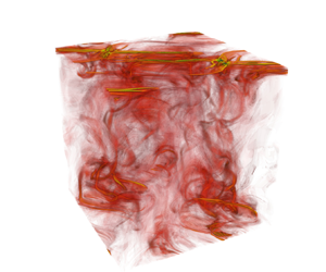
We examine a specific broad-scale Beltrami flow in a horizontally-periodic domain. While the flow is steady in theory, instability is triggered by very-low-level numerical noise. Such instability is generally expected for Euler flows, as none satisfy the Arnol'd conditions for stability (Rouchon Reference Rouchon1991). We find that after a period of time that is long compared to the eddy turnaround time  $4{\rm \pi} /|\boldsymbol {\omega }|_{max}$, where $\boldsymbol {\omega }$ is the vector vorticity at the initial time, the flow breaks down in a way that appears to be independent of numerical resolution. Thereafter, the vorticity magnitude rises sharply and the flow becomes turbulent, developing an energy spectrum having a power-law decay in total wavenumber with slope close to $-5/3$, as theorised by Kolmogorov (Reference Kolmogorov1941) and Onsager (Reference Onsager1945). As the flow decays (here due to horizontal hyperviscous damping), it becomes increasingly anisotropic due to the faster decay of the interior flow relative to the near-boundary flow. The boundaries constrain the bending and twisting of vortex lines, leading to this anisotropy. Notably, we observe intense front formation – near discontinuous variations of the surface velocity field – reminiscent of actual atmospheric flows (see Hoskins Reference Hoskins1974; Hoskins, Neto & Cho Reference Hoskins, Neto and Cho1984; Clark, Parker & Hanley Reference Clark, Parker and Hanley2021) despite the absence of buoyancy or temperature variations in the model studied here.
Beltrami flows occur, for example, in helical flows such as rotating thunderstorms (see Lilly Reference Lilly1986a,Reference Lillyb; Brandes, Davies-Jones & Johnson Reference Brandes, Davies-Jones and Johnson1988, and references therein), but also in magnetohydrodynamics (see Rudraiah Reference Rudraiah1970; Dritschel Reference Dritschel1991; Chen & Yuen Reference Chen and Yuen2021). In the latter, a force-free magnetic field  $\boldsymbol {B}$ satisfies ${\boldsymbol {\nabla }}\times \boldsymbol {B}=\varkappa \boldsymbol {B}$, where the scalar $\varkappa$ may vary in space but is constant along field lines. The analogous hydrodynamical situation is $\boldsymbol {\omega }={\boldsymbol {\nabla }}\times \boldsymbol {u}=\varkappa \boldsymbol {u}$, where $\boldsymbol {u}$ is the velocity field, and $\varkappa$ is constant along streamlines (both situations are considered in Dritschel Reference Dritschel1991). Below, we consider the simplest special case where $\varkappa$ is constant throughout space (Trkal Reference Trkal1919). We also discuss briefly the extension to magnetohydrodynamics.
There is a deep connection between Beltrami flows and the helicity invariant in Euler flows, first discovered by Moreau (Reference Moreau1961) in the hydrodynamical context. This invariant is associated with the ‘knottedness’ of vortex lines (Moffatt Reference Moffatt1969), and has been used to prove the existence of a wide class of Beltrami flows in  ${\mathbb {R}}^3$ (Enciso & Peralta-Salas Reference Enciso and Peralta-Salas2015). Helicity is conserved over any material volume bounded by vortex lines, i.e. vortex tubes, a result that depends only on the form of the vorticity equation (as discussed and extended in Moffatt Reference Moffatt2018).
The numerical study below is conducted in the absence of any external forces and by casting the Euler equations into vorticity form. The horizontally periodic flow is confined vertically between parallel plates with free-slip impermeable boundaries. The only boundary condition that we apply is no normal flow,  $w=0$, where $w$ is the vertical velocity component. Importantly, we do not also impose the stress-free condition $\partial {u}/\partial {z}=\partial {v}/\partial {z}=0$, tantamount to imposing zero horizontal vorticity. The Beltrami flows considered do not satisfy these conditions, and moreover, permitting non-zero horizontal vorticity is necessary in other applications, in particular to density-stratified flows where baroclinic processes generate horizontal vorticity, including on the boundaries, when density (or temperature) is permitted to vary there (Gill Reference Gill1982; Vallis Reference Vallis2006).
A survey of the literature indicates that, without exception, past studies of bounded 3-D flows have imposed both no normal flow and stress-free conditions, even when density variations are included (see e.g. Wen et al. Reference Wen, Goluskin, LeDuc, Chini and Doering2020). Numerically, this is convenient especially for spectral methods, since either a sine or a cosine series in the vertical coordinate  $z$ can be used to satisfy exactly all of the boundary conditions (see below for details). Moreover, such series are compatible with the relation between vorticity and velocity, $\boldsymbol {\omega }={\boldsymbol {\nabla }}\times \boldsymbol {u}$, as well as the isochoric and solenoidal conditions $\boldsymbol {\nabla }\boldsymbol {\cdot }\boldsymbol {u}=0$ and $\boldsymbol {\nabla }\boldsymbol {\cdot }\boldsymbol {\omega }=0$. The general inviscid situation where the horizontal vorticity is allowed to vary on each boundary cannot be treated this simply, as explained in § 3. As far as we are aware, there is no numerical method available that consistently treats this case in 3-D flows. With the exception of the vertical velocity component $w$, one cannot assume Dirichlet or Neumann boundary conditions, nor indeed any boundary conditions.
Lam & Banerjee (Reference Lam and Banerjee1992) investigated the effect of shear near surfaces using no slip and free-slip (including stress-free) boundaries. Their pseudo-spectral method employed Chebyshev polynomials in the direction normal to the surfaces. Similarly, Pan & Banerjee (Reference Pan and Banerjee1995) applied this approach to study turbulence in a channel flow configuration with a free-surface (e.g. an air–water interface). In a study of potential singularity formation starting from anti-parallel vortices, Kerr (Reference Kerr1993) introduced a poloidal-toroidal decomposition of the velocity field and expanded the required functions in Chebyshev polynomials in the coordinate perpendicular to the symmetry plane to enhance resolution. His method, however, exploits symmetry to enforce the free-slip condition on the symmetry plane, by using functions that are either even or odd. This symmetry is not general, and is not characteristic of the Beltrami flow studied here. Instead of Chebyshev polynomials, an alternative is to use staggered grids as introduced by Arakawa & Lamb (Reference Arakawa and Lamb1977). In Shen et al. (Reference Shen, Zhang, Yue and Triantafyllou1999) and Li & Yang (Reference Li and Yang2019), for example, the vertical velocity component  $w$ is shifted by half a cell width from the regular grid points. Staggered grids, however, are inconsistent when the boundaries contain non-zero horizontal vorticity, since the latter involves vertical derivatives of the horizontal velocity, and this is located on the wrong grid. One would ideally like to represent horizontal vorticity on the ‘half’ grid, but this is consistent only when the horizontal vorticity vanishes on the boundaries like vertical velocity. A different approach is required, as argued in § 3. Notably, free-slip and stress-free conditions are commonly used in idealised atmospheric studies, e.g. of squall lines (Fovell & Tan Reference Fovell and Tan2000).
A common expedient used to control the energy cascade and prevent the build up of energy at the grid scale is to add hyperdiffusion to the evolution equations, since this permits one to mostly limit the numerical damping to small scales, compared to ordinary (molecular) diffusion (for a discussion, see Frey, Dritschel & Böing Reference Frey, Dritschel and Böing2022). However, the presence of free-slip boundaries requires additional boundary conditions for consistency (Jones & Roberts Reference Jones and Roberts2005). While these can be enforced readily in the stress-free situation discussed above, they cannot in the Beltrami flow problem that we address in this paper, or in any situation where there is non-zero horizontal vorticity on the boundaries. Invariably, any attempt to apply hyperdiffusion using a compound 3-D Laplace operator magnifies numerical errors near the boundaries, eventually causing the energy to blow up at later times.
To overcome this issue, here we propose a mixed pseudo-spectral approach where prognostic (evolution) variables are decomposed in a mixed spectral form, consisting of a part that vanishes at each boundary (represented as a sine series in  $z$), and two other parts accounting for non-zero boundary values. These other parts are harmonic functions (solutions of Laplace's equation) that vanish on the opposite boundary. These functions arise from a variational problem where one seeks to minimise the squared gradient of a field interpolating between known boundary values over the domain while enforcing boundary values. To avoid the problem with hyperdiffusion discussed above, instead a compound two-dimensional (2-D) Laplace operator is employed. Finally, we use the less aggressive but effective filter of Hou & Li (Reference Hou and Li2007) as a replacement for the ‘ $2/3$’ de-aliasing rule. Such a filter is essential to control aliasing errors that may otherwise lead to code divergence and spurious small-scale features.
The paper is organised as follows. In § 2, we start with the vorticity form of the Euler equations and derive a class of (steady) Beltrami flows confined between two parallel free-slip boundaries. Next, in § 3, we provide a detailed description of the new numerical method developed to be able to study the instability of these Beltrami flows, and indeed any flow with non-zero horizontal vorticity on the boundaries. For such flows, there are no symmetries to exploit and great care is required to avoid spurious numerical artefacts. Our main findings are reported in § 4, where we examine the instability growth, saturation and decay for a wide range of numerical resolutions. The paper concludes with a summary and outlook in § 5.
2. A class of Beltrami flows
2.1. Hydrodynamic Beltrami flows
We consider the incompressible Euler equations in vorticity form, ignoring any body forces,
 $$\begin{gather} \boldsymbol{\omega}_t = {\boldsymbol{\nabla}}\times (\boldsymbol{u}\times\boldsymbol{\omega}), \end{gather}$$
 $$\begin{gather}\boldsymbol{\nabla}\boldsymbol{\cdot}\boldsymbol{u} = 0, \end{gather}$$
where  $\boldsymbol {u}(\boldsymbol {x}, t) = (u, v, w)$ denotes the velocity field, $\boldsymbol {\omega }(\boldsymbol {x}, t) = (\xi, \eta, \zeta )$ denotes the vorticity field, and subscripts $t$,
$t$,  $x$,
$x$,  $y$ and $z$ denote partial differentiation. Furthermore, we have $\boldsymbol {\omega }={\boldsymbol {\nabla }}\times \boldsymbol {u}$, which effectively provides $\boldsymbol {u}$ given $\boldsymbol {\omega }$ (see below). It follows that the vorticity is solenoidal, $\boldsymbol {\nabla }\boldsymbol {\cdot }\boldsymbol {\omega }=0$, and by (2.1) it remains so for all time.
The domain is horizontally periodic (or may be unbounded), and confined between parallel free-slip boundaries at  $z=z_{min}=-L_z/2$ and $z=z_{max}=L_z/2$ without loss of generality. On these boundaries, the vertical velocity must vanish, $w=0$. No other boundary conditions apply. No others are required to recover the velocity field from the vorticity field, as shown below.
We now assume that the flow is of Beltrami type. Such flows are characterised by vorticity being everywhere parallel to velocity, so that  $\boldsymbol {u}\times \boldsymbol {\omega } = \boldsymbol {0}$ and the flow remains steady. In general, we may take
 \begin{equation} \boldsymbol{\omega}(\boldsymbol{x}, t) = \varkappa\,\boldsymbol{u}(\boldsymbol{x}, t) \end{equation}
for some scalar field  $\varkappa$ that is constant on streamlines (curves tangent to $\boldsymbol {u}$). Here, we consider the special case where $\varkappa$ is a non-zero constant (then the flow is known as a Trkalian flow; see Trkal Reference Trkal1919). Using the relation $\boldsymbol {\omega }={\boldsymbol {\nabla }}\times \boldsymbol {u}$, it follows that the flow is determined from the solution to the linear equation ${\boldsymbol {\nabla }}\times \boldsymbol {u}=\varkappa \boldsymbol {u}$, subject to the homogeneous boundary conditions on the vertical velocity $w$.
$w$.
We start by seeking a solution of the form  $\boldsymbol {u}(\boldsymbol {x})=\mathrm {Re}\{\hat {\boldsymbol {u}}(z)\,{\rm e}^{\mathrm {i}\varphi }\}$, where $\mathrm {Re}$ denotes the real part, and $\varphi =kx+ly$ is the horizontal phase, while $k$ and $l$ are arbitrary non-negative wavenumbers (but $k^2+l^2>0$). First, we must ensure incompressibility, $\boldsymbol {\nabla }\boldsymbol {\cdot }\boldsymbol {u}=0$:
 \begin{equation} \mathrm{i} k\hat{u}+\mathrm{i} l\hat{v}+\hat{w}' = 0, \end{equation}
where a prime denotes an ordinary  $z$ derivative. Linearity allows us to strip away the phase dependence ${\rm e}^{\mathrm {i}\varphi }$ and ignore the real part, since $\mathrm {Re}\{\hat {f}\,{\rm e}^{\mathrm {i}\varphi }\}=0$ can be satisfied for all $\varphi$ if and only if $\hat {f}=0$. Next, it is useful to consider the vertical component of ${\boldsymbol {\nabla }}\times \boldsymbol {u}=\varkappa \boldsymbol {u}$, namely $v_x-u_y=\varkappa w$:
 \begin{equation} \mathrm{i} k\hat{v}-\mathrm{i} l\hat{u}=\varkappa\hat{w} . \end{equation}
Combining (2.4) and (2.5), we have
 \begin{equation} \hat{u}=\mathrm{i}\,\frac{k\hat{w}'+l\varkappa\hat{w}}{k^2+l^2}, \quad \hat{v}=\mathrm{i}\,\frac{l\hat{w}'-k\varkappa\hat{w}}{k^2+l^2} . \end{equation}
Now we consider the  $x$ component of ${\boldsymbol {\nabla }}\times \boldsymbol {u}=\varkappa \boldsymbol {u}$, namely $w_y-v_z=\varkappa u$:
 \begin{equation} \mathrm{i} l\hat{w}-\hat{v}'=\varkappa\hat{u} . \end{equation}
Replacing  $\hat {u}$ and $\hat {v}$ by their expressions in (2.6a,b), we find after some simplification a linear, constant-coefficient, second-order equation for $\hat {w}$:
 \begin{equation} \hat{w}''+(\varkappa^2-k^2-l^2)\hat{w}=0 . \end{equation}
The same equation follows from the  $y$ component of ${\boldsymbol {\nabla }}\times \boldsymbol {u}=\varkappa \boldsymbol {u}$.
Let  $m=\sqrt {\varkappa ^2-k^2-l^2}$ denote the vertical wavenumber. Note that $m$ must be real to satisfy the homogeneous boundary conditions at $z=-L_z/2$ and $L_z/2$, and indeed, $m=(2j-1){\rm \pi} /L_z$ for any positive integer $j$. Then the solution is $\hat {w}=A\cos {mz}$ for arbitrary $A$, and the constant is $\varkappa =\pm \sqrt {k^2+l^2+m^2}$.
Taking  $A=1$ without loss of generality, the horizontal velocity amplitudes from (2.6a,b) are
 \begin{equation} \hat{u}={-}\mathrm{i}\,\frac{km\sin{mz}-l\varkappa\cos{mz}}{k^2+l^2}, \quad \hat{v}={-}\mathrm{i}\,\frac{lm\sin{mz}+k\varkappa\cos{mz}}{k^2+l^2}. \end{equation}
Hence, since  $\mathrm {Re}\{-\mathrm {i}\,{\rm e}^{\mathrm {i}\varphi }\}=\sin (kx+ly)$, the Beltrami flow in physical space is
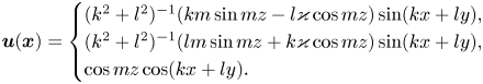 \begin{equation} \boldsymbol{u}(\boldsymbol{x}) = \begin{cases} (k^2+l^2)^{{-}1}(km\sin{mz}-l\varkappa\cos{mz})\sin(kx+ly), \\ (k^2+l^2)^{{-}1}(lm\sin{mz}+k\varkappa\cos{mz})\sin(kx+ly), \\ \cos{mz}\cos(kx+ly) . \end{cases} \end{equation}
The corresponding vorticity is  $\boldsymbol {\omega }=\varkappa \boldsymbol {u}$. Note that any linear superposition of these solutions having the same value of $\varkappa$ is still a steady Beltrami flow.
One can show that  $\|\boldsymbol {\omega }\|_{max}=\varkappa ^2/\sqrt {k^2+l^2}$, and this occurs at locations where both $\cos (kx+ly)=0$ and $\sin {mz}=0$, i.e. along horizontal lines in the planes $z=n{\rm \pi} /m=nL_z/(2j-1)$, for positive integers $j$, and integers $n$ satisfying $|2n|<2j-1$. Note that $m=(2j-1){\rm \pi} /L_z$ has been used, which ensures $w=0$ along $z=\pm L_z/2$.
Note that the solution derived above is similar to the viscous decaying Beltrami flow solution derived by Shapiro (Reference Shapiro1993). An important difference is that the latter applies only to fully periodic boundary conditions (including those in  $z$). The form of the solution also differs as a result. Shapiro (Reference Shapiro1993) points out that Beltrami flows are inconsistent with either no-slip or stress-free boundary conditions. But as we show here, Beltrami flows are consistent with free-slip boundary conditions having non-zero horizontal vorticity (stress).
For a Beltrami flow, the pressure field  $p$ (for unit density $\rho$) satisfies the Bernoulli relation $\boldsymbol {\nabla }(p+\tfrac 12|\boldsymbol {u}|^2)=0$ since $\boldsymbol {u}\times \boldsymbol {\omega }=0$. (This follows from the steady form of the momentum equations after making use of a vector identity.) Without loss of generality, we can take the global mean pressure to be zero in an incompressible flow, leading to the result
 \begin{equation} p = \frac14 \left( \frac{m^2}{k^2+l^2} \cos(2kx+2ly) - \cos(2mz) \right) . \end{equation}
This satisfies  $p_z = 0$ on each boundary, as required. In the incompressible 3-D Euler equations, the pressure is determined from the divergence of the momentum equations, namely
 \begin{equation} \nabla^2 p ={-}\boldsymbol{\nabla}\boldsymbol{\cdot}((\boldsymbol{u}\boldsymbol{\cdot}\boldsymbol{\nabla})\boldsymbol{u}) = 2(J_{xy}(u,v)+J_{yz}(v,w)+J_{zx}(w,u)) , \end{equation}
where  $J_{ab}(f,g)\equiv f_a g_b - f_b g_a$ is the Jacobian. This leads to the same result for $p$ in (2.11) when the Beltrami flow solution in (2.10) is used.
Finally, the domain-average kinetic energy  $\mathcal {K}$ of the Beltrami flow (2.10) is
 \begin{equation} \mathcal{K} = \frac{1}{4} \left(1 + \frac{m^2}{k^2+l^2}\right). \end{equation}
The domain-average enstrophy (the mean-square vorticity divided by 2) is  $\mathcal {\varUpsilon }=\varkappa ^2\mathcal {K}$. Only energy $\mathcal {K}$ and helicity $\mathcal {H}$ (see below) are conserved by the time-dependent Euler equations. Below, we monitor $\mathcal {K}$, $\mathcal {H}$ and $\mathcal {\varUpsilon }$ in numerical simulations starting from a specific (weakly perturbed) Beltrami flow.
2.2. Magnetohydrodynamic Beltrami flows
The equations governing inviscid, incompressible magnetohydrodynamics (see e.g. Chandrasekhar Reference Chandrasekhar1981; Dritschel Reference Dritschel1991; Tobias Reference Tobias2021) in vorticity form are
 $$\begin{gather} \boldsymbol{\omega}_t = {\boldsymbol{\nabla}}\times(\boldsymbol{u}\times\boldsymbol{\omega} + \boldsymbol{j}\times\boldsymbol{B}), \end{gather}$$
 $$\begin{gather}\boldsymbol{B}_t = {\boldsymbol{\nabla}}\times(\boldsymbol{u}\times\boldsymbol{B}) + \nu_{B}\,\nabla^2\boldsymbol{B}, \end{gather}$$
where the new symbols are the magnetic field  $\boldsymbol {B}$, the current density $\boldsymbol {j}={\boldsymbol {\nabla }}\times \boldsymbol {B}$, and the magnetic diffusivity $\nu _B$. Here, $\boldsymbol {B}$ has been scaled by $\sqrt {\rho \mu }$, where $\rho$ is the (constant) fluid density, and $\mu$ is the magnetic permeability, so that $\boldsymbol {B}$ has units of velocity. Similarly, $\boldsymbol {j}$ has been scaled by $\sqrt {\rho /\mu }$, so that $\boldsymbol {j}={\boldsymbol {\nabla }}\times \boldsymbol {B}$ is analogous to $\boldsymbol {\omega }={\boldsymbol {\nabla }}\times \boldsymbol {u}$. Furthermore, we have the solenoidal constraint $\boldsymbol {\nabla }\boldsymbol {\cdot }\boldsymbol {B}=0$ as well as $\boldsymbol {\nabla }\boldsymbol {\cdot }\boldsymbol {j}=0$, which follows from the definition of $\boldsymbol {j}$.
Following Dritschel (Reference Dritschel1991), a class of Beltrami flows may be constructed assuming  $\boldsymbol {\omega }=\varkappa \boldsymbol {u}$ as before, but additionally $\boldsymbol {B}=c\boldsymbol {u}$, where $c$ is spatially uniform but depends on time when $\nu _B>0$. By taking the curl of $\boldsymbol {B}=c\boldsymbol {u}$, it follows that $\boldsymbol {j}=c\boldsymbol {\omega }$. Moreover, using $\boldsymbol {\omega }=\varkappa \boldsymbol {u}$, we have $\boldsymbol {j}=c\varkappa \boldsymbol {u}$. But $\boldsymbol {B}=c\boldsymbol {u}$ then implies that all nonlinear terms in (2.14) and (2.15) vanish. In particular, $\boldsymbol {\omega }_t=\boldsymbol{0}$, so the flow is steady – and is precisely the same as derived above for the purely hydrodynamic case.
In the induction equation (2.15), note that  $\nabla ^2\boldsymbol {B}=-{\boldsymbol {\nabla }}\times ({\boldsymbol {\nabla }}\times \boldsymbol {B})=-{\boldsymbol {\nabla }}\times \boldsymbol {j}=$ $-c\varkappa \,{\boldsymbol {\nabla }}\times \boldsymbol {u}=-c\varkappa ^2\boldsymbol {u}$. But the left-hand side of (2.15) reduces to $(\mathrm {d} c/\mathrm {d} t)\boldsymbol {u}$ since $\boldsymbol {u}$ is time-independent. Hence, equating both sides, we conclude
 \begin{equation} \frac{\mathrm{d} c}{\mathrm{d} t}={-}\nu_B\varkappa^2 c, \end{equation}
which gives the exponentially decaying solution  $c(t)=c(0)\exp (-\nu _B\varkappa ^2 t)$.
Notably, the vertical magnetic field, proportional to the vertical velocity, vanishes at each boundary, consistent with perfectly conducting boundaries. There is no boundary condition on the horizontal magnetic field; magnetic diffusivity does not constrain the field to be zero (unlike molecular diffusion acting on velocity).
In conclusion, there is an analogous class of Beltrami solutions when a magnetic field is present, only the field decays exponentially in time. Investigating the stability of these solutions is left to future work.
3. Numerical method
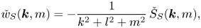
We consider a vertically confined flow between two parallel free-slip boundaries, on which we allow non-zero stress (equivalently, non-zero horizontal vorticity). This is the general situation that applies in an inviscid flow, and in particular applies in a density-stratified flow where baroclinic production of vorticity may occur throughout the flow, including on the boundaries. While we ignore density variations, in order to study the stability of Beltrami flows, we must allow for stress on the boundaries.
The presence of boundary stress, however, makes a standard pseudo-spectral numerical method infeasible. We have found that this method, employing standard 3-D hyperdiffusion, leads to unphysical results that exhibit an energy increase after the occurrence of the instability. The source of this energy increase is the vertical hyperdiffusion, which enhances near-boundary errors that become dominant as the large-scale structures cascade and decay into small-scale structures. Another problem with the pseudo-spectral method is that nearly all fields must be expanded as cosine series in  $z-z_{min}$ to allow for non-zero boundary values; only the vertical velocity $w$ has zero boundary values and is naturally expanded as a sine series. As a result, the inversion of vorticity to find the velocity is not straightforward. From the forms of the vorticity components, namely
 \begin{equation} \xi=w_y-v_z, \quad \eta=u_z-w_x, \quad \zeta=v_x-u_y, \end{equation}
one can see readily that if  $u$ and $v$ are expressed as cosine series in $z-z_{min}$, then this implies that $\xi$ and $\eta$ should be expressed as sine series – i.e. have zero boundary values. This is the stress-free situation, but not one that we can exploit in this work, or in general. Instead, we develop a special vorticity inversion method, which makes use of a field decomposition (described next) that permits arbitrary boundary values for all fields except for vertical velocity.
3.1. Field decomposition
The proposed field decomposition consists of two steps. First, a scalar field  $q(\boldsymbol {x})$ in physical space (suppressing time $t$) is transformed into semi-spectral space $\hat {q}(\boldsymbol {k}, z)\equiv \hat {q}(k, l, z)$ with horizontal wavenumbers $k$ and $l$, and separated into a harmonic part $\hat {q}_{H}(\boldsymbol {k}, z)$, and a vertical sine series part $\hat {q}_{S}(\boldsymbol {k}, z)$, where
 $$\begin{gather} \hat{q}_H(\boldsymbol{k}, z) = \hat{q}_{-}(\boldsymbol{k})\,\varphi_{-}(\boldsymbol{k}, z) + \hat{q}_{+}(\boldsymbol{k})\,\varphi_{+}(\boldsymbol{k}, z), \end{gather}$$
 $$\begin{gather}\hat{q}_S(\boldsymbol{k}, z) = \sum_{j = 1}^{n_z-1}\check{q}(\boldsymbol{k},m)\sin m(z-z_{min}) , \end{gather}$$
with  $m = {\rm \pi}j / L_z$. Note that here the wavenumbers $k$,
$k$,  $l$ and $m$ take all permissible values, unlike for the base Beltrami flow in § 2. The quantities $\hat {q}_{-}(\boldsymbol {k})=\hat {q}(\boldsymbol {k},z_{min})$ and $\hat {q}_{+}(\boldsymbol {k})=\hat {q}(\boldsymbol {k},z_{max})$ are the boundary values of $\hat {q}(\boldsymbol {k}, z)$, while the fixed functions $\varphi _{\pm }$ are defined below. The harmonic part in physical space satisfies Laplace's equation, i.e. $\nabla ^2 q_H = 0$. (The use of harmonic functions is justified below.) Equation (3.3) makes use of a fast Fourier transform to compute the coefficients $\check {q}(\boldsymbol {k},m)$ in full (3-D) spectral space. In the remainder of this paper, we refer to fields in this form as mixed spectral fields, and label such a field with an overscript as $\mathring {q}$.
The harmonic functions  $\varphi _{\pm }$ are given by
 \begin{equation} \varphi_{-}(\boldsymbol{k}, z) = \frac{\sinh k_h(z_{max} - z)}{\sinh{k_h L}} \quad\text{and}\quad \varphi_{+}(\boldsymbol{k}, z) = \frac{\sinh k_h(z - z_{min})}{\sinh{k_h L}}, \end{equation}
where  $k_h^2 = k^2 + l^2$. They are solutions to Laplace's equation in semi-spectral space,
 \begin{equation} \varphi_{{\pm}}'' - k_h^2\varphi_{{\pm}} = 0, \end{equation}
such that  $\varphi _{-}(\boldsymbol {k}, z_{min}) = \varphi _{+}(\boldsymbol {k}, z_{max}) = 1$ and $\varphi _{-}(\boldsymbol {k}, z_{max}) = \varphi _{+}(\boldsymbol {k}, z_{min}) = 0$. Any field in mixed spectral space can therefore be stored efficiently (cf. figure 1) in a single 3-D array for computation. The arrays $\varphi _{\pm }$ are pre-computed and stored during initialisation.
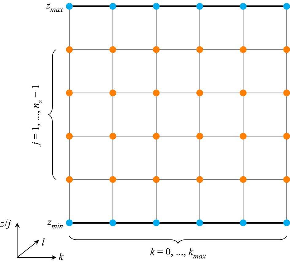
Figure 1. Field representation in mixed spectral space. The  $l$ direction is not shown explicitly. The $kl$-planes at the free-slip boundaries $z=z_{min}$ and $z_{max}$, highlighted by the thick black lines, are in semi-spectral space; otherwise, a field is in full spectral space (obtained by a sine transform in $z$).
$z$).
The decomposition using harmonic functions is motivated by the following variational problem. Find the field  $q_H(\boldsymbol {x})$ that has the minimum domain integral of $|\boldsymbol {\nabla } q_H|^2$ and which matches prescribed boundary values $q_H(x,y,z_{min})=q_{-}(x,y)$ and $q_H(x,y,z_{max})=q_{+}(x,y)$. Arguably, this is the smoothest field $q_H(\boldsymbol {x})$ that interpolates between the boundary values. The solution to this problem results in Laplace's equation $\nabla ^2 q_H=0$, subject to prescribed boundary conditions. This is the solution used above in semi-spectral space in (3.2). Note that $q_S=q-q_H$ is the difference between the full field $q$ and the harmonic part $q_H$ interpolating between the boundary values. Thus $q_S=0$ on the boundaries. Importantly, $q_S$ is not the interior part of the field $q$.
$q$.
3.2. Vorticity inversion
The evolution of vorticity in (2.1) requires the calculation of the velocity from the vorticity, a process called ‘inversion’. Using  $\boldsymbol {\nabla }\boldsymbol {\cdot }\boldsymbol {u}=u_x+v_y+w_z=0$ and (3.1a–c), it follows that $\xi _y-\eta _x=\nabla ^2 w$, providing a Poisson equation for the vertical velocity $w$. In semi-spectral space, this is
 \begin{equation} \hat{w}''(\boldsymbol{k}, z) - k_h^2\,\hat{w}(\boldsymbol{k}, z) = \hat{S}(\boldsymbol{k}, z), \end{equation}
subject to  $\hat {w}(\boldsymbol {k}, z_{min}) = \hat {w}(\boldsymbol {k}, z_{max}) = 0$. Note that the source $\hat {S}=\mathrm {i} l\hat {\xi }-\mathrm {i} k\hat {\eta }$ may be non-zero in general on the boundaries (although it happens to be zero for the exact Beltrami flow). The solution $\hat {w}$ is found in decomposed form
 \begin{equation} \hat{w}''_{H} - k_h^2\hat{w}_{H} = \hat{S}_H \quad\text{and}\quad \hat{w}''_{S} - k_h^2\hat{w}_{S} = \hat{S}_S, \end{equation}
where the solution of the sine series part  $\hat {w}_{S}$ is obtained in full spectral space by multiplication of the source term with the Green's function,
 \begin{equation} \check{w}_{S}(\boldsymbol{k}, m) ={-}\frac{1}{k^2 + l^2 + m^2}\,\check{S}_{S}(\boldsymbol{k}, m), \end{equation}
for all  $m > 0$ (recall that $m = {\rm \pi}j / L_z$ for positive integers $j$). The solution of the harmonic part $\hat {w}_{H}$ is performed analytically, and it can be verified that
 \begin{equation} \hat{w}_{H}(\boldsymbol{k}, z) = \hat{S}_{-}(\boldsymbol{k})\,\theta_{-}(\boldsymbol{k}, z) + \hat{S}_{+}(\boldsymbol{k})\,\theta_{+}(\boldsymbol{k}, z), \end{equation}
where
 $$\begin{gather} \theta_{-}(\boldsymbol{k}, z) = \frac{\sinh{k_h L}}{2k_h} [(z_{max}-z)\,\varphi_{+}(\boldsymbol{k}, z) - (z-z_{min})\,\varphi_{-}(\boldsymbol{k}, z)\cosh{k_h L}], \end{gather}$$
 $$\begin{gather}\theta_{+}(\boldsymbol{k}, z) = \frac{\sinh{k_h L}}{2k_h} [(z-z_{min})\,\varphi_{-}(\boldsymbol{k}, z) - (z_{max}-z)\,\varphi_{+}(\boldsymbol{k}, z)\cosh{k_h L}]. \end{gather}$$
Note that the functions  $\theta _{\pm }$ vanish on both boundaries.
The horizontal velocity components  $u$ and $v$ are found by combining the relations $v_x-u_y=\zeta$ for vertical vorticity and $u_x+v_y=-w_z$ for incompressibility. In semi-spectral space, this yields
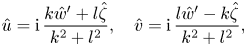 \begin{equation} \hat{u}=\mathrm{i}\,\frac{k\hat{w}'+l\hat{\zeta}}{k^2+l^2}, \quad \hat{v}=\mathrm{i}\,\frac{l\hat{w}'-k\hat{\zeta}}{k^2+l^2}, \end{equation}
for  $k^2+l^2>0$. No further boundary conditions are required. The $z$ derivative $\hat {w}'$ is calculated analytically using wavenumber multiplication of $\check {w}_{S}$ and a cosine transform, and by differentiating the boundary contribution $\hat {w}_{H}$ (using pre-stored arrays for $\theta '_{\pm }$, details omitted).
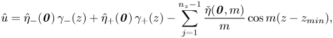
The horizontally uniform flow for  $k=l=0$ is instead found directly from the definitions of the horizontal vorticity components, which reduce to $\hat {\xi }=-\hat {v}_z$ and $\hat {\eta }=\hat {u}_z$ in this case. Then $\hat {u}$ and $\hat {v}$ are found directly by integrating $\hat {\eta }$ and $-\hat {\xi }$, requiring that the domain-mean values of $\hat {u}$ and $\hat {v}$ vanish without loss of generality. From (3.2) and (3.3), it follows that
 \begin{equation}
\hat{u}=\hat{\eta}_{-}(\boldsymbol{0})\,\gamma_{-}(z) +
\hat{\eta}_{+}(\boldsymbol{0})\,\gamma_{+}(z) - \sum_{j =
1}^{n_z-1}\frac{\check{\eta}(\boldsymbol{0},m)}{m}\cos
m(z-z_{min}), \end{equation}
\begin{equation}
\hat{u}=\hat{\eta}_{-}(\boldsymbol{0})\,\gamma_{-}(z) +
\hat{\eta}_{+}(\boldsymbol{0})\,\gamma_{+}(z) - \sum_{j =
1}^{n_z-1}\frac{\check{\eta}(\boldsymbol{0},m)}{m}\cos
m(z-z_{min}), \end{equation}
where  $m={\rm \pi} j/L_z$ as before, and
 \begin{equation} \gamma_{-}(z)=\frac{L_z^2-3(z_{max}-z)^2}{6L_z}, \quad \gamma_{+}(z)=\frac{3(z-z_{min})^2-L_z^2}{6L_z}. \end{equation}
The analogous expression for  $\hat {v}$ is found by replacing $\eta$ by $-\xi$ in (3.13).
3.3. Vorticity tendency calculation
As noted in § 2, for a Beltrami flow, the right-hand side of (2.1) vanishes, so the vorticity remains steady. However, numerical errors lead to vorticity evolution as  $\boldsymbol {u}$ loses alignment with $\boldsymbol {\omega }$. Eventually, this evolution leads to instability – a physical instability that, however, is triggered by numerical noise, as documented in the next section. Here, we discuss the numerical method used to update the vorticity field in a general unsteady flow.
In (2.1), we first compute the vector  $\boldsymbol {u}\times \boldsymbol {\omega }=(P,Q,R)$, then compute the components of the vorticity tendency from
 \begin{equation} \xi_t = R_y - Q_z, \quad \eta_t = P_z - R_x, \quad \zeta_t = Q_x - P_y, \end{equation}
where
 \begin{equation} P = v\zeta - w\eta, \quad Q = w\xi - u\zeta, \quad R = u\eta - v\xi. \end{equation}
All  $z$ derivatives, which occur only in $\xi _t$ and $\eta _t$, are computed in semi-spectral space on the $z$ grid by centred differences, with linear extrapolation at each boundary. All $x$ and $y$ derivatives are computed spectrally by wavenumber multiplication in mixed spectral space. To maintain $\boldsymbol {\nabla }\boldsymbol {\cdot }\boldsymbol {\omega }=0$ at all times, a solenoidal correction is applied to vorticity at each time step (see below).
3.4. Dissipation operator
Three-dimensional flows generically exhibit a strong cascade of energy from large to small scales, particularly as they become turbulent. This cascade cannot be resolved indefinitely at any finite resolution, and the key task is to remove energy arriving at the smallest scale without seriously affecting the larger resolved scales. Ordinary molecular diffusion does this physically (as long as the Kolmogorov length  $L_K$ is well resolved, see below), but such diffusion damps an extensive range of scales and is not relevant when modelling ultra-high Reynolds number flows widely occurring in geophysical and astrophysical flows. Instead, researchers have often used hyperdiffusion, a dissipation operator ${\mathcal {D}}\propto \nabla ^{2{\mathsf{p}}}$ for integers ${\mathsf{p}}>1$, to focus dissipation primarily at the smallest scales. The expectation is that hyperdiffusion allows a greater range of active scales with much less damping. Hyperdiffusion is, however, not benign, and has some undesirable features such as non-monotonicity, particularly for high-order forms with ${\mathsf{p}}\gg 1$ (for further discussion, see Frey et al. Reference Frey, Dritschel and Böing2022, and references therein).
Here, we use a moderate order,  ${\mathsf{p}}=3$, which helps to reduce the unrealistic amplification of energy at small scales (high wavenumbers) when ${\mathsf{p}}\gg 1$. However, with boundary stress (non-zero horizontal vorticity), the use of the 3-D Laplacian in the hyperdiffusion operator ${\mathcal {D}}$ leads to an unphysical energy growth at late times, after the flow destabilises and breaks down into small-scale turbulence. The problem stems from the $z$ derivative terms in ${\mathcal {D}}$, as demonstrated explicitly in a test example in Appendix B, where we show that hyperdiffusion strongly magnifies numerical errors near the boundaries, eventually leading to energy growth. Mathematically, the use of such hyperdiffusion imposes extra boundary conditions that we cannot justify (Jones & Roberts Reference Jones and Roberts2005). On the other hand, no-stress boundary conditions (which are not applicable here) avoid the problem with hyperdiffusion, as then all fields have either zero odd derivatives or zero even derivatives, and the extra boundary conditions are satisfied automatically.
To avoid this problem when boundary stress is present, we apply only 2-D hyperdiffusion, using the compounded horizontal Laplacian operator. In mixed spectral space, we damp vorticity by subtracting  $\mathring {\mathcal {D}}\circ \mathring {\boldsymbol {\omega }}$ (‘ $\mathring {\mathcal {D}}$ operating on $\mathring {\boldsymbol {\omega }}$’, here simply by multiplication) from the right-hand side of (2.1), where
 \begin{equation} \mathring{\mathcal{D}}(\boldsymbol{k},t) = C\,\omega_{{char}}(t)\,(k_m^2\mathcal{K}(0)/\mathcal{\varUpsilon}(0))^{1/3}(k_h/k_m)^{2{\mathsf{p}}}, \end{equation}
in which  $\omega _{{char}}(t)$ is a characteristic vorticity (see below), $k_m=\max (k_{max},l_{max})$ is the maximum $x$ or $y$ wavenumber (often equal), $k_h=|\boldsymbol {k}|=\sqrt {k^2+l^2}$ as before, $\mathcal {K}(0)$ and $\mathcal {\varUpsilon }(0)$ are the initial (domain-averaged) kinetic energy and enstrophy,
 \begin{equation} \mathcal{K}(t) = \tfrac{1}{2} \langle |\boldsymbol{u}|^2 \rangle \quad \text{and} \quad \mathcal{\varUpsilon}(t) = \tfrac{1}{2} \langle |\boldsymbol{\omega}|^2 \rangle, \end{equation}
and  $C$ is a dimensionless constant, assumed independent of numerical resolution. (Here and below, $\langle q \rangle$ denotes the domain average of a quantity $q$.) The specific form of $\mathring {\mathcal {D}}$ in (3.17) is motivated by the need to resolve the Kolmogorov length $L_K$ at all resolutions. This length is defined via
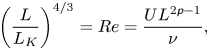 \begin{equation} \left(\frac{L}{L_K}\right)^{4/3} = {Re} = \frac{U L^{2{\mathsf{p}}-1}}{\nu}, \end{equation}
where  $L$ is a characteristic scale of the flow, ${{Re}}$ is the Reynolds number, $U$ is a characteristic velocity, ${\mathsf{p}}$ is the hyperdiffusion order, and $\nu$ is the hyperviscosity coefficient. Here, we have adapted the relationship that applies for standard molecular diffusion, ${\mathsf{p}}=1$ (see e.g. Davidson Reference Davidson2015). To arrive at the form of $\mathring {\mathcal {D}}$ in (3.17), we assume (1) $U\sim \omega _{{char}}(t)\,L$, (2) $L_K\sim k_m^{-1}$, and (3) $L\sim \sqrt {\mathcal {K}(0)/\mathcal {\varUpsilon }(0)}$. This gives
 \begin{equation} \nu \sim \omega_{{char}}(t)\,(k_m^2\,\mathcal{K}(0)/\mathcal{\varUpsilon}(0))^{1/3}k_m^{{-}2{\mathsf{p}}} . \end{equation}
Then, since  $\mathring {\mathcal {D}}=\nu k_h^{2{\mathsf{p}}}$, we recover (3.17) after including a dimensionless pre-factor $C$ in $\nu$ above.
The characteristic vorticity  $\omega _{{char}}(t)$ is computed as in Frey et al. (Reference Frey, Dritschel and Böing2022) but for 3-D flows. The time dependence allows the damping to adjust to the flow dynamically, rather than excessively damp in periods where there is little activity. We first compute the root-mean-square (r.m.s.) vorticity $\omega _{rms}(t)=\sqrt {2\,\mathcal {\varUpsilon }(t)}$. Then, for all grid points where $|\boldsymbol {\omega }|>\omega _{rms}$, we accumulate the sums of $|\boldsymbol {\omega }|$ and $|\boldsymbol {\omega }|^2$, which we call $\omega _{L1}$ and $\omega _{L2}$, respectively. Finally, $\omega _{{char}}=\omega _{L2}/\omega _{L1}$. As argued in Frey et al. (Reference Frey, Dritschel and Böing2022), this measure of a characteristic vorticity is designed to handle situations where intense vorticity is distributed sparsely in the domain, a common situation in a turbulent flow.
3.5. Filtering
Aliasing errors in pseudo-spectral methods are usually reduced with filters (see Goodman, Hou & Tadmor Reference Goodman, Hou and Tadmor1994). Common filters are the ‘ $2/3$ rule’ and the Hou & Li (Reference Hou and Li2007) filter. Although filtering introduces an error near the free-slip boundaries like vertical hyperdiffusion (cf. Appendix B), its effect is weaker and does not cause an energy blow-up, or even an increase. Since the prognostic variables $\mathring {\xi }$, $\mathring {\eta }$ and $\mathring {\zeta }$ are in mixed spectral space, we apply the Hou & Li (Reference Hou and Li2007) filter in two dimensions at $z_{min}$ and $z_{max}$,
 \begin{equation} \hat{\mathcal{F}}(\boldsymbol{k}, z_{min}) = \hat{\mathcal{F}}(\boldsymbol{k}, z_{max}) = \exp\{{-}36[(k/k_{max})^{36} + (l/l_{max})^{36}]\} , \end{equation}
and in three dimensions on the sine series part in the interior,
 \begin{equation} \check{\mathcal{F}}(\boldsymbol{k}, m) = \exp\{{-}36[(k/k_{max})^{36} + (l/l_{max})^{36} + (m/m_{max})^{36}]\}. \end{equation}
In the following, we denote the filtering of a field  $\mathring {q}$ in mixed spectral space by $\mathring {\mathcal {F}}\circ \mathring {q}$, where $\mathring {\mathcal {F}} \equiv \{\hat {\mathcal {F}}, \check {\mathcal {F}}\}$ denotes the complete filter.
3.6. Time stepping
The advection of vorticity from time  $t^n\equiv n\,\Delta t$ to $t^{n+1}$, $n\ge 0$, is performed with the implicit Crank–Nicolson method (or iterative trapezoidal method; see Crank & Nicolson Reference Crank and Nicolson1947) in mixed spectral space,
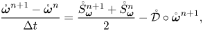 \begin{equation} \frac{\mathring{\boldsymbol{\omega}}^{n+1} - \mathring{\boldsymbol{\omega}}^{n}}{\Delta t} = \frac{\mathring{S}_{\boldsymbol{\omega}}^{n+1} + \mathring{S}_{\boldsymbol{\omega}}^{n}}{2} - \mathring{\mathcal{D}}\circ\mathring{\boldsymbol{\omega}}^{n+1}, \end{equation}
except that the diffusion term is evaluated at  $t^{n+1}$ for greater numerical stability. The first iteration uses $\mathring {S}_{\boldsymbol {\omega }}^{n+1}=\mathring {S}_{\boldsymbol {\omega }}^{n}$ since at this stage we do not yet have an estimate for the fields at $t^{n+1}$. Each iteration provides an improved estimate for $\mathring {\boldsymbol {\omega }}^{n+1}$ and hence $\mathring {S}_{\boldsymbol {\omega }}^{n+1}$ after inverting to find ${\boldsymbol {u}}^{n+1}$; see § 3.2 and (3.16a–c). Explicitly, we update the vorticity using
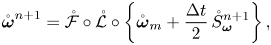 \begin{equation} \mathring{\boldsymbol{\omega}}^{n+1} = \mathring{\mathcal{F}}\circ \mathring{\mathcal{L}}\circ\left\{\mathring{\boldsymbol{\omega}}_m + \frac{\Delta t}{2}\,\mathring{S}_{\boldsymbol{\omega}}^{n+1}\right\}, \end{equation}
where  $\mathring {\mathcal {L}} \equiv 2/(1 + \Delta t\,\mathring {\mathcal {D}})$ and $\mathring {\boldsymbol {\omega }}_m \equiv \mathring {\boldsymbol {\omega }}^{n} + \frac {1}{2}\,\Delta t\,\mathring {S}_{\boldsymbol {\omega }}^{n}$ is fixed during the iteration. Here, we additionally apply the filter operator $\mathring {\mathcal {F}}$ to the updated vorticity. We iterate this equation three times in practice, analogous to a predictor-corrector scheme.
Evolving all three components of the vorticity is redundant on account of the solenoidal condition  $\boldsymbol {\nabla }\boldsymbol {\cdot }\boldsymbol {\omega }=0$. This condition cannot be maintained exactly due to the finite differences carried out in $z$ and the use of the filter $\mathring {\mathcal {F}}$ above. We therefore correct the vorticity immediately before calculating the velocity, in a way closely analogous to how we calculate the horizontal velocity. Specifically, we first compute $\delta \equiv \boldsymbol {\nabla }\boldsymbol {\cdot }\boldsymbol {\omega }$ in semi-spectral space as $\hat {\delta }$. (This requires taking a $z$ derivative of $\hat {\zeta }$ by centred differences, using linear extrapolation of $\hat {\zeta }$ at the boundaries as elsewhere in the numerical code, for consistency.) Next, we seek corrections to the horizontal components $\hat {\xi }$ and $\hat {\eta }$ only, of the form $\hat {\xi }\to \hat {\xi }+\mathrm {i} k\hat {\psi }$ and $\hat {\eta }\to \hat {\eta }+\mathrm {i} l\hat {\psi }$ (effectively adding the horizontal gradient of a potential $\psi$). Requiring that the corrected vorticity satisfy $\boldsymbol {\nabla }\boldsymbol {\cdot }\boldsymbol {\omega }=0$ then implies $\hat {\psi }=k_h^{-2}\hat {\delta }$, from which one obtains the corrected horizontal vorticity components.
In an inviscid fluid with free-slip boundaries, there can be no net flux of vorticity through the boundaries (see Morton Reference Morton1984; Terrington, Hourigan & Thompson Reference Terrington, Hourigan and Thompson2020, Reference Terrington, Hourigan and Thompson2021, Reference Terrington, Hourigan and Thompson2022, and references therein), implying that the domain-mean vorticity  $\langle \boldsymbol {\omega }\rangle$ must remain constant. In fact, the mean vertical vorticity $\zeta =v_x-u_y$ is zero due to horizontal periodicity. Only the horizontal components $\xi =w_y-v_z$ and $\eta =u_z-w_x$ may have a non-zero mean, e.g. due to the presence of a mean shear. In the numerical simulations discussed in the next section, $\langle \boldsymbol {\omega }\rangle$ remains approximately zero when no correction is made, but when the flow becomes turbulent and decays, the mean horizontal vorticity drifts away from zero. To counteract this, we compute and correct the mean horizontal vorticity every time it is updated in (3.24) above (this can be done efficiently in mixed spectral space).
4. Results
4.1. Initial conditions
We focus on a broad-scale Beltrami flow with  $k=l=2$ and $m=1$ (see (2.10)) in the cubic domain $[-{\rm \pi} /2, {\rm \pi}/2]^3$. Then $\varkappa =\pm 3$; here, we choose the positive sign.
The (initial) velocity field is given by
 \begin{equation}
\boldsymbol{u}(\boldsymbol{x},0) = \begin{cases}
\tfrac14(\sin{z}-3\cos{z})\sin(2x+2y), \\
\tfrac14(\sin{z}+3\cos{z})\sin(2x+2y), \\
\cos{z}\cos(2x+2y) , \end{cases}
\end{equation}
\begin{equation}
\boldsymbol{u}(\boldsymbol{x},0) = \begin{cases}
\tfrac14(\sin{z}-3\cos{z})\sin(2x+2y), \\
\tfrac14(\sin{z}+3\cos{z})\sin(2x+2y), \\
\cos{z}\cos(2x+2y) , \end{cases}
\end{equation}
and the corresponding (initial) vorticity is  $\boldsymbol {\omega }=3\boldsymbol {u}$, shown in figure 2. Moreover, $\|\boldsymbol {\omega }\|_{max}=9/\sqrt {8}\approx 3.18198$, which corresponds to a characteristic ‘eddy turnaround time’ $T=4{\rm \pi} /\|\boldsymbol {\omega }\|_{max}\approx 3.94923$. The (domain-mean) kinetic energy is $\mathcal {K}=9/32=0.28125$ in (2.13), while the enstrophy is $\mathcal {\varUpsilon }=\varkappa ^2\mathcal {K}=81/32=2.53125$, implying $|\boldsymbol {\omega }|_{rms}=9/4=2.25$.
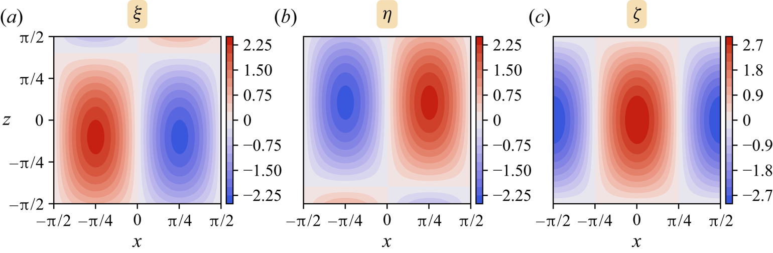
Figure 2. Contour plots (20 iso-levels) of the initial vorticity components  $\boldsymbol {\omega } = (\xi, \eta, \zeta )$ in the $xz$-plane at $y = 0$.
4.2. Choice of hyperviscosity coefficient
An important consideration in simulating the evolution of fluid flows is the appropriate choice of numerical damping. To avoid an unphysical energy growth or even divergence, sufficient damping must be used to absorb the energy cascade arriving at the smallest scales. Here, we justify our choice of damping by varying the hyperdiffusion pre-factor  $C$ in (3.17).
To this end, we conducted a series of  $32^3$ grid-cell simulations of the initial flow specified in (4.1), with $C$ ranging from 10 to 100, in increments of 10. In figure 3, we show the kinetic energy $\mathcal {K}$ and enstrophy $\mathcal {\varUpsilon }$ for a subset of these runs (below, we discuss helicity $\mathcal {H}$ separately). Characteristically, there is an initial period extending to approximately $t=58$ where both quantities remain nearly constant; thereafter, $\mathcal {K}$ decreases while $\mathcal {\varUpsilon }$ grows rapidly over a short period – this is a manifestation of the flow instability, described in detail below. At later times, both $\mathcal {K}$ and $\mathcal {\varUpsilon }$ decay.

Figure 3. Time evolution of the normalised kinetic energy and enstrophy for hyperdiffusion pre-factors  $C = 10, 20, 30, 60,100$.
The lowest damping rates with  $C=10$ and $20$ stand out with a premature decay of kinetic energy and an erratic evolution of enstrophy (taking $C<2$ leads to non-monotonic energy variation for the $32^3$ simulation, not shown). The remaining damping values exhibit closely comparable kinetic energy and enstrophy evolution, but the higher damping values $60$ and $100$ lead to a more rapid decay of enstrophy, as well as a more noticeable decay of kinetic energy before the flow breaks down into turbulence. Based on these results, we have taken $C=30$ to be the default hyperdiffusion pre-factor.
We have verified that  $C=30$ works well at all higher resolutions up to $256^3$, the maximum that we have been able to compute, as demonstrated in figure 4. In all cases, $\mathcal {K}$ begins to decay around the same time and is accompanied by a sharp growth in $\mathcal {\varUpsilon }$. The time of peak enstrophy occurs progressively earlier with increasing resolution, apart from $32^3$, which appears to be too coarse to resolve the instability and its breakdown into turbulence. The peak value of enstrophy grows with resolution, approximately as $n_z^{1.4}$ as shown in figure 4(b), though the sample size is too small to be confident of this scaling. The maximum vorticity magnitude, however, appears to scale similarly.

Figure 4. (a) Time evolutions of the normalised kinetic energy and enstrophy for different grid resolutions (only times 50–100 are shown). The hyperdiffusion pre-factor is  $C=30$ in these and all subsequent results. (b) Peak values (over all time) of enstrophy $\mathcal {\varUpsilon }$ and maximum vorticity magnitude $|\boldsymbol {\omega }|_{max}$ for different grid resolutions. The power-law fit is made using only the three highest resolutions.
4.3. Onset of the instability
We now focus on the highest resolution simulation using  $256^3$ grid cells. The results are qualitatively similar to those obtained at lower resolution, but flow features are much more clearly expressed.
We begin by describing the early stages of the instability development. The justification for calling it an ‘instability’ is that the field differences, e.g.  $\boldsymbol {u}(\boldsymbol {x},t)-\boldsymbol {u}(\boldsymbol {x},0)$, when normalised say to unity in magnitude, are nearly independent of $t$ before the flow breaks down into turbulence. We call this normalised difference the ‘eigenmode’, with the expectation that the same structure would be found from a linear analysis of the equations. (Unfortunately, such an analysis appears to be exceedingly difficult since the basic flow depends on $x+y$ and $z$.)
$z$.)
The eigenmode structure is shown in figure 5 for a  $y=0$ cross-section, and in figure 6 for a $z=0$ cross-section. First, the velocity difference is not proportional to the vorticity difference, so the flow perturbation is not Beltrami, as required to be unsteady. Second, the eigenmode structure is of smaller scale than the original flow. For example, in the $y=0$ cross-section, a fivefold spiral pattern can be seen, especially in the vorticity components. In the $z=0$ cross-section, horizontal variations appear to have become twice as rapid as the base flow. Finally, the eigenmode structure is global: there are significant perturbations distributed throughout the domain, and they exhibit a number of symmetries. Some evidence for boundary intensification of the horizontal vorticity can be seen in the $y=0$ cross-section. At this time, $t=50$, the r.m.s. velocity difference $|\Delta \boldsymbol {u}|_{rms}$ is just 0.32 % of $|\boldsymbol {u}|_{rms}$, and is barely discernible in the full fields. From $t=53$ to $58$ (see figure 7), $|\Delta \boldsymbol {u}|_{rms}$ grows approximately exponentially as expected for a linear instability. A least-squares fit of $\ln |\Delta \boldsymbol {u}|_{rms}$ to $a+\sigma t$ gives an estimated growth rate $\sigma =0.583\pm 0.016$. (The standard deviation is estimated using the bootstrap method with $10^4$ resampled datasets with replacement.)
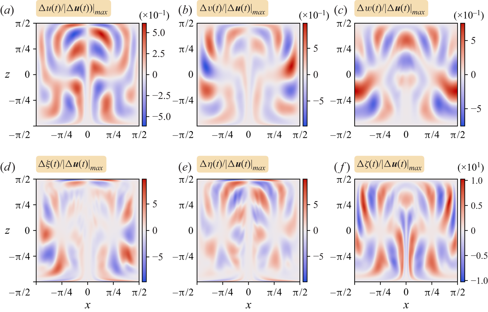
Figure 5. Slice plots in the  $xz$-plane at $y=0$ of the velocity and vorticity field component differences between $t = 50$ and $t = 0$ normalised by the maximum magnitude of the velocity field difference $\Delta \boldsymbol {u}(t) = \boldsymbol {u}(t) - \boldsymbol {u}(0)$.
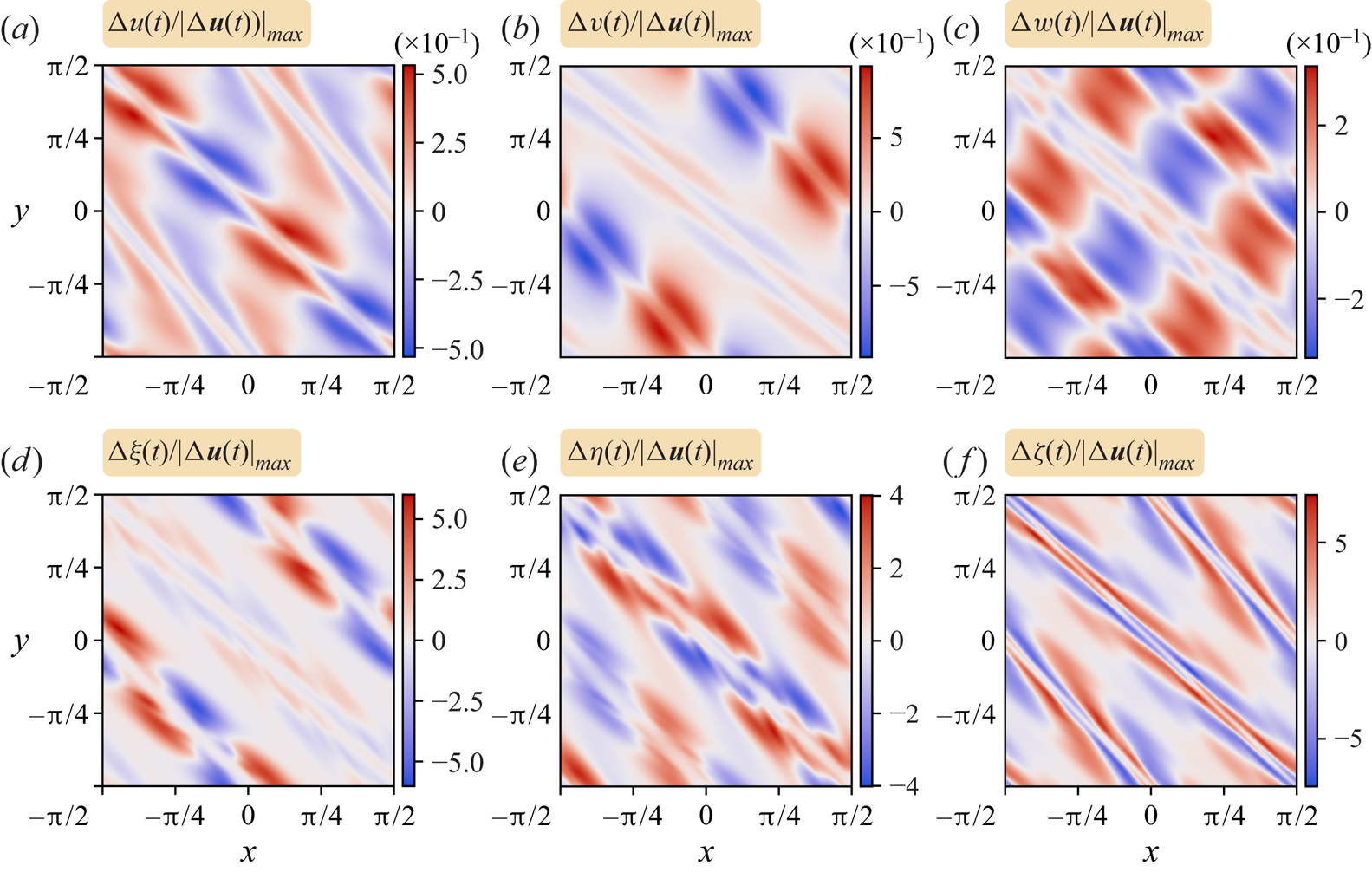
Figure 6. Slice plots in the  $xy$-plane at $z=0$ of the velocity and vorticity field component differences between $t = 50$ and $t = 0$ normalised by the maximum magnitude of the velocity field difference $\Delta \boldsymbol {u}(t) = \boldsymbol {u}(t) - \boldsymbol {u}(0)$.

Figure 7. Evolution of the r.m.s. of the magnitude of the velocity difference during the instability. The estimated growth rate of the linear instability is approximately  $0.583\pm 0.016$.
4.4. Flow evolution characteristics
4.4.1. Vorticity magnitude
Arguably, vorticity  $\boldsymbol {\omega }$ is the most important dynamical variable in Euler flows, owing to the fact that vortex lines are transported materially, conservatively, like infinitesimal line elements. Numerically, it is impossible to achieve this ideal behaviour due to the need for dissipation to preserve numerical stability, yet vorticity remains an important quantity for understanding the structure and evolution of the flow.
Figure 8 shows a 3-D view of the vorticity magnitude at various representative times in the evolution. The initial domain-scale field intensifies and collapses into narrow sheets and tubes occupying only 20 % of the domain (where  $|\boldsymbol {\omega }| > | \boldsymbol {\omega }|_{rms}$) by around $t=60$; such sparsely distributed flow structures are generic features of high Reynolds number 3-D turbulence (see e.g. Ishida, Davidson & Kaneda Reference Ishida, Davidson and Kaneda2006; Davidson Reference Davidson2015, and references therein). For $t<60$ approximately, the most intense structures emerge in the middle part of the $z$ range, away from the boundaries. At later times, the situation reverses, with the boundaries and near-boundary regions exhibiting the most intense structures, mainly taking the form of vortex tubes (the structure of the field does not change appreciably after $t=70$). Notably, the intense boundary vorticity emerges during the decay period when both the kinetic energy and enstrophy decrease sharply (see figure 4). The boundaries appear to reduce the decay of vorticity there relative to the interior, likely because they restrict the freedom for vortex lines to bend, twist and reconnect near the boundaries. On the other hand, with more freedom to deform, interior vortex lines more frequently reconnect and hence dissipate, accelerating the decay there.
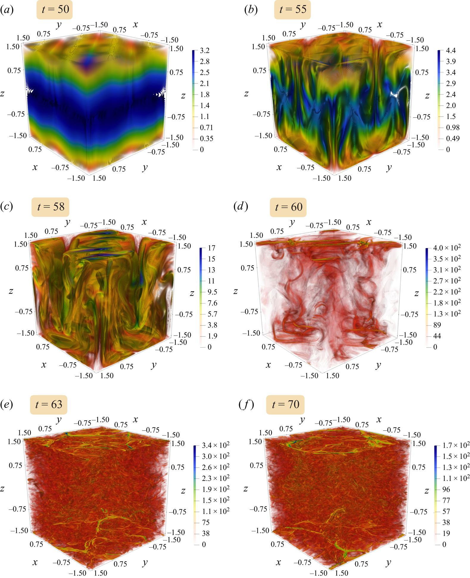
Figure 8. Iso-surfaces of the vorticity magnitude at selected times. Low field levels are made transparent to be able to see the high-intensity structures (see colour bars). The highest magnitudes are shown in blue rather than red as this allows one to better distinguish flow features. Note that the colour map range varies with each time frame. See supplementary movie 1 available at https://doi.org/10.1017/jfm.2022.1007 for an animation of the vorticity magnitude evolution. See also supplementary movie 2 for a  $360^\circ$ rotating animation at $t = 63$.
Alternative views showing 2-D slices of the vorticity magnitude evolution are provided in figure 9 for  $y=0$, in figure 10 for $z=0$, and in figure 11 for $z={\rm \pi} /2$ (the top boundary). Note that in each figure, (a–c) use a linear scale, while (d–f) use a log scale to improve the visualisation of the field, which at these times contains highly localised intense structures. As is evident in all these images, the flow breaks down first by forming sheets, surfaces of high-intensity vorticity, then these sheets break down into tubes and other small-scale structures that subsequently dissipate through reconnection and hyperdiffusion.
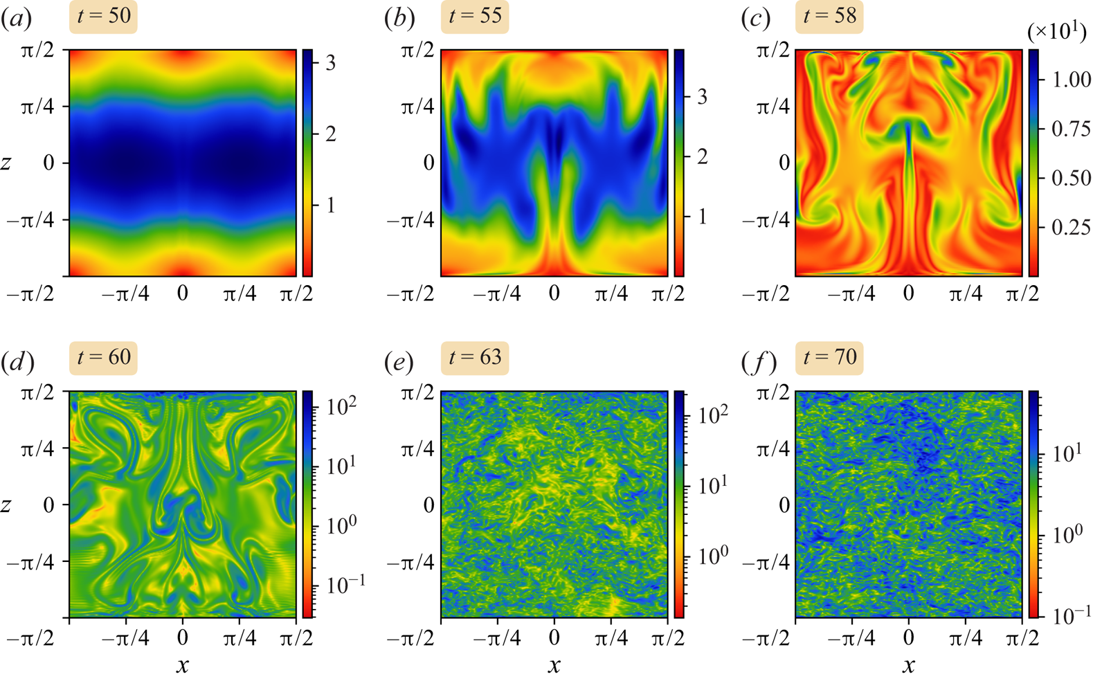
Figure 9. Cross-sections of the vorticity magnitude in the  $xz$-plane at $y = 0$ at selected times. Panels (d–f) use a log scale.

Figure 10. Cross-sections of the vorticity magnitude in the  $xy$-plane at $z = 0$ at selected times. Panels (d–f) use a log scale.
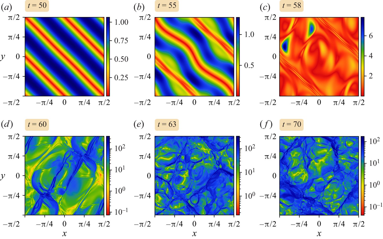
Figure 11. Cross-sections of the vorticity magnitude at the upper free-slip boundary ( $z = {\rm \pi}/2$) at selected times. Panels (d–f) use a log scale.
In the  $y=0$ cross-section in figure 9, the flow maintains approximate symmetry in $x$ until around $t=60$, but thereafter rapidly breaks down into small-scale turbulence. High-intensity structures are distributed throughout the domain, but there is evidence for boundary intensification especially in the image for $t=60$ (see top boundary region). The transition to small-scale turbulence is rapid, occurring between only $t=60$ and $63$. Thereafter, the flow remains qualitatively similar while decaying in amplitude, albeit more slowly near the boundaries.
In the (horizontal)  $z=0$ cross-section, in figures 10(a–c) one can see the progressive growth of wave-like disturbances and their subsequent overturning or buckling. This accentuates by $t=60$, by which time the maximum vorticity magnitude has grown by a factor of $5$ in only two units of time (note the log scaling used in figures 10d–f). As the flow breaks down into turbulence by $t=63$, which is about the time of peak enstrophy, there is a further 50 % growth in vorticity. The flow then decays sharply while approximately maintaining the complex form seen at $t=70$.
At the upper boundary  $z={\rm \pi} /2$ (cf. figure 11), the flow is hardly perturbed at $t=50$ compared to flow structure seen in the other cross-sections. Thereafter, the instability appears to spread to the boundaries, inducing a large-scale wave down the main diagonal $y=-x$ by $t=55$, and a weaker secondary disturbance along $y=\pm {\rm \pi}/2-x$. The large-scale wave then overturns by $t=58$, producing a complex but moderate-scale pattern, while the secondary disturbances reduce in scale but remain closely parallel to the lines $y=\pm {\rm \pi}/2-x$ (the fine-scale variations could be an artefact of hyperviscosity). For $t\geq 60$, the vorticity field collapses in scale predominantly along fronts (the intense blue regions seen in these plots). If a linear scale were used, then only the fronts would be visible in these images (see e.g. the helicity density $\boldsymbol {u}\boldsymbol {\cdot }\boldsymbol {\omega }$ below).
4.4.2. Enstrophy production
To better understand the nature of the instability and specifically the vorticity dynamics, we follow Tsinober, Kit & Dracos (Reference Tsinober, Kit and Dracos1992), Tsinober, Shtilman & Vaisburd (Reference Tsinober, Shtilman and Vaisburd1997) and Vincent & Meneguzzi (Reference Vincent and Meneguzzi1994), and quantify the enstrophy production rate  $\upsilon$, considering how it changes over the course of the instability and its behaviour near the boundaries. The enstrophy production rate is defined by
 \begin{equation} \upsilon=\upsilon_1+\upsilon_2+\upsilon_3, \quad\mathrm{where}\ \upsilon_i=\lambda_i(\boldsymbol{\omega}\boldsymbol{\cdot}\boldsymbol{e}_i)^2, \end{equation}
and where  $\lambda _1\geq \lambda _2\geq \lambda _3$ are the (real) eigenvalues of the symmetrised strain matrix $\tfrac 12(\boldsymbol {\nabla }\boldsymbol {u}+\boldsymbol {\nabla }\boldsymbol {u}^{\rm T})$, while $\boldsymbol {e}_1$, $\boldsymbol {e}_2$ and $\boldsymbol {e}_3$ are the corresponding normalised eigenvectors. Physically, the $\lambda _i$ are stretching rates along the three principal (orthogonal) directions $\boldsymbol {e}_i$. The enstrophy production rate is separated into three parts to understand which contributes most to enstrophy production. Since $\boldsymbol {\nabla }\boldsymbol {\cdot }\boldsymbol {u}=0$, it follows that $\lambda _1+\lambda _2+\lambda _3=0$, and moreover that $\lambda _1$ is always positive and $\lambda _3$ is always negative. It then follows that $\upsilon _1>0$ and $\upsilon _3<0$. The middle eigenvalue can have either sign, so $\upsilon _2$ is sign-indefinite.
Previous studies of homogeneous turbulence like Tsinober et al. (Reference Tsinober, Kit and Dracos1992, Reference Tsinober, Shtilman and Vaisburd1997), Vincent & Meneguzzi (Reference Vincent and Meneguzzi1994), Ishida et al. (Reference Ishida, Davidson and Kaneda2006) and Davidson (Reference Davidson2015) (and references therein) have often found alignment of the middle eigenvector  $\boldsymbol {e}_2$ with vorticity $\boldsymbol {\omega }$, resulting in comparable values of $\upsilon _1$ and $\upsilon _2$, despite the fact that $\lambda _1$ is often much larger than $\lambda _2$. This implies that enstrophy growth, or vorticity intensification, is only partly due to vortex stretching (along $\boldsymbol {e}_1$). The other contribution is the formation of vortex sheets (flattened structures), which undergo a shear instability and roll up into vortex tubes, evidenced by comparably large values of $\upsilon _2$ (and compensating negative values of $\upsilon _3$). Indeed, Vincent & Meneguzzi (Reference Vincent and Meneguzzi1994) argue that this is the principal mechanism of vortex tube production in homogeneous turbulence.
For the Beltrami flow considered here, figure 12 shows the domain-mean values of the  $\upsilon _i$ over the period of instability growth, saturation and decay (beyond $t=70$, the $\upsilon _i$ continue to decay monotonically in magnitude). Our results indicate that, overall, vortex stretching is the dominant mechanism of enstrophy production in the flow, while flattening is perhaps half as strong. (Similar results were found by Vincent & Meneguzzi (Reference Vincent and Meneguzzi1994) for homogeneous turbulence, though they found $\upsilon _2 \approx 0.6\upsilon _1$.) Notably, $\upsilon _2$ and $\upsilon _3$ nearly cancel each other, though $\upsilon _3$ is marginally larger in magnitude since it results in an overall production rate $\upsilon <\upsilon _1$.

Figure 12. Evolution of the domain-averaged enstrophy production rates in the unstable Beltrami flow between  $t=50$ and $70$.
$70$.
To investigate the role of the boundaries, we next study the vertical profiles of the horizontal-mean enstrophy production rates in figure 13. Before the instability is noticeable,  $\upsilon _2$ is negligible compared to $\upsilon _1$ and $\upsilon _3$, which (necessarily) nearly cancel each other. By this stage, there is very little vorticity growth. The situation changes somewhat by $t=55$ since now $\upsilon _2$ becomes significant and is largely positive. Yet the net enstrophy production rate $\upsilon$ remains relatively small compared to any of the $\upsilon _i$. By $t=58$, there is a strong shift toward the boundaries, where $\upsilon _2$ – corresponding physically to the roll-up of vortex sheets – dominates. Despite this, in an integral sense (over $z$),
$z$),  $\upsilon _1$ remains larger than $\upsilon _2$. This shows that the boundaries dramatically influence the behaviour of vorticity, consistent with the fact that the boundaries limit the bending of vortex lines, as pointed out above. The sharp variation of $\upsilon _2$ approaching each boundary (enhanced by the fact that $\lambda _2$ and $|\boldsymbol {\omega }|^2$ both rise steeply) demonstrates that the near-boundary regions have a fundamentally different character to the interior. This is undoubtedly associated with the free-slip impermeable boundary conditions used, where boundary stress (horizontal vorticity) is allowed. The boundaries act like a magnet for intense vorticity, and the near-boundary regions dominate the flow at late times.
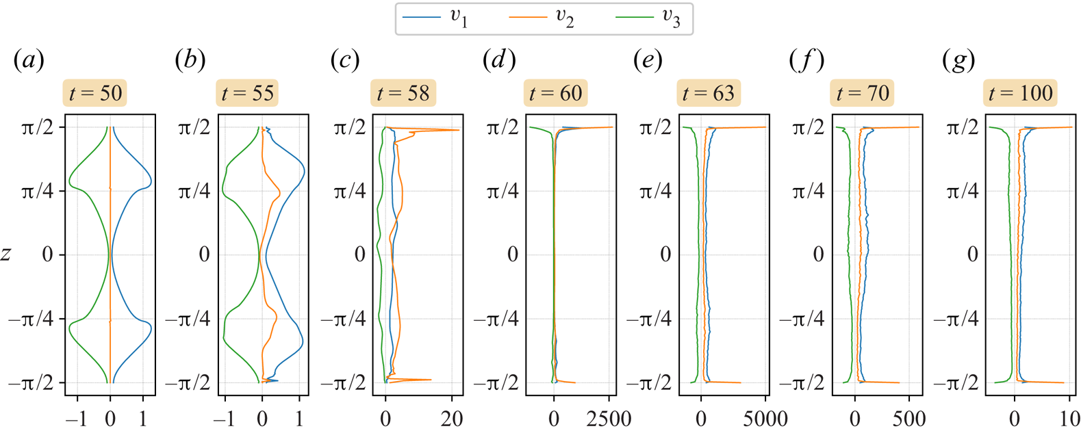
Figure 13. Vertical profiles of the horizontal-mean enstrophy production rates at selected times.
4.4.3. Helicity density
Beltrami flows with  $\boldsymbol {\omega }=\varkappa \boldsymbol {u}$ have a helicity density $h=\boldsymbol {u}\boldsymbol {\cdot }\boldsymbol {\omega }=\varkappa |\boldsymbol {u}|^2$, which is everywhere either non-negative ( $\varkappa >0$) or non-positive ( $\varkappa <0$). While the domain-average helicity $\mathcal {H} = \langle \boldsymbol {u}\boldsymbol {\cdot }\boldsymbol {\omega } \rangle$ is conserved in an inviscid flow (see Moreau Reference Moreau1961; Moffatt Reference Moffatt1969, Reference Moffatt2018), the helicity density $h$ is not constrained to lie within its initial range of values: $h$ is not materially conserved. Note that this conservation depends on $\zeta$ remaining zero on the boundaries, which is guaranteed by the form of the evolution equation (3.15a–c) (see also (3.16a–c)), since $w=\zeta =0$ on the boundaries initially. Unlike $\mathcal {K}$ and $\mathcal {\varUpsilon }$, note that $\mathcal {H}$ is not a positive-definite quantity.
The evolution of helicity  $\mathcal {H}$, the domain-average of $h$, is shown in figure 14. Like kinetic energy $\mathcal {K}$ (shown in figure 4a), helicity remains conserved until the flow breaks down into small-scale turbulence, beginning around $t=60$. In fact, $\mathcal {H}$ begins to decrease noticeably a few units of time earlier than $\mathcal {K}$ does, likely because $h=\boldsymbol {u}\boldsymbol {\cdot }\boldsymbol {\omega }$ is more sensitive to dissipation than is $\boldsymbol {u}\boldsymbol {\cdot }\boldsymbol {u}$. This is because $h$ involves a more highly differentiated field, vorticity, than the kinetic energy density, and vorticity is therefore more directly subject to dissipation (it has a shallower Fourier spectrum). By the end of the simulation at $t=100$, only $0.258\,\%$ of the initial helicity remains, whereas $0.896\,\%$ of the initial kinetic energy remains.
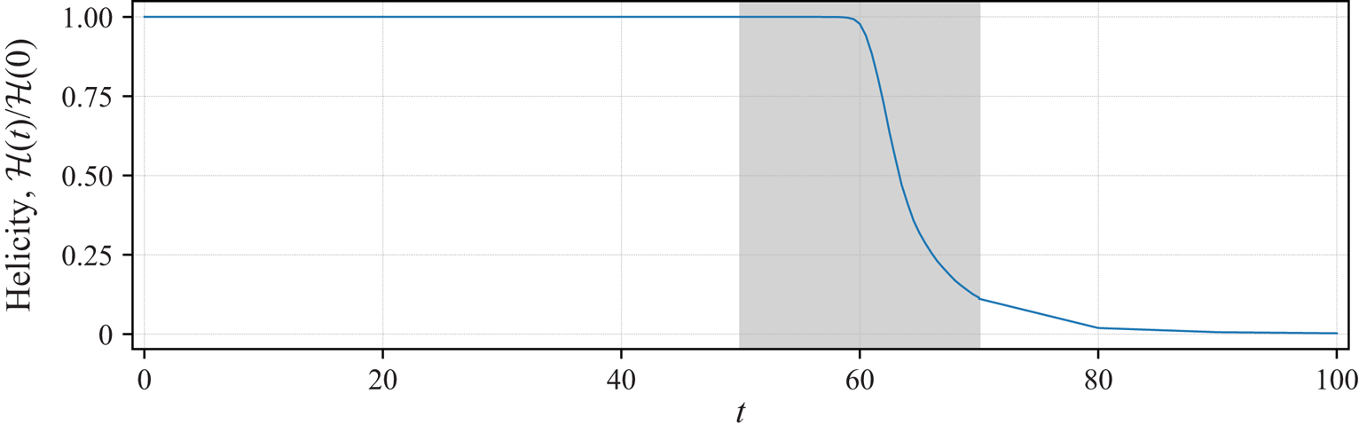
Figure 14. Evolution of the helicity  $\mathcal {H}$ (normalised by its initial value) in the unstable Beltrami flow. The shaded region between $t=50$ and $70$ uses data from a simulation restart at $t=50$ in order to save data at high frequency (every $0.5$ units of time, as opposed to every $10$ units of time). For the exact steady Beltrami flow, $\mathcal {H}=\mathcal {H}(0)=27/16$.
We next investigate the evolution of the helicity density field  $h$. A 3-D view is provided in figure 15 at the same times used to display the evolution of $|\boldsymbol {\omega }|$ in figure 8. At $t=50$, the $h$ field contains only weak disturbances and is positive almost everywhere. By $t=55$, the field has become much more distorted, with the first appearance of negative regions of $h$, most prominently on the lower boundary (these are seen in red). The negative regions grow by $t=58$ and amplify, and the volume occupied by high $|h|$ shrinks. This continues to $t=60$, when the high $|h|$ regions occupy only a small fraction of the domain; at this time, $|h_{min}|\approx 0.5h_{max}$, and $h_{max}$ has grown by more than a factor of $100$ since $t=50$. By $t=63$, $|h_{min}|$ surpasses $h_{max}$, but both values are decaying, and by $t=70$, $h_{max} > |h_{min}|$ again.

Figure 15. Iso-surfaces of helicity density  $\boldsymbol {u}\boldsymbol {\cdot }\boldsymbol {\omega }$ at selected times. A linear scale is used for each plot, but note that the minimum and maximum values vary.
At the upper boundary  $z={\rm \pi} /2$ (cf. figure 16), the evolution resembles the vorticity magnitude in figure 11, albeit $h$ has a more diffuse appearance compared to $|\boldsymbol {\omega }|$. At late times, $t\geq 60$, the boundaries exhibit sharp fronts in $h$ and $|\boldsymbol {\omega }|$, and across these fronts, the horizontal velocity field changes direction rapidly. This is illustrated in the zoomed $yz$-plane cross-section in figure 17, corresponding to the frontal feature in $|\boldsymbol {\omega }|$ seen near the left-hand edge of figure 11 at $t=63$ around $y=0$ (this feature can also be seen in $h$ in figure 16 but is less pronounced). Figure 17(a) shows vertical vorticity $\zeta$ (which remains zero on the boundaries); the front corresponds to high local $\zeta$. Figure 17(b) shows the flow in and out of the page; this reverses across the front. To the right of the front, there is relatively strong flow away from the boundary (downwards here). Apart from being upside down, the features seen here are strikingly reminiscent of atmospheric fronts, even though there is no buoyancy or stratification in the present case (see Clark et al. Reference Clark, Parker and Hanley2021, and references therein); however, the results may also be relevant to ocean fronts. Note that the high boundary vorticity associated with the front is entirely horizontal: vortex lines are everywhere tangent to the boundaries except at null points where $\boldsymbol {\omega }=\boldsymbol {0}$. The relatively high horizontal vorticity at and near the boundary generates a strong vertical shear of the velocity field, quantified next.
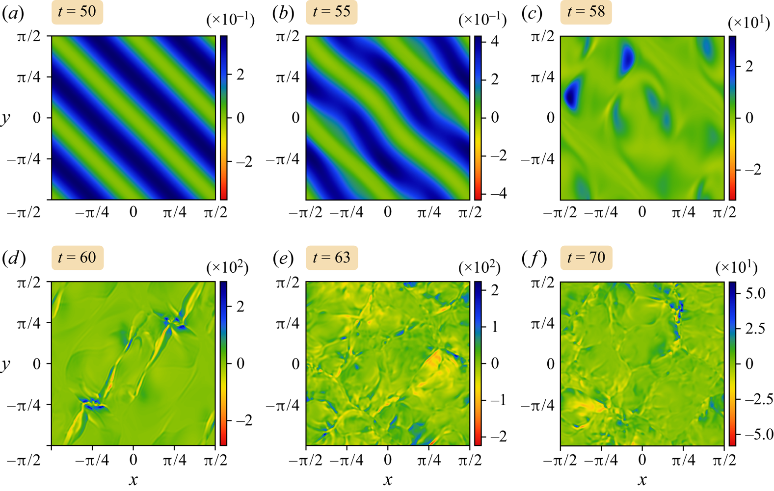
Figure 16. Cross-section of helicity density at the upper free-slip boundary ( $z = {\rm \pi}/2$) at selected times.
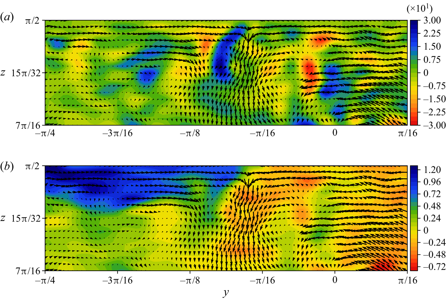
Figure 17. Contour plots of (a) vertical vorticity  $\zeta$, and (b) the $x$-component of the horizontal velocity $u$, in the cross-section $x=-3{\rm \pi} /8$ at time $t=63$. The domain is cropped horizontally (in $y$) to $[-{\rm \pi} /4, {\rm \pi}/16]$ and vertically to $[7{\rm \pi} /16, {\rm \pi}/2]$. The arrows show the vector field of the spanwise and vertical velocity components $(v, w)$. Note that positive $u$ is out of the page (in the direction of the positive $x$ axis).
4.5. Quantitative measures
Next, we examine various quantitative measures of the flow evolution. First, we discuss the vertical dependence of the flow to clarify the influence of the boundaries, then we turn to energy spectra, both 3-D and 2-D surface spectra.
4.5.1. Vertical dependence
The presence of vertical boundaries containing horizontal vorticity (stress) has a large impact on the flow evolution. In particular, after the flow breaks down and becomes turbulent (approximately  $t\geq 63$ in figures 9–11), the boundaries appear to contain the most intense vortical structures, and these resemble tubes lying adjacent to the boundaries. We quantify this in figure 18 by showing the vertical profile of the r.m.s. velocity and vorticity components at various times during the flow evolution. While the horizontal velocity displays only a modest upturn near the boundaries at late times, the horizontal vorticity is strongly intensified (the vertical components $w$ and $\zeta$ are both zero at the boundaries for all time). Moreover, the intensification occurs over a scale comparable to the grid spacing in $z$, a result found at all resolutions examined (not shown). This is consistent with the formation of vortex tubes at the smallest scale resolvable, and the protection afforded by the boundaries, which reduce the bending and twisting of vortex lines compared to the flow interior.
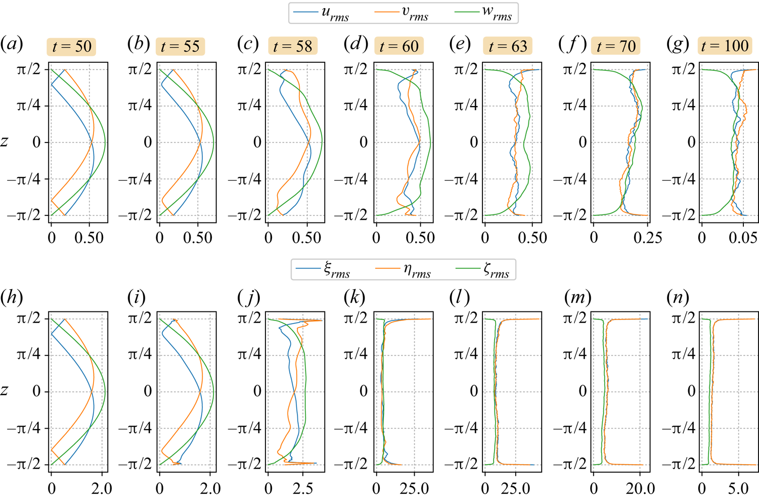
Figure 18. Vertical profiles of (a–g) r.m.s. velocity and (h–n) vorticity.
Notably, the vertical velocity and vorticity components  $w$ and $\zeta$ vary rapidly near the boundaries at late times. Large $w_z$ implies strong surface convergence and divergence, consistent with the observed behaviour of atmospheric fronts (see e.g. Clark et al. Reference Clark, Parker and Hanley2021). Large $\zeta _z$ implies that vortex lines near the boundaries are, in places, sharply bent away from the boundaries by the surface flow field. Again, this is consistent with the velocity field in the vicinity of fronts.
The surface intensification can also be seen in the time evolution of the r.m.s. values of the velocity and vorticity components at the boundaries and in the interior, shown in figure 19. Here, we have used the average of the two boundaries, and also an average of three interior planes  $z=\text {constant}$. The interior velocity components largely decay from the onset of the instability, but the boundary values grow by a factor 3–4 before decaying to comparable values at late times. Regarding the vorticity components, all grow significantly (except the boundary vertical vorticity, which remains zero), but the growth of horizontal vorticity at the boundaries is especially strong. Moreover, these are r.m.s. values; the maximum local value of $|\boldsymbol {\omega }|$ is more than 10 times larger – see figure 4(b).
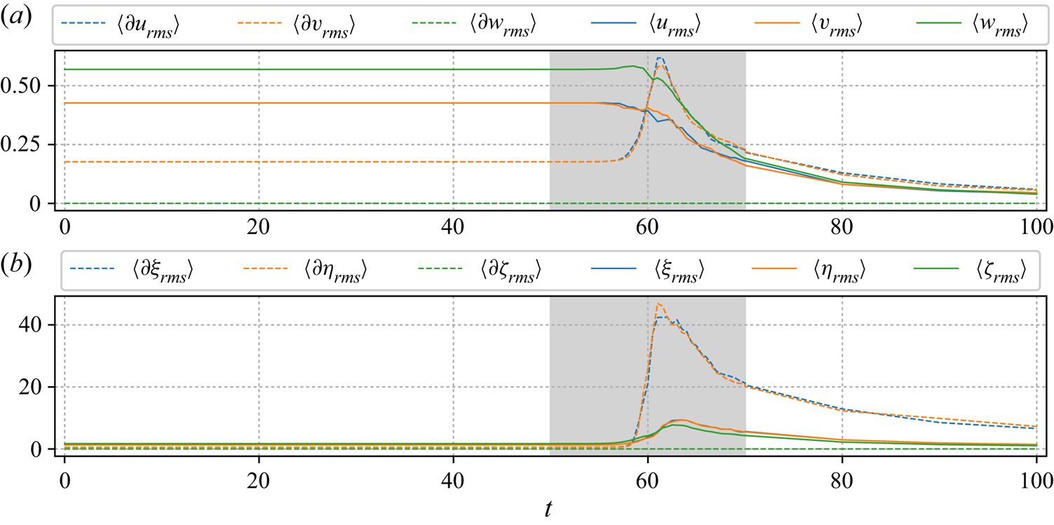
Figure 19. Evolution of the velocity and vorticity r.m.s. values at the boundary (dashed, with quantities prefaced by  $\partial$ in the legend) and in the interior (solid). The top and bottom boundary values are averaged. The interior values are averaged over the $xy$-planes at heights $z=-{\rm \pi} /4$, $0$ and ${\rm \pi} /4$. Note that in the shaded zone, the data are sampled every $0.5$ time units, whereas elsewhere else they are sampled every $10$ time units. There is a small discontinuity at $t=70$ due to the fact that the simulation was restarted at $t=50$ to provide higher data sampling.
4.5.2. Energy spectra
The distribution of energy with scale – the energy spectrum – is a widely used descriptor of turbulent flows. Power-law behaviour in wavenumber ranges may indicate self-similarity across scales, as postulated by Kolmogorov (Reference Kolmogorov1941) and Onsager (Reference Onsager1945), as well as a direct energy cascade process in which nonlinear interactions strongly excite progressively smaller scales. In physical space, this is manifest by the formation of intense vortical structures, predominantly sheets and tubes, whose existence, however, is associated with ‘intermittency’ and a departure from the self-similarity envisioned originally (see Davidson Reference Davidson2015, and references therein).
In the present context, the flow is not isotropic and is highly influenced by the boundary. Spectra are less useful as a result, since statistical properties of the flow vary with  $z$. We therefore present both the commonly exhibited 3-D energy spectrum and 2-D surface energy spectra at each boundary, which to our knowledge have never been presented before for a flow with non-zero boundary vorticity (stress). This is done in figure 20 at two times $t$ chosen when the kinetic energy $\mathcal {K}$ has decayed by factors of ${\rm e}$ and ${\rm e}^2$ from its initial value. At these times, the flow is turbulent and decaying. The 3-D spectrum in figure 20(a) is seen to steepen in time. At early times, there is a range that is steeper than the classical $|\boldsymbol {K}|^{-5/3}$ prediction (where $\boldsymbol {K}=(k,l,m)$ is the 3-D wavevector). This may be associated with a pulse in energy flowing downscale following the breakdown of the flow into turbulence shortly before. However, we remark that the present resolution is too low to obtain clear scaling ranges in the data. The 2-D surface spectra in figures 20(b,c), for $z=-{\rm \pi} /2$ and ${\rm \pi} /2$, respectively, exhibit a scaling much closer to $|\boldsymbol {k}|^{-5/3}$ (especially in the case of the upper more active surface). Arguably, the 3-D spectrum is less informative, and perhaps even inappropriate, given the significant vertical dependence of the flow statistics.
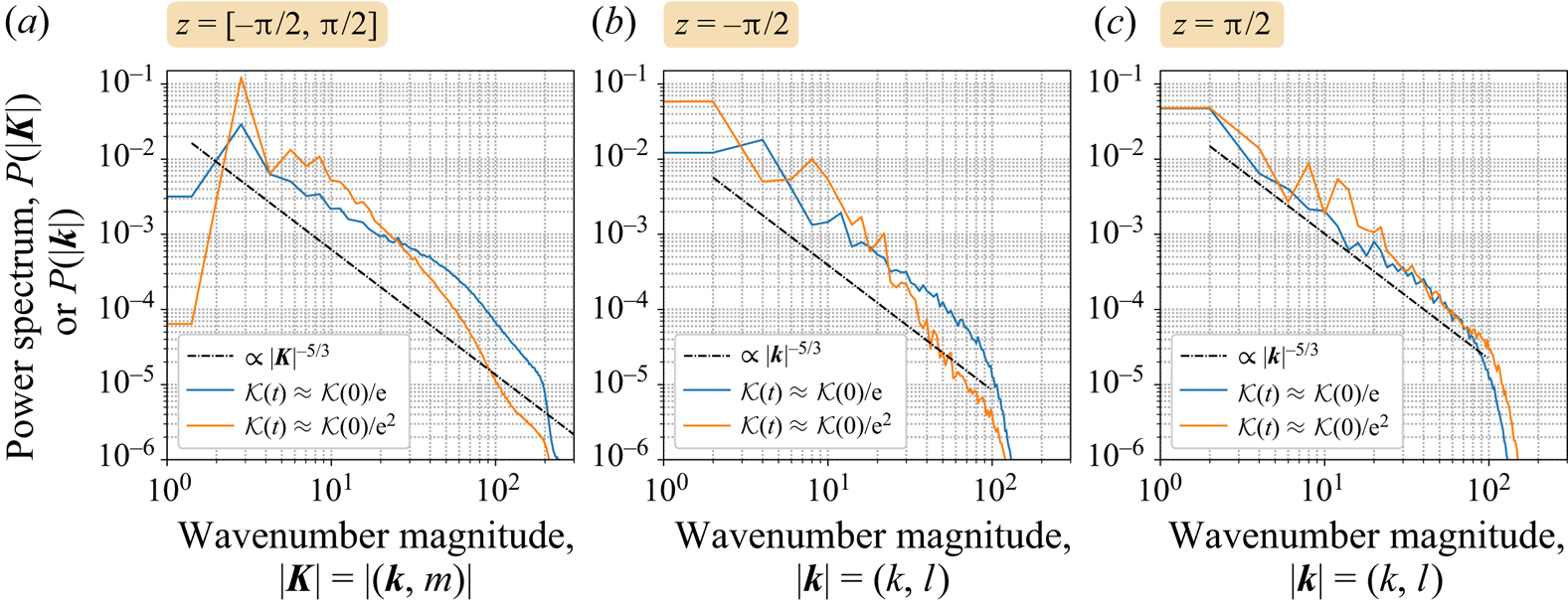
Figure 20. Energy spectra at  $1/{\rm e}$ ( $t\approx 65.5$) and $1/{\rm e}^2$ ( $t\approx 70.0$) decay for grid resolution $256^3$ cells. The power-law decay is steeper compared to $-5/3$, as theorised by Kolmogorov (Reference Kolmogorov1941). The $y$ axis is cut off at $10^{-8}$.
5. Discussion
We have developed a novel numerical approach to simulate nearly inviscid 3-D flows in a horizontally periodic domain confined between two parallel free-slip impermeable boundaries. In contrast to common practice in past studies of channel flows, Couette flows and surfaces with free-slip boundaries, we do not enforce stress-free conditions in conjunction with free-slip boundaries. Stress-free conditions imply vanishing horizontal vorticity at the boundaries, which is overly restrictive – particularly in density-stratified flows where horizontal vorticity is generated by horizontal density variations. The stress-free assumption is tantamount to requiring the vertical derivatives of the horizontal velocity components to vanish at the boundaries, an assumption that violates the behaviour of the Beltrami flows studied herein.
Without this assumption, the only boundary condition left is no normal flow at the boundaries (here, vanishing vertical velocity). This weakened boundary condition, however, makes the use of a standard pseudo-spectral method with 3-D hyperdiffusion infeasible, since it magnifies errors near the boundaries and here results in a non-physical growth in energy after the flow destabilisation and breakdown into turbulence. The method developed circumvents this problem by applying hyperdiffusion only horizontally, and by evolving the prognostic variables in, as we say, mixed spectral space where the boundary-induced flow is represented in semi-spectral space (extended into the domain using harmonic solutions of Laplace's equation), and where the remaining interior flow (which vanishes at both boundaries) is represented in full spectral space but using a sine series in  $z$ compatible with the Dirichlet boundary conditions that apply. An advantage is that this decomposition allows one to solve the inversion problem for the velocity field given the vorticity field, while satisfying the one boundary condition for the vertical velocity.
We have investigated the stability of an exact solution of the Euler equations, namely a Beltrami flow with vorticity proportional to velocity initially. Such a flow has non-zero horizontal vorticity (stress) on the upper and lower impermeable boundaries (the horizontal boundaries are taken to be periodic). Here, we have studied one of the simplest Beltrami flows in a wide class of such flows, namely a flow with the slowest non-trivial variation in each coordinate direction. From weak numerical noise, we find that the flow destabilises in a well-defined way, with the strongest perturbations located away from the boundaries in the early stages of instability growth. The perturbations grow approximately exponentially, as expected from a standard linear stability analysis, and eventually nonlinearity becomes important. Then vorticity grows rapidly through the formation of vortex sheets, their roll-up into tubes, and the stretching of these tubes, as quantified by examining the enstrophy production rates along the principal strain axes. Similar to what is found for homogeneous turbulence by Vincent & Meneguzzi (Reference Vincent and Meneguzzi1994), we find that enstrophy production by stretching along the principal strain axis is only approximately twice as large as that occurring along the intermediate strain axis. The latter is associated with vortex sheet production (flattening), shear instability, and roll-up into vortex tubes. This is significant because the principal stretching rate is typically much larger than the intermediate one. We have also examined the role of the boundaries by considering the vertical profile of the horizontal-mean enstrophy production rates. This reveals a fundamental change in behaviour: enstrophy production in the direction of the intermediate strain axis greatly exceeds that occurring by vortex stretching along the principal strain axis. The near-boundary regions dominate the flow at late times, with the highest vorticity magnitudes occurring on the boundaries, where the vorticity is entirely horizontal (the vertical component remains zero at all times). Vortex lines are more restricted from deforming near the boundaries, while they are free to deform in all directions in the interior. We argue that this enhances dissipation in the interior relative to the boundaries, leading to a dominance of the near-boundary regions. Indeed, our results suggest studying a simpler fluid model having no interior vorticity at all, but vortex sheets on the boundaries. Would this model reproduce, for example, the same energy spectra found here?
In the near future, we will implement the present numerical method in a hybrid Eulerian–Lagrangian code for simulating inviscid, incompressible, rotating density-stratified flows, extending the 2-D code developed by Frey et al. (Reference Frey, Dritschel and Böing2022). This hybrid code will make use of space-filling, subgrid-scale ellipsoidal parcels to represent all dynamical (prognostic) variables, and will avoid the need for hyperdiffusion. Instead, mixing will be done more naturally by the splitting and merging of parcels at subgrid scales. This approach enables a much higher effective resolution for the same basic grid resolution than a pseudo-spectral method (Frey et al. Reference Frey, Dritschel and Böing2022), and moreover guarantees monotonicity of tracers, an important requirement in realistic applications to atmospheric and oceanic dynamics.
Another topic worth investigating is the evolution of the magnetised Beltrami flow derived in § 2.2. A magnetic field can be stabilising since magnetic field lines resist twisting and stretching due to magnetic tension (see Dritschel, Diamond & Tobias Reference Dritschel, Diamond and Tobias2018, and references therein). This tension is reduced as magnetic diffusivity is increased, since field lines can more easily reconnect and cross-diffuse. The key controlling parameter appears to be  $\gamma =c\sqrt {{Rm}}$, where $c$ is the ratio of the magnetic and velocity field amplitudes, and ${Rm}=U/(\varkappa \nu _B)$ is the magnetic Reynolds number ( $U$ is the amplitude of the velocity field, taken to be unity in this paper). It is anticipated that magnetised Beltrami flows with $\gamma ={{O}}(1)$ or greater will be stable, but this is left to future work.
There are many potential applications of the numerical approach developed here (and its hybrid Lagrangian–Eulerian extension mentioned above). One concerns simulating and studying moist atmospheric convection, specifically cumulus convection, and the role played by vorticity. This builds on earlier work using Lagrangian cloud parcels (Böing et al. Reference Böing, Dritschel, Parker and Blyth2019), but here we plan to represent those parcels by deformable ellipsoids that mix by splitting and merging. Enabling stress on the lower boundary is essential for implementing buoyancy fluxes due to inhomogeneous surface heating. Similarly, this approach may be useful for studying mesoscale and sub-mesoscale turbulence near the ocean surface, where boundary stress is commonly created by both wind and thermal forcing. We can also foresee wider applications in magnetohydrodynamics and in plasma physics (see Tobias Reference Tobias2021).
Supplementary movies
Supplementary movies are available at https://doi.org/10.1017/jfm.2022.1007.
Acknowledgements
We thank S. Böing and A. Pumir for their helpful suggestions.
Funding
This research is supported by the UK Engineering and Physical Sciences Research Council (grant no. EP/T025301/1).
Declaration of interests
The authors report no conflict of interest.
Author contributions
D.D.: funding acquisition, conceptualisation, methodology, data analysis, writing. M.F.: methodology, literature research, software, data acquisition, data analysis, visualisation, writing.
Appendix A. Code availability and third party libraries
The source code is publicly available on GitHub. To reproduce the results, use version 0.0.6 (see Frey & Dritschel Reference Frey and Dritschel2022).
The program depends on NetCDF [C version 4.8.1 and Fortran version 4.5.4]. The visualisation is done with ParaView [version 5.10.1] (Ahrens, Geveci & Law Reference Ahrens, Geveci and Law2005; Ayachit Reference Ayachit2015) and Python (version 3.9.13), including NumPy [version 1.22.3] (Harris et al. Reference Harris2020), NetCDF4 [version 1.6.0] (Whitaker et al. Reference Whitaker2020), Matplotlib [version 3.5.2] (Caswell et al. Reference Caswell2022) and colorcet [version 3.0.0] (Bednar et al. Reference Bednar, Signell, Bowen, Liquet, Ball, Stevens, Pittman, Sutherland, Pevey and Kats2021).
Appendix B. Vorticity inversion test examples
Here, we demonstrate the accuracy and convergence of the vorticity inversion procedure detailed in § 3.2 by means of five examples. The first example is the Beltrami flow itself, given in (4.1), which we will refer to as  $\boldsymbol {\omega }_1$ in the remainder of this Appendix. The second example,
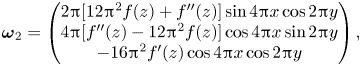 \begin{equation} \boldsymbol{\omega}_2 = \begin{pmatrix} 2{\rm \pi} [12{\rm \pi}^2 f(z) + f''(z)] \sin 4{\rm \pi} x \cos 2{\rm \pi} y \\ 4{\rm \pi} [f''(z) - 12{\rm \pi}^2 f(z)] \cos 4{\rm \pi} x \sin 2{\rm \pi} y \\ - 16{\rm \pi}^2 f'(z) \cos 4{\rm \pi} x \cos 2{\rm \pi} y \end{pmatrix}, \end{equation}
includes a cubic variation  $f(z) = 2z - z^2 - z^3$ with first and second derivatives denoted by $f'(z)$ and $f''(z)$, respectively. The corresponding velocity field is
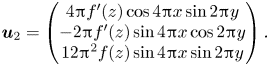 \begin{equation} \boldsymbol{u}_2 = \begin{pmatrix} 4{\rm \pi} f'(z) \cos 4{\rm \pi} x \sin 2{\rm \pi} y \\ -2{\rm \pi} f'(z) \sin 4{\rm \pi} x \cos 2{\rm \pi} y \\ 12{\rm \pi}^2 f(z) \sin 4{\rm \pi} x \sin 2{\rm \pi} y \end{pmatrix}. \end{equation}
The last three examples are horizontal shear flows ( $v = w = 0$) with a linear, quadratic and cubic vertical dependence,
 \begin{equation} u_3 = z - 1/2, \quad u_4 = z^2 - 1/3 \quad\text{and}\quad u_5 = z^3 - 1/4, \end{equation}
and therefore  $\xi = \zeta = 0$, with $y$ vorticity
 \begin{equation} \eta_3 = 1\,, \quad \eta_4 = 2z \quad\text{and}\quad \eta_5 = 3z^2. \end{equation}
Examples 2–5 are studied in the domain  $x,y \in [-\tfrac 12,\tfrac 12]$, $z \in [0,1]$.
Figure 21 summarises the resolution dependence of the maximum and r.m.s. errors. For the Beltrami flow as well as examples 3 and 4, where we have at most a quadratic  $z$-dependence, the inversion yields machine precision errors across all grid resolutions. Examples 2 and 5, which have a cubic $z$-dependence, converge at a cubic rate or better with the grid spacing. Quantitative results are provided in table 1.
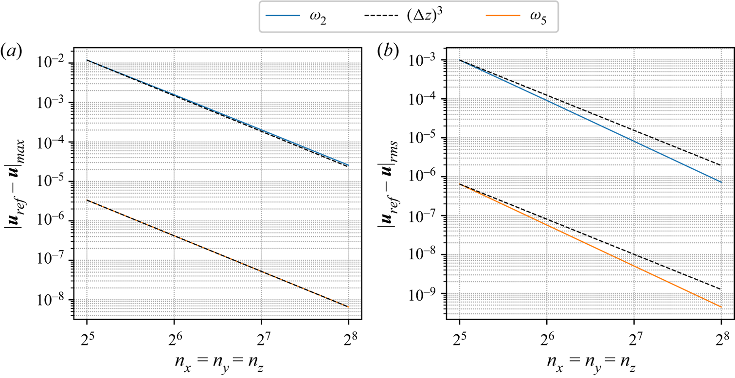
Figure 21. Convergence of the vorticity inversion algorithm for examples 2 and 5. The maximum error (a) converges at a cubic rate with the mesh spacing  $\Delta z$, while the r.m.s. error (b) converges slightly faster.
Table 1. Rows 1–4 refer to  $|\boldsymbol {u}_{{ref}}-\boldsymbol {u}|_{max}$; rows 5–8 refer to $|\boldsymbol {u}_{{ref}}-\boldsymbol {u}|_{rms}$.
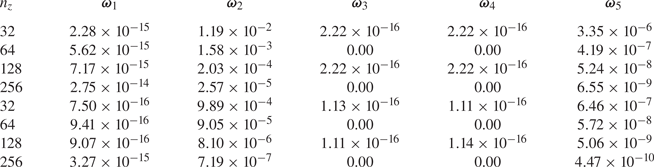
Appendix C. Boundary error with vertical dissipation and filtering
We demonstrate briefly the effect of vertical hyperdiffusion and filtering near a boundary with a one-dimensional example field (or function)  $q_0(z)$. Here, we consider
 \begin{equation} q_0(z) = (z + {\rm \pi}/2) [{\rm \pi}^2 - (z + {\rm \pi}/2)^2] \end{equation}
(other functions yield similar results), on which we apply the vertical hyperdiffusion operator
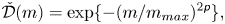 \begin{equation} \check{\mathcal{D}}(m) = \exp\{-(m/m_{max})^{2{\mathsf{p}}}\}, \end{equation}
with  ${\mathsf{p}}=3$ as in the main part of this paper, and the vertical filter (Hou & Li Reference Hou and Li2007)
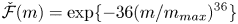 \begin{equation} \check{\mathcal{F}}(m) = \exp\{{-}36 (m/m_{max})^{36}\} \end{equation}
in spectral space. The hyperdiffusion damps the highest wavenumber  $m_{max}$ by a factor ${\rm e}^{-1}$, whereas the vertical filter damps the highest wavenumber by a factor ${\rm e}^{-36}$, which is approximately machine precision.
For this purpose, we first transform the function  $q_0(z)$, which vanishes on both boundaries, into spectral space using a Fourier (FFT) sine transform. Then we apply either of the two operators above and transform back into physical space. In figure 22, $q_f$ and $q_h$ denote the filtered and (hyper-)diffused functions, respectively. Results are presented for 128 and 256 grid cells. Hyperdiffusion results in an error near the surface that is approximately 2.5 times larger than from filtering. The lack of significant error at the lower boundary is due to the fact that $q'_0(z)$ also vanishes there. The weak vertical filtering error is undesirable but appears to have no impact on numerical stability. We have not been able to find a suitable alternative that is free of this artefact in the filtering literature.
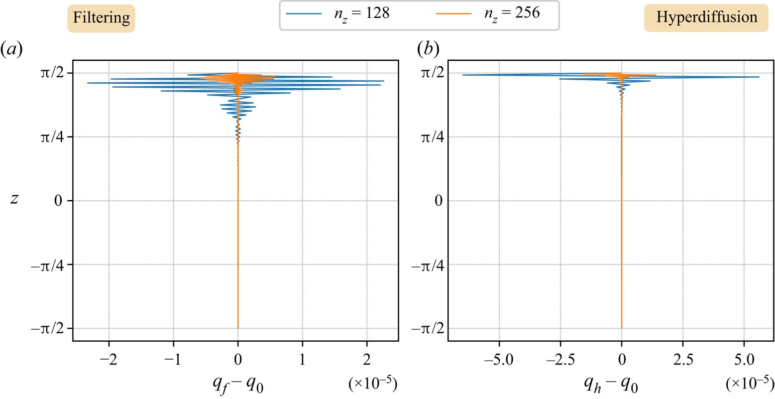
Figure 22. Errors due to (a) vertical filtering and (b) vertical hyperdiffusion, on a simple test function  $q_0(z)$ that vanishes at both boundaries. Two resolutions are shown, as indicated. The error is caused by the implicit boundary conditions assumed by the filtering and hyperdiffusion operators, boundary conditions that do not hold for the test function chosen (or in general).


 Open access