


1. Introduction
The flow of an incompressible fluid in a cavity of rectangular cross-section, driven by the tangential motion of one or more lids, is of general importance in fluid mechanics. The system encompasses several fundamental flow problems such as viscous corner eddies, corner singularities and hydrodynamic instabilities. The physics of lid-driven cavity flows has been covered in comprehensive reviews by Shankar & Deshpande (Reference Shankar and Deshpande2000) and Kuhlmann & Romanò (Reference Kuhlmann and Romanò2018). Another important aspect of the lid-driven cavity derives from testing numerical methods. Owing to its simple geometry with plane orthogonal boundaries, the mesh generation and implementation of Dirichlet boundary conditions is straightforward. Therefore, the system has evolved to one of the main benchmarks for numerical solvers.
Historically, the first two-dimensional steady flow computations are due to Kawaguti (Reference Kawaguti1961) and Burggraf (Reference Burggraf1966) who used finite-difference schemes on an  $11\times 11$ and a $40\times 40$ tensor grid, respectively. As the computational resources increased, highly resolved benchmark data were obtained in the early 1980s by Ghia, Ghia & Shin (Reference Ghia, Ghia and Shin1982) and Schreiber & Keller (Reference Schreiber and Keller1983) who computed steady flows up to $\textit {Re}=10^4$. Later on, Botella & Peyret (Reference Botella and Peyret1998) employed a spectral method together with the singularity subtraction method (Botella & Peyret Reference Botella and Peyret2001) to avoid an excessive deterioration of the exponential convergence of the spectral method by the singular boundary condition. The same method has been employed by Albensoeder & Kuhlmann (Reference Albensoeder and Kuhlmann2005) to treat three-dimensional cavity flows, providing benchmark data for height-to-width $(\varGamma )$ and span $(\varLambda )$ aspect ratios $(\varGamma , \varLambda ) = (1,1)$, (1,2), (1,3), and (2,1).
While benchmark data having been gathered, the lid-driven cavity naturally served as a test bed for the development of numerical schemes. For instance, De Vahl Davis & Mallinson (Reference De Vahl Davis and Mallinson1976) examined several schemes for convection and their stability, Ku, Hirsh & Taylor (Reference Ku, Hirsh and Taylor1987) tested a pseudo-spectral Chebyshev method, and Tuann & Olson (Reference Tuann and Olson1978) reviewed different schemes for recirculating flows.
Meanwhile, experiments were carried out as well. Pan & Acrivos (Reference Pan and Acrivos1967) experimentally investigated the size of the laminar recirculating vortex as a function of the depth-to-width ratio of the cavity. Ground-breaking experimental studies at higher Reynolds numbers were carried out by Koseff et al. (Reference Koseff, Street, Gresho, Upson, Humphrey and To1983), Koseff & Street (Reference Koseff and Street1984a,Reference Koseff and Streetb,Reference Koseff and Streetc) and Prasad & Koseff (Reference Prasad and Koseff1989). They investigated a square cavity with a spanwise aspect ratio of three, driven on its top surface by a metal belt which was held flat. At a Reynolds number of  $\textit {Re}=3000$ the authors discovered three-dimensional Taylor–Görtler vortices which develop along the curved boundary layer next to the bottom corners of the cavity. Since these three-dimensional vortices cannot be represented by two-dimensional numerical simulations, the experimental discovery of Taylor–Görtler vortices stimulated further research on the laminar-turbulent transition.
The lid-driven cavity flow restricted to two dimensions becomes unstable to two-dimensional oscillatory perturbations at a relatively high Reynolds number. For a square cavity, Shen (Reference Shen1991) found a Hopf bifurcation at the critical Reynolds number  $\textit {Re}_c\approx 10^4$. However, due to the regularisation of the discontinuous boundary conditions implemented the critical Reynolds number was overestimated. Auteri, Quartapelle & Vigevano (Reference Auteri, Quartapelle and Vigevano2002b) obtained the more accurate value $\textit {Re}_c=8018.2\pm 0.6$. The limit cycle bifurcating from the steady basic state was computed by Auteri et al. (Reference Auteri, Quartapelle and Vigevano2002b), Peng, Shiau & Hwang (Reference Peng, Shiau and Hwang2003) and also by Bruneau & Saad (Reference Bruneau and Saad2006). The critical Reynolds number for two-dimensional flow was confirmed by linear stability analyses of Poliashenko & Aidun (Reference Poliashenko and Aidun1995), Fortin et al. (Reference Fortin, Jardak, Gervais and Pierre1997) and Sahin & Owens (Reference Sahin and Owens2003) who obtained $\textit {Re}_c=7763$, $\textit {Re}_c=8000$ and $\textit {Re}_c=8069.76$, respectively. Since the experimentally observed flow at these Reynolds numbers is already three-dimensional, the third dimension has to be necessarily taken into account.
Assuming a square cavity which is infinitely extended in the spanwise direction and allowing the perturbation flow to be three-dimensional, Ramanan & Homsy (Reference Ramanan and Homsy1994) predicted a linear stability boundary at  $\textit {Re}_c=594$ due to a stationary long-wavelength mode with wave number $k_c=2.15$ in the $z$-direction given in units of the inverse cavity depth. On the other hand, Ding & Kawahara (Reference Ding and Kawahara1999) (see also Ding & Kawahara Reference Ding and Kawahara1998) estimated the critical Reynolds number as $\textit {Re}_c=920$ due to an oscillatory mode with a wave number $k_c=7.4$. This contradiction was resolved by Albensoeder, Kuhlmann & Rath (Reference Albensoeder, Kuhlmann and Rath2001) who systematically computed the linear stability boundary as a function of the depth-to-width aspect ratio $\varGamma \in [0.2,4]$. Depending on $\varGamma$ they obtained four different critical modes, two stationary and two oscillatory ones, which were all of a centrifugal nature. For a square cavity with $\varGamma =1$, the critical mode corresponding to the Taylor–Görtler vortices observed experimentally by Koseff & Street (Reference Koseff and Street1984a) is stationary and has a short wavelength with $k_c=15.4$. This mode becomes critical at $\textit {Re}_c=786$. The numerical predictions of Albensoeder et al. (Reference Albensoeder, Kuhlmann and Rath2001) were later confirmed by careful experiments of Siegmann-Hegerfeld, Albensoeder & Kuhlmann (Reference Siegmann-Hegerfeld, Albensoeder and Kuhlmann2008); see also Siegmann-Hegerfeld (Reference Siegmann-Hegerfeld2010). For a square cavity, Theofilis, Duck & Owen (Reference Theofilis, Duck and Owen2004) numerically confirmed the results of Albensoeder et al. (Reference Albensoeder, Kuhlmann and Rath2001).
In this work we consider the stability of the steady flow in an infinitely extended cavity in which the flow is driven by a sliding lid which moves in its own plane, but with a velocity vector which also has a component in the span direction, i.e. which makes an angle  $\alpha$ with respect to the cross-sectional plane. The first investigations of obliquely driven cavity flow were due to Povitsky (Reference Povitsky2001) and Povitsky (Reference Povitsky2005), albeit for a finite-length cubic cavity. When the lid moves diagonally $(\alpha =45^\circ )$, the flow at moderate Reynolds numbers is steady and mirror symmetric. Due to the restricted geometry up- and downstream of the moving lid the flow in the cavity at yaw has more fine structure than the conventional flow in a cube when the lid moves parallel to one side wall (Sheu & Tsai Reference Sheu and Tsai2002; Feldman & Gelfgat Reference Feldman and Gelfgat2010; Kuhlmann & Albensoeder Reference Kuhlmann and Albensoeder2014; Lopez et al. Reference Lopez, Welfert, Wu and Yalim2017). By numerical simulation, Feldman (Reference Feldman2015) found a supercritical Hopf bifurcation in the obliquely driven cube with $\alpha =45^\circ$ in which the oscillatory part of the flow breaks the mirror symmetry with respect to the diagonal plane and arises as a streamwise vortex near the moving wall, centred on the diagonal plane and alternating its sense of rotation with time. The time-dependent perturbation flow has a quite complicated structure, originating from the intricate three-dimensional basic flow. Benchmark data for the critical Reynolds number for the diagonally driven cubic cavity flow were provided by Gelfgat (Reference Gelfgat2019) who found $\textit {Re}_c=2289.31$ (see also Feldman & Gelfgat Reference Feldman and Gelfgat2011), comparable in magnitude to the linear stability boundary in the classical lid-driven cube of $\textit {Re}_c=1919.51$ and $\textit {Re}_c=1919.37$ obtained by Kuhlmann & Albensoeder (Reference Kuhlmann and Albensoeder2014) and Gelfgat (Reference Gelfgat2019), respectively.
Despite extensive stability analyses of the classical lid-driven cavity, only Theofilis et al. (Reference Theofilis, Duck and Owen2004) have carried out a linear stability analysis of the flow in an infinitely extended rectangular cavity driven by an oblique motion of the lid. They scrutinised three different yaw angles,  $\alpha ={\rm \pi} /4$, ${\rm \pi} /2$ and $3{\rm \pi} /4$. For all yaw angles considered, the basic flow was found to be linearly stable at least up to $\textit {Re}=800$. In the present study it will be shown that these data must be corrected, because the two-dimensional flow turns out to become unstable already at much lower Reynolds numbers. Another aim of our investigation is to more systematically calculate the linear stability boundary as a function of the angle the lid velocity makes with the walls, and to uncover the mechanics of the critical modes.
After introducing the mathematical formulation of the problem in § 2, the numerical solution methods are discussed in § 3 and the codes are verified against data available in the literature. Our findings for a square cavity  $(\varGamma =1)$, as well as for a representative shallow $(\varGamma =0.5)$ and a deep cavity $(\varGamma =2)$ are presented in § 4 and the connection of the critical curves along $\alpha$ is demonstrated. Flow structures and instability mechanisms are investigated by considering the local and global production rates of kinetic perturbation energy. Finally, limiting cases of the yaw angle and common properties of the instabilities found are discussed in § 5.
2. Formulation of the problem
We consider the incompressible flow of a Newtonian fluid with density  $\rho$ and kinematic viscosity
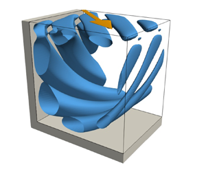
  $\nu$ in a rectangular cavity (figure 1). The depth $d$ in the $y$-direction and the width $h$ in the $x$-direction define the aspect ratio $\varGamma =d/h$. In the $z$-direction the cavity is assumed to be infinitely extended. The origin of the coordinate system is placed in the centre of the $(x,y)$ cross-section. The flow is driven by the steady tangential motion of a lid at the top $y=d/2$ of the cavity. The lid velocity vector ${\boldsymbol {U}} = U(\cos \alpha {\boldsymbol {e}}_x + \sin \alpha {\boldsymbol {e}}_z)$, where ${\boldsymbol {e}}_x$ and ${\boldsymbol {e}}_z$ are the unit vectors in the $x$ and $z$ directions, respectively, is inclined with respect to the $x$ axis with inclination (or yaw) angle $\alpha$.

Figure 1. Geometry of the problem with Cartesian coordinates centred in the cavity  $(O)$ and a lid (dark grey) moving tangentially with velocity ${\boldsymbol {U}}$ under an angle $\alpha$ with respect to the $x$ axis.
Using the length, time, velocity and pressure scales  $h$,
$h$,  $h^2/\nu$, $\nu /h$ and $\rho \nu ^2 / h^2$, respectively, the fluid flow is governed by the non-dimensional Navier–Stokes and continuity equations
 $$\begin{gather} \frac{ \partial {\boldsymbol{u}}}{\partial t} + {\boldsymbol{u}}\boldsymbol{\cdot}\boldsymbol{\nabla} {\boldsymbol{u}}={-}\boldsymbol{\nabla} p + \nabla^2{\boldsymbol{u}}, \end{gather}$$
 $$\begin{gather}\boldsymbol{\nabla}\boldsymbol{\cdot}{\boldsymbol{u}} = 0, \end{gather}$$
where  ${\boldsymbol {u}}({\boldsymbol {x}},t) =(u,v,w)$ is the velocity vector and $p({\boldsymbol {x}},t)$ the pressure field. Equations (2.1) must be solved subject to the boundary conditions
 $$\begin{gather} {\boldsymbol{u}} (x={\pm} 1/2) =0, \end{gather}$$
 $$\begin{gather}{\boldsymbol{u}}(y={-}\varGamma/2) = 0, \end{gather}$$
 $$\begin{gather}{\boldsymbol{u}}(y=\varGamma/2) = \textit{Re}(\cos\alpha,0,\sin\alpha)^\text{T}. \end{gather}$$
Furthermore, we consider the case of a vanishing pressure gradient in the  $z$-direction, $\partial p/\partial z = 0$. The problem is thus defined by three parameters: the aspect ratio $\varGamma$, the inclination angle $\alpha$ and the Reynolds number
 \begin{equation} \textit{Re}=\frac{Uh}{\nu}. \end{equation}
 Due to the translation invariance of the problem in  $z$ and $t$ the governing equations allow for a steady two-dimensional basic flow ${\boldsymbol {u}}_0(x,y)$ which only depends on $x$ and $y$.
$y$.
We are interested in the linear stability boundary, expressed by  $\textit {Re}_c(\varGamma ,\alpha )$, at which the two-dimensional basic flow becomes unstable to three-dimensional perturbations. Linearising (2.1) with respect to small perturbations of the basic flow yields the linear perturbation equations
 $$\begin{gather} \frac{ \partial {\boldsymbol{u}}}{\partial t} + {\boldsymbol{u}}_0\boldsymbol{\cdot}\boldsymbol{\nabla} {\boldsymbol{u}} + {\boldsymbol{u}}\boldsymbol{\cdot}\boldsymbol{\nabla} {\boldsymbol{u}}_0 ={-}\boldsymbol{\nabla} p + \nabla^2{\boldsymbol{u}}, \end{gather}$$
 $$\begin{gather}\boldsymbol{\nabla}\boldsymbol{\cdot}{\boldsymbol{u}} = 0, \end{gather}$$
where now  ${\boldsymbol {u}}$ and $p$ denote the deviations from the basic state.
Owing to the homogeneity in the  $z$-direction, these equations may be solved using normal modes
 \begin{equation} \left(\begin{matrix} {\boldsymbol{u}} \\ p \end{matrix}\right) = \left(\begin{matrix} \hat{{\boldsymbol{u}}} (x,y) \\ \hat{p}(x,y) \end{matrix}\right) \exp({\gamma t + \textrm{i} kz}) + \text{c.c.}, \end{equation}
where  $k\in \mathbb {R}$ is a real wave number, $\gamma =\sigma +\textrm {i}\omega \in \mathbb {C}$ a complex growth rate with real growth rate $\sigma$ and frequency $\omega$, and c.c. denotes the complex conjugate. Inserting this ansatz into the perturbations equations (2.4) we are left with
 $$\begin{gather} -\gamma \hat{u} = \left(u_0 \partial_x + v_0 \partial_y + \textrm{i} k w_0\right) \hat{u} + \left(\hat{u} \partial_x + \hat{v} \partial_y\right) u_0 + \partial_x \hat{p} - (\partial_x^2 + \partial_y^2 - k^2) \hat{u}, \end{gather}$$
 $$\begin{gather}-\gamma \hat{v} =\left(u_0 \partial_x + v_0 \partial_y + \textrm{i} k w_0 \right) \hat{v} + \left(\hat{u} \partial_x + \hat{v} \partial_y \right) v_0 + \partial_y \hat{p} - (\partial_x^2 + \partial_y^2 - k^2) \hat{v}, \end{gather}$$
 $$\begin{gather}-\gamma \hat{w} = \left( u_0 \partial_x + v_0 \partial_y + \textrm{i} k w_0 \right) \hat{w} + \left( \hat{u} \partial_x + \hat{v} \partial_y \right) w_0 + \textrm{i} k \hat{p} - (\partial_x^2 + \partial_y^2 - k^2) \hat{w}, \end{gather}$$
 $$\begin{gather}0 = \partial_x \hat{u} + \partial_y \hat{v} + \textrm{i} k \hat{w}. \end{gather}$$
Together with the boundary conditions  $\hat {{\boldsymbol {u}}}(x=\pm 1/2) = \hat {{\boldsymbol {u}}}(y=\pm \varGamma /2)=0$ this system of equations constitutes a generalized eigenvalue problem with eigenvectors $(\hat {{\boldsymbol {u}}},\hat p)$ and eigenvalues $\gamma$. The eigenvalues $\gamma (k,n;\varGamma ,\alpha ,\textit {Re})$ depend on the wave number $k$ of the disturbance, the three parameters $(\varGamma ,\alpha ,\textit {Re})$ and on the index $n$ numbering the discrete set of solutions for given $k$. For given $\varGamma$ and $\alpha$, neutral stability boundaries $\textit {Re}_n(k,n)$ are defined by $\sigma (\textit {Re})=0$. Finally, the critical Reynolds number $\textit {Re}_c$ is the lowest neutral Reynolds number, equivalent to $\max _{k,n}\sigma (\textit {Re})=0$.
3. Methods of solution
All differential equations are discretized with triangular elements on a rectangular domain  $(x,y)$ using the finite element library FEniCS (Alnaes et al. Reference Alnaes, Blechta, Hake, Johansson, Kehlet, Logg, Richardson, Ring, Rognes and Wells2015). To properly resolve the flow fields near the boundaries the mesh is refined towards all walls by subsequently doubling the number of grid points within 5 %, 1 % and 0.5 % of the width and the depth of the cavity. Taylor–Hood elements are employed which implement a quadratic interpolation for the velocity fields and a linear interpolation for the pressure.
3.1. Basic state
The steady two-dimensional flow  $({\boldsymbol {u}}_0,p_0)$ is computed using Newton–Raphson iteration already implemented in the FEniCS framework, which only requires the variational formulation and the boundary conditions. Absolute and relative convergence criteria based on the $L_2$ norm of the residuum are set to $10^{-10}$ and $10^{-8}$, respectively. During tracking of the stability boundary, the basic state calculation is typically terminated due to the absolute convergence criterion. The converged basic flow field enters the linear stability analysis parametrically.
3.2. Linear stability analysis
Once the basic state  $({\boldsymbol {u}}_0,p_0)$ is computed the linear stability equations (2.6) are solved on the finite element mesh for given $\alpha$, $\textit {Re}$ and $k$ using an implicitly restarted Arnoldi method implemented in ARPACK (Lehoucq & Salinger Reference Lehoucq and Salinger2001) and called within the subroutine eigs of SciPy. In order to ensure that the method captures all the eigenvalues of interest the dimension of the Krylov space is set to 300, while the number of converged eigenvalues required to assume convergence is set to 50. We noticed that when lowering both these numbers some eigenvalues might not be captured correctly.
To find the neutral curves a sensitivity-based algorithm has been developed which is detailed in Appendix A. The required first-order sensitivity of the eigenvalues with respect to wavelength variations is derived in Appendix B.
3.3. Code verification
In a first step a grid-convergence study for the critical Reynolds and wave numbers is carried out. Table 1 shows  $(\textit {Re}_c,k_c)$ as a function of the grid resolution for three aspect ratios $\varGamma$ and $\alpha =0^\circ$. Grid convergence is clearly obtained and the converged results compare very well, i.e. within 1 %, with the reference results of Albensoeder et al. (Reference Albensoeder, Kuhlmann and Rath2001). The data suggest that a basic mesh of $40 \times 40$ provides already very accurate results for $\varGamma =1$. Note the grid specified represents the grid with equidistant spacing, the actual grid used is refined towards the walls as specified above such that the formal $40\times 40$ resolution practically is made of 13 976 elements or 95 328 degrees of freedom. With similar arguments, the initial grids $40\times 80$ and $80\times 40$ for $\varGamma =2$ and $\varGamma =1/2$, respectively, are used for the stability analysis for $\alpha >0^\circ$.
Table 1. Critical Reynolds number  $\textit {Re}_c$ and wave number $k_c$ as functions of the grid resolution for $\alpha =0^\circ$. The column labelled ‘Grid’ refers to the initial grid size before refinement, $n_{T}$ denotes the number of triangles, while $n_{DOF}$ is the number of degrees of freedom.

To verify the growth rate  $\sigma$ and the oscillation frequency $\omega$ as functions of the wave number $k$, we consider $\varGamma =1$ and $\alpha =0^\circ$ for which reference data are available in the literature. To that end, the most dangerous mode has been computed for $\textit {Re}=200$ and $\textit {Re}=1000$. Figure 2 shows the growth rates and oscillation frequencies of the fastest growing mode for $\textit {Re}=200$ (dashed lines) and $\textit {Re}=1000$ (full lines) in comparison with the results of Ding & Kawahara (Reference Ding and Kawahara1999) ( $\square$) and Albensoeder et al. (Reference Albensoeder, Kuhlmann and Rath2001) ( $\circ$). For $\textit {Re}=200$, an excellent agreement is found for all $k$ considered, using the basic grid resolution of $40\times 40$. The numerical results for $\textit {Re}=1000$ also show a good agreement with the reference data for the frequency $\omega$. Agreement of the growth rate $\sigma$ obtained for the current resolution with the reference data is acceptable. Typically, our results are in-between the two reference data sets and tend to compare slightly better with those of Ding & Kawahara (Reference Ding and Kawahara1999) than with those of Albensoeder et al. (Reference Albensoeder, Kuhlmann and Rath2001).

Figure 2. (a) Growth rate  $\sigma =\textrm {Re}(\gamma )$ and (b) oscillation frequency $\omega =\textrm {Im}(\gamma )$ of the most dangerous mode for $\alpha =0^\circ$, $\varGamma =1$ for $\textit {Re} = 200$ (dashed lines) and $\textit {Re}=1000$ (full lines). Results are given for the base grid resolution of $40\times 40$ in comparison with data of Ding & Kawahara (Reference Ding and Kawahara1999) ( $\square$) and Albensoeder et al. (Reference Albensoeder, Kuhlmann and Rath2001) ( $\circ$).
3.4. Energy analysis
In order to understand the fundamental instability mechanisms it is helpful to evaluate the budget of the kinetic energy of the critical mode  ${\boldsymbol {u}}$. Taking into account the perturbation flow vanishes on the boundaries and the nonlinear term ${\boldsymbol {u}} \boldsymbol {\cdot } \boldsymbol {\nabla }{\boldsymbol {u}}$ is energy-preserving, the Reynolds–Orr equation can be written as (Albensoeder et al. Reference Albensoeder, Kuhlmann and Rath2001)
 \begin{equation} \frac{\textrm{d} E_{kin}}{\textrm{d} t} = \int_V \left[- {{\boldsymbol{u}}}\boldsymbol{\cdot} \left( {{\boldsymbol{u}}}\boldsymbol{\cdot}\boldsymbol{\nabla} {\boldsymbol{u}}_0\right) - \left(\boldsymbol{\nabla} {{\boldsymbol{u}}}\right)^2 \right] \textrm{d} V, \end{equation}
where  $E_{kin} = \int _V ({\boldsymbol {u}}^2/2) \,\textrm {d} V$ and $V$ is the volume occupied by the fluid over one period in $z$. The dissipation $D_* = \int _V (\boldsymbol {\nabla }{\boldsymbol {u}})^2\,\textrm {d} V \geqslant 0$ is positive and always contributes to a reduction of the kinetic energy. If the total energy production rate $I = -\int _V {{\boldsymbol {u}}} \boldsymbol {\cdot }( {{\boldsymbol {u}}}\boldsymbol {\cdot }\boldsymbol {\nabla } {\boldsymbol {u}}_0)$ overcomes the dissipation rate, the perturbation kinetic energy grows and the basic flow is unstable.
It is useful to decompose the perturbation flow  ${{\boldsymbol {u}}}$ into components parallel and perpendicular to the basic flow (Albensoeder et al. Reference Albensoeder, Kuhlmann and Rath2001) and define
 \begin{equation} {\boldsymbol{{u}}}_{{\parallel}} = \frac{\left({\boldsymbol{{u}}} \boldsymbol{\cdot} {\boldsymbol{u}}_0\right) {\boldsymbol{u}}_0}{{\boldsymbol{u}}_0^2} \quad \text{and} \quad {\boldsymbol{{u}}}_{{\perp}} = {\boldsymbol{{u}}} - {\boldsymbol{{u}}}_{{\parallel}} . \end{equation}
Inserting this decomposition in (3.1) and normalising all terms with  $D_*$ yields the following local dissipation and production terms:
 $$\begin{gather} d_* = \frac{1}{D_*} \left[ \boldsymbol{\nabla} \times ({\boldsymbol{{u}}}_{{\perp}} + {\boldsymbol{{u}}}_{{\parallel}}) \right]^2 , \end{gather}$$
 $$\begin{gather}i_1 ={-} \frac{1}{D_*} {\boldsymbol{{u}}}_{{\perp}} \boldsymbol{\cdot} ({\boldsymbol{{u}}}_{{\perp}} \boldsymbol{\cdot} \boldsymbol{\nabla} {\boldsymbol{u}}_0) , \end{gather}$$
 $$\begin{gather}i_2 ={-} \frac{1}{D_*} {\boldsymbol{{u}}}_{{\parallel}} \boldsymbol{\cdot} ({\boldsymbol{{u}}}_{{\perp}} \boldsymbol{\cdot}\boldsymbol{\nabla} {\boldsymbol{u}}_0) , \end{gather}$$
 $$\begin{gather}i_3 ={-} \frac{1}{D_*} {\boldsymbol{{u}}}_{{\perp}} \boldsymbol{\cdot} ({\boldsymbol{{u}}}_{{\parallel}} \boldsymbol{\cdot}\boldsymbol{\nabla} {\boldsymbol{u}}_0) , \end{gather}$$
 $$\begin{gather}i_4 ={-} \frac{1}{D_*} {\boldsymbol{{u}}}_{{\parallel}} \boldsymbol{\cdot}({\boldsymbol{{u}}}_{{\parallel}} \boldsymbol{\cdot} \boldsymbol{\nabla} {\boldsymbol{u}}_0). \end{gather}$$
In this formulation the Reynolds–Orr equation reads as
 \begin{equation} \frac{1}{D_*} \frac{\textrm{d} E_{kin}}{\textrm{d} t} ={-}1 + \sum _{n=1}^4 \int_V i_n \,\textrm{d} V ={-}1 + \sum _{n=1}^4 I_n, \end{equation}
where  $I_n=\int _V i_n \,\textrm {d} V$. The local and the total energy production rates are $i=\sum _n i_n$ and $I = \sum _n I_n$, respectively.
The four local energy production terms  $i_n$ describe the rate of change of the kinetic energy density due to the transport of basic state momentum ${\boldsymbol {u}}_0$ by the perturbation flow ${\boldsymbol {u}}$ either perpendicular $({\boldsymbol {e}}_\perp \boldsymbol {\cdot }\boldsymbol {\nabla })$ or parallel $({\boldsymbol {e}}_\| \boldsymbol {\cdot }\boldsymbol {\nabla })$ to the direction of the basic flow, feeding to the (perpendicular or parallel) perturbation flow itself. These advective transport mechanisms build on the local shear $(i_1,i_2)$ or the local deceleration of the basic flow $(i_3,i_4)$.
Symmetries restrict the energy production terms. For instance, a local acceleration of the basic flow with  $\boldsymbol {e}_\|\boldsymbol {\cdot} ({\boldsymbol {e}}_\|\boldsymbol {\cdot }\boldsymbol {\nabla }{\boldsymbol {u}}_0) >0$ cannot locally produce kinetic perturbation energy, because this condition renders $i_4<0$. On the other hand, a flow deceleration $(\boldsymbol {e}_\| \boldsymbol {\cdot} ({\boldsymbol {e}}_\|\boldsymbol {\cdot }\boldsymbol {\nabla }{\boldsymbol {u}}_0) <0)$ can locally increase the kinetic energy by the process $i_4$. Furthermore, it is easy to see that $i_1=0$ for unidirectional basic flows, and for parallel plane shear flows also, $i_3=i_4=0$. Therefore, the energy production term $i_2$ is the dominant energy production term in most shear-dominated systems.
The term  $i_2$ plays a major role for the centrifugal instabilities of the basic vortex flow in the lid-driven cavity (Albensoeder et al. Reference Albensoeder, Kuhlmann and Rath2001). In this system the streamlines of the basic flow are locally curved and the momentum of the basic flow decreases radially outward from the vortex core due to the stationary rigid walls. The process $i_2$ is also important in plane shear flows in which streamwise perturbation vortices $({\boldsymbol {u}}_\perp )$ can extract considerable energy from the basic flow ${\boldsymbol {u}}_0$ and feed this energy to the streamwise velocity perturbation $({\boldsymbol {u}}_\|)$ in form of streaks leading to a considerable transient energy growth (Butler & Farrell Reference Butler and Farrell1992). Today the process $i_2$ is called the lift-up mechanism. The terminology originates from the observation that streamwise vortices seem to lift-up slow-speed streaks away from the wall just before a burst event occurs, initiating the transition to turbulence in a boundary layer flow (Kline et al. Reference Kline, Reynolds, Schraub and Runstadler1967; Landahl Reference Landahl1975; Brandt Reference Brandt2014). The energy production term $i_2$ also includes the Orr mechanism (Farrell & Ioannou Reference Farrell and Ioannou1993; Jiao, Hwang & Chernyshenko Reference Jiao, Hwang and Chernyshenko2021), or shear stress mechanism (Butler & Farrell Reference Butler and Farrell1992), which essentially describes the shearing of spanwise vortices by the basic flow.
The physical transport mechanisms associated with  $i_2$ are independent of the particular flow system. Here we shall address $i_2$ as the lift-up term, because it turns out that the critical modes typically arise as streamwise vortices and the contribution of the Orr mechanism is of secondary importance. Perturbations in the form of streamwise vortices extended along the basic flow direction can be identified by ${\boldsymbol {u}}_\perp$. They can efficiently extract energy from the basic shear flow and transfer momentum, hence energy, to the streamwise perturbation flow ${\boldsymbol {u}}_\|$ via the process $i_2$. An example are the curved Görtler vortices in the lid-driven square cavity (Albensoeder et al. Reference Albensoeder, Kuhlmann and Rath2001). Typically, the energy transfer occurs in the region between counter-rotating streamwise vortices. Therefore, regions (isosurfaces) of large $i_2$ arise as elongated structures just as the streamwise vortices. In a situation in which the lift-up process $i_2$ dominates the energy budget of the perturbations the isosurfaces of $i_2$ are very similar to the isosurfaces of ${\boldsymbol {u}}_\|$. In such case, typical for the present investigation, isosurfaces of $i_2$ can safely be identified as curved streaks.
3.5.  $\lambda _2$-criterion

In order to detect and visualise vortices in the perturbation flow associated with the critical eigenmodes we use the  $\lambda _2$-criterion, introduced by Jeong & Hussain (Reference Jeong and Hussain1995). To that end, the perturbation velocity gradient is decomposed into a symmetric and an anti-symmetric part, respectively,
 \begin{equation} \boldsymbol{\mathsf{S}}({\boldsymbol{x}}) = \tfrac{1}{2}\left[ \boldsymbol{\nabla} {\boldsymbol{u}} + (\boldsymbol{\nabla} {\boldsymbol{u}})^{\mathrm{T}} \right] \quad\text{and} \quad \textsf{$\boldsymbol{\Omega}$}({\boldsymbol{x}}) = \tfrac{1}{2}\left[ \boldsymbol{\nabla} {\boldsymbol{u}} - (\boldsymbol{\nabla} {\boldsymbol{u}})^{\mathrm{T}} \right]. \end{equation}
The vortex core is then defined as the connected region in which two of the real eigenvalues of  $\boldsymbol{\mathsf{S}}^2 + \textsf{$\boldsymbol{\Omega}$} ^2$ are negative. If the eigenvalues $(\lambda _1,\lambda _2,\lambda _3)(\boldsymbol {x})$ are ordered by size, $\lambda _2 < 0$ should be negative in the vortex core. A vortex is then identified as a connected region within which $\lambda _2<0$ and a vortex core can be visualised by displaying isosurfaces of constant $\lambda _2 < 0$.
3.6. Nonlinear numerical simulation
For the purpose of an additional verification and for a clarification of the bifurcation character being sub- or supercritical, we also carried out full numerical simulations of the time-dependent three-dimensional flow. To that end, the problem (2.1) was solved by employing the spectral element code NEK5000 (Fischer, Lottes & Kerkemeier Reference Fischer, Lottes and Kerkemeier2008).
For these calculations, the flow was assumed periodic in  $z$ with a wavelength corresponding to $2{\rm \pi} /k_c$. Using a regular tensor mesh composed of $N_x \times N_y \times N_z = 20\times 20\times 10$ elements of polynomial order $p=6$ for the velocity and $p=4$ for the pressure, simulations are carried out for $\varGamma =1$ with $\alpha =22.5^\circ$. Temporal integration was performed using a third-order Adams–Bashforth scheme with third-order extrapolation of the convective terms.
4. Results
4.1. Basic flow
The basic flow  ${\boldsymbol {u}}_0 = {\boldsymbol {u}}_0^{2\text{-}D} + {\boldsymbol {u}}_0^{\text {C}}$ is the two-dimensional steady solution of (2.1) and (2.2). It can be decomposed into a recirculating two-dimensional cavity flow ${\boldsymbol {u}}_0^{2\text{-}D}(x,y)$ driven by the effective Reynolds number $\textit {Re}^{{2\hbox{-}D}}=\textit {Re}\cos \alpha$, and the parallel bounded Couette flow ${\boldsymbol {u}}_0^{\text {C}}(x,y) = w_0^{\text {C}}(x,y){\boldsymbol {e}}_z$ driven by the effective Reynolds number $\textit {Re}^{\text {C}}=\textit {Re}\sin \alpha$. The recirculating part ${\boldsymbol {u}}_0^{{2\hbox{-}D}}$ of the flow field is independent of the Couette part of the flow, because $\boldsymbol {\nabla }\boldsymbol {\cdot }{\boldsymbol {u}}_0 = \boldsymbol {\nabla }\boldsymbol {\cdot }{\boldsymbol {u}}_0^{2\text{-}D}=0$ and the nonlinear coupling terms ${\boldsymbol {u}}_0^{\text {C}}\boldsymbol {\cdot }\boldsymbol {\nabla } {\boldsymbol {u}}_0^{2\text{-}D} = 0$ vanishes. On the other hand, the parallel Couette part of the flow ${\boldsymbol {u}}_0^{\text {C}}$ depends on the recirculating part of the flow and results from a linear equation balancing viscous diffusion and advection by ${\boldsymbol {u}}_0^{2\text{-}D}$ in the $(x,y)$ plane. The strength of both parts of the flow are related to each other via the Reynolds number and the inclination angle.
In the combined basic flow  ${\boldsymbol {u}}_0$ fluid elements have helical trajectories. This flow structure also arises in the context of air motion in street canyons driven by oblique wind directions (see e.g. Soulhac, Perkins & Salizzoni Reference Soulhac, Perkins and Salizzoni2008; Zajic et al. Reference Zajic, Fernando, Calhoun, Princevac, Brown and Pardyjak2011). The projections of the fluid trajectories onto the $(x,y)$ plane correspond to the closed streamlines of the recirculating part ${\boldsymbol {u}}_0^{2\text{-}D}$ of the flow. The pitch of the fluid trajectories is determined by the spanwise component ${\boldsymbol {u}}_0^{\text {C}}$. Owing to the strong maximum principle for linear elliptic partial differential equations (see e.g. Evans Reference Evans2010), the spanwise velocity ${\boldsymbol {u}}_0^{\text {C}}$ of a fluid element (and also its mean) is always less than the span component $\textit {Re}\sin \alpha$ of the lid velocity. Therefore, the spanwise velocity is considerably stronger near the moving lid than in the bulk of the cavity, and fluid elements are transported in the $z$-direction mainly in the upper part of the cavity.
In the limit  $\alpha \to 0$ the classical lid-driven cavity flow is recovered with ${\boldsymbol {u}}_0^{\text {C}}= 0$. The stability boundary has been investigated by several authors with Albensoeder et al. (Reference Albensoeder, Kuhlmann and Rath2001) perhaps providing the most comprehensive stability results quasi-continuously covering the range of aspect ratios $\varGamma \in [0.2, 4]$. In the other limit of $\alpha \to {\rm \pi}/2$, the recirculating part ${\boldsymbol {u}}_0^{2\text{-}D}=0$ vanishes and the basic flow arises as a pure bounded Couette flow in a rectangular channel which can be written in form of an infinite series
 \begin{equation} w_0^{\text{C}} = \textit{Re} \sum_{n=0}^\infty \frac{4({-}1)^n}{(2n+1){\rm \pi}} \frac{\sinh[(2n+1){\rm \pi}(y + \varGamma/2)]}{\sinh[(2n+1){\rm \pi}\varGamma]} \cos[(2n+1){\rm \pi} x]. \end{equation}
The stability of this basic flow has been considered by Theofilis et al. (Reference Theofilis, Duck and Owen2004). No unstable modes have been found by these authors, even for Reynolds numbers as large as  $\textit {Re}=5000$. Our linear stability analysis also indicates the basic flow is linearly stable, at least up to $\textit {Re} = 3000$. Since the critical Reynolds numbers for lid-driven cavity flows for $\alpha =0^\circ$ and $\varGamma \gtrsim 0.5$ satisfy $\textit {Re}_c < 10^3$ (Albensoeder et al. Reference Albensoeder, Kuhlmann and Rath2001), a strong stabilisation of the basic flow is expected as $\alpha \to {\rm \pi}/2$. The stability boundary $\textit {Re}_c(\alpha ,\varGamma )$ for intermediate parameter values depends on the inclination angle $\alpha$ and on the cross-sectional aspect ratio $\varGamma$. Therefore, calculations have been carried out for selected aspect ratios, varying $\alpha$ quasi-continuously, and for representative yaw angles, varying $\varGamma$.
4.2. Linear stability for $\varGamma =1$

Neutral Reynolds and wave numbers for  $\varGamma =1$ are shown in figure 3(a) as functions of the inclination angle $\alpha$. The critical Reynolds number (full bold lines) is made of different segments belonging to different neutral curves (full lines, colour coded) leading to qualitatively different critical modes, depending on $\alpha$. As $\alpha$ approaches ${\rm \pi} /2$, the critical wave number becomes very small (figure 3b), indicating the critical mode becomes nearly two-dimensional. Numerical data for the critical parameters are listed in table 2 for several representative yaw angles $\alpha$.

Figure 3. Neutral Reynolds number (a), wave number (b), angular frequency (c) and energy budget (d) as functions of  $\alpha$ for $\varGamma =1$ for the most dangerous modes. Bold lines indicate the critical values. Different branches are distinguished by colour and Roman numerals. The numbers at the top of (a) denote the angles at which critical curves intersect (vertical dotted lines). The square $(\square )$, circle $(\circ )$ and diamond $(\lozenge )$ indicate the critical Reynolds number, wave number and oscillation frequency, respectively, obtained by Albensoeder et al. (Reference Albensoeder, Kuhlmann and Rath2001) for $\alpha =0^\circ$. In (d), $I_1$, $I_2$, $I_3$ and $I_4$ are shown by dashed, full, dash–dotted and dotted lines, respectively.
Table 2. Critical data and integral production rates of kinetic energy as functions of the aspect ratio  $\varGamma$ and the inclination angle $\alpha$ of the lid velocity vector.

4.2.1. Modes I and II
At  $\alpha =0^\circ$ the classical Taylor–Görtler mode (mode I, Albensoeder et al. Reference Albensoeder, Kuhlmann and Rath2001) with relatively high wave number is recovered. As the inclination angle increases from zero, the Taylor–Görtler mode I with a small wavelength evolves continuously and changes only slightly due to the Couette part of the basic flow. While the Taylor–Görtler mode I is stationary for $\alpha =0^\circ$, the Görtler vortices drift in the positive $z$-direction with a phase velocity which increases as $\alpha$ increases. From figure 3(b,c), it can be observed that the phase velocity of the Görtler mode increases nearly linearly with $\alpha$.
When  $\alpha$ is increased, the basic flow is slightly stabilised until, at $\alpha \approx 4.3^\circ$, the critical mode I (blue) changes to mode II (grey) which has a similar wave number. Mode II very much resembles mode I and the corresponding neutral stability boundary extends down to $\alpha =0^\circ$ (not shown). At $\alpha =0^{\circ }$ mode II is only the second most dangerous mode and, to the best of our knowledge, it has not yet been reported in the literature.
The neutral mode II is illustrated in figure 4 for  $\alpha =6^\circ$. Shown is the perturbation velocity field ${\boldsymbol {u}}$ in the plane $y=0$ (figure 4a) and in a plane $z=\text {const.}$ (figure 4b) in which the energy production rate $i$ takes its global maximum. In addition, figure 4(b) shows the basic state in the form of streamlines of ${\boldsymbol {u}}_0^{2\text{-}D}$ and, in colour from yellow to red, the magnitude of ${\boldsymbol {u}}_0^{\text {C}}$. The energy transfer from the basic flow to the critical mode primarily arises in the boundary layer of ${\boldsymbol {u}}_0^{2\text{-}D}$ with curved streamlines in regions (blue) where the direction of the perturbation flow makes an angle of approximately $45^\circ$ with respect to the streamlines of ${\boldsymbol {u}}_0^{2\text{-}D}$. Finally, figure 4(c) shows a three-dimensional view over two wavelengths of the isosurfaces of the energy production rate $i$ at 10 % of its maximum value $i_{max}$. The region in which $i > 0.1\times i_{max}$ is also indicated by the blue areas in figure 4(b). Comparing figure 4(c) with figure 4(a) it is clear that the banana-shaped regions of high energy transfer are reflecting the perturbation vortex structures on which the energy transfer relies. The perturbation vortices are located just in-between neighbouring isosurfaces of $i$ shown in figure 4(c). Since the energy budget is dominated by $I_2$, the isosurfaces shown in figure 4(c) very well approximate isosurfaces of alternating streaks, i.e. of ${\boldsymbol {u}}_\|$, produced by the Taylor–Görtler vortices $({\boldsymbol {u}}_\perp )$. This correspondence is demonstrated further below in figure 6(c).

Figure 4. Mode II (grey in figure 3) for  $\alpha =6^\circ$, $\textit {Re}_n = 795.07$, $k_n=15.27$. (a) Shown over one period in $z$ are the perturbation velocity vector field $(u,w)$ in the plane $y=0$ (arrows), the perturbation velocity $v$ (yellow–red) normal to $y=0$ with $v>0$ (full lines) and $v<0$ (dashed lines), and the total local production $i$ (blue shading). The horizontal black dashed line shows the plane on which perturbation quantities are evaluated in (b). (b) Perturbation velocity vectors $(u,v)$ in the plane $z=\text {const.}$ in which $i$ takes its maximum, streamlines of ${\boldsymbol {u}}_0^{2\text{-}D}$, magnitude of ${\boldsymbol {u}}_0^{\text {C}}$ (yellow–red), and the region in which $i > 0.1 \times i_{max}$ (blue). (c) Isosurfaces of $i$ on which $i = 0.1 \times i_{max}$ shown over two periods in $z$. The lid motion is indicated by the orange arrow in both (a,c), while it moves to the right at the top of (b).
Mode II very much resembles the classical Taylor–Görtler mode I for  $\alpha =0^\circ$ (Albensoeder et al. Reference Albensoeder, Kuhlmann and Rath2001) with strong vortices on the wall at $x=-1/2$, upstream of the moving lid, where the energy production peaks. On the downstream wall at $x=1/2$ the vortices are much weaker. The weak vortices on the downstream wall are slightly offset in the positive $z$-direction as compared with the vortices on the upstream wall (figure 4a), as a result of the Couette part of the basic flow. Hence, the vortices tend to be slightly spiral with a small pitch. For $\alpha <5.9^\circ$, this mode propagates in the negative spanwise direction as can be seen from figure 3(c). This means that for the small range of $\alpha$ for which this mode is the critical mode, it propagates against the $z$-component of the lid velocity. Progressively, the phase velocity diminishes and changes sign such that, for $\alpha > 5.9$, the wave propagates in the same $z$-direction as the lid. Again, the propagation speed scales approximately linearly with the yaw angle $\alpha$.
4.2.2. Mode III
Near  $\alpha =5.8^\circ$ the critical mode II (grey) changes to mode III (orange in figure 3) which has approximately half the wave number as the low- $\alpha$ Taylor–Görtler modes. It can be seen from figure 3 that the neutral mode III originates from $\alpha =0^\circ$ and has already been reported (Ding & Kawahara Reference Ding and Kawahara1999; Albensoeder et al. Reference Albensoeder, Kuhlmann and Rath2001). Unlike mode I, which is stationary at $\alpha =0^\circ$, mode III is oscillatory at $\alpha =0^\circ$ and arises as a pair of waves travelling in the $\pm z$ directions. As $\alpha$ increases from zero, the degeneracy of the neutral Reynolds number is removed and the basic flow is strongly destabilised with respect to the mode which propagates in the negative $z$-direction (opposite to the direction of the Couette part of the basic flow), while the basic state is stabilised with respect to the complex conjugate mode which travels in the positive $z$-direction. This behaviour can be inferred from the slope $\partial \textit {Re}_n^\text {III}/\partial \alpha |_{\alpha =0^\circ }\ne 0$ in figure 3(a). After the neutral mode III has become critical for $\alpha > 5.8^\circ$ the propagation direction of mode III turns in the positive $z$-direction at $\alpha =9.6^\circ$ (figure 3c). For larger $\alpha$, the magnitude of the oscillation frequency increases monotonically with $\alpha$, indicating an increasing phase velocity. For $\alpha \lesssim 15^\circ$, the increase of $|\omega _n|$ is approximately linear in $\alpha$.
Mode III is illustrated in figure 5 for  $\alpha =0^\circ$, $22.5^\circ$ and $35^\circ$, showing the same quantities as in figure 4. Similar to mode II the critical mode III arises as vortices which are the strongest near the upstream wall at $x=-1/2$. The vortices, best seen in figure 5(b) for $\alpha =22.5^\circ$, have a similar extension in the wall-normal direction in both cases. However, different from mode II at $\alpha =6^\circ$, mode III has a much larger wavelength throughout the range of yaw angles over which it is critical (cf. figures 3 and 5). Near the downstream wall we do not find the same vortices. Rather, in the plane $y=0$ larger-scale vortex structures occupying the full width of the cavity can be identified. Furthermore, the pitch of the vortices of mode III is larger than that for mode II which can be seen by correlating the vortex structures (e.g. the isolines of $v$ in the plane $y=0$) near the two walls at $x=\pm 1/2$.

Figure 5. Neutral mode III for  $\alpha = 0^\circ$, $k_n=7.38$ (a,d,g), $\alpha=22.5^\circ$, $k_n=6.96$ (b,e,h), and $\alpha=35^\circ$, $k=6.08$ (c,f,i). Shown are the same quantities as in figure 4, except that (g,h,i) show the isosurfaces of $i$ on which $i = 0.2 \times i_{max}$ for only one period in $z$.
$z$.
Common to modes I, II and III, they all extract most of their energy from the basic state in the curved boundary layer of  ${\boldsymbol {u}}_0^{2\text{-}D}$ on the upstream wall (see also Albensoeder et al. Reference Albensoeder, Kuhlmann and Rath2001). In addition, we also find minor contributions to the energy production near the bottom of the cavity. Correspondingly, the energy budgets of all three modes are very similar (table 2, figure 3d). All modes destabilise the basic flow primarily through the process described by $i_2$ (3.3c). Therefore, the modes I, II and III may be called spiral Taylor–Görtler vortices.
For constant Reynolds number  $\textit {Re}$, the effective Reynolds numbers for the recirculating part of the basic flow and for the Couette part of the basic flow scale like $\textit {Re}^{2\text{-}D} \sim \cos (\alpha )$ and $\textit {Re}^{\text {C}} \sim \sin (\alpha )$, respectively. Therefore, as $\alpha$ increases for $\textit {Re}=\text {const.}$, the velocity magnitude and shear rate of the recirculating part of the basic flow decrease monotonically, because $\textit {Re}^{2\text{-}D}$ decreases. Since the shear in the two-dimensional curved boundary layer drives the Taylor–Görtler instability, an increase of the yaw angle should result in a certain stabilization of the basic flow with respect to modes building on the Taylor–Görtler mechanism. However, a stabilisation of the basic flow with increasing $\alpha$ is not generally found. For instance, the critical Reynolds number for mode III decreases and reaches a minimum near $\alpha \approx 22.5^\circ$. This behaviour can be explained by the Couette part of the basic flow $w_0^{\text {C}}$ which exhibits a plateau in the centre of the cavity and significant gradients near the boundaries from which kinetic energy can be extracted. Furthermore, the vortex structures of mode III at $\alpha =22.5^\circ$ are larger than at $\alpha =0^\circ$ (figure 5a,b). Associated with the structural changes of the neutral mode, also the region of energy production within which $i_2$ (lift-up) is dominant changes and, for increasing $\alpha$, extends over the bottom of the cavity up to the wall downstream of the moving lid (figure 5d–f). Interestingly, the extended isosurfaces of perturbation-energy production of the oscillatory mode III for $\alpha =0^\circ$ make an angle of $\approx 25^{\circ }$ with respect to the direction of motion of the lid (figure 5g). As the yaw angle $\alpha$ is increased, the orientation of the production isosurfaces, and, thus, the perturbation vortices, turns into the direction of the lid velocity such that, near the minimum of the critical Reynolds number at $\alpha \approx 22.5^\circ$, the perturbation-energy production surfaces are approximately aligned parallel to the $(x,y)$ plane (figure 5h).
4.2.3. Mode IV
Beyond  $\alpha \approx 22.5^\circ$ (minimum of $\textit {Re}_c^\text {III}(\alpha )$) mode III is less efficient in extracting energy from the basic flow, and for $\alpha > 37.4^\circ$, mode IV (red in figure 3) becomes critical with a critical wave numbers $k_c \approx 8$, slightly larger than the one of mode III. Furthermore, the magnitude of the phase velocity $|{-}\omega _c/k_c|$ is about a factor of two smaller than the one of mode III. The lift-up mechanism $I_2$ becomes even more preponderant in the integral perturbation-energy budget, while the contribution due to $I_3$ (anti-lift-up) decreases to $14\,\%$ for $\alpha = 40^\circ$ (table 2, figure 3d).
Mode IV is visualised in figure 6 for  $\alpha = 40^\circ$. The critical mode in the $(x,y)$ cross-section arises as a series of counter-rotating vortices aligned, one after the other, along the outer streamlines of the two-dimensional part ${\boldsymbol {u}}_0^{2\text{-}D}$ of the basic flow (figure 6b). As the wave propagates, the perturbation vortices travel, in the $(x,y)$ plane, in the direction of ${\boldsymbol {u}}_0^{2\text{-}D}$ (clockwise in figure 6b). This property of the perturbation flow in the $(x,y)$ plane is similar to the pure two-dimensional critical mode in a square cavity in which a double row of vortices (vortex street) circulates about the vortex core (Cazemier, Verstappen & Veldman Reference Cazemier, Verstappen and Veldman1998; Auteri, Parolini & Quartapelle Reference Auteri, Parolini and Quartapelle2002a).

Figure 6. Critical mode IV (red in figure 3) at  $\alpha =40^\circ$, $\textit {Re}_c=834.19$ and $k_c= 7.76$. (a–c) All quantities as in figure 4, except for (c) which shows isosurfaces at $i=0.03\times i_{max}$ (blue), $i_2 = 0.03\times i_{max}$ (dark blue) and isosurfaces of the streamwise velocity magnitude at $|{\boldsymbol {u}}_\parallel |=0.2 \times |{\boldsymbol {u}}_\parallel |_{{max}}$ (light blue). The box shown extends one wavelength in $z$. (d) Isosurfaces of $\lambda _2=-3$ (orange).
In the third dimension the perturbation vortices extend in a spiral fashion wrapping about the basic vortex core of  ${\boldsymbol {u}}_0^{2\text{-}D}$. This is illustrated in figure 6(d) by isosurfaces of $\lambda _2=-3$ which are approximately aligned with the three-dimensional basic flow ${\boldsymbol {u}}_0$. The regions of high local energy production $i$ (blue in figure 6b,c) are approximately centred between two neighbouring spiral perturbation vortices. Figure 6(c) reveals that the structures of $i$,
$i$,  $i_2$ and $|{\boldsymbol {u}}_\parallel |$ superimpose almost perfectly. The close agreement of the isosurfaces of $i$ and $i_2$ is not surprising, because $I_2$ represents $82\,\%$ of $I$ (table 2). But we also observe that the threads of $i$ are nearly congruent with the isosurfaces of $|{\boldsymbol {u}}_\parallel |$ and, hence, with streaks of the perturbation flow. Close to the lid the production isosurfaces show a double structure (figure 6b,c), an effect which is due to the strong gradients of the basic flow close to the lid. The spiral perturbation vortices wrapping about the swirling basic vortex core are conceptionally similar to the azimuthally periodic spiral vortices arising in spiral Couette and spiral Poiseuille flow (Ludwieg Reference Ludwieg1964; Meseguer & Marques Reference Meseguer and Marques2000, Reference Meseguer and Marques2002). The number of spiral perturbation vortices in the present cavity is difficult to quantify exactly, because their diameters in the $(x,y)$ plane vary strongly. However, seven of the vortices are clearly visible in figure 6(b,c). After passing the downstream singular corner and being transported by the basic flow, the perturbation vortices grow stronger and attain their maximum strength when they reach the upstream wall (figure 6a,b), where also the local production $i$ reaches its maximum. During the acceleration of the basic flow along the moving lid the perturbation vortices are strongly damped, which is confirmed by the large dissipation of perturbation energy $d_*$ near the moving lid (not shown). An animation of the vortex motion in the $(x,y)$ plane with a zoom into the downstream corner is provided as a supplementary material available at https://doi.org/10.1017/jfm.2021.804.
Unlike modes I, II and III, the axes of the perturbation vortices of mode IV are strongly deflected from the  $(x,y)$ plane. In this respect, the critical mode IV is a member of another family of modes whose vorticity is primarily aligned in the $z$-direction.
4.2.4. Modes V to VII
Mode IV is critical only within a relatively small range of inclination angles. For  $\alpha > 42.1^\circ$, mode V (green in figure 3) becomes critical. It is illustrated in figure 7 for $\alpha =60^\circ$. The critical mode has a similar spiral structure as mode IV, but with six vortices arranged about the perimeter of the basic vortex ${\boldsymbol {u}}_0^{2\text{-}D}$ and extending over more than one period in $z$.
$z$.


Mode V is critical in the ranges  $\alpha \in [42.1^\circ , 65.7^\circ ]$ and $\alpha \in [70.4^\circ , 73.6^\circ ]$. Between these two ranges, mode V is replaced by mode VI (pink in figure 3) within $\alpha \in [65.7^\circ ,70.4^\circ ]$. Finally, mode VII (brown in figure 3) appears as the critical mode for $\alpha > 73.6^\circ$. The structures of modes VI and VII are illustrated in figures 8 and 9, respectively. Owing to the stronger Couette part ${\boldsymbol {u}}_0^{\text {C}}$ of the basic flow, in particular near the moving lid, the vortical structures and the energy production isosurfaces, as well as the corresponding streaks, are much more oriented in the $z$-direction near the lid than near the bottom of the cavity.


Consistent with the trend observed for modes IV and V, the critical wavelength  $\lambda _c$ increases with $\alpha$. Finally, mode VII undergoes a dramatic stabilisation for $\alpha \gtrsim 80^\circ$, rapidly reaching critical Reynolds numbers which are beyond those for which our numerical solver has been designed. We anticipate that other modes similar to mode VII become critical as the yaw angle is further increased.
Common to the spiral vortices of modes IV to VII they grow in size and strength as they travel in the  $(x,y)$ plane with the basic flow ${\boldsymbol {u}}_0^{2\text{-}D}$ downstream from the singular corner at $(x,y)=(1/2,1/2)$. The perturbation vortices reach their maximum size and strength near the wall upstream of the moving lid. As the perturbation vortices travel along the moving lid, they shrink and cannot be unambiguously identified anymore when they pass the downstream singular corner. The damping and size reduction of the perturbation vortices seem to be strongly related to the acceleration of the basic flow along the moving lid during which the length scale of the shear layer of ${\boldsymbol {u}}_0^{2\text{-}D}$ with negative vorticity shrinks, whereas the perturbation vortices grow in the widening boundary layer of the decelerating flow ${\boldsymbol {u}}_0^{2\text{-}D}$ along the downstream wall which has positive vorticity. Therefore, the helical nature of the perturbation vortices is disrupted at the downstream singular corner and the total number of vortices present at any time in a cross-section at constant $z$ cannot be precisely specified, even though from an analogy with spiral Couette flow an even number of vortices is expected.
4.2.5. General properties of the critical modes for $\varGamma =1$

All critical modes found for  $\varGamma =1$ are destabilised by the lift-up mechanism represented by $i_2$ in (3.3c), whose integral contribution ranges from 68 % for $\alpha =0^\circ$ to 94 % for $\alpha =75^\circ$, as can be seen in table 2 or figure 3. The energy production is most pronounced near the upstream wall of the cavity. Therefore, we conclude that the mechanism is essentially a modification of the Taylor–Görtler instability mechanism which is well established for $\alpha =0^\circ$. This interpretation is supported by the expectation that the pure Couette part ${\boldsymbol {u}}_0^\text {C}$ of the basic flow (4.1) is linearly stable and no linear instability mechanism can be derived from this parallel shear flow alone. Since the Taylor–Görtler-like vortices are aligned with the direction of the total basic flow ${\boldsymbol {u}}_0$, the pitch of the vortices of the critical helical modes increases with $\alpha$. For small $\alpha$, the diameter of the vortices is small, as they scale with the boundary layer thickness of ${\boldsymbol {u}}_0^{2\text{-}D}$. Therefore, as $\alpha$ increases, more and more helical vortices penetrate the unit cell defined by one wavelength $\lambda _c$ of the perturbation flow (see e.g. figure 6c,d). As the basic flow turns predominantly into the span $(z)$ direction and the critical wavelength increases, the Taylor–Görtler-like vortices become longer and can grow to larger diameters (see figures 6b to 9b), because the characteristic length scale becomes the depth of the cavity. Therefore, the trend is reversed and a lesser number of vortices penetrate the unit cell.
The phase velocity  $c_n=-\omega _n/k_n$ of each neutral mode is shown in figure 10(a). For each mode, it scales almost linearly with $\alpha$. Scaling the phase velocity with the spanwise component of the lid velocity $\textit {Re}\sin \alpha$ in figure 10(b), the scaled propagation speed is almost independent of $\alpha$ for the second family of modes IV, V, VI, VII as well as for mode I, which is stationary at $\alpha =0^\circ$. For all these modes, the scaled phase velocity is always less than 0.5.

Figure 10. (a) Phase velocity  $c_n$ of the neutral mode. (b) Phase velocity of the neutral mode, normalised by the spanwise velocity of the lid $\textit {Re}\sin \alpha$. The colour scheme is the same as in figure 3.
On the other hand, the scaled propagation speeds (figure 10b) of neutral modes which are travelling at  $\alpha =0^\circ$ (modes II and III) necessarily diverge as $\alpha \to 0$. However, the rescaled phase velocities nearly saturate for $\alpha > 20^\circ$. Moreover, as discussed earlier, the direction of propagation of modes II and III is initially opposing the direction of the spanwise lid motion for small yaw angles $\alpha$.
Figure 3 reveals that the critical Reynolds numbers are less than  $\textit {Re}_c < 800$ for most inclination angles. In particular, $\textit {Re}_c(\alpha =22.5^\circ )=619.9$ ( $k_c=6.96$, $\omega _c=-454.56$), $\textit {Re}_c(\alpha =45^\circ )=753.3$ ( $k_c=5.56$, $\omega _c=-360.74$) and $\textit {Re}_c(\alpha =67.5^\circ )=643.3$ ( $k_c=3.19$, $\omega _c=-629.58$). These results deviate from those of Theofilis et al. (Reference Theofilis, Duck and Owen2004) who also performed a linear stability analysis of the same flow for $\alpha =22.5^\circ$, $45^\circ$ and $67.5^\circ$, but did not find any unstable eigenmode at $\textit {Re} = 800$ in the range $k\in [0,25]$. Since our results are at variance with these previously published data, we carried out an independent nonlinear numerical simulation using NEK5000 for $\varGamma =1$, $\alpha =22.5^\circ$ and for a slightly supercritical Reynolds number with $800 > \textit {Re}=650 > \textit {Re}_c = 619.9$ and periodic boundary conditions in $z$ with period $\lambda =2{\rm \pi} /k_c$. Impulsively starting the lid motion from a state of rest at $t=0$, we find the basic flow to be established near $t\approx 0.5$. At about the same time small amplitude oscillations of $w$ become visible and start growing exponentially in an oscillatory fashion (figure 11a). Fitting the signal $w(t)$ within the grey region shown in figure 11(a) by $w_{F}(t) = a + b \textrm {e}^{\sigma _{F} t} \sin (\omega _{F} t + c)$, we find the growth rate $\sigma _{F} = 5.66 > 0$ and the angular frequency $|\omega _{F}| = 478.5$ for spectral element polynomial order $p=6$. The fit is not shown, because it cannot be visually distinguished from the simulation data on the scale of figure 11(a). The growth rate $\sigma _{F}$ compares reasonably well with the real part $\sigma =4.63$ of the eigenvalue of the linear stability problem at the same Reynolds and wave number, and the oscillation frequency $|\omega _{F}|$ is in excellent agreement with the imaginary part of the eigenvalue $|\omega |=475.7$.

Figure 11. (a) Spanwise velocity component  $w(-0.4,0.4,0)$ obtained by nonlinear numerical simulation using NEK5000. The lid motion is impulsively started from rest at $t=0$. Shown is the saturation phase of the basic flow and the subsequent exponential growth of an oscillatory perturbation. The parameters are $\varGamma =1$, $\alpha =22.5^\circ$, $k=6.96$ and $\textit {Re} = 650 > \textit {Re}_c = 619.9$. Note, the position $z=0$ of the monitoring point is arbitrary. The grey strip indicates the interval over which the signal is fitted with an exponential function (see text). (b) Growth rates $\sigma$ as functions of $\textit {Re}$ obtained by the linear stability analysis for different basic grids with $N=40$ and $N=80$ in comparison to growth rates obtained by interpolating the signals from NEK5000 simulations (as shown in (a)) using different polynomial orders $p=6$, 8 and 10 for the ansatz functions as indicated by the legend.
While relative deviations among growth rates with  $\sigma \approx 0$ obtained by different methods may seem large, the deviations between corresponding values of $\textit {Re}_c=\textit {Re}(\sigma =0)$ are not. This is demonstrated in figure 11(b) which shows growth rates obtained by different methods and resolutions. From the growth rates shown we obtain the critical Reynolds numbers $\textit {Re}_c =613.9$, $616.9$ and $619.9$, respectively, by quadratic interpolation of the data obtained with NEK5000 and $p=6$ (green), and those of the finite element linear stability analysis with $N = 80$ (orange) and $N=40$ (blue). Thus, the critical Reynolds number varies by less than $1\,\%$ upon changing the methods and resolutions of the discretisation. Moreover, the growth rates at $\textit {Re}=650$ obtained using the higher polynomial orders $p=8$ and $10$ deviate from the growth rate obtained for $p=6$ only at the fourth significant digit. Therefore, the three-dimensional simulation can be considered to be fully converged. Our independent nonlinear simulation of the cavity flow thus confirms the instability of the basic flow with a critical Reynolds number $\textit {Re}_c < 620$, consistent with the present linear stability analysis.
4.3. Linear stability for $\varGamma =0.5$

An overview on the linear stability analysis for a shallow cavity with  $\varGamma =0.5$ is shown in figure 12. For the classical case with $\alpha =0^\circ$, we find that $\textit {Re}_c = 706.7$, $k_c = 10.64$ and $\omega _c= 818.9$. This is in very good agreement (differences less than 1 %) with the result of Albensoeder et al. (Reference Albensoeder, Kuhlmann and Rath2001) who obtained $\textit {Re}_c=706.1\pm 7$, $k_c = 10.63\pm 0.01$ and $\omega _c= 819.9\pm 4$. Except for $k_c$ our result is also in good agreement with the data of Theofilis et al. (Reference Theofilis, Duck and Owen2004) (mode T2 from their table 7: $\textit {Re}_c=720.18$, $k_c=11.40$, $\omega _c=838$).

Figure 12. Neutral Reynolds number (a), wave number (b), angular frequency (c) and energy budget (d) as functions of  $\alpha$ for $\varGamma =0.5$. Different branches are distinguished by colour and Roman numerals. Bold lines indicate critical values. The numbers at the top of (a) are the angle at which critical curves intersect. The square $(\square )$, the open circle $(\circ )$ and the diamond $(\lozenge )$ indicate the critical Reynolds number, wave number and oscillation frequency, respectively, obtained by Albensoeder et al. (Reference Albensoeder, Kuhlmann and Rath2001). Corresponding data of Theofilis et al. (Reference Theofilis, Duck and Owen2004) are shown as an asterisk $(*)$ and down- $(\triangledown )$ and up-triangle $(\vartriangle )$, respectively. In (d), $I_1$, $I_2$, $I_3$ and $I_4$ are shown by dashed, full, dash–dotted and dotted lines, respectively.
4.3.1. Mode I
The critical mode I at  $\alpha =0^\circ$ is oscillatory and arises as a pair of waves with relatively short wavelengths which propagate in the positive or negative $z$-direction. As $\alpha$ increases, the degeneracy of the two waves (and the associated critical parameters) is removed. While the wave propagating in the positive $z$-direction is stabilised, the wave propagating in the negative $z$-direction, opposite to the $z$-component of the lid velocity vector, is destabilised and becomes the critical mode. Increasing $\alpha$, the phase velocity of the critical mode slows down and the mode becomes stationary at $\alpha =10.1^\circ$. For larger yaw angles, the mode starts propagating again, but now in the direction of the spanwise lid motion. The same qualitative dependence on $\alpha$ of the propagation direction was found before for mode $\textrm {III}_{\varGamma =1}$.
For shallow cavities and elevated Reynolds numbers, the basic flow at  $\alpha =0^\circ$ arises as a spanwise vortex near the downstream end of the cavity. Similarly as described by Albensoeder et al. (Reference Albensoeder, Kuhlmann and Rath2001) for $\varGamma =0.25$, the present basic flow at $\alpha =0^\circ$ and $\varGamma =0.5$ becomes unstable due to a centrifugal instability in the region where the basic vortex flow separates from the bottom wall. As $\alpha$ increases, the Couette part of the basic flow ${\boldsymbol {u}}_0^\text {C}$ becomes stronger, but the basic vortex structure provided by ${\boldsymbol {u}}_0^{2\text{-}D}$ remains dominant. This explains why the mechanics of the critical mode I for $\varGamma =0.5$ and $\alpha =15^\circ$, shown in figure 13, is similar to that at $\alpha =0^\circ$. From figure 13(b), the spanwise perturbation vortex also arises near the separation of the basic flow from the bottom, indicated by the streamlines of ${\boldsymbol {u}}_0^{2\text{-}D}$. This is also the region of maximum energy transfer $i$.
$i$.


Mode I is the critical mode over a wide range of  $\alpha \in [0^\circ ,45.7^\circ ]$ with a minimum critical Reynolds number of $\textit {Re}_c=599.5$ at $\alpha =13.6^\circ$. For $\alpha =0^\circ$, the critical mode I is primarily destabilised by the lift-up process described by $i_2$. However, as $\alpha$ increases to $\alpha =15^\circ$, the integral contribution $I_2$ is reduced and, thus, cannot explain the destabilisation by about $\Delta \textit {Re}\approx 100$ compared with $\alpha =0^\circ$. The reason is $I_1$ gains importance and overcompensates the reduction of $I_2$ (see table 2 or figure 3d). This trend continues and, at $\alpha =40^\circ$, $I_1$ and $I_2$ have become comparable in magnitude with a share of $42\,\%$ and $54\,\%$, respectively, of the total energy budget.
Different from  $i_2$, $i_1$ vanishes in parallel flow, because the energy-transfer process of $i_1$ requires the direction of the basic flow to change perpendicular to itself. Therefore, $i_1$ cannot build on gradients of the Couette part of the flow ${\boldsymbol {u}}_0^\text {C}$. Moreover, as the swirling part of the basic flow ${\boldsymbol {u}}_0^{2\text{-}D}$ becomes weaker as $\alpha$ increases, the destabilisation from $\alpha =0^\circ$ to $\alpha =15^\circ$ cannot be explained by ${\boldsymbol {u}}_0^{2\text{-}D}$ alone. Therefore, it is the change of the modal structure accompanied with the increase of $\alpha$ which must be responsible for the ability of the critical mode to extract more energy from ${\boldsymbol {u}}_0^{2\text{-}D}$ via $i_1$, despite ${\boldsymbol {u}}_0^{2\text{-}D}$ becoming weaker with $\alpha$.
The change of the critical mode is demonstrated by figure 14 for  $\alpha =40^\circ$. Compared with $\alpha =15^\circ$ (figure 13) the vortex structures of the critical mode for $\alpha =40^\circ$ have become stronger near the downstream half of the cavity and weaker in the upstream half. The critical mode now arises mainly as vortices nearly perpendicular (but slightly tilted) to the moving wall and near the downstream end of the cavity (figure 14a,b). This indicates that the critical mode I for $\alpha =40^\circ$ mainly receives its kinetic energy from gradients of the basic flow in the downstream half of the cavity, where the two regions in which $i_1$ and $i_2$ dominate are interwoven in a complicated fashion (figure 14c).


4.3.2. Modes II and III
As the Couette part of the basic flow becomes dominant upon an increase of  $\alpha$, the critical mode changes to mode II at $\alpha =45.7^\circ$ (green in figure 12). Mode II has a similar critical wave number as mode I and it is illustrated in figure 15 for $\alpha =50^\circ$. The structure of mode II is quite different from that of mode I and resembles the spiral critical modes for $\varGamma =1$ discussed in § 4.2. From table 2, the lift-up mechanism $I_2$ dominates the energy budget of the critical mode II, similar as for $\varGamma =1$. From figure 15(b) we can see different patches (blue) of localised energy production which are arranged around the periphery of the basic vortex ${\boldsymbol {u}}_0^{2\text{-}D}$. These local production regions extend in a spiral fashion in three dimensions as shown in figure 15(c). The threads of energy production feed energy to the helical-type of perturbation vortices which are visualised in figure 15(d) by isosurfaces of $\lambda _2$. One can identify six spiral vortices in the bulk of the flow, not all of which are visible in an arbitrary cross-section, because, similar as for modes $\textrm {IV}_{\varGamma =1}$ to $\textrm {VII}_{\varGamma =1}$ for $\varGamma =1$, the spiral perturbation vortices are strongly suppressed when passing the downstream corner. From figure 15(d) we can also recognise two weaker vortices per period of the flow reaching into the upper half of the cavity near the upstream wall ( $x<-0.2$, $y>0.05$). Since the basic flow is weak in this region, these perturbation vortex ‘appendices’ have little effect on the instability and contribute less than ${\approx }5\,\%$ to the energy budget.


As the inclination angle is further increased, mode III (pink in figure 12) becomes critical at  $\alpha =55.9^\circ$. As an example for mode III, we consider $\alpha =65^\circ$ in figure 16. For mode III, the energy production $I_2$ by the lift-up process is even more important than for $\varGamma =1$ with $I_1$, $I_3$ and $I_4$ altogether contributing less than 16 % to the total energy transfer (table 2). While mode III is similar to mode II, the wavelength of mode III is about twice as long as that for mode II, and the perturbation vortices are more aligned with the $z$-direction. The critical mode III is characterised by helical vortices which wind about the recirculating basic vortex ${\boldsymbol {u}}_0^{2\text{-}D}$. Three of the vortices are clearly visible in the cross-section shown in figure 16(b). At the phase depicted, the major perturbation vortex extends somewhat into the more quiescent region (with respect to ${\boldsymbol {u}}_0^{2\text{-}D}$) near the upstream corner of the cavity. In the plane shown the vortices are fed by four patches (blue) of energy production (a double patch near the moving lid). Similar as for modes $\textrm {VI}_{\varGamma =1}$ to $\textrm {VII}_{\varGamma =1}$ for $\varGamma =1$, the spiral vortices are suppressed near the downstream singular corner and the pitch of the perturbation vortices near the moving lid differs from the one near the bottom of the cavity.


Increasing  $\alpha$ from $\alpha =55.9^\circ$ the critical curve reaches a local minimum at $\alpha =63.4^\circ$. On a further increase of $\alpha$ the basic flow is rapidly stabilised and we did not follow the critical curve beyond $\alpha =75^\circ$. Up to this inclination angle, mode III remains critical and retains the same characteristics as for $\alpha =65^\circ$.
4.4. Linear stability for $\varGamma =2$

An overview on the neutral Reynolds numbers for a deep cavity with  $\varGamma =2$ is shown in figure 17. Again, the critical data for the stationary mode at $\alpha =0^\circ$, $\textit {Re}_c(\alpha =0^\circ ) = 444.90$ and $k_c(\alpha =0^\circ ) = 1.72$ are in good agreement with those of Albensoeder et al. (Reference Albensoeder, Kuhlmann and Rath2001) who obtained $\textit {Re}_c = 446.3$ and $k_c = 1.71$ (symbols in figure 17), while the comparison with Theofilis et al. (Reference Theofilis, Duck and Owen2004) ( $\textit {Re}_c = 733.4$ and $k_c = 6.57$) is not so favourable. Unlike for the two previous aspect ratios, only two different critical modes arise of which mode I is critical within the large range $\alpha \in [0,78.9]$ of inclination angles. A second-most dangerous mode with a high wave number denoted $\mathrm {III}'_{\varGamma =1}$ is also shown. Its relevance and character will be discussed in § 4.5.2 below.

Figure 17. Neutral Reynolds number (a), wave number (b), angular frequency (c) and energy budget (d) as functions of  $\alpha$ for $\varGamma =2$. Different branches are distinguished by colour and capital Roman numerals. Bold lines indicate critical values. The number at the top of the upper panel denotes the angle at which the critical curves intersect (vertical dotted lines). The square $(\square )$, open circle $(\circ )$ and diamond $(\lozenge )$ indicate the critical Reynolds number, wave number and oscillation frequency, respectively, obtained by Albensoeder et al. (Reference Albensoeder, Kuhlmann and Rath2001). In (d), $I_1$, $I_2$, $I_3$ and $I_4$ are shown by dashed, full, dash–dotted and dotted lines, respectively.
As  $\alpha$ is increased from zero, the stationary mode starts drifting in the positive $z$-direction. The character of the critical mode does not change very much even at $\alpha =50^\circ$, for which the critical mode is shown in figure 18. It is very similar to the stationary mode for $\alpha =0^\circ$ reported in figures 20 and 21 of Albensoeder et al. (Reference Albensoeder, Kuhlmann and Rath2001). The most important region of energy production (again $I_2$ is dominant) is located in the curved boundary layer of ${\boldsymbol {u}}_0^{2\text{-}D}$ just before the basic vortex flow separates from the downstream wall at $x=1/2$ (figure 18b). In the $(x,y)$ plane the perturbation flow is a vortex slightly offset from the basic state vortex in the direction towards the cavity centre. The perturbation vortex changes its sense of rotation periodically in $z$, which leads to a modulation of the total finite-amplitude vortex flow as has been observed experimentally for $\alpha =0^\circ$ and $\varGamma =1.6$ by Siegmann-Hegerfeld, Albensoeder & Kuhlmann (Reference Siegmann-Hegerfeld, Albensoeder and Kuhlmann2013). Associated with the perturbation flow are periodic up- and down-flow (in the $y$-direction) regions at the midplane $y=0$ shown in figure 18(a,b) which arise just at the edge of the basic state vortex.


As the inclination angle is increased beyond  $\alpha \approx 45^\circ$, the wavelength of the critical mode I increases and the critical mode changes to mode II at $\alpha =78.9^\circ$. Due to the modal change the wavelength suffers a step reduction, but it grows again with $\alpha$ and reaches $\lambda _c = 2{\rm \pi} /k_c = 9.2$ at $\alpha =85^\circ$. Mode II is shown in figure 19 for $\alpha =85^\circ$. Due to the long wavelength the structure of the perturbation flow is stretched in the $z$-direction. This is a consequence of the wall-bounded Couette part ${\boldsymbol {u}}_0^\text {C}$ of the basic flow. Yet, the region near the separation line of the basic flow from the wall at $x=1/2$ remains of crucial importance for the transfer of kinetic energy to the perturbation (figure 19b), now being nearly exclusively due to $I_2$. For $\alpha =85^\circ$, the critical mode has a significant spanwise velocity component $w$. The ratios of the magnitude of the maxima of the perturbation velocity components $u$ and $v$ compared with $\max (w)$ for $\alpha =85^\circ$ are $\mathrm {max}(u)/\mathrm {max}(w)= 0.1950$ and $\mathrm {max}(v)/\mathrm {max}(w) = 0.1456$, whereas the corresponding ratios for $\alpha =0^\circ$ are $\mathrm {max}(u)/\mathrm {max}(w)= 2.2195$ and $\mathrm {max}(v)/\mathrm {max}(w) = 1.8370$. This indicates the predominance of streaks in the perturbation flow. The streaks arise as elongated structures of ${\boldsymbol {u}}_\parallel$ illustrated by isosurfaces of $|{\boldsymbol {u}}_\parallel |= 0.5 \max |{\boldsymbol {u}}_\parallel |$ in figure 19(c) (the isosurfaces of $i$ look very similar). The isosurfaces are coloured according to the $z$-component of the perturbation velocity parallel to the basic flow $w_\|={\boldsymbol {e}}_z\boldsymbol{\cdot} {\boldsymbol {u}}_\|$. In addition, ${\boldsymbol {u}}_\perp$ is shown by arrows. The velocity components of ${\boldsymbol {u}}_\perp$, representing the streamwise perturbation vortices, are almost confined to the $(x,y)$ plane. Furthermore, the $z$-component $\boldsymbol {e}_z\boldsymbol {\cdot} \boldsymbol {u}_\perp$ is about ten times smaller in magnitude than the maximum streak velocity $\max |{\boldsymbol {u}}_\parallel |$. The framing of the streaks by pairs of streamwise vortices is a visual confirmation for the lift-up effect being the main instability mechanism.

Figure 19. Critical mode for  $\varGamma =2$, $\alpha =85^\circ$, $\textit {Re}_c=1159.2$ and $k_c=0.68$. (a,b) As in previous figures. The $z$-direction in (a) is not shown to scale. (c) Isosurfaces at 50 % of the maximum value of $|\boldsymbol {u}_\parallel |$, on which $w_\parallel ={\boldsymbol {e}}_z\boldsymbol {\cdot }{\boldsymbol {u}}_\|$ is indicated by colour. Black arrows show ${\boldsymbol {u}}_\perp$.
Similar as for  $\varGamma =1$ and $\varGamma = 0.5$, the basic flow is strongly stabilised with respect to linear perturbations as $\alpha \rightarrow 90^\circ$ (figure 17). Finally, common to all aspect ratios is an increase of the critical wavelengths with $\alpha$ as well as an increase of the size of the perturbation flow structures in the cross-sectional $(x,y)$ plane.
4.5. Common properties of the critical modes and dependence on the aspect ratio
4.5.1. Comparison of results for $\varGamma =0.5$ and $\varGamma =1$


The instability scenario upon a variation of  $\alpha$ for $\varGamma =0.5$ is similar to that for $\varGamma =1$. Mode $\text {I}_{\varGamma =0.5}$ of the former case corresponds to mode $\text {III}_{\varGamma =1}$ of the latter: the propagation direction for small yaw angles $\alpha$ is opposing the spanwise direction of the lid motion, but progressively aligns with it as $\alpha$ increases. In both cases the critical Reynolds number decreases with $\alpha$, before increasing to values $\textit {Re}_c(\alpha ) > \textit {Re}_c(\alpha =0^\circ )$. Furthermore, modes $\mathrm {II}_{\varGamma =0.5}$ and $\mathrm {III}_{\varGamma =0.5}$ seem to correspond to the modes V $_{\varGamma =1}$ and $\textrm {VI}_{\varGamma =1}$, respectively. This is also suggested by the wave numbers of modes $\textrm {III}_{\varGamma =1}$ and $\textrm {V}_{\varGamma =1}$ being very close, a behaviour which is also found for $\textrm {I}_{\varGamma =0.5}$ and $\textrm {II}_{\varGamma =0.5}$.
This interpretation is also corroborated by  $\textit {Re}_n(\varGamma )$ and $\sigma (k)$ for $\alpha =0^\circ$ provided by Albensoeder et al. (Reference Albensoeder, Kuhlmann and Rath2001) in their figures 6 and 16, suggesting that the mode of Ding & Kawahara (Reference Ding and Kawahara1999) (mode $\mathrm {III}_{\varGamma =1}$) is identical, i.e. smoothly connected in $\varGamma$, with mode $\mathrm {I}_{\varGamma =0.5}$. Besides, modes $(\mathrm {VI,VII})_{\varGamma =1}$ and $\mathrm {III}_{\varGamma =0.5}$ are characterised by common structures with perturbation vortices winding about the core of the basic vortex. The perturbation vortices of these modes are damped so strongly near the moving lid such that they are practically disconnected from the vortices generated downstream of the singular corner.
4.5.2. Critical curves as functions of the aspect ratio
In order to verify whether the modes observed for different aspect ratios are connected mutually, neutral curves are computed, now varying the aspect ratio  $\varGamma$, for two representative yaw angles $\alpha =25^\circ$ and $\alpha =50^\circ$. The mesh used for the computation is initially $80\times 80$ and refined in the same way as described in § 3. The computational domain is rescaled upon variation of the aspect ratio, and the number of unknowns remains the same for all $\varGamma$. Inferring from table 2, the critical parameters should vary from the previously provided results only from the third or fourth significant digit depending on the aspect ratio.
Figure 20 shows the variations of the neutral Reynolds numbers, wave numbers and frequencies of the neutral modes for  $\alpha = 25^\circ$. It reveals that the critical modes at $\varGamma =0.5$ and $\varGamma =1$ are indeed the same, continuously transforming into each other as the aspect ratio is varied. However, the critical mode observed at $\varGamma =2$ is only critical for $\varGamma >1.78$ and stabilises rapidly as the aspect ratio is decreased.

Figure 20. Neutral Reynolds numbers  $\textit {Re}_n$ (a), wave numbers $k_n$ (b) and frequencies $\omega _n$ (c) as functions of the aspect ratio $\varGamma$ for $\alpha =25^\circ$. Critical values are represented by thick lines.
In the range  $\varGamma \in [1.11,1.78]$ mode $\textrm {III}'_{\varGamma =1}$ (cyan in figure 20) is critical. This mode is only slightly more stable than mode I $_{\varGamma =2}$ at $\varGamma =2$ (see also figure 17). The structure of the velocity field and the local energy production rate of mode $\textrm {III}'_{\varGamma =1}$ are extremely similar to those of mode $\textrm {III}_{\varGamma =1}$. Indeed, the neutral modes $\textrm {III}_{\varGamma =1}$ and $\textrm {III}'_{\varGamma =1}$ are the same. Only in a certain narrow range of aspect ratios near $\varGamma \approx 1.1$ the neutral curve $\textit {Re}_n(k)$ develops two local minima within a small distance in $k$ near $k\approx 5.7$. At $\varGamma \approx 1.11$, at which both minima are the same, the critical Reynolds number, belonging to the absolute minimum of $\textit {Re}_n(k)$, switches from one minimum to the other (from $k_c=6.38$ to $k_c=5.06$). It is interesting to note that, for $\alpha =0^\circ$, a similar jump of the neutral mode $\textrm {III}_{\varGamma =1}$ (alias I $_{\varGamma =0.5}$, alias the mode of Ding & Kawahara Reference Ding and Kawahara1999) arises at $\varGamma = 0.94$ and $\textit {Re}_n=933$ with $k_n$ switching from $k_n=6.1$ to $k_n=7.6$ (all data extracted graphically from figure 6 of Albensoeder et al. Reference Albensoeder, Kuhlmann and Rath2001). Unlike for $\alpha =0^\circ$ where mode $\textrm {III}_{\varGamma =1}$ is only a neutral mode, it is the critical mode for $\alpha =25^\circ$ over a wide range of $\varGamma$. The destabilisation trend with increasing $\alpha$ of this mode can be recognised for all aspect ratios investigated (figures 3, 12 and 17). Thus, the sequence of critical modes upon a variation of $\varGamma$ for $\alpha =25^\circ$ is very similar to the one observed in the classical cavity for $\alpha =0^\circ$ (Albensoeder et al. Reference Albensoeder, Kuhlmann and Rath2001), except for the absence of the high-wave-number Taylor–Görtler mode (mode $\textrm {I}_{\varGamma =1}$) when $\alpha =25^\circ$.
The dependence of  $\textit {Re}_c$ on $\varGamma$ for $\alpha =50^\circ$ is provided in figure 21. As anticipated, the critical modes at $\varGamma =0.5$ and $\varGamma =1$ turn out to be the same, while the critical mode at $\varGamma =2$ is a different branch, not connected to the critical modes for $\varGamma =1$ and $\varGamma =0.5$. Interestingly, the neutral Reynolds numbers, wave numbers and frequencies of the modes $\textrm {IV}_{\varGamma =1}$ and $\textrm {V}_{\varGamma =1}$ do not change much for $\varGamma \gtrsim 1$. Unlike for $\alpha =25^\circ$, mode $\textrm {I}_{\varGamma =2}$ is critical over a wider range of aspect ratios, i.e. for $\varGamma > 1.04$.

Figure 21. Neutral Reynolds numbers  $\textit {Re}_n$ (a), wave numbers $k_n$ (b) and frequencies $\omega _n$ (c) as functions of the aspect ratio $\varGamma$ for $\alpha =50^\circ$. Critical values are represented in bold.
5. Discussion and conclusion
The linear stability of the steady flow in a rectangular cavity driven by the oblique motion of a lid has been investigated with respect to spatially periodic perturbations. The parameter space for this problem is made of the Reynolds number  $\textit {Re}$, the inclination angle of the lid $\alpha$ and the cross-sectional aspect ratio $\varGamma$. Three representative cavities have been investigated: a cavity with a square cross-section $(\varGamma =1)$, a shallow cavity $(\varGamma =0.5)$ and a deep cavity $(\varGamma =2)$.
The basic flow in the obliquely driven cavity is a swirling flow made of a superposition of two types of motion. One is the well-known two-dimensional cavity flow  ${\boldsymbol {u}}_0^{2\text{-}D}(x,y)$, driven by the $x$-component $\textit {Re}\cos (\alpha )$ of the normalised lid velocity which is reduced compared with the absolute normalised lid velocity $\textit {Re}$. The other part of the flow field is made by the parallel Couette-type of flow ${\boldsymbol {u}}_0^\text {C}(x,y)$ in the spanwise direction. It is driven by the spanwise component $\textit {Re}\sin (\alpha )$ of the normalised lid velocity. While the recirculating part of the motion is independent of the spanwise motion, the Couette part ${\boldsymbol {u}}_0^\text {C}(x,y)=w_0(x,y){\boldsymbol {e}}_z$ of the basic flow is affected by ${\boldsymbol {u}}_0^{2\text{-}D}$ which advects the spanwise momentum $w_0$.
Critical Reynolds numbers as a function of the yaw angle  $\alpha$ have been computed for all three aspect ratios. For $\alpha =0^\circ$, the accurate stability boundaries provided by Albensoeder et al. (Reference Albensoeder, Kuhlmann and Rath2001) are recovered. The slope $\partial \textit {Re}_c/\partial \alpha |_{\alpha =0^\circ }=0$ of the critical curve at $\alpha =0^\circ$ vanishes for critical modes which are stationary $(\varGamma =1,\varGamma =2)$, because the isolated real eigenvalue must evolve continuously and symmetrically with respect to $\alpha =0^\circ$. Therefore, the critical Reynolds number increases quadratically as $\alpha$ is increased from zero, and the critical modes start drifting in the direction of the spanwise lid motion (here in the positive $z$-direction). On the other hand, the degeneracy of the critical Reynolds number for oscillatory eigenmodes at $\alpha =0^\circ$ is removed for $\alpha \ne 0^\circ$ and $\partial \textit {Re}_c/\partial \alpha |_{\alpha =0^\circ }=\pm a \ne 0$, where $a=\text {const.}$, such that the critical Reynolds number is always reduced and the critical mode for $\alpha >0$ evolves from one of the travelling waves at $\alpha =0^\circ$. For those latter cases, we find that the critical/neutral mode which destabilises the basic state for small $\alpha$ (modes $\mathrm {III}_{\varGamma =1}$ and $\mathrm {I}_{\varGamma =0.5}$) is propagating in the spanwise direction opposite $(\omega >0)$ to the spanwise component of the lid motion. As $\alpha$ increases, the critical mode becomes stationary near $\alpha \approx 10^\circ$ and turns propagating parallel to the $z$-component of the lid motion for larger $\alpha$.
When  $\alpha$ is small, the basic flow is dominated by the recirculating part of the flow ${\boldsymbol {u}}_0^{2\text{-}D}$. In this situation all critical modes arise in the curved boundary layer of ${\boldsymbol {u}}_0^{2\text{-}D}$ and receive their kinetic energy mainly due to the lift-up process described by $i_2=-D_*^{-1}{\boldsymbol {u}}_\|\boldsymbol {\cdot } ({\boldsymbol {u}}_\perp \boldsymbol {\cdot }\boldsymbol {\nabla } {\boldsymbol {u}}_0)$. The similarity of the modal structures and of the instability mechanism with those of the classical lid-driven cavity at $\alpha =0^\circ$ (Koseff & Street Reference Koseff and Street1984a; Albensoeder et al. Reference Albensoeder, Kuhlmann and Rath2001) suggests calling the modes for $\alpha \ne 0^\circ$ spiral Taylor–Görtler vortices. The conceptual relationship between the Taylor–Görtler vortices in lid-driven cavities and Taylor vortices between concentric rotating cylinders calls for a qualitative comparison between the present results and the flow between rotating cylinders with axial through flow. For intermediate yaw angles, the critical modes in the oblique cavity are spiral waves. Between concentric cylinders azimuthally periodic spiral Taylor–Görtler vortices are known to arise when (a) the inner cylinder translates axially with zero axial pressure gradient (spiral Couette flow) (Ludwieg Reference Ludwieg1964; Wedemeyer Reference Wedemeyer1967; Meseguer & Marques Reference Meseguer and Marques2000), (b) the axial flow is purely pressure-driven (spiral Poiseuille flow) (Meseguer & Marques Reference Meseguer and Marques2002), or (c) the flow is driven both by an axial cylinder motion and a pressure gradient (spiral Couette–Poiseuille flow) (Ali & Weidman Reference Ali and Weidman1993; Meseguer & Marques Reference Meseguer and Marques2000). The main distinction from the obliquely driven cavity is the strong perturbation of the azimuthal symmetry by the rectangular geometry and the discontinuous boundary conditions. Nevertheless, for sufficiently strong spanwise/axial flow, the basic flow is destabilised by spiral vortices whose number in the $(x,y)$ plane typically increases for intermediate values of $\alpha$ (Ali & Weidman Reference Ali and Weidman1993; Meseguer & Marques Reference Meseguer and Marques2002). While the spiral vortices are strictly periodic between concentric cylinders, they grow downstream from the downstream singular corner in the obliquely driven cavity flow. This growth is in parallel with the growth of the thickness of the curved boundary layer downstream from the singular edge. Another similarity, for small yaw angles, is the spanwise wave propagation opposite to the spanwise direction of the lid motion of certain modes without a pronounced spiral character. In the spiral Couette–Poiseuille flow Ali & Weidman (Reference Ali and Weidman1993) found a similar retrograde drift with respect to the axial motion of the inner cylinder of the toroidal modes for dominant swirl if the radius ratio is sufficiently large.
For large inclination angles  $\alpha \to 90^\circ$, the recirculating part ${\boldsymbol {u}}_0^{2\text{-}D}(x,y)$ of the basic flow diminishes and the basic flow tends to the confined Couette flow (4.1). As the basic flow becomes more parallel, the most dangerous modes become elongated in the spanwise, i.e. streamwise, direction. In the limit the energy production terms $i_n$ for $n=1$, 3 and 4 vanish and only the lift-up term $i_2$ remains. This trend is also reflected by the integral contributions to the kinetic energy budget of the perturbation flow listed in table 2. As long as even a weak recirculating part of the basic flow can provide a feedback from the streaks to the nearly streamwise vortices which create the streaks, a linear instability is possible. With the recirculating basic flow getting weaker the feedback becomes weaker and the stability boundary $\textit {Re}_c(\alpha )$ increases strongly as $\alpha \to 90^\circ$. This interpretation is consistent with the previous investigation of Theofilis et al. (Reference Theofilis, Duck and Owen2004). There does not seem to be any linear process which could destabilise the wall-bounded Couette flow at $\alpha =90^\circ$.
Although the general interpretation of Theofilis et al. (Reference Theofilis, Duck and Owen2004) regarding the flow stabilisation at very large yaw angles is corroborated by the present work, we found that the critical Reynolds numbers for intermediate yaw angles are much lower than the estimates provided by them. For  $\varGamma =1$ and all three yaw angles $\alpha =22.5^\circ$, $45^\circ$ and $67.5^\circ$, they bracketed the critical Reynolds number to be in the range $\textit {Re}_c\in [800,900]$. On the contrary, for $\varGamma =1$, we find that $\textit {Re}_c(\alpha =22.5^\circ )=619.9$ (confirmed by independent nonlinear simulation), $\textit {Re}_c(\alpha =45^\circ )=753.3$ and $\textit {Re}_c(\alpha =67.5^\circ )=643.3$. Therefore, the lower bound $\textit {Re}=800$ on $\textit {Re}_c$ specified by Theofilis et al. (Reference Theofilis, Duck and Owen2004) seems too large by 29 %, 6 % and 24 %, respectively.
Periodic instabilities of the flow in a cavity infinitely extended in the spanwise  $(z)$ direction have been analysed. A natural extension of this problem would be an investigation of the local flow structure near distant end walls of a finite-length cavity, similar as in Povitsky (Reference Povitsky2005), and to investigate the influence of the spanwise length of the system on the flow stability, extending the work of Feldman (Reference Feldman2015).
Supplementary movie
A supplementary movie is available at https://doi.org/10.1017/jfm.2021.804.
Acknowledgements
The authors are very grateful to J. Gugler for implementing a first version of the stability-analysis code and for having run numerous test cases for this work.
Declaration of interests
The authors report no conflict of interest.
Appendix A. Critical parameter curve tracking
Finding the critical Reynolds number for given  $(\varGamma ,\alpha )$ involves (a) finding the zero of the largest growth rate for a given wave number yielding the neutral Reynolds number $\textit {Re}_n$, and (b) minimising the neutral Reynolds number with respect to the wave number.
(a) To find the neutral Reynolds number
$\textit {Re}_n$ at which the largest growth rate vanishes for given $k$, $\textit {Re}_n$ is estimated by $\textit {Re}^{(1)}$ and a linear stability analysis is performed for $\textit {Re}^{(1)}$ and for a slightly different Reynolds number $\textit {Re}^{(2)} = \textit {Re}^{(1)} + 10$. The linear interpolation to zero of the maximum growth rates obtained for $\textit {Re}^{(1)}$ and $\textit {Re}^{(2)}$ determines $\textit {Re}^{(3)}$. If the absolute value of the largest growth rate for $\textit {Re}^{(3)}$ is still larger than a given tolerance $\epsilon$, $\textit {Re}^{(4)}$ is found by quadratic interpolation to zero of the largest growth rates obtained for the previous three Reynolds numbers. The iteration continues until the convergence condition $\vert \sigma \vert < 10^{-4}$ is met.(b) The wave number
$k_c$ at which the neutral Reynolds number takes its minimum can be estimated by $k_{max}$ at which the growth rate of the most dangerous eigenmode takes its maximum. This corresponds to minimising the function $k \rightarrow -\textrm {Re}[\gamma (k)]$ at a given Reynolds number $\textit {Re}$ which leads to the minimisation problem
(A1)\begin{equation} k_{max}(\textit{Re}) = \text{argmin} \left\{-\textrm{Re}[\gamma\left(k,\textit{Re}\right)]\right\}. \end{equation}


To that end, one can compute the sensitivity of the  $i$th eigenvalue $\gamma _i$ with respect to changes of the wave number
 \begin{equation} \frac{\partial \gamma_i}{\partial k} ={-} 2 k - \textrm{i} \langle w_0 {\boldsymbol{\hat{u}_i}},{\boldsymbol{\hat u}}^{\dagger}_i \rangle - \textrm{i} \langle \hat{p}_i, \hat{w}_i \rangle - \textrm{i} \langle \hat{w}_i, \hat{p}^{\dagger}_i \rangle, \end{equation}
where  $\langle a,b\rangle = \int _V a^* b\, \textrm {d} V$, the asterisk $(*)$ denotes the complex conjugate and the dagger $({\dagger} )$ indicates the adjoint of the $i$th eigenmode (see Appendix B for the derivation). This sensitivity can then be used in a minimisation algorithm, e.g. the Broyden–Fletcher Goldfarb–Shanno (BFGS) method, to find the local minimum.
Once the critical wave number  $k_{max}$ has been estimated it is used to return to step (a) and find the corresponding neutral Reynolds number which improves on $\textit {Re}_c$. A couple of iterations between the two steps (a) and (b) is usually sufficient to find $k_c$ and $\textit {Re}_c$ with high accuracy, because upon variation of $\alpha$ in small increments a good initial guess for $(k_c,\textit {Re}_c)$ is already available. The iteration is terminated as soon as $\vert \Delta \textit {Re}\vert + \vert \Delta k\vert < 10^{-3}$, where $\Delta \textit {Re}$ and $\Delta k$ denote the updates of $\textit {Re}$ and $k$, respectively, after one full iteration step consisting of (a) and (b). We note, the minimisation method can be extended to the sensitivity of the eigenvalue with respect to changes of the Reynolds number $\textit {Re}$ and the yaw angle $\alpha$, similar as for the sensitivity with respect to changes in the boundary conditions (Meliga, Sipp & Chomaz Reference Meliga, Sipp and Chomaz2010).
To find  $(\textit {Re}_c,k_c)$ as a function of $\alpha$ using the above iteration, a good initial guess is required. This is obtained by extrapolating the converged critical data obtained for the previous values of $\alpha$. Based on the $N+1$ known data $(\alpha _i,\textit {Re}_{c,i},k_{c,i})$ for $i \in 0,\ldots ,N$ the distance function from the first point $(\alpha _0,\textit {Re}_{c,0},k_{c,0})$,
 \begin{equation} d_i = \sqrt{ \left(\alpha_i-\alpha_0\right)^2 + a \left(\textit{Re}_{c,i}-\textit{Re}_{c,0}\right)^2 + \left(k_{c,i}-k_{c,0}\right)^2 }, \end{equation}
is evaluated for  $i=1,\ldots , N$, where the $N$th data set is the data set found in the last converged iteration. The coefficient $a=0.1$ has been selected in order to improve the condition number of the fit, because the Reynolds number is typically two to three orders of magnitude larger than $\alpha$ and $k$, which also applies to their variations. Based on the parametrisation $d_i$ each of the three quantities $(\alpha ,\textit {Re}_c,k_c)$ is fitted by a polynomial $P_f(d_i)$ of maximum order three, where $f\in [\alpha ,\textit {Re}_c,k_c]$. The coefficients are obtained by least-squares minimisation of the functional $\sum _{i=1}^N w_i [f_i - P_f(d_i) ]^2$, where the weights $w_i$ are selected to give preference to the last point by setting $w_i = i$. The three polynomials obtained are then evaluated for $d > d_N$ to arrive at the new initial guess for $(\alpha _{N+1},\textit {Re}_{c,N+1},k_{c,N+1})$. Using a low polynomial order ( $P \in \mathbb {P}_3$) renders the method stable.
Appendix B. Sensitivity of the eigenvalues with respect to a variation of the wave number
Based on the eigenvalue equation (2.6) of the form  $[ \gamma _i{\boldsymbol{\mathsf{M}}} + {\boldsymbol{\mathsf{A}}}(k) ] \hat {{\boldsymbol {q}}}_i = 0$, where $\hat {{\boldsymbol {q}}}_i=(\hat {{\boldsymbol {u}}}_i,\hat {p}_i)^\text {T}$ is the vector of the mode variables, we use the classical approach of Marquet, Sipp & Jacquin (Reference Marquet, Sipp and Jacquin2008) who considered the sensitivity of the eigenvalue $\gamma _i$ and eigenvector $\hat {{\boldsymbol {q}}}_i$ with respect to a variation of the basic flow. As in Marquet et al. (Reference Marquet, Sipp and Jacquin2008), we use an optimal control framework and define $\hat {{\boldsymbol {q}}}_i$ and $\gamma _i$ as state variables and $k$ as a control parameter. The Lagrangian is defined as
 \begin{equation} \mathcal{L} (\gamma_i,k,\hat{{\boldsymbol{q}}}_i,\hat{{\boldsymbol{q}}}_i^{\dagger}) = \gamma_i - \langle [ \gamma_i {\boldsymbol{\mathsf{M}}} + {\boldsymbol{\mathsf{A}}}(k) ]\hat{{\boldsymbol{q}}}_i ,\hat{{\boldsymbol{q}}}_i^{\dagger}\rangle, \end{equation}
where  $\hat {{\boldsymbol {q}}}_i^{\dagger} =(\hat {{\boldsymbol {u}}}_i^{\dagger} ,\hat {p}_i^{\dagger} )^\text {T}$ defines the adjoint variables. Formally the first term on the right-hand side of (B1) is the cost function of the problem, while the second term is enforcing the constraints through Lagrangian multipliers. Cancelling the derivative with respect to the Lagrangian multiplier $\hat {{\boldsymbol {q}}}^{\dagger} _i$ is equivalent to enforcing the state equation, i.e. the eigenvalue problem. Cancelling the derivative with respect to the state variables $\hat {{\boldsymbol {q}}}_i$ and $\gamma _i$ is equivalent to solving the adjoint problem and enforcing a normalisation condition on $\hat {{\boldsymbol {q}}}_i$ and $\hat {{\boldsymbol {q}}}^{\dagger} _i$. Evaluating the derivative of the Lagrangian with respect to the parameter $k$ will give us the gradient of the cost function and, by construction, the sensitivity of the eigenvalue with respect to variations of $k$.
$k$.
B.1. Differentiating $\mathcal {L}$ with respect to $\gamma _i$


Evaluating the differential of the Lagrangian functional (B1) with respect to  $\delta \gamma _i$ and requiring $\delta _{\gamma _i}{\mathcal {L}}=0$ yields
 \begin{equation} \langle \boldsymbol{\nabla}_{\gamma_i} \mathcal{L} (\gamma_i,k,\hat{{\boldsymbol{q}}}_i,\hat{{\boldsymbol{q}}}_i^{\dagger} ) , \delta \gamma_i\rangle =\delta\gamma_i - \gamma_i \langle {\boldsymbol{\mathsf{M}}} \delta \hat{{\boldsymbol{q}}}_i ,\hat{{\boldsymbol{q}}}_i^{\dagger}\rangle = 0. \end{equation}
This leads to the normalisation condition
 \begin{equation} \langle{\boldsymbol{\mathsf{M}}}\hat{{\boldsymbol{q}}}_i,\hat{{\boldsymbol{q}}}^{\dagger}_i\rangle = 1 { .} \end{equation}
B.2. Differentiating $\mathcal {L}$ with respect to any eigenvector $\hat {{\boldsymbol {q}}}_{i}$


Setting the differential of the Lagrangian in the direction  $\delta \hat {{\boldsymbol {q}}}_i$ to zero, $\delta _{\hat {{\boldsymbol {q}}}_i}{\mathcal {L}}=0$, we obtain
 \begin{equation} \langle \boldsymbol{\nabla}_{\hat{{\boldsymbol{q}}}_i} \mathcal{L} (\gamma_i,k,\hat{{\boldsymbol{q}}}_i,\hat{{\boldsymbol{q}}}_i^{\dagger} ) , \delta \hat{{\boldsymbol{q}}}_i \rangle ={-} \langle[ \gamma_i{\boldsymbol{\mathsf{M}}} +{\boldsymbol{\mathsf{A}}}(k)]\delta \hat{{\boldsymbol{q}}}_i ,\hat{{\boldsymbol{q}}}_i^{\dagger}\rangle = 0, \end{equation}
which leads to the adjoint eigenvalue problem
 \begin{equation} [\gamma_i^{\dagger}{\boldsymbol{\mathsf{M}}} + {\boldsymbol{\mathsf{A}}}^{\dagger} ] \hat{{\boldsymbol{q}}}^{\dagger}_i = 0. \end{equation}
B.3. Differentiating $\mathcal {L}$ with respect to $k$


Considering  $\delta _{k}{\mathcal {L}}=0$ we obtain
 \begin{equation} \langle \boldsymbol{\nabla}_k \mathcal{L} (\gamma_i,k,\hat{{\boldsymbol{q}}}_i,\hat{{\boldsymbol{q}}}_i^{\dagger} ) , \delta k\rangle ={-} \left\langle \frac{\partial{\boldsymbol{\mathsf{A}}}\left(k\right) }{\partial k}\delta k \hat{{\boldsymbol{q}}}_i ,\hat{{\boldsymbol{q}}}_i^{\dagger}\right\rangle . \end{equation}
In the present formulation  ${\boldsymbol{\mathsf{A}}}$ is the right-hand side of (2.6). Taking the derivative of the vectorial form of these equations with respect to $k$ we obtain
 \begin{equation} \left\langle \frac{ \partial {\boldsymbol{\mathsf{A}}}(k) \hat{{\boldsymbol{q}}}_i}{\partial k} \delta k, \hat{{\boldsymbol{q}}}^{\dagger}_i\right\rangle = \langle 2 k \,\delta k\, \hat{{\boldsymbol{u}}}_i, \hat{{\boldsymbol{u}}}_i^{\dagger} \rangle + \textrm{i} \langle w_0 \hat{{\boldsymbol{u}}}_i\, \delta k, \hat{{\boldsymbol{u}}}_i^{\dagger} \rangle + \textrm{i} \langle\hat{p}_i\, \delta k , \hat{w}_i^{\dagger} \rangle + \textrm{i} \langle \hat{w}_i\,\delta k, \hat{p}^{\dagger}_i \rangle. \end{equation}
The first term on the right-hand side derives from the viscous diffusion. The following terms derive from the transport of perturbation momentum in the spanwise direction, the pressure gradient and the continuity equation. Finally, we obtain the sensitivity of the eigenvalue  $\gamma _i$ with respect to wave number changes
 \begin{equation} \frac{\partial \gamma_i}{\partial k} \delta k = \left\langle\boldsymbol{\nabla}_k \mathcal{L} , \delta k\right\rangle ={-} 2 k \, \delta k - \textrm{i} \langle w_0 \hat{{\boldsymbol{u}}}_i, \hat{{\boldsymbol{u}}}_i^{\dagger} \rangle \delta k - \textrm{i} \langle \hat{p}_i, \hat{w}_i^{\dagger} \rangle \delta k - \textrm{i} \langle \hat{w}_i, \hat{p}^{\dagger}_i \rangle \delta k , \end{equation}
where we used the normalisation  $\langle \hat {{\boldsymbol {u}}}_i,\hat {{\boldsymbol {u}}}_i^{\dagger} \rangle = 1$ which derives from (B3).


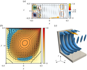


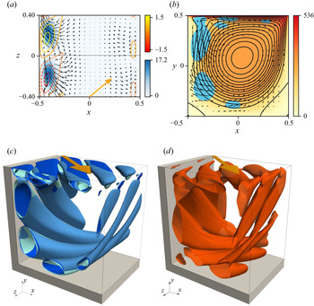


 Open access