


1. Introduction
How a stratified body of fluid responds to external forcing depends on the geometry of the container, the boundary conditions and the nature of the forcing. While much insight has been gleaned from considering plane waves in unbounded stratified domains (Staquet & Sommeria Reference Staquet and Sommeria2002; Dauxois et al. Reference Dauxois, Joubaud, Odier and Venaille2018), physical observations necessarily involve flows in finite containers. Even small amplitude forcings can lead to large responses in confined systems with strong restoring forces such as Coriolis and buoyancy. The importance of parametric forcing and resonance in geophysical and astrophysical settings is well recognized (Le Bars, Cebron & Le Gal Reference Le Bars, Cebron and Le Gal2015); the point is that small amplitude mechanical forcings do not directly drive the large-scale flows but rather convert part of the available rotational and/or potential energies into intense fluid motions by resonating inertial and/or internal modes.
A classical example of parametric resonance is the Faraday wave problem (Faraday Reference Faraday1831), where standing waves on the surface of a liquid layer in a vertically oscillating container are formed. In the Faraday wave setting the parametric forcing is the oscillatory vertical acceleration of the container resulting in a vertically modulated gravity; typically a two-layer system is studied. The response to the parametric forcing manifests as surface or interfacial waves between the two layers of different density fluids, which may be immiscible or miscible. The experiments of Benielli & Sommeria (Reference Benielli and Sommeria1998) explored vertical parametric forcing in a rectangular container, both with a two-layer system whose response was well described in terms of a system of Mathieu equations, and a continuously stratified fluid. The Mathieu equation describing a linear oscillator subject to parametric forcing is central to understanding Faraday waves (Benjamin & Ursell Reference Benjamin and Ursell1954; Miles & Henderson Reference Miles and Henderson1990; Kumar & Tuckerman Reference Kumar and Tuckerman1994). In the continuously stratified case there was some correspondence with the two-layer responses, but not all. In the two-layer system they were able to experimentally identify the resonance tongues, whereas in the continuously stratified system they were not. Using numerical Floquet analysis of a temperature stratified analog of the Benielli & Sommeria (Reference Benielli and Sommeria1998) continuously stratified experiment, the resonance tongues were clearly identified (Yalim, Lopez & Welfert Reference Yalim, Lopez and Welfert2018), and these results were used to calibrate viscous effects in a Mathieu model (Yalim, Welfert & Lopez Reference Yalim, Welfert and Lopez2019a). Nonlinear simulations showed complicated nonlinear dynamics near the edges of the resonance tongues, including subcritical behaviour to the low forcing frequency sides of the tongues (Yalim, Welfert & Lopez Reference Yalim, Welfert and Lopez2019b). Those numerical studies were in two dimensions, but Yalim, Lopez & Welfert (Reference Yalim, Lopez and Welfert2020) showed that the complex nonlinear behaviour persists in three dimensions using a container with the same spanwise aspect ratio as used experimentally in Benielli & Sommeria (Reference Benielli and Sommeria1998), until the forcing amplitude exceeded a level at which wave breaking ensues.
In Benielli & Sommeria (Reference Benielli and Sommeria1998) the forced responses to vertical oscillations of the linearly stratified rectangular container correspond to resonantly excited modes of the container. When paddles or plungers are used to force such a rectangular container (e.g. Thorpe Reference Thorpe1968; McEwan Reference McEwan1971), the response flow is a mix of modes with high regularity and beams with less regularity. More recent explorations have used increasingly more sophisticated semi-localized wave-makers to drive localized wavebeams (e.g. Mercier et al. Reference Mercier, Martinand, Mathur, Gostiaux, Peacock and Dauxois2010; Boury, Peacock & Odier Reference Boury, Peacock and Odier2019). These types of forcings inherently also include a component that is orthogonal to the direction of gravity. If the orthogonal component is small compared with the vertical accelerations then the response is largely that due to the vertical forcing, and remains well described by Mathieu equation models. On the other hand, there have been a number of studies where the parametric forcing is solely orthogonal to gravity, for the most part involving containers with a two-layer system oscillating horizontally (Wolf Reference Wolf1969, Reference Wolf1970; Wunenburger et al. Reference Wunenburger, Evesque, Chabot, Garrabos, Fauve and Beysens1999; Talib, Jalikop & Juel Reference Talib, Jalikop and Juel2007; Jalikop & Juel Reference Jalikop and Juel2009; Gaponenko et al. Reference Gaponenko, Torregrosa, Yasnou, Mialdun and Shevtsova2015; Shevtsova et al. Reference Shevtsova, Gaponenko, Yasnou, Mialdun and Nepomnyashchy2016; Gréa & Briard Reference Gréa and Briard2019; Richter & Bestehorn Reference Richter and Bestehorn2019). In these horizontally oscillating systems a peculiar feature of the responses for some forcing frequencies is the saw-tooth shape of the surface, which remains invariant in the frame of the container, and is referred to as a frozen wave.
The vertically forced rectangular container with linear stable stratification has an equilibrium solution consisting of static fluid relative to the oscillating container. It is an equilibrium solution of the full nonlinear viscous problem for any forcing amplitude and frequency. The linearization of the governing equations about this state leads to a homogeneous Mathieu system describing deviations from this state, in which gravity modulation appears parametrically (i.e. multiplicatively). The trivial solution of the Mathieu system, consisting of zero perturbation velocity and zero temperature deviation away from linear stratification, is a solution for any forcing amplitude and frequency. The existence of non-trivial solutions in the Mathieu model determine a stability boundary in amplitude/frequency space (the edges of resonance tongues) where the trivial state becomes unstable. The instabilities correspond to resonantly excited eigenmodes of the unforced stratified cavity (Thorpe Reference Thorpe1968). These resonant responses may be either synchronous or subharmonic with respect to the forcing.
In contrast, for the horizontally forced system, the static linearly stratified state is not a solution for any non-zero forcing amplitude, and so a Floquet analysis about that state is inappropriate. Instead, in the viscous nonlinear setting one needs to find the non-trivial responses at each point in parameter space. In the inviscid limit a perturbation analysis of the static linearly stratified state, using the small forcing amplitude as the perturbation variable, results at first order in a non-homogeneous linear system, where the gravity modulation appears as an external body force (i.e. additively). A similar perturbation analysis of the vertically forced system would lead to a trivial response at any order because the resulting effective gravity is a gradient term and simply modifies the pressure. The nature of the non-trivial response for the horizontally forced system depends on whether the frequency of the forcing is resonant or not. This can be codified in terms of the Fredholm alternative (Keller & Ting Reference Keller and Ting1966), conveniently described in the context of finite-dimensional differential systems (Hale Reference Hale2009): either the response is uniquely determined by the forcing, or it is resonant.
Responses obtained in stratified systems at the onset of instabilities also have strong similarities with those arising in rotating systems. In both cases, the linear inviscid limit leads to a Poincaré equation, a linear hyperbolic equation, for a perturbed temperature field (in the stratified case) or pressure field (in the rotating case). For confined systems, boundary conditions may lead to ill-posedness and a decrease in the regularity of solutions. Smooth solutions do exist and have been found via separation of variables in some geometries, such as a cylinder or a sphere in rotating systems (Kelvin Reference Kelvin1880; Greenspan Reference Greenspan1965) and in rectangular containers in stratified systems (Thorpe Reference Thorpe1968; Turner Reference Turner1979). Smooth intrinsic modes which are not completely separable have also been found, for example, in rotating rectangular containers (Maas Reference Maas2003; Wu, Welfert & Lopez Reference Wu, Welfert and Lopez2018b). However, one should in general expect singular (non-smooth) solutions (Aldridge Reference Aldridge1975; Maas & Lam Reference Maas and Lam1995; Rieutord, Georgeot & Valdettaro Reference Rieutord, Georgeot and Valdettaro2000; Harlander & Maas Reference Harlander and Maas2007; Swart et al. Reference Swart, Sleijpen, Maas and Brandts2007; Bajars, Frank & Maas Reference Bajars, Frank and Maas2013; Borcia, Abouzar & Harlander Reference Borcia, Abouzar and Harlander2014; Pillet et al. Reference Pillet, Ermanyuk, Maas, Sibgatullin and Dauxois2018; Rieutord & Valdettaro Reference Rieutord and Valdettaro2018; Wu, Welfert & Lopez Reference Wu, Welfert and Lopez2020). These non-smooth solutions, which can be described as the superposition of an infinite number of regular ‘modes’ (and as such are non-separable), have been found in the inviscid limit in geometries where some or all of the container boundaries are neither parallel nor orthogonal to gravity or the mean rotation.
In continuously stratified systems viscosity can be quantified non-dimensionally in terms of a buoyancy number  $R_N$, which is the ratio of the viscous time scale and buoyancy time scale. For small viscosity (large
  $R_N$) and small forcing amplitudes, the responses to horizontal oscillations at forcing frequencies (normalized by the buoyancy frequency) corresponding to ratios
  $r=n/m$, with
  $m$ and
  $n$ both odd integers, have mean enstrophy several orders of magnitude larger than at any other frequency (corresponding to either irrational
  $r$ or rational
  $r=n/m$ with
  $m$ and
  $n$ not both odd integers). The corresponding flow structure bears some resemblance to the eigenmodes of the unforced system at those frequencies, except that rather than being smooth, as was the case with the vertical forcing, the vorticity tends to be piecewise linear. The eigenmodes of the unforced system corresponding to frequencies associated to
  $r=n/m$ with
  $m$ and
  $n$ both odd integers are the only eigenmodes with spatio-temporal symmetry consistent with the horizontal forcing. At frequencies associated to
  $r=n/m$ with
  $m$ and
  $n$ having opposite parities, the response flows are not resonant and they tend to have piecewise constant vorticity as
  $R_N$ is increased, with the constant regions delineated by the characteristics of the linear inviscid system emanating from the corners of the container. In contrast, the vertically forced flows are resonant at these frequencies. Other horizontal forcing frequencies result in response flows with further complications, including fractal patterns. By considering infinitesimal standing wave perturbations of the static linearly stratified state, we are able to solve the resulting non-homogeneous linear system analytically in the inviscid limit (
 $R_N\to \infty$) and recover virtually all the details of the nonlinear viscous response flows computed from the Navier–Stokes–Boussinesq equations with small viscosity (large, but finite
  $R_N$) and small forcing amplitudes. At the core of the analytic solution process lies a set of functional conditions obtained by imposing the symmetry and boundary conditions.
In this paper we consider the linearly stratified square container subjected to horizontal oscillations. The body force has a constant vertical component and an oscillatory horizontal component. In § 2 the details of the problem and the governing equations are defined, their spatio-temporal symmetries are described, as is the numerical technique used for the nonlinear viscous problem. Section 3 describes these nonlinear viscous response flows at small forcing amplitudes and forcing frequencies covering the entire spectrum of the unforced system. As viscous effects are reduced (by increasing  $R_N$), the response flows tend to have lower regularity with either piecewise constant or linear vorticity. These viscous nonlinear results are reconciled by considering the linear inviscid limit. This leads to a Poincaré equation for the temperature deviation. In § 4 synchronous standing wave solutions to the Poincaré equation are found by exploiting the symmetries of the contained system. Several technical details pertaining to the analysis are presented in appendices. Section 5 provides a head-to-head comparison between the linear inviscid solutions and the nonlinear response flows at large but finite
  $R_N$ and small forcing amplitudes. Finally, § 6 summarizes and discusses potential implications for other forcing protocols, in particular, larger amplitude forcings, and the persistence of the results in three-dimensional (3-D) containers.
2. Governing equations, symmetries and numerics
Consider a fluid of kinematic viscosity  $\nu$, thermal diffusivity
  $\kappa$ and coefficient of volume expansion
  $\beta$ contained in a square cavity of side lengths
  $L$. The two vertical walls of the cavity are insulated and the two horizontal walls are held at fixed temperatures
  $T_{hot}$ at the top and
  $T_{cold}$ at the bottom, such that
  $\Delta T=T_{hot}-T_{cold}>0$. Gravity
  $g$ acts in the downward vertical direction. In the absence of any other external force, the fluid is linearly stratified. The non-dimensional temperature is
  $T=(T^*-T_{cold})/\Delta T-0.5$, where
  $T^*$ is the dimensional temperature. Length is scaled by
  $L$ and time by
  $1/N$, where
 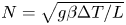 $N=\sqrt {g\beta \Delta T/L}$ is the buoyancy frequency. A Cartesian coordinate system
  $\boldsymbol {x}=(x,z)\in [-0.5,0.5]\times [-0.5,0.5]$ is attached to the cavity with its origin at the centre and the directions
  $x$ and
  $z$ aligned with the sides.
The cavity is subjected to small harmonic horizontal oscillations of non-dimensional forcing frequency and amplitude  $\omega$ and
  $\alpha$. In the cavity reference frame the non-dimensional velocity is
  $\boldsymbol {u}=(u,w)$. The boundary conditions are no-slip on all walls for the velocity
  $\boldsymbol {u}=\boldsymbol {0}$. For the temperature,
  $T=\pm 0.5$ on the conducting walls at
  $z=\pm 0.5$ and
  $\partial _x T=0$ on the insulated walls at
  $x={\pm }0.5$. Figure 1 shows a schematic of the system.

Figure 1. Schematic of the stably stratified square cavity under harmonic horizontal forcing, together with the effective gravity vector  $\boldsymbol {g}_{eff}$ relative to the horizontally oscillating cavity. A snapshot of the vorticity
  $\eta$ is shown corresponding to buoyancy number
  $R_N=10^6$, Prandtl number
  ${Pr}=1$, forcing frequency
  $\omega =0.71$ and forcing amplitude
 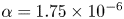 $\alpha =1.75 \times 10^{-6}$.
Under the Boussinesq approximation, the non-dimensional governing equations are
 \begin{equation} \left. \begin{gathered} \partial_t u + u\partial_x u+w\partial_z u ={-}\partial_x p + \frac{1}{R_N}\nabla^2 u + \alpha T\sin\omega t,\\ \partial_t w + u\partial_x w+w\partial_z w ={-}\partial_z p + \frac{1}{R_N}\nabla^2 w + T,\\ \partial_t T + u\partial_x T+w\partial_z T = \frac{1}{{Pr}R_N}\nabla^2 T, \\ \partial_x u + \partial_z w = 0, \end{gathered} \right\} \end{equation}
where  $p$ is the pressure,
  ${Pr} = \nu /\kappa$ is the Prandtl number and the buoyancy number
 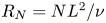 $R_N = NL^2/\nu$ is the ratio of the viscous and buoyancy time scales (it is the square root of the Grashof number). The buoyancy number
  $R_N$ can also be viewed as a ratio of a Reynolds number
  $u'L/\nu$ and Froude number
  $u'/NL$, where
  $u'$ is a characteristic velocity, i.e.
  $(u'L/\nu )/(u'/NL)=NL^2/\nu =R_N$ (Riley & Lelong Reference Riley and Lelong2000). For the most part, we shall report on the temperature deviation,
  $\theta =T-z$, rather than on
  $T$ itself.
For linearly stratified fluid in a rectangular container, if the boundary conditions on the horizontal walls for the stratifying agent are of Dirichlet type, such as is the case for fixed temperature on those walls, then the static linearly stratified state is a stable equilibrium irrespective of the viscosity or the thermal diffusivity of the fluid. This is not the case for salt stratification as the appropriate horizontal wall boundary conditions are of Neumann type, corresponding to no salt flux through the walls. The equilibrium state in that case is static with uniform density. In the inviscid limit the static linearly stratified equilibrium state with Dirichlet horizontal wall boundary conditions has neutral (i.e. zero growth rate) modes with a dense but discrete spectrum, consisting of a set of intrinsic frequencies (eigenvalues) which, when normalized by the buoyancy frequency, are in the interval  $0<|\sigma _r|<1$. Finite viscosity imparts negative growth rates to these modes, so that in order to have a sustained non-trivial response flow, a physical viscous system needs to be continuously forced. The values of
  $r$ for the intrinsic modes depend on the aspect ratio of the rectangular container. In the case of the square studied here, the discrete set corresponds to rationals
  $r=n/m$. The slopes of the characteristics are
  ${\pm }r$. If
  $r$ is rational the characteristics retrace, whereas if
  $r$ is irrational the characteristics never retrace and are said to be ergodic.
The static linearly stratified state 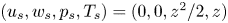 $(u_s, w_s, p_s, T_s)=(0, 0, z^2/2, z)$ is a solution of the unforced system, (2.1) with
  $\alpha =0$, for any
  ${Pr}$ and
  $R_N$. When subjected to horizontal oscillations of small amplitude
  $\alpha$, the response is synchronous with the forcing at frequency
  $\omega$ and has discrete time translation invariance
 \begin{equation} \mathcal{T}:[u,w,p,\theta](x,z,t)\mapsto[u,w,p,\theta](x,z,t+\tau), \end{equation}
where  $\tau =2{\rm \pi} /\omega$ is the forcing period. The system is also invariant to two half-period-flip space–time symmetries
  $\mathcal {H}_x$ and
  $\mathcal {H}_z$, whose actions are
 \begin{gather} \mathcal{H}_x:[u,w,p,\theta](x,z,t)\mapsto[{-}u,w,p,\theta]({-}x,z,t+\tau/2), \end{gather}
 \begin{gather}\mathcal{H}_z:[u,w,p,\theta](x,z,t)\mapsto[u,-w,p,-\theta](x,-z,t-\tau/2). \end{gather}
The two symmetries  $\mathcal {H}_x$ and
  $\mathcal {H}_z$ combine into a centrosymmetry
 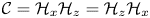 $\mathcal {C}=\mathcal {H}_x\mathcal {H}_z=\mathcal {H}_z\mathcal {H}_x$, corresponding to a reflection through the origin, whose action is
 \begin{equation} \mathcal{C}:[u,w,p,\theta](x,z,t)\mapsto[{-}u,-w,p,-\theta]({-}x,-z,t). \end{equation}
 The governing equations are solved numerically using a spectral-collocation method. It is the same technique as was used in Wu, Welfert & Lopez (Reference Wu, Welfert and Lopez2018a), Yalim et al. (Reference Yalim, Welfert and Lopez2019b), Grayer et al. (Reference Grayer, Yalim, Welfert and Lopez2020) and Yalim et al. (Reference Yalim, Lopez and Welfert2020). Briefly, the velocity, pressure and temperature are approximated by polynomials of degree  $n=160$ for
  $R_N\le 10^6$ and
  $n=224$ for
  $R_N=10^7$, associated with the Chebyshev–Gauss–Lobatto grid. A selection of results were ‘spot tested’ using
  $n=600$ for
  $R_N=10^7$ in order to confirm that the results using
  $n=224$ are indeed converged. A fractional step improved projection method, based on a linearly implicit and stiffly stable second-order accurate scheme, is used to integrate in time with
  $315/\omega$ time steps (rounded to the nearest decade) per forcing period, corresponding to a target time step
  $\delta t=2\times 10^{-2}$. Here, we fix
  ${Pr}=1$ and the forcing amplitude
  $\alpha =1.75\times 10^{-6}$, and consider variations in
  $R_N$ and
  $\omega$. The choice of small
  $\alpha$ is such that for the range of
  $R_N$ considered, the response flow remains the primary response, invariant to the spatio-temporal symmetries
  $\mathcal {H}_x$ and
  $\mathcal {H}_z$.
3. Limit cycle responses to small amplitude forcing
We begin by broadly describing how the flow responds over a wide range of squared forcing frequencies,  $0<\omega ^2<1$, covering the spectrum of the intrinsic modes, for several
  $R_N\in [10^2, 10^7]$. Figure 2
 $(a)$ summarizes these results in terms of a Bode magnitude plot consisting of response curves using the time-averaged enstrophy in the container,
  $\langle \mathcal {E}\rangle _\tau$, as a measure of the relative strength of the response flow, where
 \begin{equation} \langle\mathcal{E}\rangle_\tau= \frac{1}{\tau}\int_{0}^{\tau} \int_{{-}0.5}^{\;0.5}\int_{{-}0.5}^{\;0.5} \eta^2 \textrm{d}\kern0.06em x\, \textrm{d}z\, \textrm{d}t, \end{equation}
 $\eta =\partial _z u -\partial _x w$ is the vorticity and
  $\tau =2{\rm \pi} /\omega$ is the forcing period, and figure 2
 $(b)$ for the phase lag
  $\varphi$ between phases associated with maximal horizontal forcing and maximal vorticity at the centre of the cavity in the response flow. The results are presented in terms of
  $\omega ^2$ rather than
  $\omega$ as the responses have a certain symmetry around
  $\omega ^2=1/2$, which is detailed below. For the parameter ranges considered, all response flows are centrosymmetric limit cycles synchronous with the horizontal forcing.

Figure 2. Bode plot, consisting of  $(a)$ magnitude response curves,
  $\langle \mathcal {E}\rangle _\tau$ vs.
  $\omega ^2$, and
  $(b)$ phase lag response curves,
  $\varphi$ vs.
  $\omega ^2$, for
  $R_N$ as indicated. The rational values indicated are the ratios
  $r=n/m$ at squared frequencies
  $\omega ^2=1/(1+r^2)$.
Focusing on the squared forcing frequency range  $0.45<\omega ^2<0.55$, which brackets the squared frequency
  $\omega ^2=m^2/(m^2+n^2)=1/2$ corresponding to the frequency of the primary intrinsic inviscid eigenmode with horizontal and vertical half-wavenumbers
  $m=n=1$, the response is similar to that of a damped oscillator forced near its natural frequency. The magnitude and phase lag responses are almost flat at large damping (e.g. the
  $R_N=10^2$ responses), and as
  $R_N$ is increased, the magnitude response begins to show a broad increase preferentially near but below
  $\omega ^2=1/2$, which sharpens and whose peak converges towards
  $\omega ^2=1/2$ with increasing
  $R_N$. The phase lag response has an inflection point at the frequencies where the magnitude response has its peak, converging toward a step-function response as
  $R_N$ is increased. The phase lag
  $\varphi \to 90^{\circ }$ at
  $\omega ^2=1/2$,
  $\varphi \to 0^{\circ }$ for
  $\omega ^2<1/2$, and
  $\varphi \to 180^{\circ }$ for
  $\omega ^2>1/2$. If the system were a simple damped spring–mass with a single natural frequency, this is all that would happen for forcing amplitudes that are not too large, but the unforced stratified cavity has natural frequencies
  $\sigma _r=m/\sqrt {m^2+n^2}=1/\sqrt {1+r^2}$ for all rational values of
  $r=n/m$ (Thorpe Reference Thorpe1968). For
  $R_N\le 10^3$, all resonances are damped except for the
  $r=1/1$ resonance just described. At
  $R_N=10^4$, the magnitude response shows the development of peaks at frequencies corresponding to
  $r=3/1$ and
  $r=1/3$, as well as a weaker
  $r=5/1$ peak. These, together with the
  $r=1/5$ peak, sharpen with increasing
  $R_N$, much like the
  $r=1/1$ peak. The phase lag behaviour is consistent with traversing through resonances, with the
  $\varphi$ response curve developing inflection points near the resonating natural frequencies which develop into step functions as
  $R_N$ is increased, with the step in
  $\varphi$ being
  $180^{\circ }$ across each resonance. As
  $R_N$ is increased, more resonances are less damped and additional peaks become evident in the magnitude and phase lag responses. At
  $R_N=10^7$, these peaks are identified in figure 2
 $(a)$ by the rationals
  $r=n/m$, and the phase lag response only has inflections at these frequencies. If
  $R_N$ is not sufficiently large for a particular resonance, there may only be a very slight peak in the magnitude response and the phase response does not change by
  $180^{\circ }$ across the resonance but instead changes slightly and returns back to the phase lag on the other side of the resonance. Only the rationals
  $r=n/m$ with
  $m$ and
  $n$ both odd integers are resonated. These correspond to intrinsic modes whose spatio-temporal symmetries are compatible with those of the horizontal forcing,
  $\mathcal {H}_x$ and
  $\mathcal {H}_z$.
Figures 3 and 4 show snapshots of  $\eta$ and
  $\theta$ for various
  $\omega$ and
  $R_N$ at phases of the forcing where
  $\eta$ at the origin and
  $\theta$ are maximal (note that the maxima in
  $\eta$ and
  $\theta$ are a quarter period out of phase). The supplementary movies 1 and 2 (available at https://doi.org/10.1017/jfm.2021.73) show animations of these over one forcing period. All cases shown in the movies are synchronous with the horizontal forcing, so that the phase lags for each case are easy to visualize.

Figure 3. Snapshots of the vorticity  $\eta$ at indicated
  $\omega ^2$ and
  $R_N$, at times when
  $\eta$ at the origin is maximal. The supplementary movie 1 animates these response flows over one forcing period.

Figure 4. Snapshots of the temperature deviation  $\theta$ at indicated
  $\omega ^2$ and
  $R_N$, at times corresponding to a quarter period after
  $\eta$ is maximal at the origin. The supplementary movie 2 animates these response flows over one forcing period.
When  $R_N$ is small, such as
  $R_N=10^2$, the response flow across the whole frequency range is a single-cell limit cycle, somewhat reminiscent of the 1:1 intrinsic eigenmode with squared eigenfrequency
  $\sigma _{1}^2=0.5$. As
  $R_N$ is increased, the response flow tends to appear less smooth with either piecewise constant or piecewise linear vorticity, depending on the forcing frequency. For example, for
 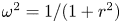 $\omega ^2=1/(1+r^2)$ with
  $r=1/1$,
  $1/3$ and
  $3/1$ (i.e.
  $\omega ^2=0.5$, 0.9 and 0.1), the vorticity of the response flows consists of one cell or three cells lined up either vertically or horizontally, with piecewise linear segments delimited by lines that start and end at the four corners of the cavity, reflecting a finite number of times on the walls, and whose slopes
  ${\pm }r$ correspond to the characteristics of the linear inviscid problem. For
  $\omega ^2=0.8$ and 0.2, corresponding to
  $r=1/2$ and
  $r=2/1$, the response vorticity is piecewise constant with the pieces again being delimited by lines starting and ending at the four corners with slopes
  ${\pm }r$. The supplementary movies 1 and 2 show that for these rational values of
  $r$, the response flows are standing waves. For
  $\omega ^2=0.3$ and 0.7, the corresponding
  $r=\sqrt {7/3}$ and
  $\sqrt {3/7}$ are irrational and inviscid characteristic lines starting from corners do not return to corners after a finite number of reflections, although they may get arbitrarily close to the corners. Even at
  $R_N=10^7$, viscous dissipation and detuning effects are still present. For other irrational values of
  $r$, such as
  $\omega ^2=0.3$ with
  $r=\sqrt {7/3}$ and
  $\omega ^2=0.6$ with
  $r=\sqrt {2/3}$, the limit cycle response is not a standing wave. From the vorticity response, it appears that the flow at
  $\omega ^2$ corresponds to that at
  $1-\omega ^2$ with the vertical and horizontal directions interchanged, but this is not the case for the temperature deviation response.
Figure 5 provides a further quantitative demonstration of the piecewise low-degree polynomial (spline) nature of the vorticity and temperature deviation. It shows the profiles at  $z=0$ of the
  $\omega ^2\ge 0.5$ responses for the four largest values of
  $R_N$ used. Several observations are in order: (i) the vorticity (shown in figure 5a,c,e,g,i), being a derived quantity obtained from the velocity components
  $u$ and
  $w$, is in general less regular than the temperature deviation (shown in figure 5b,d,f,h,j); (ii) for
  $\omega ^2=0.8$, both the vorticity and temperature profiles scale with the forcing amplitude
  $\alpha ^{-1}$ and converge with increasing
  $R_N$ towards piecewise constant and linear functions of the horizontal coordinate
  $x$, respectively; (iii) for
  $\omega ^2=0.5$ or
  $0.9$, corresponding to peaks in the response diagram (figure 2), the convergence with
  $R_N$ requires additional scaling with a factor
  $R_N^{-0.5}$; (iv) for
  $\omega ^2=0.7$, the vorticity profile exhibits oscillations in the vicinity of the ‘jumps’, and the temperature deviation also has oscillations at those locations; (v) for
  $\omega ^2=0.6$, new features appear with increasing
  $R_N$, with large oscillations in the vorticity profile as well as noticeable oscillations in the temperature deviation profile.
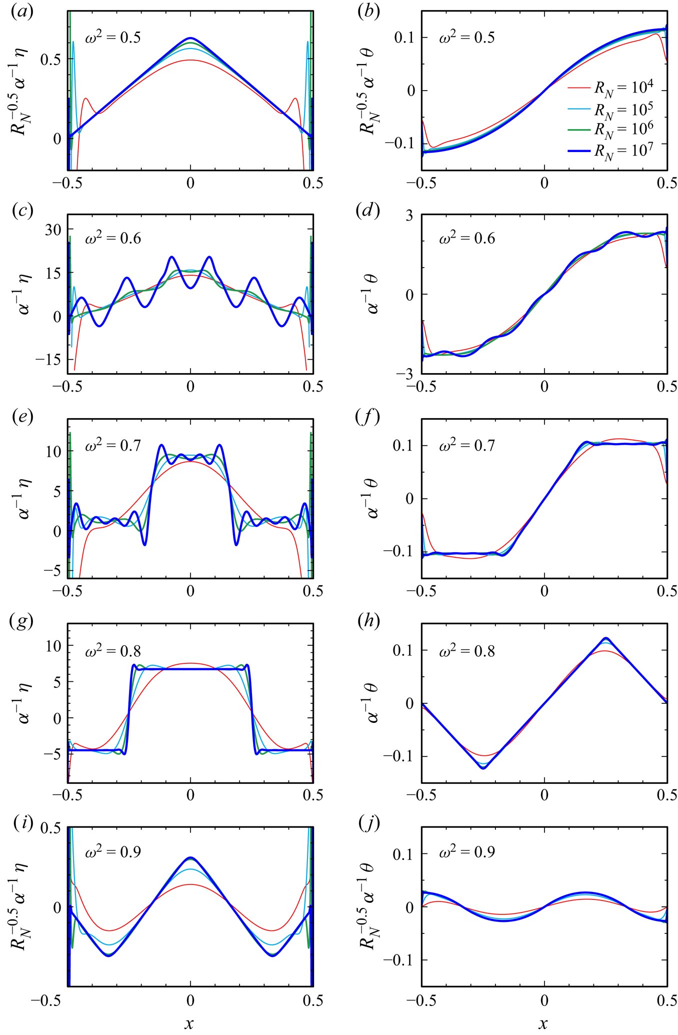


While the jumps in the  $\omega ^2=0.7$ case are reminiscent of artifacts due to the Gibbs phenomenon in the spectral approximation of discontinuous functions (Tadmor Reference Tadmor2007), the sheer size of the oscillations cannot be solely accounted for by such effects, which are known to be limited to approximately
  $9\,\%$ of the jump at a discontinuity. Increasing the numerical resolution does not change these profiles (at the respective values of
  $R_N$). This is contrary to what is expected of Gibbs oscillations, which become more localized with increased resolution, due to pointwise convergence away from jumps. The inviscid analysis carried out in the next section reconciles all the nonlinear viscous responses at large
  $R_N$ and sheds light on the above observations, in particular, the general low regularity of solutions and the property that, in this problem, the response flows seem to exhibit finer-scale features at certain forcing frequencies when viscous effects are reduced.
4. Weak responses in the inviscid limit
The responses to horizontal forcing appear to be standing waves with less regularity than those observed in the case of purely vertical oscillatory forcing studied in Yalim et al. (Reference Yalim, Lopez and Welfert2018). Here, we show how the responses to horizontal forcing can be constructed in the inviscid limit via a first-order perturbation analysis of the static linearly stratified state, using the forcing amplitude  $\alpha$ as the small parameter. Specifically, in the inviscid limit (
 $R_N\to \infty$), using
  $\alpha$ as the small perturbation parameter and neglecting terms of order
  $\alpha ^2$ and higher, the equations describing the evolution of deviations
  $(u,w,p,\theta )$ away from
  $(u_s,w_s,p_s,T_s)$ are
 \begin{equation} \left. \begin{gathered} \partial_t u ={-}\partial_x p + z\alpha\sin\omega t,\\ \partial_t w ={-}\partial_z p + \theta,\\ \partial_t \theta ={-}w,\\ \partial_x u + \partial_z w = 0, \end{gathered} \right\} \end{equation}
subject to Dirichlet boundary conditions  $u({\pm }0.5,z) = w(x,{\pm }0.5) = \theta (x,{\pm }0.5) = 0$. Note that the term
  $z\alpha \sin \omega t$ appearing in (4.1) cannot be absorbed into the pressure gradient in the form of a modified pressure. This results in a non-homogeneous (forced) linear system (4.1), whose general solution consists of the general solution to the homogeneous (unforced,
  $\alpha =0$) system plus a particular solution. For
  $\omega ^2\ne 1$, a particular solution is
 \begin{equation} \begin{bmatrix}u_p\\ w_p\end{bmatrix} =\dfrac{\alpha}{1-\omega^2}\begin{bmatrix}0\\ -x\omega\end{bmatrix}\cos\omega t,\quad \begin{bmatrix}p_p\\ \theta_p\end{bmatrix} =\dfrac{\alpha}{1-\omega^2}\begin{bmatrix}xz(1-\omega^2)\\ x\end{bmatrix}\sin\omega t. \end{equation}
Eliminating  $u$,
$u$,  $w$ and
  $p$ from (4.1) leads to the Poincaré equation (Poincaré Reference Poincaré1885)
 \begin{equation} \partial_{tt} (\partial_{xx} +\partial_{zz}) \theta +\partial_{xx} \theta=0, \end{equation}
which is independent of the forcing amplitude  $\alpha$.
We now consider synchronous standing wave solutions of the form
 \begin{equation} \theta_h=[\,f(x+rz)+g(x-rz)]\sin\sigma_rt, \end{equation}
with arbitrary waveform functions  $f$ and
  $g$ (that may depend on
  $r>0$) and frequency
  $\sigma _r$ satisfying the dispersion relation
 \begin{equation} \sigma_r^2=1/(1+r^2) \quad\text{with}\ 0<\sigma_r^2<1. \end{equation}
Note that the waveform functions  $f$ and
  $g$ need only be defined for arguments in the interval
  $[-(1+r)/2,(1+r)/2]$.
Solutions to the homogeneous system are obtained by substituting (4.4) into (4.1) and setting  $\alpha =0$, i.e.
 \begin{equation} \left. \begin{gathered} \begin{bmatrix}u_h\\w_h\end{bmatrix} =\begin{bmatrix}r\sigma_r[\,f(x+rz)-g(x-rz)]\\ -\sigma_r[\,f(x+rz)+g(x-rz)]\end{bmatrix} \cos\sigma_rt,\\ \begin{bmatrix}p_h\\\theta_h\end{bmatrix} =\begin{bmatrix}\lambda_r[F(x+rz)-G(x-rz)] \\ f(x+rz)+g(x-rz)\end{bmatrix} \sin\sigma_rt, \end{gathered} \right\} \end{equation}
where 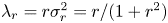 $\lambda _r=r\sigma ^2_r=r/(1+r^2)$,
  $F^\prime =f$,
  $G^\prime =g$ and
  $(\cdot )^\prime$ denotes differentiation with respect to the argument. The system (4.1) forced at frequency
  $\omega =\sigma _r$ thus admits synchronous responses
 \begin{equation} \left. \begin{gathered} \begin{bmatrix}u\\w\end{bmatrix} =\begin{bmatrix}u_p+cu_h\\w_p+cw_h\end{bmatrix} =\begin{bmatrix}cr\sigma_r[\,f(x+rz)-g(x-rz)]\\ -\alpha x/(r^2\sigma_r)-c\sigma_r[\,f(x+rz)+g(x-rz)]\end{bmatrix} \cos\sigma_rt, \\ \begin{bmatrix}p\\\theta\end{bmatrix} =\begin{bmatrix}p_p+cp_h\\\theta_p+c\theta_h\end{bmatrix} =\begin{bmatrix} \alpha xz+c\lambda_r[F(x+rz)-G(x-rz)]\\ \alpha x/(r^2\sigma_r^2)+c[\,f(x+rz)+g(x-rz)] \end{bmatrix} \sin\sigma_rt, \end{gathered} \right\} \end{equation}
for any constant  $c$, where the identity
  $1/(1-\omega ^2)=1/(1-\sigma _r^2)=1/(r^2\sigma _r^2)$ has been used. The streamfunction
  $\psi$, whose gradient is
  $(\partial _x \psi ,\partial _z \psi )=(-w,u)$, and the vorticity
  $\eta =\partial _z u-\partial _x w$ of these responses are
 \begin{equation} \begin{bmatrix}\psi\\\eta\end{bmatrix}= \begin{bmatrix} \alpha x^2/(2r^2\sigma_r)+c\sigma_r[F(x+rz)+G(x-rz)]\\ \alpha/(r^2\sigma_r)+(c/\sigma_r)[\,f'(x+rz)+g'(x-rz)] \end{bmatrix}\cos\sigma_rt. \end{equation}
The linear system (4.1) has the same spatio-temporal symmetries,  $\mathcal {H}_x$ and
  $\mathcal {H}_z$, as the full Navier–Stokes system (2.1). For
  $c\ne 0$, these symmetries imply, for all
  $|x|\le 0.5$ and
  $|z|\le 0.5$ (i.e. everywhere inside the container), that
 \begin{gather} f({\mp} x\pm rz)-g({\mp} x\mp rz)={\pm} f(x+rz)\mp g(x-rz), \end{gather}
 \begin{gather}f({\mp} x\pm rz)+g({\mp} x\mp rz)={\mp} f(x+rz)\mp g(x-rz). \end{gather}
Adding (4.9a) and (4.9b) shows that  $f=g$ and that both waveform functions are odd. The resulting
  $u$ in (4.7) is even in
  $x$ and odd in
  $z$,
$z$,  $w$ and
  $\theta$ are odd in
  $x$ and even in
  $z$, while
  $p$ is odd in both
  $x$ and
  $z$, and
  $\psi$ and
  $\eta$ are both even in
  $x$ and
  $z$.
$z$.
In general, the imposition of boundary conditions on the Poincaré equation (4.3) leads to ill-posedness, with no solution when it is overspecified or multiple solutions if it is underspecified. The condition  $u(0.5,z,t)=0$ constraints
  $f$ to be even around
  $0.5$,
 \begin{equation} f(0.5+\zeta)=f(0.5-\zeta), \quad\text{where}\ |\zeta|\le r/2\ \text{and}\ \zeta=rz, \end{equation}
while the boundary condition  $w(x,0.5,t)=0$ requires
 \begin{equation} f(x+r/2)+f(x-r/2)={-}\alpha x/(cr^2\sigma_r^2), \quad |x|\le 0.5. \end{equation}
The following Fredholm alternative then holds for the waveform function  $f$:
$f$:
A1: either
 $c=c_r=-\alpha /(2r^2\sigma _r^2)=-\alpha /(2r\lambda _r)$ is finite and $f$ satisfies the functional equation
(4.12)\begin{equation} f(x+r/2)+f(x-r/2)=2x, \quad |x|\le0.5; \end{equation}
$c=c_r=-\alpha /(2r^2\sigma _r^2)=-\alpha /(2r\lambda _r)$ is finite and $f$ satisfies the functional equation
(4.12)\begin{equation} f(x+r/2)+f(x-r/2)=2x, \quad |x|\le0.5; \end{equation}A2: or,
$c=\infty$ and $f$ is even around $r/2$,
(4.13)\begin{equation} f(r/2+x)={-}f(x-r/2)=f(r/2-x), \quad |x|\le0.5. \end{equation}


The Fredholm alternative is a classical tool describing the existence of solutions of non-homogeneous linear equations; see Hale (Reference Hale2009) for a description in the differential equations context. Here, the alternative A2 is similar to case (A) in theorem 3 of Swart et al. (Reference Swart, Sleijpen, Maas and Brandts2007), corresponding to multiple solutions defined up to a scaling factor. The three conditions, (4.10),  $f$ odd, and either of (4.12) or (4.13), form systems of functional equations of the Schröder or Abel type (Kuczma, Choczewski & Ger (Reference Kuczma, Choczewski and Ger1990), § 3.5). The relevance of these types of equations to confined stratified flows was originally recognized by Manton & Mysak (Reference Manton and Mysak1971), and later exploited by Beckebanze (Reference Beckebanze2015) and Beckebanze & Keady (Reference Beckebanze and Keady2016) to obtain exact inviscid solutions with low regularity properties in a stratified trapezoidal channel. One major complication in the flows presently under consideration, compared with that considered in Beckebanze (Reference Beckebanze2015), is due to the forcing term in (4.1). Although this term does not affect the Poincaré equation (4.3), it changes the type of the resulting condition, from a (non-homogeneous/forced) Abel equation (4.12) to a (homogeneous/unforced) Schröder equation (4.13).
In the remainder of this section we describe solutions that are obtained for different values of  $r$. For the square cavity considered here, the nature of the solutions depends on whether or not
  $r$ is rational, i.e. whether the characteristic lines emanating from the corners of the cavity,
  $x\pm rz=\pm 0.5(1\pm r)$, retrace or not. Furthermore, when
  $r$ is rational, the nature of the solutions depends on the parities of the integers
  $m$ and
  $n$ in the irreducible representation of
  $r=n/m$ (greatest common denominator
  $\text {gcd}(m,n)=1$). Since the waveform function
  $f$ is determined from conditions that depend on
  $r$, we shall use the notation
  $f_r$ instead of
  $f$ when referring to a specific value of
  $r$, with a resulting response flow
  $(u_r,w_r,p_r,\theta _r)$.
4.1. Alternative A1: forced responses
There is a relationship between the solutions of (4.1) at squared forcing frequency 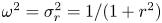 $\omega ^2=\sigma _r^2=1/(1+r^2)$, associated with waveform function
  $f_r$, and those at
  $1-\sigma _r^2=r^2/(1+r^2)=1/(1+(1/r)^2)$, associated with
  $f_{1/r}$. The details are provided in Appendix A. It is therefore sufficient to consider
  $r\in (0,1)$, i.e.
  $\sigma _r^2\in (1/2,1)$.
First, we identify waveform functions  $f_r$ satisfying (4.12) for selected rational values
  $r=n/m$ with
  $m>n$. Evaluating (4.12) at
  $\boldsymbol {x}=[x_j]_{1\le\, j\le m}$ with
  $x_j=j/(2m)$,
  $j=1,\ldots ,m$, and using the symmetries approximately
  $0$ (
$0$ ( $\,f_r$ odd) and
  $1/2$ (4.10), yields an
  $m\times m$ linear system in
  $\boldsymbol {f}_r(\boldsymbol {x})=[\,f_r(x_j)]_{1\le\, j\le m}$,
 \begin{equation} \boldsymbol{\mathsf{A}}\,\boldsymbol{f}_r(\boldsymbol{x})=2\boldsymbol{x}. \end{equation}
Harlander & Maas (Reference Harlander and Maas2007) derived a similar system using a boundary collocation approach for the solution of the Poincaré equation in two-dimensional (2-D) containers.
When  $m$ and
  $n$ have opposite parities, this system is non-singular and has a unique solution
  $\boldsymbol {f}_r(\boldsymbol {x})$. The construction of the system and its solution is illustrated in Appendix B for the case with
  $m=11$ and
  $n=4$. The linear spline obtained by connecting the points
  $[x_j,f_r(x_j)]$ satisfies (4.10) and (4.12) for all
  $x\in [-(1+r)/2,(1+r)/2]$. This solution
  $f_r$ is plotted in red in the first row of figure 6 for the cases
  $n=1$ and
  $m=2,4,6,8$ and 10. A unique 2-periodic extension, obtained by enforcing (4.10) and
  $f_r(-\zeta )=-f_r(\zeta )$ for all real
  $\zeta$, is shown in blue. This extension satisfies
  $f_r(\pm 1)=0$. Note that additional periodic extensions exist for
  $0 < r < 1$,
  $[-(1+r)/2,(1+r)/2]\subset [-1,1]$.

Figure 6. Waveform function  $f_r$ in
  $[-1.5,1.5]\times [-1.25,1.25]$ and the associated scaled forced responses
  $\eta _r$ at phase 0 and
  $\theta _r$ at phase
  ${\rm \pi} /2$, from (4.15) at
  $r$ as indicated. The blue curve is the 2-periodic extension of the red curve
  $f_r$ defined in the interval
  $[-(1+r)/2,(1+r)/2]$.
The value of the waveform function  $f_r$ in
  $[-(1+r)/2,(1+r)/2]$ completely determines the response flow of the forced linear system (4.1) everywhere in the square cavity. This response flow is
 \begin{equation} \left. \begin{gathered} \begin{bmatrix} u_r \\ w_r \end{bmatrix} =c_r\sigma_r\begin{bmatrix}r[\,f_r(x+rz)-f_r(x-rz)]\\ 2x-f_r(x+rz)-f_r(x-rz)\end{bmatrix}\cos\sigma_rt,\\ \begin{bmatrix} p_r \\ \theta_r \end{bmatrix} ={-}c_r\begin{bmatrix} \lambda_r[2r xz-F_r(x+rz)+F_r(x-rz)]\\ 2x-f_r(x+rz)-f_r(x-rz) \end{bmatrix} \sin\sigma_rt. \end{gathered} \right\} \end{equation}
Its magnitude is linearly proportional to the forcing amplitude  $\alpha$.
The forced response (4.15) is now considered for three different sequences of rationals  $r=n/m$ with
  $n$ and
  $m$ of opposite parities, which converge to
  $r=0$,
  $r=1/\sqrt {2}$ (an irrational number) and
  $r=1$. These sequences reveal qualitatively different behaviours.
The vorticity  $\eta _r$ and temperature deviation
  $\theta _r$ for the sequence
  $r=1/m$,
  $m=2,4,6,\ldots$ converging to
  $r=0$, associated with
  $\sigma _r^2=1/(1+r^2)=1$, are illustrated in figure 6 for the first five cases
  $m=2,4,6,8$ and
  $10$. For
  $r=1/2$,
  $\eta _r$ is piecewise constant with the pieces delimited by the characteristic lines emanating from the corners forming a pattern known as a harlequin print, and
  $\theta _r$ is piecewise linear in the form of two pyramids, one positive and the other negative, either side of
  $x=0$. As the even integer
  $m$ increases, the 2-periodic extension of
  $f_r$ looks more and more like a triangular wave with
  $f_r(x)=x$ for
  $|x|\le 0.5$ and the response flows consist of
  $m/2$ copies of the
  $r=1/2$ response with
  $x\to (m/2)x$.
We now consider a sequence of rationals  $r=n/m$ with
  $m$ and
  $n$ of opposite parities, converging to the irrational value
  $r=1/\sqrt {2}$, corresponding to
  $\sigma _r^2=1/(1+r^2)=2/3$. Such a sequence can be obtained from successive partial sums of the continued fraction representation
 \begin{equation} \dfrac{1}{\sqrt{2}}=\dfrac{\sqrt{2}}{2}= \dfrac{1}{2}\left[1+\dfrac{1}{2+\dfrac{1}{2+\cdots}}\right], \end{equation}
according to the iteration  $r\to (1+r)/(1+2r)$, starting with the case
  $r=1/2$. Figure 7 shows the waveform function
  $f_r$ and the associated response
  $\eta _r$ and
  $\theta _r$ for five consecutive iterates of
  $r$. The value
  $f_r(1/2)$ is observed to rapidly approximate
  $1$ as
  $r\to 1/\sqrt {2}$, with
  $f_r$ exhibiting increasingly higher frequency spatial variations, and finer and finer structure in the corresponding
  $\eta _r$ and
  $\theta _r$. The curve
  $f_{1/\sqrt {2}}$, obtained at the limit
  $r=1/\sqrt {2}$, appears to be fractal.

Figure 7. Waveform function  $f_r$ in
  $[-1.5,1.5]\times [-1.25,1.25]$ and associated scaled forced responses
  $\eta _r$ at phase 0 and
  $\theta _r$ at phase
  ${\rm \pi} /2$ for a series of rational
  $r$ values converging to the irrational
  $1/\sqrt {2}$, corresponding to
  $\sigma _r^2=2/3$. The blue curve is the 2-periodic extension of the red curve
  $f_r$ defined in the interval
  $[-(1+r)/2,(1+r)/2]$.
Figure 8 shows  $f_r$ and
  $\eta _r$ at a rational value of
  $r$ approximating
  $1/\sqrt {2}$, obtained from the fourteenth iterate of the sequence. The figures appear qualitatively similar to lower iterates shown in figure 7; the higher iterates allow us to zoom-in and explore the fractal nature of the response in the limit
  $r\to 1/\sqrt {2}$, from which the similarity relation
 \begin{equation} f_r(0.5s+[1-s]x) = s\,f_r(0.5)+[1-s]f_r(x), \end{equation}
with  $s=2r/(1+r)=2\sqrt {2}-2\approx 0.828$, can be inferred. The relation (4.17), equivalent to
 \begin{equation} \begin{bmatrix}\zeta\\\, f_r(\zeta)\end{bmatrix} =\begin{bmatrix}0.5\\ \,f_r(0.5)\end{bmatrix} +(1-s)\begin{bmatrix}x-0.5\\ \,f_r(x)-f_r(0.5) \end{bmatrix}, \end{equation}
shows that the graph of  $f_{1/\sqrt {2}}$ is invariant under the homothety with similarity factor
  $1-s=3-2\sqrt {2}\approx 0.172$ and centre
  $(0.5,f_{1/\sqrt {2}}(0.5))=(0.5,1)$. Figure 8 illustrates how the curve
  $f_{1/\sqrt {2}}$ in the range
  $[s/2, 1-s/2]$, of size
  $1-s$ centred around
  $0.5$, is a scaled-down copy of itself from the range
  $[0,1]$. The supplementary movie 3 shows a continuous zoom into the region in the neighbourhood of the point
  $(x,z)=(0.5,0)$ of the response
  $\eta _r$ shown in figure 8. The relation (4.17) is not trivial and can be verified to hold for other quadratic irrational values of
  $r$, with exactly the same definition of
  $s(r)$ when
  $r^2=1-1/m$,
  $m=3,4,\ldots$, and when
  $r^2=1+1/m$,
  $m=1,2,\ldots$, or with a modified rational relationship for other quadratic irrational values of
  $r$.
$r$.

Figure 8. Zoom-in in the neighbourhood of  $(0.5,0)$ for
  $\eta _r$ at phase 0; (a–c) waveform function
  $f_{1/\sqrt {2}}$ in windows
  $[-1.5,1.5]\times [-1.25,1.25]$ (a,d),
  $[0,1]\times [0,1]$ (b,e) and
  $[s/2, 1-s/2]\times [s, 1]$ (c, f) with
  $s=2\sqrt {2}-2$; (d–f)
  $\eta _r$ in regions
  $[-0.5, 0.5]\times [-0.5, 0.5]$ (square cavity; a,d),
  $[0, 1/2]\times [-1/4, 1/4]$ (b,e) and
  $[s/2, 1/2]\times [-(1-s)/4,(1-s)/4]$ (c,f). The supplementary movie 3 shows a continuous zoom-in of the response
  $\eta _r$ about the point
  $(x,z)=(0.5,0)$.
The third sequence of rationals considered is  $r=n/m=(m-1)/m=1-1/m$,
  $m=2,3,4,\ldots$ converging to
  $r=1$, which is associated with
  $\sigma _r^2=1/(1+r^2)=1/2$. Figure 9 illustrates the behaviour of the solution of the functional equations,
  $f_r$, and the corresponding forced response
  $\eta _r$ and
  $\theta _r$. As
  $m$ increases, the maximum value of
  $f_{1-1/m}$, which is attained at
  $0.5$, increases unboundedly as
  ${O}(m)={O}(1/(1-r))$. As a consequence, the forced response also grows in magnitude as
  $m\to \infty$ and
  $r\to 1$, with the piecewise constant vorticity
  $\eta _r$ showing a finer and finer harlequin pattern converging towards a piecewise linear vorticity profile in the shape of an inverted pyramid, and the temperature deviation
  $\theta _r$ converges towards a piecewise quadratic field with isocontours in the form of perfect (arcs of) circles centred at
  $(\pm 0.5,0)$ and hyperbolas centred at
  $(0,\pm 0.5)$ meeting at the limiting characteristics
  $x\pm z=0$; see figure 9. The unbounded response at the limit
  $r=1$ corresponds to resonance, which is discussed below under the umbrella of the Fredholm alternative A2. The unbounded growth of the magnitude of the response being inversely proportional to the distance to the limiting critical frequency also conforms to the standard result from forced undamped mechanical linear oscillators.

Figure 9. Scaled waveform function  $f_r$ in
  $[-1.5,1.5]\times [-1.25,1.25]$ and the associated scaled forced responses
  $\eta _r$ at phase 0 and
  $\theta _r$ at phase
  ${\rm \pi} /2$ for a series of rational
  $r$ values converging to
  $r=1$, corresponding to
  $\sigma _r^2=1/2$. The blue curve is the 2-periodic extension of the red curve
  $f_r$ defined in the interval
  $[-(1+r)/2,(1+r)/2]$.
4.2. Alternative A2: intrinsic modes
At exactly  $r=1$, the Fredholm alternative A1 fails: the conditions
  $f(1)=f(0)$ ((4.10) with
  $\zeta =0.5$) and
  $f(1)+f(0)=1$ (alternative A1 with
  $x=0.5$) lead to a contradiction with
  $f(0)=0$ (
 $\,f$ odd). Equivalently, the system (4.14) reduces to the inconsistent single equation
  $[0]f(0.5)=2[0.5]$. The inconsistency of the system (4.14) is also illustrated for
  $r=3/5$ in Appendix B. In these cases, the Fredholm alternative A2 must hold. For
  $r=1$, alternative A2 reduces to (4.10); for every odd waveform function
  $f=f(\zeta )$ which is even around
  $\zeta =0.5$, there is a corresponding solution of the unforced homogeneous problem (4.1) constructed from (4.6). Examples of
  $f$ that naturally satisfy these symmetry conditions include the family of shifted Euler splines
  $f(\zeta )=S_q(\zeta -0.5)$, of regularity class
  $C^{q-1}$(Olver et al. (Reference Olver, Lozier, Boisvert and Clark2010), (24.17.3)). These splines are defined from the Euler polynomials
  $E_q$ (Olver et al. (Reference Olver, Lozier, Boisvert and Clark2010), § 24). They are
  $1$-antiperiodic (Olver et al. (Reference Olver, Lozier, Boisvert and Clark2010), (24.2.12)) and, hence,
  $2$-periodic. They also belong to the more general family of exponential Euler splines (Schoenberg (Reference Schoenberg1973), Lecture 3, § 5). This family includes the
  $C^0$ linear triangular wave
  $S_1$, the
  $C^1$ quadratic spline
  $S_2$ defined by
  $S_2(\zeta -0.5)=4\zeta (1-|\zeta |)$ for
  $|\zeta |\le 1$, and the
  $C^\infty$ waveform function
  $f(\zeta )=\sin ({\rm \pi} \zeta )=\lim _{q\to \infty }S_q(\zeta -0.5)$. Figure 10 shows the structure of
  $S_1$,
  $S_2$,
  $S_3$ and
  $S_\infty$; note the remarkable similarity between
  $S_q$ for
  $q\ge 2$.

Figure 10. Shifted Euler splines  $S_q$, of regularity class
  $C^{q-1}$, shown in a window
  $[-1.5,1.5]\times [-1.25,1.25]$:
  $(a)$
$(a)$  $S_1(\zeta -0.5)=E_1(\zeta +0.5)/E_1(0)=2\zeta$ for
 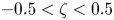 $-0.5<\zeta <0.5$,
  $(b)$
$(b)$  $S_2(\zeta -0.5)=E_2(\zeta )/E_2(0.5)= 4\zeta (1-\zeta )$ for
  $0<\zeta <1$,
  $(c)$
$(c)$  $S_3(\zeta -0.5)= -E_3(\zeta +0.5)/E_3(0)=\zeta (3-4\zeta ^2)$ for
  $-0.5<\zeta <0.5$, and
  $(d)$
$(d)$ 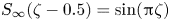 $S_\infty (\zeta -0.5)=\sin ({\rm \pi} \zeta )$, where
  $E_q$ is the Euler polynomial of degree
  $q$.
$q$.
The choice  $f_1(\zeta ) =S_\infty (\zeta -0.5)=\sin ({\rm \pi} \zeta )$ leads to the
  $C^\infty$ intrinsic mode
 \begin{equation} \left. \begin{gathered}
\begin{bmatrix} u_h \\ w_h \end{bmatrix} \propto
\sigma_{1} \begin{bmatrix} \cos{\rm \pi} x \: \sin{\rm \pi} z \\
-\sin{\rm \pi} x \: \cos{\rm \pi} z \end{bmatrix} \cos\sigma_1t, \\
\begin{bmatrix} p_h \\ \theta_h \end{bmatrix} \propto
\begin{bmatrix} (\lambda_{1}/{\rm \pi}) \sin{\rm \pi} x \: \sin{\rm \pi} z
\\ \sin{\rm \pi} x \: \cos{\rm \pi} z \end{bmatrix} \sin\sigma_1t,
\end{gathered} \right\} \end{equation}
\begin{equation} \left. \begin{gathered}
\begin{bmatrix} u_h \\ w_h \end{bmatrix} \propto
\sigma_{1} \begin{bmatrix} \cos{\rm \pi} x \: \sin{\rm \pi} z \\
-\sin{\rm \pi} x \: \cos{\rm \pi} z \end{bmatrix} \cos\sigma_1t, \\
\begin{bmatrix} p_h \\ \theta_h \end{bmatrix} \propto
\begin{bmatrix} (\lambda_{1}/{\rm \pi}) \sin{\rm \pi} x \: \sin{\rm \pi} z
\\ \sin{\rm \pi} x \: \cos{\rm \pi} z \end{bmatrix} \sin\sigma_1t,
\end{gathered} \right\} \end{equation}
with  $\sigma _1=1/\sqrt {2}$ and
  $\lambda _1=1/2$, which was shown to be excited by purely vertical forcing oscillations of the container (Yalim et al. Reference Yalim, Lopez and Welfert2018). In contrast, for the horizontal forcing considered here, the limit of the forced responses associated with the sequence
  $r=1-1/m$ with
  $m\ge 2$ corresponds to the quadratic spline
  $S_2$. Specifically,
 \begin{equation}
\lim_{m\to\infty} \dfrac{f_{1-1/m}(\zeta)}{f_{1-1/m}(0.5)}
= 4\zeta(1-|\zeta|)=S_2(\zeta-0.5), \quad |\zeta|\le1;
\end{equation}
\begin{equation}
\lim_{m\to\infty} \dfrac{f_{1-1/m}(\zeta)}{f_{1-1/m}(0.5)}
= 4\zeta(1-|\zeta|)=S_2(\zeta-0.5), \quad |\zeta|\le1;
\end{equation}
see Appendix C for a proof. The eigenmode components  $\eta _1$ and
  $\theta _1$ are visually indistinguishable from the bottom row of figure 9, obtained for
  $r=1-1/m$ with
  $m$ large.
The resonance at  $\omega ^2=1/2$ (i.e.
  $r=1$) corresponds to the largest peak in the Bode response diagram in figure 2
 $(a)$. Similar resonances occur for all rational values
  $r=n/m$ with both
  $m$ and
  $n$ odd integers, leading to other peaks in the Bode diagram at the corresponding values of
  $\omega ^2=\sigma _r^2=1/(1+r^2)$. These are all the cases for which Fredholm alternative A2 holds. The scaling relation
 \begin{equation} f_{n/m}(\zeta)=f_1(m\zeta), \end{equation}
shown in Appendix D, implies that the resulting mode, denoted  $M_{m:n}$, can be simply constructed from
  $M_{1:1}$, with vorticity and temperature deviation components
  $\eta _r$ and
  $\theta _r$ arranged in a regular
  $m\times n$ tiling of the scaled components of
  $M_{1:1}$.
Figure 11 shows the vorticity  $\eta _r$ and temperature deviation
  $\theta _r$ for the eigenmode
  $M_{5:3}$ resonating at squared frequency
 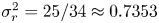 $\sigma _r^2=25/34\approx 0.7353$ (corresponding to
  $r=3/5$). The response consists of an exact
  $5\times 3$ tiling of copies of the components of the mode
  $M_{1:1}$, with piecewise linear
  $\eta _1$ in a pyramid pattern and piecewise quadratic
  $\theta _1$. The responses at slightly detuned frequencies on either side (slightly smaller and larger values of
  $r$) of the resonant modal case are also shown. These forced responses, being associated with rational values of
  $r$ that are approximations of the resonant case
  $r=3/5$, have piecewise constant
  $\eta _r$ and piecewise linear
  $\theta _r$. At the macroscopic scale of the figure, they appear to be smooth with one order of regularity higher than they actually possess. This is due to the natural visual (Riemann) integration of the small scales associated with the underlying network of characteristic lines emanating from the corners, resulting from the large values of
  $m$ and
  $n$ in the irreducible representation of
  $r=n/m$. Whereas the eigenmode has velocity and temperature fields of regularity class
  $C^1$ and satisfies the homogeneous linear inviscid system (4.1) in a pointwise or strong sense, the forced response at a detuned frequency has velocity and temperature fields only of class
  $C^0$ globally, as a result of the nature of the forcing, and are weak solutions.

Figure 11. Scaled waveform function  $f_r$ in
  $[-1.5,1.5]\times [-1.25,1.25]$ and associated scaled forced response (
 $\eta _r$ at phase 0 and
  $\theta _r$ at phase
  ${\rm \pi} /2$) for two values
 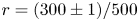 $r=(300\pm 1)/500$ close to
  $3/5$ (a,e,i,d,h,l) and eigenmode at
  $r=3/5$ (b,f,j,c,g,k, associated with opposite scaling). The blue curve is the 2-periodic extension of the red curve
  $f_r$ defined in the interval
  $[-(1+r)/2,(1+r)/2]$.
Note that the waveform functions  $f_r$ shown in figure 11 are normalized, with extrema at
  ${\pm }1$. In fact, the extrema of
  $f_r$ are, as in the case at
  $r=1$, unbounded at the resonant frequency. As the forcing frequency is varied across the resonant frequency, there is an inversion
  $f_r\to -f_r$. At resonance, the intrinsic mode of the unforced system is given by
 \begin{equation} \left. \begin{gathered} \begin{bmatrix} u_r \\ w_r \end{bmatrix} =\sigma_r\begin{bmatrix}r[\,f_r(x+rz)-f_r(x-rz)]\\ -f_r(x+rz)-f_r(x-rz)\end{bmatrix} \cos\sigma_rt, \\ \begin{bmatrix} p_r \\ \theta_r \end{bmatrix} =\begin{bmatrix} \lambda_r[F_r(x+rz)-F_r(x-rz)]\\ f_r(x+rz)+f_r(x-rz) \end{bmatrix} \sin\sigma_rt, \end{gathered} \right\} \end{equation}
obtained by letting  $\alpha =0$ in (4.7). So, the change in sign in
  $f_r$ is equivalent to a half-period phase shift in time. This is evident from comparing figures 11(a–d) and 11(i–l). Interestingly, this shift occurs in the high spatial frequency component of
  $f_r$, not the low spatial frequency component. This shift is emphasized in figures 11(b,f,j) and 11(c,g,k), representing the eigenmode, scaled to
  $\pm 1$ according to which side of the resonant frequency and the associated parameter
  $r=3/5$ they correspond. Also note how the cellular grid modal pattern of the piecewise quadratic temperature deviation
  $\theta _r$ becomes distorted along the characteristic directions and the cells merge upon detuning away from the resonance.
4.3. Spectral representations of modal and forced responses
The visual similarity between the quadratic spline  $S_2$ and the sine wave
  $S_\infty$ in figure 10 can be quantified via the sine Fourier series expansion (Olver et al. Reference Olver, Lozier, Boisvert and Clark2010, (24.8.4))
 \begin{align} S_2(\zeta-0.5)=\frac{32}{{\rm \pi}^3}\,\sum_{k\ge0} \frac{\sin(2k+1){\rm \pi}\zeta}{(2k+1)^3}\, =\frac{32}{{\rm \pi}^3}\,\left[S_\infty(\zeta-0.5)+ \frac{1}{3^3}S_\infty(3\zeta-0.5)+\ldots\right]. \end{align}
By approximating the factor  $32/{\rm \pi} ^3\approx 1.032\approx 1$ in (4.23), the resonating mode
  $M_{m:n}$ can be expanded as a superposition of an infinite number of
  $C^\infty$ intrinsic modes
  $I_{(2k+1)m:(2k+1)n}$. These are the odd spatial harmonics of
  $I_{m:n}$, all of which have the same intrinsic frequency
  $\sigma _{(2k+1)n/(2k+1)m}=\sigma _{n/m}$,
 \begin{equation} M_{m:n} \propto \sum_{\ell\ge0} (2\ell+1)^{{-}3}\, I_{(2\ell+1)m:(2\ell+1)n}. \end{equation}
The components  $(u_h, w_h, p_h, \theta _h)$ of the modes
  $I_{(2\ell +1)m:(2\ell +1)n}$ have the form
 \begin{equation}
\left. \begin{gathered} \begin{bmatrix}u_h\\
w_h\end{bmatrix} \propto
\sigma_{n/m}\begin{bmatrix}\dfrac{n}{m} \cos(2\ell+1)m{\rm \pi}
x \: \sin(2\ell+1)n{\rm \pi} z\\ -\sin(2\ell+1)m{\rm \pi} x \:
\cos(2\ell+1)n{\rm \pi} z\end{bmatrix} \cos\sigma_{n/m}t, \\
\begin{bmatrix}p_h\\ \theta_h\end{bmatrix} \propto
\begin{bmatrix} \dfrac{\lambda_{n/m}}{(2\ell+1)m{\rm \pi}}
\sin(2\ell+1)m{\rm \pi} x \: \sin(2\ell+1)n{\rm \pi} z\\
\sin(2\ell+1)m{\rm \pi} x \: \cos(2\ell+1)n{\rm \pi} z\end{bmatrix}
\sin\sigma_{n/m}t. \end{gathered} \right\}
\end{equation}
\begin{equation}
\left. \begin{gathered} \begin{bmatrix}u_h\\
w_h\end{bmatrix} \propto
\sigma_{n/m}\begin{bmatrix}\dfrac{n}{m} \cos(2\ell+1)m{\rm \pi}
x \: \sin(2\ell+1)n{\rm \pi} z\\ -\sin(2\ell+1)m{\rm \pi} x \:
\cos(2\ell+1)n{\rm \pi} z\end{bmatrix} \cos\sigma_{n/m}t, \\
\begin{bmatrix}p_h\\ \theta_h\end{bmatrix} \propto
\begin{bmatrix} \dfrac{\lambda_{n/m}}{(2\ell+1)m{\rm \pi}}
\sin(2\ell+1)m{\rm \pi} x \: \sin(2\ell+1)n{\rm \pi} z\\
\sin(2\ell+1)m{\rm \pi} x \: \cos(2\ell+1)n{\rm \pi} z\end{bmatrix}
\sin\sigma_{n/m}t. \end{gathered} \right\}
\end{equation} Figure 12 shows the vorticity and temperature deviation associated with the first few partial sums in the series expansion of  $M_{5:3}$ in (4.24), as well as of
  $M_{5:3}$, illustrating the rapid convergence of the series (4.23) and, thus, of (4.24). It is difficult to visually distinguish the primary fields, such as the temperature deviation, of
  $M_{m:n}$ from those of
  $I_{m:n}$. The contribution of terms beyond the first term in the expansion (4.24) is more visible for the vorticity due to the larger factor,
  $(2k+1)^{-2}$ vs.
  $(2k+1)^{-3}$, resulting from the term-wise differentiation of the velocity field.

Figure 12. Plots of the vorticity  $\eta _r$ and temperature deviation
  $\theta _r$ associated with the partial sums in the series expansion of
  $M_{5:3}$ in (4.24), for the number of indicated terms.
The expansion of forced responses in terms of odd harmonics of the sine wave can be obtained from the sine Fourier expansion
 \begin{equation} S_1(\zeta-0.5) ={-}\frac{1}{4}S'_2(\zeta) = \frac{8}{{\rm \pi}^2}\sum_{k\ge0}\frac{({-}1)^k}{(2k+1)^{2}}\sin(2k+1){\rm \pi}\zeta. \end{equation}
Expressing the linear spline as a superposition of  $m$ shifted triangular waves
  $S_1(\cdot -\zeta _j)$,
 \begin{equation} f_{n/m}(\zeta)=\sum_{j=1}^m a_j S_1(\zeta-\zeta_j), \end{equation}
where  $\zeta _j=(2j-1)/(2m)$,
  $j=1,\ldots ,m$ and
  $a_j={\pm }0.5$ are coefficients whose signs depend on
  $j$,
$j$,  $m$ and
  $n$ in a non-trivial way (see Appendix E), and substituting (4.26) into (4.27) leads to
 \begin{equation} f_{n/m}(\zeta) = \frac{4}{{\rm \pi}^2} \sum_{k\ge0}\frac{s_k}{(2k+1)^2}\sin(2k+1){\rm \pi}\zeta, \end{equation}
with
 \begin{equation} s_k = 2\sum_{j=1}^m a_j\sin(2k+1){\rm \pi}\zeta_j, \quad k\ge0. \end{equation}
The expression (4.29) amounts to a standard discrete sine transform of the coefficients  $a_j$ (the discrete sine transform denoted DST-IV in Britanak, Yip & Rao (Reference Britanak, Yip and Rao2007)). The closed form expression
 \begin{equation} s_k = ({-}1)^k \sec\left(\frac{2k+1}{2}\right)r{\rm \pi}, \end{equation}
with  $r=n/m$, is obtained and illustrated for the case
  $m=11$,
  $n=4$,
  $k=0$ in Appendix F. Note that
  $s_k$ remains finite as long as
  $(2k+1)r$ is not an odd integer, i.e.
  $r$ is not rational with
  $m$ and
  $n$ both odd. Using a density argument, the expression (4.30) extends to irrational values of
  $r$ (in which case the sequence
  $\{s_k\}_{k\ge 0}$ never repeats), so that
 \begin{equation} f_r(\zeta) = \frac{4}{{\rm \pi}^2}\sum_{k\ge0} \frac{({-}1)^k}{(2k+1)^2} \sec\left(\frac{2k+1}{2}\right)r{\rm \pi} \sin(2k+1)\zeta{\rm \pi}. \end{equation}
The waveform function is verified to be odd,  $f_r(-\zeta )=-f_r(\zeta )$. The relation
  $(-1)^k\sin (2k+1)\zeta {\rm \pi}=\cos (2k+1)(\zeta -0.5){\rm \pi}$ emphasizes the parity of
  $f_r$ around
  $\zeta =0.5$. Moreover, the direct verification that
  $f_r$ indeed satisfies (4.12) in the Fredholm alternative A1 reduces to a trivial trigonometric exercise, once the right-hand side of (4.12),
  $2x=S_1(x-0.5)$, is expanded for
  $|x|\le 0.5$ using (4.26). While the spectral approach employed in Maas & Lam (Reference Maas and Lam1995) and Wotherspoon (Reference Wotherspoon1995), valid for any
  $r$ different from resonant values
  $r=n/m$ with
  $m$ and
  $n$ odd integers, can be used to derive the infinite series expansion (4.31) directly from the functional relation (4.12), evaluating the series requires truncation to a finite number of terms and it is not clear how the truncation depends on
  $r$. On the other hand, the spatial approach leads to a linear system that provides an exact solution
  $f_r$, but only for rational
  $r=n/m$ with
  $m$ and
  $n$ of opposite parities. For irrational
  $r$, this system becomes unbounded and again a truncation, now to a finite system, must be made.
The value of (4.31) at  $\zeta =0.5$ is related to a secant zeta function introduced in Lalín, Rodrigue & Rogers (Reference Lalín, Rodrigue and Rogers2014) that motivated the recent study in Welfert (Reference Welfert2020), where it was shown that
  $f_{1/\sqrt {2}}(0.5)=1$, as observed in figure 8.
Replacing the quantity  $2x$ appearing in the components
  $w_r$,
  $p_r$ and
  $\theta _r$ of the forced response (4.15), hereby denoted
  $R_f$, by its expression in terms of the function
  $f_r$ from (4.12), and then substituting (4.31), shows that
  $R_f$ can be decomposed as the superposition of responses
  $R_{f_k}$,
 \begin{equation} R_f = \frac{4}{\rm \pi}\sum_{k\ge0} \frac{({-}1)^k}{2k+1}\, R_{f_k}, \end{equation}
of the sequence of linear forced systems
 \begin{equation} \left. \begin{gathered} \partial_t u_k ={-}\partial_x p_k + z\alpha\cos(2k+1){\rm \pi} x \sin\omega t,\\ \partial_t w_k ={-}\partial_z p_k + \theta_k,\\ \partial_t \theta_k ={-}w_k, \\ \partial_x u_k + \partial_z w_k = 0. \end{gathered} \right\} \end{equation}
An explicit expression of the components  $(u_k,w_k,p_k,\theta _k)$ of
  $R_{f_k}$ is given in Appendix G. The pointwise convergence of (4.32) away from characteristics inside the cavity also follows directly from the Fourier cosine expansion
 \begin{equation} S_0(x)=\frac{4}{\rm \pi}\sum_{k\ge0} \frac{({-}1)^k}{2k+1}\,\cos(2k+1){\rm \pi} x, \end{equation}
of the 2-periodic square wave  $S_0$, whose value is
  $(-1)^\ell$ for
  $x\in (\ell -0.5,\ell +0.5)$,
  $\ell \in \mathbb {Z}$, and, in particular,
  $1$ for
  $x\in (-0.5,0.5)$. The magnitude of the velocity components and temperature deviation of
  $R_{f_k}$ itself decreases inversely proportionally to
  $k$ (quadratically for the pressure); see (G5). In other words, the response to (4.33) vanishes for spatially highly oscillatory forcings. As a result, (4.32) converges absolutely, whereas (4.34) does not.
Figures 13 and 14 show the partial sums of (4.32) for the vorticity  $\eta$ and temperature deviation
  $\theta$, respectively, with an increasing number of terms, for the same
  $\sigma _r^2=\omega ^2$ values as those from figures 3 and 4. Note that in order to avoid
  $\sec (2k+1){\rm \pi} r=\infty$, the partial sums at
  $\sigma _r^2=0.1^+, 0.5^+, 0.9^-$ were computed using
  $\sigma _r^2$ values slightly detuned by a relative amount equivalent to ten times the machine epsilon (
 $10\times 2^{-52}$). Adding terms to the partial sums improves the approximation. The convergence depends on whether
  $\sec (2k+1){\rm \pi} r/2$ is large or not. For example, there is a big change for
  $\sigma _r^2=0.4$ when adding the fifth term and for
  $\sigma _r^2=0.6$ when adding the sixth term. This is particularly noticeable when
  $\sigma _r$ is very close to resonances. These near resonances occur when
  $(2k+1)r\approx 2\ell +1$, i.e. for every
  $k=m$ terms if
  $r\approx n/m$ with
  $m$ and
  $n$ both odd. For
  $\sigma _r^2=0.9^-$, (
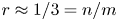 $r\approx 1/3=n/m$), the changes occur at terms
  $2$ (
$2$ ( $k=1$,
  $\ell =0$),
  $5$ (
$5$ ( $k=4$,
  $\ell =1$), etc.

Figure 13. Plots of the vorticity  $\eta _r$ associated with the partial sums in the series expansion of
  $R_f$ in (4.32), at
  $\sigma _r^2$ and a number of terms as indicated.

Figure 14. Plots of the temperature deviation  $\theta _r$ associated with the partial sums in the series expansion of
  $R_f$ in (4.32), at
  $\sigma _r^2$ and a number of terms as indicated.
For the most part, the comparison between the linear inviscid theory using 100 terms in the partial sums shown in figures 13 and 14 shows excellent agreement with the numerical results at the largest  $R_N=10^7$ shown in figures 3 and 4.
5. Comparison between viscous flow at large $R_N$ and inviscid flow

This section provides quantitative comparisons between the viscous nonlinear flows obtained via direct numerical simulations (DNS) and the linear inviscid theory. Global comparisons using the enstrophy and local comparisons using snapshots and horizontal profiles of the flows are made.
5.1. Inviscid versus viscous global enstrophy and a reduced-order viscous model
The global mean enstrophy  $\langle \mathcal {E}\rangle _\tau$, defined by (3.1), of the linear inviscid responses is now compared with that of the viscous responses obtained at increasing values of
  $R_N$ from figure 2
 $(a)$. The inviscid enstrophy is given by (for details, see Appendix H)
 \begin{equation} \langle\mathcal{E}\rangle_\tau = \frac{\alpha^2}{r^2\sigma_r^2} \sum_{k\ge0} \lambda_k^{{-}2} \left\{1+\frac{1+r^2}{2}\left[(1+r^2)\sec^2\lambda_k -(3-r^2) \frac{\tan\lambda_k}{\lambda_k}\right]\right\}. \end{equation}
The Dirichlet series (5.1) diverges at resonances which, for the square cavity, occur for every rational  $r=n/m$ with
  $m$ and
  $n$ both odd integers. Near a specific resonance,
  $\cos \lambda _k\approx 0$ for some
  $k$, (5.1) shows that the scaled global inviscid enstrophy,
  $(r/\alpha ^2)\langle \mathcal {E}\rangle _\tau ={O}(r^{-3}\sigma _r^{-2}[1+r^2]^2) ={O}([r+1/r]^3)$, is invariant under the transformation
  $r\leftrightarrow 1/r$, i.e.
  $\sigma _r^2\leftrightarrow 1-\sigma _r^2$. Figure 15
 $(a)$ illustrates this balance in the response magnitude between the
  $\sigma _r^2<0.5$ and
  $\sigma _r^2>0.5$ regimes. The graph is obtained by truncating the series (5.1) after 10 terms (
 $k=9$). This truncation only retains a finite subset of rational values
  $r=n/m$ at which the inviscid response becomes unbounded. However, truncating the infinite series after a fixed number of terms independent of
  $r$ allows for a larger set of resonances to be identified in the lower forcing frequency regime,
  $\sigma _r^2<0.5$, i.e.
  $r>1$, compared with the higher frequency regime,
  $\sigma _r^2>0.5$, because of the higher frequency in the variations of
  $\cos \lambda _k$. In contrast, truncating after
  $1+{O}(1/\sqrt {r})$ terms results in a comparable representation of the spatial variations of
  $\eta$ in the
  $x$ direction at
  $\sigma _r^2\approx 1$ and in the
  $z$ direction at
  $\sigma _r^2\approx 0$, making the graph and the various resonances visually symmetric approximately
  $\sigma _r^2=0.5$; see figure 15
 $(b)$. This modification in the number of terms increases the number of resonances detected by the truncated series in the
  $\sigma _r^2>0.5$ regime. For example, it decreases the frequency gap between consecutive resonances at
  $\sigma _r^2\approx 0.8$, with an inverse effect in the
  $\sigma _r^2<0.5$ regime, as can be observed from the increased gap around
  $\sigma _r^2\approx 0.2$. Increasing the proportionality constant of the
  ${O}(1/\sqrt {r})$ term allows for the representation of more oscillatory components throughout the
  $\sigma _r^2$ parameter inertial range, leading to many more resonances at
  $r=n/m$ with larger
  $n$ and
  $m$, including those closer to
  $\sigma _r^2=0.5$ (
 $r=1$), and defining an inviscid response ‘envelope’, shown in figure 15
 $(c)$. This figure also includes the synchronous (
 $\sigma _r^2=\omega ^2$) response curves from DNS at various
  $R_N$ from figure 2
 $(a)$, adjusted for viscous effects,
  $\delta (r/\alpha ^2)\langle \mathcal {E}\rangle _\tau$, where
 \begin{equation} \left. \begin{gathered} \delta = 0.8{\rm \pi}^2R_N^{{-}1/2} (0.25\lambda^{1.5}+0.75\lambda^6)^{{-}1}, \\ \lambda = 4\omega^2(1-\omega^2) =4\sigma_r^2(1-\sigma_r^2)=\left(\frac{2r}{1+r^2}\right)^2. \end{gathered} \right\} \end{equation}
The  ${O}(R_N^{-1/2})$ correction leads to the asymptotic collapse (away from lower-order resonant conditions) of the response curves from figure 2
 $(a)$ onto a single curve as
  $R_N$ increases, with the proportionality constant calibrated by the response at
  $\omega ^2=0.5$ (
 $\lambda =1$). The factor in
  $\delta$ inside the parentheses is a correction away from the
  $r=1$ case, in the spirit of the modal viscous reduced-order model used by Yalim et al. (Reference Yalim, Welfert and Lopez2019a), to obtain an approximate critical instability curve for the linearly stratified base state subjected to purely vertical oscillatory forcing of the container. The
  $\lambda ^{1.5}$ term controls the shape of the curves at
  $\omega ^2\approx 0$ or
  $1$, while the
  $\lambda ^6$ term controls their relative ‘flatness’ in the intermediate ranges around the values
  $0.25$ and
  $0.75$. Since
  $\lambda \le 1$, this mode-dependent correction factor is larger at
  $\omega ^2\approx 0$ and
  $1$, where the differences between the horizontal and vertical spatial scales of the responses are large, associated to the nearly vertical/horizontal characteristic directions, and for which the viscous boundary layers have a larger impact.

Figure 15. Graph of the enstrophy  $\langle \mathcal {E}\rangle _\tau$ from (5.1) scaled by
  $\alpha ^2/r$, evaluated at
  $10^6$ values
  $\omega ^2\in (0,1)$ using
  $(a)$
$(a)$  $1+9=10$ terms,
  $(b)$
$(b)$  $\lfloor 1+9/\sqrt {r}\rfloor$ term(s) or
  $(c)$
$(c)$  $\lfloor 1+99/\sqrt {r}\rfloor$ term(s) in the series, where
  $\lfloor x\rfloor$ represents the integer part of
  $x$. Also shown in
  $(c)$ are the scaled curves obtained from DNS for the different values of
  $R_N$ from figure 2 using the same colours, and a viscous correction factor
  $\gamma$ from (5.2). The supplementary movie 4 shows a frequency sweep of 9999 inviscid solutions uniformly distributed between
  $\omega ^2\in (0,1)$ at phase 0 for
  $\eta _r$ and phase
  ${\rm \pi} /2$ for
  $\theta _r$.
The 9999 frames in the supplementary movie 4 correspond to snapshots of  $\eta _r$ and
  $\theta _r$ at phases
  $0$ and
  ${\rm \pi} /2$, respectively, of the linear inviscid response flows at square forcing frequencies
  $\omega ^2\in (0,1)$. The animation provides a visual catalog of the Fredholm alternative A1 responses obtained from the truncated series (5.1) with
  $\lfloor 1+9/\sqrt {r}\rfloor$ term(s), where
  $\lfloor x\rfloor$ represents the integer part of
  $x$.
$x$.
5.2. Flow field comparisons
The nonlinear viscous DNS responses from figures 3 and 4 at  $R_N=10^7$ are now compared with the inviscid responses predicted by the analysis from § 4 at similar forcing frequencies
  $\omega$. These comparisons are shown in figures 16 and 17. All the inviscid responses shown were obtained using the discrete approach in physical space, described in Appendix B, rather than using the truncated spectral representations discussed in § 4.3. Responses associated with quadratic irrationals
  $r$ (e.g. for
 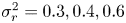 $\sigma _r^2=0.3,0.4,0.6$ and
  $0.7$) were obtained via approximations by a high-order convergent of appropriate continued fractions, similar to (4.16). Inviscid responses associated with rationals
  $r$ obtained from a lower-order convergent, which correspond to slightly detuned responses, are also included for comparison with viscous results obtained at smaller
  $R_N$. For example, the case
  $r=22/27$ in the vicinity of
  $\sigma _r^2=0.6$ is obtained from
  $r=4/5$ using the iteration
 \begin{equation} \begin{bmatrix} n\\m \end{bmatrix} \leftarrow \boldsymbol{\mathsf{R}}\begin{bmatrix} n\\m \end{bmatrix}, \quad \boldsymbol{\mathsf{R}}=\begin{bmatrix} 3 & 2 \\ 3 & 3 \end{bmatrix}, \end{equation}
while the case  $r=27/22$ in the vicinity of
  $\sigma _r^2=0.4$ is obtained from
  $r=5/4$ using a similar iteration based on
  $\boldsymbol{\mathsf{R}}^T$ instead. Note that the ratio of coefficients of the right eigenvector of
  $\boldsymbol{\mathsf{R}}$ is
  $r=\sqrt {2/3}$, while the same ratio for the left eigenvector is
  $r=\sqrt {3/2}$, values that are associated with the exact forcing frequencies.

Figure 16. Vorticity  $\eta$ from DNS at
  $R_N=10^7$
  $(a{,}c{,}e{,}g{,}i{,}k{,}m{,}o{,}q)$ and
  $\eta _r$ from the inviscid theory
  $(b{,}d{,}f{,}h{,}j{,}l{,}n{,}p{,}r)$, all at phase
  $0$, at the indicated squared forcing frequencies
  $\omega ^2$ (with the corresponding
  $r$ values indicated). The inviscid responses at
  $\sigma _r^2=0.3$,
  $0.4$,
  $0.6$ and
  $0.7$ are fractal and are obtained as limits of sequences with rational
  $r$.
$r$.

Figure 17. Temperature deviation  $\theta$ from DNS at
  $R_N=10^7$
 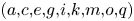 $(a{,}c{,}e{,}g{,}i{,}k{,}m{,}o{,}q)$ and
  $\theta _r$ from the inviscid theory
  $(b{,}d{,}f{,}h{,}j{,}l{,}n{,}p{,}r)$, all at phase
  ${\rm \pi} /2$, at the indicated squared forcing frequencies
  $\omega ^2$ (with the corresponding
  $r$ values indicated). The inviscid responses at
  $\sigma _r^2=0.3$,
  $0.4$,
  $0.6$ and
  $0.7$ are fractal and are obtained as limits of sequences with rational
  $r$.
$r$.
For ease of comparison, the viscous (DNS) results at large  $R_N=10^7$ from figures 3 and 4 have been reproduced in figures 16
 $(a{,}c{,}e{,}g{,}i{,}k{,}m{,}o{,}q)$ and 17
 $(a{,}c{,}e{,}g{,}i{,}k{,}m{,}o{,}q)$, albeit at the fixed phases of the forcing,
  $0$ for the vorticity
  $\eta$ and
  ${\rm \pi} /2$ for the temperature deviation
  $\theta$. For rational
  $r=n/m$ with sufficiently small
  $m$ and
  $n$, the DNS are very similar to the results predicted from the inviscid analysis shown in figures 16
 $(b{,}d{,}f{,}h{,}j{,}l{,}n{,}p{,}r)$ and 17
 $(b{,}d{,}f{,}h{,}j{,}l{,}n{,}p{,}r)$. For quadratic irrational
  $r$, such as
  $r=\sqrt {7/3}$,
  $\sqrt {3/2}$,
  $\sqrt {2/3}$ and
  $\sqrt {3/7}$, the DNS results at
  $R_N=10^7$ are unable to fully capture the fractal nature of the inviscid response. For finite
  $R_N$, the viscous effects smear out the small-scale details. The DNS responses appear more like the inviscid responses obtained at nearby rational values of
  $r=n/m$ with moderate
  $m$ and
  $n$, especially for
  $\eta$.
Over long periods of time, even small detunings in the forcing frequency can lead to sizeable phase differences in the responses and peaks in an inviscid response at one forcing frequency that may correspond to a minimal response at a nearby forcing frequency. In the viscous DNS responses, viscous detuning at small forcing amplitudes may lead to responses that are not perfect standing waves. Figure 18 illustrates such behaviour at  $\omega ^2=0.6$ and
  $R_N=10^7$. At phases
  $0$ and
  ${\rm \pi}$ (corresponding to fractions 0 and 0.50 of a forcing period for
  $\eta$) or
  ${\rm \pi} /2$ and
  $3{\rm \pi} /2$ (i.e. fractions
  $0.25$ and
  $0.75$ of a forcing period for
  $\theta$) the DNS response, already shown in figures 16 and 17, respectively, matches that expected from the inviscid prediction at that forcing frequency. However, at other phases, structures associated with inviscid responses at nearby
  $\sigma _r^2$ corresponding to
  $r=n/m$ with relatively small
  $m$ and
  $n$ appear to dominate. In particular, the structure associated with the resonant response at
  $r=9/11$ becomes clearly visible at phases where a standing wave response would be expected to vanish. Which inviscid response is identified in the DNS at a particular phase depends on the relative energies of the various responses at nearby (i.e. viscously detuned) forcing frequencies in relation to viscous effects as measured by
  $R_N$.

Figure 18. (g–v) Snapshots of  $\eta$ and
  $\theta$ from the DNS limit cycle at
  $R_N=10^7$ and
  $\omega ^2=0.6$ over one forcing period (see supplementary movies 1 and 2), while (a–f,w–z,aa,ab) show inviscid standing wave responses at maximal amplitude at
  $r$ and
  $\sigma _r^2$ values as indicated.
5.3. Horizontal profile comparisons
This subsection compares the horizontal profiles at  $z=0$ of the vorticity
  $\eta$ and temperature deviation
  $\theta$ from the DNS at
  $R_N=10^7$ with the linear inviscid theory. The comparison is performed at the maximal phase for the respective fields. In order to do this, the corresponding inviscid
  $\eta _r$ and
  $\theta _r$ need to be evaluated from the waveform function
  $f_r$. How these are evaluated depends on whether the response is forced or resonant.
For the forced responses, (4.15) results in
 \begin{equation}
\alpha^{{-}1}\begin{bmatrix} \eta_r \\ \theta_r
\end{bmatrix} = (1-\sigma_r^2)^{{-}1}
\begin{bmatrix}
\sigma_r^{{-}1}(\,f_r^\prime(x)-\sigma_r^2) \\
f_r(x)-x \end{bmatrix},
\end{equation}
\begin{equation}
\alpha^{{-}1}\begin{bmatrix} \eta_r \\ \theta_r
\end{bmatrix} = (1-\sigma_r^2)^{{-}1}
\begin{bmatrix}
\sigma_r^{{-}1}(\,f_r^\prime(x)-\sigma_r^2) \\
f_r(x)-x \end{bmatrix},
\end{equation}
with  $\eta _r$ affinely related to the derivative of
  $\theta _r$. For the resonant responses, (4.22) leads to
 \begin{equation} \begin{bmatrix} \eta_r \\ \theta_r \end{bmatrix} \propto 2 \begin{bmatrix} \sigma_r^{{-}1}f_r^\prime(x) \\ f_r(x) \end{bmatrix}, \end{equation}
with  $\eta _r$ now directly proportional to the derivative of
  $\theta _r$.
The profiles from the DNS and linear inviscid theory are shown in figure 19. The resonant responses are in figures 19(a,b) and 19(i,j) and the forced responses in figures 19(c,d) through 19(g,h). For  $\omega ^2=\sigma _r^2=0.5$ with
  $r=1/1$, the response is resonant and
  $f_r(x)=4x(1-|x|)$ for
  $|x|\le 0.5$ from (4.20). This waveform function
  $f_r$ is piecewise quadratic. Likewise, for
  $\omega ^2=\sigma _r^2=0.9$ with
  $r=1/3$, the response is resonant and (4.21) yields the piecewise quadratic
  $f_r(x)=4(3x)(1-3|x|)$ for
  $|x|\le 1/6$, and is extended by symmetry and periodicity for
  $|x|>1/6$. For the forced response at
  $\omega ^2=\sigma _r^2=0.8$ with rational
  $r=1/2$,
  $f_r(x)=|x+0.25|-|x-0.25|$ for
  $|x|\le 0.5$. This piecewise linear
  $f_r$ is obtained either by evaluating the spectral series (4.31) for
  $f_{1/2}$ in closed form, or by solving the system (4.14) and collecting the linear pieces.

Figure 19. Horizontal profiles of the (scaled) vorticity  $\eta$ and temperature deviation
  $\theta$ at
  $z=0$ and
  $\omega ^2$ as indicated. The black profiles correspond to the inviscid prediction based on the expression (4.22) (for a,b,i,j) or (4.15) (for c–h). The waveform function
  $f_r$ used in these expressions is obtained either explicitly for the cases
  $\omega ^2=0.5$,
  $0.8$ and
  $0.9$ associated with rational values of
  $r$, or via the series (4.31) truncated to the indicated number of terms for the cases
  $\omega ^2=0.6$ and
  $0.7$ associated with irrational values of
  $r$. An appropriate factor is used to scale the resonant cases (eigenmodes; a,b,i,j) in order to facilitate the comparison with the DNS response obtained at
  $R_N=10^7$ from figure 5 (here shown in cyan).
For the forced responses at  $\omega ^2=\sigma _r^2=0.6$ and
  $0.7$, for which
  $r$ is irrational, the evaluation of
  $f_r$ is no longer straightforward. The inviscid profiles that are illustrated in figures 19(c,d) and 19(e,f) were obtained by truncating the series representation of
  $f_r$, equation (4.31), as indicated in the figure. The number of terms retained is determined such that the resulting fields capture the oscillatory behaviour of the DNS responses without introducing high spatial frequency content due to large coefficients
  $\sec [(2k+1)/2]{\rm \pi} r$ for arbitrarily large
  $k$ when
  $r$ is irrational. While the truncation captures the oscillations in the DNS, it overestimates their amplitude. This is partly due to the inviscid theory not having viscous damping.
In order to improve the comparison, filtering techniques, such as the use of mollifiers (Tadmor Reference Tadmor2007), may be applied to the series representation of  $f_r$. The use of a mollifier softens the effects of the truncation and provides a much better quantitative account of the viscous results in the DNS. This is illustrated in figure 20, where the mollifier
  $\exp (-[(2k+1){\rm \pi} /40]^2)$ is used for
  $\omega ^2=\sigma _r^2=0.6$ and the mollifier
  $\exp (-[(2k+1){\rm \pi} /70]^4)$ is used for
  $\omega ^2=\sigma _r^2=0.7$. The factors 40 and 70 are fitting parameters, on the order of
  $R_N^{1/4}\approx 56$. These factors are consistent with the
  $R_N^{-1/2}$ factor appearing in the viscous dissipation correction (5.2) at the global enstrophy level. The power
  $2$ in the first mollifier corresponds to the Gaussian filtering associated with Laplacian dissipation. The power
  $4$ in the second mollifier corresponds to a biharmonic filtering, known for its scale selectivity. It is used extensively in ocean models (Griffies Reference Griffies2004), and its tendency to overshoot large changes in the data (Delhez & Deleersnijder Reference Delhez and Deleersnijder2007) is a feature exploited here to better capture the DNS results.

Figure 20. Horizontal profiles of the (scaled) vorticity  $\eta$ and temperature deviation
  $\theta$ at
  $z=0$ similar to figures 19(c,d) and 19(e,f), but using a mollifier rather than hard truncation of the spectral series (4.31) of the waveform function
  $f_r$ to account for viscous effects.
6. Summary, discussion and perspectives
6.1. Summary
A static vertically stratified fluid, with temperature  $T=z$, in a rectangular container is viscously stable. In order to have a sustained non-trivial response flow, the system needs to be continuously forced. The nature of the response flow depends on the nature of the forcing. Here, we consider the effects of subjecting the container to small horizontal oscillations that are harmonic in time, leading to a horizontally modulated effective gravity. The static stratified state is not an equilibrium of the forced system, and the response flow is non-trivial for all non-zero forcing frequencies
  $\omega$ and amplitudes
  $\alpha$. The flows obtained via DNS of the Navier–Stokes–Boussinesq equations are synchronous with the forcing and retain the spatio-temporal symmetries of the forced system. As viscous effects are reduced (by increasing
  $R_N$, the buoyancy frequency relative to the viscous time scale), these flows tend to be standing waves with spatial structure that is increasingly less regular, with nearly piecewise constant or piecewise linear vorticity distributions, depending on the forcing frequency.
The high  $R_N$ flows are well described in the inviscid limit by a perturbation analysis of the unforced equilibrium using the forcing amplitude as the small perturbation parameter. The forcing term in the full nonlinear problem,
  $\alpha T \sin \omega t$, reduces to
  $\alpha z \sin \omega t$ in the first-order perturbed system, which is linear and non-homogeneous with Dirichlet boundary conditions. This non-homogenous linear boundary value problem is reduced to a Poincaré equation for the temperature deviation, which is independent of the forcing.
The Poincaré equation is solved by a general standing wave ansatz for the temperature deviation, motivated by the DNS results. Substituting this into the first-order perturbation system leads to corresponding velocity components and pressure. Enforcing symmetries and boundary conditions on these then leads to a system of functional equations for the waveform function  $f$, one of which depends on the forcing. The solutions depend on whether the forcing resonates or not with the intrinsic modes of the static vertically stratified fluid in the container, as categorized by a Fredholm alternative for
  $f$. Forced responses are obtained at forcing frequency
  $\omega$ such that
  $\omega ^2=1/(1+r^2)$, with
  $r$ being irrational, or
  $r=n/m$ being rational with integers
  $m$ and
  $n$ of opposite parities. The linear inviscid system has then a unique response flow (alternative A1) which scales with the forcing amplitude
  $\alpha$. For rational
  $r=n/m$ with
  $m$ and
  $n$ of opposite parities, a linear spline
  $f$ can be determined by solving a non-homogeneous linear system. The resulting response has piecewise constant vorticity which is discontinuous across characteristic lines and forms a regular harlequin pattern. For irrational
  $r$, the waveform function
  $f$ is better expressed in the form of a spectral Dirichlet series. At least for quadratic irrationals
  $r$, the sequence of rational cumulants of the continued fraction representation of
  $r$ leads to self-similar properties of
  $f$ and the harlequin pattern of the vorticity becomes fractal.
Resonant responses are obtained at forcing frequencies  $\omega ^2=1/(1+r^2)$ for
  $r=n/m$ with integers
  $m$ and
  $n$ both odd (alternative A2). These responses correspond to solutions of the unforced, homogeneous inviscid linear perturbation equations and are intrinsic eigenmodes of the unforced system. The spatial structure of the specific modes excited by the particular forcing is obtained by considering the limit of forced responses as the forcing frequency approaches a resonant frequency. The response flow becomes unbounded, with piecewise quadratic velocity and temperature deviation, and, thus, a piecewise linear vorticity field, and can be represented as a superposition of an infinite set of odd spatial harmonics of smooth intrinsic modes of the unforced system.
Models of viscous dissipation both at the global enstrophy level and at the local level in a horizontal cut via mollifiers were introduced in the inviscid model to account for viscous effects at finite  $R_N$. The use of filtering strategies in post-processing is in general necessary when differentiating low regularity solutions.
6.2. Discussion
The linear inviscid theory provides an increasingly more accurate description of the DNS responses as  $R_N$ is increased, highlighting the tendency of these DNS response flows to become less regular, and even fractal-like for certain forcing frequencies, as viscous regularization is reduced. These non-smooth flow features originate in the existence of non-smooth solutions of the Poincaré equation, a possibility already raised by Aldridge (Reference Aldridge1975). Low regularity solutions were obtained in Maas & Lam (Reference Maas and Lam1995) by solving the Poincaré equation in a geometry with at least one wall oblique to the direction of stratification or the direction perpendicular to the stratification, with homogeneous (Dirichlet) boundary conditions specified at the boundaries. In the present study the square cavity considered has all walls either parallel or orthogonal to gravity and the low regularity of the solutions is a consequence of the oscillatory horizontal forcing being orthogonal to the direction of gravity.
Solutions with low regularity that have been observed in stratified as well as rotating flows are more typically beams with a concentrated delta-like distribution of vorticity along rays (in two dimensions) or vortex sheets (in three dimensions). These beams usually originate from localized forcings and are aligned with the characteristics, typically forming a St Andrew's cross pattern (Görtler Reference Görtler1943; Mowbray & Rarity Reference Mowbray and Rarity1967; Voisin Reference Voisin2003). The piecewise constant vorticity solutions obtained here constitute a more regular class of beams, with energy distributed over the container rather than focused in rays or sheets, and can be overshadowed by these stronger beams when the latter are present, as happens, for example, in numerical simulations of parametrically forced rotating flows (Wu et al. Reference Wu, Welfert and Lopez2020).
The present study has focused on the very small forcing amplitude regime. The question of what happens as this amplitude is increased remains open, and of current interest (e.g. Savaro et al. Reference Savaro, Campagne, Linares, Augier, Sommeria, Valran, Viboud and Mordant2020). The transition to internal wave turbulence is expected to occur at smaller forcing amplitudes as  $R_N$ is increased as a result of higher-order resonances becoming less viscously damped (Aldridge & Toomre Reference Aldridge and Toomre1969). We are currently investigating how the response flows lose stability as the forcing amplitude is increased.
When  $r=n/m$, with integers
  $m$ and
  $n$ of opposite parities, the linear inviscid system (4.1) admits, under alternative A1, a unique synchronous forced response that scales with the forcing amplitude. However, (4.1) also admits solutions which are not standing waves for such values of
  $r$, for example, a superharmonic component evolving at twice the forcing frequency,
  $2\omega$, if
  $4\omega ^2<1$. The spatio-temporal symmetries then allow for superharmonic resonant responses under alternative A2. Such a resonance is triggered by second-order nonlinear contributions, but it is moderated by viscous effects. For large values of
  $R_N$ (larger than those considered in the present study for the very low forcing amplitude
  $\alpha$ used), it is expected that viscous damping is sufficiently reduced so that the superharmonic resonant response will dominate.
6.3. Extensions and further remarks
In the present study we have considered the square cavity. However, the results are straightforwardly extended to rectangular cavities of width-to-depth aspect ratio  $\varGamma$. The dispersion relation (4.5) then becomes
  $\sigma _r^2=\varGamma ^2/(\varGamma ^2+r^2)$, with responses according to Fredholm alternatives A1 and A2 depending on
  $r$ in a similar fashion as when
  $\varGamma =1$. If the container is not rectangular, for example, due to walls at oblique angles to gravity, or is tilted, the responses may become non-trivial as a result of the peculiar reflections of internal waves, which may lead to internal wave attractors or focusing into edges or corners. While some aspects of this has been previously studied (e.g. Maas & Lam Reference Maas and Lam1995; Wotherspoon Reference Wotherspoon1995), there is still much to learn (e.g. Bajars et al. Reference Bajars, Frank and Maas2013; Pillet et al. Reference Pillet, Ermanyuk, Maas, Sibgatullin and Dauxois2018; Pillet, Maas & Dauxois Reference Pillet, Maas and Dauxois2019), and approaches from the study of how inertial waves reflect in the obliquely rotating cube (Wu et al. Reference Wu, Welfert and Lopez2020) can be adapted for the internal wave problem.
In order to determine whether the low regularity patterns in the 2-D solutions persist in a 3-D container, two cases, corresponding to  $\omega ^2=0.2$ and
  $\omega ^2=0.5$, were simulated at
  $R_N=10^6$ and
  $\alpha =1.75\times 10^{-6}$ in a box
  $[-0.5,0.5]\times [-0.2,0.2]\times [-0.5,0.5]$ with no-slip, insulated walls at
  $y=\pm 0.2$. The spanwise aspect ratio
  $0.4$ is the same as that used in the experiments of Benielli & Sommeria (Reference Benielli and Sommeria1998) and the simulations of Yalim et al. (Reference Yalim, Lopez and Welfert2020) for the vertically forced system. The
  $\omega ^2=0.2$ case is a prototypical example of a forced response in the 2-D setting (Fredholm alternative A1), and the
  $\omega ^2=0.5$ case corresponds to a resonant response associated with the main peak in the Bode diagram (figure 2) in the 2-D setting (Fredholm alternative A2). Figure 21(a–d) shows the 2-D DNS solutions from figures 3 and 4 for comparison with the figure 21(e–h) showing the vorticity and temperature deviation at the spanwise midplane
  $y=0$ of the 3-D DNS solutions. For
  $\omega ^2=0.2$, the solutions are qualitatively the same and quantitatively the 3-D vorticity level is approximately
  $77\,\%$ that of the 2-D vorticity, while the 3-D temperature deviation is approximately
  $2\,\%$ larger. For
  $\omega ^2=0.5$, the solutions are also qualitatively the same, but the 3-D vorticity and temperature deviation levels are both approximately
  $46\,\%$ those of the corresponding 2-D solution. From the 2-D study, it appears that resonant responses tend to be more affected by viscous effects than the forced responses are. The viscous dissipation in the boundary layers along the spanwise walls of the 3-D container are also responsible for dampening the response. This warrants a more detailed separate investigation. As noted by Benielli & Sommeria (Reference Benielli and Sommeria1998), the effects of friction in parametrically forced stratified confined flows are not well understood, and, hence, neither are those associated with variations of the Prandtl number.

Figure 21. Panels (a–d) show the 2-D  $\eta$ and
  $\theta$ at
  $R_N=10^6$ and
  $\omega^2$ as indicated (repeated from figures 3 and 4 for ease of comparison) and panels (e–g) show the 3-D
  $\eta$ and
  $\theta$ in the spanwise midplane using the same colour levels as in the 2-D cases (a–d). Panels (i–l) show the corresponding isosurfaces of the 3-D solutions (using a different colour map), with the boundary layer regions clipped.
Supplementary movies
Supplementary movies are available at https://doi.org/10.1017/jfm.2021.73.
Acknowledgements
We thank ASU Research Computing facilities and the NSF XSEDE programme for the computing resources. We also thank the editor and the referees for insightful comments and suggestions that led us to present this work in a broader context.
Declaration of interests
The authors report no conflict of interest.
Appendix A. The relation between $f_{1/r}$ and $f_r$ and the corresponding flow responses


If  $f_r$ is odd and obeys (4.10) and (4.12), then the function
  $f_{1/r}$ defined by
 \begin{equation} f_{1/r}(\zeta) = \zeta - \frac{1}{r}\,f_r(r\zeta), \quad |\zeta|\le \frac{1+r}{2r}, \end{equation}
is also odd and obeys (4.10) and (4.12). To see this, assume that  $f_r:[-(1+r)/2,(1+r)/2]\to \mathbb {R}$ is odd and obeys the conditions
 \begin{equation} f_r(\xi+0.5)+f_r(\xi-0.5)=2\gamma\xi, \quad |\xi|\le r/2, \end{equation}
 \begin{equation}f_r(x+r/2)+f_r(x-r/2)=2(1-\gamma)x, \quad |x|\le0.5, \end{equation}
where  $\gamma \in \mathbb {R}$. We show that the function
  $f_{1/r}$, defined by (A1), obeys similar properties in appropriate ranges of its argument. For
  $|\xi |\le 1/(2r)$, we obtain
 \begin{align}
f_{1/r}(\xi+0.5)+f_{1/r}(\xi-0.5)
&=2\xi-[\,f_r(x+r/2)+f_r(x-r/2)]/r \nonumber\\
&=2\xi-2(1-\gamma)x/r=2\gamma\xi,
\end{align}
\begin{align}
f_{1/r}(\xi+0.5)+f_{1/r}(\xi-0.5)
&=2\xi-[\,f_r(x+r/2)+f_r(x-r/2)]/r \nonumber\\
&=2\xi-2(1-\gamma)x/r=2\gamma\xi,
\end{align}
here  $x=r\xi$ with
  $|x|\le 0.5$. On the other hand,
 \begin{align}
f_{1/r}(x+0.5)+f_{1/r}(x-0.5)
&=2x-[\,f_r(\xi+0.5)+f_r(\xi-0.5)]/r \nonumber\\ &=2x-2\gamma
\xi/r=2(1-\gamma)x
\end{align}
\begin{align}
f_{1/r}(x+0.5)+f_{1/r}(x-0.5)
&=2x-[\,f_r(\xi+0.5)+f_r(\xi-0.5)]/r \nonumber\\ &=2x-2\gamma
\xi/r=2(1-\gamma)x
\end{align}
for  $\xi =rx$ with
  $|\xi |\le r/2$ and
  $|x|\le 0.5$. For
  $\gamma =0$, (A2) and (A3) are then equivalent to (4.10) and (4.12), respectively.
The relation (A1) is involutory,  $f_{1/(1/r)}=f_r$ on the interval
  $[-(1+r)/2,(1+r)/2]$, and this provides a direct connection between the corresponding velocities of the forced responses at
  $r$ (with frequency
  $\sigma _r$) and at
  $1/r$ (with frequency
  $\sigma _{1/r}=\sqrt {|1/2-\sigma _r^2|}$), namely
 \begin{equation} \begin{bmatrix} u_{1/r}(z,x,t) \\ w_{1/r}(z,x,t) \end{bmatrix} =\dfrac{r\cos(r\sigma_rt)}{\cos(\sigma_rt)} \begin{bmatrix} w_r(x,z,t) \\ u_r(x,z,t) \end{bmatrix}. \end{equation}
The relations between  $(p_{1/r}, \theta _{1/r})$ and
  $(p_r,\theta _r)$ are not as straightforward. In particular,
  $\theta _{1/r}$ cannot be simply related to
  $\theta _r$, and
  $p_{1/r}$ is only related to
  $p_r$ up to a quadratic pressure term proportional to
  $\alpha$. Nevertheless, the identity (A1) shows that the response (4.15) associated with
  $1/r>1$ can be reconstructed from that obtained for
  $r<1$. In particular, (A6) shows that the velocity oscillation amplitude associated with
  $1/r$ is
  $r$ times that of the velocity oscillation amplitude associated with
  $r$. For
  $0 < r < 1$, the vorticity response at forcing frequency
  $\omega ^2=\sigma _{1/r}^2<1/2$ oscillates at lower amplitude and angular frequency,
  $\eta _{1/r}(z,x,t)\sim -r\eta _r(x,z,t)$ and
  $r\sigma _r$, than the vorticity response
  $\eta _r(x,z,t)$ at
  $\omega ^2=\sigma _r^2>1/2$. This accounts for the tendency in the
  $\langle \mathcal {E}\rangle _\tau$ vs.
  $\omega ^2$ response curves shown in figure 2
 $(a)$ to slightly increase (on a logarithmic scale) in proportion to
  $1/r=\sqrt {(1-\omega ^2)/\omega ^2}$, rather than
  $1/r^2$. This is more markedly visible at small
  $\omega$.
The relation (A1) can be used to determine  $f_r(\zeta )=\zeta -rf_{1/r}(\zeta /r)$ from
  $f_{1/r}$ for
  $r>1$, i.e.
  $\omega ^2<0.5$. The knots
  $\zeta$ of
  $f_r$ are related to the knots
  $x=\zeta /r$ of
  $f_{1/r}$ by
  $\zeta =rx$, and the corresponding value of
  $f_r$ becomes
  $f_r(\zeta )=rx-rf_{1/r}(x)$. The relations
 \begin{equation} \sigma_{1/r}=r\sigma_r \quad\text{and}\quad c_{1/r}=r^2c_r \end{equation}
then show that
 \begin{align}
\dfrac{1}{\cos r\sigma_rt} \begin{bmatrix}u_{1/r}(z,x,t)\\
w_{1/r}(z,x,t)\end{bmatrix} &=c_{1/r}\sigma_{1/r}
\begin{bmatrix} [\,f_{1/r}(z+x/r)-f_{1/r}(z-x/r)]/r\\
2z-f_{1/r}(z+x/r)-f_{1/r}(z-x/r)\end{bmatrix}\nonumber\\
&=r^2c_r\sigma_r\begin{bmatrix}2-f_r(x+rz)+f_r(x-rz)\\
f_r(x+rz)-f_r(x-rz)\end{bmatrix}\nonumber\\
&=\frac{r}{\cos\sigma_rt} \begin{bmatrix}w_r(x,z,t)\\
u_r(x,z,t)\end{bmatrix}.
\end{align}
\begin{align}
\dfrac{1}{\cos r\sigma_rt} \begin{bmatrix}u_{1/r}(z,x,t)\\
w_{1/r}(z,x,t)\end{bmatrix} &=c_{1/r}\sigma_{1/r}
\begin{bmatrix} [\,f_{1/r}(z+x/r)-f_{1/r}(z-x/r)]/r\\
2z-f_{1/r}(z+x/r)-f_{1/r}(z-x/r)\end{bmatrix}\nonumber\\
&=r^2c_r\sigma_r\begin{bmatrix}2-f_r(x+rz)+f_r(x-rz)\\
f_r(x+rz)-f_r(x-rz)\end{bmatrix}\nonumber\\
&=\frac{r}{\cos\sigma_rt} \begin{bmatrix}w_r(x,z,t)\\
u_r(x,z,t)\end{bmatrix}.
\end{align}A direct consequence of (A8) is the relation between the corresponding vorticities,
 \begin{equation} \eta_{1/r}(z,x,t)={-}\frac{r\cos r\sigma_r t}{\cos\sigma_r t} \eta_r(x,y,t). \end{equation}
Appendix B. The linear system (4.14) and its solution
We illustrate the construction and solution of the linear system (4.14) obtained by enforcing the condition (4.12) arising from the Fredholm alternative A1 in the rational case  $r=n/m$ with
  $m=11$ and
  $n=4$.
Let 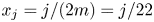 $x_j=j/(2m)=j/22$ and
  $f_j=f(x_j)$ for
  $j\in \mathbb {Z}$. Evaluating (4.12) at
  $x_j$,
  $j=1,\ldots ,11$, yields the system

The parity conditions  $f_{-j}=-f_j$,
  $j=0,1,2,3$ (in particular,
  $f_0=0$) and symmetries
  $f_{11+j}=f_{11-j}$,
  $j=1,2,3,4$, reduce (
) to the  $m\times m=11\times 11$ system (4.14),
 \begin{equation}
\renewcommand{\arraystretch}{.9}
\boldsymbol{\mathsf{A}}\boldsymbol{f}(\boldsymbol{x})
= \left[\begin{array}{@{}c@{}c@{}c@{\;}cccccccc@{}} & & -1
& & 1 & & & & & & \\ & -1 & & & & 1 & & & & & \\ -1 & & & &
& & 1 & & & & \\ & & & & & & & 1 & & & \\ 1 & & & & & & & &
1 & & \\ & 1 & & & & & & & & 1 & \\ & & 1 & & & & & & & &
1\\ & & & 1 & & & & & & 1 & \\ & & & & 1 & & & & 1 & & \\ &
& & & & 1 & & 1 & & & \\ & & & & & & 2 & & & &
\end{array}\right] \begin{bmatrix}
f_1\\f_2\\f_3\\f_4\\f_5\\f_6\\f_7\\f_8\\f_9\\f_{10}\\ \,f_{11}
\end{bmatrix} =2\begin{bmatrix}
x_1\\x_2\\x_3\\x_4\\x_5\\x_6\\x_7\\x_8\\x_9\\x_{10}\\x_{11}\end{bmatrix}
=2\boldsymbol{x},
\end{equation}
\begin{equation}
\renewcommand{\arraystretch}{.9}
\boldsymbol{\mathsf{A}}\boldsymbol{f}(\boldsymbol{x})
= \left[\begin{array}{@{}c@{}c@{}c@{\;}cccccccc@{}} & & -1
& & 1 & & & & & & \\ & -1 & & & & 1 & & & & & \\ -1 & & & &
& & 1 & & & & \\ & & & & & & & 1 & & & \\ 1 & & & & & & & &
1 & & \\ & 1 & & & & & & & & 1 & \\ & & 1 & & & & & & & &
1\\ & & & 1 & & & & & & 1 & \\ & & & & 1 & & & & 1 & & \\ &
& & & & 1 & & 1 & & & \\ & & & & & & 2 & & & &
\end{array}\right] \begin{bmatrix}
f_1\\f_2\\f_3\\f_4\\f_5\\f_6\\f_7\\f_8\\f_9\\f_{10}\\ \,f_{11}
\end{bmatrix} =2\begin{bmatrix}
x_1\\x_2\\x_3\\x_4\\x_5\\x_6\\x_7\\x_8\\x_9\\x_{10}\\x_{11}\end{bmatrix}
=2\boldsymbol{x},
\end{equation}obtained by mirroring columns of the matrix in (
B1) around the greyed-out columns. The system (B2) can be split into two independent subsystems for odd- and even-indexed values (a consequence of  $m$ and
  $n$ having opposite parities),
 \begin{equation} \renewcommand{\arraystretch}{.9} \left[\begin{array}{@{}c@{}ccccc@{}} & -1 & 1 & & & \\ -1 & & & 1 & & \\ 1 & & & & 1 & \\ & 1 & & & & 1\\ & & 1 & & 1 & \\ & & & 2 & & \end{array}\right] \begin{bmatrix}f_1\\f_3\\f_5\\f_7\\f_9\\\,f_{11}\end{bmatrix} =2\begin{bmatrix}x_1\\x_3\\x_5\\x_7\\x_9\\x_{11}\end{bmatrix}, \quad \left[\begin{array}{@{}c@{}cccc@{}} -1 & & 1 & & \\ & & & 1 & \\ 1 & & & & 1\\ & 1 & & & 1\\ & & 1 & 1 & \end{array}\right] \begin{bmatrix}f_2\\f_4\\f_6\\f_8\\\,f_{10}\end{bmatrix} =2\begin{bmatrix}x_2\\x_4\\x_6\\x_8\\x_{10}\end{bmatrix}. \end{equation}
The two subsystems can in turn be permuted into lower triangular bidiagonal systems,
 \begin{equation} \renewcommand{\arraystretch}{.9}
\left[\begin{array}{@{}c@{\;}c@{\;}cc@{\;}c@{\;}c@{}} 2 & &
& & & \\ 1 & -1 & & & & \\ & 1 & 1 & & & \\ & & 1 & 1 & &
\\ & & & 1 & -1 & \\ & & & & 1 & 1 \end{array}\right]
\begin{bmatrix}f_7\\f_1\\f_9\\f_5\\f_3\\\,f_{11}\end{bmatrix}
=2\begin{bmatrix}x_{11}\\x_3\\x_5\\x_9\\x_1\\x_7\end{bmatrix},
\quad \left[\begin{array}{@{}cc@{\;}c@{\;}cc@{}} 1 & & & &
\\ 1 & 1 & & & \\ & 1 & -1 & & \\ & & 1 & 1 & \\ & & & 1 &
1 \end{array}\right]
\begin{bmatrix}f_8\\f_6\\f_2\\\,f_{10}\\\,f_4\end{bmatrix}
=2\begin{bmatrix}x_4\\x_{10}\\x_2\\x_6\\x_8\end{bmatrix},
\end{equation}
\begin{equation} \renewcommand{\arraystretch}{.9}
\left[\begin{array}{@{}c@{\;}c@{\;}cc@{\;}c@{\;}c@{}} 2 & &
& & & \\ 1 & -1 & & & & \\ & 1 & 1 & & & \\ & & 1 & 1 & &
\\ & & & 1 & -1 & \\ & & & & 1 & 1 \end{array}\right]
\begin{bmatrix}f_7\\f_1\\f_9\\f_5\\f_3\\\,f_{11}\end{bmatrix}
=2\begin{bmatrix}x_{11}\\x_3\\x_5\\x_9\\x_1\\x_7\end{bmatrix},
\quad \left[\begin{array}{@{}cc@{\;}c@{\;}cc@{}} 1 & & & &
\\ 1 & 1 & & & \\ & 1 & -1 & & \\ & & 1 & 1 & \\ & & & 1 &
1 \end{array}\right]
\begin{bmatrix}f_8\\f_6\\f_2\\\,f_{10}\\\,f_4\end{bmatrix}
=2\begin{bmatrix}x_4\\x_{10}\\x_2\\x_6\\x_8\end{bmatrix},
\end{equation}with (re-ordered) solutions
 \begin{equation} \renewcommand{\arraystretch}{.9} \begin{bmatrix}f_1\\f_3\\f_5\\f_7\\f_9\\\,f_{11}\end{bmatrix} =\frac{1}{22}\begin{bmatrix}5\\11\\13\\11\\5\\3\end{bmatrix}, \quad \begin{bmatrix}f_2\\f_4\\f_6\\f_8\\\,f_{10}\end{bmatrix} =\dfrac{1}{22}\begin{bmatrix}8\\12\\12\\8\\4\end{bmatrix} =\dfrac{1}{2} \begin{bmatrix}1 & 1 & & & & \\ & 1 & 1 & & & \\ & & 1 & 1 & & \\ & & & 1 & 1 & \\ & & & & 1 & 1\end{bmatrix} \begin{bmatrix}f_1\\f_3\\f_5\\f_7\\f_9\\\,f_{11}\end{bmatrix}. \end{equation}
The connection between odd- and even-indexed values  $f_j$ exposed by (B5a,b) shows that the 2-periodic linear spline
  $f$ interpolating
  $(x_j,f_j)$ is fully determined, in the case
  $m=11$,
  $n=4$, by the odd-indexed values
  $f_j$,
  $j=1,3,\ldots ,11$, alone; see figure 22. This property generalizes to other pairs
  $(m,n)$ with
  $m$ and
  $n$ of opposite parities, with the linear spline completely determined by the set of values
  $f_j$ such that
  $j$ has the same parity as
  $m$.
$m$.

Figure 22. The 2-periodic linear spline  $f_{4/11}$. The dots indicate the interpolating points. All data can be obtained from
  $(x_j,f_j)$,
  $j=1,3,5,7,9$ and
  $11$, via the symmetries approximately
  $x=0$ and
  $x=0.5$. The range of
  $x$-values associated with the red part is the range
  $[-(1+4/11)/2,(1+4/11)/2]\approx [-0.68,0.68]$ where
  $f$ must be defined in order to evaluate the response everywhere in the square cavity.
The inconsistency of the system (4.14) when  $r=m/n$ with both
  $m$ and
  $n$ odd is argued in § 4.2 for the case
  $m=n=1$. For completeness, it is also illustrated here for
  $m=5$ and
  $n=3$. The system

for  $f_j=f(x_j)$ at
  $x_j=j/10$ is similar to (B1), and now folds into the system
 \begin{equation} \renewcommand{\arraystretch}{.9} \boldsymbol{\mathsf{A}}\boldsymbol{f}(\boldsymbol{x}) = \left[\begin{array}{@{}c@{}c@{}c@{\;}ccccc@{}} & -1 & & & 1\\ -1 & & & 1 & \\ & & 1 & & \\ 1 & 1 & & & \\ 1 & 1 & & & \end{array}\right] \begin{bmatrix} f_1\\f_2\\f_3\\f_4\\\,f_5 \end{bmatrix} =2\begin{bmatrix} x_1\\x_2\\x_3\\x_4\\x_5\end{bmatrix}, \end{equation}
using the parity conditions  $f_{-j}=-f_j$,
  $j=0,1,2$, and symmetries
  $f_{5+j}=f_{5-j}$,
  $j=1,2,3,4$. The system (B7) is inconsistent, in view of its last two equations. In this case alternative A1 fails and alternative A2 holds, leading to a resonant response.
Appendix C. Proof of (4.20)
For  $r=1-1/m$ with
  $m>1$ (i.e.
  $n=m-1$), the system (4.14) becomes

with  $x_j=j/(2m)$,
  $f_j=f(x_j)$,
  $j=1,\ldots ,m$ and
  $f=f_{1-1/m}$; see Appendix B for the construction of this system. This system is easily solved via backward substitution, i.e.
 \begin{equation} f_j = j/2-\lfloor \kern1.5pt j/2\rfloor\lceil j/2\rceil/m, \quad j=1,\ldots,m, \end{equation}
where  $\lfloor \cdot \rfloor$ and
  $\lceil \cdot \rceil$ denote the floor and ceiling functions (functions which take a real argument and return the greatest/least integer less/greater than or equal to the argument, respectively). In particular, the maximal value over all
  $j$ is obtained for
  $j=m$ at
  $x_m=0.5$,
 \begin{equation} f_m = m/2-\lfloor m/2\rfloor\lceil m/2\rceil/m= m/4 + \begin{cases} 0 & \text{if } m \ \text{even},\\ 1/(4m) & \text{if } m \ \text{odd}. \end{cases} \end{equation}
For  $j=j(m)$ such that
  $x_j\to x\in [0,0.5]$ as
  $m\to \infty$,
  $\lfloor \kern1.5pt j/2\rfloor /m \to x$,
  $\lceil j/2\rceil /m \to x$ and
 \begin{equation} f_j/(m/4)=4x_j-4(\lfloor \kern1.5pt j/2\rfloor/m)(\lceil j/2\rceil/m)\to 4x-4x^2=4x(1-x), \end{equation}
so that  $f_j/f_m\to 4x(1-x)$ as well. Using
  $f(-x)=-f(x)$ and
  $f(0.5+x)=f(0.5-x)$ for
  $|x|\le 0.5-1/(2m)$ shows that, in the limit
  $m\to \infty$,
  $f$ satisfies (4.20).
The right-hand side function of (4.20) is the quadratic Euler spline  $S_2(x-0.5)$ (Olver et al. Reference Olver, Lozier, Boisvert and Clark2010, equation 24.17.3). The first
  $m-1$ equations in the system (C1) can then be interpreted as a central-finite-difference discretization of the boundary value problem
 \begin{equation} \tilde{f}'(x)=S_2'(x)=4-8x, \quad 0 < x < 0.5, \quad \tilde{f}(0)=0, \end{equation}
for the scaled function  $\tilde {f}=(4/m)f$. The last equation corresponds to an odd parity condition at
  $0$.
$0$.
Appendix D. Proof that (4.21) is odd and satisfies (4.10) and (4.13) when $m$ and $n$ are odd and $f_1$ is $1$-antiperiodic


The odd parity of  $f_{n/m}$ defined by (4.21) follows from that of
  $f_1$. Next, note that the
  $1$-antiperiodicity of
  $f_1$ implies that it satisfies (4.13) for all
  $x$, not just
  $|x|\le 0.5$. Then, for
  $m=2m'+1$ an odd integer,
 \begin{align}
f_{n/m}(0.5+x)
&=f_1(m/2+mx)=({-}1)^{m'}f_1(0.5+mx)\nonumber\\
&=({-}1)^{m'}f_1(0.5-mx)=f_1(m/2-mx)=f_{n/m}(0.5-x),
\end{align}
\begin{align}
f_{n/m}(0.5+x)
&=f_1(m/2+mx)=({-}1)^{m'}f_1(0.5+mx)\nonumber\\
&=({-}1)^{m'}f_1(0.5-mx)=f_1(m/2-mx)=f_{n/m}(0.5-x),
\end{align}
for all real  $x$. Similarly, for
  $n=2n'+1$ an odd integer,
 \begin{align}
f_{n/m}(n/(2m)+x) &=f_1(n/2+mx)=({-}1)^{n'}f_1(0.5+mx)
=({-}1)^{n'}f_1(0.5-mx)\nonumber\\
&=f_1(n/2-mx)=f_{n/m}(n/(2m)-x).
\end{align}
\begin{align}
f_{n/m}(n/(2m)+x) &=f_1(n/2+mx)=({-}1)^{n'}f_1(0.5+mx)
=({-}1)^{n'}f_1(0.5-mx)\nonumber\\
&=f_1(n/2-mx)=f_{n/m}(n/(2m)-x).
\end{align}
Assuming that  $f_1$ is a
  $1$-antiperiodic (i.e. extended outside the interval
  $[-1,1]$) simplifies the above proof and removes a technicality associated with the range
  $[-(m+n)/2,(m+n)/2]$ of
  $mx$ values which (4.21) requires in order to be able to evaluate the associated mode everywhere in the cavity.
Appendix E. Determination of the coefficients $a_j$ in (4.27)

The existence of the representation (4.27) follows from the full characterization of the linear spline  $f$ from its values
  $f_{2j-1}$ at
 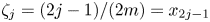 $\zeta _j=(2j-1)/(2m)=x_{2j-1}$, as illustrated in Appendix B. From the expression
 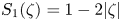 $S_1(\zeta )=1-2|\zeta |$ for
  $|\zeta |\le 1$, for
  $k=1,\ldots ,m$, we obtain
 \begin{align}
-f_{2k-3}+2f_{2k-1}-f_{2k+1} &=\sum_{j=1}^m
a_j[{-}S_1(\zeta_{k-1}-\zeta_j)+2S_1(\zeta_k-\zeta_j)-
S_1(\zeta_{k+1}-\zeta_j)] \nonumber\\ &=2\sum_{j=1}^m
a_j[|\zeta_{k-1}-\zeta_j|-2|\zeta_k-\zeta_j|+
|\zeta_{k+1}-\zeta_j|]\nonumber\\
&
=2a_k[|\zeta_{k-1}-\zeta_k|+|\zeta_{k+1}-\zeta_j|]
=\dfrac{4}{m}a_k.
\end{align}
\begin{align}
-f_{2k-3}+2f_{2k-1}-f_{2k+1} &=\sum_{j=1}^m
a_j[{-}S_1(\zeta_{k-1}-\zeta_j)+2S_1(\zeta_k-\zeta_j)-
S_1(\zeta_{k+1}-\zeta_j)] \nonumber\\ &=2\sum_{j=1}^m
a_j[|\zeta_{k-1}-\zeta_j|-2|\zeta_k-\zeta_j|+
|\zeta_{k+1}-\zeta_j|]\nonumber\\
&
=2a_k[|\zeta_{k-1}-\zeta_k|+|\zeta_{k+1}-\zeta_j|]
=\dfrac{4}{m}a_k.
\end{align}
For  $k=1$ and
  $m$, we use the symmetries
  $f_{-1}=-f_1$ and
 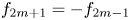 $f_{2m+1}=-f_{2m-1}$ to get the relations
 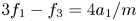 $3f_1-f_3=4a_1/m$ and
  $-f_{2m-3}+3f_{2m-1}=4a_m/m$. Thus,
 \begin{equation}
\renewcommand{\arraystretch}{1}
\left[\begin{array}{@{}ccccc@{}} 3 & -1 & & \\-1 & 2 & -1\\
& \ddots & \ddots & \ddots & \\ & & -1 & 2 & -1\\ & & & -1
& 3 \end{array}\right]
\begin{bmatrix}f_1\\f_3\\\vdots\\f_{2m-3}\\\,f_{2m-1}\end{bmatrix}
=\frac{4}{m}\begin{bmatrix}a_1\\a_2\\\vdots\\a_{m-1}\\a_m\end{bmatrix}.
\end{equation}
\begin{equation}
\renewcommand{\arraystretch}{1}
\left[\begin{array}{@{}ccccc@{}} 3 & -1 & & \\-1 & 2 & -1\\
& \ddots & \ddots & \ddots & \\ & & -1 & 2 & -1\\ & & & -1
& 3 \end{array}\right]
\begin{bmatrix}f_1\\f_3\\\vdots\\f_{2m-3}\\\,f_{2m-1}\end{bmatrix}
=\frac{4}{m}\begin{bmatrix}a_1\\a_2\\\vdots\\a_{m-1}\\a_m\end{bmatrix}.
\end{equation}
The symmetry  $f_{2m-k}=f_k$ for
 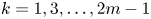 $k=1,3,\ldots ,2m-1$ implies that
  $a_{m-j}=a_j$ for
  $j=1,\ldots ,m-1$. It also makes it possible to halve the size of (E2) by only considering the first
  $m'=\lceil m/2\rceil$ coefficients, i.e.
 \begin{equation} \renewcommand{\arraystretch}{1}\left[\begin{array}{@{}ccccc@{}} 3 & -1 & & \\-1 & 2 & -1\\ & \ddots & \ddots & \ddots & \\ & & -1 & 2 & -1\\ & & & -2 & 2 \end{array}\right] \begin{bmatrix}f_1\\f_3\\\vdots\\f_{2m'-3}\\\,f_{2m'-1}\end{bmatrix} =\dfrac{4}{m}\begin{bmatrix}a_1\\a_2\\\vdots\\a_{m'-1}\\a_{m'}\end{bmatrix}. \end{equation}
The matrices in (E2) and (E3) play a fundamental role in the theory of discrete sine transforms, introduced as alternatives to the discrete Fourier transform for data with specific symmetries (Britanak et al. (Reference Britanak, Yip and Rao2007), page 36). For the example with  $m=11$ and
  $n=4$ used in Appendix B, we obtain
  $m'=6$ and
 \begin{align}
\renewcommand{\arraystretch}{1}
\begin{bmatrix}a_1\\a_2\\a_3\\a_4\\a_5\\a_6\end{bmatrix}
&=\dfrac{11}{4} \left[\begin{array}{@{}cccccc@{}} 3 & -1 & &
& \\-1 & 2 & -1\\ & -1 & 2 & -1 & & \\ & & -1 & 2 & -1 & \\
& & & -1 & 2 & -1\\ & & & & -2 & 2 \end{array}\right]
\dfrac{1}{22}\begin{bmatrix}5\\11\\13\\11\\5\\3\end{bmatrix} =\dfrac{1}{2}
\left[\begin{array}{@{}r@{}}1\\1\\1\\1\\-1\\-1\end{array}\right], \nonumber\\
\begin{bmatrix}a_7\\a_8\\a_9\\a_{10}\\a_{11}\end{bmatrix}
& =\begin{bmatrix}a_5\\a_4\\a_3\\a_2\\a_1\end{bmatrix}
=\dfrac{1}{2}\left[\begin{array}{@{}r@{}}-1\\1\\1\\1\\1\end{array}\right].
\end{align}
\begin{align}
\renewcommand{\arraystretch}{1}
\begin{bmatrix}a_1\\a_2\\a_3\\a_4\\a_5\\a_6\end{bmatrix}
&=\dfrac{11}{4} \left[\begin{array}{@{}cccccc@{}} 3 & -1 & &
& \\-1 & 2 & -1\\ & -1 & 2 & -1 & & \\ & & -1 & 2 & -1 & \\
& & & -1 & 2 & -1\\ & & & & -2 & 2 \end{array}\right]
\dfrac{1}{22}\begin{bmatrix}5\\11\\13\\11\\5\\3\end{bmatrix} =\dfrac{1}{2}
\left[\begin{array}{@{}r@{}}1\\1\\1\\1\\-1\\-1\end{array}\right], \nonumber\\
\begin{bmatrix}a_7\\a_8\\a_9\\a_{10}\\a_{11}\end{bmatrix}
& =\begin{bmatrix}a_5\\a_4\\a_3\\a_2\\a_1\end{bmatrix}
=\dfrac{1}{2}\left[\begin{array}{@{}r@{}}-1\\1\\1\\1\\1\end{array}\right].
\end{align}
The fact that  $a_j=\pm 0.5$ can be verified to hold for any
  $m$ and
  $n$ with opposite parities. The
  $\pm$ sign pattern is, in view of (E1), directly connected to the convexity of
  $f$, but its dependence on
  $j$ and
  $n$ for a fixed
  $m$ is not immediately obvious. Figure 23 illustrates the patterns when
  $m=11$. For the case
 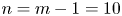 $n=m-1=10$ considered in Appendix C,
  $a_j=+0.5$ for all
  $j$. This remains true for other values of
  $m$. In particular,
 \begin{align}
\frac{2}{m}f_{1-1/m}(\zeta) =\frac{1}{m}\sum_{j=1}^m
S_1(\zeta-\zeta_j) \xrightarrow
[\substack{\text{midpoint}\\\text{rule}}]
{m\to\infty}\int_0^1 S_1(\zeta-x){\textrm{d}\kern0.05em x}
=\int_{\zeta-1}^\zeta S_1(x){\textrm{d}\kern0.05em x}=2\zeta(1-\zeta) \end{align}
\begin{align}
\frac{2}{m}f_{1-1/m}(\zeta) =\frac{1}{m}\sum_{j=1}^m
S_1(\zeta-\zeta_j) \xrightarrow
[\substack{\text{midpoint}\\\text{rule}}]
{m\to\infty}\int_0^1 S_1(\zeta-x){\textrm{d}\kern0.05em x}
=\int_{\zeta-1}^\zeta S_1(x){\textrm{d}\kern0.05em x}=2\zeta(1-\zeta) \end{align}
for  $0\le \zeta \le 1$ shows that
  $f_{1-1/m}(\zeta )\sim (m/4)4\zeta (1-\zeta )$ grows with
  $m$ as
  $m/4$ but its shape converges to
  $S_2(\zeta -0.5)$ from figure 10, providing an alternate proof of (4.20).

Figure 23. Signs of coefficients  $a_j$ for
  $m=11$ and
  $n$ and
  $j$ as indicated; blue is negative and red is positive.
Appendix F. Evaluation of the coefficients $s_k$ from (4.29)

The symmetry  $a_{m+1-j}=a_j$ for
  $j=1,\ldots ,m$ implies that
  $\sum _{j=1}^m a_j\cos ((2k+1){\rm \pi} \zeta _j)=0$. Thus,
 \begin{equation} is_k = \sum_{j=1}^m 2a_j\exp ({\textrm{i}(2k+1){\rm \pi}\zeta_j} ). \end{equation}
Replacing each exponential term of the sum associated with a factor  $2a_j=-1$ by
  $\textrm {e}^{-\textrm {i}{\rm \pi} \zeta _j}$ enables the interpretation of
  $is_k/m$ as the arithmetic mean of complex numbers on the unit circle and leads to the expression
 \begin{equation} s_k ={-}i\sum_{j=1}^m \exp ({\textrm{i}\,\text{sign}(a_j)(2k+1){\rm \pi}\zeta_j} ), \end{equation}
where  $0<\zeta _j=(2j-1){\rm \pi} /(2m)<{\rm \pi}$. Upon relabelling, the sum (F2) can be reformulated as a geometric sum of powers of
  $\xi =\exp [\textrm {i}(2k+1)(m-n){\rm \pi} /m]$. The process is illustrated in figure 24 for
  $m=11$,
  $n=4$ and
  $k=0$. We obtain, with
  $r=n/m$,
 \begin{align} s_k
&={-}\textrm{i}\sum_{\ell=1}^m \xi^{\ell-1/2}
={-}\textrm{i}\xi^{1/2}\frac{1-\xi^m}{1-\xi}
=\frac{2\textrm{i}}{\xi^{1/2}-\xi^{{-}1/2}}
=\csc\dfrac{(2k+1)}{2}\dfrac{(m-n)}{m}{\rm \pi} \nonumber\\
&=({-}1)^k\sec\dfrac{(2k+1)}{2}r{\rm \pi}.
\end{align}
\begin{align} s_k
&={-}\textrm{i}\sum_{\ell=1}^m \xi^{\ell-1/2}
={-}\textrm{i}\xi^{1/2}\frac{1-\xi^m}{1-\xi}
=\frac{2\textrm{i}}{\xi^{1/2}-\xi^{{-}1/2}}
=\csc\dfrac{(2k+1)}{2}\dfrac{(m-n)}{m}{\rm \pi} \nonumber\\
&=({-}1)^k\sec\dfrac{(2k+1)}{2}r{\rm \pi}.
\end{align}
Figure 24.  $(a)$ Signed complex numbers
  $2a_j\exp [i(2j-1){\rm \pi} /(2m)]$ for
  $j=1,\ldots ,m$ with
  $m=11$. The blue and red nodes correspond to
  $2a_j=-1$ and
  $2a_j=1$, respectively, for the
  $n=4$ case from figure 23. The nodes are labelled by the value of
  $j$ in the sum (F2).
  $(b)$ The blue terms
  $-\exp [i(2j-1){\rm \pi} /(2m)]$ (
 $\,j=5,6,7$) from
  $(a)$ are replaced by a red conjugate
  $\exp [-i(2j-1){\rm \pi} /(2m)]$ and the label in the nodes now represents the value of the counter
  $\ell$ in the sum (F3). Nodes with successive labels are obtained via multiplication by
  $\xi =\exp [i(m-n){\rm \pi} /m]$, corresponding to a counter-clockwise turn by an angle equal to
  $m-n=7$ nodes, starting with
  $\xi ^{1/2}$ (label 1).
Appendix G. The linear inviscid forced response as a superposition of $C^{\infty }$ elementary responses, (4.32), and its modal limit at resonance

Let  $\rho _k=(2k+1){\rm \pi}$ and
  $\lambda _k=\rho _k\,r/2$. The expansion (4.31) yields
 \begin{align}
f_r(x+rz)-f_r(x-rz) &=4\sum_{k\ge0}
\frac{({-}1)^k}{\rho_k^2}
\frac{\sin\rho_k(x+rz)-\sin\rho_k(x-rz)}{\cos\lambda_k}\nonumber\\
\quad &=8\sum_{k\ge0} \frac{({-}1)^k}{\rho_k^2} \frac{\cos\rho_k
x\,\sin\rho_k rz}{\cos\lambda_k},
\\[-2.1pc]\nonumber\end{align}
\begin{align}
f_r(x+rz)-f_r(x-rz) &=4\sum_{k\ge0}
\frac{({-}1)^k}{\rho_k^2}
\frac{\sin\rho_k(x+rz)-\sin\rho_k(x-rz)}{\cos\lambda_k}\nonumber\\
\quad &=8\sum_{k\ge0} \frac{({-}1)^k}{\rho_k^2} \frac{\cos\rho_k
x\,\sin\rho_k rz}{\cos\lambda_k},
\\[-2.1pc]\nonumber\end{align} \begin{align}
& 2x-f_r(x+rz)-f_r(x-rz)\nonumber\\
&\quad =
f_r(x+r/2)+f_r(x-r/2)-f_r(x+rz)-f_r(x-rz)\nonumber\\
&\quad =4\sum_{k\ge0}\frac{({-}1)^k}{\rho_k^2}
\frac{\sin\rho_k(x+r/2)+\sin\rho_k(x-r/2)
-\sin\rho_k(x+rz)-\sin\rho_k(x-rz)}{\cos\lambda_k}\nonumber\\
&\quad =8\sum_{k\ge0}\frac{({-}1)^k}{\rho_k^2}\sin\rho_k r x
\left(1-\frac{\cos\rho_k rz}{\cos\lambda_k}\right),
\end{align}
\begin{align}
& 2x-f_r(x+rz)-f_r(x-rz)\nonumber\\
&\quad =
f_r(x+r/2)+f_r(x-r/2)-f_r(x+rz)-f_r(x-rz)\nonumber\\
&\quad =4\sum_{k\ge0}\frac{({-}1)^k}{\rho_k^2}
\frac{\sin\rho_k(x+r/2)+\sin\rho_k(x-r/2)
-\sin\rho_k(x+rz)-\sin\rho_k(x-rz)}{\cos\lambda_k}\nonumber\\
&\quad =8\sum_{k\ge0}\frac{({-}1)^k}{\rho_k^2}\sin\rho_k r x
\left(1-\frac{\cos\rho_k rz}{\cos\lambda_k}\right),
\end{align}and
 \begin{align}
2rxz-F_r(x+rz)+F_r(x-rz)
&=r\int_0^z[2x-f_r(x+r\zeta)-f_r(x-r\zeta)]\,\textrm{d}\zeta
\nonumber\\ &=8\sum_{k\ge0}\frac{({-}1)^k}{\rho_k^2}
\sin\rho_kx \left(rz-\frac{\sin\rho_k
rz}{\rho_k\cos\lambda_k}\right).
\end{align}
\begin{align}
2rxz-F_r(x+rz)+F_r(x-rz)
&=r\int_0^z[2x-f_r(x+r\zeta)-f_r(x-r\zeta)]\,\textrm{d}\zeta
\nonumber\\ &=8\sum_{k\ge0}\frac{({-}1)^k}{\rho_k^2}
\sin\rho_kx \left(rz-\frac{\sin\rho_k
rz}{\rho_k\cos\lambda_k}\right).
\end{align}The response (4.15) of the linear inviscid forced system (4.1) can thus be written as a superposition
 \begin{equation} (u,w,p,\theta) =4\sum_{k\ge0} \frac{({-}1)^k}{\rho_k} (u_k,w_k,p_k,\theta_k) \end{equation}
of fields
 \begin{equation}
\left. \begin{aligned}
\begin{bmatrix}u_k\\w_k\end{bmatrix} &
=\frac{2c_r\sigma_r}{\rho_k} \begin{bmatrix}
\dfrac{r\cos\rho_kx \sin\rho_k rz}{\cos\lambda_k} \\
\sin\rho_kx \left(1-\dfrac{\cos\rho_k
rz}{\cos\lambda_k}\right) \end{bmatrix}\cos\sigma_rt \\ &
={-}\frac{\alpha}{\sigma_r} \begin{bmatrix}
\dfrac{\cos\rho_kx}{\cos\lambda_k}\dfrac{\sin\rho_k
rz}{\rho_k r},\\ \dfrac{1}{r^2}\dfrac{\sin\rho_kx}{\rho_k}
\left(1-\dfrac{\cos\rho_k rz}{\cos\lambda_k}\right)
\end{bmatrix}\cos\sigma_rt,\\
\begin{bmatrix}p_k\\\theta_k\end{bmatrix} &
={-}\frac{2c_r}{\rho_k} \begin{bmatrix}
\lambda_r\sin\rho_kx\left[rz-\dfrac{\sin\rho_k rz}
{\rho_k\cos\lambda_k}\right] \\
\sin\rho_kx\left[1-\dfrac{\cos\rho_k rz}
{\cos\lambda_k}\right]\end{bmatrix}\sin\sigma_rt\\ &
=\alpha\frac{\sin\rho_kx}{\rho_k} \begin{bmatrix}
z-\dfrac{1}{\cos\lambda_k}\dfrac{\sin\rho_k rz}{\rho_k r}
\\ \dfrac{1+r^2}{r^2} \left[1-\dfrac{\cos\rho_k
rz}{\cos\lambda_k}\right] \end{bmatrix}\sin\sigma_rt.
\end{aligned} \right\}
\end{equation}
\begin{equation}
\left. \begin{aligned}
\begin{bmatrix}u_k\\w_k\end{bmatrix} &
=\frac{2c_r\sigma_r}{\rho_k} \begin{bmatrix}
\dfrac{r\cos\rho_kx \sin\rho_k rz}{\cos\lambda_k} \\
\sin\rho_kx \left(1-\dfrac{\cos\rho_k
rz}{\cos\lambda_k}\right) \end{bmatrix}\cos\sigma_rt \\ &
={-}\frac{\alpha}{\sigma_r} \begin{bmatrix}
\dfrac{\cos\rho_kx}{\cos\lambda_k}\dfrac{\sin\rho_k
rz}{\rho_k r},\\ \dfrac{1}{r^2}\dfrac{\sin\rho_kx}{\rho_k}
\left(1-\dfrac{\cos\rho_k rz}{\cos\lambda_k}\right)
\end{bmatrix}\cos\sigma_rt,\\
\begin{bmatrix}p_k\\\theta_k\end{bmatrix} &
={-}\frac{2c_r}{\rho_k} \begin{bmatrix}
\lambda_r\sin\rho_kx\left[rz-\dfrac{\sin\rho_k rz}
{\rho_k\cos\lambda_k}\right] \\
\sin\rho_kx\left[1-\dfrac{\cos\rho_k rz}
{\cos\lambda_k}\right]\end{bmatrix}\sin\sigma_rt\\ &
=\alpha\frac{\sin\rho_kx}{\rho_k} \begin{bmatrix}
z-\dfrac{1}{\cos\lambda_k}\dfrac{\sin\rho_k rz}{\rho_k r}
\\ \dfrac{1+r^2}{r^2} \left[1-\dfrac{\cos\rho_k
rz}{\cos\lambda_k}\right] \end{bmatrix}\sin\sigma_rt.
\end{aligned} \right\}
\end{equation}
The fields  $(u_k,w_k,p_k,\theta _k)$ can be verified to satisfy the forced linear system (4.33) as well as the boundary conditions
  $u_k=\partial _x\theta _k=0$ at
  $x={\pm }0.5$, and
  $w_k=\theta _k=0$ at
  $z={\pm }0.5$. The resulting vorticity field
 \begin{equation} \eta_k=\partial_zu_k-\partial_xw_k =\frac{\alpha}{r^2\sigma_r}\cos\rho_k x \left[1-(1+r^2)\frac{\cos\rho_k rz}{\cos\lambda_k}\right]\cos\sigma_rt \end{equation}
is also used to evaluate the vorticity of partial sums of the series (4.32) in figure 13. The associated streamfunction
 \begin{equation} \psi_k ={-}\frac{\alpha}{\sigma_r} \frac{\cos\rho_k x}{(\rho_k r)^2} \left[1-\dfrac{\cos\rho_k rz}{\cos\lambda_k}\right]\cos\sigma_rt \end{equation}
vanishes at all boundaries of the cavity. Its  $\rho _k^{-2}$ dependence on
  $k$ makes the series (4.32) converge fast for the overall streamfunction
  $\psi$ from (4.8).
The limit of (G5) as  $r\to r^*=n/m$, with
  $m$ and
  $n$ both odd and
  $m\wedge n=1$ (prime with each other), can be taken for values of
  $k$ such that
  $\cos \lambda ^*_k=0$, where
  $\lambda ^*_k=\rho _kr^*/2$. These are the sole contributors, at the limit, to the overall series (4.32). In this case,
  $(2k+1)r^*$ is an odd integer. Since
  $m\wedge n=1$,
  $2k+1=(2\ell +1)m$ for
  $\ell \in \mathbb {N}$. Consequently,
  $\rho _kr^*/2=2{\rm \pi} \ell (n-1)/2+(\ell +(n-1)/2){\rm \pi} +{\rm \pi} /2$ and
 \begin{align} \cos\lambda_k =\cos[\lambda^*_k+(\lambda_k-\lambda^*_k)] ={-}\sin\lambda^*_k \sin(\lambda_k-\lambda^*_k) \approx{-}({-}1)^{\ell+(n-1)/2}\, (\lambda_k-\lambda^*_k). \end{align}
Thus, 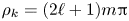 $\rho _k=(2\ell +1)m{\rm \pi}$,
 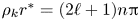 $\rho _kr^*=(2\ell +1)n{\rm \pi}$, and as
  $r\to r^*$,
 \begin{align}
\begin{bmatrix}u_k\\
w_k\end{bmatrix}
&\approx{-}\frac{\alpha}{\cos\lambda_k}
\dfrac{1}{\rho_k{r^*}^2\sigma_{r^*}} \begin{bmatrix}
r^*\cos\rho_kx\sin\rho_k r^*z \\ -\sin\rho_kx \cos\rho_k
r^*z \end{bmatrix} \cos\sigma_{r^*}t \nonumber\\
&\approx\gamma_k\sigma_{r^*} \begin{bmatrix}
r^*\cos(2\ell+1)m{\rm \pi} x \sin(2\ell+1)n{\rm \pi} z \\
-\sin(2\ell+1)m{\rm \pi} x \cos(2\ell+1)n{\rm \pi} z, \end{bmatrix}
\cos\sigma_{r^*}t,
\end{align}
\begin{align}
\begin{bmatrix}u_k\\
w_k\end{bmatrix}
&\approx{-}\frac{\alpha}{\cos\lambda_k}
\dfrac{1}{\rho_k{r^*}^2\sigma_{r^*}} \begin{bmatrix}
r^*\cos\rho_kx\sin\rho_k r^*z \\ -\sin\rho_kx \cos\rho_k
r^*z \end{bmatrix} \cos\sigma_{r^*}t \nonumber\\
&\approx\gamma_k\sigma_{r^*} \begin{bmatrix}
r^*\cos(2\ell+1)m{\rm \pi} x \sin(2\ell+1)n{\rm \pi} z \\
-\sin(2\ell+1)m{\rm \pi} x \cos(2\ell+1)n{\rm \pi} z, \end{bmatrix}
\cos\sigma_{r^*}t,
\end{align} \begin{align}
\begin{bmatrix}
p_k\\\theta_k\end{bmatrix}
&\approx{-}\frac{\alpha}{\cos\lambda_k}
\frac{\sin\rho_kx}{\rho_k {r^*}^2} \begin{bmatrix}
\dfrac{r^*}{\rho_k} \sin\rho_k r^*z \\
(1+{r^*}^2)\cos\rho_k r^*z \end{bmatrix} \sin\sigma_{r^*}t \nonumber\\
&\approx\gamma_k
\begin{bmatrix} \dfrac{r^*\sigma_{r^*}^2}{(2\ell+1)m{\rm \pi}}
\sin(2\ell+1)m{\rm \pi} x \sin(2\ell+1)n{\rm \pi} z \\
\sin(2\ell+1)m{\rm \pi} x \cos(2\ell+1)n{\rm \pi} z
\end{bmatrix} \sin\sigma_{r^*}t,
\end{align}
\begin{align}
\begin{bmatrix}
p_k\\\theta_k\end{bmatrix}
&\approx{-}\frac{\alpha}{\cos\lambda_k}
\frac{\sin\rho_kx}{\rho_k {r^*}^2} \begin{bmatrix}
\dfrac{r^*}{\rho_k} \sin\rho_k r^*z \\
(1+{r^*}^2)\cos\rho_k r^*z \end{bmatrix} \sin\sigma_{r^*}t \nonumber\\
&\approx\gamma_k
\begin{bmatrix} \dfrac{r^*\sigma_{r^*}^2}{(2\ell+1)m{\rm \pi}}
\sin(2\ell+1)m{\rm \pi} x \sin(2\ell+1)n{\rm \pi} z \\
\sin(2\ell+1)m{\rm \pi} x \cos(2\ell+1)n{\rm \pi} z
\end{bmatrix} \sin\sigma_{r^*}t,
\end{align}where
 \begin{equation} \gamma_k = \frac{\alpha}{r-r^*} \frac{2({-}1)^{\ell+(n-1)/2}}{\rho_k^2 {r^*}^2\sigma_{r^*}^2} =\frac{\alpha}{r-r^*} \frac{2({-}1)^{(n-1)/2}}{{\rm \pi}^2} \left(\frac{1}{m^2}+\frac{1}{n^2}\right)\frac{({-}1)^\ell}{(2\ell+1)^2}. \end{equation}
 The forced responses  $R_{f_k}\approx \gamma _k I_k$, with components given by (G9) that are scaled versions of those in (4.25) of
 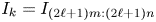 $I_k=I_{(2\ell +1)m:(2\ell +1)n}$, combine into the infinite sum (4.32),
 \begin{align} R_f
&\approx \frac{4}{\rm \pi}\sum_{k\ge0} \frac{({-}1)^k}{2k+1}
\gamma_k I_k \nonumber\\ &=\frac{\alpha}{r-r^*}
\frac{8({-}1)^{(n-1)/2}}{{\rm \pi}^3}
\left(\frac{1}{m^2}+\frac{1}{n^2}\right) \sum_{\ell\ge0}
\frac{({-}1)^{\ell m +(m-1)/2}}{(2\ell+1)m}
\frac{({-}1)^\ell}{(2\ell+1)^2} I_{(2\ell+1)m:(2\ell+1)n}
\nonumber\\
&=\mu_{r^*} \sum_{\ell\ge0}
\frac{1}{(2\ell+1)^3} I_{(2\ell+1)m:(2\ell+1)n},
\end{align}
\begin{align} R_f
&\approx \frac{4}{\rm \pi}\sum_{k\ge0} \frac{({-}1)^k}{2k+1}
\gamma_k I_k \nonumber\\ &=\frac{\alpha}{r-r^*}
\frac{8({-}1)^{(n-1)/2}}{{\rm \pi}^3}
\left(\frac{1}{m^2}+\frac{1}{n^2}\right) \sum_{\ell\ge0}
\frac{({-}1)^{\ell m +(m-1)/2}}{(2\ell+1)m}
\frac{({-}1)^\ell}{(2\ell+1)^2} I_{(2\ell+1)m:(2\ell+1)n}
\nonumber\\
&=\mu_{r^*} \sum_{\ell\ge0}
\frac{1}{(2\ell+1)^3} I_{(2\ell+1)m:(2\ell+1)n},
\end{align}
using the fact that  $\ell (m+1)$ is an even integer, with
 \begin{equation} \mu_{r^*}(r)={-}\frac{8}{{\rm \pi}^3}\frac{({-}1)^{(m+n)/2}}{m} \left(\frac{1}{m^2}+\frac{1}{n^2}\right)\frac{\alpha}{r-r^*}. \end{equation}
Note that 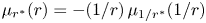 $\mu _{r^*}(r)=-(1/r)\,\mu _{1/r^*}(1/r)$, i.e. the resonant response is stronger for
  $r\approx r^*<1$ (
 $\omega ^2>0.5$), which is consistent with the response diagram in figure 2
 $(a)$.
The limiting process  $r\to r^*$ carried out directly on
  $f_r$ from (4.31), using (G8), yields
 \begin{align}
f_r(\zeta) &\approx{-}\frac{4}{{\rm \pi}^2}\sum_{\ell\ge0}
\frac{({-}1)^{\ell m+(m-1)/2}}{(2\ell+1)^2\, m^2}
\frac{\sin(2\ell+1)m{\rm \pi}\zeta} {({-}1)^{\ell+(n-1)/2}
(2\ell+1)\,m{\rm \pi}\,(r-r*)/2}\nonumber\\
&={-}\frac{({-}1)^{(m+n)/2}}{4m^3 (r-r^*)}
\left(\frac{32}{{\rm \pi}^3}\right) \sum_{\ell\ge0}
\frac{\sin(2\ell+1)m{\rm \pi}\zeta}{(2\ell+1)^3}
={-}\frac{({-}1)^{(m+n)/2}}{4m^3 (r-r^*)} S_2(m\zeta-0.5),
\end{align}
\begin{align}
f_r(\zeta) &\approx{-}\frac{4}{{\rm \pi}^2}\sum_{\ell\ge0}
\frac{({-}1)^{\ell m+(m-1)/2}}{(2\ell+1)^2\, m^2}
\frac{\sin(2\ell+1)m{\rm \pi}\zeta} {({-}1)^{\ell+(n-1)/2}
(2\ell+1)\,m{\rm \pi}\,(r-r*)/2}\nonumber\\
&={-}\frac{({-}1)^{(m+n)/2}}{4m^3 (r-r^*)}
\left(\frac{32}{{\rm \pi}^3}\right) \sum_{\ell\ge0}
\frac{\sin(2\ell+1)m{\rm \pi}\zeta}{(2\ell+1)^3}
={-}\frac{({-}1)^{(m+n)/2}}{4m^3 (r-r^*)} S_2(m\zeta-0.5),
\end{align}
where  $S_2(\cdot -0.5)$ is the 1-antiperiodic quadratic spline shown in figure 10
 $(b)$. For the case
  $m=1$, one immediately recovers (4.20). Note that
  $m$ in (4.20) is related to
  $r=1-1/m$, while
  $m$ here is related to the limiting value
  $r^*=n/m$. Moreover, the scaling of (G13) reduces, in the case
  $n=1$, to the factor
  $m/4$, with
  $m$ as in (G13), already obtained in Appendix C.
Appendix H. Inviscid estimate of mean enstrophy
The inviscid enstrophy is determined by substituting the expression (G7) into the series (G4). The orthogonality
 \begin{equation} \int_{{-}0.5}^{0.5} \cos\rho_kx \cos\rho_\ell x\,\textrm{d}\kern0.06em x=0, \quad k\ne\ell, \end{equation}
implies that  $\{\eta _k\}_{k\ge 0}$ forms an orthogonal sequence with respect to the
 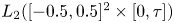 $L_2([-0.5,0.5]^2\times [0,\tau ])$ inner product. This yields
 \begin{align}
\langle\mathcal{E}\rangle_\tau &=\frac{1}{\tau}\int_0^\tau
\int_{{-}0.5}^{0.5}\int_{{-}0.5}^{0.5}
\left[4\sum_{k\ge0}({-}1)^k\frac{\eta_k}{\rho_k}\right]^{2}
\,\textrm{d}\kern0.06em x\,\textrm{d}z
=\frac{16}{\tau}\sum_{k\ge0}\frac{1}{\rho_k^{2}}
\int_0^\tau\int_{{-}0.5}^{0.5}\int_{{-}0.5}^{0.5}\eta_k^2\,
\textrm{d}\kern0.06em x\,\textrm{d}z \nonumber\\
&=\frac{16\alpha^2}{r^4\sigma_r^2}
\sum_{k\ge0}\frac{1}{\tau\rho_k^{2}} \int_0^\tau
\cos^2\sigma_rt\,\textrm{d}t \int_{{-}0.5}^{0.5}
\cos^2\rho_kx\,\textrm{d}\kern0.06em x\nonumber\\
&\quad\times
\int_{{-}0.5}^{0.5}\left[1-(1+r^2)\frac{\cos\rho_k
rz}{\cos\lambda_k}\right]^{2}\,\textrm{d}\kern0.06em x\,\textrm{d}z \nonumber\\
&=\frac{4\alpha^2}{r^4\sigma_r^2}
\sum_{k\ge0}\rho_k^{{-}2}
\left\{1-4(1+r^2)\frac{\sin(\lambda_k)/(\rho_k
r)}{\cos\lambda_k}+(1+r^2)^2
\frac{1+\sin(\rho_kr)/(\rho_kr)}{2\cos^2\lambda_k}\right\}\nonumber\\
&=\frac{\alpha^2}{r^2\sigma_r^2}\sum_{k\ge0}
\lambda_k^{{-}2}
\left\{1+\frac{1+r^2}{2}\left[(1+r^2)\sec^2\lambda_k
-(3-r^2)\frac{\tan\lambda_k}{\lambda_k}\right]\right\}.
\end{align}
\begin{align}
\langle\mathcal{E}\rangle_\tau &=\frac{1}{\tau}\int_0^\tau
\int_{{-}0.5}^{0.5}\int_{{-}0.5}^{0.5}
\left[4\sum_{k\ge0}({-}1)^k\frac{\eta_k}{\rho_k}\right]^{2}
\,\textrm{d}\kern0.06em x\,\textrm{d}z
=\frac{16}{\tau}\sum_{k\ge0}\frac{1}{\rho_k^{2}}
\int_0^\tau\int_{{-}0.5}^{0.5}\int_{{-}0.5}^{0.5}\eta_k^2\,
\textrm{d}\kern0.06em x\,\textrm{d}z \nonumber\\
&=\frac{16\alpha^2}{r^4\sigma_r^2}
\sum_{k\ge0}\frac{1}{\tau\rho_k^{2}} \int_0^\tau
\cos^2\sigma_rt\,\textrm{d}t \int_{{-}0.5}^{0.5}
\cos^2\rho_kx\,\textrm{d}\kern0.06em x\nonumber\\
&\quad\times
\int_{{-}0.5}^{0.5}\left[1-(1+r^2)\frac{\cos\rho_k
rz}{\cos\lambda_k}\right]^{2}\,\textrm{d}\kern0.06em x\,\textrm{d}z \nonumber\\
&=\frac{4\alpha^2}{r^4\sigma_r^2}
\sum_{k\ge0}\rho_k^{{-}2}
\left\{1-4(1+r^2)\frac{\sin(\lambda_k)/(\rho_k
r)}{\cos\lambda_k}+(1+r^2)^2
\frac{1+\sin(\rho_kr)/(\rho_kr)}{2\cos^2\lambda_k}\right\}\nonumber\\
&=\frac{\alpha^2}{r^2\sigma_r^2}\sum_{k\ge0}
\lambda_k^{{-}2}
\left\{1+\frac{1+r^2}{2}\left[(1+r^2)\sec^2\lambda_k
-(3-r^2)\frac{\tan\lambda_k}{\lambda_k}\right]\right\}.
\end{align}
Note that, for fixed  $k$, the term in the curly brackets is
  ${O}(r^4)$ as
  $r\to 0$ (
 $\omega =\sigma _r\to 1$).


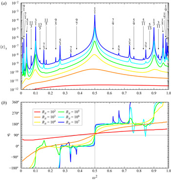


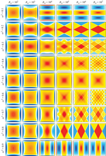


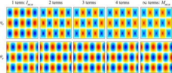


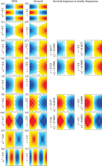


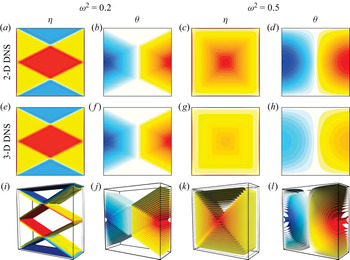


 Open access