3.1. Ornstein–Uhlenbeck process in one dimension

Consider the advection of a 1-D tracer by an Ornstein–Uhlenbeck (OU) process in a $2 {\rm \pi}$ periodic domain. The equations of motion are

(3.1)\begin{gather} {\rm d}\tilde{u}_\omega ={-} \tilde{u}_\omega \,{\rm d}t + \sqrt{2} \,{\rm d}W_\omega, \end{gather}

(3.2)\begin{gather}\partial_t \theta_\omega ={-}\tilde{u}_\omega \partial_x \theta_\omega + \kappa \partial_{xx} \theta_\omega + s(x), \end{gather}

where $s$ is a mean zero source, $\omega$ labels the ensemble member and we choose $\kappa = 0.01$ for the diffusivity constant. We shall calculate the turbulent diffusivity operator for this system in two different ways. The first will be by simulating the equations and the second will be by using numerical approximations of the conditional mean equations.

Since the flow field $u$ is independent of the spatial variable and the domain is periodic, we decompose the tracer equation using Fourier modes and calculate a diffusivity as a function of wavenumber $k$, wavenumber by wavenumber. Decomposing $\theta _\omega$ as

(3.3a,b)\begin{equation} \theta_\omega(x, t) = \sum_{n={-}\infty}^{\infty} \hat{\theta}^n_\omega(t) {\rm e}^{{\rm i} k_n x} \quad\text{and}\quad s(x) = \sum_{n={-}\infty}^{\infty} \hat{s}^n {\rm e}^{{\rm i} k_n x}, \end{equation}

where $k_n = n$, yields

(3.4)\begin{gather} {\rm d}\tilde{u}_\omega ={-} \tilde{u}_\omega \,{\rm d}t + \sqrt{2} \,{\rm d}W_\omega, \end{gather}

(3.5)\begin{gather}\frac{{\rm d}}{{\rm d}t} \hat{\theta}_\omega^n ={-}\tilde{u}_\omega {\rm i} k_n \hat{\theta}_\omega^n - \kappa k_n^2 \hat{\theta}_\omega^n + \hat{s}^n, \end{gather}

which are ordinary differential equations for each wavenumber $k_n$ with no coupling between wavenumbers. We define a ‘turbulent diffusivity’ on a wavenumber by wavenumber basis with

(3.6)\begin{equation} \kappa_T(k_n) ={-}\frac{\langle \tilde{u} \hat{\theta}^n \rangle}{\langle {\rm i} k_n \hat{\theta}^n \rangle}, \end{equation}

which is a flux divided by a gradient. A local diffusivity would be independent of wavenumber. Here the averaging operator, $\langle {\cdot } \rangle$, is an average over all ensemble members. This quantity is independent of the source wavenumber amplitude, $\hat {s}^n$, for non-zero sources and conventions for scaling the Fourier transform. With this observation in place, we take our source term to be $s(x) = \delta (x) - 1$ so that $\hat {s}^n = 1$ for all $n \neq 0$ and $\hat {s}^0 = 0$. We numerically simulate (3.1) and (3.2) in spectral space until a time $t=25$ using $10^6$ ensemble members and then perform the ensemble average at this fixed time. We have finished the description for the first method of calculation. We now move on to using the conditional mean equations directly.

The conditional mean equations recover the same result as the continuous ensemble mean. We show this through numerical discretization. The conditional mean equation version of (3.1) and (3.2) is

(3.7)\begin{gather} \partial_t \mathcal{P} = \partial_u\left( - \mathcal{P} + \partial_u \mathcal{P} \right), \end{gather}

(3.8)\begin{gather}\partial_t \varTheta ={-} u \partial_x \varTheta + \kappa \partial_{xx} \varTheta + \mathcal{P} s + \partial_u\left( - \varTheta + \partial_u \varTheta \right), \end{gather}

where $\varTheta = \varTheta (x, u, t)$ and $\mathcal {P} = \mathcal {P}(u, t)$. We make the observation

(3.9a,b)\begin{equation} \int_{ -\infty}^{\infty} \,{\rm d}u \varTheta = \langle \theta \rangle\quad \text{and} \quad \int_{-\infty}^{\infty} \,{\rm d}u u \varTheta = \langle \tilde{u} \theta \rangle. \end{equation}

To discretize the $u$ variable, we invoke a finite volume discretization by integrating with respect to $N = N'+1$ control volumes $\varOmega _m = [(2m - 1 - N') / \sqrt {N'},(2m + 1 - N') / \sqrt {N'}]$ for $m = 0,\ldots, N'$, a procedure which is detailed in Appendix C.2. The result is

(3.10)\begin{gather} \partial_t \mathcal{P}_m = \sum_{m'} \mathcal{Q}_{m m'} \mathcal{P}_{m'}, \end{gather}

(3.11)\begin{gather}\partial_t \varTheta_m ={-} u_m \partial_x \hat{\varTheta}_m + \kappa \partial_{xx} \hat{\varTheta}^n_m + \mathcal{P}_m s + \sum_{m'} \mathcal{Q}_{m m'} \varTheta_{m'}, \end{gather}

where

(3.12a–c)\begin{align} \int_{\varOmega_m} \,{\rm d}u \varTheta = \varTheta_m , \quad \int_{\varOmega_m} \,{\rm d}u \mathcal{P}= \mathcal{P}_m ,\quad u_m = \frac{2}{\sqrt{N'}}(m - N'/2),\quad \int_{\varOmega_m} \,{\rm d}u u \varTheta \approx u_m \varTheta_m , \end{align}

and $\mathcal {Q}_{mm'} = ( -N' \delta _{mm'} + m' \delta _{(m+1)m'} + (N'-m')\delta _{(m-1)m'} )/2$ and $m = 0 ,\ldots, N'$. This approximation is the same as that used by Hagan et al. (Reference Hagan, Doering and Levermore1989) to represent the Ornstein–Uhlenbeck process by Markov jump processes, but now justified as a finite volume discretization. Observe that for $N = 2$, we have a dichotomous velocity process

(3.13)\begin{gather} \partial_t \mathcal{P}_1 ={-} 0.5 \mathcal{P}_{1} + 0.5 \mathcal{P}_2, \end{gather}

(3.14)\begin{gather}\partial_t \mathcal{P}_2 ={-} 0.5 \mathcal{P}_{2} + 0.5 \mathcal{P}_1, \end{gather}

(3.15)\begin{gather}\partial_t \varTheta_1 ={-} \partial_x \hat{\varTheta}_1 + \kappa \partial_{xx} \varTheta_1 + \mathcal{P}_1 s - 0.5 \varTheta_{1} + 0.5 \varTheta_2, \end{gather}

(3.16)\begin{gather}\partial_t \varTheta_2 = \partial_x \hat{\varTheta}_2 + \kappa \partial_{xx} \varTheta_1 + \mathcal{P}_2 s - 0.5 \varTheta_{2} + 0.5 \varTheta_1 \end{gather}

and for $N=3$, we have a generalization

(3.17)\begin{gather} \partial_t \mathcal{P}_1 ={-} \mathcal{P}_{1} + 0.5 \mathcal{P}_2, \end{gather}

(3.18)\begin{gather}\partial_t \mathcal{P}_2 ={-} \mathcal{P}_{2} + \mathcal{P}_1 + \mathcal{P}_3, \end{gather}

(3.19)\begin{gather}\partial_t \mathcal{P}_3 ={-} \mathcal{P}_{3} + 0.5 \mathcal{P}_2, \end{gather}

(3.20)\begin{gather}\partial_t \varTheta_1 ={-}\sqrt{2} \partial_x \hat{\varTheta}_1 + \kappa \partial_{xx} \varTheta_1 + \mathcal{P}_1 s - \varTheta_{1} + 0.5 \varTheta_2, \end{gather}

(3.21)\begin{gather}\partial_t \varTheta_2 = 0 \partial_x \hat{\varTheta}_2 + \kappa \partial_{xx} \varTheta_1 + \mathcal{P}_2 s - \varTheta_{2} + \varTheta_1 + \varTheta_3, \end{gather}

(3.22)\begin{gather}\partial_t \varTheta_3 = \sqrt{2} \partial_x \hat{\varTheta}_3 + \kappa \partial_{xx} \varTheta_1 + \mathcal{P}_3 s - \varTheta_{3} + 0.5 \varTheta_2, \end{gather}

similar to the models of Davis et al. (Reference Davis, Flierl, Wiebe and Franks1991) and Ferrari, Manfroi & Young (Reference Ferrari, Manfroi and Young2001). The presence of an evolution equation for $\mathcal {P}_n$ accounts for statistically non-stationary states of the flow field. Alternative discretizations are possible. For example, using a spectral discretization for the $u$ variable via Hermite polynomials converges to the continuous system at a faster rate; however, the resulting discrete system no longer has an interpretation as a Markov jump process for three or more state variables.

Next, taking the Fourier transform in $x$ yields

(3.23)\begin{equation} \frac{{\rm d}}{{\rm d}t} \hat{\varTheta}^n_m ={-} u_m {\rm i} k_n \hat{\varTheta}^n_m - \kappa k_n^2 \hat{\varTheta}^n_m + \sum_{m'} \mathcal{Q}_{m m'} \hat{\varTheta}^n_{m'}. \end{equation}

We solve for the steady-state solution

(3.24)\begin{gather} 0 = \sum_{m'} \mathcal{Q}_{m m'} \mathcal{P}_{m'}, \end{gather}

(3.25)\begin{gather}0 ={-} u_m {\rm i} k_n \hat{\varTheta}^n_m - \kappa k_n^2 \hat{\varTheta}^n_m + \mathcal{P}_m \hat{s}^n + \sum_{m'} \mathcal{Q}_{m m'} \hat{\varTheta}^n_{m'} \end{gather}

and then compute

(3.26) \begin{equation} \kappa_E(k_n) ={-}\frac{\displaystyle\sum_m u_m \hat{\varTheta}_m^n}{\displaystyle \sum_m {\rm i} k_n \hat{\varTheta}_m^n } \Rightarrow -\frac{\displaystyle\int_{-\infty}^\infty \,{\rm d}u \hat{\varTheta}^n u }{\displaystyle\int_{-\infty}^\infty \,{\rm d}u ({\rm i} k_n \hat{\varTheta}^n) } \end{equation}

for various choices of discrete states. The calculations in the numerator and denominator are equivalent to ensemble averages.

We compare the two methods of calculation in figure 1. We see that increasing the number of states from $N=2$ to $N=15$ yields, for each wavenumber, ensemble averages similar to those of the Ornstein–Uhlenbeck process. The explicit formula for $N=3$ is given in the next section. We stop at $N = 15$ states since all wavenumbers in the plot are within 1 % of one another. The $n=0$ wavenumber is plotted for convenience as well and, in the case of the present process, also happens to correspond to the velocity autocorrelation. The correspondence of all velocity states (including the Ornstein–Uhlenbeck process) at wavenumber $k_n=0$ is particular to this system and is not a feature that holds in general. The ‘large scale limit’, corresponding to wavenumber $k_n = 0$, can often be considered an appropriate local diffusivity definition.

Figure 1. Wavenumber diffusivities. We show the turbulent diffusivity estimate as a function of wavenumber. Here we see that different wavenumbers, or equivalently length scales, produce different estimates of the turbulent diffusivity. Furthermore, we show that the different N-state approximations yield an increasingly better approximation to the Ornstein–Uhlenbeck empirical estimate.

Although we use the finite volume discretization of velocity states as approximations to the Ornstein–Uhlenbeck process, they also constitute a realizable stochastic process in the form of a Markov jump process. Thus, each finite state case can be simulated from whence the turbulent diffusivity estimate in figure 1 is exact rather than an approximation. We choose a particular example with $N=3$ in the following section.

Furthermore, each wavenumber $k_n$ yields a different estimate of the turbulent diffusivity. In particular, the decrease of turbulent diffusivity as a function of wavenumber implies non-locality. Choosing a forcing that is purely sinusoidal of a given mode would yield different estimates of turbulent fluxes. For example, forcing with $s(x) = \sin (x)$ would yield a diffusivity estimate of $\kappa _T(1) \approx 0.58$, whereas forcing with $s(x) = \sin (2x)$ would yield a diffusivity estimate of $\kappa _T(2) \approx 0.34$, as implied by figure 1.

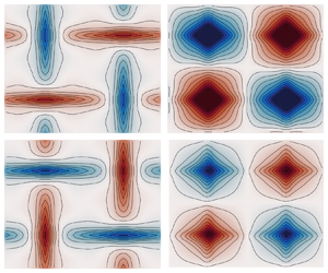
In the present case, the inverse Fourier transform of the turbulent diffusivity yields the turbulent diffusivity operator in real space. Since products in wavenumber space are circular convolutions in real space, we naturally guarantee the translation invariance of the kernel for the present case. The turbulent diffusivity kernels are shown in figure 2. Thus, the equation for the ensemble mean is

(3.27)\begin{equation} -\partial_x \left( \mathcal{K} * \partial_x \langle \theta \rangle + \kappa \partial_x \langle \theta \rangle \right) = s(x), \end{equation}

where $*$ is a circular convolution with the kernel in figure 2.

Figure 2. Kernels for N-state systems. Here we show the turbulent diffusivity kernels for several approximations of the Ornstein–Uhlenbeck diffusivity kernel. We compare all kernels to the $N = 15$ state kernel, which is a good approximation to the OU process kernel. We see that the width of the kernel is comparable to the domain. The non-locality of the kernel is a consequence of the turbulent diffusivity estimate differing on a wavenumber per wavenumber basis.

To illustrate the action of a non-local operator, we show the implied flux for a gradient that is presumed to have the functional form

(3.28)\begin{equation} \partial_x \langle \theta \rangle = \exp( - 2 (x- {\rm \pi})^2 ) - \exp({-}10(x- 9 {\rm \pi}/ 8)^2 ). \end{equation}

The flux computed from the convolution with the $N=15$ state kernel

(3.29)\begin{equation} \langle \tilde{u} \theta \rangle ={-}\mathcal{K} * \partial_x \langle \theta \rangle \end{equation}

is shown in figure 3. Even though the gradient changes sign, we see that the flux remains purely negative, i.e. the flux is up-gradient at particular points of the domain. Furthermore, the figure 3(b) does not resemble a straight line through the origin, as would be the case for a local diffusivity. The red portion highlights the ‘up-gradient’ part of the flux-gradient relation. We point out these features to illustrate the limitations of a purely local flux-gradient relationship.

Figure 3. Flux prediction from the kernel. Given the ensemble mean gradient (green), we convolve with the $N=15$ state kernel to get the flux (yellow) in panel (a). We see that the gradient changes sign while the flux always remains negative. To further illustrate the effect of non-locality, we show flux versus gradient in panel (b). The blue regions are down-gradient and the red regions are up-gradient. A local diffusivity estimate would be a straight line through the origin, whose slope determines the diffusivity constant.

This section focused on a flow field with a simple spatial and temporal structure. In the next section, we derive the turbulent diffusivity operator for a flow with arbitrary spatial structure but with a simple statistical temporal structure: a three-state velocity field whose amplitude is an approximation to the Ornstein–Uhlenbeck process.

3.2. A generalized three-state system with a 2-D example

For this example, we consider a Markov process that transitions between three incompressible states $\boldsymbol {u}_1(\boldsymbol {x}) = \boldsymbol {u}(\boldsymbol {x})$, $\boldsymbol {u}_2(\boldsymbol {x}) = 0$ and $\boldsymbol {u}_3(\boldsymbol {x}) = -\boldsymbol {u}(\boldsymbol {x})$. We use the three-state approximation to the Ornstein–Uhlenbeck process, in which case we let the generator be

(3.30)\begin{equation} \mathcal{Q} = \gamma \begin{bmatrix} -1 & 1/2 & 0 \\ 1 & -1 & 1 \\ 0 & 1/2 & -1 \end{bmatrix}, \end{equation}

where $\gamma > 0$. This generator implies that the flow field stays in each state for an exponentially distributed amount of time, with each state's rate parameter $\gamma$. Flow fields $\boldsymbol {u}_1$ and $\boldsymbol {u}_3$ always transition to state $\boldsymbol {u}_2$ and $\boldsymbol {u}_2$ transitions to either $\boldsymbol {u}_1$ or $\boldsymbol {u}_3$ with $50\,\%$ probability. This stochastic process is a generalization of the model considered in the previous section and the class of problems considered by Ferrari et al. (Reference Ferrari, Manfroi and Young2001) since the flow field can have spatial structure and is not limited to one dimension.

The three-state system is viewed as a reduced-order statistical model for any flow field that randomly switches between clockwise or counterclockwise advection, such as the numerical and experimental flows of Sugiyama et al. (Reference Sugiyama, Ni, Stevens, Chan, Zhou, Xi, Sun, Grossmann, Xia and Lohse2010). In their work, the numerical computations of 2-D Rayleigh–Bénard convection in a rectangular domain with no-slip boundary conditions along all walls yielded large-scale convection rolls that flipped orientation at random time intervals upon particular choices of Rayleigh and Prandtl numbers. In addition, they showed that the phenomenology could be observed in a laboratory experiment with a setup similar to that of Xia, Sun & Zhou (Reference Xia, Sun and Zhou2003). In general, we expect reducing the statistics of a flow to a continuous-time Markov process with discrete states to be useful and lead to tractable analysis in fluid flows characterized by distinct well-separated flow regimes with seemingly random transitions between behaviours. Consequently, a similar construction is possible for more complex three-dimensional flow fields, such as those of Brown & Ahlers (Reference Brown and Ahlers2007), or geophysical applications (Zhang, Zhang & Tian Reference Zhang, Zhang and Tian2022).

Proceeding with calculations, we note that the eigenvectors of the generator are

(3.31a–c)\begin{equation} \boldsymbol{v}^1 = \begin{bmatrix} 1/4 \\ 1/2 \\ 1/4 \end{bmatrix},\quad \boldsymbol{v}^2 = \begin{bmatrix} 1/2 \\ 0 \\ -1/2 \end{bmatrix} \quad \text{and}\quad \boldsymbol{v}^3 = \begin{bmatrix} 1/4 \\ -1/2 \\ 1/4 \end{bmatrix} \end{equation}

with respective eigenvalues $\lambda ^1 = 0$, $\lambda ^2 = - \gamma$ and $\lambda ^3 = - 2 \gamma$.

The statistically steady three-state manifestation of (2.13) and (2.14) is

(3.32)\begin{gather} \boldsymbol{\nabla} \boldsymbol{\cdot} \left( \boldsymbol{u} \varTheta_1 \right) = \kappa \Delta \varTheta_1 + s(\boldsymbol{x}) /4 - \gamma \varTheta_1 + \gamma \varTheta_2 / 2, \end{gather}

(3.33)\begin{gather}0 = \kappa \Delta \varTheta_2 + s(\boldsymbol{x})/2 - \gamma \varTheta_2 + \gamma \varTheta_1 + \gamma \varTheta_3, \end{gather}

(3.34)\begin{gather}- \boldsymbol{\nabla} \boldsymbol{\cdot} \left( \boldsymbol{u} \varTheta_3 \right) = \kappa \Delta \varTheta_3 + s(\boldsymbol{x})/4 - \gamma \varTheta_3 + \gamma \varTheta_2 / 2. \end{gather}

We define a transformation using the eigenvectors of the generator $\mathcal {Q}$,

(3.35)\begin{equation} \begin{bmatrix} 1/4 & 1/2 & 1/4 \\ 1/2 & 0 & -1/2 \\ 1/4 & -1/2 & 1/4 \end{bmatrix} \begin{bmatrix} \varphi_1 \\ \varphi_2 \\ \varphi_3 \end{bmatrix} = \begin{bmatrix} \varTheta_1 \\ \varTheta_2 \\ \varTheta_3 \end{bmatrix} \Leftrightarrow \begin{bmatrix} \varphi_1 \\ \varphi_2 \\ \varphi_3 \end{bmatrix} = \begin{bmatrix} 1 & 1 & 1 \\ 1 & 0 & -1 \\ 1 & -1 & 1 \end{bmatrix} \begin{bmatrix} \varTheta_1 \\ \varTheta_2 \\ \varTheta_3 \end{bmatrix} \end{equation}

resulting in the equations

(3.36)\begin{gather} \boldsymbol{\nabla} \boldsymbol{\cdot} \left(\boldsymbol{u} \varphi_2 \right) = \kappa \Delta \varphi_1 + s(\boldsymbol{x}), \end{gather}

(3.37)\begin{gather}\tfrac{1}{2} \boldsymbol{u}\boldsymbol{\cdot} \boldsymbol{\nabla} \varphi_1 + \tfrac{1}{2} \boldsymbol{u} \boldsymbol{\cdot} \boldsymbol{\nabla} \varphi_3 = \kappa \Delta \varphi_2 - \gamma \varphi_2, \end{gather}

(3.38)\begin{gather}\boldsymbol{u} \boldsymbol{\cdot} \boldsymbol{\nabla} \varphi_2 = \kappa \Delta \varphi_3 - 2 \gamma \varphi_3 . \end{gather}

We comment that $\varphi _1 = \langle \theta \rangle$, and that $\varphi _2$ and $\varphi _3$ are thought of as perturbation variables. Furthermore, the turbulent flux is $\langle \boldsymbol {\tilde {u}}' \theta ' \rangle = \boldsymbol {u} \varphi _2$. We eliminate dependence on the perturbation variables $\varphi _2$ and $\varphi _3$ by first solving for $\varphi _3$ in terms of $\varphi _2$,

(3.39)\begin{equation} \varphi_3 = \left(\kappa \Delta - 2 \gamma \right)^{{-}1} \boldsymbol{u} \boldsymbol{\cdot} \boldsymbol{\nabla} \varphi_2, \end{equation}

and then solving for $\varphi _2$ in terms of $\varphi _1$,

(3.40)\begin{equation} \varphi_2 = \left(\kappa \Delta -\gamma - \tfrac{1}{2}\boldsymbol{u} \boldsymbol{\cdot} \boldsymbol{\nabla} \left( \kappa \Delta -2 \gamma \right)^{{-}1} \boldsymbol{u} \boldsymbol{\cdot} \boldsymbol{\nabla} \right)^{{-}1}\tfrac{1}{2} \boldsymbol{u} \boldsymbol{\cdot} \boldsymbol{\nabla} \varphi_1. \end{equation}

And finally, we write our equation for the ensemble mean as

(3.41)\begin{equation} \boldsymbol{\nabla} \boldsymbol{\cdot} \left(\boldsymbol{u} \left(\kappa \Delta -\gamma - \tfrac{1}{2}\boldsymbol{u} \boldsymbol{\cdot} \boldsymbol{\nabla} \left( \kappa \Delta -2 \gamma \right)^{{-}1} \boldsymbol{u} \boldsymbol{\cdot} \boldsymbol{\nabla} \right)^{{-}1}\tfrac{1}{2} \boldsymbol{u} \boldsymbol{\cdot} \boldsymbol{\nabla} \langle \theta \rangle \right) = \kappa \Delta \langle \theta \rangle + s(\boldsymbol{x} ) \end{equation}

from whence we extract the turbulent diffusivity operator

(3.42)\begin{equation} \int \,{\rm d} \boldsymbol{x}' \mathcal{K}(\boldsymbol{x} | \boldsymbol{x}') \bullet{=} \boldsymbol{u} \left(\gamma-\kappa \Delta + \tfrac{1}{2}\boldsymbol{u} \boldsymbol{\cdot} \boldsymbol{\nabla} \left( \kappa \Delta -2 \gamma \right)^{{-}1} \boldsymbol{u} \boldsymbol{\cdot} \boldsymbol{\nabla} \right)^{{-}1}\tfrac{1}{2} \boldsymbol{u} . \end{equation}

We point out a few salient features of (3.42).

For large $\kappa$, we have

(3.43)\begin{align} \int \,{\rm d} \boldsymbol{x}' \mathcal{K}(\boldsymbol{x} | \boldsymbol{x}') \bullet \rightarrow \boldsymbol{u} \left(\gamma -\kappa \Delta \right)^{{-}1}\tfrac{1}{2} \boldsymbol{u} . \end{align}

The inverse Helmholtz operator, $(\gamma - \kappa \Delta )^{-1}$, damps high spatial frequency components of ensemble mean gradients. Thus, the operator's eigenvalues decrease as one examines increasingly fine-scale structure. Intuitively, as one examines a small-scale structure, the presence of diffusivity leads to lower turbulent fluxes, expressing that it is challenging to transport something that immediately diffuses.

A second observation pertains to the presence of the eigenvalue of the generator in the operator. If the flow field changes rapidly, transitioning between the disparate states, then $\gamma$ is large and one can expect the turbulent diffusivity to be local. In other words, the flow does not stay sufficiently long time near a coherent structure. More concretely, larger transition rates correspond to an enhanced locality in the turbulent diffusivity operator since, as $\gamma \rightarrow \infty$,

(3.44)\begin{equation} \int \,{\rm d} \boldsymbol{x}' \mathcal{K}(\boldsymbol{x} | \boldsymbol{x}') \bullet \rightarrow \frac{1}{2 \gamma} \boldsymbol{u} \otimes \boldsymbol{u}. \end{equation}

Observe that (3.44) is the integrated autocorrelation of the stochastic flow field. Whether or not non-local effects matter depends on the characteristic time scale of the flow field, $L U^{-1}$ as well as the characteristic time scale for diffusion $L^2 / \kappa$, as it compares to the characteristic time scale for transitioning between states, $\gamma ^{-1}$.

We see that the $\kappa \rightarrow 0$ limit retains a non-local feature since

(3.45)\begin{equation} \int \,{\rm d} \boldsymbol{x}' \mathcal{K}(\boldsymbol{x} | \boldsymbol{x}') \bullet \rightarrow \boldsymbol{u} \left(\gamma - \frac{1}{4 \gamma}(\boldsymbol{u} \boldsymbol{\cdot} \boldsymbol{\nabla} )(\boldsymbol{u} \boldsymbol{\cdot} \boldsymbol{\nabla}) \right)^{{-}1}\frac{1}{2} \boldsymbol{u} \end{equation}

and the operator $(\boldsymbol {u}\boldsymbol {\cdot } \boldsymbol {\nabla })(\boldsymbol {u} \boldsymbol {\cdot } \boldsymbol {\nabla })$ can have a significant spatial structure. To further understand this point, we simplify by using the example from the previous section. Using the 1-D example in Fourier space and using the usual transcriptions $\Delta \rightarrow -k^2$, $\boldsymbol {\nabla } \rightarrow \iota k$, and with $u > 0$, the kernel is

(3.46)\begin{align} \dfrac{u^2}{2(\gamma + \kappa k^2) + \dfrac{u^2 k^2}{(\kappa k^2 + 2 \gamma)}} \rightarrow u \dfrac{ \dfrac{2 \gamma}{u} }{ \dfrac{4\gamma^2}{u^2} + k^2} \Rightarrow \mathcal{K}(x, x') = \dfrac{u}{2} \exp \left( -\dfrac{2 \gamma}{u} \left| x - x' \right| \right), \end{align}

where in the last line, we used the inverse Fourier transform on the real line to simplify the structure of the kernel. (Accounting for finite domain effects yields the Fourier series of a hyperbolic cosine.) The left-most expression corresponds to the blue dots in figure 1 for $N=3$, $u = \sqrt {2}$, $\gamma = 1$ and $\kappa = 0.01$ for each wavenumber $k \in \{0, 1, 2,\ldots, 7 \}$. In the right-most expression, we see the mean free path $\ell \equiv u / (2\gamma )$ as the characteristic width of the non-local kernel. Observe that by rescaling $u \rightarrow \sqrt {2 \gamma } u$ and taking the limit as $\gamma \rightarrow \infty$ yields a delta function, a point that we come back to in § 4.3 and Appendix A. Furthermore, the weak velocity amplitude limit $u \rightarrow 0$ is also local.

To further explicate the conditional average procedure, we compare empirical conditional averages of (2.10) and (2.11) (specialized to the present system) to the direct conditionally averaged equations (3.36)–(3.38). Concretely, we use the flow field and source term

(3.47)$$\begin{gather} \boldsymbol{u}(x, y) ={-}\sqrt{2} \cos (x) \sin (y) \boldsymbol{\hat{x}} + \sqrt{2} \sin (x) \cos (y) \boldsymbol{\hat{y}}, \end{gather}$$

(3.48)$$\begin{gather}s(x, y) = \sin(x) \sin(y) \end{gather}$$

in a $2 {\rm \pi}$ periodic domain and $\gamma = 1$ for the transition rate. We employ a 2-D pseudo-spectral Fourier discretization with $48 \times 48$ grid points and evolve both systems to a time $t=25$, which suffices for the flow and tracer to ‘forget’ its initial condition and reach a statistically steady state. For the stochastic differential equation, we use 10 000 ensemble members. We emphasize that the turbulent diffusivity operator is independent of the source term, and we make a choice for illustrative purposes.

Figure 4 summarizes the result of comparing two different calculation methods. To compute the conditional averages, for example, $\varTheta _1$ at time $t=25$, we proceed as follows. At the time $t=25$, we tag all fields that are currently being advected by $\boldsymbol {u}_1$, add them up and then divide by the number of ensemble members, which in the present case is 10 000. This sequence of calculations yields $\varTheta _1$, shown in figure 4(a). The conditional means $\varTheta _2$ and $\varTheta _3$ are obtained similarly. We then calculate the conditional mean equations directly in the bottom row. All fields are plotted with respect to the same colour scale. For convenience, we also show the ensemble average, which here is $\langle \theta \rangle = \varphi _1 = \varTheta _1 + \varTheta _2 + \varTheta _3$. The empirical averages have a slight asymmetry due to finite sampling effects. For reference, the source and stream function of the flow field are shown in the last column of the figure.

Figure 4. Three-state system. Here, we show the stream function, source term, conditional averages and the ensemble mean obtained using two different calculation methods. The first calculation method uses an empirical average with 10 000 ensemble members, and the second method uses the equations from the text. Both are shown at a final time of $T = 25$ time units where the statistical steady state has been reached.

When the tracers are being advected by flow field $\boldsymbol {u}_1$, we see that the red in the stream function corresponds to a counterclockwise flow and the blue to a clockwise flow. The negative source concentration corresponding to the top left and bottom right parts of the domain are then transported vertically, whereas the positive source, located in the top right and bottom left of the domain, is transported horizontally. When advected by flow field $\boldsymbol {u}_3$, the clockwise and counterclockwise roles reverse, and positive tracer sources are transported vertically and negative tracer sources are transported horizontally. When advected by $\boldsymbol {u}_2 = 0$, the conditional averages reflect the source term closely.

Now that we have presented two examples, in the next section, we generalize by expressing the turbulent diffusivity operator in terms of the spectrum of the generator.

4.1. Notation

Let us establish a notation for the general procedure. We again let $\mathcal {Q}$ denote the generator with corresponding transition probability matrix $\mathscr {P}(\tau )$ given by the matrix exponential

(4.1)\begin{equation} \mathscr{P}(\tau) = \exp(\tau \mathcal{Q}). \end{equation}

The entries of the matrix $[\mathscr {P}(\tau )]_{mn}$ denote the transition probability of state $n$ to the state $m$. In each column of the transition matrix, the sum of the entries is one. We assume a unique zero eigenvalue for $\mathcal {Q}$ with all other eigenvalues negative. We also assume that the eigenvalues can be ordered in such a way that they are decreasing, i.e. $\lambda _1 = 0$, $\lambda _2 < 0$ and $\lambda _i \leq \lambda _j$ for $i > j$ with $j \geq 2$. These choices result in a unique statistical steady state which we denote by the vector $\boldsymbol {v}_1$ with the property

(4.2)\begin{equation} \mathcal{Q} \boldsymbol{v}_1 = 0 \boldsymbol{v}_1 \quad \text{and}\quad \mathscr{P}(\tau) \boldsymbol{v}_1 = \boldsymbol{v}_1 \quad \text{ for all } \tau, \end{equation}

and similarly for the left eigenvector, $\boldsymbol {w}_1$. We denote the entries of $\boldsymbol {v}_1$ and $\boldsymbol {w}_1$ by column vectors

(4.3a,b)\begin{equation} \boldsymbol{v}_1 = \begin{bmatrix} P_1 \\ P_2 \\ \vdots \\ P_M \end{bmatrix} \quad \text{and}\quad \boldsymbol{w}_1 = \begin{bmatrix} 1 \\ 1 \\ \vdots \\ 1 \end{bmatrix}, \end{equation}

where $M$ is the number of states. We assume that the eigenvector $\boldsymbol {v}_1$ is normalized such that $\sum _m P_m = 1$. Consequently, $\boldsymbol {w}_1 \boldsymbol {\cdot } \boldsymbol {v}_1 = \boldsymbol {w}_1^{\rm T} \boldsymbol {v}_1 = 1$. We introduce unit vectors $\hat {\boldsymbol {e}}_m$ whose $m$th entry is zero and all other entries are zero, e.g.

(4.4a–c)\begin{equation} \hat{\boldsymbol{e}}_1 = \begin{bmatrix} 1 \\ 0 \\ \vdots \\ 0 \end{bmatrix} ,\quad \hat{\boldsymbol{e}}_2 = \begin{bmatrix} 0 \\ 1 \\ \vdots \\ 0 \end{bmatrix} \quad \text{and}\quad \hat{\boldsymbol{e}}_M = \begin{bmatrix} 0 \\ 0 \\ \vdots \\ 1 \end{bmatrix} . \end{equation}

Thus, $\boldsymbol {v}_1 = \sum _m P_m \boldsymbol {\hat {e}}_m$, $\boldsymbol {w}_1 = \boldsymbol {\hat {e}}_m$. Furthermore, $\boldsymbol {\hat {e}}_m \boldsymbol {\cdot } \boldsymbol {v}_1 = P_m$ and $\boldsymbol {\hat {e}}_m \boldsymbol {\cdot } \boldsymbol {w}_1 = 1$ for each $m$.

For the discussion that follows, we will assume that the matrix $\mathcal {Q}$ has an eigenvalue decomposition. In general, we denote the right eigenvectors of $\mathcal {Q}$ by $\boldsymbol {v}_i$ for $i = 1, \ldots, M$ and the left eigenvectors by $\boldsymbol {w}_i$ for $i = 1,\ldots, M$. These vectors are all associated with eigenvalues $\lambda _i$ for $i=1,\ldots, M$, where $i=1$ denotes the unique eigenvalue $\lambda _1 = 0$. We recall that the left eigenvectors can be constructed from the right eigenvectors by placing the right eigenvectors in the columns of a matrix $V$, computing the inverse $V^{-1}$ and extracting the rows of the inverse. The aforementioned procedure guarantees the normalization $\boldsymbol {w}_j \boldsymbol {\cdot } \boldsymbol {v}_i = \boldsymbol {w}_i^{\rm T} \boldsymbol {v}_j = \delta _{ij}$. Thus, we have the relations

(4.5a,b)\begin{equation} \mathcal{Q} \boldsymbol{v}_n = \lambda_n \boldsymbol{v}_n \quad \text{and}\quad \boldsymbol{w}^{\rm T}_n \mathcal{Q} = \lambda_n \boldsymbol{w}^{\rm T}_n . \end{equation}

With notation now in place, we observe that the operators $\mathcal {Q}$ and $\mathscr {P}(\tau )$ are characterized by their spectral decomposition

(4.6a,b)\begin{equation} \mathcal{Q} = \sum_i \lambda_i \boldsymbol{v}_i \boldsymbol{w}_i^{\rm T} \quad \text{and}\quad \mathscr{P}(\tau) = \sum_i {\rm e}^{\tau \lambda_i} \boldsymbol{v}_i \boldsymbol{w}_i^{\rm T}. \end{equation}

We now introduce our Markov states as steady vector fields. The use of several vector spaces imposes a burden on notation: the vector spaces associated with Markov states, ensemble members and the vector field $\boldsymbol {u}$. Instead of using overly decorated notation with an excessive number of indices, we introduce the convention that $\boldsymbol {u}$ will always belong to the vector space associated with the vector field, and all other vectors are associated with the vector space of Markov states. For example, if we have two flow states $\boldsymbol {u}_1$ and $\boldsymbol {u}_2$, then

(4.7)\begin{gather} \begin{bmatrix} \boldsymbol{u}_1 (\boldsymbol{x}) & \boldsymbol{u}_2 (\boldsymbol{x}) \end{bmatrix} \begin{bmatrix} \boldsymbol{u}_1 (\boldsymbol{x}) \\ \boldsymbol{u}_2 (\boldsymbol{x}) \end{bmatrix} = \boldsymbol{u}_1(\boldsymbol{x}) \otimes \boldsymbol{u}_1(\boldsymbol{x}) + \boldsymbol{u}_2(\boldsymbol{x}) \otimes \boldsymbol{u}_2(\boldsymbol{x}) \end{gather}

(4.8)\begin{gather}\begin{bmatrix} \boldsymbol{u}_1 (\boldsymbol{x}) \\ \boldsymbol{u}_2 (\boldsymbol{x}) \end{bmatrix} \begin{bmatrix} \boldsymbol{u}_1 (\boldsymbol{x}) & \boldsymbol{u}_2 (\boldsymbol{x}) \end{bmatrix} = \begin{bmatrix} \boldsymbol{u}_1(\boldsymbol{x}) \otimes \boldsymbol{u}_1(\boldsymbol{x}) & \boldsymbol{u}_1(\boldsymbol{x}) \otimes \boldsymbol{u}_2(\boldsymbol{x}) \\ \boldsymbol{u}_2(\boldsymbol{x}) \otimes \boldsymbol{u}_1(\boldsymbol{x}) & \boldsymbol{u}_2(\boldsymbol{x}) \otimes \boldsymbol{u}_2(\boldsymbol{x}) \\ \end{bmatrix} \end{gather}

4.2. Spectral representation

With this notation now in place, the statistically steady equations

(4.9)\begin{equation} \boldsymbol{\nabla} \boldsymbol{\cdot} \left( \boldsymbol{u}_m \varTheta_m \right)= \kappa \Delta \varTheta_m + P_m s + \sum_{n} \mathcal{Q}_{mn} \varTheta_n \end{equation}

are represented as the matrix system

(4.10)\begin{equation} \sum_{m} \hat{\boldsymbol{e}}_m \boldsymbol{\nabla} \boldsymbol{\cdot} \left( \boldsymbol{u}_m \varTheta_m \right)= \sum_{m} \hat{\boldsymbol{e}}_m \kappa \Delta \varTheta_m + s \boldsymbol{v}_1 + \mathcal{Q} \left(\sum_{m} \hat{\boldsymbol{e}}_m \varTheta_m \right), \end{equation}

where we made use of $\sum _m \boldsymbol {\hat {e}}_m P_m = \boldsymbol {v}_1$. We now re-express (4.10) in terms of a basis that uses the eigenvectors of the transition matrix. Define components $\varphi _n$ by the change of basis formula

(4.11)\begin{equation} \sum_m \varTheta_m \boldsymbol{\hat{e}}_m = \sum_n \varphi_n \boldsymbol{v}_n \Leftrightarrow \sum_n \varphi_n \boldsymbol{\hat{e}}_n = \sum_{mn} (\boldsymbol{w}_n \boldsymbol{\cdot} \boldsymbol{\hat{e}}_m)\boldsymbol{\hat{e}}_n \varTheta_m. \end{equation}

We make the observation $\varphi _1 = \langle \theta \rangle$. We have the following relations based on the general definitions of the left eigenvectors $\boldsymbol {w}_n$ and right eigenvectors $\boldsymbol {v}_n$,

(4.12a,b)\begin{equation} \varTheta_n = \sum_i (\boldsymbol{\hat{e}}_n \boldsymbol{\cdot} \boldsymbol{v}_i ) \varphi_i \quad \text{and}\quad \varphi_n = \sum_m (\boldsymbol{w}_n \boldsymbol{\cdot} \boldsymbol{\hat{e}}_m) \varTheta_m . \end{equation}

Multiplying (4.10) by $\boldsymbol {w}^{\rm T}_j$ and making use of (4.12a,b), we get

(4.13)\begin{align} \sum_{n} (\boldsymbol{w}_j \boldsymbol{\cdot} \hat{\boldsymbol{e}}_n) \boldsymbol{\nabla} \boldsymbol{\cdot} \left( \boldsymbol{u}_n \varTheta_n \right) &= \kappa \Delta \varphi_j + \delta_{1j} s + \lambda_j \varphi_j\\ &\Rightarrow\nonumber \end{align}

(4.14)\begin{align} \sum_{n} (\boldsymbol{w}_j \boldsymbol{\cdot} \hat{\boldsymbol{e}}_n) \boldsymbol{\nabla} \boldsymbol{\cdot} \left( \boldsymbol{u}_n \left[ \sum_i \boldsymbol{\hat{e}}_n \boldsymbol{\cdot} \boldsymbol{v}_i \varphi_i \right] \right) &= \kappa \Delta \varphi_j + \delta_{1j} s + \lambda_j \varphi_j\\ &\Rightarrow\nonumber \end{align}

(4.15)\begin{align} \sum_{in} (\boldsymbol{w}_j \boldsymbol{\cdot} \hat{\boldsymbol{e}}_n)(\boldsymbol{\hat{e}}_n \boldsymbol{\cdot} \boldsymbol{v}_i ) \boldsymbol{\nabla} \boldsymbol{\cdot} \left( \boldsymbol{u}_n \varphi_i \right) &= \kappa \Delta \varphi_j + \delta_{1j} s + \lambda_j \varphi_j. \end{align}

We now wish to decompose (4.14) into a mean equation, index $j=1$, and perturbation equations, $j>1$. For the mean equation, index $j = 1$, we make use of the properties

(4.16)\begin{equation} \lambda_1 = 0 ,\ \boldsymbol{w}_1 \boldsymbol{\cdot} \hat{\boldsymbol{e}}_n = 1, \boldsymbol{v}_1 \boldsymbol{\cdot} \hat{\boldsymbol{e}}_n = P_n, \ \text{and}\ \sum_{n} (\boldsymbol{w}_1 \boldsymbol{\cdot} \hat{\boldsymbol{e}}_n)(\boldsymbol{\hat{e}}_n \boldsymbol{\cdot} \boldsymbol{v}_1 )\boldsymbol{\nabla} \boldsymbol{\cdot} \left( \boldsymbol{u}_n \varphi_1 \right) = \boldsymbol{\nabla} \boldsymbol{\cdot} \left( \langle \boldsymbol{\tilde{u}} \rangle \varphi_1 \rangle \right) \end{equation}

to arrive at (after changing summation index from $n$ to $m$)

(4.17)\begin{equation} \boldsymbol{\nabla} \boldsymbol{\cdot} \left( \langle \boldsymbol{u} \rangle \varphi_1 \right) + \boldsymbol{\nabla} \boldsymbol{\cdot} \left[ \sum_{(i\neq 1) m} (\boldsymbol{\hat{e}}_m \boldsymbol{\cdot} \boldsymbol{v}_i ) \boldsymbol{u}_m \varphi_i \right] = \kappa \Delta \varphi_1 + s. \end{equation}

We make the observation that the turbulent flux is

(4.18)\begin{equation} \langle \boldsymbol{ \tilde{u} }' \theta' \rangle = \sum_{(i\neq 1) m} (\boldsymbol{\hat{e}}_m \boldsymbol{\cdot} \boldsymbol{v}_i ) \boldsymbol{u}_m \varphi_i, \end{equation}

and comment that the flow fields $\boldsymbol {U}_i(\boldsymbol {x}) \equiv \sum _{m} (\boldsymbol {\hat {e}}_m \boldsymbol {\cdot } \boldsymbol {v}_i ) \boldsymbol {u}_m$ are the Koopman mode amplitudes associated with eigenvalue $\lambda _i$. These are the relevant statistical spatial structures that advect the statistical perturbation variables $\varphi _i$. This is similar to how the ensemble mean flow field advects the ensemble mean tracer concentration. Stated differently, the perturbation variables are advected by structures associated with non-trivial Koopman modes.

The perturbation equations, indices $j > 1$, are

(4.19)\begin{equation} \sum_{in} (\boldsymbol{w}_j \boldsymbol{\cdot} \hat{\boldsymbol{e}}_n)(\boldsymbol{\hat{e}}_n \boldsymbol{\cdot} \boldsymbol{v}_i ) \boldsymbol{\nabla} \boldsymbol{\cdot} \left( \boldsymbol{u}_n \varphi_i \right) = \kappa \Delta \varphi_j + \lambda_j \varphi_j \quad \text{for } j > 1 . \end{equation}

We isolate the dependence on the mean gradients by rearranging the above expression as follows for $j > 1$:

(4.20)\begin{align} \sum_{(i \neq 1) n} (\boldsymbol{w}_j \boldsymbol{\cdot} \hat{\boldsymbol{e}}_n)(\boldsymbol{\hat{e}}_n \boldsymbol{\cdot} \boldsymbol{v}_i ) \boldsymbol{\nabla} \boldsymbol{\cdot} \left( \boldsymbol{u}_n \varphi_i \right) - \kappa \Delta \varphi_j - \lambda_j \varphi_j ={-} \sum_n P_n (\boldsymbol{w}_j \boldsymbol{\cdot} \hat{\boldsymbol{e}}_n) \boldsymbol{\nabla} \boldsymbol{\cdot} \left( \boldsymbol{u}_n \varphi_1 \right), \end{align}

where we used $\boldsymbol {\hat {e}}_n \boldsymbol {\cdot } \boldsymbol {v}_1 = P_n$. Assuming that the operator on the left-hand side of (4.20) is invertible, we introduce the Green's function, $\mathcal {G}_{ij}$, to yield

(4.21)\begin{equation} \varphi_i ={-} \int \,{\rm d} \boldsymbol{x}' \sum_{(\,j{\neq}1) n} \mathcal{G}_{ij}(\boldsymbol{x} | \boldsymbol{x}') P_n (\boldsymbol{w}_j \boldsymbol{\cdot} \hat{\boldsymbol{e}}_n) \boldsymbol{\nabla}_{\boldsymbol{x}'} \boldsymbol{\cdot} \left( \boldsymbol{u}_n(\boldsymbol{x}') \varphi_1(\boldsymbol{x}') \right) \quad\text{for } i \neq 1. \end{equation}

Thus, we represent our turbulent flux as

(4.22)\begin{align} \langle \boldsymbol{ \tilde{u} }' \theta' \rangle ={-} \int \,{\rm d} \boldsymbol{x}' \sum_{(i\neq 1)(\,j {\neq} 1) m n } (\boldsymbol{\hat{e}}_m \boldsymbol{\cdot} \boldsymbol{v}_i ) \boldsymbol{u}_m (\boldsymbol{x}) \mathcal{G}_{ij}(\boldsymbol{x} | \boldsymbol{x}') P_n (\boldsymbol{w}_j \boldsymbol{\cdot} \hat{\boldsymbol{e}}_n) \boldsymbol{\nabla}_{\boldsymbol{x}'} \boldsymbol{\cdot} \left( \boldsymbol{u}_n(\boldsymbol{x}') \varphi_1(\boldsymbol{x}') \right) . \end{align}

For compressible flow, the eddy-flux depends on both the ensemble mean gradients and the ensemble mean value; otherwise, when each Markov state is incompressible,

(4.23)\begin{equation} \langle \boldsymbol{ \tilde{u} }' \theta' \rangle ={-} \int \,{\rm d} \boldsymbol{x}' \sum_{(i\neq 1)(\,j {\neq}1) m n } (\boldsymbol{\hat{e}}_m \boldsymbol{\cdot} \boldsymbol{v}_i ) \boldsymbol{u}_m (\boldsymbol{x}) \mathcal{G}_{ij}(\boldsymbol{x} | \boldsymbol{x}') P_n (\boldsymbol{w}_j \boldsymbol{\cdot} \hat{\boldsymbol{e}}_n) \boldsymbol{u}_n(\boldsymbol{x}') \boldsymbol{\cdot} \boldsymbol{\nabla}_{\boldsymbol{x}'} \varphi_1(\boldsymbol{x}'), \end{equation}

in which case the turbulent diffusivity kernel is

(4.24)\begin{equation} \mathcal{K}(\boldsymbol{x} | \boldsymbol{x}') = \sum_{(i\neq 1) (\,j {\neq} 1) m n } (\boldsymbol{\hat{e}}_m \boldsymbol{\cdot} \boldsymbol{v}_i ) \boldsymbol{u}_m (\boldsymbol{x}) \mathcal{G}_{ij}(\boldsymbol{x} | \boldsymbol{x}') P_n (\boldsymbol{w}_j \boldsymbol{\cdot} \hat{\boldsymbol{e}}_n) \boldsymbol{u}_n(\boldsymbol{x}') . \end{equation}

The above expression completes the procedure that we enacted for the examples in § 3.

We now discuss local approximations to the turbulent diffusivity operator.

4.3. Local approximation

We start with the same local diffusivity approximation of § 3.2 but using the spectral representation of (2.13) and (2.14). In the perturbation equations, neglect the dissipation operator and perturbation gradients, e.g. only include index $i=1$, to yield the following reduction of (4.19),

(4.25)\begin{equation} \sum_{n} (\boldsymbol{w}_i \boldsymbol{\cdot} \hat{\boldsymbol{e}}_n) P_n \left( \boldsymbol{u}_n \boldsymbol{\cdot} \boldsymbol{\nabla} \varphi_1 \right) = \lambda_i \varphi_i \quad \text{for } i > 1, \end{equation}

where we used $(\boldsymbol {\hat {e}}_n \boldsymbol {\cdot } \boldsymbol {v}_1 ) = P_n$ and have changed indices from $j$ to $i$. We solve for $\varphi _i$ for $i > 1$ and focus on the perturbation flux term in (4.17),

(4.26)\begin{equation} \langle \boldsymbol{ \tilde{u} }' \theta' \rangle = \sum_{(i\neq 1) m} (\boldsymbol{\hat{e}}_m \boldsymbol{\cdot} \boldsymbol{v}_i ) \boldsymbol{u}_m \varphi_i, \end{equation}

to get the local turbulent diffusivity estimate,

(4.27)\begin{align} \sum_{(i\neq 1) m} (\boldsymbol{\hat{e}}_m \boldsymbol{\cdot} \boldsymbol{v}_i ) \boldsymbol{u}_m \varphi_i &= \sum_{(i\neq 1) m} (\boldsymbol{\hat{e}}_m \boldsymbol{\cdot} \boldsymbol{v}_i ) \boldsymbol{u}_m \left[\frac{1}{\lambda_i} \sum_{n} (\boldsymbol{w}_i \boldsymbol{\cdot} \hat{\boldsymbol{e}}_n) P_n \left( \boldsymbol{u}_n \boldsymbol{\cdot} \boldsymbol{\nabla} \varphi_1 \right) \right] \end{align}

(4.28)\begin{align} &= \underbrace{\left[ \sum_{(i \neq 1)mn} \frac{-1}{\lambda_i} ( \boldsymbol{\hat{e}}_m \boldsymbol{\cdot} \boldsymbol{v}_i ) (\boldsymbol{w}_i \boldsymbol{\cdot} \boldsymbol{\hat{e}}_n) \boldsymbol{u}_m \otimes P_n \boldsymbol{u}_n \right]}_{\boldsymbol{D}} \boldsymbol{\cdot} (- \boldsymbol{\nabla} \varphi_1) . \end{align}

We aim to show that the turbulent diffusivity from (4.28),

(4.29)\begin{equation} \boldsymbol{D} = \sum_{(i \neq 1)mn} \frac{-1}{\lambda_i} ( \boldsymbol{\hat{e}}_m \boldsymbol{\cdot} \boldsymbol{v}_i ) (\boldsymbol{w}_i \boldsymbol{\cdot} \boldsymbol{\hat{e}}_n) \boldsymbol{u}_m \otimes P_n \boldsymbol{u}_n, \end{equation}

is equivalent to estimating the diffusivity by calculating the integral of the velocity perturbation autocorrelation in a statistically steady state,

(4.30)\begin{equation} \boldsymbol{D} = \int_0^\infty \langle \boldsymbol{ \tilde{u} }'(\boldsymbol{x},t + \tau) \otimes \boldsymbol{ \tilde{u} }'(\boldsymbol{x}, t ) \rangle \,{\rm d}\tau. \end{equation}

The above turbulent diffusivity is expected to work well in the limit that diffusive effects can be neglected and the velocity field transitions rapidly with respect to the advective time scale, see Appendix A. Under such circumstances, it is not unreasonable to think of velocity fluctuations as analogous to white noise with a given covariance structure. For example, letting $\boldsymbol {\xi }$ be a white-noise process and $\boldsymbol {\sigma }$ be a variance vector, if

(4.31)\begin{equation} \boldsymbol{ \tilde{u} }'(\boldsymbol{x},t) \approx \boldsymbol{\sigma}(\boldsymbol{x}) \xi,\quad \text{where } \langle \xi(t+ \tau) \xi(t ) \rangle = \delta(\tau), \end{equation}

then a diffusivity is given by

(4.32)\begin{equation} \boldsymbol{D}(\boldsymbol{x}) = \int_0^\infty \langle \boldsymbol{ \tilde{u} }'(\boldsymbol{x},t + \tau) \otimes \boldsymbol{ \tilde{u} }'(\boldsymbol{x}, t ) \rangle \,{\rm d}\tau = \boldsymbol{\sigma}(\boldsymbol{x}) \otimes \boldsymbol{\sigma}(\boldsymbol{x}) . \end{equation}

Indeed, we will show that the intuitive estimate,

(4.33)\begin{equation} \boldsymbol{D}(\boldsymbol{x}) = \int_0^\infty \langle \boldsymbol{\tilde{u}}'(\boldsymbol{x},t + \tau) \otimes \boldsymbol{\tilde{u}}'(\boldsymbol{x}, t ) \rangle \,{\rm d}\tau, \end{equation}

does correspond to (4.29). Using the white-noise limit, one can take the advection term in the tracer equation as a state-dependent noise term, in the Stratonovich sense, from whence standard arguments follow. However, the current approach goes beyond this limit by allowing for temporal correlations of the flow field.

We begin with two observations. First, the statistically steady velocity field satisfies

(4.34)\begin{equation} \langle \boldsymbol{\tilde{u}}(\boldsymbol{x}, t) \rangle = \sum_m P_m \boldsymbol{u}_m(\boldsymbol{x} ), \end{equation}

where $\boldsymbol {u}_m(\boldsymbol {x})$ for each $m$ are the states of the Markov process. Second, recall that the vector $\mathscr {P}(\tau ) \boldsymbol {\hat {e}}_n$ is a column vector of probabilities whose entries denote the probability of being found in state $m$ given that at time $\tau = 0$, the probability of being found in state $n$ is one. Thus, the conditional expectation of $\boldsymbol {u}(\boldsymbol {x}, t + \tau )$ given $\boldsymbol {u}(\boldsymbol {x}, t ) = \boldsymbol {u}_n(\boldsymbol {x})$ is

(4.35)\begin{align} \langle \boldsymbol{\tilde{u}}(\boldsymbol{x}, t + \tau ) \rangle_{\boldsymbol{\tilde{u}}(\boldsymbol{x}, t ) = \boldsymbol{u}_n(\boldsymbol{x}) } &= \left(\sum_m \boldsymbol{u}_m (\boldsymbol{x}) \hat{\boldsymbol{e}}_m \right)^{\rm T} \mathscr{P}(\tau) \boldsymbol{\hat{e}}_n \end{align}

(4.36)\begin{align} &= \sum_{im} {\rm e}^{\tau \lambda_i} ( \boldsymbol{\hat{e}}_m \boldsymbol{\cdot} \boldsymbol{v}_i ) (\boldsymbol{w}_i \boldsymbol{\cdot} \boldsymbol{\hat{e}}_n) \boldsymbol{u}_m (\boldsymbol{x}). \end{align}

Equation (4.35) expresses the conditional expectation as a weighted sum of Markov states $\boldsymbol {u}_m(\boldsymbol {x})$.

We are now in a position to characterize the local turbulent diffusivity estimate. The local turbulent diffusivity is computed by taking the long time integral of a statistically steady flow field's autocorrelation function, i.e.

(4.37)\begin{equation} \boldsymbol{D}(\boldsymbol{x}) = \int_0^\infty \boldsymbol{R}(\boldsymbol{x}, \tau) \,{\rm d} \tau, \end{equation}

where

(4.38)\begin{equation} \boldsymbol{R}(\boldsymbol{x}, \tau) \equiv \langle \boldsymbol{\tilde{u}}(\boldsymbol{x}, t + \tau) \otimes \boldsymbol{\tilde{u}}(\boldsymbol{x}, t) \rangle - \langle \boldsymbol{u}(\boldsymbol{x}, t + \tau) \rangle \otimes \langle\boldsymbol{u}(\boldsymbol{x}, t) \rangle . \end{equation}

We calculate the second term under the statistically steady assumption of (4.38),

(4.39)\begin{equation} \langle \boldsymbol{\tilde{u}}(\boldsymbol{x}, t + \tau) \rangle \otimes \langle \boldsymbol{\tilde{u}}(\boldsymbol{x}, t) \rangle = \left( \sum_m P_m \boldsymbol{u}_m(\boldsymbol{x} ) \right) \otimes \left( \sum_n P_n \boldsymbol{u}_n(\boldsymbol{x} ) \right) . \end{equation}

For the first term of (4.38), we decompose the expectation into conditional expectations,

(4.40)\begin{equation} \langle \boldsymbol{\tilde{u}}(\boldsymbol{x}, t + \tau) \otimes \boldsymbol{\tilde{u}}(\boldsymbol{x}, t) \rangle = \sum_n \langle \boldsymbol{\tilde{u}}(\boldsymbol{x}, t + \tau) \otimes \boldsymbol{\tilde{u}}(\boldsymbol{x}, t) \rangle_{\boldsymbol{\tilde{u}}(\boldsymbol{x}, t ) = \boldsymbol{u}_n(\boldsymbol{x}) }P_n. \end{equation}

Given that we are in a statistically steady state, we use (4.35) to establish

(4.41)\begin{align} \langle \boldsymbol{\tilde{u}}(\boldsymbol{x}, t + \tau) \otimes \boldsymbol{\tilde{u}}(\boldsymbol{x}, t) \rangle &= \sum_n \langle \boldsymbol{\tilde{u}}(\boldsymbol{x}, t + \tau) \otimes \boldsymbol{\tilde{u}}(\boldsymbol{x}, t) \rangle_{\boldsymbol{\tilde{u}}(\boldsymbol{x}, t ) = \boldsymbol{u}_n(\boldsymbol{x}) } P_n \end{align}

(4.42)\begin{align} &= \sum_{imn} {\rm e}^{\tau \lambda_i} ( \boldsymbol{\hat{e}}_m \boldsymbol{\cdot} \boldsymbol{v}_i ) (\boldsymbol{w}_i \boldsymbol{\cdot} \boldsymbol{\hat{e}}_n) \boldsymbol{u}_m \otimes P_n \boldsymbol{u}_n. \end{align}

We isolate the $i=1$ index and use $\lambda _1 = 0$, $\boldsymbol {\hat {e}}_m \boldsymbol {\cdot } \boldsymbol {v}_1 = P_m$, and $\boldsymbol {w}_1 \boldsymbol {\cdot } \boldsymbol {\hat {e}}_n = 1$ to arrive at

(4.43)\begin{equation} \sum_{mn} {\rm e}^{\tau \lambda_1} ( \boldsymbol{\hat{e}}_m \boldsymbol{\cdot} \boldsymbol{v}_1 ) (\boldsymbol{w}_1 \boldsymbol{\cdot} \boldsymbol{\hat{e}}_n) \boldsymbol{u}_m \otimes P_n \boldsymbol{u}_n = \left(\sum_m P_m \boldsymbol{u}_m \right) \otimes \left(\sum_n P_n \boldsymbol{u}_n \right) . \end{equation}

Equation (4.43) cancels with (4.39) so that in total, we have the following characterization of (4.38):

(4.44)\begin{equation} \boldsymbol{R}(\boldsymbol{x}, \tau) = \sum_{(i \neq 1)mn} {\rm e}^{\tau \lambda_i} ( \boldsymbol{\hat{e}}_m \boldsymbol{\cdot} \boldsymbol{v}_i ) (\boldsymbol{w}_i \boldsymbol{\cdot} \boldsymbol{\hat{e}}_n) \boldsymbol{u}_m \otimes P_n \boldsymbol{u}_n. \end{equation}

Equation (4.44) is integrated to yield the local turbulent diffusivity,

(4.45)\begin{equation} \boldsymbol{D}(\boldsymbol{x}) = \int_0^\infty \boldsymbol{R}(\boldsymbol{x}, \tau) \,{\rm d} \tau = \sum_{(i \neq 1)mn} \frac{-1}{\lambda_i} ( \boldsymbol{\hat{e}}_m \boldsymbol{\cdot} \boldsymbol{v}_i ) (\boldsymbol{w}_i \boldsymbol{\cdot} \boldsymbol{\hat{e}}_n) \boldsymbol{u}_m \otimes P_n \boldsymbol{u}_n, \end{equation}

where we used $\lambda _i < 0$ for $i > 1$. A comparison of (4.45) and (4.29) reveals the correspondence. The expression on the right-hand side is related to the negative of the Moore–Penrose inverse of generator $Q$. Thus, we see that estimating the diffusivity through the velocity autocorrelation integral is equivalent to neglecting diffusive effects and perturbation gradients. We further justify the local approximation as an asymptotic ‘white-noise’ limit and show to how connect the present class of stochastic models to that of Kraichnan (Reference Kraichnan1968) in Appendix A.