


1. Introduction
Precise manipulation and sorting of soft entities in microfluidic systems have received remarkable attention in contemporary research, as attributable to their diverse applications in physical, biological and engineering systems (Sibillo et al. Reference Sibillo, Pasquariello, Simeone, Cristini and Guido2006; Seč et al. Reference Seč, Porenta, Ravnik and Žumer2012; Dangla, Kayi & Baroud Reference Dangla, Kayi and Baroud2013; Wioland et al. Reference Wioland, Woodhouse, Dunkel, Kessler and Goldstein2013; Huerre et al. Reference Huerre, Theodoly, Leshansky, Valignat, Cantat and Jullien2015). These perspectives often include material transport and rapid as well as efficient mixing in a technologically advanced platform, in vitro diagnostics, drug discovery and targeted drug delivery (Schwabe et al. Reference Schwabe, Möller, Schneider and Scharmann1992; Stone, Stroock & Ajdari Reference Stone, Stroock and Ajdari2004; Teh et al. Reference Teh, Lin, Hung and Lee2008; Capretto et al. Reference Capretto, Cheng, Hill and Zhang2011; Casadevall i Solvas & DeMello Reference Casadevall i Solvas and DeMello2011). In many of these applications, the fundamental scientific premise that stands out as crucial is an assessment of the cross-stream motion of soft entities (such as droplets, vesicles and cells) in a confined fluidic environment.
Several reported studies pointed out that the migration characteristic of a droplet can be modulated by altering the deformability of the interface (Goldsmith & Mason Reference Goldsmith and Mason1962; Chaffey, Brenner & Mason Reference Chaffey, Brenner and Mason1965; Haber & Hetsroni Reference Haber and Hetsroni1971; Wohl & Rubinow Reference Wohl and Rubinow1974; Stan et al. Reference Stan, Guglielmini, Ellerbee, Caviezel, Stone and Whitesides2011; Mandal et al. Reference Mandal, Bandopadhyay and Chakraborty2015a), fluid properties (Chan & Leal Reference Chan and Leal1979; Mukherjee & Sarkar Reference Mukherjee and Sarkar2013, Reference Mukherjee and Sarkar2014; Hazra, Mitra & Sen Reference Hazra, Mitra and Sen2019), flow inertia (Ho & Leal Reference Ho and Leal1974; Mortazavi & Tryggvason Reference Mortazavi and Tryggvason2000; Chen et al. Reference Chen, Xue, Zhang, Hu, Jiang and Sun2014) and the nature of flow (steady or oscillatory)(Graham & Higdon Reference Graham and Higdon2000a, Reference Graham and Higdon2002; Chaudhury, Mandal & Chakraborty Reference Chaudhury, Mandal and Chakraborty2016). In addition to these factors, mutual interactions between electric forcing and domain confinement can also be used as a means of fine-tuning the modulation of the droplet's motion (Deshmukh & Thaokar Reference Deshmukh and Thaokar2012; Esmaeeli Reference Esmaeeli2016; Zhang et al. Reference Zhang, Zhu, Liu and Wittstock2016; Brosseau & Vlahovska Reference Brosseau and Vlahovska2017; Nath et al. Reference Nath, Biswas, Dalal and Sahu2018; Santra, Mandal & Chakraborty Reference Santra, Mandal and Chakraborty2018b, Reference Santra, Mandal and Chakraborty2019a; Poddar et al. Reference Poddar, Mandal, Bandopadhyay and Chakraborty2019a).
In the presence of a steady background flow (plane Poiseuille, extensional, simple shear, etc.), numerous studies have been conducted on the motion and deformation dynamics of the droplet (Chan & Leal Reference Chan and Leal1977, Reference Chan and Leal1979; Leal Reference Leal1980; Mortazavi & Tryggvason Reference Mortazavi and Tryggvason2000; Li & Pozrikidis Reference Li and Pozrikidis2002; Sessoms et al. Reference Sessoms, Belloul, Engl, Roche, Courbin and Panizza2009; Carlson, Do-Quang & Amberg Reference Carlson, Do-Quang and Amberg2010; Chung et al. Reference Chung, Lee, Char, Ahn and Lee2010; Afkhami, Leshansky & Renardy Reference Afkhami, Leshansky and Renardy2011; Mukherjee & Sarkar Reference Mukherjee and Sarkar2013). However, the implications of a time-varying flow field on the migration characteristics of a droplet have only been explored to a limited extent (Lovalenti & Brady Reference Lovalenti and Brady1993; Graham & Higdon Reference Graham and Higdon2000b; Sarkar & Schowalter Reference Sarkar and Schowalter2001a,Reference Sarkar and Schowalterb). Such time-varying flow pulsations, nevertheless, offer several advantages that may turn out to be of immense benefit in practical microfluidic applications. For instance, this enables efficient manipulation and sorting of rigid and deformable entities at very low Reynolds number, which is otherwise unfeasible in conventional steady-flow microfluidic systems (Mutlu, Edd & Toner Reference Mutlu, Edd and Toner2018; Asghari et al. Reference Asghari, Cao, Mateescu, van Leeuwen, Aslan, Stavrakis and DeMello2020). Furthermore, owing to the low particle Reynolds number, the shear stress acting on the suspended entities in the microchannel is minimized, which permits the manipulation of cellular entities under physiologically relevant conditions.
The time-varying flow field in a microfluidic channel often involves a time-dependent imposed pressure gradient that causes the temporal alteration in the hydrodynamic forces. When a droplet is placed in a time-varying flow field, its shape evolves with time, along with a time-dependent inertial response. In a related study, Chaudhury et al. (Reference Chaudhury, Mandal and Chakraborty2016) have analysed the migration characteristics of a droplet in an oscillatory microflow. They have shown that, under a sinusoidal time-variant pressure gradient, the droplet moves to the centreline in a helical pathway. Possibly, the most important finding from their study delineates that the droplet shifts to the centreline without any net axial displacement when the frequency of oscillation is beyond a threshold limit.
Irrespective of the obvious pertinence to physiologically relevant processes, an important limitation of oscillatory-flow-driven droplet manipulation turns out to be the fact that the time taken by the droplet to achieve a steady-state transverse position (termed as the focus time in microfluidic technologies) is significantly large and the direction of the droplet's motion cannot be changed at will. In an effort to overcome these limits, electric-field-induced flow manipulation holds the potential to offer a viable alternative. When an electric field is applied on a leaky dielectric droplet suspended in another leaky dielectric medium, the disparity in the electrical properties gives rise to net tangential and normal electric stresses at the interface that create circulatory motion inside and outside of the droplet and leads to its prolate (in direction of electric field) or oblate deformation (perpendicular to the direction of electric field). This phenomenon is classically addressed by Taylor's (Reference Taylor1966) ‘leaky-dielectric theory’. Later, this theory was further developed by Melcher & Taylor (Reference Melcher and Taylor1969) and others (Torza, Cox & Mason Reference Torza, Cox and Mason1971; Vizika & Saville Reference Vizika and Saville1992; Saville Reference Saville1997). Two important assumptions of this model are: the fluids have weak but finite conductivities and the charge relaxation time scale is much shorter than the convective time scale. The former assumption considers the aggregation of free charges in the interface and the latter allows us to decouple the electric field equation from the momentum conservation equation for considerable simplification of the mathematical model. In his pioneering work, Taylor (Reference Taylor1966) unravelled that the direction of electric shear-driven circulatory flow inside and outside of the droplet in the sole presence of electric field depends on the relative magnitude of conductivity ratio (R) and permittivity ratio (S) of the leaky dielectric system. To infer the sense of deformation, he further established a discriminating function  $({{\Omega }_T})$ comprising the parameters: viscosity ratio $\lambda = {\mu _i}/{\mu _e}$, conductivity ratio $R = {\sigma _i}/{\sigma _e}$ and permittivity ratio $S = {\varepsilon _i}/{\varepsilon _e}$, where the subscript ‘i’ refers to properties of the droplet and the subscript ‘e’ refers to the properties of the carrier fluid, respectively; the viscosity, conductivity and the permittivity being denoted by μ, σ, and ε, respectively. As per Taylor's theory, the discriminating function is defined as ${\Omega _T} = {R^2} + 1 - 2S + 3(R - S)(3\lambda + 2)/5(\lambda + 1)$. Taylor showed that droplet deforms into a prolate (or oblate) configuration for ${\Omega _T} \gt 0$ (or ${\Omega _T} \lt 0$). Notably, this theory had been essentially premised on the consideration of an unbounded domain.
Motivated by the classical work of Taylor (Reference Taylor1966), several studies have been reported on electrically modulated morpho-dynamics of droplets in an external flow (Hase, Watanabe & Yoshikawa Reference Hase, Watanabe and Yoshikawa2006; Ristenpart et al. Reference Ristenpart, Bird, Belmonte, Dollar and Stone2009; Mhatre & Thaokar Reference Mhatre and Thaokar2013; Zhang et al. Reference Zhang, Zhu, Liu and Wittstock2016; Brosseau & Vlahovska Reference Brosseau and Vlahovska2017; Poddar et al. Reference Poddar, Mandal, Bandopadhyay and Chakraborty2018, Reference Poddar, Mandal, Bandopadhyay and Chakraborty2019b; Behera et al. Reference Behera, Mandal and Chakraborty2019; Santra et al. Reference Santra, Mandal and Chakraborty2018b, Reference Santra, Mandal and Chakraborty2019a; Santra, Das & Chakraborty Reference Santra, Das and Chakraborty2020). Mandal, Bandopadhyay & Chakraborty (Reference Mandal, Bandopadhyay and Chakraborty2016) studied the cross-stream migration of the droplet in unbounded plane Poiseuille flow under uniform electric field. They have shown that the droplet can migrate toward the centreline or wall electrode, depending on the relative electrical parameters. However, one important conclusion drawn from their study is that the cross-stream motion is possible only when the electric field makes an angle with the flow direction. Hence, an axial electric field has no effect on the droplet's cross-stream motion in an unbounded domain. In a recent study, Santra et al. (Reference Santra, Mandal and Chakraborty2018b) have introduced the effect of domain confinement in electrohydrodynamics of droplets and obtained that the essential conditions of oblate and prolate deformation become reversed below a critical relative dimension of the domain confinement. This study has opened up the possibility of altering the established features of electrohydrodynamic manipulation of droplets in unbounded domains via confinement-mediated interactions.
Here, we unveil the migration characteristics of a leaky dielectric droplet under the combined confluence of a steady axial electric field, domain confinement and oscillatory pressure-driven flow, from both computational and experimental perspectives. In sharp contrast to reported theory (Mandal et al. Reference Mandal, Bandopadhyay and Chakraborty2016) that depicts the possibility of cross-stream migration of a droplet only if subjected to a tilted electric field, we show that confinement-induced electrohydrodynamic interactions enable the spatiotemporal characteristics of lateral motion of a droplet to be controlled even in the presence of an electrical field that is orthogonal to the direction of the droplet migration. In addition, we offer insights on controlling and stabilizing the oscillatory characteristics of transverse migration of the droplet before its eventual settling, along with a simultaneous reversal in its direction of migration, which has not been addressed earlier. Our results further illustrate the establishment of an explicit control over the time taken by the droplet to achieve a steady-state transverse position, under the combined influence of confined oscillatory hydrodynamics and axial electrical forcing. Experimental investigations support these essential findings. Results from the present study may find important applications (Dey, Chakraborty & Chakraborty Reference Dey, Chakraborty and Chakraborty2011; Goswami & Chakraborty Reference Goswami and Chakraborty2011; Bakli & Chakraborty Reference Bakli and Chakraborty2012; Bandopadhyay & Chakraborty Reference Bandopadhyay and Chakraborty2012a,Reference Bandopadhyay and Chakrabortyb; Yavari et al. Reference Yavari, Sadeghi, Saidi and Chakraborty2012; Rana et al. Reference Rana, Chakraborty and Som2014) in rapid and controlled focusing of soft and deformable entities at will, in various physical, chemical and biological processes having inherent limitations associated with their finite length and focus time.
2. Numerical methodology
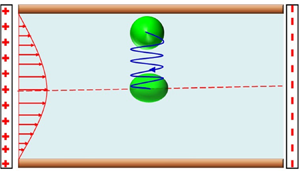
The two-dimensional (2-D) computational domain is shown in figure 1, where a neutrally buoyant leaky dielectric droplet is suspended in another leaky dielectric medium under the combined governance of oscillatory pressure-driven background flow and uniform axial electric field. As the computations are planar (2-D), the undeformed droplet is circular in shape. The computational domain is bounded by the top wall boundary (BT), bottom wall boundary (BB), inlet left-side boundary (BL) and the outlet right-side boundary (BR). The radius of the droplet is denoted by a. The initial location of the droplet from the bottom wall boundary is  $Y_d^\ast $. The electrodes are located at the side boundaries (BL and BR). Thus, an axial electric field, E* acts on the droplet. In this study, a Cartesian coordinate system is adopted, which is fixed at the bottom wall boundary, as depicted in figure 1.
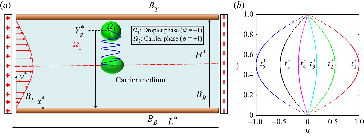
Figure 1. (a) Schematic of the rectangular computational domain. The length and width are L* and H*, respectively. The numerical set-up is bounded by the top and bottom bounding walls (BT, BB) and the left and right boundaries (BL, BR). The initial distance of the droplet from the lower electrode is denoted by the  $Y_d^\ast $. (b) Time sequence of the velocity profile, where $t_6^\ast \gt t_5^\ast \gt t_4^\ast \gt t_3^\ast \gt t_2^\ast \gt t_1^\ast $.
2.1. Numerical simulation: phase field method
For computational modelling of the physical problem described previously, we adapt the phase field method (Jacqmin Reference Jacqmin1999; Badalassi, Ceniceros & Banerjee Reference Badalassi, Ceniceros and Banerjee2003; Mandal et al. Reference Mandal, Ghosh, Bandopadhyay and Chakraborty2015b). In previously reported studies (Wang, Qian & Sheng Reference Wang, Qian and Sheng2008; Mandal et al. Reference Mandal, Ghosh, Bandopadhyay and Chakraborty2015b; Chaudhury et al. Reference Chaudhury, Mandal and Chakraborty2016), several authors mentioned the utility of this method in capturing the interfacial dynamics of a two-fluid system. It is important to mention that the method is premised on the minimization of the total energy of the system and is thermodynamically consistent (Chakraborty Reference Chakraborty2007, Reference Chakraborty2008Reference Chakraborty and Durst). Owing to its flexible generalized framework, it allows the incorporation of appropriate physics by suitably altering the free energy functional. In the phase field method, for identifying the distribution of constituting fluid phases, an order parameter, ψ (x,t) is used. In figure 1, the droplet and surrounding fluid medium are denoted by ψ = −1 and +1, respectively. The values of ψ vary between −1 and 1 in the diffuse interfacial region. The dynamic evolution of ψ is described by the Cahn–Hilliard equation. This equation comprises both the advection as well as diffusion terms and reads (Jacqmin Reference Jacqmin1999; Mandal et al. Reference Mandal, Ghosh, Bandopadhyay and Chakraborty2015b)
 \begin{equation}\frac{{\partial \psi }}{{\partial {t^ \ast }}} + {\boldsymbol{u}^ \ast }{\bf \cdot }{\boldsymbol{\nabla} ^ \ast }\psi = {\boldsymbol{\nabla} ^ \ast }{\bf \cdot }(M_\psi ^\ast {\boldsymbol{\nabla} ^ \ast }{G^\ast }),\end{equation}
where the mobility factor and the chemical potential are denoted by  $M_\psi ^\ast ,{G^\ast }$, respectively. Here G* is described as ${G^\ast } = \gamma ({\psi ^3} - \psi )/{\xi ^\ast } - \gamma {\xi ^\ast }{\boldsymbol{\nabla} ^{\ast 2}}\psi$. The interfacial thickness is denoted by ${\xi ^\ast }$. In this work, asterisks are used to denote dimensional parameters, for notational convenience.
In the framework of phase field formalism, any generic fluid property (χ*) can be suitably interpolated via the distribution of the order parameter (Badalassi et al. Reference Badalassi, Ceniceros and Banerjee2003; Yang, Li & Ding Reference Yang, Li and Ding2013; Mandal et al. Reference Mandal, Ghosh, Bandopadhyay and Chakraborty2015b; Yang et al. Reference Yang, Li, Zhao, Shao and Xu2016):
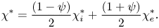 \begin{equation}{\chi ^\ast } = \frac{{(1 - \psi )}}{2}\chi _i^\ast + \frac{{(1 + \psi )}}{2}\chi _e^\ast .\end{equation}
In a non-dimensional format, this is expressed as
 \begin{equation}\chi = \frac{{(1 - \psi )}}{2}{\chi _r} + \frac{{(1 + \psi )}}{2},\quad \textrm{where}\,{\chi _r} = \chi _i^\ast /\chi _e^\ast .\end{equation}
2.2. Governing equations and boundary conditions
2.2.1. Electric field
As the electric field is irrotational  $({\boldsymbol{\nabla} ^\ast } \times {\boldsymbol{E}^\ast } = 0)$, it may be related to the electric potential as ${\boldsymbol{E}^\ast } = - {\boldsymbol{\nabla} ^\ast }\phi $. Forces of electrical origin may be expressed in terms of the divergence of the Maxwell stress tensor, so that
 \begin{equation}{\boldsymbol{F}^{\ast E}} = \int_\forall {({\boldsymbol{\nabla} ^\ast }{\bf \cdot }{\boldsymbol{{T}}^{\ast M}})} \,\textrm{d}{x^{\ast 3}},\quad {\boldsymbol{\nabla} ^\ast }{\bf \cdot }{\boldsymbol{{T}}^{\ast M}} = q_v^\ast {\boldsymbol{E}^\ast } - \frac{1}{2}({\boldsymbol{E}^\ast }{\bf \cdot }{\boldsymbol{E}^\ast }){\bf \cdot }{\boldsymbol{\nabla} ^\ast }\varepsilon ,\end{equation}
where ∀ symbolizes the domain volume, and the Maxwell stress tensor is denoted by  ${\boldsymbol{T}^{\ast M}}$. The first term of (2.4) denotes the Coulomb force (or electric force), which appears because of the interaction between the electric field and free charges. The second term refers to dielectrophoretic force. In (2.4), qv denotes the bulk-free charge density. In accordance with Gauss law, one may write
 \begin{equation}{\boldsymbol{\nabla} ^\ast }{\bf \cdot }(\varepsilon {\boldsymbol{\nabla} ^\ast }\phi ) = q_v^\ast .\end{equation}
Following the generic property interpolation scheme described earlier, ε can be described as
 \begin{equation}\varepsilon = \frac{{(1 - \psi )}}{2}{\varepsilon _i} + \frac{{(1 + \psi )}}{2}{\varepsilon _e}.\end{equation}
Further, from charge conservation consideration, the bulk-free charge density follows the following governing equation:
 \begin{equation}\frac{{\textrm{D}q_v^\ast }}{{\textrm{D}{t^ \ast }}} + {\boldsymbol{\nabla} ^ \ast }{\bf \cdot }(\sigma {\boldsymbol{E}^ \ast }) = \frac{{\partial q_v^\ast }}{{\partial {t^\ast }}} + {\boldsymbol{\nabla} ^ \ast }{\bf \cdot }(q_v^\ast {\boldsymbol{u}^ \ast }) + {\boldsymbol{\nabla} ^ \ast }{\bf \cdot }(\sigma {\boldsymbol{E}^ \ast }) = 0.\end{equation}
In accordance with the leaky-dielectric theory (Taylor Reference Taylor1966; Melcher & Taylor Reference Melcher and Taylor1969), free charges are transferred instantly from bulk fluid to the interfacial region and the bulk fluid becomes free of charge. Hence,  $\textrm{D}q_v^\ast /\textrm{D}{t^\ast } = 0$ and (2.7) is reduced to the following form:
 \begin{equation}{\boldsymbol{\nabla} ^\ast }{\bf \cdot }(\sigma {\boldsymbol{E}^\ast }) = 0.\end{equation}
Using the irrotationality of the electric field, (2.8) can be expressed as
 \begin{equation}{\boldsymbol{\nabla} ^\ast }{\bf \cdot }(\sigma {\boldsymbol{\nabla} ^\ast }\phi ) = 0.\end{equation}
Here  $\sigma $ is interpolated as $\sigma = ((1 - \psi )/2){\sigma _i} + ((1 + \psi )/2){\sigma _e}$.
At the inlet and outlet boundaries, the electric potential follows the boundary conditions as stated in the following:
 \begin{equation}\left. \begin{array}{l} \textrm{At}\,\textrm{inlet}\,\textrm{boundary}\,({B_L}):{\phi^\ast } = 0\,\textrm{at}\,{x^\ast } = 0,\\ \textrm{At}\,\textrm{outlet}\,\textrm{boundary}\,({B_R}):{\phi^\ast } = {L^\ast }E_\infty^\ast \,\textrm{at}\,{x^\ast } = {L^\ast }. \end{array} \right\}\end{equation}
2.2.2. Fluid flow
The governing continuity and momentum equations for fluid flow are given by
 \begin{gather}{\boldsymbol{\nabla} ^\ast }{\bf \cdot }{\boldsymbol{u}^\ast } = 0,\end{gather}
 \begin{gather}\begin{array}{ccccc} \rho \left( {\dfrac{{\partial {\boldsymbol{u}^\ast }}}{{\partial {t^\ast }}} + {\boldsymbol{\nabla}^\ast }{\bf \cdot }({\boldsymbol{u}^\ast }{\boldsymbol{u}^\ast })} \right) & = - {\boldsymbol{\nabla} ^\ast }{p^\ast } + {\boldsymbol{\nabla} ^\ast }{\bf \cdot }[\mu \{ {\boldsymbol{\nabla} ^\ast }{\boldsymbol{u}^\ast } + {({\boldsymbol{\nabla} ^\ast }{\boldsymbol{u}^\ast })^\textrm{T}}\} ]\\ & \quad +\, {G^\ast }{\boldsymbol{\nabla} ^\ast }\psi + {\boldsymbol{F}^{\ast E}} + F_o^\ast {\bf }\sin ({\omega ^\ast }{t^\ast }){{\boldsymbol{\mathord{\buildrel{\lower3pt\hbox{$\scriptscriptstyle\frown$}} \over e} }}_x}. \end{array}\end{gather}
 Equation (2.12) couples the electrohydrodynamics with phase field formalism, where  ${G^\ast }{\boldsymbol{\nabla} ^\ast }\psi $ acts as a representation of the interfacial tension in terms of the phase field order parameter and the chemical potential and ${\boldsymbol{F}^{\ast E}}$ denotes the electric body force as stated in (2.4). Here $F_o^\ast \sin ({\omega ^\ast }{t^\ast })$ represents the oscillatory component of the driving pressure gradient, where ω* and $F_o^\ast $ represent the frequency and amplitude of the imposed oscillation, respectively.
2.3. Normalization of governing equations
Normalized forms of the governing equations, described previously, read
 \begin{gather}\frac{{\partial \psi }}{{\partial \bar{t}}} + \boldsymbol{u}{\bf \cdot\boldsymbol{\nabla} }\psi = \frac{1}{{Pe}}{\boldsymbol{\nabla} ^2}G,\quad \textrm{where}\,G = \frac{1}{{Cn}}({\psi ^3} - \psi ) - Cn{\boldsymbol{\nabla} ^2}\psi ,\end{gather}
 \begin{gather}\boldsymbol{\nabla}\boldsymbol{\cdot}(\sigma \boldsymbol{\nabla}\phi ) = 0,\end{gather}
 \begin{gather}{\bf \boldsymbol{\nabla} \cdot}\boldsymbol{u} = 0,\end{gather}
 \begin{gather}Re\left(\frac{{\partial \boldsymbol{u}}}{{\partial t}} + \boldsymbol{u}\boldsymbol{\cdot}\boldsymbol{\nabla} \boldsymbol{u}\right) = - \boldsymbol{\nabla}p + \boldsymbol{\nabla}\boldsymbol{\cdot}[\mu \{ \boldsymbol{\nabla}\boldsymbol{u} + {(\boldsymbol{\nabla}\boldsymbol{u})^\textrm{T}}\} ] \nonumber \\ + \frac{1}{{Ca}}\boldsymbol{\cdot }G\boldsymbol{\nabla} \psi\, {+}\, \frac{{C{a_E}}}{{Ca}}{\boldsymbol{F}^E} + 8\sin (t\,St){\boldsymbol{\mathord{\buildrel{\lower3pt\hbox{$\scriptscriptstyle\frown$}} \over e} }_x}.\end{gather}
For the normalization scheme, the following scaling parameters are used: length scale H*, velocity scale u*c, time scale  ${H^\ast }/u_c^\ast $, viscous stress scale ${\mu _e}u_c^\ast /{H^\ast }$, electric field scale $E_\infty ^\ast $ and electric stress scale ${\varepsilon _e}E_\infty ^{\ast 2}$. Here H* and u* denote the channel height and centreline flow velocity, respectively. The consequent normalization results in the following dimensionless parameters: Reynolds number $(Re = \rho u_c^\ast {H^\ast }/{\mu _e})$, Péclet number $(Pe = {H^{\ast 2}}{u_c}/M_\psi ^\ast \gamma )$, capillary number $(Ca = \mu u_c^\ast /\gamma )$, electric capillary number $(C{a_E} = {\varepsilon _e}E_\infty ^{\ast 2}{H^\ast }/\gamma )$, Cahn number $(Cn = {\xi ^\ast }/{H^\ast })$ and Strouhal number $(St = {\omega ^\ast }{H^\ast }/u_c^\ast )$. Another important dimensionless parameter is the confinement ratio (Wc), defined as the ratio of undeformed droplet diameter to the width of the channel (expressed as Wc = 2a*/H*). In the present analysis, we consider L (= L*/H*) = 3.
Interpolation of physical properties, in a dimensionless form, reads (Mondal et al. Reference Mondal, Ghosh, Bandopadhyay, DasGupta and Chakraborty2014)
 \begin{equation}\left. {\begin{aligned} {\rho = \dfrac{{(1 - \psi )}}{2}{\rho_r} + \dfrac{{(1 + \psi )}}{2};\,{\rho_r} = \dfrac{{{\rho_i}}}{{{\rho_e}}}}\\ {\mu = \dfrac{{(1 - \psi )}}{2}\lambda + \dfrac{{(1 + \psi )}}{2};\,\lambda = \dfrac{{{\mu_i}}}{{{\mu_e}}}}\\ {\varepsilon = \dfrac{{(1 - \psi )}}{2}S + \dfrac{{(1 + \psi )}}{2};\,S = \dfrac{{{\varepsilon_i}}}{{{\varepsilon_e}}}}\\ {\sigma = \dfrac{{(1 - \psi )}}{2}R + \dfrac{{(1 + \psi )}}{2};\,R = \dfrac{{{\sigma_i}}}{{{\sigma_e}}}} \end{aligned}} \right\},\end{equation}
As the interacting fluids are neutrally buoyant for the case studies addressed in this work, we have set ρ = ρr = 1 subsequently.
The boundary conditions employed at the top and bottom walls (BT and BB) in dimensionless forms read
 \begin{equation}\left. \begin{array}{* {20}{c@{}}} {\textrm{(i)}\,\textrm{No}\,\textrm{slip}:\,\boldsymbol{u} - (\boldsymbol{u}\,\boldsymbol{\cdot}{\boldsymbol{n}_s}){\boldsymbol{n}_s} = \mathbf{0},}\\ {\textrm{(ii)}\,\textrm{No}\,\textrm{penetration:}\,\boldsymbol{u}\boldsymbol{\cdot}{\boldsymbol{n}_s} = 0,}\\ \textrm{(iii)}\,\textrm{No}\,\textrm{flux}:\,{\boldsymbol{n}_s}\,\boldsymbol{\cdot}\, \boldsymbol{\nabla} \psi = 0. \end{array} \right\}\end{equation}
Here,  ${\boldsymbol{n}_s}$ denotes the normal vector at the walls. The governing equations have been solved using the finite element method taking the mentioned boundary conditions into consideration (Mandal et al. Reference Mandal, Ghosh, Bandopadhyay and Chakraborty2015b; Santra et al. Reference Santra, Sen, Das and Chakraborty2019b; Wang et al. Reference Wang, Jones, Gralnick, Lin and Buie2019). The details of the numerical implementation are described in the supplementary material available at https://doi.org/10.1017/jfm.2020.789.
3. Results and discussion
3.1. Model benchmarking
In an effort to benchmark our numerical model, we have first conducted validation studies vis-à-vis the results reported by Halim & Esmaeeli (Reference Halim and Esmaeeli2013), Mortazavi & Tryggvason (Reference Mortazavi and Tryggvason2000), Chaudhury et al. (Reference Chaudhury, Mandal and Chakraborty2016) and Ha & Yang (Reference Ha and Yang2000). Ha & Yang (Reference Ha and Yang2000) experimentally investigated the electric-field-induced deformation and breakup characteristics of Newtonian and non-Newtonian droplets.
For comparison, we have chosen system NN21 from their study, where castor oil and silicone oil (μ* = 0.90 Pa⋅s) have been used as the droplet phase and suspending fluid phase, respectively. In the sole presence of an electric field, the droplet either deforms into prolate or oblate configuration depending on the relative electrical properties. The degree of the deformation of the droplet is measured by the deformation parameter, D (Taylor Reference Taylor1966), expressed as D = (Lmax − Lmin)/(Lmax + Lmin), where Lmax and Lmin are the length of the major axis and minor axis of the elliptically deformed (prolate or oblate) droplet, respectively. In the study reported by Halim & Esmaeeli (Reference Halim and Esmaeeli2013), they have employed the front-tracking/finite difference method to study the transient electrohydrodynamic behaviour of leaky dielectric droplet under uniform electric field. In the numerical study performed by Chaudhury et al. (Reference Chaudhury, Mandal and Chakraborty2016), they have analysed the migration characteristic of the droplet in the presence of background oscillatory flow field in a parallel plate microchannel. Mortazavi & Tryggvason (Reference Mortazavi and Tryggvason2000) have performed a numerical study on the cross-stream motion of the deformable droplet in pressure-driven flow, taking the effect of finite inertia, the viscosity ratio of the fluids and the interfacial tension into consideration. In this study, they have used a front-tracking/finite difference method to numerically simulate the problem. Figure 2(a) depicts an excellent agreement between the findings of Halim & Esmaeeli (Reference Halim and Esmaeeli2013) and predictions based on the present numerical set-up, highlighting the temporal variation of the electric field-induced deformation of droplet for different values of the permittivity ratio. Figure 2(b) also presents another comparison of the cross-stream motion of the droplet between the present findings and the numerical results of Mortazavi & Tryggvason (Reference Mortazavi and Tryggvason2000), exhibiting excellent quantitative agreement. In addition, figure 2(c) illustrates a comparison between the present numerical results and experimental results of Ha & Yang (Reference Ha and Yang2000) on the electric-field-induced alteration of the steady-state deformation of the droplet, illustrating favourable agreement. Figure 2(d) depicts a comparison between our numerical results and the results of Chaudhury et al. (Reference Chaudhury, Mandal and Chakraborty2016) on the cross-stream migration of the droplet under an oscillatory flow field. Excellent agreement is also obtained in this regard. All these benchmarking studies also involve a rigorous grid independence (equivalently, Cahn number independence) study and Péclet number independence test, which have not been detailed in this work for the sake of brevity. These validations enable benchmarking optimal grid sizing in the computational domain, based on the consideration of Cahn number independence (equivalently, grid independence). The details of the Cahn number independence and grid independence studies are given in the supplementary material.
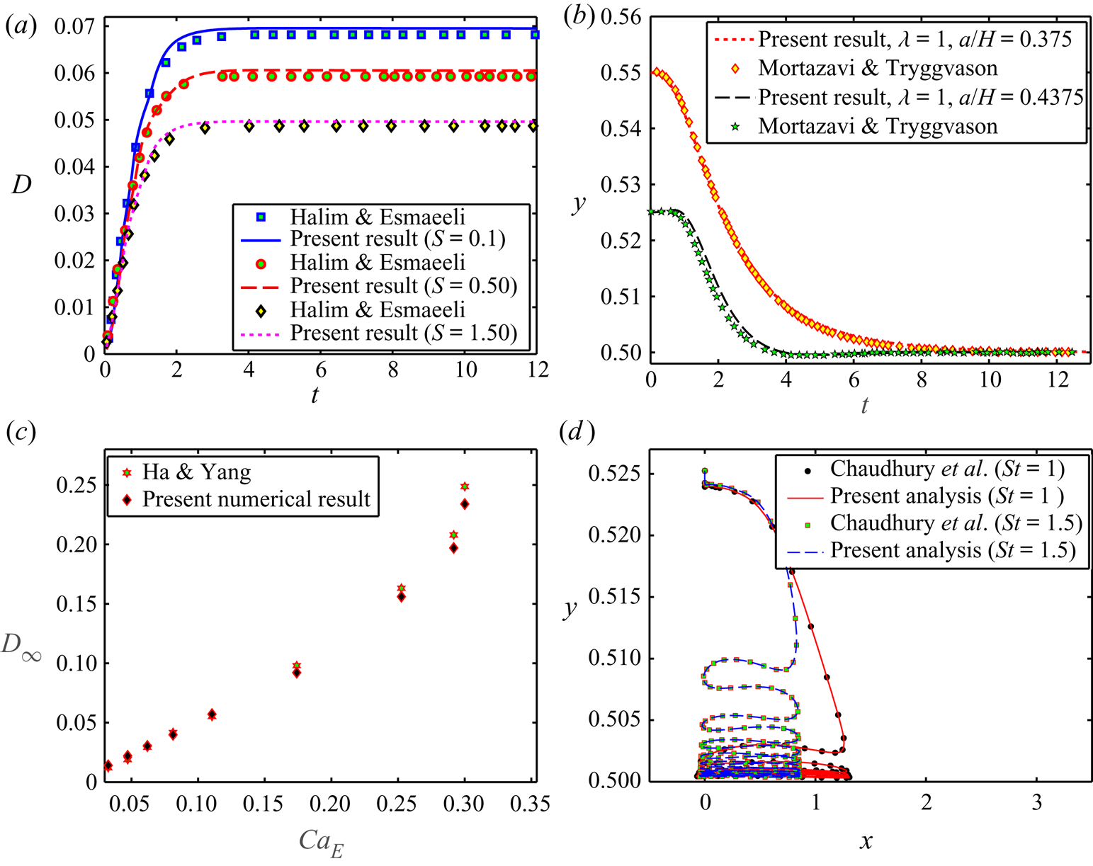
Figure 2. (a) Temporal variation of the deformation parameter in the presence of a uniform electric field, considering the set-up of Halim & Esmaeeli (Reference Halim and Esmaeeli2013). Important parameters are R = 2.5, λ = 0.1, CaE = 0.25 and Re = 1. (b) Temporal variation of the transverse position of the droplet's centroid, considering the set-up of Mortazavi & Tryggvason (Reference Mortazavi and Tryggvason2000). Important parameters are ρr = 1, Re = 1 and Ca = 0.33. (c) Variation of steady-state parameters (D∞) with electric field strength (CaE), considering the set-up of Ha & Yang (Reference Ha and Yang2000). Important parameters are (R, S) = (10, 1.37), Re = 0.01 and λ = 0.874. (d) Cross-stream migration characteristics of the droplet in the presence of oscillatory pressure gradient-driven flow in parallel plate micro-confinement, considering the set-up of Chaudhury et al (Reference Chaudhury, Mandal and Chakraborty2016). Important parameters are a = 0.4375, Ca = 0.286, ρr = 1, λ = 1, Re = 1.
3.2. Alteration in droplet motion in the combined presence of an electric field and background oscillatory flow
3.2.1. Electric-field-induced modification in cross-stream motion of the droplet
Figure 3 depicts the influence of a steady axial electric field on the cross-stream motion of the droplet for a model system based on the problem description outlined schematically in figure 1. Values of the relevant dimensionless parameters (unless they are varied) used for generating these results are (S, R) = (2, 0.5), ρr = 1 and λ = 1. These collective properties conform to a specific category of physical system designated as system A. In the present analysis, depending on the relative strength of electric stress as compared with the flow-induced viscous stress, we have classified the magnitude of electric field strength into three categories: (i) low electric field strength (where CaE ≤ 0.5 and Ca = 0.3); (ii) moderate electric field strength (0.5 < CaE ≤ 1.5 and Ca = 0.3); (iii) high electric field strength (CaE > 1.5 and Ca = 0.3).

Figure 3. (a) Cross-stream migration characteristic of the droplet in oscillatory microflow, (b) Temporal variation of the transverse position of the droplet's centroid. The variation of tss with CaE is shown in the inset of figure 3(b). Important simulation parameters are (S, R) = (2, 0.5), Ca = 0.3, Yd = 0.525, ρr = 1, λ = 1, a = 0.3, Re = 0.1 and St = 2.
The shape evolution of the droplet at different stages of the cycle of the imposed oscillation is also shown in figure 3. In the sole presence of oscillatory pressure-driven flow, the droplet moves towards the centreline in a zig-zag pathway without any net axial displacement (defined as oscillatory motion). However, when an axial electric field is applied, figure 3(a) clearly depicts that the axial oscillations of the droplet prior to reaching the domain centreline dampen out, and the droplet follows an uncurling pathway (defined as non-oscillatory motion) at high values of CaE. Once the droplet arrives at the centreline, it continues to oscillate in the axial direction. Figure 3(b) further emphasizes that the time taken by the droplet to achieve its steady-state transverse position (tss) also decreases with the rise in the relative strength of the electric field. Though this phenomenon appears intuitive, it is of fundamental importance in the exploration of several practical problems of outstanding relevance, such as high-throughput and on-demand sorting of deformable entities (droplet, biological cells, etc.) in confined micro-environments. In this regard, it should be mentioned that despite a widespread emergence of oscillatory microfluidics towards sorting soft fluidic and cellular matters under physiologically relevant conditions, one important inherent limitation of the same has been reported to be the fact that the sorting process takes place very sluggishly, bearing adverse consequences on the net throughput. The findings of figure 3 illustrate that the presence of the axial electric field offers a remedy to overcome this constraint to a large and controllable extent.
Similarly, figure 4 illustrates the electric-field-induced modification of the cross-stream migration of the droplet for another physical system, henceforth termed as system B. The distinctive hallmark of system B, as compared with system A, is as follows: the conductivity ratio (R) of the system is higher than the permittivity ratio (S) that essentially creates the electrohydrodynamic flow from poles to equators. Relevant dimensionless properties are (S, R) = (0.5, 2), ρr = 1 and λ = 1. From figure 4(a), it is evident that the axial oscillations of the droplet before reaching the centreline are amplified for moderate values of CaE (= 1 and 1.5). Hence, the value of tss increases as depicted in figure 4(b). If we slightly increase the value of CaE (= 1.52), the droplet achieves its steady-state transverse position almost immediately (tss = 0.583). In this case, the ultimate position of the droplet (= 0.5252) is nearly equal to its initial position (= 0.525). For this value of CaE, the axial oscillation of the droplet before reaching steady-state transverse position disappears completely. However, after reaching the steady-state transverse position, the droplet undergoes axial oscillations along a horizontally straight pathway. If we further increase the value of CaE (= 2), the steady-state transverse position of the droplet shifts towards the upper wall and the axial oscillations of the droplet before reaching the final position again amplifies. Accordingly, the magnitude of tss increases. However, if we raise the value of CaE beyond a threshold limit (CaE = 5), not only do the axial oscillations attenuate, but the droplet also moves towards the nearest wall at a faster rate. Hence the magnitude of tss, again, reduces. Therefore, for this leaky dielectric system, the magnitude of tss varies non-monotonically with the values of CaE. This phenomenon has immense importance in efficient and rapid manipulation of biological and non-biological deformable entities at will in a microfluidic system, constrained by its axial length.

Figure 4. (a) Cross-stream migration characteristic of the droplet in an oscillatory microflow, (b) Temporal variation of the transverse position of the droplet's centroid. The variation of tss with CaE is shown in the inset of figure 4(b). Important simulation parameters are (S, R) = (0.5, 2), Ca = 0.3, Yd = 0.525, ρr = 1, λ = 1, a = 0.3, Re = 0.1 and St = 2.
We now discuss the physical reasoning behind these observations. In a steady pressure-driven flow, the droplet's cross-stream motion in microchannel occurs owing to (i) hydrodynamic force (FH), originating out of the streamline curvature and deformed shape of the droplet, and (ii) non-inertial lift force (FL), stemming from the wall effects. However, when the droplet is subjected to oscillatory pressure-driven flow, FH becomes oscillating in nature and creates oscillations in the droplet that hinders the droplet's motion in the transverse direction. The imposed oscillation is quantitatively characterized by the dimensionless oscillation frequency or the Strouhal number, St. For high values of St, the imposed oscillation arrests the transverse motion of the droplet to a considerable extent. However, in the presence of an electric field, two additional forces also act on the droplet and modify droplet's migration characteristics in a dramatic fashion. These forces are (i) dielectrophoretic force  $({F_D} = - 1/2 \cdot {E^2} \cdot \boldsymbol{\nabla}\varepsilon )$ and (ii) electrohydrodynamic force (FEHD).
Although variations in electrical permittivity trigger dielectrophoretic forces, the asymmetric distribution of electric shear-driven flow circulation generates electrohydrodynamic forces. The net dielectrophoretic force always attempts to drive the droplet towards the wall in closer vicinity, irrespective of the electrical properties of the system. This phenomenon can be justified through figure 5(a), where the variation of E 2 is plotted along a vertical line, drawn from the bottom wall to top wall and going through the centroid of the droplet.
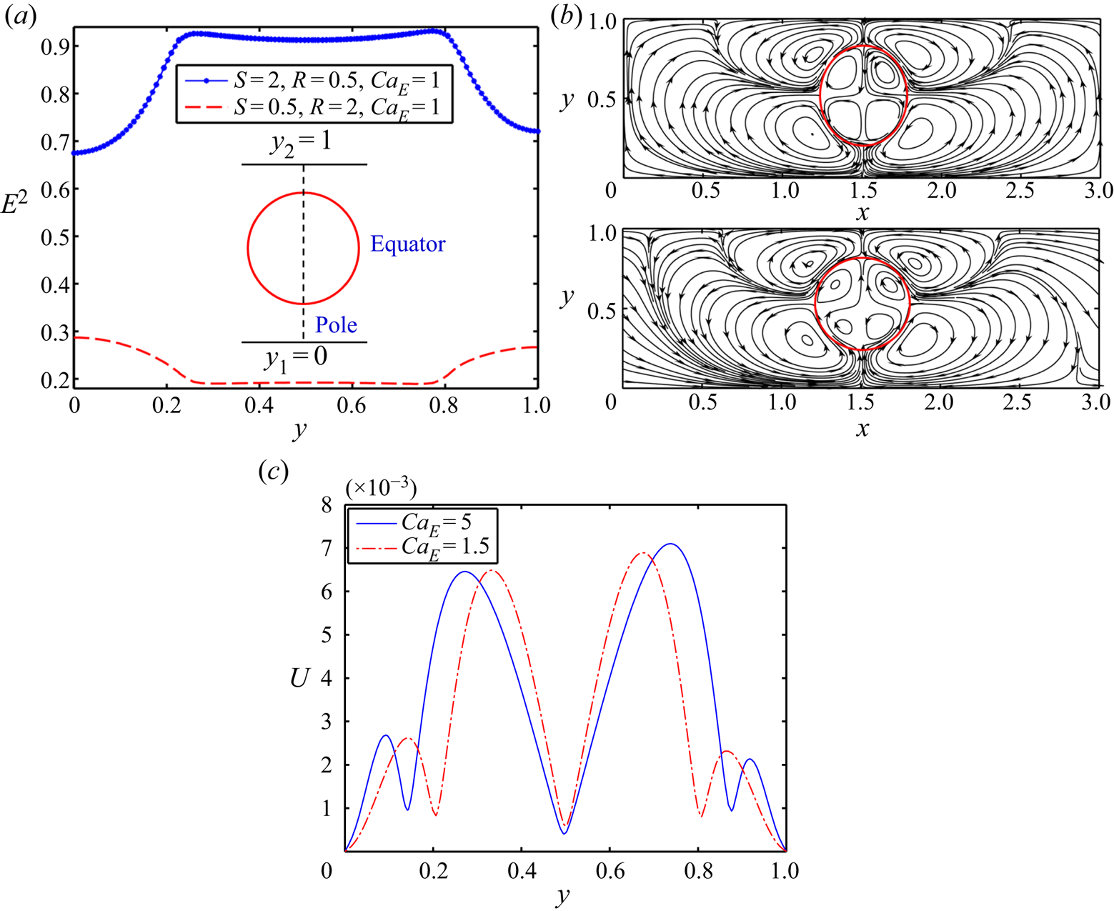
Figure 5. The influence of electric field on the droplet. (a) Variation of E 2 along a vertical straight line passing from lower wall to the upper wall through the centroid of the droplet. Streamline pattern of flow circulation, formed in the presence of an electric field for (b) system A having (S, R) = (2, 0.5) and (c) system B having (S, R) = (0.5, 2). For (a–c), the value of CaE is 1.5. (d) Variation of the magnitude of velocity along a probe passing through the centroid of the droplet and drawn from the lower wall to the upper wall for system A having (R, S) = (0.5, 2). Other parameters are Yd = 0.525, ρr = 1, λ = 1, a = 0.3, t = 2.5 and Re = 0.1.
Figure 5(a) illustrates that, for system A, the strength of E 2 is higher at the bottom side of the droplet as compared with its top side. Again, the magnitude of the E 2 is lower in the ambient fluid with respect to the inside fluid of the droplet. Similarly, for system B, the strength of E 2 is higher and lower at the bottom half and the top half of the droplet, respectively, and the strength of E 2 is higher outside the droplet with respect to its inner region. This symmetry breaking in E 2 creates an imbalance in dielectrophoretic force at the two surfaces, producing a translational motion of the droplet in the upward direction (Esmaeeli Reference Esmaeeli2016). However, the net FEHD can drive the droplet toward the wall or channel centreline based on the direction of electric-shear-driven flow circulation around the droplet which is further determined from the conductivity ratio (R) and permittivity ratio (S). Under a steady axial electric field, for system A, the direction of the flow circulation is from the equator to the poles as depicted in figure 5(b). Thus, for system A, the net FEHD tries to drive the droplet toward the centreline. Briefly, in system A, when a droplet is placed above the centreline, the electric field creates two asymmetric vortex pairs inside the droplet as depicted in figure 5(b). Therefore, the FEHD, arising because of the inner vortex at the top half and bottom half (with respect to the horizontal line of symmetry) of the droplet, attempts to drive the droplet toward the centreline and nearby wall, respectively. Figure 5(d) shows that the magnitude of the velocity is greater inside the droplet in the upper half. Hence, the strength of the generated FEHD owing to inner vortex pairs at the upper half is significantly higher with respect to that in the lower half.
Owing to this fact, the net FEHD due to the dynamics of the inner vortex attempts to set the droplet in motion towards the channel centreline. Similar to the inner vortex pair, counter-rotating pairs of outer vortices are generated just outside the droplet. The FEHD owing to outer vortex pairs at the top side or bottom side attempts to pull the droplet towards the nearest wall and the channel centreline, respectively. From figure 5(d), we observe that the strength of the outer vortex pair at the bottom half of the droplet is greater than the top half. Hence, the net FEHD caused by the dynamics of the outer vortex also pulls the droplet towards the channel centreline. One can infer that the resultant effect of the net FEHD due to the dynamics of vortices drives the droplet towards the centreline. It is worth mentioning that the strength of the net FEHD depends on the strength of the flow circulation, which again relies on the strength of the electric field. Figure 5(d) shows that for system A, with the enhancement of CaE, the strength of the flow circulations in the inner vortex at the top half and outer vortex at the bottom half increases, which amplifies the strength of the net FEHD. Thus, for system A, the direction and the patterns of the droplet motion are determined by the interplay among FH, FL, FD and FEHD. For system A, at higher values of CaE, the strength of the net FEHD increases drastically and becomes dominant over the other forces that drive the droplet to the centreline at a faster rate in an unwinding pathway.
Similar to system A, in system B the interplay among the FH, FL, net FD and net FEHD also dictates the direction and pattern of the cross-stream motion of the droplet. However, for system B, the direction of electrohydrodynamic flow takes place from poles to the equators as depicted in figure 5(c). Therefore, the net FEHD tries to drive the droplet towards the nearby wall. In short, in system B, when a droplet is kept above the centreline, the electric field creates two asymmetric vortex pairs inside the droplet, as illustrated in figure 5(c). Hence, FEHD, arising because of the inner vortex at the top half and the bottom half (with respect to the horizontal line of symmetry) of the droplet, attempts to move the droplet toward the adjacent wall and centreline, respectively. Along with inner vortex pairs, two pairs of counter-rotating outer vortices are also formed. The FEHD originating out of the outer vortex pairs at the upper half of the droplet tries to push the droplet towards the centreline, whereas the FEHD owing to the outer vortex pair at the bottom half of the droplet tries to push the droplet towards the nearby wall.
Figure 6(a) shows that the strength of inner vortex pairs and the outer vortex pairs is high at the upper half and lower half of the droplet, respectively. Therefore, the net FEHD owing to the dynamics of the vortex pairs attempts to move the droplet towards the nearby wall. Furthermore, as we mentioned earlier, the net FD arising owing to the asymmetric distribution of E 2 also attempts to push the droplet towards the nearby wall. On the other hand, the forces FL and FH attempt to move the droplet towards centreline, opposing these effects. At a moderate value of CaE (= 1.5), figure 6(a) shows that the strength of the flow circulation is comparatively weak. Therefore, the strength of net FEHD is also relatively low. Similarly, figure 6(b) also confirms that the magnitude of E 2 is also comparatively lower for CaE = 1.5. Hence, for this value of CaE, the united strength of net FEHD and FD is also not significantly high. Therefore, in this scenario, the combined effect of FH and FL remains dominating in nature. Owing to the opposing nature of net FEHD and FD, they attempt to lessen the combined effect of FH and FL. As a result, for CaE = 1.5, the transverse component droplet's velocity (udy) towards the centreline reduces, as depicted in figure 7. Because the magnitude of udy is low for CaE = 1.5 and the considered value of the St is considerably high (St = 2), the droplet takes greater time to reach the centreline and exhibits more number of oscillations before arriving at the centreline. Therefore, the magnitude of tss also increases. If we further increase the value of CaE, the magnitude of net FEHD and FD also increases. At CaE = 1.52, the united effect of net FEHD and FD nullifies the combined strength of FH and FL almost instantaneously, and the droplet immediately attains a steady-state position. Therefore, the magnitude of tss also reduces drastically. For further increase in the value of CaE (= 2), the integrated strength of net FEHD and FD becomes dominant in nature and shifts the steady-state transverse position towards the upper wall. In this scenario, the axial oscillations of the droplet before reaching the steady-state position again amplify and the magnitude of tss also increases. However, on further increase of CaE (= 5), the magnitude of strength of flow circulation and the magnitude of E 2 enhance significantly, as shown in figures 6(a) and 6(b), respectively. Therefore, the integrated strength of net FEHD and FD enhances markedly. This not only arrests axial oscillations in the cross-stream motion, but also increases the magnitude of udy drastically (as shown in figure 7), which leads to the faster rate of droplet motion toward the wall closest to it.

Figure 6. (a) Variation of the magnitude of velocity along a probe passing through the centroid of the droplet and drawn from the lower wall to the upper wall for system B. (b) Variation of E 2 along a vertical straight line passing from the lower wall to the upper wall through the centroid of the droplet for system B. Other parameters are Yd = 0.525, (R, S) = (2, 0.5), a = 0.3, t = 2.5, Re = 0.1 and λ = 1.
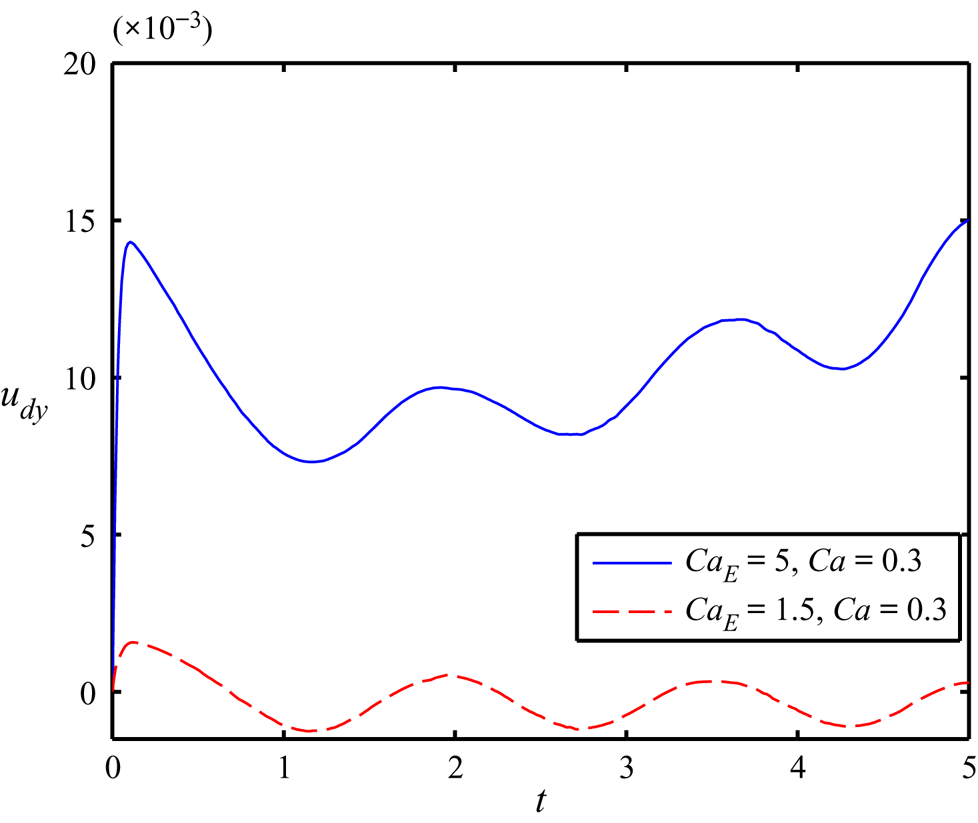
Figure 7. Effect of the electric capillary number on udy (y-component of the velocity of the droplet) in the combined presence of a steady axial electric field and background oscillatory flow. Others parameter are (S, R) = (0.5, 2), Yd = 0.525, a = 0.3, λ = 1 and Re = 0.1.
A critical assessment of the intricate interplay of electromechanical and hydrodynamic forces described previously reveals that the combined effect of the steady axial electric field and the oscillatory pressure-gradient-driven flow on the droplet's drift velocity is not necessarily a mere linear superposition of the droplet's velocity obtained in an oscillatory flow and steady axial electric field, separately. This is due to the two-way nonlinear coupling between electric potential and flow field mediated by unique shape modulation: the applied electric field modifies the fluid flow by developing Maxwell stress at the interface of the droplet; dynamical evolution of the droplet's shape being unknown a priori. Again, this flow field causes the deformation of the droplet, which, in turn, modifies the electric potential distribution. Owing to the fact that the intrinsic cause of the coupled nature of the electromechanics and hydrodynamics is the shape deformation of the droplet, the resultant effect of oscillatory flow and electric field can be combined by simply adding together the respective drift velocities only in small deformation limits. Although this represents the essential qualitative physics, a more quantitative depiction is presented in the following.
In an effort to offer a quantitative perspective of the conceptual foundation delineated previously, we next depict a regime plot across the Ca−CaE parameter space, in figure 8, to probe the extent of validity of linear superposition of the drift velocities obtained by considering the individual forcing parameters separately. The linear superposition approach is considered to validate the outcome from the combined effect when the difference between them is less than 0.5%. The regime plot clearly shows two distinct regimes: regime 1, comprising ‘rectangular data points’ where the linear superposition is valid; and regime 2, comprising ‘circular data points’, where it fails. Evidently, for low values of Ca (typically, less than 0.01), the linear superposition works up to a comparatively high value of CaE (= 0.06). This may be attributed to the fact that for such low values of Ca, the viscous stress-induced droplet deformation is much less. As the magnitude of Ca increases, this upper limit of CaE (for the validity of the linear superposition) progressively reduces, stemming from a nonlinear interplay between the electromechanics and hydrodynamics as mediated by the droplet deformation. Beyond Ca = 0.06, the viscous stress-induced deformation of the droplet becomes so large that the linear superposition deems completely invalid for any finite, non-zero values of CaE.

Figure 8. Regime plot showing two distinct regimes based on the values of Ca and CaE. Regime 1: the effects of oscillatory flow and axial electric field may be combined by linear superposition of the respective drift velocities. Regime 2: the linear superposition fails. Others parameter are (S, R) = (0.5, 2), Yd = 0.525, a = 0.3, λ = 1 and Re = 0.1.
Next, we construct a regime diagram across the CaE–St parameter space for system A, as shown in figure 9, in an effort to unveil of coupling between the imposed flow oscillation and electrical forcing. In the figure, region A containing blue-coloured circular markers denotes oscillatory downward motion of the droplet, whereas the red-coloured diamond-shaped markers in region B represent oscillation-free downward motion of the same.

Figure 9. Regime plot based on the values of (CaE, St). Other parameters are (S, R) = (2,0.5) Ca = 0.3, a = 0.3, Re = 0.1, λ = 1 and Yd = 0.525.
Figure 9 further suggests that, at low values of the St, the transition of the droplet motion from oscillatory to non-oscillatory state takes place at comparatively low values of CaE. However, on increasing the value of St, the magnitude of CaE necessary for converting the droplet's motion from oscillatory to oscillation-free nature increases. For substantially high values of St, the droplet undergoes oscillatory downward motion for any possible values of CaE. Competing influence of the electric-field-induced net FEHD and the imposed oscillation induced net FH is responsible for such phenomena.
3.2.2. Effect of domain confinement on the cross-stream motion of the droplet
Figure 10 shows the effect of domain confinement on the cross-stream motion of the droplet under the combined influence of steady axial electric field and the background oscillatory flow. The degree of confinement is denoted by the domain confinement ratio (Wc = 2a*/H*). In the present study, we have altered the magnitude of Wc by varying the radius of the droplet keeping other parameters intact. Hence, the effect of the size of the droplet is taken care of by the domain confinement ratio. One primary contribution of the domain confinement manifests via alterations in the hydrodynamic interactions. This alters the balance of the pertinent forces via electrohydrodynamic coupling, triggering transients and cross-stream migration of droplets over small scales, unlike the unbounded scenario (where a ≪ H or Wc ≪ 1)).

Figure 10. Effect of domain confinement on (a) the migration characteristic of the droplet and (b) the temporal variation of the transverse position of the droplet's centroid. The variation of tss with Wc is shown in the inset of (b). Other parameters are (S, R) = (2,0.5), Ca = 0.3, CaE = 1.5, a = 0.3, Re = 0.1, λ = 1, Yd = 0.525 and St = 2.
In addition, figure 10(a) shows that the droplet undergoes oscillatory cross-stream motion following a zig–zag pathway in a weakly confined domain. However, in a tightly confined domain, the axial oscillations before reaching the centreline attenuate. Beyond a threshold value of Wc, the droplet moves to the channel centreline in an uncurling pathway without making axial oscillations. Again, figure 10(b) illustrates that the magnitude of tss also reduces with enhancement of the domain confinement ratio, which dictates more rapid settling of the droplet to its final steady state in highly confined domains.
We now explain the physics behind the observed phenomena described previously. For the considered values of electrical properties, the electrohydrodynamic flow circulation is directed from the equator to poles, as shown in figures 11(a) and 11(b). Hence, the electrohydrodynamic force owing to inner vortex pair at the upper half and outer vortex pairs at the lower half of the droplet attempts to shift the droplet towards the channel centreline. On the other hand, the electrohydrodynamic force owing to the inner vortex pair at the lower half and outer vortex pair at the upper half attempts to push the droplet towards the domain wall. Figure 11(c) depicts that the magnitude of the velocity of the inner vortex is higher at the upper half, as compared with the the lower half, and the difference in the magnitudes of velocity enhances with the increase in relative domain confinement. The consequent increase in the net FEHD attempts to drive the droplet towards the centreline. In a similar way, the net FEHD attributable to the outer vortex also increases with the enhancement of relative domain confinement. Furthermore, with an increase in the relative domain confinement, the strength of FL also enhances. This effect is compounded by enhanced FH in more tightly confined domains. An elevated combined strength of net FEHD, FL and FH, thus, becomes capable of moving the droplet rapidly in an uncurling pathway, with enhancements in the relative domain confinement.
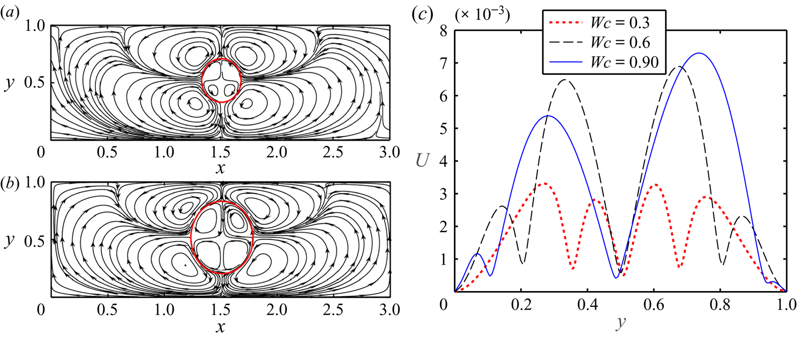
Figure 11. Streamline pattern of flow circulation, formed in the presence an electric field for (a) Wc = 0.3 and (b) Wc = 0.6. (c) Distribution of the magnitude of velocity along a straight line passing through the centreline and drawn from the lower wall to the upper wall. Other parameters are (S, R) = (2,0.5), Ca = 0.3, CaE = 1.5, a = 0.3, Re = 0.1, λ = 1, t = 2.5, Yd = 0.525 and St = 2.
3.2.3. Effect of electrical properties of the system on the cross-stream motion of the droplet
The alteration of the cross-stream motion of the droplet for different values of (R/S) is plotted in figure 12. Figure 12(a) reveals that, with increments in R/S ratio, the axial oscillation of the droplet enhances before reaching the centreline and the transverse extent traversed by the droplet is small. On decreasing the value of R/S, we observe a reduction in the axial oscillations of the droplet, and the transverse distance travelled by the droplet also increases. For comparatively lower values of R/S, the droplet moves to the centreline without undergoing axial oscillations. Figure 12(b) further corroborates that the magnitude of tss decays with the lowering of R/S.
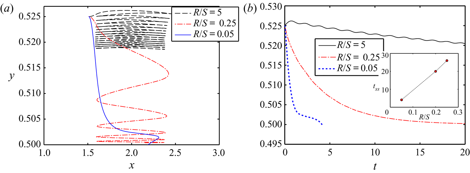
Figure 12. Effect of the electrical property ratio on (a) the cross-stream migration of the droplet and (b) the temporal variation of the transverse position of the droplet's centroid. The variation of tss with R/S is shown in the inset of (b). Other parameters are R = 0.5, Ca = 0.3, CaE = 1.5, a = 0.3, Re = 0.1, λ = 1, Yd = 0.525 and St = 2.
The exclusive dependence of the transverse migration characteristics of the droplet on the relative electrical properties can be explained as follows. In the confined domain, the forces FL and FH attempt to move the droplet towards the domain centreline. On the other hand, for R/S > 1, the direction of electrohydrodynamic flow takes place from the poles to the equator, and the net FEHD owing to the inner vortex pairs at the upper half and outer vortex pair at the lower half of the droplet tries to drive the droplet towards the wall nearest to it. Similarly, the net FD also tries to shift the droplet in a similar direction. The combined consequences of FD and FEHD neutralize the combinatorial effect of FL and FH to a large extent, which leads to amplified axial oscillations of the droplet and decrease in the transverse extent traversed by the same. However, for R/S < 1, the direction of electrohydrodynamic flow takes place from equators to poles and its strength is significantly large for R/S ≪ 1. Therefore, the net FEHD tries to move the droplet towards the channel centreline and its strength is also considerable. The combined effect of net FEHD, FL and FH drives the droplet to the centreline in an uncurling pathway, without incurring axial oscillations.
Figure 13 shows a regime diagram mapping three distinct regimes of droplet migration, depending on the values of (R, S): region I, comprising ‘rectangular data points’, where the droplet undergoes oscillatory upwards motion towards the wall near to it; region II, containing ‘circular data points’, representing the oscillatory downward motion of the droplet towards channel centreline; region III, comprising ‘diamond-shaped data points’, where the droplet moves to the centreline without following axial oscillations. In region I, the combined strength of net FD and FEHD overweighs the combined effect of FH and FL because R ≫ S, and it leads to the motion of the droplet towards the nearby wall. On decreasing the value of R and increasing the value of S, the dynamics of droplet motion shifts from regime I to regime II. In regime II, for the data points satisfying R/S > 1, the integrated effect of net FD and FEHD is not strong enough to outweigh the combined effect of FH and FL. Thus, the droplet moves towards the centreline following a zig–zag pathway.

Figure 13. Regime plot based on the values of (S, R). Other parameters are Ca = 0.3, CaE = 2, a = 0.3, Re = 0.1, Yd = 0.525, λ = 1, Wc = 0.6 and St = 2.
On the other hand, in region II, for the data points satisfying R/S < 1, the net electrohydrodynamic force acts in the direction of FH and FL and their integrated strength drives the droplet towards the centreline in a zig–zag pathway. For further decrease in the value of R, there is a cross-over from regime II to regime III. In region III, because R/S ≪ 1, the strength of net FEHD is very high. This FEHD, along with FH and FL, attenuates the axial oscillation in the cross-stream motion of the droplet before reaching the channel centreline.
3.3. Experimental investigation
3.3.1. Fabrication of microfluidic device
For experimental verification of the essential theoretical findings of this work, we have first fabricated a master-mould by a conventional photolithography technique and then performed a standard soft-lithography process to obtain the polydimethylsiloxane (PDMS) device from the mould (Dey et al. Reference Dey, Shaik, Chakraborty, Ghosal and Chakraborty2015; Santra et al. Reference Santra, Das, Das and Chakraborty2018a). After the soft-lithography process, the solidified PDMS pattern is separated from the mould on sufficient curing, and arrangements of the inlet and outlet port are made. The closing side of the microfluidic device is patterned with gold electrodes using a shadow mask and DC sputtering coater (Ted pella, Cressington 108, USA). The patterned glass substrates have then been bonded to the PDMS microchannel by oxygen-plasma bonding (Dey et al. Reference Dey, Shaik, Chakraborty, Ghosal and Chakraborty2015).
3.3.2. Experimental set-up and methodology
Figure 14 shows the schematic illustration of the experimental set-up. The experimental set-up comprises a PDMS-based T-shaped microchannel and gold electrodes assembly. The T-shaped microchannel has been used to produce monodispersed droplets at the desired frequency. After the production of the droplets at the T-junction, they are carried out by the continuous phase in the outlet direction and at the diverging section. The positions of droplets are shifted to an off-centre position owing to hydrodynamic lift force produced by the flow from the secondary inlet. At this diverging section, a uniform DC electric field is applied in the direction of flow. For supplying the DC voltage, we have placed two gold electrodes in the axial direction, connected with a DC power supply (Keithley- 2410). The electrodes are placed on one wall of the device (bottom glass substrates) and the distance between the electrodes is 5 mm.

Figure 14. Schematic illustration of the experimental set-up.
In the experimental analysis, we have estimated the unperturbed electric field strength from the following equation:
 \begin{equation}E_\infty ^\ast = - \frac{{\phi _1^\ast - \phi _2^\ast }}{{{L^\ast }}}.\end{equation}
Here,  $\phi _2^\ast $ and $\phi _1^\ast $ are the electric potential at the high-voltage electrode and grounded electrode ( $\phi _1^\ast = 0$ in the analysis), respectively, and L* is the distance between the electrodes. It is worth mentioning that, in the presence of a droplet, the electric field in the droplet region is non-uniform owing to the disparity in the electrical properties of the droplet and the suspending fluid.
For a representative case study, the microchannel depth is 410 μm, whereas its width (H) turns out to be 400 and 480 μm, for systems A and B, respectively (measured by a Dektak 150 surface profiler). For our specific experiments reported here, these systems are described as follows: (a) system A having S > R, where silicone oil (with εi = 3.43 × 10⁻¹¹ F m−1, σi = 9.26 × 10⁻¹¹ S m−1, μi = 2.046 × 10⁻² Pa⋅s and ρi = 1023 kg m−3) and sunflower oil (with εe = 2.88 × 10⁻¹¹ F m−1, σe = 4.74 × 10⁻⁹ S m−1, μe = 4.9 × 10⁻² Pa⋅s and ρe = 921 kg m−3) are used as the dispersed phase and continuous phase, respectively; (b) system B having R > S, where deionized (DI) water (with εi = 6.90 × 10⁻¹⁰ F m−1, σi = 5.49 × 10⁻⁶ S m−1, μi = 1 × 10⁻³ Pa⋅s and ρi = 998 kg m−3) and silicone oil are employed as the dispersed phase and continuous phase, respectively. The interfacial tension between the DI water and silicone oil is 33 mN m−1 (Peters & Arabali Reference Peters and Arabali2013), whereas its magnitude for silicon oil and sunflower oil is 1.8 mN m−1 [measured using a pendant drop method integrated with a goniometer (250 G1, Ramé-hart, Germany)].
To supply the continuous and dispersed fluids in the microchannel, three syringe pumps (Harvard PHD 2000) are used. The flow rates at the T junction inlet (Qd), primary inlet (Q 1c) and secondary inlets (Q 2c) are varied within a range of 20–50 μl h−1, 130–150 μl h−1 and 30–60 μl h−1, respectively. To achieve a time-varying flow field, a solenoid pinch-off valve (Cole-Parmer) is coupled with the outflow flexible Tygon© tubing. The solenoid valve is actuated by employing 8 Vpp (peak-to-peak voltage) sinusoidal waveform with 2 Hz frequency generated from a function generator (Agilent 33220A).
3.3.3. Cross-stream migration characteristic of the droplet
Here, we compare the experimental results with the corresponding theoretical predictions. For comparing these results, we have directly input the specific pressure profile as obtained from the experimental analysis into the numerical simulations.
For measuring the differential pressure across the channel length, a differential pressure sensor (Honeywell FDW) coupled with a data acquisition system [DAQ (NI 6009, National Instruments)] is used as shown in figure 15(a). For using the differential pressure sensor, we have selected two pressure tapping points 1 cm apart along the microchannel length. The DAQ system, having an interface with Lab PC running Labview (National Instruments) program, takes the raw voltage from the pressure sensors and converts it into the relevant physical unit depending on the instrument calibration chart mentioned in the program. For instance, figures 15(b) and 15(c) show the applied voltage waveform and obtained differential pressure waveform, respectively, for (Q 1c, Qd, Q 2c) = (150 μl h−1, 30 μl h−1, 50 μl h−1). The analytical expression of the pressure waveform is obtained by using a curve fitting tool (sum of sines model with two terms) in MATLAB (Mathworks, USA) and expressed as
 \begin{equation}{\Delta }{p^\ast } = 11.67\sin (11.33t\ast + 2.683) + 24.67\sin (0.0333t\ast + 2.794).\end{equation}
The units of (Δp*) and t* in (3.2) are Pascals (Pa) and seconds (s), respectively. The first term (high-frequency component) of (3.2) makes the frequency of the differential pressure waveform consistent with the experimental results, whereas the addition of the second term (very low-frequency component) renders the amplitude consistent.

Figure 15. (a) Schematic illustration of the experimental set-up for measuring the pressure differential across the channel length, (b) applied voltage waveform and (c) obtained differential pressure waveform.
Figures 16(a) and 16(b) illustrate a comparison between the numerically and experimentally obtained droplet shapes and migration characteristics, respectively, in the combined presence of an axial electric field and background oscillatory flow. First of all, these figures show that the axial electric field has a profound effect in confined domain unlike for the case of unbounded domain (Mandal et al. Reference Mandal, Bandopadhyay and Chakraborty2016). Second, figure 16(b) points out that for system B, having R > S, the higher strength of the electric field not only suppresses the axial oscillation of the droplet in its cross-stream motion, but also drives to droplet to the wall nearest to it at a faster rate. These figures also demonstrate that the numerically and experimentally obtained droplet shapes and migration characteristics exhibit good agreement and justify the validity of the numerical findings.

Figure 16. (a) Comparison between experimentally and numerically obtained droplet configurations, at  $E_\infty ^\ast = 1 \times {10^2}\,\textrm{kV}\ {\textrm{m}^{ - 1}}$. (b) Comparison between experimentally and numerically obtained migration characteristics. Other parameters are Ca = 0.0015, (R, S) = (O(104), 20.1), λ = 0.05, Wc = 0.47 and Re ~ 10−2.
Next, we experimentally demonstrate the effect of the electric field on the cross-stream migration characteristics of the droplet for system A, having S > R, as depicted in figure 17. For the present system, the values of Qd, Q 1c and Q 2c are taken as 20 μl h−1, 130 μl h−1 and 35 μl h−1, respectively, and the approximate analytical expression of the differential waveform is expressed as
 \begin{equation}{\Delta }{p^\ast } = 11.81\sin (11.33t\ast + 2.847) + 26.36\sin (0.03937t\ast + 2.974).\end{equation}
From figure 17(a), we observe that as we increase the strength of the electric field, the axial oscillation of the droplets prior to reaching the centreline attenuates and the droplet reaches the centreline at a faster rate, justifying the theoretical findings. In figure 17(b), we demonstrate the experimentally obtained shapes and positions of the droplet at different times for different values of the electric field, as the primary observable characteristic governing the migration dynamics.

Figure 17. (a) Effect of electric field strength on the cross-stream motion of the droplets. (b) Shape and position of the droplet at different times for (i)  $E_\infty ^\ast = 0$ and (ii) 0.8 × 10² kV m−1. Other parameters are (R, S) = (0.02, 1.19), λ = 0.42, Ca = 0.006, Wc = 0.45 and Re ~ 10−2.
Next, we experimentally demonstrate the domain confinement-induced alteration in cross-stream migration of the droplet in system A, under the combined presence of a steady axial electric field and confined oscillatory microflow, as shown in figure 18. To vary the confinement ratio as mediated by the size of the droplet, we have varied the flow rate of the dispersed fluid (Qd), to enable alterations in the initial droplet size. Figure 18(a) shows that the axial oscillations of the droplet before reaching the centreline dampen out with the increase in the value of Wc (degree of confinement) and the droplet migrates towards the centreline at a faster rate. This corroborates our theoretical observations. For Wc = 0.72, for instance, the droplet reaches the centreline without undergoing any axial oscillations. Physical reasoning behind such observed phenomenon has been presented in the discussions on our theoretical findings. In figure 18(b), we further depict the experimentally obtained shape and position of the droplet at different time instances, for different confinement ratios. Such deformation characteristics are essentially responsible for the observed interplay between the electrical and hydrodynamic influences mediated by confinement-induced interactions. These results of fundamental importance towards developing extended constitutive forms and physical models of transport phenomena observed in nature and engineering (Ganguly & Chakraborty Reference Ganguly and Chakraborty2004; Pal et al. Reference Pal, Bhattacharya, Dutta and Chakraborty2006; Chakraborty & Durst Reference Chakraborty2007; Chakraborty & Padhy Reference Chakraborty and Padhy2008; Dongari, Durst & Chakraborty Reference Dongari, Durst and Chakraborty2010; Kar, Maiti & Chakraborty Reference Kar, Maiti and Chakraborty2015; Bandopadhyay et al. Reference Bandopadhyay, Mandal, Kishore and Chakraborty2016; Poddar et al. Reference Poddar, Maity, Bandopadhyay and Chakraborty2016; Kunti, Bhattacharya & Chakraborty Reference Kunti, Bhattacharya and Chakraborty2017).

Figure 18. (a) Effect of domain confinement on the cross-stream motion of the droplets at  $E_\infty ^\ast = 0.8 \times {10^2}\,\textrm{kV}\ {\textrm{m}^{ - 1}}$. (b) Shape and position of the droplet at different times for (i) Wc = 0.45 and (ii) Wc = 0.72. Other parameters are (R, S) = (0.02, 1.19), λ = 0.42, Ca = 0.006 and Re ~ 10−2.
4. Conclusions
We have predicted theoretically and confirmed via experimental studies that the combined effect of confinement, electromechanics and hydrodynamics gives rise to several artifacts in the cross-stream motion of a droplet in the combined presence of an axial electric field and oscillatory microflow, which are non-existent in an unbounded steady flow under axial electrical forcing. Important findings from our study are as follows.
(i) For leaky dielectric systems having S > R and ${\Omega _T} \lt 0$, the presence of an axial electric field facilitates rapid cross-stream migration of the droplet via suppressing the axial oscillations, prior to reaching the channel centreline. Complete attenuation of the oscillatory characteristics of the droplet migration takes place beyond a threshold value of CaE that increases with the rise in the values of St.
(ii) For leaky dielectric systems having R > S and
${\Omega _T} \gt 0$, at moderate values of CaE, the presence of an electric field induces additional axial oscillations in the migration characteristics and delays the cross-stream motion of the droplet towards the centreline. For a slight increase in the magnitude of CaE, the droplet achieves the steady-state transverse position almost instantaneously, where the initial and final positions of the droplet are virtually identical. In contrast, beyond a threshold value of CaE, a simultaneous reversal of the droplet motion and an enhancement of the rate of cross-stream migration of the droplet can be noted.(iii) Domain confinement is also found to have a significant effect in suppressing axial oscillations in the cross-stream motion of the droplet as well as in the conversion of its migration pattern from oscillatory to oscillation-free. With a rise in the degree of confinement, the time taken by the droplet to attain a steady-state transverse position also decreases.
(iv) The electrical property ratio (R/S) also shows a profound effect on the cross-stream migration. Below a threshold value of R/S, the migration rate of the droplet is significantly high and the time taken by the droplet to reach a steady-state transverse position is low. Depending on the values of R and S, the droplet exhibits three distinct patterns of migration: (a) oscillatory motion towards the adjacent wall, (b) oscillatory motion towards the channel centreline and (c) oscillation-free motion towards the channel centreline.


The important findings listed here implicate that the interplay between the electromechanics and the oscillatory hydrodynamics in a confined fluidic environment may potentially be translated into a physics-based unified design principle, holding the potential of becoming the fundamental premise of developing a versatile and efficient in vitro platform for performing several processes of emerging impact, innovation and interest encompassing a wide variety of applications ranging from engineering to biology.
Acknowledgements
S.S. is grateful to Dr S. Mandal and Dr S. Das for insightful discussions on droplet electrohydrodynamics. S.S. is thankful to Mr S. Bandyopadhyay for the insightful discussion on the process of differential pressure measurement. S.C. acknowledges the Department of Science and Technology, Government of India, for the Sir J.C. Bose National Fellowship.
Declaration of interests
The authors declare no competing interest.
Supplementary material
The supplementary material consists of the details of the numerical simulation, grid independence study and Cahn number independence study.
Supplementary material are available at https://doi.org/10.1017/jfm.2020.789.


 Open access