


1. Introduction
Combustion instability is a plaguing problem for the operation of land aeroderivative gas turbines and rocket engines. It is characterized by large-amplitude pressure fluctuations sustained by positive feedback from the unsteady flame. Instability occurs frequently in high thermal power density combustors, such as in rockets (Culick Reference Culick2006) and lean premixed pre-vaporized gas turbine combustors, which are designed for low pollutant emissions (Zinn & Lieuwen Reference Zinn and Lieuwen2006). The complex interactions among combustor acoustic field, unsteady hydrodynamics and the associated flame dynamics lead to instability. Prediction of the occurrence of instability is challenging, as the mechanism associated with flame–acoustic coupling is specific to the geometry of the burner and the mode of operation (for example, premixed, partially premixed). However, some common mechanisms are identified (Polifke & Lawn Reference Polifke and Lawn2007) through which acoustic waves perturb the flame: flame surface area, equivalence ratio, hydrodynamic fluctuations, to mention a few.
Modern combustors/afterburners have a swirler, a bluff body, or their combination to anchor flame. These burner geometries cause vortex shedding, which perturbs the flame strongly (Schadow & Gutmark Reference Schadow and Gutmark1992) and in many cases becomes the dominant mechanism causing instability (Zukoski Reference Zukoski1985; Poinsot et al. Reference Poinsot, Trouve, Veynante, Candel and Esposito1987). One of the important and exciting features occurring in such vortex shedding combustors is the phenomenon of vortex-acoustic lock-in. In general, the frequencies of vortex shedding and acoustic field of the combustor are different. During instability (occurrence of large-amplitude oscillations), it was found experimentally (Poinsot et al. Reference Poinsot, Trouve, Veynante, Candel and Esposito1987; Chakravarthy, Sivakumar & Shreenivasan Reference Chakravarthy, Sivakumar and Shreenivasan2007; Singh & Mariappan Reference Singh and Mariappan2021) that vortex shedding and acoustic oscillations occur at a common frequency. This common frequency is close to the natural duct acoustic frequency. Therefore, the study of lock-in is an interesting academic problem and has an essential practical relevance.
In the last decade, pioneering experimental investigations to study forced lock-in in both reacting (Li & Juniper Reference Li and Juniper2013a; Emerson & Lieuwen Reference Emerson and Lieuwen2015; Guan et al. Reference Guan, Gupta, Kashinath and Li2019a) and non-reacting (Li & Juniper Reference Li and Juniper2013b; Guan et al. Reference Guan, Gupta, Wan and Li2019b) cases were performed. The experiments showed that the heat release rate response to external velocity excitations drops when the excitation parameters (such as frequency) are near or in the lock-in region. Therefore, by tuning the external excitation correctly during combustion instability, it is possible to achieve instability control, also termed asynchronous quenching (Kashinath, Li & Juniper Reference Kashinath, Li and Juniper2018; Guan et al. Reference Guan, Gupta, Wan and Li2019b; Mondal, Pawar & Sujith Reference Mondal, Pawar and Sujith2019).
Some investigations in the above two paragraphs (Poinsot et al. Reference Poinsot, Trouve, Veynante, Candel and Esposito1987; Chakravarthy et al. Reference Chakravarthy, Sivakumar and Shreenivasan2007; Singh & Mariappan Reference Singh and Mariappan2021) indicate that lock-in is accompanied by high-amplitude instability, while others (Guan et al. Reference Guan, Gupta, Wan and Li2019b; Mondal et al. Reference Mondal, Pawar and Sujith2019) show that the amplitudes are suppressed during lock-in. Therefore, the exact role of lock-in during instability is unclear. The present work provides a clarification, where the response (measured in terms of circulation and therefore the unsteady heat release rate transported by the vortex) of the vortex can be higher (instability) or lower (amplitude suppression) than its unperturbed value, depending on the phase of the excitation velocity at the instant of shedding (§ 5.1).
Lower-order models played a crucial role in understanding lock-in in thermoacoustic systems. Two classes of models were used exhaustively: Van der Pol/Duffing class oscillators and integrate-and-fire models. The dynamics of the former class of models is continuous. It reproduces the transition features and bifurcations qualitatively from the unlocked to locked-in states observed in academic combustors (Li & Juniper Reference Li and Juniper2013a). On the other hand, the latter class of models are discontinuous in time. The model proposed by Matveev & Culick (Reference Matveev and Culick2003) to describe the evolution and shedding of a vortex behind the bluff body falls into this class. It is a phenomenological model, where the evolution of circulation ( $\varGamma$) of the vortex is governed by the local flow velocity. The vortex grows as the circulation (from zero) increases with time. Shedding occurs when $\varGamma$ reaches a threshold value for the first time. Immediately after shedding, $\varGamma$ is reset to zero, and the process repeats for the next vortex. The reset represents the discontinuity in the model. Despite its simplicity, the model is found to reproduce the experimentally observed lock-in in a variety of geometrical configurations (Britto & Mariappan Reference Britto and Mariappan2019).
Furthermore, recently our group has performed theoretical investigations on the Matveev & Culick (Reference Matveev and Culick2003) model under forced excitation. In particular: (i) we were able to extract the regions of lock-in analytically, and spotted the bifurcations (saddle-node) leading to it using cobweb diagrams (Britto & Mariappan Reference Britto and Mariappan2019); (ii) we extended the investigation to two (multiple) commensurate frequency excitations, where occurrence of a change in the order of lock-in, and the existence of a bistable region within the lock-in boundary, are identified (Britto & Mariappan Reference Britto and Mariappan2021). Some of these predictions, especially (ii), are to be explored with experiments. In experiments, background noise is inevitable. Past investigations indicate that noise masks the dynamical features and can lead to new non-trivial phenomena such as stochastic resonance. Therefore, it is imperative to re-perform the theoretical analysis in the presence of noise, and identify its effect on lock-in characteristics and overall system dynamics. This exercise allows us to make our theoretical work relevant to practical noisy combustors. A brief review of the past work to study the effects of noise in thermoacoustics follows.
Noise can do the following to the system: (i) mask the dynamical features, such as the reduction or the suppression of the bistable region (Jegadeesan & Sujith Reference Jegadeesan and Sujith2013; Gopalakrishnan & Sujith Reference Gopalakrishnan and Sujith2015); (ii) make the system move from one stable state to another in a bistable region (Waugh & Juniper Reference Waugh and Juniper2011b; Faure-Beaulieu et al. Reference Faure-Beaulieu, Indlekofer, Dawson and Noiray2021); (iii) produce non-trivial phenomena such as stochastic resonance, where the excitation signal is amplified in the system response for an optimum non-zero noise level (Kabiraj et al. Reference Kabiraj, Steinert, Saurabh and Paschereit2015). Inherently, flow in practical combustors is noisy (due to turbulence). This fact was exploited to determine system parameters during both the limit cycle (Noiray & Schuermans Reference Noiray and Schuermans2013a; Noiray & Denisov Reference Noiray and Denisov2017) and stable states (Lee et al. Reference Lee, Kim, Gupta and Li2021).
Theoretical investigations take the route of solving either the time domain stochastic differential equations followed by an ensemble (or time) averaging of the unknown (Waugh & Juniper Reference Waugh and Juniper2011b), or the corresponding Fokker–Planck equation to obtain the evolution of the dependent variable's probability density function (PDF) (Noiray & Schuermans Reference Noiray and Schuermans2013a; Gopalakrishnan & Sujith Reference Gopalakrishnan and Sujith2015). Stochastic bifurcations can be identified using both frameworks. In the former framework, a change in the sign of the largest Lyapunov exponent is associated with a dynamic stochastic bifurcation (termed D-bifurcation). On the other hand, in the latter framework, a qualitative change (such as a change in the number of maxima) in the stationary (time  $t\rightarrow \infty$) PDF of the observable is associated with a phenomenological stochastic bifurcation (termed P-bifurcation). Based on the bifurcation type (D or P), the critical values of the parameters where bifurcation occurs vary (Arnold Reference Arnold1995). P-stochastic bifurcations are less preferred, as the bifurcation characteristics are based on a static measure, stationary PDF of the observables (Arnold Reference Arnold1995). Our study shows no qualitative change in the stationary PDF of vortex shedding time periods during the occurrence of stochastic lock-in (termed s-lock-in throughout this paper). S-lock-in is identified by the eigenvalues of the transition probability matrix, which contains the complete information about the stochastic evolution of the system.
Given the above picture on the effects of noise and the importance of (vortex-acoustic) lock-in in thermoacoustic systems, the present paper is focused on studying two aspects of the Matveev & Culick (Reference Matveev and Culick2003) model subjected to external harmonic excitation and noise: stochastic lock-in and resonance. The former is the counterpart of the deterministic case examined by our group (Britto & Mariappan Reference Britto and Mariappan2019, Reference Britto and Mariappan2021). The latter focus is to explore noise-induced nonlinear effects, which have importance on thermoacoustic oscillations (Kabiraj et al. Reference Kabiraj, Steinert, Saurabh and Paschereit2015). These focuses are expected to make the model prediction more relevant to practical noisy combustors.
The rest of the paper is arranged as follows. Section 2 discusses the governing equation of the Matveev & Culick (Reference Matveev and Culick2003) model with an additional Gaussian white noise term. Random shedding of vortices is shown to follow a Markov process. Determination of the associated time period is posed as a first passage time problem. The transition probability matrix  $\boldsymbol {T}$, which determines both s-lock-in and stochastic resonance, is then obtained. Results and discussions span §§ 3–5. In § 3, we identity s-lock-in as a qualitative change in the spectrum of $\boldsymbol {T}$. Various orders of lock-in are also discussed. The next section (§ 4) focuses the noise-induced effects on the system. In particular, stochastic resonance and its mechanism are identified. The relevance of stochastic lock-in and resonance in the context of thermoacoustic interaction is discussed in § 5. The last section, § 6, concludes with the salient features and message of the paper.
2. Formulation and governing equations
A schematic showing the formation of a vortex at a sharp separation edge of a bluff body is shown in figure 1. This process is described by the phenomenological model of Matveev & Culick (Reference Matveev and Culick2003). The model is also valid for other two-dimensional geometries having sharp edges. The non-dimensional evolution equation (for details, refer to Britto & Mariappan Reference Britto and Mariappan2019) for the circulation  $\varGamma$ of the $m$th vortex, along with the condition for its shedding, is
 \begin{gather} \frac{{\rm d}\varGamma}{{\rm d}t}=\frac{[1+u(t)]^2}{2}+ A_n\,\eta(t),\quad u(t)=A\sin (\omega t+\phi_0),\ \omega=2{\rm \pi} f, \end{gather}
 \begin{gather}\varGamma_{sep}=\frac{1+u(t)}{2}, \end{gather}
 \begin{gather}\varGamma(t=t_{m-1})=0,\quad {\rm initial}\ {\rm condition}, \end{gather}
 \begin{gather}t_m=\inf [t>t_{m-1}:\varGamma(t)=\varGamma_{sep}(t)],\quad {\rm reset\ condition}, \end{gather}
where  $\inf$ stands for the minimum of the set, and $t_{m-1}$ and $t_m$ represent time instants corresponding to $(m-1)$th and $m$th vortex shedding, respectively. At the beginning ( $t=t_{m-1}$) of the vortex formation, $\varGamma$ is zero (see (2.3)). It grows with time according to (2.1). Velocity at the separation edge $1+u$ (1 and $u$ represent steady-state and fluctuating velocity, respectively) serves as the source for $\varGamma$. Vortex circulation grows until $\varGamma =\varGamma _{sep}$ and the vortex is shed at $t_m$ (see (2.4)). Here, $\varGamma _{sep}$ is the critical circulation, which evolves according to (2.2). External harmonic velocity excitation $u=A\sin (\omega t+\phi _0)$ is imposed with $A$,
$A$,  $\omega$, $f$ and $\phi _0$ representing the amplitude, circular frequency, oscillation frequency and initial phase of the excitation, respectively. It is considered as a surrogate of the acoustic field in a thermoacoustic system.

Figure 1. Schematic of a vortex formation at the separation edge of a bluff body, described by Matveev & Culick (Reference Matveev and Culick2003). Other geometries where this model applies are discussed in Britto & Mariappan (Reference Britto and Mariappan2019).  $1+u(t)$ is the instantaneous total velocity at the separation edge, outside the boundary layer.
The model described above has its origin in the two-dimensional potential (inviscid) flow computation for vortex shedding performed by Clements (Reference Clements1973). That the rate of circulation accumulation equals half of the square of the velocity outside the boundary layer at the separation edge is the main assumption of the computation (Clements Reference Clements1973), which is represented as (2.1). His computational predictions on shedding Strouhal number and mean flow velocity outside the boundary layer compared well with the experiments. Vortex shedding and subsequent convection occur as the flow develops in his computation. Since the present work involves a lower-order model, apart from (2.1), a condition for vortex separation is required. Here,  $\varGamma _{sep}$ is obtained by integrating (2.1) over one shedding time period in the absence of external (acoustic) excitation ( $u=0$). In Clements (Reference Clements1973), the unforced vortex shedding frequency is the output, while it serves as an input to the current model. Matveev & Culick (Reference Matveev and Culick2003) made a quasi-steady extension of the model by including external excitation $u$ in the steady-state velocity. Despite the simplicity, the model reproduces qualitatively the lock-in boundary reported in experiments (refer to figures 14 and 15 of Britto & Mariappan Reference Britto and Mariappan2019). It also shows the asymmetry in the boundary observed in experiments (Li & Juniper Reference Li and Juniper2013a). Given the above, the lower model (2.1)–(2.4) captures the essential physics of vortex formation/shedding and reproduces qualitatively lock-in boundaries observed in experiments.
An additive Gaussian white noise ( $\eta$) having autocorrelation $\int \eta (t)\,\eta (t')=\delta (t-t')$ (where $\delta (t)$ is the Dirac delta function) is added to (2.1), where $A_n$ is the noise amplitude. Zare, Jovanović & Georgiou (Reference Zare, Jovanović and Georgiou2017) have shown the possibility of modelling turbulence by an additive zero-mean coloured-noise in the Navier–Stokes equation to recover the second-order turbulence statistics. This motivates us to choose the functional form of stochastic forcing in (2.1). Alternatively, the effect of turbulence can be incorporated as an additional stochastic term in the velocity fluctuations. This leads to the appearance of stochastic terms in both vortex evolution (2.1) and the separation condition (2.2), complicating the analysis significantly. Since the paper aims to describe the effects of noise over lock-in and thermoacoustic instability qualitatively, we choose the former form of modelling.
Although Gaussian white noise  $\eta$ does not represent the turbulent spectrum of combustors, it is used as a simple representative model in this paper that explains many noise-induced phenomena in thermoacoustic experiments (Noiray & Schuermans Reference Noiray and Schuermans2013b; Gopalakrishnan & Sujith Reference Gopalakrishnan and Sujith2015). The above model (2.1)–(2.4) falls into the category of stochastic integrate-and-fire models, studied extensively in the context of neuron firings (Plesser & Tanaka Reference Plesser and Tanaka1997; Plesser & Geisel Reference Plesser and Geisel1999; Tateno & Jimbo Reference Tateno and Jimbo2000).
The addition of noise in (2.1) renders  $\varGamma$ and shedding time instances to be stochastic variables. Without loss of generality, consider that the zeroth vortex is shed at time $t=0$ corresponding to the excitation phase $\phi _0$. The next (first) vortex shedding occurs at $t=t_1$, which corresponds to the stimulus phase $\phi _1=(\omega t_1+\phi _0)\ {\rm modulo}\ 2{\rm \pi}$. Therefore, in the excitation signal $u(t)$, $\sin (\omega (t-t_1)+\phi _1)=\sin (\omega t+\phi _0)$ for $t>t_1$. This implies that the evolution process of the second vortex can be written using (2.1) with the elapsed time $t-t_1$, measured from the shedding of the first vortex at phase $\phi _1$. This shift of the origin of time and phase allows us to consider the evolution and shedding of vortices as a dynamical chain, where an explicit appearance of the time interval $\tau _m$ between successive vortex shedding events arises. The statistics of $\tau _m$, rather than $t_m,t_{m-1}$, characterizes directly the dynamical features of this stochastic system.
Considering the elapsed time  $t'=t-t_{m-1}$ since the shedding of the $(m-1)$th vortex, the initial and reset conditions become $\varGamma (t'=0)=0$ and $\tau _m=\inf [t'>0:\varGamma (t')=\varGamma _{sep}(t')]$, respectively. Further, successive values of $\tau _m$ and $\phi _m$ are connected through the relations $t_m=t_{m-1}+\tau _m$ and $\phi _m=(\omega \tau _m + \phi _{m-1})\ {\rm modulo}\ 2{\rm \pi}$, respectively. These vortex shedding events can be connected to obtain an output spike train $f(t)$, where the spikes occur at the instants of vortex shedding, $t_m$:
 \begin{equation} f(t)=\sum_{m=0}^{\infty} \delta(t-t_m)=\sum_{m=0}^{\infty} \delta \left(t-\sum_{k=0}^m \tau_k\right). \end{equation}
The statistics of  $f(t)$ in relation to the excitation signal $u(t)$ allow us to study the stochastic lock-in of the vortex shedding process. In $f(t)$, $\tau _k$ is determined by the individual ( $k$th) vortex formation and shedding process. Note that circulation $\varGamma$ is reset to zero after each shedding event. Therefore, the evolution of the $k$th vortex does not remember the evolution of the $(k-1)$th or earlier vortices. However, the shedding of the $k$th vortex is dependent only on the phase $\phi _{k-1}$ of the $(k-1)$th (previous) shedding instant, through $\varGamma _{sep}(t)$. Therefore, the spike train follows a Markov process and is in general non-stationary due to the dependence of $\tau _k$ on $\phi _{k-1}$.
Vortex shedding behind a bluff body is caused by a spatial pocket of absolute instability (Pier Reference Pier2002). Therefore, the shed vortices do induce perturbations at the (upstream) separation location, affecting subsequent vortices’ shedding. The lower-order model (2.1) does not consider this memory effect. However, experimental measurements (refer to last three columns of Table VI in Fage & Johansen Reference Fage and Johansen1927) indicate that circulation accumulation follows (2.1) closely, suggesting the validity of the model's functional form. Since the shed vortex alters the velocity outside the boundary layer at the separation location, a simple way to include the memory effect of vortex shedding is by including a parameter  $b$ in (2.1), such that ${\rm d}\varGamma /{\rm d}t=b(1+u)^2/2+A_n\eta$. This $b$ can be extracted from experiments (e.g. Fage & Johansen Reference Fage and Johansen1927). A passive constant $b$ does not alter the qualitative conclusions of the paper and is therefore chosen to be 1.
The above arguments allow us to study the stochastic vortex shedding process in two steps. (1) Solve a Fokker–Planck equation corresponding to (2.1) in  $t'$ to determine the PDF of $\tau _m$ in an $m$th vortex shedding process, given the phase of the previous shedding $\phi _{m-1}$. (2) Assemble the shedding instants to obtain the spike train $f(t)$ to determine its statistics in relation to lock-in. This breakup procedure is similar to that performed by Plesser & Geisel (Reference Plesser and Geisel1999).
2.1. Step 1: determination of conditional vortex shedding time period distribution
In step 1, we determine the PDF of the vortex shedding time period  $\tau$ given that the phase of the previous shedding is $\phi$. Note that the subscript associated with the vortex number is dropped for brevity. Time evolution of $\varGamma$ is described by the time evolution of its PDF $\mathscr {p}(\varGamma,t'\,|\,\varGamma _{0},t_{0})$. It is read as the probability that the vortex circulation takes a value between $\varGamma$ and $\varGamma +{\rm d}\varGamma$ at a time $t'$, given the initial state of the circulation $\varGamma _0=0$ at time $t'=t_0'=0$. Corresponding to (2.1)–(2.4), the Fokker–Planck equation (2.6) governing the time evolution of $\mathscr {p}$, along with its initial and boundary conditions, is as follows:
 \begin{gather} \frac{\partial \mathscr{p}}{\partial t'}+\frac{(1+u)^2}{2}\,\frac{\partial \mathscr{p}}{\partial \varGamma}=\frac{A_n^2}{2}\,\frac{\partial^2 \mathscr{p}}{\partial \varGamma^2}, \end{gather}
 \begin{gather}\mathscr{p}(\varGamma,t'=0)=\delta(\varGamma),\quad{{\rm initial\ condition}}, \end{gather}
 \begin{gather}\mathscr{p}(\varGamma=\varGamma_{sep},t')=0,\quad{{\rm boundary\ condition}}, \end{gather}
 \begin{gather}\mathscr{p}(\varGamma\rightarrow -\infty,t')=0,\quad{{\rm boundary\ condition}}, \end{gather}
 \begin{gather}\varGamma_{sep}=\frac{1+u(t')}{2}=\frac{1+A\sin(\omega t'+\phi)}{2}. \end{gather}
 The above Fokker–Planck equation is first-order in  $t'$ and second-order in $\varGamma$, requiring one initial and two boundary conditions in $t'$ and $\varGamma$, respectively. Resetting $\varGamma$ to zero just after the previous shedding is a sure event. Therefore, the initial condition (2.7) for $\mathscr {p}$ is a $\delta$ function placed at the origin, i.e. $\varGamma _0=0$. On the other hand, when $\varGamma$ evolves and reaches the threshold $\varGamma _{sep}$, the vortex is shed, completing the cycle, and the next cycle begins. Therefore, $\varGamma$ does not take a value equal to $\varGamma _{sep}$. This translates to $\mathscr {p}=0$ at $\varGamma =\varGamma _{sep}$, forming an absorbing boundary condition (2.8). Since $\mathscr {p}$ is a PDF, it is bounded, which constraints it to vanish at $-\infty$ (see (2.9)).
In the pursuit of solving (2.6) numerically, the boundary condition (2.8) poses a difficulty, as it is time-varying due to the presence of  $\varGamma _{sep}$. This is dealt with by a transformation $\hat \varGamma = \varGamma /\varGamma _{sep}(t')$, $\hat t =t'$. The transformation adds another time-dependent convective term and makes the constant diffusion term of (2.6) time-dependent. The transformed equation set becomes
 \begin{gather} \frac{\partial \mathscr{p}}{\partial \hat t}+\left(1+u-\frac{\hat \varGamma}{1+u}\,\frac{{\rm d}u}{{\rm d}\hat t}\right)\frac{\partial \mathscr{p}}{\partial \hat \varGamma}=2\left(\frac{A_n}{1+u}\right)^2\frac{\partial^2 \mathscr{p}}{\partial \hat \varGamma^2},\quad u=A\sin (\omega \hat t+\phi), \end{gather}
 \begin{gather}\mathscr{p}(\hat \varGamma,\hat t=0)=\frac{2}{|1+A\sin (\phi)|}\,\delta(\hat \varGamma),\quad{{\rm initial\ condition}}, \end{gather}
 \begin{gather}\mathscr{p}(\hat \varGamma=1,\hat t)=0,\quad{{\rm boundary\ condition}}, \end{gather}
 \begin{gather}\mathscr{p}(\hat \varGamma\rightarrow -\infty,\hat t)=0,\quad{{\rm boundary\ condition}}. \end{gather}
 The additional convective term  $(\hat \varGamma (1+u))({\rm d}u/{\rm d}\hat t)$ in (2.11) appears due to the time-dependent variation of the size of $\varGamma$ domain. For the same reason, the (effective) diffusion coefficient (right-hand-side term) becomes time-varying. Solving (2.11) gives the stochastic dynamics of the vortex growth process. However, we require a PDF for the shedding time interval $\tau$. In stochastic integrate-and-fire models, $\tau$ is termed the interspike time interval, where the spike refers to the shedding instants (Plesser & Tanaka Reference Plesser and Tanaka1997). The above is equivalent to finding the first passage conditional probability density distribution ( $\rho$) in $\tau$ for the shedding instance, such that $\varGamma$ reaches $\varGamma _{sep}$ for the first time, given the initial value $\varGamma =0$ at phase $\phi$. Therefore, the conditional PDF $\rho (\tau \,|\,\phi )$ reads as the probability that shedding occurs in the time interval $\tau$ to $\tau +{\rm d}\tau$, given that the previous shedding occurred at the phase $\phi$.
As said before, during the evolution process of the vortex,  $\varGamma$ takes a value in the interval $(-\infty,\varGamma _{sep})$. Therefore, the total probability – also termed the survival probability $S$ – that shedding of the vortex does not occur is given by $S=\int _{-\infty }^{\varGamma _{sep}} \mathscr {p}\, {\rm d}\varGamma$. Consequently, the total probability (cumulative probability distribution) that shedding of the vortex occurs is $1-S$. The corresponding time instance is $t'=\tau$. One can now relate $\rho$ as the PDF associated with the cumulative probability distribution $1-S$. Therefore, $\rho$ equals the derivative of $1-S$ with respect to $t'$ at the shedding time $t'=\tau$:
 \begin{align} \rho(\tau\,|\,\phi)&=\frac{{\rm d}}{{\rm d}t'}(1-S)|_{t'=\tau} ={-}\frac{{\rm d}}{{\rm d}t'}\left(\int_{-\infty}^{\varGamma_{sep}(t')} \mathscr{p} \,{\rm d}\varGamma\right)_{t'=\tau} \end{align}
 \begin{align} &={-}\frac{A_n^2}{1+A\sin (\omega \tau+\phi)}\left.\frac{\partial \mathscr{p}}{\partial \hat \varGamma}\right|_{\hat \varGamma =1}. \end{align}
Note that (2.16) is obtained by applying the Leibniz rule, followed by the application of change of variables and boundary conditions to the right-hand-side term of (2.15). Since  $\mathscr {p}$ is a PDF, we assume it to be well-behaved. Therefore, not only does $\mathscr {p}\rightarrow 0$ as $\hat \varGamma \rightarrow -\infty$, but also $\partial \mathscr {p}/ \partial \hat \varGamma$, a condition used in obtaining (2.16).
Equation (2.11) is solved numerically by employing the finite difference technique in the  $\hat t$ and $\hat \varGamma$ domains. The second-order Crank–Nicolson scheme is used to march in time. Second-order central difference and first-order up-winding schemes are used for diffusion and convective terms, respectively. The lower limit of the $\hat \varGamma$ domain is set at $-15$, while the upper limit in $\hat t$ is kept at 4. Equally spaced discretized points for the $\hat \varGamma$ and $\hat t$ domains are chosen in the ranges 3001–6001 and 601–1201, respectively. Convergence in $\rho$ with less than 5 $\%$ variation is achieved by choosing the above numerical parameters.
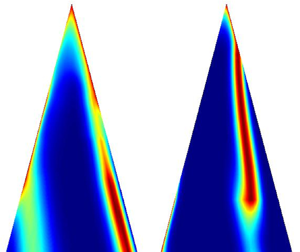
Figure 2 shows the variation of  $\rho (\tau \,|\,\phi )$ for four initial stimulus phases, $\phi =0$, ${\rm \pi} /2$, ${\rm \pi}$, $3{\rm \pi} /2$. Panels in each row (from the top) correspond to harmonic excitation amplitudes $A=0.4$, 0.2 and $0$, while panels in each column (from the left) represent noise amplitudes $A_n=0.05$, 0.2 and $0.4$. All the PDFs show a set of exponentially decaying functions. The peaks are located away from the natural vortex shedding time period ( $\tau =1$) at the combination of the highest harmonic excitation amplitude and the lowest noise amplitude (figure 2(a), $A=0.4$, $A_n=0.05$). The peaks deteriorate as one decreases $A$ (along the columns) or increases $A_n$ (along the rows). The first row panels show a strong dependence of $\rho$ on the initial stimulus phase $\phi$, showing the non-stationary behaviour of the shedding process due to the harmonic excitation. As $A$ is reduced, all $\rho$ corresponding to various $\phi$ approach each other. In fact, at $A=0$ (last row), the dependency on $\phi$ vanishes completely, making the process stationary. An analytical solution for $\rho$ at $A=0$ is available from Molini et al. (Reference Molini, Talkner, Katul and Porporato2011):
 \begin{equation} \rho (\tau)=\frac{1}{\sqrt{8{\rm \pi}}\,A_n\tau^{3/2}}\exp {\left[-\frac{(\tau-1)^2}{8A_n^2\tau}\right]}. \end{equation}
The above expression is plotted as grey points in figures 2(g–i). At the lowest noise  $A_n=0.05$ (figure 2g), $\rho$ is centred close to $1$, indicating that vortex shedding occurs at its deterministic natural frequency (1 in our case). As $A_n$ increases (figures 2g–i), the peak drops (as expected), and shifts to lower values of $\tau$ (less than 1). The physical reasoning for the latter is as follows. The formal solution of (2.1) is
 \begin{equation} \varGamma (\tau)=\int_{\tau^*=0}^{\tau^*=\tau}\frac{[1+u(\tau^*)]^2}{2}\,{\rm d}\tau^* +A_n\int_{\tau^*=0}^{\tau^*=\tau}\eta(\tau^*)\,{\rm d}\tau^*. \end{equation}
This solution is used to construct an expression for the ensemble average (angular brackets) of  $\varGamma ^2$:
 \begin{equation} \langle \varGamma^2(\tau)\rangle =\left(\int_{\tau^*=0}^{\tau^*=\tau}\frac{[1+u(\tau^*)]^2}{2}\,{\rm d}\tau^*\right)^2+A_n^2\tau. \end{equation}
The first and second terms on the right-hand side represent the contributions of deterministic (harmonic) and stochastic excitations, respectively. In particular, noise strictly increases the value of  $\langle \varGamma ^2\rangle$, thereby allowing the condition $\varGamma =\varGamma _{sep}$ for vortex shedding to be reached more quickly (in the sense of ensemble average) than its deterministic counterpart (when $A_n=0$). Therefore, the noise tends to push the system to take lower shedding periods. The above effect leads to the reasoning of asymmetric reduction in the lock-in region due to noise (see § 3.1). Expression (2.19) is valid and therefore the reasoning for the Gaussian white noise only.

Figure 2. Variation of conditional PDF for vortex shedding time interval  $\rho (\tau \,|\,\phi )$ at four stimulus phases, $\phi =0$, ${\rm \pi} /2$, ${\rm \pi}$, $3{\rm \pi} /2$, excited by harmonic excitations of amplitudes (a–c) $A=0.4$, (d–f), $A=0.2$, and (g–i), $A=0$. Three noise amplitudes are considered: (a,d,g) $A_n=0.05$, (b,e,h) $A_n=0.2$, and (c,f,i) $A_n=0.4$. Excitation frequency is kept at $f=0.8$. The grey lines in (g–i) show the analytical results from Molini et al. (Reference Molini, Talkner, Katul and Porporato2011), which are valid for $A=0$.
2.2. Step 2: assembly of the vortex shedding events
We now proceed to the next step, where we assemble the shedding events to obtain the spike train  $f(t)$. As said before, $\rho (\tau \,|\,\phi )$ gives the PDF of the vortex shedding time period, given the phase of the last shedding $\phi$. The phase of the current shedding is therefore $\psi =(\omega \tau +\phi )\ {\rm modulo}\ 2{\rm \pi}$. At this point, it is convenient to move the shedding period distribution quantified in terms of time $\tau$ to phase $\psi$. This allows us to wrap the sample space from $[0,\infty )$ to $[0,2{\rm \pi} ]$, a move performed in the deterministic case too (Britto & Mariappan Reference Britto and Mariappan2019, Reference Britto and Mariappan2021). The PDF $\mathscr {T}(\psi \,|\,\phi )$ in terms of $\psi$ reads
 \begin{equation} \mathscr{T}(\psi\,|\,\phi)=\int_0^\infty \rho(\tau\,|\,\phi)\,\delta(\psi-(\omega \tau+\phi)\ {\rm modulo}\ 2{\rm \pi})\frac{{\rm d}\tau}{\omega}, \end{equation}
where  $\mathscr {T}$ is termed the transition probability of the shedding (spike) phase to occur at $\psi$ given that $\phi$ is the shedding phase of the last shedding. We now perform the assembly of the shedding phase $\psi _m$. Consider an ensemble of experiments, where individual realizations begin with a given initial phase $\phi$. Let this have a PDF given by $\chi ^0(\phi )$ (where superscript $0$ indicates the initial instant). The phase distribution $\chi ^1(\psi )$ at the end of the first vortex shedding is therefore $\mathscr {T}(\psi \,|\,\phi )\,\chi ^0(\phi )$, ensembled over the sample space of $\phi$, namely $[0,2{\rm \pi} ]$. Consequently, the phase distribution PDFs of the $(m+1)$th and $m$th vortex sheddings are related as follows:
 \begin{equation} \chi^{m+1}(\psi)=\int_0^{2{\rm \pi}}\mathscr{T}(\psi\,|\,\phi)\,\chi^m(\phi)\,{\rm d}\phi. \end{equation}
Note that  $\phi$ and $\psi$ can be regarded as a stimulus and response phase, respectively, for the $(m+1)$th vortex shedding process. Since the $(m+1)$th phase distribution depends only on the previous ( $m$th) distribution, the shedding process (spike train) quantified through phase also follows a Markov process. Furthermore, the initial phase distribution $\chi ^0(\phi )$ determines completely the time evolution of the train. In order to remove the effect of the initial condition and make predictions that can be verified through experiments, it is imperative to analyse the asymptotic behaviour of the spike train $f(t)$ (i.e. $t\rightarrow \infty$). As mentioned in the literature (Plesser & Geisel Reference Plesser and Geisel1999; Tateno & Jimbo Reference Tateno and Jimbo2000), $\chi ^m$ reaches a unique stationary phase distribution $\chi ^s$ in the limit $m\rightarrow \infty$, which is independent of the initial condition $\chi ^0(\phi )$. This is guaranteed when $\mathscr {T}(\psi \,|\,\phi )>0$ for all $\psi,\phi$ (Tateno & Jimbo Reference Tateno and Jimbo2000). Through numerical simulations in this work, we observe that the above condition is satisfied.
The stationary phase distribution can be obtained by replacing both  $\chi ^m$ and $\chi ^{m+1}$ with $\chi ^s$ in (2.21), and solving the integral equation for $\chi ^s$. Since $\rho$ and therefore $\mathscr {T}$ are obtained numerically, (2.21) is also solved numerically by discretizing the integral and $\phi,\psi$ into $L+1$ bins (in this paper $L=100$) having width $\Delta \phi =\Delta \psi =2{\rm \pi} /L$. In the discretized form, $\boldsymbol {\phi }=(\phi _1,\phi _2,\ldots,\phi _{L+1})^{\rm T}$, $\boldsymbol {\psi }=(\psi _1,\psi _2,$ $\ldots,\psi _{L+1})^{\rm T}$ and ${\boldsymbol {\chi }}=(\chi _1=\chi (\psi _1),\chi _2=\chi (\psi _2),\ldots,\chi _{L+1}=\chi (\psi _{L+1}))^{\rm T}$, with $\phi _j=\psi _j$ $=\Delta \phi \,(j-1)$. Since by construction $\chi$ is $2{\rm \pi}$ periodic, $\chi _1= \chi _{L+1}$. Equation (2.21) thus becomes the following, after applying the trapezoidal rule to the integral and enforcing the periodic boundary condition:
 \begin{equation} \chi_k^{m+1}=\Delta \phi\sum_{j=1}^{L}\mathscr{T}(\psi_k\,|\,\phi_j)\,\chi_j^m,\quad k=1,2,\ldots L, \end{equation}
or in matrix form,
 \begin{gather} \boldsymbol{\chi^{m+1}}=\boldsymbol{T}\boldsymbol{\chi^{m}},\quad \boldsymbol{T}=[T]_{kj}=\mathscr{T}(\psi_k\,|\,\phi_j)\,\Delta \phi.\end{gather}
 The discretized stationary distribution  $\boldsymbol {\chi ^s}$ therefore becomes the eigenvector of the matrix $\boldsymbol {T}$ having eigenvalue 1. The other eigenvalues are, in general, complex, having absolute value less than 1. They are used to characterize stochastic bifurcation occurring in this system (detailed in § 3). The last step is to calculate the PDF of the vortex shedding time interval $\rho _s$, corresponding to the stationary stimulus phase distribution $\chi ^s$:
 \begin{equation} \rho_s(\tau)=\int_0^{2{\rm \pi}}\rho(\tau\,|\,\phi)\,\chi^s(\phi)\,{\rm d}\phi. \end{equation}
 The results of the above assembly process are illustrated through figures 3 and 4. We begin with the former figure, where plots of the discretized transition probability matrix  $\boldsymbol {T}$ (figures 3a,d), its eigenvalues $\kappa$ (figures 3b,e) and the evolution of $\chi ^m$ from a random initial distribution $\chi ^0$ (figures 3c,f) for two harmonic excitation amplitudes $A=0.2$ (figures 3a–c) and $A=0$ (figures 3d–f) are shown. Excitation frequency and noise amplitude are kept at $f=0.9$ and $A_n=0.02$, respectively. As interpreted from (2.23), $\boldsymbol {T}$ acts as a propagator matrix to map the system from the $m$th to the $(m+1)$th shedding events. Therefore, the columns and rows of $\boldsymbol {T}$ can be associated with $\chi ^m$ (stimulus phase $\phi$) and the response $\chi ^{m+1}$ (response phase $\psi$). At $A=0.2$ (figure 3a), the entries of $\boldsymbol {T}$ show dominant values near $\psi /{\rm \pi} =1$. This indicates that for most of the values of the present shedding phase $\chi ^m$, the next shedding occurs mostly around $\chi ^{m+1}/{\rm \pi} =1$. Therefore, after applying $\boldsymbol {T}$ multiple times, the obtained stationary distribution $\chi ^s$ is expected to have a peak in its distribution around ${\rm \pi}$, which is found to occur as shown in figure 3(c) (red curve). The spectrum of $\kappa$ (figure 3b) shows that the largest eigenvalue is indeed $1$, with the other eigenvalues lying inside the unit circle (black curve). Figure 3(c) shows that within a few iterations ( $m=15$), $\chi ^m$ from a random distribution ends up as $\chi ^s$.

Figure 3. (a,d) Contour plot of the discretized transition probability matrix  $\boldsymbol {T}$. The dashed white line represents the main diagonal. Blue and red colours indicate minimum and maximum values respectively. (b,e) Eigenvalues $\kappa$ of $\boldsymbol {T}$. The black curve indicates the unit circle. (c,f) Fifteen iterates of $\chi ^m$ starting from $\chi ^0$, having a random distribution; $\chi ^0$ and $\chi ^{15}$ are marked in blue and red, respectively. The intermediate states $\chi ^m$ ( $0< m<15$) are also shown, with the arrow direction marking the evolution in $m$. Panels (a–c) correspond to $A=0.2$, and (d–f) to $A=0$. Other parameter values are fixed at $f=0.9$ and $A_n=0.02$.

Figure 4. (a) Stationary phase distribution  $\chi ^s$, and (b) stationary vortex shedding time interval $\rho _s$, for three harmonic excitation amplitudes $A=0, 0.045, 0.2$, with $f=0.9$ and $A_n=0.02$.
Figures 3(d–f) show the same plots corresponding to  $A=0$. Dominant entries of $\boldsymbol {T}$ (figure 3d) are along its main diagonal (dashed white line). By shifting suitably the $\phi$-axis, it is possible to make these dominant entries align exactly with the main diagonal. Therefore, unlike the previous case ( $A=0.2$), for every current shedding phase $\chi ^m$, the next shedding phase $\chi ^{m+1}$ occurs with equal probability in the sample space $[0,2{\rm \pi} ]$. Thus the stationary distribution $\chi ^s$ is a uniform distribution. The iterates $\chi ^m$ indeed converge to a uniform distribution (figure 3f). At zero harmonic excitation, the presence of noise ( $A_n\neq 0$) does not alter the asymmetry associated with the shedding phase. All the shedding phases are equally probable and lead to uniform $\chi ^s$.
Corresponding to the stationary phase distribution, the PDF of the vortex shedding interval is shown in figure 4. Once again,  $\chi ^s$ is plotted in figure 4(a) for clarity ( $A=0$, $0.045$ and $0.02$, and other parameters are the same as in figure 3) and the corresponding $\rho _s$ in the adjacent panel (figure 4b). In the absence of harmonic excitation ( $A=0$), one expects vortex shedding to occur mostly at the natural shedding frequency $1$ with a spread determined by $A_n$ (red curve in figure 4b). As $A$ increases, the peak shifts to the right (refer to the blue curve corresponding to $A=0.045$). At $A=0.2$, the peak occurs at $\tau =1.11=1/f$, indicating that it has locked to the stimulation frequency. We now observe a 1 : 1 phase lock-in, but in the stochastic sense. As a counterpart of the deterministic case ( $A_n=0$), a stochastic bifurcation occurs, leading to lock-in. The occurrence of stochastic bifurcation is identified by a qualitative change in the spectrum of $\boldsymbol {T}$ (Doi, Inoue & Kumagai Reference Doi, Inoue and Kumagai1998). The details are presented in the next section.
3. Stochastic bifurcation
Stochastic bifurcation analysis is conducted at three excitation frequencies,  $f=0.9$, $3.2$ and $0.6$, which are close to the fundamental, superharmonic and subharmonic of the natural vortex shedding frequency, respectively. A detailed deterministic bifurcation analysis was performed for $f=0.9$ and $3.2$ in our earlier paper (Britto & Mariappan Reference Britto and Mariappan2019), which motivated us to choose the above frequencies for the present investigation. Furthermore, the results discussed are qualitatively the same, between the excitations on either side of the fundamental/subharmonic/superharmonic of the natural vortex shedding frequency. Hence we choose $f=0.6$ to describe the dynamics associated with subharmonic excitation.
3.1. Fundamental excitation
Panels in figure 5 describe the stochastic bifurcation dynamics with the harmonic excitation amplitude  $A$ as the bifurcation parameter, excited with harmonic frequency $f=0.9$ and noise amplitude $A_n=0.02$. Figure 5(a) shows the deterministic ( $A_n=0$) bifurcation diagram, which serves as our reference. Time intervals ( $\tau$) between successive sheddings for a total of 1000 iterates (after discarding the transients) are plotted. At $A=0$, vortices are shed at their natural shedding frequency. As $A$ increases, the shedding becomes quasi-periodic, marked by the iterates filling a finite $\tau$ region densely. At $A=0.12$, saddle-node bifurcation occurs, leading to 1 : 1 phase lock-in (deterministic). Vortices are now shed at the forcing time period ( $\tau =1/f=1.11$). This lock-in continues up to $A=0.75$, where a transition to a higher periodic solution occurs. For $A\geq 0.83$, a period-2 orbit forms, where vortex shedding time instances occur between the values $\tau \sim 0.8$ and $\tau \sim$ 0.3 alternately. The mean shedding time period $(\mu _{\tau })$ at each amplitude is plotted as a blue curve in figure 5(b). In the region of the period-2 orbit, $\mu _{\tau }=1/2f$. This indicates that for completing one period-2 orbit (two vortex sheddings), a total time of $1/f$ is required, which equals the time period of harmonic excitation. Two cycles of vortex shedding (response) correspond to one harmonic excitation cycle. Therefore, shedding exhibits 1 : 2 phase lock-in with the excitation. Furthermore, abrupt changes in $\mu _{\tau }$ are observed at the ends of lock-in and higher periodic orbit regimes. The above are the characteristics of deterministic bifurcations.

Figure 5. (a) Plot showing 1000 iterates of the instantaneous vortex shedding time period  $\tau$ for the deterministic case ( $A_n=0$). Iterates forming the horizontal line represent the extent of deterministic 1 : 1 phase lock-in. (b) Variation of mean ( $\mu _{\tau }$) and standard deviation ( $\sigma _{\tau }$) of $\tau$ with harmonic excitation amplitude $A$. The blue curve represents the mean $\tau$ of the deterministic case. Grey portions indicate the stochastic 1 : 1 and 1 : 2 phase lock-in regions (labelled as s-lock-in). Variations of stationary PDFs correspond to (c) vortex shedding time period $\rho _s$, and (d) phase distributions $\chi ^s$, with $A$. Vertical white and red lines indicate the extents of the stochastic 1 : 1 and 1 : 2 phase lock-ins, respectively. Variation of the first three eigenvalues $\kappa _q$ with $A$: (e) absolute value, and (f) phase. Variation of the second (g,h) and third (i,j) eigenvectors ( $\boldsymbol{v}_q$) of $\boldsymbol {T}$ with $A$: imaginary part (g,i), and real part (h,j). Black and red vertical lines represent the extents of the 1 : 1 and 1 : 2 stochastic lock-ins, respectively. The other parameters are $f=0.9$, $A_n=0.02$.
In the presence of noise ( $A_n=0.02$), the mean ( $\mu _{\tau }$) and standard deviation ( $\sigma _{\tau }$) of the shedding time interval, calculated from the stationary distribution $\rho _s$, are plotted (figure 5b). Similar to the deterministic case, $\mu _{\tau }$ becomes flat, with values $1/f$ and $1/2f$ in 1 : 1 and 1 : 2 phase lock-in regions, but the transition is more gradual than in the deterministic case. This feature indicates that the system exhibits lock-in behaviour, albeit in the stochastic sense. Moreover, in the regions where $\mu _{\tau }$ stays flat, the corresponding $\sigma _{\tau }$ shows a local dip, further emphasizing the increased repeatability of the shedding occurrences during s-lock-in.
In the deterministic case, the occurrence of lock-in is identified by a saddle-node bifurcation (Britto & Mariappan Reference Britto and Mariappan2019), where two new solutions (one stable and the other unstable) emerge. The stable solution corresponds to lock-in. In the stochastic analogue, the bifurcation (p-bifurcation as referred to in Arnold Reference Arnold1995) is characterized by a qualitative change in the stationary PDF of an appropriate random variable, in this case  $\rho _s$ for $\tau$.
Figure 5(c) shows the stationary time interval distribution  $\rho _s$ for various $A$. The distribution peaking at $\tau =1$ for $A=0$ transitions its peak to $\tau =1/f$ for $A>0.21$. Also, for large $A$ (
$A$ ( $A>0.6$), two more peaks emerge, having crests at $\tau \sim 0.8$ and $\tau \sim 0.3$ (similar to the deterministic case). A qualitative change in $\rho _s$ is observed: a unimodal distribution changes to a trimodal distribution at $A=0.6$, which hints at the occurrence of (stochastic) bifurcation. Further, at $A=0.75$, the trimodal distribution switches to a bimodal one. These changes are gradual. Although qualitative changes occur in $\rho _s$, they do not corroborate the occurrence of a flat mean vortex shedding period $(\mu _{\tau })$ (see figure 5b). A similar conclusion appears while analysing the stationary phase distribution $\chi ^s$ (figure 5d). Therefore, in the present system, the occurrence of lock-in (stochastic bifurcations) cannot be identified solely by the stationary probability distributions, which describe the asymptotic state of the system.
Alternatively, qualitative changes in the dynamics of the system on its route to the stationary distribution can identify stochastic bifurcations. As we said in § 2.2, (2.23) describes the evolution of the system, where the propagator matrix  $\boldsymbol {T}$ contains all the information of the dynamics. Writing (2.23) in the eigenvector basis of $\boldsymbol {T}$ leads to
 \begin{gather} \chi^{m+1}=\boldsymbol{T}^m\chi^0=\sum_{q=1}^Lc_q\kappa_q^m \boldsymbol{v}_q, \end{gather}
 \begin{gather}\text{initial condition,}\quad\chi^0=\sum_{q=1}^Lc_q \boldsymbol{v}_q, \end{gather}
where  $\kappa _q$ and $\boldsymbol {v}_q$ represent the $q$th eigenvalue and its eigenvector of $\boldsymbol {T}$, respectively. Eigenvalues are arranged in descending order of their absolute values. The initial condition $\chi ^0$ is expressed in the eigenbasis of $\boldsymbol {T}$, where $c_q$ are the associated projection coefficients. Equation (3.1) shows that the contribution of an eigenvector to the evolution of $\chi ^{m+1}$ depends on the absolute value of its eigenvalue. We know that the first (largest) eigenvalue is 1 and the corresponding eigenvector is the stationary phase distribution $\chi ^s$ to which the system evolves as $m\rightarrow \infty$. The next eigenvalues (second and third) determine the evolution path taken by the system on its journey to reach $\chi ^s$.
Stochastic bifurcation is identified by tracking the spectrum of  $\boldsymbol {T}$ (Doi et al. Reference Doi, Inoue and Kumagai1998). The absolute value and phase of the first three eigenvalues ( $\kappa _1,\kappa _2,\kappa _3$) are plotted in figures 5(e,f), respectively. As $A$ increases, at $A=0.21$, the second ( $\kappa _2$) and third ( $\kappa _3$) eigenvalues transition from being complex conjugates to real. They remain real until $A=0.42$. Since $\theta _{\kappa _{q}}=0$ for $q=2, 3$, $\boldsymbol {T} \boldsymbol{v}_q=\kappa _q \boldsymbol{v}_q=|\kappa _q| \boldsymbol{v}_q$ which indicates that $\boldsymbol{v}_q$ is invariant under the action of $\boldsymbol {T}$ with an amplitude decay $|\kappa _q|$. The corresponding eigenvectors $v_2,v_3$ do become real in the amplitude range $0.21\leq A \leq 0.42$ (figures 5g,i). Therefore, the system is said to exist in a 1 : 1 phase lock-in (stochastic sense) state with the harmonic excitation. The extent of this lock-in is shown as grey regions in figures 5(b), and white and black vertical lines in figures 5(c,d,g–j). Since the second and third eigenvalues are the dominant eigenvalues next to the largest (first) eigenvalue, their change in behaviour manifests as 1 : 1 lock-in in $\mu _{\tau }$ (figure 5b).
The occurrence of 1 : 2 lock-in between  $A=0.79$ and $A=0.96$ can also be explained through the spectrum. In the above range, the absolute value of the second eigenvalue approaches the first eigenvalue ( $|\kappa _2|\rightarrow |\kappa _1|=1$; figure 5e). Furthermore, its phase becomes $\theta _2={\rm \pi}$ (figure 5f). Therefore, $\boldsymbol {T}^2 v_2=\kappa _2 v_2=|\kappa _2|^2 v_2$, indicating that the dynamics (up to second eigenvalue) remains invariant after propagating two vortex shedding cycles. This time there is an insignificant amplitude decay since $|\kappa _2|$ is close to 1. Therefore, the stationary stochastic state $\rho _s$ alternates (mostly) between two states (period-2 orbit). The corresponding stationary distribution is therefore bimodal. Note that the second eigenvector in this amplitude range becomes real (figures 5g,i). A linear combination of the first two eigenvectors determines the stationary distribution. The extent of 1 : 2 lock-in is marked by red vertical lines in figures 5(c,d,g–j).
Noise in (2.1) is additive. Therefore, the underlying dynamical features such as period-1, period-2 and higher-period solutions remain the same as for their deterministic counterparts. Since noise is disruptive, its presence reduces the extent of 1 : 1 lock-in. The reduction on either side is asymmetric. In 1 : 1 lock-in, the reduction is more on the higher amplitude ( $A$) side than on the lower side, which can be explained as follows. Along with the disruptive nature, the presence of noise is to reduce the mean shedding time period $\tau$ (as evident from $A=0$ simulations shown in figure 2g–i). Therefore, noise pushes the system frequently towards the dynamics containing smaller $\tau$. Near the lower threshold of 1 : 1 deterministic lock-in ( $A=0.12$), the mean $\tau$ increases as the system moves from quasi-periodic to lock-in region (figure 5b). Both the disruptive and lowering mean $\tau$ nature of noise work in opposition, leading to a smaller reduction in the extent of the lower 1 : 1 lock-in region. Near the upper threshold side ( $A=0.75$), the mean $\tau$ of the system decreases sharply (figure 5b). Therefore, both the above effects are favourable for a quick end to the lock-in region. The presence of the higher-periodic solution is felt as a multimodal PDF in $\tau$ as early as $A=0.65$ (figure 5c).
To summarize, a qualitative change in the stationary PDF is not observed to identify the onset and end of s-lock-in. The first three eigenvalues of the discretized transition probability matrix determine the system evolution and hence the stochastic bifurcations. In particular, the phase of the eigenvalue determines the order and extent of s-lock-in. The closeness of its amplitude to 1 dictates the coincidence of the mean shedding period with the excitation time period. The above bifurcation scenario is valid on the other frequency side,  $f>1$, too. During combustion instability, several investigations indicated that apart from the fundamental acoustic mode, higher modes or combinations are excited (Lieuwen Reference Lieuwen2003; Kabiraj & Sujith Reference Kabiraj and Sujith2012). Therefore, it is imperative to study lock-in when the excitation is close to the superharmonic and subharmonic of the natural vortex shedding frequency.
3.2. Superharmonic excitation
We consider the excitation frequency  $f=3.2$ near the (third) superharmonic of the natural vortex shedding frequency. The results are shown in figure 6. Going through the deterministic scenario (figure 6a), as $A$ is increased ( $A>0.065$), vortex shedding first locks to the closest (third) subharmonic of the excitation frequency, establishing 3 : 1 lock-in (ratio of forcing to response frequency is 3). At higher amplitudes ( $A>0.30$), shedding locks out of the excitation frequency and cascades to lock-in ( $A>0.34$) with the second subharmonic of the excitation frequency (2 : 1 lock-in). A third cascade occurs for $A>0.63$ to establish 1 : 1 lock-in. Details of the mechanism causing this cascade from 3 : 1 to 1 : 1 lock-in are discussed in Britto & Mariappan (Reference Britto and Mariappan2019). The average of the iterates (blue curve in figure 6b) shows sudden variation at the onset and end of lock-in regions. In the transition between 3 : 1 and 2 : 1 lock-in, period-2 solution occurs for $0.30\leq A \leq 0.33$ (figure 6a). Their average time period is $5/2f$ (figure 6b), indicating the occurrence of 5 : 2 lock-in. Similarly, 3 : 2 lock-in is observed for $0.61 \leq A \leq 0.63$ in the transition between 2 : 1 and 1 : 1 lock-in regions.

Figure 6. (a) Plot showing 1000 iterates of the instantaneous vortex shedding time period  $\tau$ for the deterministic case ( $A_n=0$). Iterates forming the horizontal line represent the extent of deterministic phase lock-in. (b) Variation of mean ( $\mu _{\tau }$) and standard deviation ( $\sigma _{\tau }$) of $\tau$ with harmonic excitation amplitude $A$. The blue curve represents the mean $\tau$ of the deterministic case. Variation of the first three eigenvalues $\kappa _q$ with $A$: (c) absolute, and (d) phase. Variation of stationary PDFs corresponding to: (e) vortex shedding time period $\rho _s$, and (f) phase distributions $\chi ^s$ with $A$. Vertical red, green, yellow, magenta and white lines indicate the extent of stochastic 3 : 1, 5 : 2, 2 : 1, 3 : 2 and 1 : 1 s-lock-ins, respectively. Other parameters are $f=3.2$, $A_n=0.02$.
As before, mean  $\mu _{\tau }$ and standard deviation $\sigma _{\tau }$ corresponding to the stationary shedding time period (with noise $A_n=0.02$, as in § 3.1) are plotted in figure 6(b). The curve of $\mu _{\tau }$ does not flatten near the deterministic 3 : 1 and 2 : 1 lock-in regions, indicating the (apparent) absence of their stochastic counterparts. Flattening of $\mu _{\tau }$ at $1/f$ is observed, showing the possibility of stochastic 1 : 1 phase lock-in. Furthermore, the standard deviation $\sigma _{\tau }$ also hits a trough in this region.
Figures 6(c) (absolute) and 6(d) (phase) show the variation of the first three eigenvalues with  $A$. The phase of the second eigenvalue becomes $\theta _2=0$ in the amplitude regions $0.1< A<0.13$, $0.38< A<0.46$ and $0.69< A<0.92$, showing the occurrence of a general $p$ : 1 ( $p$ integer) s-lock-in. This $p$ is identified from the peak location in the PDF of $\tau$ (figure 6e). Out of the three lock-in regions (3 : 1, 2 : 1 and 1 : 1), the last one has the largest amplitude range, marking the extent of 1 : 1 s-lock-in. In the initial portion of this lock-in region, $\mu _{\tau }$ is not yet flat ( $0.69< A<0.76$). The reason is that the absolute value of $\kappa _q$ of the second (and higher) eigenvalue is much smaller than the first eigenvalue (note the log scale for $|\kappa _q|$ in figure 6c). Therefore, though a qualitative change in the second eigenvalue occurs, its influence on the dynamics is weak. Similarly, stochastic 3 : 1 and 2 : 1 lock-ins do occur in the amplitude regions $0.1< A<0.13$ and $0.38< A<0.46$, respectively. However, a corresponding flatness in $\mu _{\tau }$ is not observed, which poses a difficulty in experimental measurements to identify lock-in regions in the presence of background noise. Therefore, apart from $\mu _{\tau }$, the PDF of $\tau$ should be obtained, which shows local peaks at $1/pf$, marking the existence of $p$ : 1 s-lock-in (figure 6e). Similar to § 3.1, a qualitative change in $\rho _s$ (number and location of peaks) is observed in the cascade from 3 : 1 to 1 : 1 lock-in (panel $c$). Multiple peaks indicate that the system spends time partly in two different lock-in regions (for example, at $A=0.25$, shedding occurs mostly at $1/3f$ and $1/2f$ time periods), which poses difficulty in the classification of lock-in order. The above point emphasizes further the use of the spectrum of $\boldsymbol {T}$ in the identification of the occurrence and order of s-lock-in. Since the stationary phase distribution ( $\chi ^s$, figure 6f) is wrapped in $[0,2{\rm \pi} ]$, the qualitative change during the cascade is more subtle. It shares the same disadvantage as $\rho _s$ in the identification of s-lock-in.
Apart from the  $p$ : 1 s-lock-in, stochastic counterparts of 5 : 2 and 3 : 2 lock-in are observed ( $\theta _2={\rm \pi}$) in figure 6(d). These s-lock-in regions occur for $0.24\leq A \leq 0.29$ and $0.52\leq A \leq 0.60$, respectively. They serve as smooth transition zones from 3 : 1 to 2 : 1, and from 2 : 1 to 1 : 1 s-lock-in regions, respectively.
3.3. Subharmonic excitation
Similarly to the previous case, the dynamics of vortex shedding excited at a frequency close to the first subharmonic of the natural shedding frequency is illustrated through figure 7. Deterministic 1 : 2 lock-in occurs in  $0.49< A<0.97$. In the amplitude range $0.48< A<0.85$, (i) the absolute value of the second eigenvalue, $|k_2|$, approaches 1 (figure 7c), and (ii) its phase angle becomes ${\rm \pi}$ (figure 7d). These two points indicate the occurrence of 1 : 2 s-lock-in. The corresponding PDF of $\tau$ (figure 7b) shows bimodal distribution. Beyond the 1 : 2 s-lock-in region, $|k_2|$ and $|k_3|$ become close to 1 at $A=0.97$. Their corresponding phases become $\pm 2{\rm \pi} /3$, marking the presence of 1 : 3 s-lock-in. It is reflected as a trimodal distribution for $\tau$ at $A=0.97$. Immediately beyond $A=0.97$, the phase drops suddenly, showing the narrow region of 1 : 3 s-lock-in.

Figure 7. (a) Plot showing 1000 iterates of the instantaneous vortex shedding time period  $\tau$ for the deterministic case ( $A_n=0$). (b) Variation of PDF of $\tau$ with harmonic excitation $A$. Vertical white lines indicate the extent of 1 : 2 s-lock-in. Variation of the first three eigenvalues $\kappa _q$ with amplitude: (c) absolute, and (d) phase. Other parameters are $f=0.6$, $A_n=0.02$.
4. Noise-induced dynamics
The previous section discussed identifying s-lock-in using the spectrum of the transition probability matrix. The amplitude of the harmonic excitation  $A$ was the bifurcation parameter. In this section, the noise amplitude $A_n$ is set as the bifurcation parameter at various $A$. We observe the following. (1) Addition of noise disrupts lock-in. (2) An increase in noise amplitude $A_n$ promotes the system towards the states having lower shedding periods. (3) There is stochastic resonance where there is an occurrence of non-monotonic amplification of the input harmonic signal by the noise. The results are illustrated in figure 8. Here, $A_n$ is varied between $5\times 10^{-3}$ and 0.2. The excitation frequency is set to $f=0.9$. Each row corresponds to a particular harmonic amplitude $A\in \{0.1,0.25,0.6,0.75,0.8\}$, associated with different dynamical behaviour of the deterministic case (figure 5a). Each row contains three columns: (i) left, stationary PDF ( $\rho _s$) of $\tau$; (ii) middle, mean ( $\mu _{\tau }$) and standard deviation ( $\sigma _{\tau }$) of $\tau$, along with the horizontal lines at $1/f$ (red) and $1/2f$ (green); and (iii) right, absolute value (blue) and phase (red) of the second eigenvalue $\kappa _2$, which decides the occurrence and order of s-lock-in.

Figure 8. Illustration of noise induced dynamics. Noise amplitude is varied from  $5\times 10^{-3}$ to 0.2 at various harmonic amplitudes $A=0.1$ (a–c), $A=0.25$ (d–f), $A=0.6$ (g–i), $A=0.75$ (j–l), and $A=0.8$ (m–o). Each row contains three columns: (i) left, stationary PDF ( $\rho _s$) of $\tau$; (ii) middle, mean and standard deviation of $\tau$, along with the horizontal lines at $1/f$ (red) and $1/2f$ (green); and (iii) right, absolute value (blue) and phase (red) of the second eigenvalue $\kappa _2$. The excitation frequency is set at $f=0.9$.
The first and expected observation to make is that the increase of noise  $A_n$ leads to smear in the PDF $\rho _s$ (figures 8a,d,g,j,m), which manifests as an inflation in $\sigma _{\tau }$. At $A=0.1$, the deterministic system exhibits quasi-periodic shedding. The corresponding shedding time period PDF shows a unimodal distribution with the peak occurring at $\tau$ close at the natural shedding period ( $\tau =1$). At the next higher excitation amplitude $A=0.25$, 1 : 1 lock-in occurs in the deterministic case. Stochastic 1 : 1 lock-in also takes place, which is evident from (i) the peak in $\rho _s$ occurring at $\tau =1/f$ (figure 8d), (ii) the mean shedding period $\mu _{\tau }$ coinciding with $1/f$ (figure 8e), and (iii) the phase $\theta _{\kappa _2}$ becoming zero (figure 8f), all occurring at $A_n=5\times 10^{-3}$. Increase in $A_n$ disrupts lock-in.
At  $A=0.6$, while deterministic 1 : 1 lock-in prevails, s-lock-in ceases to exist even at the lowest considered noise amplitude ( $\theta _{\kappa _2}$ starts and drifts away from zero). Apart from non-zero probability concentrated near $\tau =1/f$, two more regions ( $\tau \sim 0.8, 0.3$) sprout and become stronger at large $A_n$ (figure 8g). These two regions correspond to the iterates of 1 : 2 lock-in, observed at $A\geq 0.83$ of the deterministic case. As said earlier, the increase in $A_n$ pushes the system to take states having lower values of $\tau$. In the present case, these states occur at higher amplitudes $A$ (see figure 5b). Thus noise prepones the dynamics (observed at higher amplitudes in the deterministic case) to lower harmonic amplitudes $A$. The amount of preponement increases with an increase in $A_n$. In fact, $\theta _{\kappa _2}$ becomes ${\rm \pi}$ for $A_n>0.18$ (figure 8i) indicating the occurrence of 1 : 2 s-lock-in. Since $|\kappa _2|$ is much lesser than 1, this s-lock-in is not reflected in $\mu _{\tau }$. However, $\mu _{\tau }$ approaches $1/2f$ (figure 8h) with increase in $A_n$.
At  $A=0.75$ (marking the end of deterministic 1 : 1 lock-in), the distribution near $\tau =1/f$ becomes weaker, while that near the period-2 solution grow stronger (figure 8j). There is a rise in the extent of 1 : 2 lock-in, with values of $|\kappa _2|$ closer to 1 (figure 8l). Then $\mu _{\tau }$ hovers in the neighbourhood of $1/2f$ (figure 8k). Something non-trivial occurs at the largest considered amplitude, $A=0.8$. The PDF near $\tau =1$ vanishes for low and high $A_n$, while having an island peak for intermediate values $A_n=0.05\unicode{x2013}0.14$. This indicates an increased probability for the vortices to shed at the excitation frequency on this island. The corresponding $\mu _{\tau }$ also shows a bulge owing to the large shedding time period associated with the island (figure 8n). Therefore, the response of the system at the excitation frequency elevates at these intermediate noise amplitudes, suggesting the occurrence of stochastic resonance.
4.1. Stochastic resonance
Stochastic resonance (SR) is a phenomenon where the presence of noise amplifies the response of the system to an input signal. In this paper, harmonic velocity excitation  $u$ is the input signal. The response is the circulation of the shed vortex $\varGamma _v$ at the input signal frequency. This variable is relevant, as heat energy transported by the vortex is proportional to its circulation, a relation used in the original model (Matveev & Culick Reference Matveev and Culick2003) and later investigations (Tulsyan, Balasubramanian & Sujith Reference Tulsyan, Balasubramanian and Sujith2009). An expression for $\varGamma _v$ is
 \begin{equation} \varGamma_v(t)=\sum_{m=0}^{\infty} \delta(t-t_m)\,\varGamma_{sep}(t). \end{equation}
As before,  $t_m$ represents the vortex shedding instant. A spike in circulation is observed as and when a vortex is shed; $\varGamma _v$ is also a random variable. Stochastic resonance is identified by tracking the quantity signal-to-noise ratio (SNR). It is defined as the ratio of power in the response to noise at the forcing frequency $\omega$. The one-sided power spectral density (PSD) of $\varGamma _v$ at $\omega$ in the observation time $T_{0}$ is defined as (Priestley Reference Priestley1981)
 \begin{align} S_{\varGamma}(\omega)&=\frac{1}{{\rm \pi} T_0}\left\langle \left| \int_0^{T_0} \varGamma_v \,{\rm e}^{{\rm i}\omega t}\,{\rm d}t\right|^2\right\rangle =\frac{1}{{\rm \pi} T_0}\left\langle \left| \sum_{m=1}^{M_0} \varGamma_{sep} (t_m) \,{\rm e}^{{\rm i}\omega t_m}\right|^2\right\rangle \nonumber\\ &=\frac{1}{{\rm \pi} T_0}\left\langle \sum_{n=1}^{M_0}\sum_{m=1}^{M_0} \varGamma_{sep} (t_m)\, \varGamma_{sep} (t_n)\,{\rm e}^{{\rm i}\omega [t_m-t_n]}\right\rangle \end{align}
 \begin{align} &=\frac{1}{{\rm \pi} T_0}\sum_{n=1}^{M_0}\sum_{m=1}^{M_0} \left\langle \varGamma_{sep} (t_m)\,\varGamma_{sep} (t_n)\,{\rm e}^{{\rm i}\omega [t_m-t_n]}\right\rangle, \end{align}
where  ${M_0}$ is the total number of vortices shed during $T_0$. It is calculated as $M_0=\lfloor T_0/\mu _{\tau } \rfloor$. Angular $\langle \ \rangle$, circular $(\,)$ and vertical $|\ |$ brackets indicate ensemble average, function of a variable and absolute value, respectively; $\lfloor \, \rfloor$ represent the greatest integer equal to or less than the argument. In the above expressions, shedding time instant $t_m$ is replaced by the phase instant, $\psi _m=(\omega t_m+\phi _0)$ modulo $2{\rm \pi}$. This allows us to evaluate ensemble averages, where PDFs of the random variable are in terms of its phase. The terms inside the ensemble average simplify to
 \begin{align} \langle \varGamma_{sep} (t_m)\,\varGamma_{sep} (t_n)\,{\rm e}^{{\rm i}\omega [t_m-t_n]}\rangle &=\frac{1}{4}\left\langle [1+A\sin \psi_m][1+A\sin \psi_n]\,{\rm e}^{{\rm i}[\psi_m-\psi_n]}\right\rangle\nonumber\\ & =\frac{\boldsymbol{C}(m,n)}{4}, \end{align}
where  $\boldsymbol{C}$ is an $M_0\times M_0$ square matrix whose $(m,n)$ elements depend on the $m$th and $n$th vortex sheddings. We evaluate the ensemble average when the system reaches the stationary state. In this state, both the random variables $\psi _m$ and $\psi _n$ are identically distributed from $\chi ^s$. Performing the ensemble in the discretized $\psi _m,\psi _n$ space, the following expression for $\boldsymbol{C}$ is obtained (details are in Appendix A):
 \begin{equation} \boldsymbol{C}(m,n)=\alpha \boldsymbol{T}^{m-n} \beta,\end{equation}
where  $\boldsymbol {\alpha }$ and $\boldsymbol {\beta }$ are row and column matrices, respectively. The PSD of $\varGamma _v$ at $\omega$ becomes $S_{\varGamma }=\sum _{n=1}^{M_0}\sum _{m=1}^{M_0}\boldsymbol{C}/(4{\rm \pi} T_0)$. It contains the contributions from both signal and noise. The PSD of the noise ( $S_{\varGamma,N}$) is evaluated as the PSD in the absence of input harmonic signal: $A=0$. Then $S_{\varGamma,N}$ is subtracted from $S_{\varGamma }$ to obtain the PSD of the signal. The ratio $SNR$ is then evaluated as $SNR=S_{\varGamma }/S_{\varGamma,N}-1$.
Figure 9 shows the variation of  $SNR$ and the stationary PDF of $\rho _s$ at $\tau =1/f$ with the noise amplitude $A_n$. The panels correspond to different harmonic excitation amplitudes. Amplitudes $A=0.8$ and 0.75 show SR with $SNR$ peaking at $A_n=0.065$ and $0.050$, respectively. The corresponding $\rho _s$ at $\tau =1/f$ shows a peak near these amplitudes. The reason for the occurrence of SR can be explained as follows. In the deterministic case for $A=0.8$ (figure 5a), three periodic solutions occur with periods 1.08, 0.81 and 0.33. The first period is close to the excitation time period ( $1/f=1/0.9=1.11$). The presence of noise effectively changes (increases or decreases) the excitation amplitude (randomly) at each time instant and realization. In the neighbourhood of $A<0.8$ (called the $0.8^-$ neighbourhood), four periodic solutions occur with periods 1.1, 1.08, 0.70 and 0.37 ( $A=0.78$). Since two of the periods are close to the excitation time period, the probability of the vortex shedding occurring at the excitation frequency is high. On the other hand, in the $0.8^+$ neighbourhood ( $A>0.8$), two periodic solutions exist with periods 0.77 and 0.34 ( $A=0.82$).

Figure 9. Variation of signal-to-noise ratio ( $SNR$) and $\rho _s$ evaluated at $\tau =1/f$ with noise amplitude $A_n$ at excitation amplitudes (a) $A=0.8$, (b) $A=0.75$, (c) $A=0.6$, and (d) $A=0.25$. Inset in (a) shows $\rho _s$ for three noise amplitudes. Their locations are marked as colour-coded cross symbols in the panel. Excitation frequency and observation time are set at $f=0.9$ and $T_0=200$, respectively. Panels (a,b) show the occurrence of stochastic resonance (SR).
At low noise amplitudes (say  $A_n=0.0075$), the dynamics of the system evolves closely around $A=0.8$. Here, $\rho _s$ has a trimodal distribution (see the inset of figure 9a, brown curve) peaking at the period-3 solution of the deterministic case. At an intermediate amplitude, $A_n=0.065$, the fluctuations in the system grow, and the system evolves around the neighbourhood $0.8^-$ and $0.8^+$. Since a period-4 solution with two periods close to $1/f$ occurs in $0.8^-$, there is an increased shedding probability at $\tau =1/f$. The green curve shows this feature in the inset. There is a reduction in the peak associated with the other two periods. Therefore, the shedding response is elevated. At high noise amplitudes (e.g. $A_n=0.2$), the system fluctuates wildly such that it spends much time away from $0.8^-$. Therefore the response at $\tau =1/f$ decreases, and $\rho _s$ smears out (pink curve in the inset). Thus we observe a non-monotonic variation in $\rho _s$ at the excitation time period $1/f$, which is responsible for the occurrence of SR. The same phenomenon occurs for the lower amplitude $A=0.75$ (figure 9b), although the increase in $SNR$ is relatively less.
The above discussion indicates that the following ingredients are required in the deterministic dynamics for SR to occur. (1) A higher-period solution must be present. (2) The characteristic of the solution, namely the number or the value of the periods near the excitation frequency, should change significantly around the operating point. With the addition of noise, the first point ensures multimodal distribution in  $\rho _s$. The second statement warrants the change in the multimodal PDF such that the response at the excitation frequency is increased.
Inside the (deterministic) 1 : 1 lock-in region ( $A=0.25,0.6$), a period-1 solution occurs, which leads to a unimodal PDF with the inclusion of noise (figures 9c,d). Therefore, SR is absent. In the quasi-periodic region, we once again land in unimodal PDF, and therefore SR at $A=0.1$ is also absent. In both cases, $\rho _s$ at $\tau =1/f$ decrease monotonically.
5. Relevance to thermoacoustic interactions
Among cases discussed in figure 8, 1 : 1 s-lock-in occurs only for  $A=0.25$ at $A_n=5\times 10^{-3}$ (figure 8f). The corresponding standard deviation is the lowest among all the parameters explored (figure 8e). Even $\sigma _{\tau }$ continues to remain the lowest at $A=0.25$ among all other $A$ at the same $A_n$. Therefore, the presence of 1 : 1 s-lock-in indicates the highest repeatability with which vortex shedding occurs at the excitation frequency.
In our numerical simulations, harmonic excitation and noise amplitudes are varied in the range  $A=0\unicode{x2013}1$ and $A_n=5\times 10^{-3}\unicode{x2013}0.2$, respectively, for frequencies close to the fundamental ( $f=0.9$), harmonic ( $f=3.2$) and subharmonic ( $f=0.6$) of the natural vortex shedding frequency. During combustion instability, velocity fluctuations are comparable to their steady-state value $A\sim 1$ (Lieuwen & Yang Reference Lieuwen and Yang2005). Furthermore, typical turbulence amplitude measured as the root-mean-square of the velocity fluctuations with respect to the mean value in practical and lab-scale gas turbine combustors ranges between 15-50 % (Goldstein, Lau & Leung Reference Goldstein, Lau and Leung1983) and 0–20 % (Hosseinalipour et al. Reference Hosseinalipour, Fattahi, Khalili, Tootoonchian and Karimi2020), respectively. Therefore, the ranges of $A$ and $A_n$ covered in this paper are relevant to practical and lab-scale systems. The conclusion from the simulations concerning thermoacoustic interactions is discussed under two categories: stochastic lock-in and stochastic resonance.
5.1. Stochastic lock-in
The feedback of the unsteady heat release rate due to vortex shedding to the acoustic field depends on (i) the circulation of the shed vortex  $\varGamma _{sep}$, and (ii) the (average and spread) time period $\tau$ with which the shedding occurs. Considering point (i), $\varGamma _{sep}$ of an $m$th vortex equals $(1+A\sin (\omega t_m+\phi _0))/2=(1+\sin \psi _m)/2$. Dropping the index $m$,
$m$,  $\varGamma _{sep}$ is a function of excitation amplitude $A$ and the shedding phase $\psi$. The functional form dictates that $\varGamma _{sep}$ is bounded between $(1-A)/2$ and $(1+A)/2$. As $\psi$ is a random variable, so is $\varGamma _{sep}$. When $\psi$ lies in $(0,{\rm \pi} )$, $\varGamma _{sep}$ is larger than the unperturbed ( $A=0$) shedding circulation ( $=1/2$), and vice versa. The former condition promotes instability, while the latter aids amplitude suppression. Considering point (ii), for efficient thermoacoustic coupling, (average) $\tau$ should occur close to the frequency of the acoustic field (excitation frequency $f$ in this paper) with minimum standard deviation possible.
Figure 10 shows the PDF ( $\rho _{\varGamma _{sep}}$) of $\varGamma _{sep}$ for various harmonic amplitudes $A$ at excitation frequencies close to fundamental ( $f=0.9$, figure 10a), superharmonic ( $f=3.2$, figure 10b) and subharmonic ( $f=0.6$, figure 10c) of the natural vortex shedding frequency. Note that $\rho _{\varGamma _{sep}}$ is normalized so that the maximum value equals 1 at a given $A$, as the sample space of $\varGamma _{sep}$ is a function of $A$. In the 1 : 1 s-lock-in range ( $0.21\leq A \leq 0.42$, figure 10a), $\rho _{\varGamma _{sep}}$ peaks in the region of $\varGamma _{sep}>1/2$, because the stationary phase distribution $\chi ^s$ peaks around $\psi =0.8{\rm \pi}$ (figure 5d). Furthermore, the standard deviation in $\varGamma _{sep}$ is also the least in the 1 : 1 lock-in region (figure 10d). Added to this, the $\rho _s$ of the shedding time period peaks at $\tau =1/f$ with a minimum spread. Therefore, both $\varGamma _{sep}$ and $\tau$ factors are favourable for the occurrence of instability. In the 1 : 2 s-lock-in region occurring at high amplitudes ( $0.79\leq A \leq 0.96$), $\varGamma _{sep}$ becomes bimodal with dominant contribution occurring from the peak around $\varGamma _{sep}=0.08$, caused due to the peak around $\psi =1.35{\rm \pi}$ (figure 5d). Further $\tau$ values (on average) oscillate between 0.8 and 0.3, which does not match with the excitation frequency. Both the factors are therefore unfavourable for the occurrence of instability.

Figure 10. Variation of PDF of  $\varGamma _{sep}$ with harmonic excitation amplitude $A$ for different excitation frequencies: (a) $f=0.9$, (b) $f=3.2$, and (c) $f=0.6$. Vertical lines in white, red, pink and yellow represent the extent of 1 : 1, 1 : 2, 2 : 1 and 3 : 1 s-lock-in regions, respectively. (d) Plot showing the variation of mean $\mu _{\varGamma _{sep}}$, along with the standard deviation (shaded region) of $\varGamma _{sep}$ for the above three frequencies. Noise amplitude is kept at $A_n=0.02$.
Moving to the superharmonic excitation (figure 10b), the PDF of  $\varGamma _{sep}$ shows a unimodal distribution for all $A$, with the distribution peaking at values $\varGamma _{sep}<1/2$. The peak location $\varGamma _{sep}$ decreases with $A$. From the $\tau$ perspective, the three s-lock-in regions 3 : 1, 2 : 1 and 1 : 1 can excite the third, second and first acoustic modes, respectively. Since higher acoustic modes are highly damped and lower s-lock-in regions occur at low $\varGamma _{sep}<1/2$ values (figure 10d), the system is prone to amplitude suppression.
The last case of subharmonic excitation (figure 10c) shows that the PDF of  $\varGamma _{sep}$ peaks at $\varGamma _{sep}>1/2$, while the two most probable values of $\tau$ do not relate commensurately with the excitation. Therefore, this case is also expected to be stable. Given the above scenario, we observe that 1 : 1 lock-in with the excitation frequency close to the natural vortex shedding frequency is the most favourable scenario for instability. The above discussion conveys that lock-in can be accompanied by both instability and amplitude suppression, depending on the phase of the velocity excitation at the vortex shedding instant. Therefore, altering the shedding phase is a possible way to control instability.
The 1 : 2 lock-in region associated with  $f=0.9$ (figure 10a) and $f=0.6$ (figure 10c) show the PDF of $\varGamma _{sep}$ peaking at values greater and less than $1/2$, respectively. Therefore, $\varGamma _{sep}$ promotes and suppresses instability leading to large- and small-amplitude oscillations, respectively, in a thermoacoustic system during a realization. Such switching (large- and small-amplitude oscillations) leads to intermittent oscillations and is expected during 1 : 2 lock-in. The above description for the occurrence of intermittent oscillations is similar to the explanation by Bonciolini et al. (Reference Bonciolini, Faure-Beaulieu, Bourquard and Noiray2021). In their work, the spread in the flame response time delay causes the effective growth rate to take positive and negative values randomly, leading to intermittency. However, the origins of the bimodal PDF in $\varGamma _{sep}$ (present work) and time delay (Bonciolini et al. Reference Bonciolini, Faure-Beaulieu, Bourquard and Noiray2021) are different. In the present case, the peak in the PDF of $\varGamma _{sep}$ is associated with the deterministic shedding phases of the period-2 orbit (figures 5a,d and 7a,b). On the other hand, positive and negative growth rates in Bonciolini et al. (Reference Bonciolini, Faure-Beaulieu, Bourquard and Noiray2021) occur due to the cosine relation between the time delay and growth rate.
5.2. Stochastic resonance
From § 4.1, we find that stochastic resonance occurs near the upper boundary ( $A\sim 0.8$) of 1 : 1 deterministic lock-in, when the system is excited at $f=0.9$ (close to the natural vortex shedding frequency). The previous subsection (§ 5.1) indicated that at these high amplitudes, $\varGamma _{sep}$ mostly takes values closer to the minimum $(1-A)/2$. Figures 11(a,b) reiterate the same feature. Due to SR, there is a patch of locally elevated $\rho _{\varGamma _{sep}}$, at $\varGamma _{sep}>1/2$. Also, one of the trimodal peaks in $\tau$ (inset of figure 9a) occurs at the excitation frequency. All these factors promote instability. However, the rise in $\varGamma _{sep}$ during SR is fairly weak, and further, the peak in $\tau$ at $1/f$ is the smallest among the three peaks. From the above, we conclude that SR, although present, may not be a primary concern for the occurrence of instability.

Figure 11. Variation of PDF of  $\varGamma _{sep}$ with the noise amplitude $A_n$ for harmonic excitation amplitudes (a) $A=0.8$, and (b) $A=0.75$, exhibiting SR. Excitation frequency and observation time are set at $f=0.9$ and $T_0=200$, respectively.
The conclusions made in the paper are valid when the noise is Gaussian white and additive. Both the assumptions are restrictive for practical thermoacoustic systems, dominated by turbulence (Clavin, Kim & Williams Reference Clavin, Kim and Williams1994). Considering the relaxation of the former assumption, a study by Nozaki, Collins & Yamamoto (Reference Nozaki, Collins and Yamamoto1999) shows a fourfold enhancement of SR in a neuron model when excited by pink noise (power spectral density varies inversely with frequency). Furthermore, large-scale coherent structures in turbulent flows result in non-zero correlation time. Their effects on thermoacoustic interaction are modelled through a noise produced from the Ornstein–Uhlenbeck process. Although the dynamics and statistics remain the same (Bonciolini, Boujo & Noiray Reference Bonciolini, Boujo and Noiray2017), the introduction of coloured noise in flame response time delay reproduces intermittent oscillations observed in experiments (Bonciolini et al. Reference Bonciolini, Faure-Beaulieu, Bourquard and Noiray2021). Regarding the latter, Waugh & Juniper (Reference Waugh and Juniper2011a) observed that the effects of additive and multiplicative noise in their prototypical thermoacoustic system are qualitatively similar. It is unclear whether the same conclusion holds for lock-in. Since multiplicative noise disrupts the deterministic dynamical features (for example, fixed points), the presence of it not only alters s-lock-in and SR characteristics but also generates new phenomena such as noise-induced transitions (Horsthemke & Lefever Reference Horsthemke and Lefever1984). It is therefore an intriguing topic for future work to study the effects of multiplicative noise and its colour on lock-in.
6. Conclusion
The present work performs a theoretical study of vortex-acoustic lock-in under external harmonic excitation and additive Gaussian white noise. Harmonic excitation realizes the acoustic field. Excitation is presented at frequencies close to the fundamental, superharmonics and subharmonics of the natural vortex shedding frequency. The studied range of harmonic and noise excitation amplitudes covers the conditions of practical and laboratory gas turbine combustors. The lower-order model from Matveev & Culick (Reference Matveev and Culick2003) is used to describe the shedding dynamics. The model is an example of a kicked-oscillator, with the kicks corresponding to sheddings. A time evolution equation for the probability density function (PDF) of the vortex circulation is obtained in the Fokker–Planck framework. PDFs of the shedding time period ( $\tau$) and phase instant ( $\psi$) are extracted by posing a first passage time problem of the circulation reaching a critical value. The shedding time period is non-stationary and strongly dependent on the previous shedding phase, especially at higher harmonic excitation amplitudes. The shedding process is Markovian. In the limit of an infinite number of vortex sheddings, stationary PDFs associated with shedding time period ( $\rho _s$) and phase instant ( $\chi ^s$) are obtained. Phase distributions between successive sheddings are related through a transition probability matrix ( $\boldsymbol {T}$). The matrix is used to determine the occurrence and order of lock-in.
Unlike a generic stochastic system, the stationary PDFs of  $\tau$ and $\psi$ do not show a sudden qualitative variation during the occurrence of lock-in. Stochastic lock-in (s-lock-in) is identified by a sudden qualitative change in the behaviour of the second and third eigenvalues of $\boldsymbol {T}$. In the region of $p$ : 1 lock-in ( $p$ an integer), the phase of the second eigenvalue becomes zero. For the $p$ : 2 and $p$ : 3 lock-ins, the second and second/third eigenvalue phases should become ${\rm \pi}$ and $\pm 2{\rm \pi} /3$, respectively. Since the added noise is additive, the underlying system dynamical features remain the same as in the deterministic case. The presence of noise reduces the extent of lock-in. The effect of noise promotes the dynamical states with low mean shedding period. Out of the various lock-in orders observed, the 1 : 1 lock-in occurring due to the excitation close to the natural vortex shedding frequency provides the most favourable situation for instability. Both instability and amplitude suppression can occur during lock-in; it depends on the phase of the velocity excitation at the vortex shedding instance. A weak stochastic resonance is observed near the 1 : 1 deterministic lock-in boundary. The occurrence of the resonance is related to the presence of a patch of a higher periodic solution, with one or more of the solutions lying close to the harmonic excitation time period. Stochastic resonance has only a marginal contribution in making the system unstable.
Acknowledgement
The author would like to thank Mr. A.B. Britto, Indian Institute of Technology Kanpur for providing the deterministic iterates in figures 5–7, and interesting discussions during this work.
Declaration of interests
The authors report no conflict of interest.
Appendix A. Power spectral density of  $\varGamma _v$

Rewriting (4.4), we have the following from the definition of ensemble average:
 \begin{align} \boldsymbol{C}(m,n)&=\left\langle [1+A\sin \psi_m][1+A\sin \psi_n]\,{\rm e}^{{\rm i}[\psi_m-\psi_n]}\right\rangle\nonumber\\ &=\sum_{\psi_m,\psi_n=[\psi_1,\psi_2,\ldots,\psi_{L+1}]}[1+A\sin \psi_m][1+A\sin \psi_n]\nonumber\\ &\quad \times {\rm e}^{{\rm i}[\psi_m-\psi_n]}[\boldsymbol{T}^{m-n}]_{m,n}\,\chi^s(\psi_n), \end{align}
where the sample space of  $\psi _m,\psi _n$ is $[\psi _1,\psi _2,\ldots,\psi _{L+1}]$, over which the ensemble (sum) is performed. Further, $[\boldsymbol {T}^{m-n}]_{m,n}$ is the $(m,n)$th element of the (discretized) transition probability matrix $\boldsymbol {T}$, raised to the power $m-n$. The double summation in (A1) can be written as a product of two summations, which in turn can be written compactly as a product of matrices $\boldsymbol {\alpha }$, $\boldsymbol {T}$, $\boldsymbol {\beta }$:
 \begin{align} \boldsymbol{C}(m,n)&=\sum_{\psi_m}[1+A\sin \psi_m]\,{\rm e}^{{\rm i}\psi_m}\sum_{\psi_n}[\boldsymbol{T}^{m-n}]_{m,n}\,\chi^s(\psi_n)\,[1+A\sin \psi_n]\,{\rm e}^{-{\rm i}\psi_n}\nonumber\\ &=\boldsymbol{\alpha} \boldsymbol{\boldsymbol{T}}^{m-n} \boldsymbol{\beta}, \end{align}
where  $\boldsymbol {\alpha }(n)=[1+A\sin \psi _n]\,{\rm e}^{{\rm i}\psi _n}$ and $\boldsymbol {\beta }(n)=\chi _n^s[1+A\sin \psi _n]\,{\rm e}^{-{\rm i}\psi _n}$. Here, $\boldsymbol {\alpha }$ and $\boldsymbol {\beta }$ are $1 \times (L+1)$ (row) and $(L+1) \times 1$ (column) matrices, respectively. Note that $\boldsymbol{C}$ depends only on $(m-n)$ as the ensemble is applied in the stationary state.


 Open access