


1. Introduction
Buoyancy-driven exchange flows between water masses of different densities are common in estuaries and straits, e.g. the straits of the Great Belt, Gibraltar, Bab el Mandab, and the Bosporus (Gregg & Özsoy Reference Gregg and Özsoy2002). These essentially hydrostatic and two-layer flows are known to exhibit hydraulic jumps (Farmer & Armi Reference Farmer and Armi1988; Thorpe et al. Reference Thorpe, Malarkey, Voet, Alford, Girton and Carter2018), which are important discontinuities in the internal flow properties (layer thickness and speed), and to exhibit interfacial instabilities (Lawrence & Armi Reference Lawrence and Armi2022). These flow features are often studied in an idealised ‘shallow-water’ setting consisting of fluid organised in two counter-flowing, frictionless layers of specified thickness and speed with constant densities (Armi Reference Armi1986; Lawrence Reference Lawrence1990; Dalziel Reference Dalziel1991).
In this paper, we employ two-layer hydraulics as a diagnostic tool to derive insights from direct numerical simulations (DNS) data of the exchange flows in the stratified inclined duct (SID). The SID is a canonical stratified shear flow through a long, square cross-section, tilted duct for which there is now ample data, both experimental (e.g. Partridge, Lefauve & Dalziel Reference Partridge, Lefauve and Dalziel2019) and numerical (Zhu et al. Reference Zhu, Atoufi, Lefauve, Taylor, Kerswell, Dalziel, Lawrence and Linden2023). The investigation of turbulence in two-layer shear flows through tubes dates back to the classic experiments of Reynolds (Reference Reynolds1883) and Thorpe (Reference Thorpe1968), who both used a closed tube. The opening of the tube into large reservoirs in the SID is more recent and allows for interfacial waves and turbulence to be sustained for much longer time periods, and for various flow regimes to be distinguished. The successive transitions to increasingly turbulent regimes in the SID, as the Reynolds number and tilt angle are increased, have been recognised since Macagno & Rouse (Reference Macagno and Rouse1961) and Kiel (Reference Kiel1991), and have been much studied more recently (Meyer & Linden Reference Meyer and Linden2014; Lefauve, Partridge & Linden Reference Lefauve, Partridge and Linden2019; Lefauve & Linden Reference Lefauve and Linden2020; Duran Matute, Kaptein & Clercx Reference Duran Matute, Kaptein and Clercx2023). These transitions are underpinned by many fundamental features of stratified flows, including interfacial waves and turbulent intermittency.
Our first aim with this new analysis is to uncover internal hydraulic effects in order to explain some of these leading-order dynamics that DNS and experimental data have revealed but not yet explained. In particular, we will provide the first direct evidence for the existence of internal hydraulic jumps where the layer thickness expands in the direction of the flow of each layer. We also show how the development of jumps and large-amplitude interfacial waves coincides with a plateau in the exchange flow rate through the duct, after an initial increase with increasing Reynolds number and tilt in the laminar regime. This upper bound is a remarkably robust feature of the SID, which has deep ramifications for the flow energetics and transition to turbulence (Lefauve et al. Reference Lefauve, Partridge and Linden2019). Though the emergence of waves and turbulence has long been linked to the notion of ‘hydraulic control’ in the experimental SID literature, this link has not yet been studied in detail, primarily because experiments lack the full velocity, density and pressure data along the length of the duct. The recent availability of DNS data (Zhu et al. Reference Zhu, Atoufi, Lefauve, Taylor, Kerswell, Dalziel, Lawrence and Linden2023) overcoming these limitations finally makes a rigorous hydraulic analysis of the SID possible.
Our second aim is to link two-layer internal hydraulic effects to the growth of instabilities and to shorter (non-hydrostatic) waves, links that are rarely found explicitly in the literature. The streamwise variation of the base flow in the SID geometry, and generally in all exchange flows, distinguishes them from idealised parallel stratified shear flows. This variation, however, is essential to the formation of internal hydraulic jumps, to the ideas of hydraulic control and maximal exchange, and hence to the nature of SID turbulence. It is well known that under some flow conditions, the loss of hyperbolicity of the shallow-water equations renders long waves unstable. However, much less is known about the consequences of this instability, and the relative importance of long-wave versus short-wave instability. We will clarify this by explaining how a certain range of unstable nonlinear shallow-water waves associated with an internal jump can be interpreted as linear instabilities on a locally parallel base flow, and thus that the insights derived from stable hydraulic theory remain valid even under (moderately) unstable conditions.
To tackle these aims, we introduce our DNS datasets in § 2, and the two-layer averaging in § 3, using the averaged datasets to show evidence of jumps and maximal exchange. In § 4, we adapt two-layer shallow-water theory to the SID, summarise important results from the literature, and connect them to linear stability, exploring also the transition between long (hydrostatic) waves and short (non-hydrostatic) waves. We then use our framework for the hydraulics and stability to analyse our DNS and the influences of molecular diffusion in § 5. Finally, we draw our conclusions in § 6.
2. Direct numerical simulations
2.1. Methodology
Our DNS solve the following non-dimensional Navier–Stokes equations under the Boussinesq approximation for the density-stratified flow in the SID set-up sketched in figure 1:
 $$\begin{gather} \boldsymbol{\nabla} \boldsymbol{\cdot} \boldsymbol{u} = 0, \end{gather}$$
 $$\begin{gather}\frac{\partial \boldsymbol{u}}{\partial t} + \left(\boldsymbol{u} \boldsymbol{\cdot} \boldsymbol{\nabla} \right) \boldsymbol{u} ={-} \boldsymbol{\nabla}p + \frac{1}{Re}\, \nabla^{2}\boldsymbol{u} + \hat{\boldsymbol{g}}\,Ri\,\rho - \boldsymbol{F}_u, \end{gather}$$
 $$\begin{gather}\frac{\partial \rho}{\partial t} + \left(\boldsymbol{u} \boldsymbol{\cdot}\boldsymbol{\nabla} \right) \rho = \frac{1}{Re\,Pr}\,\nabla^{2}\rho - F_\rho, \end{gather}$$
where  $Re = H^* U^\ast /\nu$ is the input Reynolds number ( $U^*=\sqrt {g'H^*}$ is the characteristic buoyancy velocity, $H^*$ is the dimensional half-height of the duct, $\nu$ is the kinematic viscosity, and $g'=g\, \Delta \rho/\rho 0$ is the reduced gravity obtained from gravitational acceleration $g$ and reference density variation $\Delta \rho/2$ around the reference density $\rho 0$); $Ri = g^\prime H^\ast /(2U^{\ast })^2$ is the input bulk Richardson number, giving a fixed $Ri=1/4$; and $Pr\equiv \nu /\kappa$ is the Prandtl number ( $\kappa$ is the thermal diffusivity). The unit gravity vector in the coordinate system $(x,y,z)$ aligned with the duct is $\hat {\boldsymbol {g}}\equiv [\sin \theta, 0, -\cos \theta ]$. The reader is referred to Lefauve et al. (Reference Lefauve, Partridge, Zhou, Dalziel, Caulfield and Linden2018) and Zhu et al. (Reference Zhu, Atoufi, Lefauve, Taylor, Kerswell, Dalziel, Lawrence and Linden2023) for more details on the choice of velocity and density scaling to non-dimensionalise the equations. The DNS are performed with the open-source solver Xcompact3D (Bartholomew et al. Reference Bartholomew, Deskos, Frantz, Schuch, Lamballais and Laizet2020).

Figure 1. A schematic of the stratified inclined duct (SID) numerical set-up. The duct is oriented at angle  $\theta$ to the horizontal, which is equivalent to tilting the gravity vector. Densities are non-dimensionalised by the density differences between the reservoirs, and lengths by the duct half-height. The duct volume is $(x,y,z)\in [-30,30]\times [-1, 1]\times [-1,1]$.
The duct has a square cross-section of non-dimensional height and width  $2$ and of length $60$ (giving a long aspect ratio $A=30$). No-slip boundary conditions for $\boldsymbol {u}$ and no-flux boundary conditions for $\rho$ are applied on the duct walls in the spanwise ( $y=\pm 1$) and vertical ( $z=\pm 1$) directions with an immersed boundary method. The flow is driven by the density difference between the dense ( $\rho =1$) and light ( $\rho =-1$) fluids in the left- and right-hand reservoirs, respectively, producing counter-flowing layers in the streamwise $x$-direction. The experimental reservoirs are modelled by ad hoc forcing terms $\boldsymbol {F}_u$ and $F_\rho$, which damp flow in the reservoirs and restore the density field to $\rho =\pm 1$, allowing us to maintain a quasi-steady exchange flow for arbitrarily long times at a minimal computational cost. Details about the numerical set-up and validation against experiments and benchmark cases (with large reservoirs and $\boldsymbol{F}_u=\boldsymbol{0}$ and $F_\rho=0$) can be found in Zhu et al. (Reference Zhu, Atoufi, Lefauve, Taylor, Kerswell, Dalziel, Lawrence and Linden2023).
The DNS are started at  $t=0$ from lock-exchange initial conditions, after which two counter-flowing gravity currents develop from $x=0$, advance at absolute speed ${\approx }1$, and reach either end of the duct after ${\approx }30$ time units. Shortly after, the statistically steady exchange flow of interest in the SID becomes established. Conservatively, we retain only $t\ge 80$ in the following analysis to discard any initial transients, and we run the simulation until $t=260$.
When the set-up is tilted by an angle  $\theta > 0^\circ$, the streamwise component of gravity contributes $Ri\,\rho \sin \theta$ to the $x$-component of the momentum, and adds extra kinetic energy to the flow. Increasing $\theta$ and/or $Re$ leads to a variety of flow regimes from laminar to wavy to intermittently turbulent to fully turbulent, found in both DNS (Zhu et al. Reference Zhu, Atoufi, Lefauve, Taylor, Kerswell, Dalziel, Lawrence and Linden2023) and experiments (Meyer & Linden Reference Meyer and Linden2014; Lefauve et al. Reference Lefauve, Partridge and Linden2019; Lefauve & Linden Reference Lefauve and Linden2020).
2.2. Database
We use the DNS database recently acquired by Zhu et al. (Reference Zhu, Atoufi, Lefauve, Taylor, Kerswell, Dalziel, Lawrence and Linden2023), which shows good agreement with experiments when all five non-dimensional parameters  $Re,Ri,Pr,\theta, A$ are matched. This database provides the complete set of flow variables all along the duct, which is a requirement to study properly hydraulic processes in the SID.
This paper focuses on flows at a fixed Reynolds number  $Re = 650$ and fixed Prandtl number $Pr = 7$, corresponding to temperature-stratified water at $20\,^\circ \text {C}$. Four main cases are examined at these values of $Re$ and $Pr$, corresponding to tilt angles $\theta =2^\circ, 5^\circ, 6^\circ, 8^\circ$ denoted by B2, B5, B6, B8, respectively, in Zhu et al. (Reference Zhu, Atoufi, Lefauve, Taylor, Kerswell, Dalziel, Lawrence and Linden2023). Each of these four cases covers a specific flow regime: B2 is laminar (L), B5 has stationary waves (SW), B6 has travelling waves (TW), and B8 has intermittent turbulence (I). In the following, we refer to these datasets as L, SW, TW and I, respectively. We also consider two additional cases in the travelling wave regime at $\theta =6^\circ$ at different Prandtl number values, namely, $Pr = 1$ and $Pr = 28$, and discuss briefly the dependence of the main findings on $Pr$. We touch only briefly upon more turbulent cases (e.g. B10 having $Re=1000$ and $\theta =10^\circ$, referred to here as T), as they deviate significantly from the assumptions of the model in this paper, that the flow is composed primarily of two layers with a hydrostatic pressure field (discussed in Appendix A). For more details about the flow regimes, statistics and spatio-temporal dynamics, see Zhu et al. (Reference Zhu, Atoufi, Lefauve, Taylor, Kerswell, Dalziel, Lawrence and Linden2023), where supplementary movies of the main cases considered here can also be found.
3. The two-layer model as a diagnostic tool
3.1. Layer averaging procedure
We seek to reduce the dimensionality of our DNS datasets to a set of two layers in order to interpret their dynamics using simple two-layer hydraulics, as sketched in figure 2. To do this, we will define the interface that separates the layers as the height  $z=\eta (x,t)$ where $\rho =0$. The streamwise velocities, heights and densities of each layer are $u_i$, $h_i$ and $\rho _i$ (where $i=1,2$ correspond to the upper and lower layers, respectively), which are obtained by averaging the DNS data over the $y$-direction and in $z$ over the height of each layer. Specifically, the flow properties of the layers are obtained from
 $$\begin{gather} h_1(x,t)=1-\eta(x,t), \quad u_1(x,t)=\langle\langle u\rangle_y\rangle_{z1}, \quad \rho_1(x,t)=\langle\langle \rho \rangle_y\rangle_{z1}, \end{gather}$$
 $$\begin{gather}h_2(x,t)=1+\eta(x,t), \quad u_2(x,t)=\langle\langle u\rangle_y\rangle_{z2}, \quad \rho_2(x,t)=\langle\langle \rho \rangle_y\rangle_{z2}, \end{gather}$$
where the top-layer average is  $\langle \cdot \rangle _{z1} =(1/h_1)\int _{\eta }^{1}{\rm d} z$, the bottom-layer average is $\langle \cdot \rangle _{z2} = (1/h_2)\int _{-1}^{\eta }{\rm d} z$, and the spanwise average is $\langle \cdot \rangle _y = (1/2)\int _{-1}^{1} {{\rm d}y}$. Recall that $z=1$ and
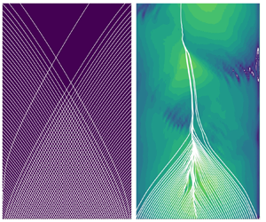
  $z=-1$ are the non-dimensional heights of the top and bottom walls, respectively. Figure 3 shows a single snapshot at time $t=110$ of $u$ (colours) and $\rho$ (contours) at the $y=0$ midplane for the four datasets, highlighting the $\rho =0$ density interface with a thick green contour.

Figure 2. A schematic of two-layer shallow-water flow.

Figure 3. Snapshots at  $t=110$ of streamwise velocity $u$ (blue to red shading) and density $\rho$ (contours) in the midplane ( $y=0$) for the (a) laminar, (b) stationary wave, (c) travelling wave and (d) intermittent cases. The interface $\rho =0$ is emphasised by the thick green line. In (b,c), the interface shows evidence of a jump, with the lower layer travelling from left to right increasing in thickness near $x=0$, and the converse for the upper layer.
3.2. Layer-averaged DNS data and evidence of jumps
Figure 4 illustrates the results obtained after applying this layer averaging to the DNS database. We show  $x$–
$x$– $t$ diagrams of the lower-layer height $h_2$ (figures 4a–d) and lower-layer velocity $u_2>0$ (figures 4e–h) for the laminar (L), stationary wave (SW), travelling wave (TW) and intermittently turbulent (I) cases. The layer averaging (in $y,z$) was performed in the range $|x|\leq 32$, which includes the duct $|x|\le 30$ and extends slightly into the reservoirs where the layers flow in and out.

Figure 4. Spatio-temporal diagrams of (a–d) the lower-layer height  $h_2$ and (e–h) lower-layer velocity $u_2$ from the DNS data for the four flow regimes: (a,e) L, (b, f) SW, (c,g) TW and (d,h) I. All data are for $t\in [80,260]$.
The L flow regime exhibits sudden changes in depth and speed only at the ends of the duct  $x=\pm 30$, as is expected from the flow exiting into the deep reservoirs. Figure 4(a) and an instantaneous snapshot of the flow in figure 3(a) confirm that the interface $\eta (x)$ is steady and gently sloping down ( $\eta '<0$) throughout the duct, and is symmetric with respect to the centre of the duct ( $x=0$), i.e. $\eta (x,t)=\eta (x)=-\eta (-x)$.
In contrast, for the SW and TW flow regimes, a sudden change of contours is observed at  $x\approx 0$, indicating the appearance of an internal hydraulic jump. The lower-layer thickness $h_2$ increases suddenly along the direction of the flow (purple for $x<0$ to orange for $x>0$ in figure 4), which is accompanied by a sudden drop in $u_2$ (dark to light red). This discontinuity indicates the presence of what is commonly called an ‘internal hydraulic jump’ (Baines Reference Baines2016; Thorpe et al. Reference Thorpe, Malarkey, Voet, Alford, Girton and Carter2018), as can be seen in figures 3(b,c), where both layers experience an expansion and deceleration in their respective flow directions. In the SW and TW flows (figures 3b,c), the interface is sloping up ( $\eta '>0$) in the vicinity of the jump, and is negative ( $\eta <0$) throughout most of the left-hand side of the duct, and vice versa, (figure 3a).
Figure 5 shows the temporal evolution of the interface in all four flows, with  $\eta (x,t)$ plotted at intervals separated by one time unit and vertically stacked. In the SW case, the jump remains in the narrow interval $x=\pm 1$, whereas in the TW case, it oscillates over a much larger interval and sends off waves in either direction, hence the distinction between the ‘stationary’ and ‘travelling’ wave regimes. In the I case, moving jumps are observed in the quiet phase ( $150 \lesssim t \lesssim 200$), being initiated near both ends of the duct at $t\approx 150$ and progressively moving towards the centre of the duct. These jumps merge at around $t=200$ and then stay at the middle of the duct $x=0$ for a time ${\approx }20$ before the transition to turbulence occurs at $t \approx 220$ (the active stage of the intermittent cycle).

Figure 5. Temporal evolution of the density interface  $\eta (x,t)$ in (a) L, (b) SW, (c) TW and (d) I. The interface curves are stacked in time at intervals of one time unit. Jumps are revealed in (b–d) by discontinuities in $\eta (x)$.
3.3. Flow rate and evidence of maximal exchange
To a good approximation, the flow in the SID has zero net (barotropic) volume flow rate
 \begin{equation} \langle u \rangle_{y,z} \equiv \frac{1}{4} \int_{{-}1}^{1} \int_{{-}1}^{1} u \, {{\rm d}y} \,{\rm d} z = \frac{1}{2}\,(u_1 h_1 + u_2 h_2) \approx 0, \end{equation}
but a non-zero baroclinic exchange volume flow rate (or volume flux)  $Q(x,t)$ and mass flow rate (or mass flux) $Q_m(x,t)$ defined as
 $$\begin{gather} Q \equiv \langle |u| \rangle_{y,z} = \tfrac{1}{2}(u_2h_2 - u_1h_1) \approx{-}u_1 h_1 \approx u_2 h_2 \quad \text{using}\ (3.3), \end{gather}$$
 $$\begin{gather}Q_m \equiv \langle \rho u \rangle_{y,z} \approx \rho_1 u_1 h_1 \approx \rho_2 u_2 h_2. \end{gather}$$
The approximation in (3.5) comes from the fact that the layer average of the product  $\rho u$ is not exactly equal to the product $\rho _i u _i$ of the layer averages. Also, recall that the non-dimensional density is defined such that the mean density is 0 and the minimum and maximum are $-1$ and 1, respectively.
Hydraulic jumps in two-layer exchange flows are often connected to the notion of maximal exchange, i.e. of an upper bound in the exchange volume flux  $Q$ and mass flux $Q_m$. This means that flows lacking such jumps have a lower $Q$, and that no realisable flow may have a higher $Q$. While hydraulic jumps have not yet been investigated in detail in the experimental SID literature, the mass flux $Q_m$ has, due to the simplicity with which it can be measured.
In figure 6, we show the dependence of the volume flux  $Q$ and the mass flux $Q_m$ on $Ri\,Re \sin \theta \approx (1/4) \theta \,Re$ using its temporal mean (symbols) and extreme values (error bars) in 15 different DNS from Zhu et al. (Reference Zhu, Atoufi, Lefauve, Taylor, Kerswell, Dalziel, Lawrence and Linden2023), containing the four main datasets L, SW, TW and I, as well as 11 others, including one turbulent dataset (T). We find that both $Q$ and $Q_m$ increase approximately linearly with $\theta \,Re$ in the L regime (where little mixing ensures that $Q\approx Q_m$), in agreement with the laminar analytical solution of Duran Matute et al. (Reference Duran Matute, Kaptein and Clercx2023) (the ‘viscous–advection–diffusion’ balance). For higher values of $\theta \,Re$, both $Q$ and $Q_m$ reach an upper bound $\approx 0.5$ in the W regime (SW, TW), and the volume flux $Q$ maintains this value into the I and T regimes, while $Q_m$ drops below $0.5$ in these latter I and T regimes. These observations are consistent with the corresponding experimental data of Lefauve & Linden (Reference Lefauve and Linden2020) (their figures 5 and 6) if we exclude their data at small angles $\theta <2^\circ$ (which behave slightly differently, and we did not simulate them). This apparent upper bound on $Q$ is evidence of maximal exchange since a further increase in $\theta \,Re$ does not lead to an increase in the velocity difference between the upper and lower layers. As will be shown later (§ 5.3), $Q \approx 0.5$ is the threshold of the long-wave instabilities and onset of hydraulic transitions, and a further increase in $Q$ beyond this limit is taxed by turbulent dissipation. The reduction in $Q_m$ below 0.5 at high $\theta \,Re$ is caused by mixing across the shear layer in the I and T regimes, reducing the net mass transport.

Figure 6. (a) The volume flux  $Q$ and (b) the mass flux $Q_m$, from the 15 DNS of Zhu et al. (Reference Zhu, Atoufi, Lefauve, Taylor, Kerswell, Dalziel, Lawrence and Linden2023) plotted against $Ri\,Re \sin \theta$. The symbols, coded by the respective regimes, show the time-averaged value, while the error bars depict the extreme values. While $Q$ asymptotes to ${\approx }0.5$ (maximal exchange), $Q_m$ decreases at high $Re\,{Ri} \sin {\theta }$ because of mixing.
This large body of experimental and numerical evidence in favour of maximal exchange in the SID, and the observation that  $Q, Q_m\approx 0.5$ in the SW and TW regimes, combined with our observations in § 3.2 of the existence of an internal jump, are strongly suggestive that hydraulic effects dominate the flow from the W regime onwards.
In the next section, we develop the two-layer hydraulics framework to study these jumps and maximal exchange, and their relation to the transition from laminar flow to waves and to turbulence in the SID.
4. Two-layer equations: characteristics and instabilities
In this section, we aim to define and relate the characteristic velocity of the two-layer flows in the context of the SID to the hydraulic regime of the flow. We also aim to provide a physical implication of when this characteristic velocity is not purely real. We start by simplifying the inviscid Navier–Stokes equations using the shallow-water (long-wave) approximation in §§ 4.1–4.3, before comparing it to the Taylor–Goldstein (linear wave) theory in §§ 4.4 and 4.5, and interpreting our findings in § 4.6.
4.1. Shallow-water equations: nonlinear hydrostatic waves
The shallow-water approximation that assumes the pressure is hydrostatic is verified in Appendix A. Under this approximation the upper layer obeys
 \begin{equation} \left.\begin{gathered}
\frac{{\partial} h_1}{{\partial} t} + \frac{{\partial} (h_1
{u}_1)}{{\partial} x}=0,\\ \begin{aligned}&\frac{{\partial} (h_1
{u}_1)}{{\partial} t} + \frac{{\partial} }{{\partial}
x}\left(h_1{u}_1^2+ Ri
\cos{\theta}\,{\rho}_1\,\frac{h_1^2}{2}\right)\\
&\quad =Ri
\sin{\theta}\,{\rho}_1 h_1 -Ri
\cos{\theta}\,h_1\,\frac{{\partial}}{{\partial} x}
(p_w+{\rho}_1 h_2+{\rho}_1 b ), \end{aligned}
\end{gathered}\right\}
\end{equation}
\begin{equation} \left.\begin{gathered}
\frac{{\partial} h_1}{{\partial} t} + \frac{{\partial} (h_1
{u}_1)}{{\partial} x}=0,\\ \begin{aligned}&\frac{{\partial} (h_1
{u}_1)}{{\partial} t} + \frac{{\partial} }{{\partial}
x}\left(h_1{u}_1^2+ Ri
\cos{\theta}\,{\rho}_1\,\frac{h_1^2}{2}\right)\\
&\quad =Ri
\sin{\theta}\,{\rho}_1 h_1 -Ri
\cos{\theta}\,h_1\,\frac{{\partial}}{{\partial} x}
(p_w+{\rho}_1 h_2+{\rho}_1 b ), \end{aligned}
\end{gathered}\right\}
\end{equation}and the lower layer obeys
 \begin{equation} \left.\begin{gathered}
\frac{{\partial} h_2}{{\partial} t} + \frac{{\partial} (h_2
{u}_2)}{{\partial} x}=0,\\ \begin{aligned} &\frac{{\partial} (h_2
{u}_2)}{{\partial} t} + \frac{{\partial} }{{\partial}
x}\left(h_2{u}_2^2+ Ri
\cos{\theta}\,{\rho}_2\,\frac{h_2^2}{2}\right)\\
&\quad =Ri \sin{\theta}\,{\rho}_2 h_2
-Ri\cos{\theta}\,h_2\, \frac{{\partial}}{{\partial} x}
(p_w+{\rho}_1 h_1+ {\rho}_2 b ). \end{aligned}
\end{gathered}\right\}
\end{equation}
\begin{equation} \left.\begin{gathered}
\frac{{\partial} h_2}{{\partial} t} + \frac{{\partial} (h_2
{u}_2)}{{\partial} x}=0,\\ \begin{aligned} &\frac{{\partial} (h_2
{u}_2)}{{\partial} t} + \frac{{\partial} }{{\partial}
x}\left(h_2{u}_2^2+ Ri
\cos{\theta}\,{\rho}_2\,\frac{h_2^2}{2}\right)\\
&\quad =Ri \sin{\theta}\,{\rho}_2 h_2
-Ri\cos{\theta}\,h_2\, \frac{{\partial}}{{\partial} x}
(p_w+{\rho}_1 h_1+ {\rho}_2 b ). \end{aligned}
\end{gathered}\right\}
\end{equation}
Here,  $p_w(x,t)$ is the pressure at the upper wall, and $b(x)$ is the elevation of the bottom wall relative to $z=0$. Conveniently, the bottom wall in the SID is fixed at $b(x)=-1$. We subtract the momentum equations in (4.1) from (4.2) to remove $p_w$ and reduce the number of unknowns. The streamwise variation of density of the upper and lower layers is also neglected compared to variations in the height of the layers (i.e. $\partial (\rho h)/\partial x \approx \rho \,\partial h/\partial x$). The shallow-water equations (SWEs) become
 \begin{align} &\frac{{\partial} h_2}{{\partial} t} -\frac{{\partial} h_1}{{\partial} t} + h_2\,\frac{{\partial} u_2}{{\partial} x}- h_1\, \frac{{\partial} u_1}{{\partial} x}+u_2\,\frac{{\partial} h_2}{{\partial} x} -u_1\,\frac{{\partial} h_1}{{\partial} x}=0, \end{align}
 \begin{align} & \frac{{\partial} u_2}{{\partial} t} -\frac{{\partial} u_1}{{\partial} t} + u_2\,\frac{{\partial} u_2}{{\partial} x}-u_1\, \frac{{\partial} u_1}{{\partial} x} +Ri \cos{\theta}\,(\rho_2-\rho_1)\,\frac{{\partial} h_2}{{\partial} x} \nonumber\\ &\quad =Ri \sin{\theta}\,(\rho_2-\rho_1) -Ri \cos{\theta}\,(\rho_2-\rho_1)\,\frac{{\partial} b}{{\partial} x}, \end{align}
with two auxiliary equations to satisfy the no net (barotropic) flow condition and geometric constraint inside the duct  $({{\partial } b}/{{\partial } x}=0)$:
 \begin{equation} u_1 h_1 + u_2 h_2 = 0, \quad h_1 + h_2 = 2. \end{equation}
By taking the derivative of (4.5a,b) with respect to  $x$, these four equations can be written compactly as
 \begin{equation} {{\boldsymbol{\mathsf{C}}}}\,\frac{{\partial} \boldsymbol{q}}{{\partial} t}+ {{\boldsymbol{\mathsf{A}}}}(\boldsymbol{q},{\rm \Delta} \rho)\, \frac{{\partial} \boldsymbol{q}}{{\partial} x}=\boldsymbol{f}, \end{equation}
where the state vector  $\boldsymbol {q}$ and coefficient matrices ${{\boldsymbol{\mathsf{A}}}}, {{\boldsymbol{\mathsf{C}}}}$ are
 \begin{equation} \left.\begin{gathered} \boldsymbol{q}=\left[\begin{array}{c} u_1 \\ u_2 \\ h_1 \\ h_2 \end{array}\right],\quad {{\boldsymbol{\mathsf{A}}}}=\left(\begin{array}{cccc} -u_1 & u_2 & 0 & Ri\cos\theta\,{\rm \Delta}\rho \\ -h_1 & h_2 & -u_1 & u_2 \\ 0 & 0 & 1 & 1\\ h_1 & h_2 & u_1 & u_2 \end{array}\right),\\ {{\boldsymbol{\mathsf{C}}}}=\left(\begin{array}{cccc} -1 & 1 & 0 & 0 \\ 0 & 0 & -1 & 1 \\ 0 & 0 & 0 & 0\\ 0 & 0 & 0 & 0 \end{array}\right). \end{gathered}\right\} \end{equation}
The SWE (4.6) are quasi-linear, i.e. linear in the derivatives of  $\boldsymbol {q}$ but with the coefficient matrix ${{\boldsymbol{\mathsf{A}}}}$ dependent on $\boldsymbol {q}$. The quasi-constant local density difference between layers is defined as ${\rm \Delta} \rho (x,t) \equiv \rho _2-\rho _1\in (0,2)$ (specified by our layer-averaged DNS data). This equation does not assume that interfacial waves have infinitesimal amplitudes, but it does assume, through the hydrostatic assumption, that waves are long with respect to the layer height (i.e. that their non-dimensional wavenumber satisfies $k\ll 1$). In the following, we neglect the forcing
 \begin{equation} \boldsymbol{f}=[Ri\sin\theta\,{\rm \Delta}\rho, 0, 0, 0]^{\rm T}, \end{equation}
recalling that  $\sin \theta \ll 1$. We will study (4.6) in the homogeneous limit ( $\boldsymbol {f}=\boldsymbol {0}$). We are particularly interested in the eigenvalues of ${{\boldsymbol{\mathsf{A}}}}$, in which $\boldsymbol {f}$ plays no role. The role of forcing, which provides a source term along the characteristics, in shallow-water theory is an interesting question left for future work.
4.2. Characteristic curves and propagation of information
Consider a left eigenvector  $\boldsymbol {v}$ and eigenvalue $\lambda$ associated with the matrix pair $({{\boldsymbol{\mathsf{A}}}},{{\boldsymbol{\mathsf{C}}}})$ such that $\boldsymbol {v}^H {{\boldsymbol{\mathsf{A}}}} = \lambda \boldsymbol {v}^H {{\boldsymbol{\mathsf{C}}}}$, where superscript $H$ denotes Hermitian transpose. Multiplying (4.6) by $\boldsymbol {v}^H$ yields
 \begin{equation} \boldsymbol{v}^H {{\boldsymbol{\mathsf{C}}}} \left(\frac{{\partial} \boldsymbol{q}}{{\partial} t}+\lambda(x,t)\, \frac{{\partial} \boldsymbol{q}}{{\partial} x}\right)=\boldsymbol{0}. \end{equation}
The eigenvalues  $\lambda$ are called characteristic velocities, since they define characteristic curves $s$ in the $(x,t)$ plane along which the partial differential equation (4.6) reduces to an ordinary differential equation (Whitham Reference Whitham2011). For this homogeneous equation, the combination of flow variables $\boldsymbol {v}^H{{\boldsymbol{\mathsf{C}}}} \,\textrm {d}\boldsymbol {q}/\textrm {d} s = \boldsymbol {0}$ is conserved. These characteristic velocities, henceforth referred to simply as ‘characteristics’, can be complex, $\lambda =\lambda ^R + \textrm {i}\lambda ^I \in \mathbb {C}$. Their real part $\lambda ^R \equiv \mbox {Re}{(\lambda )}$ represents the phase speed of shallow-water waves, describing the trajectories $s$. Their imaginary part $\lambda ^I \equiv \mbox {Im}{(\lambda )}$ represents any potential growth ( $\lambda ^I>0$) or decay ( $\lambda ^I<0$) of these waves. The direction of information propagation is set by the sign of $\lambda ^R$: when $\lambda ^R>0$, information propagates rightwards (towards increasing $x$), and vice versa, whereas $\lambda ^R=0$ indicates stationary waves.
The characteristics  $\lambda$ are given by the two distinct solutions of $\det ({{\boldsymbol{\mathsf{A}}}}-\lambda {{\boldsymbol{\mathsf{C}}}})=0$:
 \begin{align} \lambda_{1,2}(x,t) &=
\underbrace{\frac{h_1 u_2 +h_2 u_1 }{h_1 +h_2
}}_{{convective\ velocity}\ \equiv \bar{\lambda}}\ \pm\ \underbrace{\sqrt{\frac{{\rm \Delta}\rho\,Ri \cos{\theta}\,h_1
h_2}{h_1 +h_2}\, {(1-F_{\varDelta}^2 )}}}_{{phase\ speed}\
\equiv\ \delta \lambda} \end{align}
\begin{align} \lambda_{1,2}(x,t) &=
\underbrace{\frac{h_1 u_2 +h_2 u_1 }{h_1 +h_2
}}_{{convective\ velocity}\ \equiv \bar{\lambda}}\ \pm\ \underbrace{\sqrt{\frac{{\rm \Delta}\rho\,Ri \cos{\theta}\,h_1
h_2}{h_1 +h_2}\, {(1-F_{\varDelta}^2 )}}}_{{phase\ speed}\
\equiv\ \delta \lambda} \end{align}
 \begin{align} &\approx \qquad\overbrace{\frac{-2\eta Q}{1-\eta^2}} \quad\ \ \pm \quad\ \ \overbrace{\sqrt{\frac{{\rm \Delta}\rho}{2}\cos\theta\,(1-\eta^2)(1-F_\varDelta^2)}} \quad \text{using}\ (3.4), \end{align}
where
 \begin{align} F_{\varDelta}^2(x,t)&=\frac{({u}_2-{u}_1)^2}{{\rm \Delta}\rho\,Ri \cos{\theta}\,(h_1 +h_2)} \end{align}
 \begin{align} &\approx \frac{2}{{\rm \Delta}\rho \cos \theta}\left(\frac{2Q}{1-\eta^2}\right)^2 \quad \text{using}\ (3.4). \end{align}
 Here, (4.11) and (4.13) use the volume flux  $Q>0$ in (3.4) (which is an approximation relying on (3.3)) and the interface position instead of the layer heights and velocities, as well as the fact that $Ri=1/4$ and $h_1+h_2=2$ in the SID. We see that the characteristics consist of a convective velocity $\bar {\lambda }$ and a phase speed $\delta \lambda$, which can be imaginary, depending on the value of the ‘stability Froude number’ $F^2_{\varDelta }$ (Long Reference Long1956; Lawrence Reference Lawrence1990; Dalziel Reference Dalziel1991). Note that (4.7a–c), (4.10) and (4.12) are slightly modified versions of those given in previous studies (Long Reference Long1956; Armi Reference Armi1986; Lawrence Reference Lawrence1993) adapted to SID flows.
If  $F_{\varDelta }^2<1$, then the two characteristics $\lambda _{1,2}=\bar \lambda \pm \delta \lambda$ are real, and information propagates in both directions relative to the convective velocity $\bar {\lambda }$. The absolute direction of propagation is given by the sign of $\lambda _{1,2}$, to which we will return in § 4.3.
If  $F_{\varDelta }^2>1$, then the characteristics become complex conjugates $\lambda _{1,2} =\lambda ^R\pm \textrm {i}\lambda ^I = \bar {\lambda }$ $\pm \textrm {i}\,|\delta \lambda |$, indicating that the system is no longer hyperbolic and that waves are temporally unstable. The condition $F_{\varDelta }^2>1$ is sometimes known as Long's instability criterion (Long Reference Long1956), although it is quoted in Lamb (Reference Lamb1932) and likely dates back to Helmholtz. The real part is the convective velocity, i.e. information propagates in only one direction, and the growth rate is $\lambda ^I=|\delta \lambda |=\sqrt {({\rm \Delta} \rho /2)\cos \theta \,(1-\eta ^2)(F_\varDelta ^2-1)}$.
Figures 7(a–c) show how  $\lambda _{1,2}$ vary with the volume flux $Q$ and interface position $\eta$ following (4.11), assuming no mixing ( ${\rm \Delta} \rho =2$) and a horizontal duct ( $\cos \theta =1$). We compare the case where the interface is locally symmetric ( $\eta =0$, figure 7b) to the cases where it is asymmetric, i.e. above or below the mid-level ( $\eta =\pm 0.5$ in figures 7(a,c), respectively). Figure 7(b) shows that with a symmetric interface, $\lambda _{1,2}=\pm \sqrt {1-4Q^2}$ are real (red curves) for $Q\le 0.5$, and become purely imaginary (blue curves) for $Q>0.5$. However, when the interface is either below or above the midplane ( $\eta =\pm 0.5$, figures 7a,c), this transition to instability occurs at a lower critical volume flux $Q>Q_c \approx 0.4$. In summary, instability is caused, for a given volume flux $Q$, by an increasingly asymmetric interface $|\eta |$, and vice versa, for a given interface position, by an increasing volume flux $Q$. This offers a possible explanation for the transition from L to W flow observed in figure 6.

Figure 7. Real and imaginary parts of the eigenvalues of the two-layer SWE in (4.11) at (a) positive, (b) zero and (c) negative interface elevations  $\eta$ as functions of the volumetric flow rate $Q$. The eigenvalues are always complex for $Q\ge Q_c=0.5$, and become complex for slightly lower critical values $Q_c\approx 0.4$ in the asymmetric cases (a,c).
4.3. Composite Froude number and hydraulic control
To further stress the importance of the characteristics  $\lambda _{1,2}$, we return to the original SWE (4.6), and note that a non-trivial steady solution $\boldsymbol {q}(x)$ requires $\det {{\boldsymbol{\mathsf{A}}}} \neq 0$, i.e.
 \begin{equation} \det {{\boldsymbol{\mathsf{A}}}}=2\,{\rm \Delta}\rho\,h_1 h_2\, Ri \cos{\theta}\,(G^2-1) \neq 0 \quad \Leftrightarrow \quad G^2 \neq 1, \end{equation}
where  $G^2$ is the squared composite Froude number defined with the Froude numbers of the upper and lower layers, $F_1$ and $F_2$, respectively,
 \begin{equation} G^2=F_1^2+F_2^2,\quad F_i=\frac{{u}_i}{\sqrt{{\rm \Delta}\rho\,Ri \cos{\theta}\,h_i}}, \quad i=1,2. \end{equation}
Points at which  $G^2=1$ are called control points (Armi Reference Armi1986; Lawrence Reference Lawrence1990; Dalziel Reference Dalziel1991). At control points, ${{\boldsymbol{\mathsf{A}}}}$ is non-invertible, and a regularity condition must exist to recover a steady solution.
The link between characteristics and the composite Froude number can be highlighted with the identity
 \begin{align}
G^2=1+\frac{h_1+h_2}{\Delta \rho\,Ri
\cos{\theta}\,h_1 h_2}\, \lambda_1 \lambda_2 &=
1+\frac{2\lambda_1\lambda_2}{{\rm \Delta}\rho\cos\theta\,(1-\eta^2)}
,
\end{align}
\begin{align}
G^2=1+\frac{h_1+h_2}{\Delta \rho\,Ri
\cos{\theta}\,h_1 h_2}\, \lambda_1 \lambda_2 &=
1+\frac{2\lambda_1\lambda_2}{{\rm \Delta}\rho\cos\theta\,(1-\eta^2)}
,
\end{align} \begin{align} &\approx 1+\sqrt{\frac{2}{{\rm \Delta}\rho \cos\theta}}\, \frac{\lambda_1\lambda_2F_\varDelta}{2Q}, \quad \text{using}\ (4.13). \end{align}
From this expression, we deduce the following, illustrated in figure 8.


If the waves are stable ( $F_\varDelta ^2<1$), then the characteristics $\lambda _{1,2}$ are real. The flow is called subcritical, and information propagates in both directions (along positive and negative $x$), i.e. $\lambda _1\lambda _2<0 \Leftrightarrow G^2<1$. In other words, the absolute phase speed $|\delta \lambda |$ is larger than the absolute convective velocity $\bar {\lambda }$ in (4.10). Vice versa, the flow is called supercritical when information propagates in only one direction, i.e. $\lambda _1\lambda _2>0 \Leftrightarrow G^2>1$, and the absolute phase speed $|\delta \lambda |$ is smaller than the absolute convective velocity $\bar {\lambda }$. Note that for supercritical flow, the direction of propagation associated with $\lambda _1$ and $\lambda _2$ is the same as that given by the convective velocity $\bar \lambda$, i.e. the waves are swept downstream.
If, on the other hand, the waves are unstable ( $F_\varDelta ^2>1$), then the characteristics are complex conjugates $\lambda _{1,2}=\lambda ^R \pm \textrm {i}\lambda ^I$, i.e. information always propagates in a single direction given by the sign of $\lambda ^R=\bar \lambda$, and the flow is always supercritical ( ${\lambda _1 \lambda _2=(\lambda ^R)^2+(\lambda ^I)^2>0 \Leftrightarrow G^2>1}$). Under unstable conditions, control points where $G^2=1$ cannot exist, but points can exist where stationary ( $\lambda ^R=0$) waves grow ( $\lambda ^I>0$) and control the flow.
In summary, the SWE predicts that information propagates along a pair of trajectories  $\lambda _{1,2}$ that arise from the solution of a generalised eigenvalue problem and depend on the local ( $x$) and instantaneous ( $t$) state of the two-layer representation. The solutions $\lambda _{1,2}=\bar \lambda \pm \delta \lambda$ have a real convective velocity $\bar \lambda$ and a phase speed $\delta \lambda$, which may be either real or imaginary. When $\lambda _{1,2}$ are real ( $\delta \lambda \in \mathbb {R}$), they represent the propagation of two (neutrally stable) kinematic waves with phase speed $\delta \lambda$ relative to the convective velocity $\bar \lambda$. The respective signs of $\lambda _{1,2}$ determine the direction of information propagation and whether the flow is subcritical (composite Froude number $G^2<1$, product $\lambda _1\lambda _2<0$) with information propagating in both directions, or supercritical ( $G^2>1$, $\lambda _1\lambda _2>0$) with information propagating only in the direction given by the sign of $\bar \lambda$. When $\lambda _{1,2}$ are complex ( $\lambda _{1,2}=\lambda ^R \pm \textrm {i}\lambda ^I=\bar \lambda \pm \textrm {i}\,|\delta \lambda |$), the real part still represents a convective velocity that carries information, while the positive imaginary part indicates that the flow is unstable. Although in this unstable case the SWE is no longer hyperbolic, the flow may be viewed as supercritical ( $G^2>1$) in the sense that information is propagated only in the direction given by $\bar \lambda =\lambda ^R$, and as hydraulically controlled when $\bar \lambda =0$.
In the following subsections, we clarify the interpretation of unstable shallow-water waves using linear stability analysis around a locally parallel base flow. In § 4.4, we take the long-wave limit of solutions of the Taylor–Goldstein equations; in § 4.5, we study the link between long and short waves; and in § 4.6, we linearise the SWEs assuming the waves are sufficiently (but not excessively) long.
4.4. Taylor–Goldstein equations: linear short and long waves
We relax the previous restriction that waves must be long ( $k \ll 1$) by studying waves of possibly larger $k$ but of infinitesimal amplitude developing on a parallel base flow described by a velocity profile $\mathcal {U}(z)$ and a density profile $\mathcal {R}(z)$. The perturbation streamfunction $\hat {\psi }(z) \exp \textrm {i}k(x-ct)$ describing the evolution of these two-dimensional linear waves is given by the inviscid Taylor–Goldstein equation (TGE)
 \begin{equation} (\mathcal{U}-c) \left(\frac{{{\rm d}}^2 }{{{\rm d}} z^2}-k^2\right)\hat{\psi}-\mathcal{U}'' \hat{\psi} - \frac{Ri \cos{\theta}\,\mathcal{R}'}{\mathcal{U}-c}\,\hat{\psi} = 0. \end{equation}
This equation can be analysed following standard methods (e.g. Drazin Reference Drazin2002; Smyth & Carpenter Reference Smyth and Carpenter2019), with details given in Appendix B. Note that we assumed small tilt angles  $0<\sin {\theta } \ll \cos {\theta }$, although the more general TGE in Appendix B shows that $\sin \theta$ has a destabilising effect (ignored here). In the ordinary differential equation above, a prime denotes differentiation with respect to $z$, and $c \in \mathbb {C}$ is the phase speed of the plane waves, akin to the characteristics $\lambda$ of the SWE. However, we use a different notation for the characteristics of shallow-water nonlinear waves and the phase speed of Taylor–Goldstein linear waves to emphasise that while the former implicitly assumes $k\ll 1$, the latter implicitly assumes $k \gg A^{-1}$. In other words, the Taylor–Goldstein linear waves that we investigate should be much shorter than the duct length $A$ for the local analysis on a parallel base flow to be sensible. In other words, $k \gg A^{-1}$ ensures that the waves do not ‘feel’ the streamwise variations of the base flow along the duct.
To establish a link with two-layer characteristics and obtain solutions for  $c$, we assume a two-layer flow bounded by solid boundaries, with fixed layer heights $h_1, h_2$, velocities $u_1,u_2$, and an interface at $z=0$, consistent with the two-layer model adopted throughout this paper:
 \begin{equation} \mathcal{U}(z)= \begin{cases} u_1, & 0 < z \le h_1, \\ u_2, & -h_2 \le z < 0, \end{cases}\quad \mathcal{R}(z)= \begin{cases} \rho_1, & 0 < z \le h_1, \\ \rho_2, & -h_2 \le z < 0. \end{cases} \end{equation}
Note that  $h_1+h_2=2$, and by a simple vertical shift, the above model is equivalent to having a domain restricted to $z=\pm 1$ and an interface at an arbitrary $z=\eta$ (giving $h_{1,2}=1\pm \eta$). In § 5.5, we will use the velocity, height and density of layers from the DNS data to specify $\mathcal {U}$ and $\mathcal {R}$.
By enforcing the matching conditions for the streamfunction and pressure at the interface (see Appendix B), we derive the dispersion relation for the complex phase speeds:
 \begin{equation} \left.\begin{gathered} c_{1,2}=\frac{u_1+u_2}{2} + \frac{ (\sigma_5-\sigma_6) (u_1-u_2) \pm \sigma_2 }{2{(\sigma_1 -1)}}, \\ \sigma_1 =\cosh (4k ),\quad \sigma_2 =\sinh (2k) \varLambda,\quad \sigma_3 =\sinh (2k h_2), \\ \sigma_4 =\sinh (2k h_1),\quad \sigma_5 =\cosh (2 kh_2),\quad \sigma_6 =\cosh (2 k h_1 ), \\ \varLambda =\sqrt{-\frac{4}{k} \left(k\sigma_4 \sigma_3 [ {u_1 }-{u_2 }]^2 + Ri \cos{\theta}\,[\sigma_4(1-\sigma_5)+\sigma_3(1-\sigma_6)]\,{\rm \Delta}\rho \right)}. \end{gathered}\right\} \end{equation}
These waves are the well-known Kelvin–Helmholtz (KH) waves supported by a single vortex sheet (see e.g. § 4.6.1 of Smyth & Carpenter Reference Smyth and Carpenter2019). They are modulated by stratification; increasing  $Ri \cos \theta \,{\rm \Delta} \rho$ always stabilises them. Importantly, the dispersion relation (4.20) describes waves in a domain bounded by the top and bottom boundaries, which, as we will see, strongly affect waves that have a wavelength comparable to or longer than the domain height.
For ‘short’ waves – i.e. having a wavelength of the order of the duct height  $k=O(1)$ or shorter, $k>1$ – the dispersion relation (4.20) cannot be simplified further, and these waves are dispersive. These will be referred to simply as KH waves, as in the short-wave limit they are identical to those found in vertically unbounded domains.
For ‘long’ waves (which, for clarity, we do not call KH waves) – i.e. having a wavelength much longer than the duct height, but still shorter than the duct length,  $A^{-1} \ll k \ll 1$ – the dispersion relation (4.20) simplifies as $\sinh {k h} \rightarrow k h$ and $\cosh {k h} \rightarrow 1$, and (4.20) reduces to (4.10), i.e.
 \begin{equation} c_{1,2} (k) \rightarrow \lambda_{1,2} \quad \text{when}\ k\ll 1, \end{equation}
and these waves are non-dispersive. In other words, the characteristics  $\lambda _{1,2}$ of nonlinear shallow-water waves can be identified with the phase speeds $c_{1,2}$ of linear (infinitesimal) long waves calculated assuming the local two-layer flow $(u_1,u_2,h_1,h_2)$ to be parallel and steady as in (4.19a,b).
The dispersion relation (4.20) shows that there exists a smooth transition between short KH waves and long shallow-water waves, as those waves differ by their wavelength but not the underlying physical mechanism.
Although the limit (4.21) can be inferred from Gu (Reference Gu2001) (§ 3.3) and is alluded to briefly in Boonkasame & Milewski (Reference Boonkasame and Milewski2012) (§ 3), it does not appear to be disseminated widely in the hydraulics literature. We visualise this smooth transition next.
4.5. Long versus short waves
Figure 9 shows the dispersion relation from the TGE (4.20) with the phase speed  $\mbox {Re}(c_1) = c_1^R$ (blue to red contours) and growth rate $\mbox {Im}(c_1) = c_1^I$ (colour map with deep blue being stable) as functions of the wavenumber $k$ (vertical axis) and the volume flux $Q$ (horizontal axis). We compare a symmetric interface ( $\eta =0$, figure 9a), an asymmetric interface ( $\eta =-0.5$, figure 9b), and a case with a symmetric interface but without solid top and bottom boundaries (figure 9c), whose dispersion relation (B13) is derived analytically in § B.3.

Figure 9. Dispersion relation of all (long and short) inviscid two-layer waves: growth rate (colours) and phase speed (contours) solutions of the TGE varying with wavenumber  $k$ and volume flux $Q$. (a) Symmetric interface $\eta =0$. (b) Asymmetric interface $\eta =-0.5$. (c) Symmetric interface but without solid top and bottom boundaries at $z=\pm 1$, in which case the long waves of the SWE disappear.
First, figures 9(a,b) show that long waves are non-dispersive (the phase speed contours do not depend on  $k$). Second, long waves become unstable (lighter shades of blue and green) above a critical volume flux $Q> Q_c$, equal to $0.5$ for a symmetric interface (figure 9a) and lower than $0.5$ for an asymmetric interface (figure 9b). Third, for a symmetric interface, all unstable waves (long and short) are stationary (absence of contours), but all stable waves are travelling (presence of contours). For an asymmetric interface, even unstable waves travel in the reference frame of the duct. Fourth, the transition between short and long waves is smooth, i.e. there is a continuity between the long shallow-water waves controlling the hydraulics of two-layer flows and the short KH waves.
Figures 9(a,b) also provide further insights. First, short waves ( $k \not \ll 1$) become unstable at smaller values of $Q$ compared to the long-wave threshold $Q_c$. This transition to short waves becomes noticeable from $k\gtrsim 10^{-0.5}\approx 0.3$, and is clear for $k>1$. The shortest waves shown here ( $k=10^2$) are predicted to become unstable above a very small volume flux $Q\gtrsim 0.1$. However, we note that this threshold would be closer to the long-wave $Q_c$ if we included viscosity in the TGE, as viscosity would significantly dampen the growth of short waves. These plots show that for a given value of $Q$, the growth rate increases monotonically with $k$ (i.e. the shortest waves are the most unstable). As is often the case, this ‘ultraviolet catastrophe’ would be regularised by viscosity, with the probable existence of a maximum growth rate at an intermediate $k$ for intermediate values of $Re$.
$Re$.
Figure 9(c) shows that the absence of top and bottom boundaries does not affect short waves (the colours and contours at  $k\gtrsim 3$ are identical to figure 9a), because they do not ‘feel’ the presence of the boundaries. However, the absence of solid boundaries precludes the existence of unstable long waves, $k\lesssim 0.3$, and all unstable linear waves are ‘short’ and dispersive. In other words, this analysis shows explicitly that the presence of solid boundaries in the SID is crucial to explain the leading-order dynamics in the DNS by allowing long-wave instability. In short, adding boundaries (figure 9a) creates the long waves on which hydraulic effects rely, and long waves transition smoothly into short waves as $k$ increases.
In Appendix C, we study how the growth of long waves is impacted by smooth, diffuse (i.e. not strictly two-layer) density and velocity profiles, which are expected in all real-world flows (having finite  $Re$ and $Pr$). We show that long waves become unstable when $Q>Q_c$ even for different smoothed profiles such as hyperbolic tangent or sinusoidal mean profiles.
4.6. Link between complex characteristics and instability
The natural link between  $\lambda _{1,2}$ and $c_{1,2}$ in the long-wave limit (4.21) can be understood further by considering another limit. It is possible to linearise directly the SWE (4.6) to study the evolution of infinitesimal perturbations $\epsilon \,\tilde {\boldsymbol {q}}(x,t)$ ( $0<\epsilon \ll 1$) on a parallel, steady base flow $\boldsymbol {q}_0=(u_1,u_2,h_1,h_2)$ akin to (4.19a,b). We perform a first-order Taylor expansion of the coefficient matrix from (4.7a–c), ${{\boldsymbol{\mathsf{A}}}}(\boldsymbol {q}) = {{\boldsymbol{\mathsf{A}}}}(\boldsymbol {q}_0+\epsilon \tilde {\boldsymbol {q}})$, and obtain
 \begin{equation} {{\boldsymbol{\mathsf{C}}}}\,\frac{{\partial} (\boldsymbol{q}_0+\epsilon\tilde{\boldsymbol{q}})}{{\partial} t}+ \left[{{\boldsymbol{\mathsf{A}}}}(\boldsymbol{q}_0)+\epsilon \tilde{\boldsymbol{q}}\, \frac{\partial {{\boldsymbol{\mathsf{A}}}}}{\partial \boldsymbol{q}_0}\right] \left[\frac{{\partial} \boldsymbol{q}_0}{{\partial} x} +\epsilon\,\frac{{\partial} \tilde{\boldsymbol{q}}}{{\partial} x}\right]=0. \end{equation}
At order  $\epsilon$, we have the linear, local SWE
 \begin{equation} {{\boldsymbol{\mathsf{C}}}}\,\frac{{\partial} \tilde{\boldsymbol{q}}}{{\partial} t}+ {{\boldsymbol{\mathsf{A}}}}_0\, \frac{{\partial} \tilde{\boldsymbol{q}}}{{\partial} x}={-}\tilde{\boldsymbol{q}}\, \frac{{\partial} {{\boldsymbol{\mathsf{A}}}}}{{\partial} \boldsymbol{q}_0} \underbrace{\frac{{\partial} \boldsymbol{q}_0}{{\partial} x}}_{{=}0}, \end{equation}
where  ${{\boldsymbol{\mathsf{A}}}}_0\equiv {{\boldsymbol{\mathsf{A}}}}(\boldsymbol {q}_0)$ is the local constant-coefficient matrix. Importantly, the right-hand side coming from the Taylor expansion, and acting as a forcing term, vanishes when we assume that the base flow varies slowly. Substituting the plane wave ansatz $\tilde {\boldsymbol {q}} = \hat {\boldsymbol {q}}\exp {\textrm {i}k(x-\varsigma t)}$ gives the phase speed $\varsigma$ as the eigenvalue of the matrix pair $({{\boldsymbol{\mathsf{A}}}}_0,{{\boldsymbol{\mathsf{C}}}})$. The two distinct solutions $\varsigma _{1,2}$ of $\det ({{\boldsymbol{\mathsf{A}}}}_0-\varsigma {{\boldsymbol{\mathsf{C}}}})=0$ then become identical to the local characteristics $\lambda _{1,2}$ (at fixed $x,t$) derived in (4.10).
In other words, the nonlinear shallow-water wave ( $k\ll 1$) characteristics $\lambda _{1,2}$ can be interpreted as the linear shallow-water waves phase speed $\varsigma _{1,2}$ propagating on a locally parallel base flow ( $k\gg A^{-1}$), which are themselves the long-wave, non-dispersive limit case of the Taylor–Goldstein two-layer phase speeds $c_{1,2}$. Ultimately, this result stems from the fact that, simply put, the linearisation and the long-wave limit commute. In particular, the potential positive imaginary component of characteristics $\lambda ^I>0$ can be interpreted as the exponential growth rate of such unstable waves satisfying $A^{-1} \ll k \ll 1$.
This interpretation is summarised in figure 10. The long aspect ratio  $A$ of the SID (in this paper, $A=30$), ensures that the range of waves $A^{-1} \ll k \ll 1$ exists, and therefore that this interpretation is useful, unlike in shorter geometries having $A\lesssim 10$. However, we note that this interpretation becomes questionable near the duct inlet and outlet if the base flow variations in $x$ are significant. We also note that this interpretation can be generalised to any number of layers greater than two.

Figure 10. (a) Summary of the interpretation of characteristics in § 4.2 using linear theory, either by first linearising the Navier–Stokes equations, and then taking the long-wave limit (TGE, § 4.4), or vice versa (SWE, § 4.6). Both approaches yield the same result for waves much shorter than the duct length but much longer than the duct height (range sketched in (b)).
5. Two-layer hydraulics applied to DNS
In this section, we use the modelling results of § 4 to understand the observations of hydraulic jumps and maximal exchange of § 3. In § 5.1, we study the stability Froude number flagging long-wave instability; in § 5.2, we focus on the characteristics and composite Froude number to diagnose internal jumps and hydraulic control; and in § 5.3, we explain the observed flow rate with notions of maximal exchange, viscous friction and mixing.
5.1. Stability Froude number and instability
In figure 11, we plot the spatio-temporal diagram of the stability Froude number  $F_\varDelta ^2(x,t)$ given by (4.12) in our four datasets L, SW, TW and I (all at $Re=650$) to diagnose any long-wave instability.

Figure 11. Spatio-temporal diagram ( $x-t$) of the stability Froude number $F_\varDelta ^2$ for the (a) L, (b) SW, (c) TW and (d) I cases. Long-wave instability is predicted for $F_\varDelta ^2>1$ (red). The dashed lines represent $t=110$ (L, SW and TW) and $t=180$ (I) when snapshots in figure 3 were plotted.
The laminar flow (L) has  $F_\varDelta ^2<1$ everywhere (in blue in figure 11a), hence long waves are stable at $\theta =2^\circ$. In all other cases, $F_\varDelta ^2>1$ (in red in figure 11) in most of the duct, hence long waves are unstable at $Re=650$ for $\theta > \theta _c$, where $\theta _c\in [2^\circ, 5^\circ ]$. In the wave flows (SW and TW), the waves are most unstable (maximum $F_\varDelta ^2$, deep red) near the centre of the duct. In the I flow, long waves are very unstable ( $F_\varDelta ^2\gg 1$) throughout most of the duct. These diagrams also show that as the tilt angle $\theta$ is increased modestly between $5^\circ$ (figure 11c), and $8^\circ$ (figure 11d), further changes take place as the flow becomes increasingly unstable to long waves. Next, we delve deeper into the hydraulics analysis to understand jumps by focusing on the characteristics in each flow.
5.2. Characteristics, composite Froude number and control
In figure 12, we plot the characteristic velocities  $\lambda _{1,2}(x)$ given by (4.10) (real parts in figure 12a and imaginary parts in figure 12b), and the composite Froude number $G^2(x)$ given by (4.17) (figure 12c) at time $t=110$, to diagnose the propagation of information and criticality of the flow, respectively. In figure 13, we plot a set of discrete trajectories (white curves) by solving
 \begin{equation} \frac{{\rm d} X}{{\rm d} t} = \lambda^R(X,t) \quad \text{for}\ t>80, \end{equation}
and initialising  $X(t=80)$ as 61 equidistant points along the duct $x\in [-30,30]$. Additionally, we plot the local growth rate $\lambda ^I(x,t)$ in background colours (dark blue to yellow) for comparison.

Figure 12. Characteristics (a) real part  $\lambda ^R$, (b) imaginary part $\lambda ^I$ (only the positive values are shown) and(c) composite Froude number $G^2$ of the L, SW, TW, I flows at $t=110$, and TW, I flows at $t=180$.

Figure 13. Characteristic curves  $X(t)$ (in white) obtained by (5.1) for (a) L, (b) SW, (c) TW and (d) I. The curves (in white) originate from 61 equally spaced positions between $x=-30$ and $x=30$. The colours show the growth rate $\lambda ^I(x,t)$ (which is zero in (a)).
Figures 12(a) and 13(a) show that in the stable L flow,  $\lambda$ has two distinct real roots of opposite signs throughout most of the duct ( $\lambda ^R_1\lambda ^R_2<0 \Leftrightarrow G^2<1$), allowing characteristics to cross. Information propagates in both directions, and the flow is subcritical inside the duct. The speed of propagation is of order 0.2–0.4, i.e. significantly lower than the advective velocity 1. However, at the ends of the duct, the characteristics vanish locally ( $\lambda ^R_{1} \lambda ^R_2=0 \Leftrightarrow G^2=1$ at $|x|\approx 30$), signalling that long waves become stationary. Figure 12(a) shows that outside the immediate neighbourhood of the duct inlets and outlets ( $28 \lesssim \lvert x \rvert \lesssim 30$), information propagates in only one direction, leftwards on the left-hand side ( $\lambda ^R_{1},\lambda ^R_2<0$) and rightwards on the right-hand side ( $\lambda ^R_{1},\lambda ^R_2>0$), i.e. always away from the duct. The ends of the duct therefore act as control points, in the sense that no information from the reservoirs can propagate into the duct. The existence of two such hydraulic control points, with their respective characteristics pointed outwards, means that the interior of the duct is ‘fully controlled’ in the hydraulic sense, isolating the flow from hydrostatic disturbances within the reservoirs to either side. This is the first direct evidence that SID flows in the L regime are controlled hydraulically.
In contrast, in the unstable SW, TW and I cases, the roots are complex conjugates throughout most of the duct (figures 12a,b), a consequence of instability ( $F_\varDelta ^2>1$). These unstable waves always move at the local convective velocity of the flow, $\lambda ^R=\bar \lambda (x,t)$, which we recall from (4.11) is non-zero if the interface is not at mid-depth $\eta (x,t)\neq 0$.
In the SW and TW cases, the unstable waves are initially carried rightwards ( $\bar \lambda >0$) throughout most of the left-hand side of the duct, and leftwards ( $\bar \lambda <0$) throughout most of the right-hand side of the duct, as seen in figures 13(b,c). Thus all unstable waves are carried towards the centre ( $x=0$) where their characteristics converge, creating the hydraulic jump observed in figure 5. The largest values of $\lambda ^I=|\delta \lambda |$ are found in the region where the $\lambda ^R=\bar \lambda$ convective components converge (see figure 12b and green–yellow shades in figure 13b,c). Their growth rate is fast ( ${\lambda ^I} \approx 0.2-0.5$) and slightly higher in TW than in SW.
We note that jumps are also marked by the changes of layer Froude numbers ( $F^2_i$) at the duct centre for the SW and TW cases in figures 14(b,c), which is not observed in the L case (figure 14a). In the SW and TW cases, the flow transitions from one that is supercritical with a thinner lower layer ( $F_2>1$) to one that is supercritical with a thinner upper layer ( $F_1>1$), unlike standard hydraulic jumps in single-layer flows, which transition from a supercritical to a subcritical state. In both single-layer and two-layer cases, the flow transitions between two conjugate states. These states refer to dynamically possible velocities and heights of each layer downstream of the jump conjugate to layer heights and velocities upstream of the jump (e.g. through cross-jump constant momentum fluxes); see Yih & Guha (Reference Yih and Guha1955) and Henderson (Reference Henderson1996, p. 70). The jumps in SW and TW can be called ‘weak jumps’ because of their moderate ‘upstream’ Froude numbers of each layer (between 1 and 2) and the small energy they dissipate, compared to direct, breaking hydraulic jumps. In the case of I (figure 14d), locally higher $G^2$ and $F_i^2$ values are observed as a result of intensive local short waves and visibly higher dissipation at the active stage, which are not necessarily indicative of ‘jumps’.

Figure 14. Froude numbers of the upper and lower layers of (a) L, (b) SW, (c) TW and (d) I, at  $t=110$.
This pattern of unstable characteristics converging towards the centre to form a jump can be summarised by  $\textrm {sign} \, \lambda ^R= - \textrm {sign} \, x$. This can be understood first by $\textrm {sign} \, \lambda ^R= \textrm {sign} \, \bar \lambda = - \textrm {sign} \, \eta$ from (4.11) – i.e. the waves are carried at the local convective velocity – and second by $\textrm {sign} \, \eta = \textrm {sign} \, x$ – i.e. the interface does not slope down as in L but is instead lowered on the left-hand side of the duct, and lifted on the right-hand side (central jump).
The main difference between SW (stationary wave regime) and TW (travelling wave regime) lies in the behaviour of  $\lambda _R$ near the jump at approximately $x=0$ (figure 12a). While $\lambda _R(x)$ goes smoothly through zero in SW, it oscillates more in TW, suggesting that the location of the jump is prone to oscillations. This is confirmed by comparing the $x-t$ trajectory of the locus of the maximum $F_\varDelta ^2$ in figures 11(b,c) or the maximum $\lambda ^I$ in figures 13(b,c) as a proxy to the location of the jumps.
Finally, we turn to the I flow, which exhibits more vigorous interfacial turbulence and wave instability (especially for  $t=150-250$) and greater variability in $x$ and $t$ than for SW and TW. The characteristics in figure 13(d) converge quickly and organise into three main clusters: a central stationary cluster flanked by a left and a right cluster, which themselves converge to form discrete jumps at $t\approx 160$ while being carried to the centre, eventually converging into a single jump $t\gtrsim 200$. The convergence of characteristics tends to coincide with the maximum instability ( $\lambda ^I \approx 0.5$). During the more stable (transitional) period at $t=110$, the multiple sign reversals of $\lambda ^R(x)$ (figure 12a) hinder a straightforward interpretation of wave propagation along $x$. Although our discussion for the I (and also TW) flow related to figure 12 was based on $t=110$ (active stage), we note that even at $t=180$, $\lambda ^I$ is non-zero as shown figure 12(b), which implies that at later times, flow undergoes a transition from a laminar-like state to a more chaotic state.
This pattern by which unstable waves are carried in SW, TW and I flows differs so greatly from the classical picture of hydraulic control in L flow that it prompts the question: since information travels towards the duct centre, does it travel from the reservoirs into the duct, and is the flow still controlled hydraulically? Figure 12 shows that close to the duct exits ( $|x| \approx 28$), the composite Froude number $G^2$ (figure 12c) of all the cases becomes $1$. Meanwhile, in the immediate neighbourhood of the duct ends $28 \lesssim |x| \lesssim 30$, the waves are stable ( $\lambda ^I= 0$, figure 12b), and both the curves of the real characteristics (figure 12a) and of the composite Froude number $G^2$ (figure 12c) match closely those in the L flow despite differences in the flow inside the reservoirs between L and SW, TW and I cases. In other words, the SW and TW flows also have a control point ( $G^2=1$). We conclude that the flow within the duct remains isolated from the reservoirs, and hence that it is also controlled hydraulically. This represents the first direct evidence that SID flows in the W and I regimes, are also controlled hydraulically at the ends of the duct.
It is worth recalling that the layer-averaged quantities, and consequently the characteristics, are determined during the quasi-steady state ( $t > 80$) to minimise the dependency of the results upon different choices of parameters in initial lock-release conditions. This time period is chosen after the flow statistics converge independently of parameters in initial conditions (Zhu et al. Reference Zhu, Atoufi, Lefauve, Taylor, Kerswell, Dalziel, Lawrence and Linden2023).
5.3. Maximal exchange and critical flow rate
In the previous subsection, we showed that all four flow cases (L, SW, TW and I) were hydraulically controlled in the sense that control points at the ends of the duct isolated the flow within the duct from processes in the reservoirs, and prevented the flow inside the duct from reaching velocities exceeding a maximal volume flux  $Q$. In this subsection, we seek to explain the differences in the value of this critical volume flux (and by extension mass flux) observed between the L, W and I regimes in figure 6.
In the stable L flow, we find a time-averaged  $Q\approx 0.31$ well below the absolute upper bound of $0.5$ for instability given by (4.13). This is understood by the frictional hydraulic theory of Gu & Lawrence (Reference Gu and Lawrence2005), subsequently adapted to the SID in Lefauve & Linden (Reference Lefauve and Linden2020) (their § 5.2). In short, the relatively low values of the Reynolds number in these low-tilt L flows mean that viscous friction at the duct walls and at the interface must be parameterised in the SWEs. This parameterisation allows a correct prediction of the sloping interface $\eta (x)$ (a consequence of viscous friction, i.e. loss of momentum along the flow of each layer), which in turn allows prediction of $Q$ by imposing the criticality condition at the ends of the duct $G^2(x=\pm A)=1$. Simply speaking, the lower $Re$ and the longer the duct aspect ratio $A$, the more friction occurs along the duct, the more offset the interface $|\eta |$ becomes at the ends of the duct, and the lower the volume flux $Q$ becomes to satisfy $G^2(|\eta |,Q)=1$ (since $G^2$ is an increasing function of both $|\eta |$ and $Q$).
$Q$).
In the unstable SW, TW and I flows, despite the existence of viscous friction, we find a remarkably consistent time-averaged  $Q\approx 0.51-0.53$, slightly above the critical $Q_c=0.5$ upper bound for frictionless two-layer hydraulics and a flat interface $\eta =0$ (figure 7). These values require a different explanation. Although the Reynolds numbers of SW, TW and I are identical to that of L, their larger tilt angle $\theta$ pushes these flows beyond the instability threshold $F_\varDelta ^2=1$, corresponding to the transition between ‘lazy’ and ‘forced’ flows (Lefauve et al. Reference Lefauve, Partridge and Linden2019). However, $Q$ does not continue to increase with $\theta$. Rather, beyond the instability threshold, (4.13) suggests that in the centre of the duct (where $\eta \approx 0$), $Q=0.5 \sqrt {({\rm \Delta} \rho )/2 \cos \theta }\,F_\varDelta$, i.e. a linear increase with the stability Froude number. We deduce that since $Q$ never greatly exceeds 0.5 (the value reached the instability threshold), the subsequent increase in $F_\varDelta >1$ (caused indirectly by the forcing $\propto \sin \theta$ in the DNS) must be compensated by a decrease in ${\rm \Delta} \rho /2\propto 1/F^2_\varDelta$, i.e. by increased mixing. The data show that the average ${\rm \Delta} \rho /2$ indeed decreases from 0.79 in SW, to 0.76 in TW, to 0.68 in I. This mixing in turn explains why $Q_m$ ( $\approx ({\rm \Delta} \rho /2)Q$) stays robustly below 0.5 in the SID, and indeed decreases from the W to the I regime (figure 6).
5.4. Low versus high Prandtl numbers
In this subsection, we study the waves diagnosed from DNS at different values of the Prandtl number to investigate their indirect dependence on scalar diffusion and the thickness of the density interface. Although  $Pr$ does not appear explicitly in the SWE as we ignored viscosity and diffusion in (4.6), the DNS dynamics from which the two-layer properties are extracted certainly depends on $Pr$. In applications, three typical values are of particular interest: $Pr\approx 1$ (representative of temperature stratification in air), $Pr\approx 7$ (representative of temperature stratification in water, as studied in this paper) and $Pr\approx 700$ (representative of salt stratification in water).
To study the impacts of diffusion, we carried out two additional DNS with parameters identical to the TW flow (with  $Pr=7$) at $Pr=1$ and $Pr=28$ (the latter requiring a much higher spatial resolution, hindering the study of higher $Pr$). In figure 15 we compare the characteristic curves $X(t)$ and growth rates $\lambda ^I$ at these three different values of $Pr$ using the same visualisation as in figure 13 (where the $Pr=7$ data were already shown as TW). We find that curves from the $Pr=1$ flow initially converge into a central jump and a small number of peripheral jumps, which eventually merge with the central jump. This pattern resembles that of the more stable SW flow from figure 13(b), except that it has a higher growth rate than TW. The curves from the $Pr=28$ flow converge into a larger number of intermediate, travelling jumps before merging into a single jump. This pattern resembles that of the more unstable I flow from figure 13(d), except that it has a smaller growth rate than TW.

Figure 15. Characteristic curves  $X(t)$ and growth rates $\lambda ^I$ (colours) from DNS data at $Re=650$, $\theta =6^\circ$ and (a) $Pr=1$, (b) $Pr=7$ (TW data), (c) $Pr=28$. Note that for easier comparison, (b) is identical to figure 13(c), though we show data only for $t\in [80,220]$. Also note the reduced colour map maximum $\lambda ^I$ (0.5 in this figure, compared to 0.6 in figure 13).
In figure 16, we compare the characteristics  $\lambda ^R(x)$ and $\lambda ^I(x)$, as well as the composite Froude number $G^2(x)$ at $t=110$ (the $Pr=7$ data were already shown in figure 12). All curves (solid red, dashed blue and dotted green) have essentially the same qualitative features described earlier, in figure 12. However, as noted in figure 15, the growth rate appears to decrease slightly with $Pr$.
$Pr$.

Figure 16. Characteristics (a)  $\lambda ^R$, (b) $\lambda ^I>0$ and (c) composite Froude number $G^2$ of TW flows at $t=110$. We compare three different Prandtl numbers ( $Pr=1, 7, 28$) as in figure 15.
The synoptic features of the flow governed by long waves, therefore, appear relatively unaffected by  $Pr$. This can be rationalised by the fact that primarily, $Pr$ will influence the thickness of the density interface separating the two layers, rather than its location $\eta$ (the locus of $\rho =0$) or the speed $Q$ of the flow, which are the two key model variables in the SWE. In fact, $Q=0.57, 0.56, 0.54$ for the three cases $Pr=1,7,28$, respectively, showing that $Q$ has a very weak dependence on $Pr$.
$Pr$.
We expect short waves to be more strongly influenced by a decreasing thickness of the density interface with increasing  $Pr$, and vice versa. However, the short waves observed in our DNS at $Pr=28$ and in experiments at $Pr=700$ are Holmboe waves, not the KH waves supported by our two-layer model. Unlike the KH instability caused by a single vortex sheet, the Holmboe instability is caused by the resonance of vorticity waves (e.g. on the edges of a diffuse velocity interface) with a non-collocated gravity wave (on a sharper density interface) (Carpenter et al. Reference Carpenter, Tedford, Heifetz and Lawrence2011). Lefauve et al. (Reference Lefauve, Partridge, Zhou, Dalziel, Caulfield and Linden2018) performed a linear stability analysis on the experimentally measured mean flow (at $Re = 440$, $Pr=700$), including viscosity and scalar diffusion. They found that intermediate $1\lesssim k \lesssim 2$ Holmboe waves were most unstable (see their figure 6a). However, tackling Holmboe waves – and their presumed coexistence with the long waves governing hydraulic processes at high $Pr$ SID – would require a three-layer model (for velocity) mixed with a two-layer model (for density). The dependence of behaviour of long and short waves upon $Pr$ requires further study and will be addressed in the future using a three-layer model.
5.5. Long versus short waves
Finally, we study the transition between long waves (the propagation of which is identical to the local characteristics of the SWE) and shorter KH waves (predicted only by the TGE of § 4.4). We recall that for  $k \ll 1$, the phase speed $c^R$ and growth rate $c^I$ of TGE become identical to $\lambda ^R$ and $\lambda ^I$ of SWE, respectively. In this case, the $k=10^{-2}$ data of figures 9(a,b) become indistinguishable from those plotted in figures 7(b,c), respectively.
Figure 17 shows the linear growth rate  $c^I$ obtained by substituting into the Taylor–Goldstein dispersion relation (4.20) (function of $k$) the two-layer properties (as functions of $x$) extracted from the DNS. Diagnostics are shown for the L flow (figure 17a) and the TW flow (figure 17b) at time $t=110$. Unlike the L flow, the TW flow is unstable to long waves $k\ll 1$, with the maximal growth rate found near the centre of the duct, as seen previously in figure 12(b) as we know from (4.21) that $c^I(k\ll 1)\rightarrow \lambda ^I$. However, we also find that the L flow appears mildly unstable to short waves (especially very short waves, $k\gtrsim 10$), and the TW flow appears even more strongly unstable to them. However, we know that in the DNS, the L flow is visibly stable and does not have observable interfacial waves, while the TW flow is primarily unstable to long waves (short waves play a more minor role). This suggests that at least for the present values of $Re=650$ and $Pr=7$, the growth of short waves is damped sufficiently by viscosity, mass diffusion and/or other effects not taken into account in this inviscid two-layer model.

Figure 17. Dispersion relation (growth rate only) predicted by the TGE two-layer model applied to the DNS (a) L and (b) TW flows at  $t=110$. The dashed line at $k=1$ represents the boundary between long and short waves. Short waves are predicted to be most unstable by this inviscid model but appear relatively stable in reality.
6. Conclusions
In this paper, we employed a two-layer averaging procedure to extract a reduced-order representation of four main direct numerical simulations (DNS) datasets in the stratified inclined duct (SID) at  $Re=650$ and $Pr=7$ (with two supplementary datasets at ${Pr=1}$ and $Pr=28$). This two-layer representation revealed in § 3 that the flow is stable in the laminar regime (L, tilt angle $\theta =2^\circ$), but develops an internal hydraulic jump (discontinuity in the layer properties) in the centre of the duct in the stationary wave regime (SW, $\theta =5^\circ$). This jump moves around in the travelling wave regime (TW, $\theta =6^\circ$), and causes further disorganised wave breaking in the intermittently turbulent regime (I, $\theta =8^\circ$) as shown in figure 3(d).
In order to understand these findings, in § 4 we adapted to SID DNS the well-known inviscid Boussinesq shallow-water equations (SWEs) governing the nonlinear evolution of long waves ( $k\ll 1$) at a sharp density interface. From an examination of the characteristics, we found that for the SW and TW regimes, these long waves are unstable and form internal hydraulic jumps limiting the exchange volume flux. To interpret the unstable SWE, we compared the characteristics with the dispersion relation from the inviscid Taylor–Goldstein equation (TGE) governing the linear (normal-mode) stability of a two-layer base flow. We showed that the global nonlinear characteristics $\lambda (x,t)$ defined on the non-parallel base flow and sloping interface of the SWE could be interpreted locally as the phase speed and growth rate of linear waves in the long-wave limit (i.e. $k\ll 1$), propagating on a base flow that is assumed parallel locally. Importantly, this interpretation is valid only for waves that are much shorter than the duct length $2A$ (i.e. $k\gg A^{-1}$). This provides a local, linear stability interpretation for unstable two-layer wave characteristics satisfying $A^{-1} \ll k \ll 1$, which is a relevant range in long ducts ( $A^{-1}\ll 1$). The dispersion relation for the dispersive TGE waves $c(k)$ coincides with the non-dispersive SWE characteristics $\lambda$ for $k\ll 1$, but they also allow us to explore the smooth transition to shorter ( $k\not \ll 1$), non-hydrostatic, Kelvin–Helmholtz (KH) waves.
Applying this two-layer hydraulics and instability framework to the two-layer-averaged DNS datasets yields the main physical results of this paper presented in § 5. We provided the first direct evidence that SID flows are, in all regimes (L, SW, TW and I), controlled hydraulically at the ends of the duct and are thus in a state of maximal exchange. Outside these control points, the flow is supercritical, thus information from the reservoirs cannot enter the duct and influence the flow within it. In the SW, TW and I regimes, the flow in the duct is always unstable to long waves ( $F_\varDelta ^2>1$) and thus supercritical ( $G^2>1$), explaining the existence of the jump within the duct, as a consequence of characteristic trajectories converging to a single point. In the I regime, characteristic curves converge gradually and merge into clusters and eventually into a single, stronger jump, resulting in greater instability.
The emergence of unstable, supercritical flow in the SID beyond a certain tilt angle is rationalised by the fact that gravitational forcing continuously provides a surplus of kinetic energy that must be dissipated. From a hydraulics perspective, the required dissipation in a supercritical flow (i.e. having a surplus of kinetic energy compared to potential energy) must be associated with a decrease in kinetic energy and an increase in potential energy, hence a thickening of both layers downstream of the jump. The physical insight of energy surplus and dissipation was first recognised by Meyer & Linden (Reference Meyer and Linden2014). It was later formalised by Lefauve et al. (Reference Lefauve, Partridge and Linden2019) and Lefauve & Linden (Reference Lefauve and Linden2020), who showed, using frictional two-layer hydraulics with tilt  $\theta >0$, that the mid-duct interfacial slope obeyed $\eta '(0)\propto \theta -F$, where $F>0$ represents viscous friction along the duct. The transition from subcritical to supercritical flow identified in this paper corresponds to the transition from ‘lazy’ to ‘forced’ flows based on the relative importance of the tilt $\theta$ and the duct geometric angle $\alpha =\tan ^{-1}A^{-1}$ ( ${\approx }2^\circ$ in this paper). ‘Lazy’ flows are characterised by $\theta <\alpha$, and an interface sloping gently down. ‘Forced’ flows are characterised by $\theta >\alpha$, and a relatively flat interface all along the duct. In forced flows, the tendency of $\theta$ to tilt up the density interface exceeds the tendency of frictional losses $F$ to tilt it down, thus $\eta '(0)>0$, which causes central jumps.
Next, we rationalised the values of the volume flux in all regimes. The value  $Q\approx 0.3$ in the L regime (lazy flow) is explained by the offset of the interface at the ends of the duct where control ( $G^2=1$) takes place, recalling that the sloping interface is caused by viscous friction along the duct. The asymptotic values $Q\approx 0.5$ in the unstable SW, TW and I regimes (forced flows) are all surprisingly close to the instability threshold $Q_c=0.5$ for a symmetric interface. Increasing instability from SW to TW to I as the tilt angle $\theta$ is increased (which theory predicts should increase $Q$ above 0.5) appears balanced by increasing mixing in the layers. This explains why the maximal exchange threshold $Q=0.5$ predicted by inviscid long wave theory remains a remarkably robust feature of SID flows, even under turbulence. On the other hand, the mass flux $Q_m$ decreases with increasing forcing, as a result of increasing mixing between the layers.
Using the TGE analysis provided further physical insight into the applicability of unstable hydraulics. We showed that short inviscid KH waves are always predicted to be more linearly unstable than long waves, despite the fact that long waves cause the internal hydraulic jumps observed in SW, TW and I, and appear to dominate the dynamics of these SID flows. We explained this paradox by the neglect of viscosity in TGE, which would damp the shortest waves. We also showed that DNS at lower  $Pr=1$ or higher $Pr=28$ showed two-layer long-wave hydraulics qualitatively (but not quantitatively) similar to $Pr=7$. We also highlighted that experimental observations at $Pr=700$ of the simultaneous existence of unstable long waves (causing an internal jump and supercritical flow) with finite-amplitude short Holmboe waves could not be explained by the two-layer model, because it does not support Holmboe waves.
These key ‘hydraulic’ features of SID flows, explaining the emergence of waves, increasingly supercritical jumps and ultimately turbulence, result from long-wave instability that relies (tautologically) on the existence of top and bottom solid boundaries confining the flow in a long, tilted duct. This ‘long-wave’ pathway to turbulence in the SID appears a priori to differ from the classical ‘short-wave’ KH pathway in an unbounded stratified shear layer (see e.g. Caulfield & Peltier Reference Caulfield and Peltier2000; Mashayek & Peltier Reference Mashayek and Peltier2012), often used as a paradigm for ocean mixing (Mashayek, Caulfield & Alford Reference Mashayek, Caulfield and Alford2021; Mashayek et al. Reference Mashayek, Cael, Cimoli, Alford and Caulfield2022). Further work is needed to clarify the relative importance of long and short waves, and within short waves, of KH and Holmboe waves, and how they contribute to the transition to turbulence under varying  $\theta$, $Re$ and $Pr$.
$Pr$.
The current formulation of the two-layer SWE does not account for the mixing layer that develops and appears to be important beyond the wave regime. This omission may reduce the accuracy when investigating detailed spatial features of the flow, such as the localisation of unstable wave regions in the centre of the duct in TW and SW. Our model is able to predict the formation of shocks and provide clues to the long-length-scale dynamics and how it governs the synoptic features of the flow, but further work is needed to represent accurately the non-hydrostatic processes of turbulent mixing itself.
Funding
We acknowledge support from the European Research Council (ERC) under the European Union's Horizon 2020 research and innovation grant no. 742480, ‘Stratified turbulence and mixing processes’ (STAMP). Parts of the simulations were carried out with resources from Compute/Calcul Canada. A.L. acknowledges funding from a Leverhulme Early Career Fellowship and an NERC Independent Research Fellowship (NE/W008971/1).
Declaration of interests
The authors report no conflict of interest.
Appendix A. Hydrostatic and non-hydrostatic pressure gradients
The assumptions behind the SWE require flows to be dominantly hydrostatic. To validate this assumption, we explicitly decompose the non-dimensional pressure into a hydrostatic component defined by
 \begin{equation} p_h(x,z,t)=-Ri \cos{\theta} \int_{{-}1}^z \langle \rho \rangle_y(x,\xi,t) \,\textrm{d}\xi, \end{equation}
and the remaining non-hydrostatic (but still spanwise averaged) component
 \begin{equation} p_{nh}(x,z,t)= \langle p \rangle_y-p_h. \end{equation}
 Figure 18 shows the cumulative density function of the magnitude ratio between  $\partial p_h/\partial x$ and $\partial p_{nh}/ \partial x$ in all five datasets L, SW, TW, I and T. We find that the hydrostatic pressure gradient dominates the non-hydrostatic gradient (i.e. $|\partial p_{nh}/\partial x|/|\partial p_h/\partial x|<1$ in ${\ge }80\,\%$ of the data in the L, SW, TW and I cases, and ${\ge }50\,\%$ of the data even in the T case.

Figure 18. Cumulative distribution function (CDF) of the ratio between non-hydrostatic and hydrostatic streamwise pressure gradients.
Non-hydrostatic effects therefore play a secondary role in all but the T case, and the two-layer SWEs are expected to model adequately the primary two-layer dynamics of SID flows forced by relatively small tilt angles  $\theta$. However, as the flow becomes turbulent (T case), non-hydrostatic effects become important, and the applicability of the shallow-water model breaks down. Turbulence also creates a third layer of intermediate density (see Zhu et al. (Reference Zhu, Atoufi, Lefauve, Taylor, Kerswell, Dalziel, Lawrence and Linden2023), figures 5e,j) and the two-layer model also breaks down. For these reasons, we exclude this T case from the analyses of this paper and focus on the L, SW, TW and I cases.
Appendix B. Derivation of the Taylor–Goldstein equation and solution
In this appendix, we provide additional details regarding the derivation of the inviscid Boussinesq Taylor–Goldstein equation (TGE) (4.18) for a two-layer SID flow and the dispersion relation (4.20).
B.1. Governing equation
The linearised inviscid equations for two-dimensional wave-like perturbations  $[\tilde {\psi },\tilde {\rho },\tilde {p}]=[\hat {\psi },\hat {\rho },\hat {p}](z)\exp \textrm {i}k(x-ct)$ around a parallel base flow $[\mathcal {U},\mathcal {R}](z)$ are
 $$\begin{gather} (\mathcal{U}-c) \hat{\psi}'- \hat{\psi} \mathcal{U}'={-}\hat{p}-\frac{{\rm i}}{k}\,Ri \sin{\theta}\,\hat{\rho}, \end{gather}$$
 $$\begin{gather}k^2 (\mathcal{U}-c) \hat{\psi} ={-}\hat{p}' - Ri \cos{\theta}\,\hat{\rho}, \end{gather}$$
 $$\begin{gather}(\mathcal{U}-c) \hat{\rho} - \hat{\psi} \mathcal{R}'=0. \end{gather}$$
By taking the  $z$ derivative of (B1), and using (B2) and (B3), we derive the general TGE as
 \begin{equation} \left.\begin{gathered} (\mathcal{U}-c) \left[\frac{{\rm d}^2}{{\rm d} z^2} -k^2\right]\hat{\psi} - \mathcal{U}'' \hat{\psi} - \frac{Ri \cos{\theta}\,\mathcal{R}'}{\mathcal{U}-c}\,\hat{\psi} = F, \\ \text{with forcing}\ F={-} \frac{{\rm i}}{k}\,Ri \sin{\theta} \left[ \frac{\mathcal{R}'}{\mathcal{U}-c}\, \hat{\psi}' + \frac{\mathcal{R}''}{\mathcal{U}-c}\,\hat{\psi} - \frac{\mathcal{U}' \mathcal{R'}}{(\mathcal{U}-c )^2}\,\hat{\psi} \right]. \end{gathered}\right\} \end{equation}
The streamwise component of the gravitational force  $Ri \sin \theta$ appears multiplied by $\textrm {i}$ such that even if $c$ is real (the waves are stable), increasing the tilt angle will eventually lead to instability. We neglect this effect here.
For small tilt angles, we assume  $F=0$ for simplicity. These unforced TGEs under small tilt angles will be the focus of the following stability analysis. The unforced TGE (i.e. $F=0$) is then given in (4.18).
Taking the base flow as the two-layer piecewise constant profiles in (4.19a,b) leads to  $\mathcal {U}'=(u_1-u_2)\,\delta (z)$ and $\mathcal {R}'= (\rho _1-\rho _2)\,\delta (z)$, where $\delta$ is the Dirac delta function. Since $\mathcal {U}''=\mathcal {R}'=0$ everywhere except at the interface, the TGE becomes trivial:
 \begin{equation} \hat{\psi}''-k^2 \hat{\psi}=0. \end{equation}
B.2. Solution with solid top and bottom walls
In this bounded duct configuration, we take a solution of the form
 \begin{equation} \hat{\psi}=\begin{cases} C_1 \sinh{k (h_1-z)}, & 0 < z \le h_1, \\ C_2 \sinh{k (h_2+z)}, & -h_2 \le z < 0, \end{cases} \end{equation}
which satisfies the no-penetration condition at  $z=-h_2$ and $z=h_1$ ( $\hat {w} =\textrm {i} k\hat {\psi }=0$) modelling the presence of top and bottom boundaries.
Following Drazin & Reid (Reference Drazin and Reid2004), the matching conditions are derived by integrating (4.18) over the neighbouring region of the interface, and by using the integral property of the Dirac delta function, leading to
 $$\begin{gather} \left[\!\!\left[ \frac{\hat{\psi}}{\mathcal{U}-c} \right]\!\!\right]_0=0, \end{gather}$$
 $$\begin{gather} \left[\!\!\left[ \mathcal{U}\hat{\psi}'-c \hat{\psi}' \right]\!\!\right]_0 + {Ri\,{\rm \Delta}\rho \cos{\theta}} \left(\frac{\hat{\psi}}{\mathcal{U}-c} \right)_{z=0}=0, \end{gather}$$
where we recall that  ${\rm \Delta} \rho \equiv \rho _2-\rho _1$. Condition (B7) guarantees continuity of the streamfunction across the interface (and thus the wall-normal velocity). Together, the first and second terms in condition (B8) guarantee continuity of the pressure modes $\hat {p}$ based on (B1). Note that $\left[\!\!\left[ \mathcal {U}' \hat {\psi } \right]\!\!\right]_0$ vanishes as $\mathcal {U}'=0$ on either side of the interface, and $\mathcal {U}' \rightarrow \infty$ at the interface. The last term in (B8) guarantees continuity of the density modes $\hat {\rho }$ based on (B3). Using these two conditions, we can solve for $C_1$ and $C_2$, leading to the following algebraic system of equations:
 \begin{align} &C_1 \sinh{k h_1} (u_2-c) - C_2 \sinh{k h_2} (u_1-c)=0, \end{align}
 \begin{align} & \left[-(u_1-c ) k \cosh{k h_1} + Ri\,\frac{{\rm \Delta}\rho}{2} \cos{\theta}\, \frac{\sinh{k h_1}}{u_1-c}\right] C_1 \nonumber\\ &\quad + \left[- (u_2-c) k \cosh{k h_2} + Ri\,\frac{{\rm \Delta}\rho}{2} \cos{\theta}\, \frac{\sinh{k h_2}}{u_2-c}\right] C_2=0. \end{align}
To have a non-trivial solution, the determinant of the above  $2\times 2$ system must be zero, resulting in the dispersion relation (4.20).
B.3. Solution without solid top and bottom boundaries
In the unbounded configuration, we instead take a solution of the form
 \begin{equation} \hat{\psi}=C\exp{({-}k|z|)}, \end{equation}
satisfying continuous and finite  $\hat {\psi }$ for all $z$ (Smyth & Carpenter Reference Smyth and Carpenter2019).
Substituting (B11) into (B8), we obtain
 \begin{equation} -(u_1-c)^2 k -(u_2-c)^2 k - Ri\,{\rm \Delta}\rho\cos\theta=0 \end{equation}
and thus the dispersion relation for KH waves plotted in figure 9(c):
 \begin{equation} c=\frac{u_1+u_2}{2}\pm \sqrt{\frac{Ri\,\dfrac{{\rm \Delta}\rho}{2} \cos\theta}{k}-\frac{(u_1-u_2)^2}{4}}. \end{equation}
 The KH instability ( $c^I\neq 0$) is thus found for
 \begin{equation} k> \frac{2\,Ri\,{\rm \Delta}\rho \cos\theta}{(u_1-u_2)^2}. \end{equation}
Appendix C. Sharp versus smooth two-layer flow profiles
To complement our analytical results, in this appendix, we study the influence of smooth density and velocity profiles  $\mathcal {U}(z)$ and $\mathcal {R}(z)$ on the growth rate of long waves. To do so, we solve the eigenvalue problem from the TGE (4.18) directly, without making the two-layer base flow ansatz (4.19a,b). Numerical solutions for the growth rate $c^I$ are shown in figure 19 as functions of $Q$. In figure 19(a), we show the results for hyperbolic-tangent $\mathcal {U}(z)/Q=\mathcal {R}(z)=\tanh z/\delta$, where the interface thickness is decreased progressively from $1/80$ (almost exactly two layers, solid lines) to $1/8$ (dashed lines) to $1/4$ (thicker interface, dotted lines). We compare these ‘smooth tanh’ growth rates (in black) to the equivalent ‘sharp two-layer’ growth rates (in red) obtained from the analytical dispersion relation (4.20) by layer-averaging the $\tanh$ profiles (in which case $c^I=\lambda ^I$). In figure 19(b), we keep the same density profiles but use $\mathcal {U}(z)/Q=-\sin {\rm \pi}z$, which is a good approximation to the mean velocity at these relatively low values of $Re=O(10^2-10^3)$.

Figure 19. Growth rate  $c^I$ of long waves on smooth velocity and density profiles, obtained by a numerical solution of the TGE (4.18) as the volume flux $Q$ is increased (black curves). (a) Hyperbolic-tangent profiles for velocity $\mathcal {U}(z)$ and density $\mathcal {R}(z)$ profiles of increasing interface thickness. (b) Sinusoidal profiles for velocity $\mathcal {U}(z)$ (and same $\mathcal {R}(z)$ as in (a)). The growth is always slower than it would be using the sharp two-layer analytical solution (4.20) (red curves).
Both figures 19(a,b) show that the  $Q_c=0.5$ threshold for long-wave instability is virtually unchanged by smooth profiles, with only a slight increase of a few per cent for the thickest interface, $\delta =1/4$. This result supports the relevance of two-layer hydraulics even in ‘real-world’ flows which depart significantly from the two-layer model.
However, the ‘smooth tanh’ growth rates are always lower than the corresponding ‘sharp two-layer’ growth rates. The thicker the interface, the lower the ‘smooth tanh’ growth rate. Comparing the vertical scale in figures 19(a,b), we conclude that the sinusoidal velocity profile is more stable (by approximately a factor of 10) than the tanh profile. The combination of a sinusoidal velocity and a diffuse velocity interface (dotted blue line in figure 19b) yields the slowest growth as  $Q$ increases. As such profiles are a better approximation of the mean flow of the DNS at low $Pr$ (e.g. $Pr=1$) than sharp two-layer profiles, these results warn us not to interpret too literally the large growth rates $\lambda ^I=O(0.1)$ found in this paper.
In conclusion, although the qualitative predictions of two-layer hydraulics are robust (in particular the long-wave instability threshold  $Q_c$) when the underlying data are not exactly two-layer, the quantitative growth rate predictions are overestimated when the interface is very diffuse, as in low- $Pr$ flows.


 Open access