2.1 Experimental set-up

Air bubbles are spontaneously trapped in artificial crevices micromachined in silicon substrates (Fernandez Rivas et al. Reference Fernandez Rivas, Prosperetti, Zijlstra, Lohse and Gardeniers2010; Zijlstra et al. Reference Zijlstra, Fernandez Rivas, Gardeniers, Versluis and Lohse2015). The artificial crevices (or pits) are generated by plasma dry etching on silicon substrates and have a cylindrical shape with 30  $\unicode[STIX]{x03BC}\text{m}$ diameter and 10  $\unicode[STIX]{x03BC}\text{m}$ in depth (see figure 1).

The silicon substrates (chips) containing the pits are square shaped, 10 mm side and 500  $\unicode[STIX]{x03BC}\text{m}$ thick. Different pit arrangements can be micromachined in the substrates. For the study of individual bubbles, we used a substrate with 161 pits arranged in a honeycomb pattern separated by a distance of 500  $\unicode[STIX]{x03BC}\text{m}$ . This inter-pit distance was typically enough to avoid interactions among bubbles, as we will discuss below. In order to study the interaction between two bubbles (§ 5) we employed a different arrangement in which two individual pits were separated a distance of 100  $\unicode[STIX]{x03BC}\text{m}$ .

The chip was placed in an aluminium holder (see figure 1) which contained a rectangular chamber of $11\times 11\times 1~\text{mm}^{3}$ that permitted us to accommodate the chip and fill the chamber completely with ultra-purified water (Milli-Q). Once the chamber was filled with liquid, it was gently closed with a thin cover glass (Marienfeld No. 1.5, 180  $\unicode[STIX]{x03BC}\text{m}$ thick), which allowed for optical access to the system.

In order to acoustically actuate the system, a cylindrical piezoelectric transducer (piezo) Ferroperm PZ27 (5 mm thick and 30 mm in diameter) was attached to the bottom of the holder (see figure 1). The attachment was done such that the distance from the piezo to the chip was only a few millimetres. To improve the coupling of the piezo with the aluminium holder, a layer of glycerine was applied in between. Piezo and holder were clamped together always in the same position in order to ensure reproducibility of the results.

Sinusoidal signals were applied to drive the piezo using a function generator (GW Instek AFG-2225) together with an amplifier (Krohn-Hite Model 7500). Both the frequency $f$ , and the peak-to-peak voltage $V_{pp}$ of the signal actuating the piezo were measured using an oscilloscope (Tektronix TDS 2001c). In this work we study the frequency range $100~\text{kHz}\leqslant f\leqslant 250~\text{kHz}$ (close to the bubble’s resonant frequency, see below) and amplitude range $30~\text{V}\leqslant V_{pp}\leqslant 300~\text{V}$ in order to analyse their effects on the streaming flow.

The acoustic energy input has been typically given as the power consumed by the piezo, calculated by calorimetric methods (Zeqiri Reference Zeqiri2007) or obtained experimentally by using hydrophones. Unfortunately, none of these options were possible in our case. On the one hand, the small size of the experimental system does not allow for hydrophones, on the other hand, our amplifier does not have control of the yielded power. Therefore, control on the input acoustic energy is made through the voltage delivered to the piezo, expressed in volts. However, a clear correlation of the input voltage with the acoustic energy will be discussed along the paper, in § 3.3.

Visualization of the streaming flow is performed by a three-dimensional particle tracking velocimetry technique, which requires the use of fluorescent spherical microparticles (diameter 0.98  $\unicode[STIX]{x03BC}\text{m}$ , from Microparticles GmbH). A highly diluted solution of such particles was prepared using air-saturated ultrapure Milli-Q water and introduced in the chamber.

2.2 Experimental techniques

The particle trajectories and velocities are measured using astigmatism particle tracking velocimetry (APTV) (Cierpka et al. Reference Cierpka, Rossi, Segura and Kähler2010; Rossi & Kähler Reference Rossi and Kähler2014). APTV is a single-camera particle tracking method in which an astigmatic aberration is introduced in the optical system by means of a cylindrical lens placed in front of the camera sensor. Consequently, an image of a spherical particle obtained in such a system shows a characteristic elliptical shape unequivocally related to its depth position $z$ . The images of the particles in the microfluidic chip are taken using an upright microscope Zeiss Axio Imager in combination with a high-speed camera, the LaVision HS 4M pro imager, at recording speeds in the range from 1000 to 3000 fps. The optical arrangement consisted of a Zeiss LD Plan-Neofluar 40x/0.6 microscope objective lens and a cylindrical lens with focal length  $f_{cyl}=300$  mm placed in front of the camera sensor. Alternatively, a Zeiss EC Plan-Neofluar x40/0.75 objective with a larger aperture and shorter working distance was employed for those experiments in which the liquid volume in the chamber was intentionally diminished. Monodisperse spherical polystyrene particles with nominal diameters of 1  $\unicode[STIX]{x03BC}\text{m}$ were used for the experiments ( $\unicode[STIX]{x1D70C}_{ps}=1050~\text{kg}~\text{m}^{-3}$ ). The particles are fabricated and labelled with a proprietary fluorescent dye by Microparticles GmbH to be visualized with an epifluorescent microscopy system. Illumination is provided by a continuous diode-pumped laser with 2 W at 532 nm wavelength. This configuration provided a measurement volume of $600\times 600\times 120~\unicode[STIX]{x03BC}\text{m}^{3}$ with an estimated uncertainty in the particle position determination of $\pm 1~\unicode[STIX]{x03BC}\text{m}$ in the $z$ -direction and less than $\pm 0.1~\unicode[STIX]{x03BC}\text{m}$ in the $x$ - and $y$ directions. More details about the experimental configuration and uncertainty estimation of the APTV system can be found elsewhere (Rossi & Kähler Reference Rossi and Kähler2014).

3.1 Case study: 150 kHz, 30 V

Figure 2. Particle trajectories for a bubble actuated at a frequency $f=150$  kHz with a driving voltage of $V_{pp}=$ 30 V in different projections: (a) $(x,y,z)$ space, (b) $(x,y)$ plane and (c) $(\unicode[STIX]{x1D70C},z)$ plane, in cylindrical coordinates. Particles are coloured corresponding to their value of the (spherical) radial velocity component $u_{r}$ . Positive values indicate particles moving away from the bubble and vice versa. A movie displaying the same data set is included in the supplementary materials.

The case of 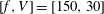$[f,V]=[150,30]$ on a chip with pits separated 500  $\unicode[STIX]{x03BC}\text{m}$ (corresponding to approximately 16 diameters) is chosen to illustrate the typical flow structure generated by an oscillating microbubble in the surrounding liquid. Since experiments are run with a low concentration of tracer particles, several repetitions are required to acquire significant statistics for each set of parameters. The particle trajectories shown in figure 2 correspond to several experiments and therefore different bubbles (approximately a dozen different ones in this particular case). The same data set is displayed in a movie available in the supplementary material.

Figure 2(a) corresponds to a three-dimensional view in the $(x,y,z)$ space of the bubble and particle trajectories, while figure 2(b) shows a projection in the $(x,y)$ space and 2(c) in the plane defined by the cylindrical coordinates $(\unicode[STIX]{x1D70C},z)$ . Particles are alternatively attracted (blue) and repelled (red) from the bubble, following loop-like trajectories in planes that are perpendicular to the chip, and establishing a ‘fountain-like’ flow pattern, as has been classically described by Miller (Reference Miller1988) and Marmottant & Hilgenfeldt (Reference Marmottant and Hilgenfeldt2003), among many others. The colour code in figure 2 corresponds to the radial component (in spherical coordinates) of the velocity field, $u_{r}$ . Positive values ( $u_{r}>0$ , red) indicate particles moving away from the bubble and negative values ( $u_{r}<0$ , blue) indicate that they are approaching to it. Particles velocity increase steeply as they move closer to the bubble and slow down to almost negligible values far away from it. Such large dynamic range becomes an experimental difficulty for tracking particles: those in the vicinity to the bubble move too fast to be tracked under our choice of recording frame rate, while particles separated by three bubble radii hardly move. Such a large velocity gradient is common in microbubble streaming systems, even with cylindrical bubbles (Miller & Nyborg Reference Miller and Nyborg1983; Marmottant & Hilgenfeldt Reference Marmottant and Hilgenfeldt2003; Marin et al. Reference Marin, Rossi, Rallabandi, Wang, Hilgenfeldt and Kähler2015). Due to this particularity of the flow field, its quantification becomes a non-trivial task. In what follows, we propose a method to characterize the flow by obtaining a ‘flow strength’ magnitude using well-known models in the literature that will allow us to characterize the entire streaming flow for different driving parameters and make proper comparisons.

The clear symmetry around the $z$ -axis shown by particle trajectories in figure 2(a,b) allows for a description of the flow in cylindrical coordinates $(\unicode[STIX]{x1D70C},z)$ (figure 2 c).

The Reynolds number (based on the bubble radius) varies significantly from values $Re<10^{-2}$ at distances $\unicode[STIX]{x1D70C}/a>2$ , to $Re\sim 1$ in the close vicinity of the bubble interface. Our experimental method does not permit us to track the inertial behaviour of particles in the near field, nor is that the aim of this study. For more information on this last regime, we refer to Thameem, Rallabandi & Hilgenfeldt (Reference Thameem, Rallabandi and Hilgenfeldt2016) who have recently studied the inertially driven migration of larger particles. In the following, we focus in the far-field region, where the flow field can be described as a Stokes flow using a streamfunction. Following the approach of Longuet-Higgins (Reference Longuet-Higgins1998), and using the method of images and singularity theory, the acoustic streaming flow can be obtained by assuming volumetric and translational oscillations of the bubble and applying the proper boundary conditions to obtain a streaming function. In this way, Marmottant & Hilgenfeldt (Reference Marmottant and Hilgenfeldt2003) used the method of images to consider the presence of the wall and obtained the leading-order streamfunction in the far field:

(3.1) $$\begin{eqnarray}\unicode[STIX]{x1D713}=-\frac{A_{f}}{r}\cos ^{2}(\unicode[STIX]{x1D703})\sin ^{2}(\unicode[STIX]{x1D703}),\end{eqnarray}$$

which accounts for the dipolar part (far field) of the full solution. $A_{f}$ is a constant, $r$ and $\unicode[STIX]{x1D703}$ are the distance from the bubble’s centre and the elevation expressed in spherical coordinates. The streamlines given by (3.1) are plotted in figure 3, together with the particle trajectories obtained experimentally. Notice that the latter follows the streamlines obtained from (3.1) very closely, as can be observed in the figure. Deviations of the particle trajectories from the streamlines occur mainly in the regions where the streaming velocity is lower and Brownian motion dominates the particle dynamics. The components of the velocity field in spherical coordinates can be thus easily obtained:

(3.2a,b ) $$\begin{eqnarray}u_{r}(r,\unicode[STIX]{x1D703})=-\frac{A_{f}}{r^{3}}\frac{\sin (2\unicode[STIX]{x1D703})\cos (2\unicode[STIX]{x1D703})}{\sin \unicode[STIX]{x1D703}},\quad u_{\unicode[STIX]{x1D703}}(r,\unicode[STIX]{x1D703})=-\frac{A_{f}}{r^{3}}\sin (\unicode[STIX]{x1D703})\cos ^{2}(\unicode[STIX]{x1D703}).\end{eqnarray}$$

Figure 3. Qualitative comparison of model and experimental data. Blue lines represent streamlines from the dipolar term of the full streamfunction employed to experimentally characterize the flow strength (3.1). Black dotted lines represent experimental data from the case study (150 kHz, 30 V). Deviations of the particle trajectories from the streamlines occur mainly in the regions where the streaming velocity is lower and Brownian motion dominates the particle dynamics. The data are projected in cylindrical coordinates, with $\unicode[STIX]{x1D70C}$ radial distance and $z$ height, both normalized over the bubble radius  $a$ .

Our approach to assess the flow strength consists of using $A_{f}$ as a fitting parameter: for each experiment, we find the value of $A_{f}$ that better fits the measured velocity field using expressions (3.2). A functional form for $A_{f}$ was proposed by Marmottant & Hilgenfeldt (Reference Marmottant and Hilgenfeldt2003) as

(3.3) $$\begin{eqnarray}A_{f}=B\unicode[STIX]{x1D716}^{2}a^{4}\unicode[STIX]{x1D714},\end{eqnarray}$$

where $\unicode[STIX]{x1D716}$ is the bubble’s relative amplitude of oscillation, $a$ is the bubble’s radius, $\unicode[STIX]{x1D714}$ the angular frequency $\unicode[STIX]{x1D714}=2\unicode[STIX]{x03C0}f$ , $f$ the driving frequency and $B$ is a constant that depends on the oscillation mode (Longuet-Higgins Reference Longuet-Higgins1998; Marmottant et al. Reference Marmottant, Versluis, De Jong, Hilgenfeldt and lohse2006). In a different configuration, Wang, Rallabandi & Hilgenfeldt (Reference Wang, Rallabandi and Hilgenfeldt2013) obtained the shape oscillations of a pinned cylindrical bubble at a wall and using an asymptotic model, they derived the frequency position and width of the bubble’s resonance peaks, which compared qualitatively well with experimental data. In the present work however, it is assumed that the bubble is oscillating in a low resonance mode, as in Marmottant et al. (Reference Marmottant, Versluis, De Jong, Hilgenfeldt and lohse2006). Although our model is simpler than that used by Wang et al. (Reference Wang, Rallabandi and Hilgenfeldt2013), the comparison shown here is strictly quantitative, as will be noticed later.

Thus, in our approach the flow strength is assessed by finding the value of $A_{f}$ (in a nonlinear least squares routine) that better fits the absolute velocity $|u|=\sqrt{u_{r}^{2}+u_{\unicode[STIX]{x1D703}}^{2}}$ with the functional form in (3.2). Note that the functional form employed for the velocity is only the dominant far-field term of the full streaming function, and therefore an approximation of the full one. This approximation is nonetheless justified since the majority of our measurements lay far from the bubble interface (a few bubble’s diameters), as can be observed in figures 2–4.

Figure 4. Quantitative comparison of the proposed fit from (3.2) with experimental data. (a) Particle trajectories used for the fit, plotted in cylindrical coordinates. (b) Comparison of the absolute velocity $|u|$ measured at different $z$ positions indicated in (a) with the corresponding fit. Velocity values are normalized with $u_{o}=a\cdot f$ . Although the model underestimates the velocities close to the bubble surface, it catches the overall trend of the velocity field. All data belong to the case of $f=150$  kHz and $V_{pp}=30$  V.

Figure 4 shows a comparison of the model with experimental data from the case under study (150 kHz, 30 V). The data are plotted in cylindrical coordinates for convenience, where $\unicode[STIX]{x1D70C}=r\sin (\unicode[STIX]{x1D703})$ and $z=r\cos (\unicode[STIX]{x1D703})$ , and normalized with the bubble radius $a$ . Figure 4(a) shows the positions where the particle velocity has been measured. Three $z$ -positions have been selected and highlighted to make a clear quantitative comparison with the model. In figure 4(b) the predicted (lines) and measured (points) velocity values are plotted together for the three different $z$ -positions that have been chosen as a function of the cylindrical radial position normalized with the bubble radius, $\unicode[STIX]{x1D70C}/a$ . The velocity is normalized using $u_{o}=a\cdot f$ , which is proportional to the expected fluid velocity close to the bubble’s surface $u_{s}=\unicode[STIX]{x1D716}^{2}a\unicode[STIX]{x1D714}$ . Wang et al. (Reference Wang, Rallabandi and Hilgenfeldt2013) as well as Marmottant et al. (Reference Marmottant, Versluis, De Jong, Hilgenfeldt and lohse2006) were able to achieve enough temporal and spatial resolution to measure the bubble’s oscillations and give and independent and precise estimation of $\unicode[STIX]{x1D716}$ . This is not the objective of the present manuscript and consequently we use $u_{o}$ instead of $u_{s}$ to normalize the velocities. In summary, the experimental data are well fitted with a single fitting parameter, the flow strength $A_{f}$ , which in this particular case takes the value 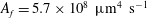$A_{f}=5.7\times 10^{8}~\unicode[STIX]{x03BC}\text{m}^{4}~\text{s}^{-1}$ .

As discussed above, most of the measured data lie in the range $\unicode[STIX]{x1D70C}/a>2$ , where the velocities are lower (typically $Re<10^{-2}$ ) and statistics are higher. Velocity increases rapidly as the particle approaches the bubble interface, reaching eventually $Re\sim 1$ if its streamline passes close enough to $\unicode[STIX]{x1D70C}/a\sim 1$ . Note that these regimes cannot be resolved using the current experimental settings and will not be discussed in this paper.

3.2 Bubble’s resonant frequency

In this section we make use of the streaming flow velocity to find the bubble’s resonant frequency in the range from 100 to 250 kHz, with a fixed driving voltage ( $V_{pp}=30$  V). The resonant frequency of the bubble oscillations is identified with the maximum in $A_{f}$ , which we can find independently of the natural acoustic resonances of the experimental system. Since the flow structure observed within the frequency range is similar to that shown in figure 2, the value of $A_{f}$ can be calculated as described in § 3.1.

The experimental values obtained for $A_{f}$ are plotted in figure 5(a) for the range of frequencies explored. A clear resonant frequency can be observed at $f=150$  kHz. Since no resonances have been found in the holder and chip system in this range of frequencies (see supplementary material), and $A_{f}$ depends quadratically on the bubble’s amplitude of oscillation (see (3.3)), we can conclude that microbubbles in pits of 30  $\unicode[STIX]{x03BC}\text{m}$ diameter have a natural resonance at $f=150$  kHz. Error bars based on the confidence bounds of the fitting are also plotted in figure 5, although difficult to see since the corresponding relative errors for $A_{f}$ are below 5 %. The coefficient of determination $R^{2}$ of the nonlinear fit gives valuable information on the fit, yielding values that go as high as 0.9 for $f=150$  kHz and as low as 0.3 for $f=100$  kHz.

Figure 5. (a) Streaming flow strength $A_{f}$ found experimentally as a function of the driving frequency for a driving voltage $V_{pp}=30$  V. Dashed lines are a guide to the eye. (b) Streaming flow strength $A_{f}$ as a function of the driving voltage for a driving frequency of 150 kHz. Circles represent experimental data and solid line is a fit of the form $A_{f}\propto V_{pp}^{2}$ . The inset represents the relative oscillation amplitude $\unicode[STIX]{x1D716}$ (indirectly obtained via the experimental flow field, more details in the text) for different driving voltages. The solid line is a linear fit to the data.

The resonant frequency value obtained experimentally can be compared with previous results in the literature. As a first approach, we can consider a free oscillating bubble immersed in an infinite volume of liquid in the case of small oscillations, which was discussed in the review by Plesset & Prosperetti (Reference Plesset and Prosperetti1977). Following linearization of the pressure field, and using Rayleigh’s bubble dynamic equation, an harmonic-oscillator type of equation with a natural resonance frequency takes the following general form:

(3.4) $$\begin{eqnarray}f_{o}=\frac{1}{2\unicode[STIX]{x03C0}a}\sqrt{\frac{3kP_{\infty }a-2\unicode[STIX]{x1D6FE}}{\unicode[STIX]{x1D70C}a}},\end{eqnarray}$$

which has been written in terms of the bubble radius $a$ , the liquid density $\unicode[STIX]{x1D70C}$ , its pressure at equilibrium $P_{\infty }$ , the liquid’s surface tension $\unicode[STIX]{x1D6FE}$ and the process’s polytropic exponent $k$ . In the case of small bubbles excited in our frequency range, it can be assumed that the process is isothermal (see the argument of Plesset & Prosperetti (Reference Plesset and Prosperetti1977)), and therefore $k\approx 1$ . The first summand in expression (3.4) corresponds to the Minnaert frequency, while the second term introduces a correction due to surface tension effects. Under such assumptions, and using our experimental parameters, one can obtain a $f_{o}=$ 182 kHz. That would be the expected result for a free bubble in a unbounded medium.

Miller & Nyborg (Reference Miller and Nyborg1983) obtained an approximate analytical expressions for the lowest resonance frequency of a bubble trapped in a micropore (equation (25) in their paper), assuming a semi-spherical and clamped (or pinned) bubble oscillating isothermally:

(3.5) $$\begin{eqnarray}f_{mn}=\frac{1}{2\unicode[STIX]{x03C0}a}\sqrt{\frac{15kP_{\infty }a+120\unicode[STIX]{x03C0}\unicode[STIX]{x1D6FE}}{32\unicode[STIX]{x1D70C}a}},\end{eqnarray}$$

which in this case yields a value of 151.5 kHz, very close to our measured value.

Recent studies have attempted to refine the predictions with more sophisticated techniques. Gelderblom et al. (Reference Gelderblom, Zijlstra, van Wijngaarden and Prosperetti2012) used a more general approach than Miller & Nyborg (Reference Miller and Nyborg1983) by assuming an arbitrary interface shape that was solved consistently in the limit of small amplitudes. Their results yield that the lowest resonant frequency for a pit in our same conditions should be close to 121 kHz. While Stricker (Reference Stricker2013) found a value of 123.5 kHz using level set simulations.

It is surprising that our results come closer to the somewhat simpler approach used by Miller & Nyborg (Reference Miller and Nyborg1983). Nonetheless, no conclusions can be drawn on the suitability of the different models unless more data become available for different pit sizes under the same experimental conditions. Such a set of experiments goes beyond the scope of the present paper. A possible reason to explain this agreement/disagreement is the shape of the bubble interface at rest: although we cannot know its exact real shape in our current set-up, it was clear that it had a certain convex curvature due to the light intensity gradients along its interface. All models and simulations described above (Miller & Nyborg Reference Miller and Nyborg1983; Gelderblom et al. Reference Gelderblom, Zijlstra, van Wijngaarden and Prosperetti2012; Stricker Reference Stricker2013) are however based on interfaces that are flat at rest. There is no literature to our knowledge dealing with the effect of the interface curvature on the bubble’s oscillation resonances.

In order to validate our method, we can compare our result with that obtained by Marmottant et al. (Reference Marmottant, Versluis, De Jong, Hilgenfeldt and lohse2006) by direct imaging of the bubble’s oscillations in a similar configuration. Using ultra-high-speed imaging to observe the oscillations of a bubble of $a=~20~\unicode[STIX]{x03BC}\text{m}$ at a driving frequency of $f=~190$  kHz, they obtained $\unicode[STIX]{x1D716}=0.077$ and $B=0.44$ , which yields 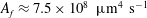$A_{f}\approx 7.5\times 10^{8}~\unicode[STIX]{x03BC}\text{m}^{4}~\text{s}^{-1}$ . The value lies very close to the $A_{f}$ obtained here using an experimental approach based on addressing the flow velocity, instead of the bubble’s oscillations. Therefore, we conclude that our experimental method can be used to probe the bubbles dynamics in a quantitative manner with no need of direct observation of the bubble’s oscillations, which typically requires both ultra-high speed and ultra-high magnification.

It is worth mentioning here that in the field of sonochemistry and ultrasonic cleaning (Fernandez Rivas et al. Reference Fernandez Rivas, Prosperetti, Zijlstra, Lohse and Gardeniers2010, Reference Fernandez Rivas, Verhaagen, Seddon, Zijlstra, Jiang, van der Sluis, Versluis, Lohse and Gardeniers2012b , Reference Fernandez Rivas, Stricker, Zijlstra, Gardeniers, Lohse and Prosperetti2013b ) the working frequency is typically chosen in a different way, mostly by finding an acoustic resonance of the system in which the acoustic energy is more efficiently transferred. Such a strategy has been followed by Fernandez Rivas et al. (Reference Fernandez Rivas, Prosperetti, Zijlstra, Lohse and Gardeniers2010, Reference Fernandez Rivas, Stricker, Zijlstra, Gardeniers, Lohse and Prosperetti2013b ) and Zijlstra et al. (Reference Zijlstra, Fernandez Rivas, Gardeniers, Versluis and Lohse2015) among others to induce nonlinear oscillations that will provoke the pinch-off of the main bubble into smaller ones. The sonochemical peak performance is typically achieved in such a regime, sometimes refereed as the high-power regime. Note that our experimental results have been obtained in the linear and harmonic-oscillations regime (low-power regime), and therefore they cannot be compared with those in sonochemistry. Nonetheless, using our experimental approach it is possible to discern easily and without high-speed imaging between linear and nonlinear oscillation regimes, as we will discuss in the next section.

3.3 Streaming flow dependence on the driving voltage

This section is dedicated to studying the response of the system to the driving voltage. For this set of experiments, we choose to maintain a constant driving frequency at its resonant value of 150 kHz and vary the driving voltage in a certain range. The minimum value of the driving voltage is chosen according to the acquisition parameters, i.e. at that voltage at which particle velocities are measurable. For technical reasons, this series of experiments was performed with thicker chips, and therefore is expected to yield lower bubble excitation for the same driving voltage as was done in the previous subsection.

The maximum value of the driving voltage in the measurement range is connected with the transition into the nonlinear regime and thus it can provide interesting information about the bubble dynamics. The driving voltage range to study goes from $V_{pp}=30$ to approximately 300 V. The particle trajectories within most of this regime are almost identical to those shown in figure 2 for 30 V, and therefore the value of the flow strength $A_{f}$ can be calculated as described in § 3.1.

The results are shown in figure 5(b), which shows a clear quadratic increase of the flow strength $A_{f}$ with the driving voltage. This is an expected result since the streaming flow, as a second-order effect, should scale with the oscillation amplitude as $u_{s}\propto \unicode[STIX]{x1D716}^{2}$ , which at the same time scales linearly with the driving voltage, i.e. $\unicode[STIX]{x1D716}\propto V_{pp}$ . With the obtained values of $A_{f}$ , we can use (3.3) to give an indirect estimation of the relative bubble’s amplitude of oscillation $\unicode[STIX]{x1D716}$ (taking $B=0.44$ , as directly measured by Marmottant et al. (Reference Marmottant, Versluis, De Jong, Hilgenfeldt and lohse2006) for a similar configuration). The values obtained in this way for the relative bubble oscillations lay in the range that have been typically observed for bubbles in the linear oscillation regime, i.e. $\unicode[STIX]{x1D716}\lesssim 0.2$ (Marmottant et al. Reference Marmottant, van der Meer, Emmer, Versluis, de Jong, Hilgenfeldt and Lohse2005; Garbin et al. Reference Garbin, Cojoc, Ferrari, Di Fabrizio, Overvelde, Van Der Meer, De Jong, Lohse and Versluis2007; Dollet et al. Reference Dollet, Van Der Meer, Garbin, De Jong, Lohse and Versluis2008). This is also consistent with our observations at higher voltages. For $V_{pp}>200$  V the bubble becomes unstable, no steady flow pattern can be observed and therefore measurements were scarce. We interpret such a lack of steadiness in the flow as the transition into the nonlinear oscillation regime, in which the bubble stability is compromised and the generation of daughter bubbles is likely to occur (Stricker et al. Reference Stricker, Dollet, Fernandez Rivas and Lohse2013; Zijlstra et al. Reference Zijlstra, Fernandez Rivas, Gardeniers, Versluis and Lohse2015). Such a dramatic change in the flow behaviour is a clear advantage of this experimental approach: the transition into the nonlinear regime can be easily found in this way since it is very reproducible for different experimental runs.