


1. Introduction
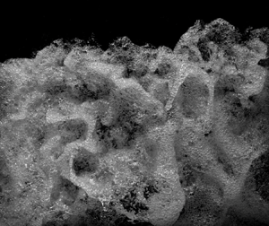
In highly turbulent free-surface flows, the presence of strong motions generates a continuous interaction between the gas and liquid phases, characterised by the formation of complex and rapidly varying flow features, leading to enhanced surface roughness, breakup and disintegration (Hino Reference Hino1961; Peregrine Reference Peregrine1981; Ervine & Falvey Reference Ervine and Falvey1987; Brocchini & Peregrine Reference Brocchini and Peregrine2001a). These flows are of extreme complexity, characterised by substantial air entrainment, violent free-surface motion, intensive turbulent mixing and large vortex advection, as shown in figure 1(a) for the Qiantang River tidal bore in China and in figure 1(b) for an oscillatory hydraulic jump at the entrance of a minimum energy loss (MEL) culvert during a flash flood in May 2009 in Brisbane, Australia. In addition, these turbulent flows were believed to be responsible for the movement of large boulders during severe storms (Bressan et al. Reference Bressan, Guerrero, Antonini, Petruzzelli, Archetti, Lamberti and Tinti2018). An understanding of the fluid mechanics behind these convoluted turbulent processes is critical for a variety of domains, including effective flood protection measures, safe and reliable hydraulic structures, coastal resilience and optimised design of ship vessels.

Figure 1. (a) Tidal bore on the Qiantang River, China, on 11 October 2014. (b) Oscillating hydraulic jump at Norman Creek minimum energy loss (MEL) culvert during a flash flood in May 2009 in Brisbane, Australia. (Photographs by Prof. H.Chanson.)
Brocchini & Peregrine (Reference Brocchini and Peregrine2001a,Reference Brocchini and Peregrineb) described a number of deformations of the free surface, which were induced by turbulence beneath the water surface. By considering the stabilising effects of gravity and surface tension, the notion of weak free-surface turbulence (WFST) and strong free-surface turbulence (SFST) was established. WFST is associated with small Froude and Weber numbers, and it is characterised by little or no disturbance of the free surface, without any air entrainment. Recently, the physical processes associated with WFST were investigated numerically (Shen & Yue Reference Shen and Yue2001; Fulgosi et al. Reference Fulgosi, Lakehal, Banerjee and De Angelis2003; Guo & Shen Reference Guo and Shen2010; Yamamoto & Kunugi Reference Yamamoto and Kunugi2011), experimentally (Smolentsev & Mirachaie Reference Smolentsev and Mirachaie2005; Savelsberg & Van De Water Reference Savelsberg and Van De Water2008, Reference Savelsberg and Van De Water2009; Seol & Jirka Reference Seol and Jirka2010) and theoretically (Hunt & Graham Reference Hunt and Graham1978; Teixeira & Belcher Reference Teixeira and Belcher2002; Magnaudet Reference Magnaudet2003; Hunt, Stretch & Belcher Reference Hunt, Stretch and Belcher2011).
Depending on the roles of gravity and surface tension, and therefore on the Froude and Weber numbers, different behaviours of the free surface can be observed. Flows with dominant surface tension result in small capillary waves with possible occurrence of micro-breakers (Banner & Peregrine Reference Banner and Peregrine1993; Lin & Rockwell Reference Lin and Rockwell1995; Duncan et al. Reference Duncan, Qiao, Philomin and Wenz1999). Gravity-dominated flows are characterised by local breakings, observed in self-aerated open channel flows and surface waves with the generation of ‘scars’ and ‘boils’ (Jackson Reference Jackson1976; Chanson Reference Chanson1997; Kiger & Duncan Reference Kiger and Duncan2012). In the case of SFST, the flow motion is strong enough to overcome both gravity and surface tension, leading to surface deformations, breaking and large air entrainment, with the formation of liquid droplets and sprays (Ervine & Falvey Reference Ervine and Falvey1987; Brocchini & Peregrine Reference Brocchini and Peregrine2001a; Yu et al. Reference Yu, Hendrickson, Campbell and Yue2019). These features are complex and rapidly varying phenomena, induced by an even more complicated process occurring within the flow, below the surface.
Because of the complexity of the process, the literature on SFST is small compared to WFST. A series of theoretical works by Hong & Walker (Reference Hong and Walker2000), Brocchini & Peregrine (Reference Brocchini and Peregrine2001b) and Brocchini (Reference Brocchini2002) modelled SFST using Reynolds-averaged Navier–Stokes equations and averaged boundary conditions. Experimentally, SFST was mainly examined in hydraulic jumps and transient breaking bores because of their highly dissipative nature. Mouaze, Murzyn & Chaplin (Reference Mouaze, Murzyn and Chaplin2005) focused on the length scales of SFST in hydraulic jumps, while surface fluctuations and the coupling with air–water flow properties have been the object of multiple studies, including Chanson & Brattberg (Reference Chanson and Brattberg2000), Murzyn, Mouaze & Chaplin (Reference Murzyn, Mouaze and Chaplin2007), Chachereau & Chanson (Reference Chachereau and Chanson2011) and Wang (Reference Wang2014). In unsteady bores, Leng & Chanson (Reference Leng and Chanson2015) examined the free-surface characteristics of the breaking roller toe, while Wüthrich, Shi & Chanson (Reference Wüthrich, Shi and Chanson2020a) provided comprehensive datasets of free-surface profiles and strong turbulent fluctuations using image processing techniques based on ultra-high-speed videos. Numerical simulations of SFST are rare due to the large computational power required by the high Reynolds numbers associated with these two-phase turbulent flows ( $\sim$10 $^{5}$). Lubin & Glockner (Reference Lubin and Glockner2015) performed a large-eddy simulation (LES) of the shoaling process of breaking waves, showing the existence of aerated vortical structures responsible for air–water interchange on the free surface. These filaments were later visualised by Lubin et al. (Reference Lubin, Kimmoun, Veron and Glockner2019) using ultra-high-speed videos. Recently, several studies have revealed great details on the bubble–turbulence interplay in breaking waves (Deike, Melville & Popinet Reference Deike, Melville and Popinet2016; Wang, Yang & Stern Reference Wang, Yang and Stern2016; Chan, Johnson & Moin Reference Chan, Johnson and Moin2020a; Chan et al. Reference Chan, Johnson, Moin and Urzay2020b). Mortazavi et al. (Reference Mortazavi, Le Chenadec, Moin and Mani2016) performed direct numerical simulations (DNS) of a hydraulic jump, showing the bubble advection process in the shear layer, which interacted with the free surface. Yu et al. (Reference Yu, Hendrickson, Campbell and Yue2019) conducted a DNS investigation of a free-surface flow, showing the dependence of air entrainment on different Froude and Weber numbers.
Despite these recent contributions, advances in the numerical modelling of SFST have remain limited. In part, this can be attributed to the lack of detailed experimental studies focusing on air–water interfacial features. Experimental investigations of SFST remain a challenge because of the randomness of the process, the limitations of available instruments and data processing techniques. In this context, this research presents a pioneering study in the experimental characterisation of SFST in breaking bores, generated by the sudden closure of a gate in an initially steady flow (§ 1.1). The goal is to provide qualitative and quantitative descriptions of surface turbulence using visual observations of ultra-high-speed video data and an extension of the optical flow (OF) technique to the free-surface velocity fields. Because of the unsteadiness of the process, these results rely on ensemble statistics based on multiple repetitions. More specifically, this research:
(i) identified recurring air–water surface features in SFST within breaking bores;
(ii) presented a detailed characterisation of the physical behaviour of these features in terms of their geometrical properties, duration and frequency of appearance; and
(iii) applied an OF technique to the free surface, detecting the fluid motion associated with SFST, to further investigate their turbulent and energy dissipation properties.
1.1. Breaking bores
This study focused on SFST in breaking bores. These unsteady flows are commonly observed in the environment, including breaking waves, rejection surges in channels and rivers induced by the operation of hydropower plants, flood waves, tidal bores, dam-break waves and tsunamis propagating in rivers (Henderson Reference Henderson1966; Treske Reference Treske1994; Chanson Reference Chanson2011a). Bores are best described by their Froude number,
 \begin{equation} Fr_1 = \frac{V_1 + U}{\sqrt{g \dfrac{A_1}{B_1}}}, \end{equation}
where  $V_1$ is the initial velocity of the steady flow (positive downstream), $U$ is the bore celerity (positive upstream), $g$ is the gravitational constant ( $g = 9.8$ m s $^{-2}$), $A_1$ is the cross-sectional area of initial flow and $B_1$ is the free-surface width. Bores with Froude numbers slightly above unity are associated with undular waves ( $1 < Fr_1 < 1.4$), whereas, for $Fr_1> 1.5 - 1.6$, a breaking phenomenon occurs (Leng & Chanson Reference Leng and Chanson2017).
For these bores, the steepening wave front eventually falls down because of gravity, inducing a shoaling process that generates a velocity shear between the front and the initial flow. This triggers a continuous rolling motion of the front, responsible for the bore propagation (Lubin et al. Reference Lubin, Kimmoun, Veron and Glockner2019). This region marking the sudden change between the initially steady flow and the propagating bore is called the ‘roller toe’, and is shown in figure 2. The rolling motion entrains air into the bore, forming large air pockets immediately downstream of the roller toe, which are further broken up into finer air bubbles in the developing shear layer (Leng & Chanson Reference Leng and Chanson2019a). The velocity shear also triggers Kelvin–Helmholtz instabilities within the roller toe region, providing the primary source of vorticity in the breaking bore (Hornung, Willert & Turner Reference Hornung, Willert and Turner1977). The turbulent structures formed in the roller toe region evolve to large-scale vortices, which are advected downstream together with entrained air bubbles. The advected vortices eventually dissipate, and the entrained bubbles are then driven upwards by buoyancy. During the advection phase, secondary entrainment and de-aeration processes occur because of the interactions between vortices and the free surface (Nezu & Nakagawa Reference Nezu and Nakagawa1993; Wang & Chanson Reference Wang and Chanson2016; Wüthrich et al. Reference Wüthrich, Shi and Chanson2020a). The interaction between this convoluted motion within the roller and the free surface generates substantial SFST, resulting in a number of recurring and rapidly evolving foamy structures (Wüthrich, Shi & Chanson Reference Wüthrich, Shi and Chanson2020b). Bubbles in the aerated region range in size from the submillimetric scale to tens of centimetres (Leng & Chanson Reference Leng and Chanson2019a), and they are known to play crucial roles in several phenomena, including an increase in the mixture flow bulk and an enhancement in the air–water mass transfer (Ervine & Falvey Reference Ervine and Falvey1987; Wood Reference Wood1991; Chanson Reference Chanson1997). The reproduction of bores in the laboratory (figure 2, inset) pointed out similarities with field observations, revealing the presence of a number of complex air–water surface features whose behaviour remains widely unexplored. Thus, a deep understanding of the physical process within the breaking roller is necessary, motivating the experimental nature of this study.
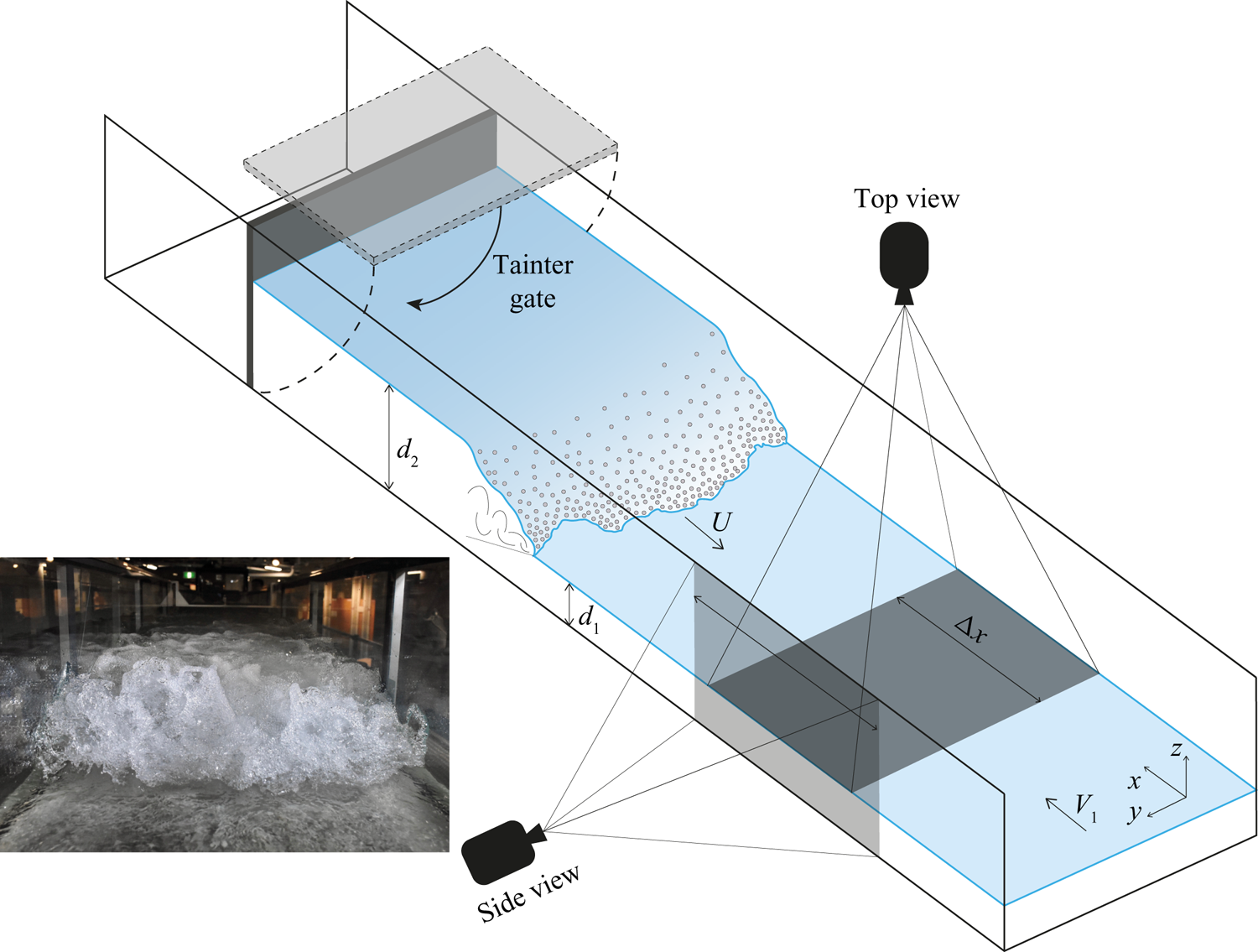
Figure 2. Schematic of the bore generation technique and experimental set-up. Inset: breaking bore in the hydraulic laboratory ( $Fr_1 = 2.4$).
2. Experimental set-up
2.1. Experimental facility
All experiments were performed in a large-size facility at the University of Queensland, Australia. A steady flow was induced in a 19 m long, 0.7 m wide and 0.5 m high channel with an adjustable bottom slope. The channel had a smooth PVC invert with glass sidewalls to optimise flow visualisation. Water was introduced into the channel through an upstream tank equipped with flow straighteners, baffles and a three-dimensional (3-D) convergent. At the downstream end, the flow was evacuated through an overfall, avoiding any backwater effect. The bore generation was achieved through the sudden closure of a Tainter gate, inducing a positive surge travelling towards the upstream section of the channel (figure 2). Previous studies by Leng & Chanson (Reference Leng and Chanson2017) on the same facility reported closure times of less than 0.2 s for all repetitions, showing excellent repeatability of the bore characteristics (bore front arrival time, bore height, bore celerity), independently of the operator and day of the experiment.
2.2. Instrumentation
The water discharge was set to 0.1 m $^{3}$ s $^{-1}$, measured through a magneto flow meter with an accuracy of 10 $^{-5}$ m $^{3}$ s $^{-1}$. A Phantom ultra-high-speed video camera (v2011) was used to capture the bore motion, recording at 22 000 frames per second (f.p.s.) with a resolution of $1280~\text {pixels} \times 800~\text {pixels}$. The camera was installed either on the side or on top of the channel, as shown in figure 2. All videos were recorded at a fixed reference location $x = 8.5$ m from the channel inlet, ensuring a fully developed breaking bore. For all configurations, the camera was fixed and did not move with the bore. For the side-view experiments, the Phantom video camera was equipped with a Zeiss $^{\text{TM}}$ Planar T* 85 mm $f$1.4 lens, located at a distance of $\sim$1.5 m from the channel sidewall, allowing a measuring window of $0.52~\text {m} \times 0.32~\text {m}$, resulting in a pixel resolution of $\sim$0.3–0.4 mm. For the top view, the Phantom video camera was installed above the channel (perpendicular to the channel flow), equipped with a Nikkor $^{\text{TM}}$ AF 50 mm $f$1.4 lens, located at a distance of $\sim$1.3 m above the free surface of the initial flow, allowing the capture of all its width with a measuring window of $0.7~\text {m} \times 0.45$–0.52 m (figure 2). This resulted in a resolution ranging from 0.60 to 0.65 mm pixel $^{-1}$, for all top-view videos. Both prime lenses had a negligible degree of barrel distortion, i.e. $\sim$0.087 % (Zeiss) and $\sim$1.3 % (Nikkor). Video recording was performed with a light-emitting diode (LED) array, model GS Vitec MultiLED (cold white 7700 lm), to maximise the illumination of the flow features, avoiding any resonance with the high-speed-video camera. For each flow condition 25 top-view videos were recorded, with average durations ( $\pm$ standard deviation) of 1.203 s ( $\pm$0.073 s) for $Fr_1 = 2.4$, of 1.027 s ( $\pm$0.060 s) for $Fr_1 = 2.1$ and of 0.526 s ( $\pm$0.015 s) for $Fr_1 = 1.5$. The three durations of the videos depended on the different bore flow celerities (table 1). For side-view experiments, eight videos were recorded per Froude number, as these were only used to track the trajectories of the water droplet in the $x$–
$x$– $z$ plane.
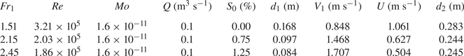
Table 1. Physical properties of the breaking bores investigated in the present study.
2.3. Flow conditions
The present study is based on a Froude similitude. The use of the same fluid also guaranteed a similitude in terms of Morton number  $Mo = g\mu ^{4}/(\rho \sigma ^{3})$, with $\mu ,\ \rho$ and $\sigma$ being the fluid dynamic viscosity, density and surface tension, respectively. The experiments were conducted at large Reynolds numbers $Re = \rho (V_1 + U)d_1/ \mu$, guaranteeing a physically meaningful extrapolation to prototype data with minimum scale effects (Leng & Chanson Reference Leng and Chanson2017). Experimental tests were performed on three bores with Froude numbers $Fr_1 = 1.5$, 2.1 and 2.4, as detailed in table 1. All bores propagated in the upstream direction with a bore front celerity $U$, against a steady flow characterised by an initial water depth $d_1$ and a flow velocity $V_1$.
3. Methodology
Detailed visual observations of the SFST revealed the presence of well-defined, 3-D air–water surface structures interacting with the flow, with length scales varying from 0.0001 m (bubble size, as reported by Leng & Chanson (Reference Leng and Chanson2019a)) up to 0.7 m (channel width). Typical surface features are introduced in figures 3 and 4. Herein, the following simple distinction is introduced:
(i) Millimetric flow features: size between $\sim$0.3 mm (pixel size) and 5 mm.
(ii) Macroscopic flow features: size larger than 5 mm.


Figure 3. Definition sketch of the main air–water surface features identified within SFST on breaking bores.

Figure 4. Typical length and velocity scales of main turbulent air–water surface features observed in breaking bores. Present data are plotted against the length–velocity graph by Brocchini & Peregrine (Reference Brocchini and Peregrine2001a).
This study focuses on macroscopic air–water surface features for which the behaviour is not dominated by capillarity processes, inclusive of water droplets ejected from the roller, with diameters between 1 and 10 mm. All features, identified and discussed in § 4, are composed of a number of smaller entities, mostly air–water structures (bubbles, drops, foam), with a behaviour and properties interacting at smaller scales. A schematic representation and a brief definition of the main air–water surface features identified in the present study is presented in figure 3, with further details provided in § 4.
The ultra-high-speed videos allowed for a detailed characterisation of the temporal and spatial behaviour of the air–water surface features. Although some air–water surface features have been reported in other multiphase flows, at present no detailed classification of these features is available in the literature. Given the complex and random flow motion associated with rapid and unpredictable changes in both space and time, all flow features were identified manually. Manually acquired data were then analysed in terms of ensemble median properties, to reduce the influence of potential human error. For each air–water surface feature, its lifespan (or duration) was measured as the time difference between appearance and disappearance, i.e. when the feature could no longer be recognised. Video analyses showed that most flow features tended to expand during the first half of their lifespan, before shrinking. At their maximum expansion, their geometrical properties, i.e. characteristic lengths and widths, were manually measured and statistically analysed. In addition, 30 crowns and 30 fingers for  $Fr_1 = 2.4$ were randomly chosen and manually tracked every 150 frames (i.e. 0.0068 s), providing an insight into the evolution of their geometrical properties. The accuracy of the measurements depended on the pixel size, here calculated to be 0.3–0.4 mm for the side-view videos and 0.60–0.65 mm for the top-view videos at the elevation of the initial free-surface flow $d_1$. Temporal measurements depended on the video acquisition frequency (22 kHz), resulting in an accuracy of $4.5\times 10^{-5}$ s. Although time-consuming and subject to potential human error, these manual measurements guaranteed the best reliability and quality control.
Altogether, the geometrical properties, their evolution, durations and frequencies were used to provide a quantitative description of the flow features in § 5. These results are combined in § 6 with velocity fields on the surface of the roller, obtained though OF techniques. This triggered some discussion in terms of the features’ turbulent properties and energy dissipation in § 7.
4. Air–water flow features
Breaking bores visually presented a highly turbulent roller with an enhanced surface roughness and a large amount of air entrainment and entrapment (figure 5). Herein, the chaotic behaviour of the air–water mixture in the free surface of the roller toe revealed short-lived, highly energetic, rapidly evolving and 3-D surface features, as documented in the top-view images presented in figure 5 for the breaking rollers with  $Fr_1 = 1.5$, 2.1 and 2.4. These features were the result of a complex flow motion strongly linked to the physical processes occurring within the roller (i.e. below the surface), revealing the complexity of their geometry and the interactions that occurred between these features.

Figure 5. Top view of the strong surface turbulence observed in breaking rollers with different Froude numbers. Bore propagation from bottom to top.
The SFST was deemed responsible for the formation of a number of recurring macroscopic features, shown in figures 3 and 4. A closer look showed that these features were made of a foamy mixture of air and water entities. During their lifespans, these interfacial surface features evolved in both space and time, interacting with each other, before disappearing within the roller. Video analyses showed that, during their motion, features often merged with each other, without generating splashes. The latter might be explained by the low momentum linked to their foamy nature. The coalescence of the air–water flow features resulted in a rearrangement of the interfacial structures and the formation of new features. Thus, the average length scale of the features was a time-dependent variable. The duration (or lifespan) of these features was less than one second, making ultra-high-speed data a requirement for a comprehensive visual assessment. While all features were characterised by a chaotic nature and a random process, some recurring features were identified (figure 3) and are detailed hereafter. The classification of these features was based on repeated visual observations, assessing the shape, the dynamics and the location where these features occurred. Ejections that were completely detached were identified as ‘droplets’. Protrusions that remained attached to the roller were classified as thin ‘fingers’, ‘thumbs’ or flat and semicircular ‘crowns’. A number of upstream projections occurred at the roller toe, with shapes that visually looked like circular ‘mushrooms’ and chaotic ‘spider webs’. Because of the abrupt motions within the roller, some air cavities were observed and classified as ‘holes’. The recirculating pattern induced up-flows with circular surface outbreaks characterised by a ‘boiling’ behaviour, therefore identified as ‘boils’. The main length and velocity scales of these features were also compared to the heuristic approach by Brocchini & Peregrine (Reference Brocchini and Peregrine2001a) in figure 4, confirming the strong turbulent behaviour of breaking bores.
4.1. Fingers
Fingers were elongated monoaxial ejections in which the length ( $L$) was significantly greater than the width ( $W$), with $L/W>2$ (figures 3 and 6). Fingers were the result of an upward ejection of an air–water volume with an impulsive and highly energetic behaviour. Selected examples of fingers observed for various Froude numbers are presented in figure 6(a).
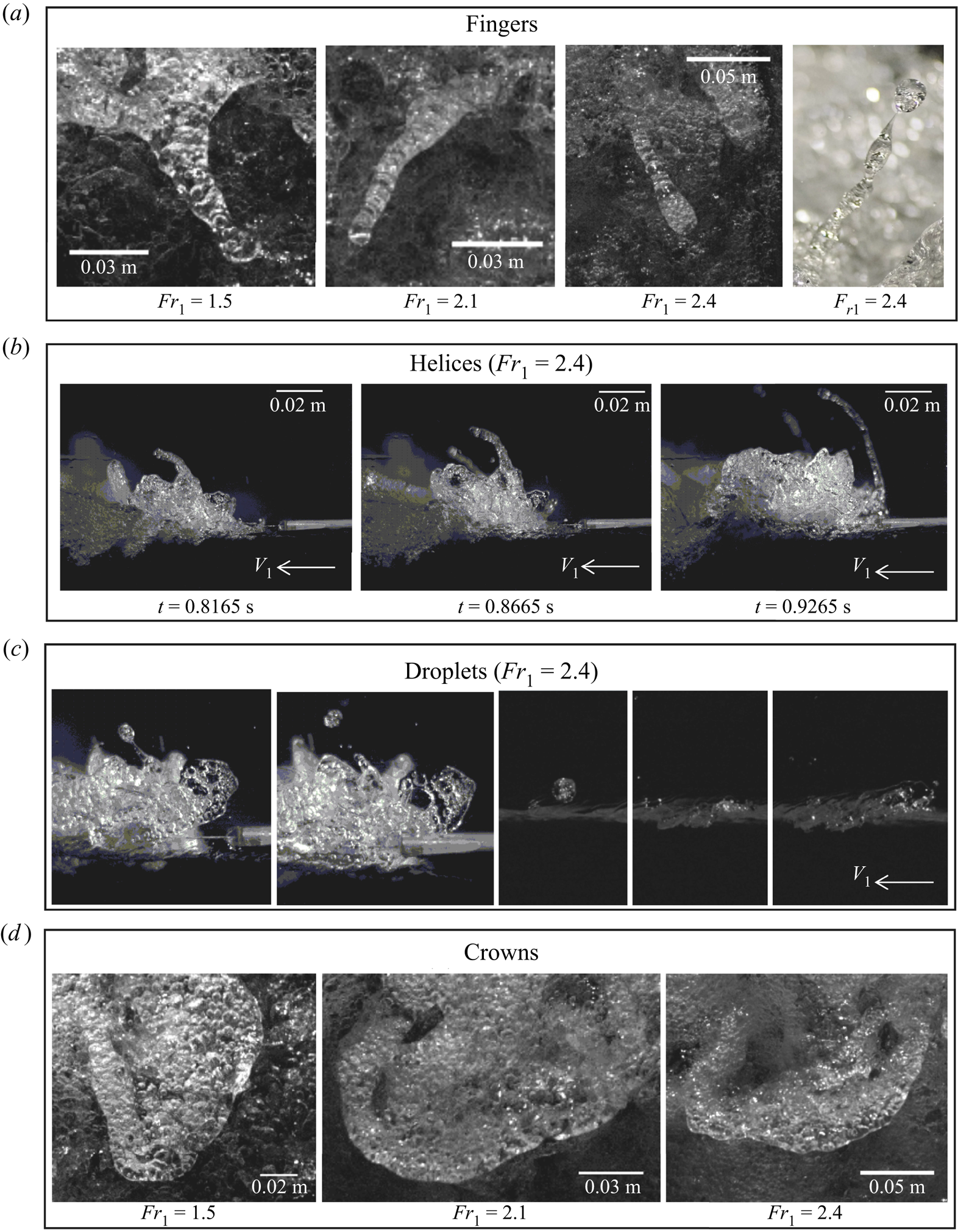
Figure 6. Images of fingers, helices, droplets and crowns.
Visual observations showed that fingers occurred predominantly in the first half of the roller, close to the roller toe. Fingers were mostly directed in the streamwise direction, and opposite to the propagation of the bore roller, not unlike similar features observed in high-velocity water jets discharging into air (Brennen Reference Brennen1970; Hoyt & Taylor Reference Hoyt and Taylor1977; Chanson Reference Chanson1997). Detailed observations revealed that fingers were made of smaller bubbles, with a single bubble occasionally occupying the whole finger width (figure 6a). During their lifespan, the main body of the finger elongated with reducing cross-sectional area, possibly under the combined influence of gravity and surface tension. During the motion, fingers showed the appearance of Plateau–Rayleigh instabilities, partially responsible for their breakage into smaller droplets of lower total surface area (Lubin et al. Reference Lubin, Kimmoun, Veron and Glockner2019). When the evolution of the finger did not reach a critical thickness to trigger the pitching process, the feature either merged with the surrounding flow or sank back into the roller's main body. Side-view videos showed that some particular fingers had a pseudo-cylindrical shape, attributed to a rotational motion, similar to ‘helices’ (figure 6b). For these, the uneven distribution of the mass along the axis of the helix could favour breakage processes and the ejection of water droplets. For all Froude numbers, some thick fingers with  $L/W\sim 1$ were also observed and classified as ‘thumbs’. These were not as common as other fingers with $L/W>2$ and could be associated with highly aerated protuberances emerging from the air–water mixture.
4.2. Water droplets
Water droplets were relatively small and detached ejections of air–water mixtures above and in front of the roller free surface. The generation process of these droplets was hard to assess, although a particular type of water droplets resulted from the rotating behaviour of the fingers (or helices), generated by the uneven distribution of the mass along their axis. During a breakage event, the finger locally became progressively thinner until capillary instabilities pinched off the ligament and the newly formed droplets separated (Notz & Basaran Reference Notz and Basaran2004). Upon separation, surface tension reshaped the droplets and the threads were retracted. Overall, breakage was a very quick phenomenon (Soligo, Roccon & Soldati Reference Soligo, Roccon and Soldati2019) and an example is presented in figure 6(c). The ejected droplet followed a parabolic trajectory in accordance with projectile motion, further discussed in § 5.1. Side-view videos showed that the majority of these droplets were ejected against the steady flow with an initial velocity that was greater than the bore front celerity, thus contributing to the propagation upstream of the roller toe. The impact of the droplet on the upstream free-surface flow induced some local splashes, as shown in figure 6(c), in line with previous studies on breaking bores (Leng & Chanson Reference Leng and Chanson2015; Wang, Leng & Chanson Reference Wang, Leng and Chanson2017; Leng & Chanson Reference Leng and Chanson2019b) and hydraulic jumps (Murzyn & Chanson Reference Murzyn and Chanson2009; Chanson Reference Chanson2011b).
4.3. Crowns
Crowns were surface features generated by air–water ejections with a pseudo-semicircular shape, where its length was smaller than its width, i.e.  $L/W<1$. Examples of crowns are presented in figure 6(d) for several Froude numbers. Crowns were characterised by a protrusive nature while they emerged from the roller and visually presented a relatively lower content of air bubbles, compared to fingers and thumbs. Their spatial evolution mostly developed against the bore direction and presented a quasi-two-dimensional (quasi-2-D) evolution in time with a spreading behaviour. At the end of their lifespan, the crowns sank back into the roller or merged with other features. For $Fr_1=1.5$, the crowns were weaker and some were unable to generate a protrusion that emerged from the flow, generating surface scars, especially in the back of the roller where turbulence was gravity-driven.
4.4. Slugs
Slugs were defined as S-shaped cords of foamy mixture, primarily observed along the direction of the propagating roller. Examples are shown in figure 7(a) for all tested Froude numbers ( $Fr_1 = 1.5$, 2.1 and 2.4). Slugs were foamy entities characterised by a very high local concentration of air bubbles, resulting in locally higher void fractions. Slugs followed the shape of curvilinear lines and some slugs with multiple bends would result in more complicated features. In addition, some slugs presented bendings that were characterised by the presence of highly aerated protuberances, previously identified as thumbs (§ 4.1).
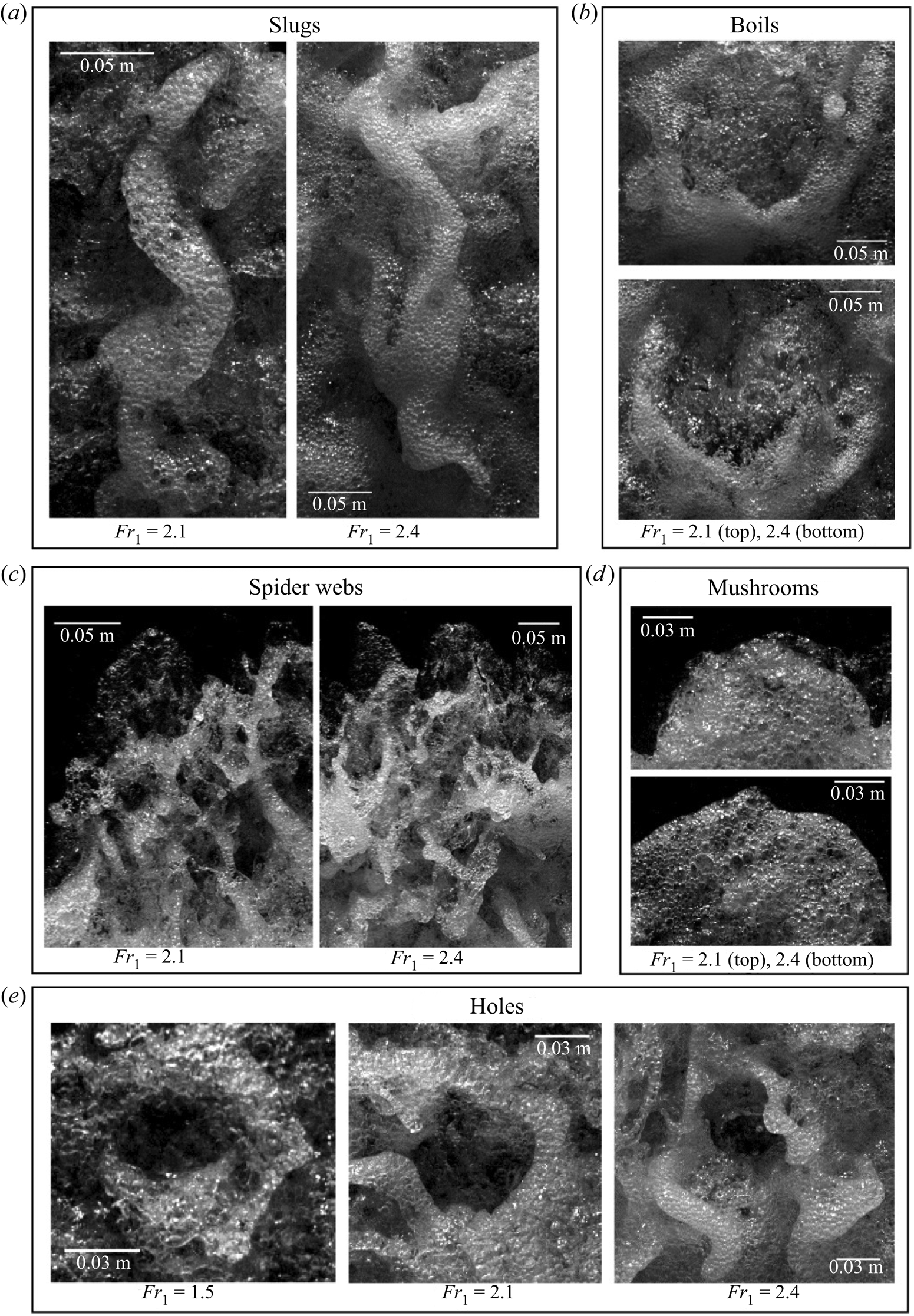
Figure 7. Images of slugs, boils, mushrooms, spider webs and holes.
4.5. Spider webs
Spider webs were very short-lived features, resulting from the complex interaction between multiple features including fingers, droplets and other foamy structures. This complex connectivity resulted in a mesh of thin structures and holes, assuming the form of a spider web (figure 7). Video observations revealed that spider webs only occurred in the first half of the roller, closer to the bore front. The spider web shared certain similarities with the development of hairpin vortices in parallel shear flows (Wu & Moin Reference Wu and Moin2009; Eitel-Amor et al. Reference Eitel-Amor, Örlü, Schlatter and Flores2015). Because of their short duration, the shape of these features evolved very quickly, leading to a jagged profile of the roller toe perimeter (figure 7c). Often these features followed the ejections of a mushroom (§ 4.6). Their rapid disappearance within the incoming flow was sometimes responsible for the local backward motion of the roller toe, previously observed by Leng & Chanson (Reference Leng and Chanson2015, Reference Leng and Chanson2019b), Wang et al. (Reference Wang, Leng and Chanson2017) and Wüthrich et al. (Reference Wüthrich, Shi and Chanson2020a). Spider webs occurred for all tested Froude numbers, but they appeared less well defined for lower Froude numbers ( $Fr_1 = 1.5$) and more aeration seemed to be associated with stronger bores ( $Fr_1 = 2.1$ and 2.4).
4.6. Mushrooms
Mushrooms consisted of an accumulation of a pseudo-circular foamy mixture of air and bubbles towards the roller toe, as shown in figure 7(d). The foamy features presented a semicircular shape, in which the width  $W$ was nearly double the length $L$, i.e. $W\sim 2L$, thus taking the shape of a mushroom cap. These features presented a thin layer of wet foam with heterogeneous bubble size distributions for all tested Froude numbers, spreading from the roller toe, as a secondary bore on the free surface. Similarly to spider webs, they were short-lived and rapidly evolved into new features.
4.7. Boils
Boils were annular patterns resulting from an upward flow motion reaching the free surface from within the roller. Visually these features presented a higher concentration of bubbles and foam on the outer ring, with a relatively clear water core inside, where boiling bubbles could be observed (figure 7b). Boils were observed for all tested Froude numbers and they mostly appeared in the downstream half of the roller (figure 8), where the flow was visually less aerated and gravity regained an important role. In comparison to other features, their evolution was slower in time, implying a longer lifespan. Boils appeared both on the centreline and next to the sidewalls, and their final diameter could reach more than half of the channel width ( $W\sim 0.5B$). At low Froude numbers, boils sometimes appeared to be somewhat similar to crowns. However, these hybrid features did not present any upward ejections nor a protrusive nature, probably because the roller did not contain enough energy to eject a full crown. Boils (or bursts) were previously identified by Jackson (Reference Jackson1976) in various natural rivers, including the Polomet (Russia), where length scales $0.27 < L_x/d < 0.57$ were documented by Korchokha (Reference Korchokha1968). Boils also induced motions similar to the scars identified by Brocchini & Peregrine (Reference Brocchini and Peregrine2001a), confirming a link between boils and gravity-driven flows in figure 4.

Figure 8. Location of the air–water surface features analysed in the present study for  $Fr_1= 2.4$, where $x_r$ is the mean longitudinal position of the roller toe perimeter (Appendix B).
4.8. Holes
Holes were 3-D and short-lived air cavities within the bore roller surface, surrounded by other features. These appeared for all tested Froude numbers and were characterised by a darker colour, i.e. clear water beneath the air cavity. Holes were associated with mostly circular shapes, with a length comparable to the width ( $L \sim W$). Visual examples are provided in figure 7(e).
4.9. Summary
The previous subsections have shown that different features occurred at different locations within the roller's upper surface. The longitudinal and transverse coordinates of a number of air–water features were documented in figure 8 with respect to the ensemble-averaged position of the roller toe, detailed in Appendix B. The location of the surface features referred to their centroid at the time of maximum development. Overall, these data confirmed that more surface features occurred towards the roller toe and little to almost no features were observed near the sidewalls. The appearance of the droplets was dominant near the roller toe, with some produced in the middle of the roller and no droplets observed in the lower part. Mushrooms were rarer compared to other features, only observed along the roller toe perimeter, whilst spider webs occurred just downstream of the roller toe, where the free surface was discontinuous in the  $x$–
$x$– $y$ plane. Fingers and crowns covered the top and bottom halves of the roller, respectively. Boils were mainly located away from the roller toe, while slugs and holes were observed in the middle of the roller. Overall, figure 8 showed a clear partitioning of the features within the roller, probably associated with their different physical properties, hydrodynamic behaviours and energy levels, further investigated in §§ 5 and 6.
5. Quantitative analysis of most common flow features
A number of recurring air–water surface features associated with the SFST were identified within the breaking bore roller for different Froude numbers in § 4. Herein a quantification of their physical properties is developed, based on 25 ultra-high-speed videos, each recorded at 22 000 f.p.s. Such a quantitative description allowed for a better insight into the SFST, providing data in support of the validation of numerical simulations. It is important to point out that the appearance of these features was completely random in both space and time. Because of their short duration and rapid variation, the use of a pattern recognition software was not considered for maximum reliability and optimum quality control. All videos were processed manually and the features were identified on a frame-by-frame basis. Specifically, this section analyses the physical behaviour of these air–water surface features in terms of (1) size, (2) frequency, (3) duration and (4) location within the roller. Hereafter only the most frequent features are quantitatively described, namely water droplets, fingers, crowns and holes. The remaining features were too random or rare to provide a meaningful statistical analysis.
5.1. Water droplets
Water droplets of different sizes were constantly ejected during the propagation of the bore. The majority of these droplets were observed in the first part of the roller (figure 8), where the interaction between the different features was visually more intense. A number of droplets were also ejected in the upstream part of the flow, colliding with the incoming steady flow (figure 6c). From the side-view videos, the trajectories of some water droplets were manually identified from ejection to disappearance for  $Fr_1= 2.4$ and 2.1. Measurements were taken every 0.01 s and spatial positions referred to the centre of gravity of the moving droplet. Bores for $Fr_1 = 2.1$ and 2.4 had different propagation celerities, which means that the duration of the videos was not identical for the two flow conditions, resulting in 85 water droplets for $Fr_1 = 2.4$ and 45 for $Fr_1 = 2.1$. Owing to their limited number, droplets for $Fr_1 = 1.5$ were not considered. All experimental trajectories captured for $Fr_1 = 2.4$ and 2.1 are presented in figure 9(b) in normalised form, showing an excellent agreement with the ballistic equation of projectile motion with negligible air friction:
 \begin{equation} Z ={-}\frac{1}{2}\frac{g}{v_{0,X}^{2}}X^{2}+\frac{v_{0,Z}}{v_{0,X}}X, \end{equation}
where  $Z$ and $X$ are the local vertical and horizontal directions with the reference system shifted where the droplet ejection occurred (figure 9a), $g$ is the gravitational constant ( $g = 9.8$ m s $^{-2}$), and $v_{0,X}$ and $v_{0,Z}$ are the horizontal and vertical components of the initial ejection velocity of the droplet. Note that $X$ and $v_{0,X}$ are defined to be positive in the upstream direction, in line with the bore front celerity $U$. When air resistance is neglected and gravity only acts in the vertical direction, the components of the droplet velocity are $v_{0,X}=v_0\cos {\theta }$ and $v_{0,Z}=v_0\sin {\theta }-0.5gt^{2}$, where $v_0$ is the total droplet initial velocity $v_0 = (v_{0,X}^{2} + v_{0,Z}^{2})^{0.5}$, $\theta$ is the ejection angle with respect to the horizontal direction and $t$ is the time since the ejection. A comparison of the experimental points with the coefficients in (5.1) allowed $v_{0,X}$, $v_{0,Z}$ and $\theta$ to be estimated for each ejected water droplet.

Figure 9. (a) Definition sketch of the water droplet trajectory's main parameters. (b) Normalised ballistic trajectories for water droplets observed for  $Fr_1 = 2.4$ (85 trajectories) and $Fr_1 = 2.1$ (45 trajectories).
The statistical distributions of the ejection angles  $\theta$ with respect to the horizontal direction are presented in figure 10(a). Note that all trajectories were analysed in the $X$–
$X$– $Z$ plane (streamwise direction) and any transverse motion was not considered. The results showed that the ejection angles ranged between 16.8 $^{\circ }$ and 83.1 $^{\circ }$ for $Fr_1 = 2.4$, and between 2 $^{\circ }$ and 65.6 $^{\circ }$ for $Fr_1 = 2.1$. In addition, the statistical distributions for both Froude numbers suggested possibly two dominant modes for the droplet ejection angle around 30 $^{\circ }$ and 45 $^{\circ }$.

Figure 10. Statistical distributions of (a) ejection angles, (b) components of the droplet's instantaneous ejection velocities ( $Fr_1 = 2.4$) and (c) droplet size $d$ (
$d$ ( $Fr_1 = 2.1$ and 2.4).
The statistical distributions of the droplets’ vertical ( $v_{0,Z}$) and horizontal ( $v_{0,X}$) components of the initial velocity are presented in figure 10(b) for $Fr_1 = 2.4$, normalised with the bore front celerity $U$. Figure 10(b) revealed a marked peak, which was approximately 1.5 times the bore front celerity. This finding demonstrated that droplets travelled faster than the bore front, and could interact with the upstream steady flow, not unlike field observations by Leng & Chanson (Reference Leng and Chanson2015) and Wang et al. (Reference Wang, Leng and Chanson2017) in the tidal bores of the Qiantang and Garonne rivers. In addition to the high energetic level near the bore front, further analysed in § 6, this phenomenon is likely to be associated with a combined effect of velocity fluctuations within the roller and a rotating motion associated with a number of surface features, including fingers and helices (figure 6b,c).
The size of the droplets ejected during the bore motion was measured through side-view videos for  $Fr_1 = 2.1$ and 2.4. The statistical distributions are presented in figure 10(c), showing a mode in droplet diameter between 2.5 and 3 mm for both flow conditions, with an average value of 3.3 mm for $Fr_1 = 2.4$ and 2.8 mm for $Fr_1 = 2.1$. Although based on a limited number of samples, the result hinted that stronger bores could eject slightly larger droplets.
5.2. Fingers
Fingers were elongated features and their appearance was manually detected in 25 top-view videos for each Froude number ( $Fr_1 = 1.5$, 2.1 and 2.4), focusing on their geometrical properties, durations and frequencies. The majority of fingers were located in the first half of the roller and characterised by a relatively short duration. The data showed that the total number of detected fingers decreased for lower Froude numbers, with a population of 100 for $Fr_1 = 1.5$ compared to 163 for $Fr_1 = 2.4$. Although fingers appeared in all videos, the number of features detected per video was random and ranged from two to 12 for all $Fr_1$. An estimation of the frequency of appearance of fingers was obtained as the ratio between the total number of features and the total duration of all videos. A larger number of fingers was detected for higher Froude numbers, but these were associated with lower bore front celerities and thus longer video durations. This led to similar frequencies $\sim$4.5 Hz for all flow conditions.
Fingers were relatively short-lived features with a lifespan  $T_{span}$ of 0.10–0.15 s. The probability density functions (p.d.f.) of lifespan are presented in figure 11(a) in dimensionless form for all tested $Fr_1$, showing shorter median durations for lower Froude numbers, thus suggesting a different temporal scale for turbulent structures on the free surface.

Figure 11. Statistical distributions for different Froude numbers of (a) a finger's lifespan ( $T_{span}$), normalised using the bore's initial flow depth $d_1$, flow velocity $V_1$ and celerity $U$, and (b) the ratio between the finger's length and width $L/W$ at maximum elongation.
The fingers’ main geometrical properties were also investigated, being characterised by their length  $L$ and width or thickness $W$, with ratios $L/W>2.0$. Herein $L$ and $W$ were measured for all detected fingers at their maximum elongation. Since figures 3 and 6(a) showed that $W$ was not constant over the whole finger's length, it was measured at half length. The statistical distributions of the ratio $L/W$ are presented in figure 11(b), showing decreasing median values for lower Froude numbers. Furthermore, the p.d.f. distribution of $L/W$ showed a more pronounced asymmetry, with increasing skewness values, for larger Froude numbers.
To characterise the unsteady nature of these features, the air–water boundaries of 30 randomly chosen fingers were manually tracked every 150 frames (i.e. 0.0068 s) for  $Fr_1= 2.4$, capturing the temporal evolution of their main geometrical properties. Herein, only a selected example of the time evolution of feature boundaries is shown in figure 12, while a complete dataset was presented by Wüthrich et al. (Reference Wüthrich, Shi and Chanson2020b). Figure 12(a) shows the development of an individual finger on top of the free surface. This temporal variation involved a stretching process: an increase in finger length and a reduction in width. Figure 12 also shows an ensemble median analysis of the geometrical properties of all 30 manually tracked fingers. This approach was similar to that used by Nikora et al. (Reference Nikora, Habersack, Huber and McEwan2002) for sediment particle diffusion over a channel bed. Note that the droplets were not taken into account once detached from the finger's main body. The time evolution of the finger perimeter and enclosed area were shifted to the same relative time, such that $t-t_0 = 0$, where $t_0$ was the starting time of the feature. Figure 12(b) presents the ratio of the number of available fingers $N_{c}$ to the total number of fingers ( $N = 30$). The ensemble median properties were extracted only when $N_{c}/N > 0.5$, leading to $(t-t_0)V_1/d_1 < 2.25$, as shown by the red curve. The evolution of the finger perimeter $P$ and enclosed area $A$ are shown in figures 12(c) and 12(d), showing an overall increase of the ensemble median values over time. Some features showed a parabolic-shaped behaviour, thus suggesting a reduction in finger size towards the end of their lifespan.

Figure 12. Typical example of time evolution of the same finger. (a) Air–water boundaries. Time evolution of length and enclosed area of air–water flow boundary for fingers with  $Fr_1 = 2.4$. (b) The ratio of available finger number ( $N_c$) to total finger number ( $N$). (c) Normalised perimeter for 30 fingers and their ensemble median values. (d) Normalised area for 30 fingers and their ensemble median values. Here $t_0$ is the starting time of the feature.
Helices were a particular type of finger characterised by a twisting motion. Manual tracking of the helix from the side-view videos (figure 13) revealed that even the tip of the finger followed a parabolic trajectory in the longitudinal direction (i.e. plane  $X$–
$X$– $Z$), typical of ballistic motions (§ 5.1). This is shown in figure 13 for $Fr_1 = 2.4$, where the thin solid line represents the instantaneous side-view contour of the helix, whilst the thick black line shows the external trajectory followed by the head of the helix. Figure 13 also shows good agreement with the ballistic trajectory described in (5.1) (dotted line).

Figure 13. Example of trajectory followed by helices for  $Fr_1 = 2.4$; the thin solid line represents the instantaneous side-view contour of the helix, whilst the thick black line shows the external trajectory followed by the head of the helix. The dotted line shows the comparison with the ballistic trajectory in (5.1).
5.3. Crowns
Crowns were 3-D features emerging from the roller, with a clearly marked air–water perimeter (figure 6). These had a semicircular shape with a length  $L$ smaller than the width $W$ (i.e. $L/W < 1$). In contrast to fingers, crowns were mostly observed in the second half of the roller (figure 8). The process to characterise the behaviour of the crowns was similar to that applied to fingers. For the same 25 videos per Froude number, crowns showed frequencies $\sim$3.5–4.2 Hz, which were slightly lower than fingers. The lifespan of the crowns, $T_{span}$, from appearance to disappearance, was systematically recorded for all features, and statistical distributions in figure 14(a) revealed lower median durations for lower Froude numbers. A statistical analysis of the crowns’ main geometrical features $L$ and $W$ is presented in figure 14(b), where the ratio of crown length to width ( $L/W$) showed similar median values for all Froude numbers, thus suggesting that the shape was not strongly affected by the flow conditions. The p.d.f. seemed to have a more symmetrical behaviour for smaller Froude numbers, with increasing skewness for larger values, thus suggesting a more circular behaviour at larger Froude numbers.
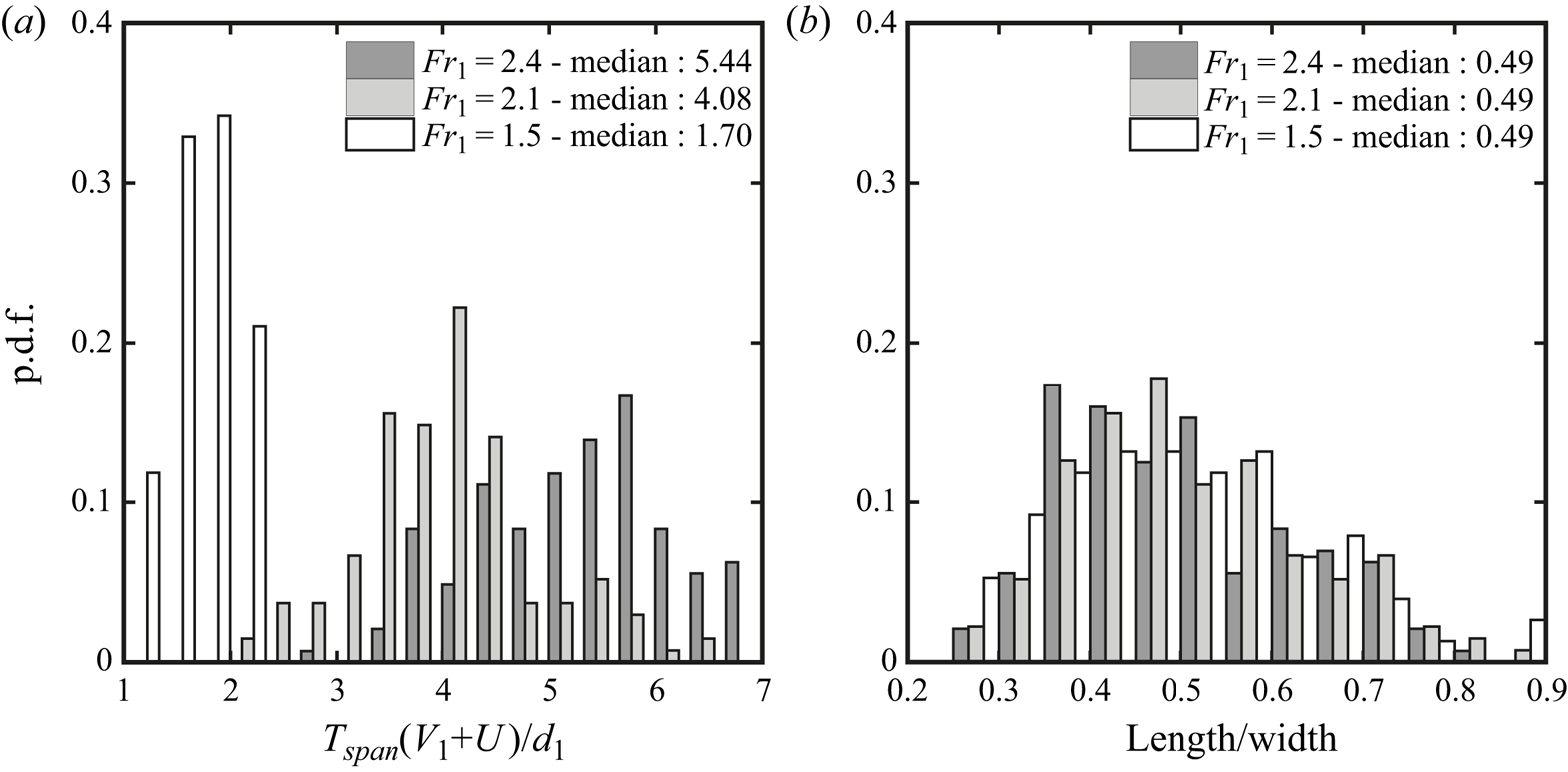
Figure 14. Statistical distributions for different Froude numbers of (a) a crown's lifespan ( $T_{span}$), normalised using the bore's initial flow depth $d_1$, flow velocity $V_1$ and celerity $U$, and (b) the ratio between the crown's length and width $L/W$ at maximum elongation.
Thirty randomly chosen crowns were manually tracked across their lifespan for  $Fr_1 = 2.4$, providing typical examples of time evolutions of the air–water boundaries. An example is presented in figure 15(a), while more examples can be found in Wüthrich et al. (Reference Wüthrich, Shi and Chanson2020b). The crown increased in size with time up to a maximum value at $t = 0.068$ s, before gradually shrinking. The crown initially showed a high density of air bubbles, but tended to stretch further apart during the spreading process. The manually tracked air–water boundaries were used to compute the statistical distributions of the boundary arclength and enclosed area for $Fr_1 = 2.4$, following the approach of Nikora et al. (Reference Nikora, Habersack, Huber and McEwan2002). Given the different lifespan of these features, the ensemble median was calculated when the instantaneous population encompassed at least 50 % of the dataset, i.e. for $N_{c}/N > 0.5$ or $(t-t_0)V_1/d_1 < 2.75$. The results are plotted in figures 15(c) and 15(d), with the ensemble median values represented by the red curves. The majority of crowns had an increasing perimeter and enclosed area with time, resulting in overall increasing values of the ensemble median. On the other hand, some crowns experienced a right-skewed parabolic shape for the arclength and enclosed area, corresponding to a slow decay process.

Figure 15. Typical example of time evolution of the same crown. (a) Air–water boundaries. Time evolution of length and enclosed area of air–water flow boundary for fingers with  $Fr_1 = 2.4$. (b) The ratio of available finger number ( $N_c$) to total finger number ( $N$). (c) Normalised perimeter for 30 fingers and their ensemble median values. (d) Normalised area for 30 fingers and their ensemble median values. Here $t_0$ is the starting time of the feature.
5.4. Holes
Holes were a characteristic feature of the roller consisting of transient air cavities induced by the continuous changes within the surface of the roller. The variability of the SFST induced openings in the roller, characterised by a darker colour (viewed in elevation), as compared to the other foamy structures. These were numerous throughout the roller's upper surface, more frequent in the first half of the roller (leading), as compared to the second half (trailing), as shown in figure 8. The appearance of holes within the roller was random and a selection of four holes per video, resulting in a total of 100 samples per Froude number, were randomly analysed. For each feature, the total duration from appearance to disappearance was recorded, along with the surface properties (length  $L$ and width $W$), at approximately half of its lifespan. The results showed that holes were very short-lived, with lifespans $T_{span}$ shorter that 0.1 s for all tested Froude numbers. Statistical analyses of the available dataset are presented in figure 16, revealing distributions with a symmetrical behaviour for all Froude numbers. Similarly to previous findings for crowns, this suggested that the shape was not affected by the bore's initial flow condition and was linked to other hydrodynamic processes occurring on the surface of the roller. In addition, holes revealed a narrower lifespan distribution at lower Froude numbers. Some geometrical assessment of selected holes revealed ratios of $L/W$ with a relatively symmetrical shape and a peak around $L/W\sim 1$ at all flow conditions, implying that holes had a mostly circular shape.

Figure 16. Statistical distributions for different Froude numbers of (a) a hole's lifespan ( $T_{span}$), normalised using the bore's initial flow depth $d_1$, flow velocity $V_1$ and celerity $U$, and (b) the ratio between hole length and width $L/W$.
6. Surface velocity and turbulence statistics
The free-surface characteristics were quantitatively described using an OF technique for the breaking bore with  $Fr_1 = 2.4$. The OF is the distribution of apparent motion of objects between consecutive frames. In air–water flows, the OF detected the motion of air–water interfaces, thus providing an estimation of interfacial velocities. The reader is referred to the detailed description and validation of the OF in Appendix A.
The surface OF field derived from the top view provided a description of the 2-D flow motion at different free-surface elevations. In the absence of a 3-D reconstruction of OF fields, the current approach represents a simplified, yet effective, method to physically examine the dynamics of the free-surface velocity in a complicated 3-D air–water flow. However, it is important to point out that these data only provide a semi-quantitative description of the flow field motion within the SFST, since it was impossible to clearly ascertain the elevation of the OF data. An example of instantaneous velocity fields for  $Fr_1 = 2.4$ is presented in figure 17, confirming the presence of strong flow motions in the $x$–
$x$– $y$ plane, with the occurrence of complicated turbulent structures, including the air–water features identified in § 4.
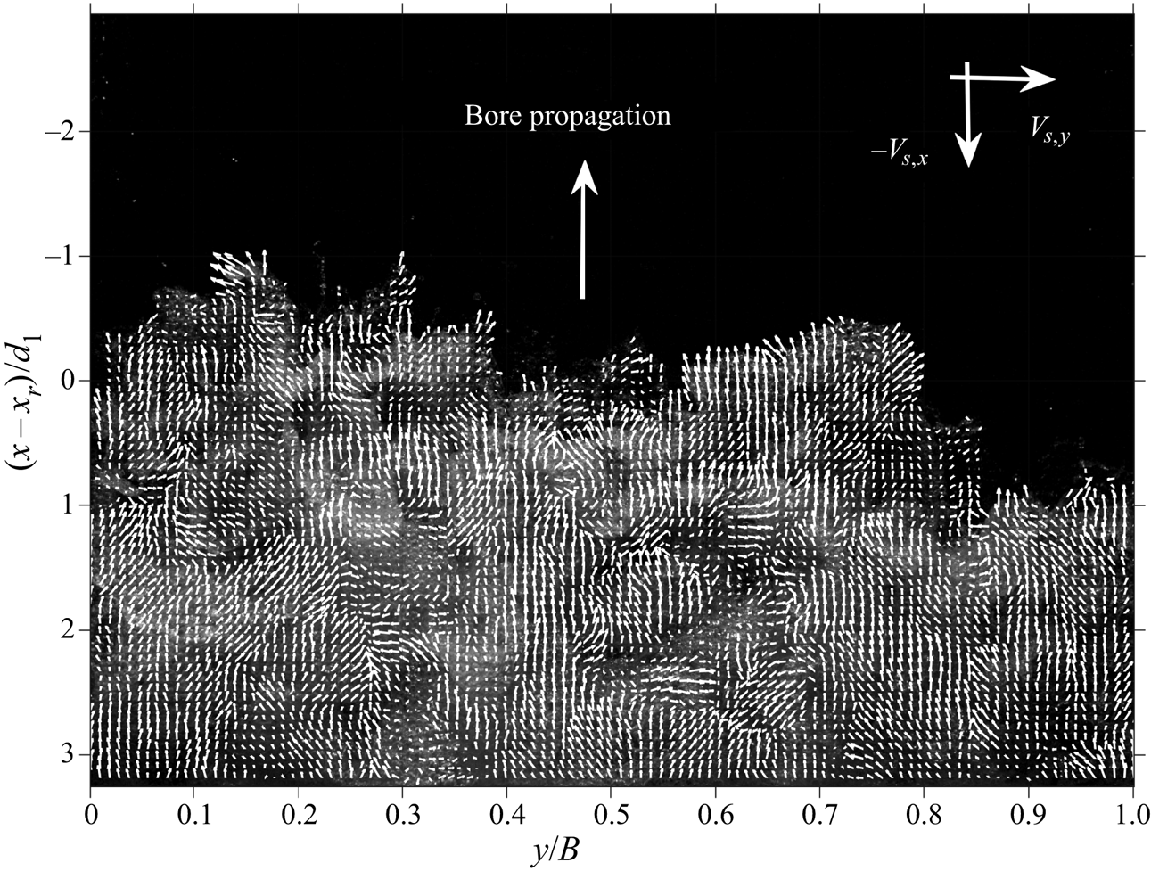
Figure 17. Instantaneous surface velocities obtained from the application of the OF technique to the top-view high-speed videos ( $Fr_1 = 2.4$).
6.1. Instantaneous velocity fields of fingers and crowns
The instantaneous velocity fields in the region around fingers and crowns were isolated, allowing for a more detailed characterisation of the kinematic behaviour of these features within the surrounding flow. The data in figure 18 revealed complex velocity fields around the fingers, including rapid changes in the direction of the velocity vector between two time steps, with the development of strong vortical structures. The transverse velocity became the predominant component near the pinching region of the finger. Two common finger behaviours were identified: (1) divergent and (2) merging. The divergent behaviour indicated a spreading process, whilst the merging behaviour suggested that a finger formed from the interaction of nearby features. The same procedure was applied to crowns, revealing a strong spreading process within the feature, thus explaining the behaviour observed through manual tracking in figure 15. A strong discontinuity with the surrounding vector fields was observed near the boundaries of these features; however, since the top view only described a 2-D motion, such behaviour was only partially assessed and the interactions with the small-scale structures was hard to interpret. Additional examples of velocity fields around fingers and crowns can be found in Wüthrich et al. (Reference Wüthrich, Shi and Chanson2020b).
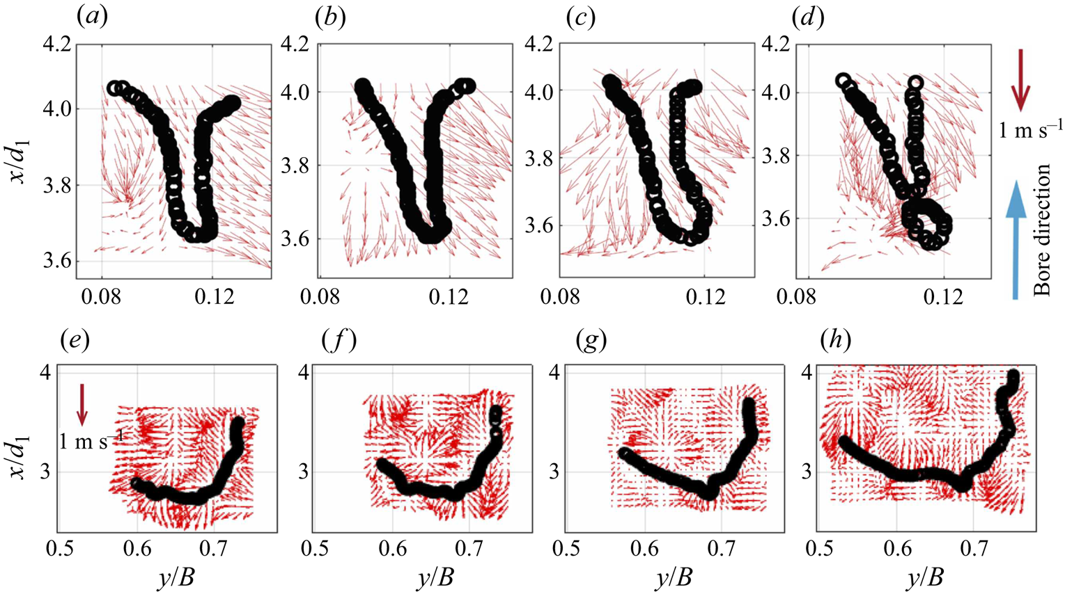
Figure 18. Flow fields obtained with the surface OF technique around a finger (a–d) and a crown (e–h). The time lapse between panels was  $t = 0.014$ s.
6.2. Ensemble-averaged velocities and energy considerations
The ensemble-averaged surface OF velocity fields were obtained based upon 25 videos, using a synchronisation technique detailed in Appendix B. Figures 19(a) and 19(b) present the ensemble-averaged longitudinal  $\langle V_{S,x} \rangle$ and transverse $\langle V_{S,y} \rangle$ components of the velocities, with the number of frames available for ensemble statistics in figure 19(c). The validation of these surface velocities was achieved based on previous experimental data by Wüthrich et al. (Reference Wüthrich, Shi and Chanson2020a), as detailed in Appendix A.2. Overall, the longitudinal ensemble-averaged velocities $\langle V_{S,x} \rangle$ presented negative values, indicating a bore motion propagating in the upstream direction, in agreement with visual observations. The longitudinal velocity data also showed a decrease in absolute value behind the roller toe in the downstream direction, with large variations observed near the roller toe region. This is in line with previous measurements within and beneath the roller by Leng & Chanson (Reference Leng and Chanson2017) and Wüthrich et al. (Reference Wüthrich, Nistor, Pfister and Schleiss2018). In the transverse direction, the absolute values of the ensemble-averaged velocity $\langle V_{S,y} \rangle$ were smaller compared to the longitudinal data. The data showed the presence of transverse motions, with the surface flow attempting to move away from the sidewalls. This might be explained by the development of large structures reflected by the sidewalls towards the centreline, confirming the 3D nature of the surface flow. Nevertheless, the longitudinal and transverse velocity components data showed, respectively, symmetrical and mirrored distributions with respect to the centreline.

Figure 19. The ensemble-averaged free-surface OF velocity fields: (a) longitudinal component  $\langle V_{S,x} \rangle$; (b) transverse component $\langle V_{S,y} \rangle$; and (c) number of available frames for ensemble statistics, $N_{ave}$.
Turbulence statistics were further extracted from the ensemble-averaged and instantaneous velocity data. The root-mean-square (r.m.s.) velocity fluctuations were defined as  $v_{{rms},i} = \sqrt {\langle v_{S,i} ^{2} \rangle } / V_1$, where $v_{S,i}$ are the longitudinal ( $i = x$) or transverse ( $i = y$) surface velocity fluctuations. The ratio of transverse and longitudinal velocity fluctuations $v_{{rms},y} / v_{{rms},x}$ provided information on the homogeneity of the free-surface turbulence. The distribution in figure 20(b) showed a strong symmetry with respect to the channel centreline. The longitudinal component dominated close to the sidewalls, where the transverse flow motion was constrained. This confirmed that, in the regions $y/B < 0.05$ and $y/B> 0.95$, the approximation of 2-D turbulence was acceptable, in line with previous studies using particle image velocimetry and image-based techniques near the sidewall in breaking waves and hydraulic jumps (Huang et al. Reference Huang, Hsiao, Hwung and Chang2009; Shi, Leng & Chanson Reference Shi, Leng and Chanson2020). Further away from the sidewalls, the ratios $v_{{rms},y} / v_{{rms},x} > 0.75$ indicated a more homogeneous free-surface turbulence, while the wide region around the centreline was dominated by fluctuations in the longitudinal direction.

Figure 20. Turbulence statistics using ensemble-averaged velocity: (a) TKE  $k$ and (b) the ratio of r.m.s. transverse $v_{{rms,}y}$ and longitudinal $v_{{rms,}x}$ velocity fluctuations.
Since the present measurements only provided 2-D data in the  $x$–
$x$– $y$ plane, the turbulent kinetic energy (TKE) was estimated using the standard approximation by Svendsen (Reference Svendsen1987) and Kimmoun & Branger (Reference Kimmoun and Branger2007) for breaker-generated turbulence:
 \begin{equation} k = \frac{4}{3} \frac{(v^{2}_{{rms,}x} + v^{2}_{{rms,}y})}{2}.\end{equation}
The distribution of  $k$ is presented in figure 20(a), showing relatively high energy values in the thin strip shape along the roller toe perimeter, induced by the strong shear between the initial flow and the propagating bore. This suggested that the roller toe acted as a linear source of turbulence generation, in agreement with Hornung et al. (Reference Hornung, Willert and Turner1977), who showed that the roller toe was a line generator of air entrainment and vorticity. Longitudinally, the energy data decayed rapidly away from the roller toe, suggesting a strong energy dissipation process highly linked with the SFST and the generation of surface features identified in § 4. Downstream of the roller, the high-energy regions enclosed a region with lower and more constant energy values. These findings will be discussed with the flow features in § 7.
The energy dissipation rate  $\epsilon$ is a key parameter for the dynamics of two-phase flows (Hinze Reference Hinze1955; Deane & Stokes Reference Deane and Stokes2002), and for a Newtonian fluid it is defined as
 \begin{equation} \epsilon = \nu \left\langle \frac{\partial v_i}{\partial x_j} \left(\frac{\partial v_i}{\partial x_j} + \frac{\partial v_j}{\partial x_i}\right)\right\rangle, \end{equation}
where  $i,j = x,y,z$, and $\nu$ is the local kinematic viscosity of the two-phase flow, which varies with the void fraction. Since the rapidly varying free surface hindered the measurements of void fraction, the viscosity of water was adopted for the calculation of the dissipation rate. The unsolved components in (6.2) were estimated using the assumption that vertical derivatives have similar average magnitudes to the longitudinal and transverse ones (Doron et al. Reference Doron, Bertuccioli, Kats and Osborn2001), resulting in an estimation of $\epsilon$ from in-plane data as
 \begin{align} \epsilon &= \nu \left[4 \left\langle \left(\frac{\partial v_x}{\partial x}\right)^{2} \right\rangle + 4 \left\langle \left(\frac{\partial v_y}{\partial y}\right)^{2} \right\rangle+3 \left\langle \left(\frac{\partial v_y}{\partial x}\right) ^{2} \right\rangle + 3 \left\langle \left(\frac{\partial v_x}{\partial y}\right) ^{2} \right\rangle \right. \nonumber\\ &\quad \left. + \, 4\left\langle \frac{\partial v_x}{\partial x} \frac{\partial v_y}{\partial y} \right\rangle +6 \left\langle \frac{\partial v_x}{\partial y} \frac{\partial v_y}{\partial x} \right\rangle\right]. \end{align}
The data of the energy dissipation rate are presented in figure 21(a), showing consistent results with the kinetic energy data, with high dissipation near the roller toe and rapid decay in the longitudinal direction. This magnitude and trend agreed well with the side-view phase-averaged data of Huang et al. (Reference Huang, Hsiao, Hwung and Chang2009). This hinted at a strong link between the generation of air–water surface features near the roller toe and energy dissipation.

Figure 21. Energy dissipation on the bore free surface: (a) turbulence dissipation rates; and (b) the ratio of turbulence dissipation rate to total energy dissipation rate.
Following Stive (Reference Stive1984), the mean energy flux  $E$ in a bore was defined as
 \begin{equation} E = \int \int \langle p + \rho g \xi + \tfrac{1}{2} \rho(V_x ^{2} + V_y ^{2} + V_z ^{2} )V_x \rangle \,\text{d}z\,\text{d}y, \end{equation}
where  $p$ is the pressure and $\xi$ is the vertical distance from the surface. The first and second terms represent the pressure components and were estimated to be zero for the free-surface flow. The third term is the mean kinetic energy. Thus, the total dissipation rate was defined as
 \begin{equation} e_V ={-} \frac{\partial E}{\partial x \partial y \partial z} ={-} \frac{1}{2} \frac{\partial}{\partial x}\rho \langle (V_x ^{2} + V_y ^{2} + V_z ^{2})V_x \rangle. \end{equation}
Herein, a constant water density  $\rho$ was used, though the density varied due to the void fraction. The vertical velocity component near the surface was not measured in the present study, and the ensemble-averaged vertical velocity field was extracted from the work of Shi et al. (Reference Shi, Leng and Chanson2020), who computed the 2-D velocity field in the $x$–
$x$– $z$ plane in a bore with a similar Froude number ( $Fr_1 = 2.1$) using the same OF technique. An approximation of (6.5) was
 \begin{equation} e_V \approx{-} \rho ( \langle (V_x ^{2} + V_y ^{2})V_x \rangle + \langle V_z \rangle ^{2} \langle V_x \rangle ) . \end{equation}
 The ratio  $\rho \epsilon / e_V$ represented the contribution of turbulence dissipation to total energy dissipation, as presented in figure 21(b). The ratio distribution exhibited similar distributions with the dissipation and TKE data. It was found that the turbulence dissipation near the roller toe reached up to 20 % of the total energy dissipation, consistent with the 18 % for a fully turbulent bore in the surf zone by previously obtained by Huang et al. (Reference Huang, Hsiao, Hwung and Chang2009).
6.3. Integral time and length scales
The integral length and time scales characterise the spatial and temporal dimensions of the turbulence generated during the breaking process. These parameters were derived using the cross-correlation analysis of surface OF velocity fields (§ 6.1). The cross-correlation time scale  $T_{R,i}$ was calculated as the integral of the cross-correlation function for both velocity components in $x$ and $y$, from its peak value to the first zero-crossing, as
 \begin{equation} T_{R,i} = \int_{\tau (R_i = R_{i,{max}})}^{\tau (R_i = 0)} R_i (\tau)\,\text{d}\tau, \end{equation}
where  $\tau$ is the time lag, $R_i$ is the cross-correlation function and $R_{i,{max}}$ is the maximum value of the cross-correlation function. For each velocity component, the integral turbulent length ( $L_i$) and time ( $T_i$) scales were further calculated as
 $$\begin{gather} L_{i} = \int_{0}^{S_i (R_{i,{max}}=0.2)} R_{i,{max}}\,\text{d}S_i, \end{gather}$$
 $$\begin{gather}T_{i} = \frac{1}{L_i} \int_{0}^{S_i (R_{i,{max}}=0.2)} R_{i,{max}}T_{R,i} \,\text{d}S_i, \end{gather}$$
where  $S_i$ is the separation distance between the two series in the $i$ direction, with $i = x$ or $y$. The integration of (6.8) and (6.9) was stopped when $R_{i,{max}} \leq 0.2$, since the ideal case with $R_{i,{max}} < 0$ was difficult to achieve with the current experimental data.
Figure 22 summarises the ensemble-averaged integral turbulent length and time scales for both longitudinal and transverse velocity components over 25 videos. For the longitudinal velocity component, both integral length and time scales showed layered distributions (figures 22a and 22b), with increasing length and time scales downstream of the roller toe. This is in line with previous findings in §§ 4 and 5, which showed that features in the second half of the roller (boils, crowns) had larger length scales and lifespans compared to the features in the first half of the roller (fingers). Transverse velocity data (figures 22c and 22d) showed that turbulent structures with larger length scales and longer lifespans mostly developed near the sidewall, probably associated with the strong transverse motions observed in the surface velocity distributions in figure 19. Nevertheless, the length scales obtained with the surface OF compared well with the manually measured fingers’ widths in figure 23(b), but were smaller compared to all other values reported in § 5 for the manual tracking of fingers, crowns and holes. Such a difference is likely to be associated with the ensemble-averaged analysis performed on the OF data, whilst length scales derived from visual observations represented maximum and instantaneous values. This pointed out a key difference between the two approaches, further detailed in § 7.

Figure 22. Ensemble-averaged integral turbulent length (a) and time (b) scales obtained for longitudinal velocity component  $V_{S,x}$, and integral turbulent length (c) and time (d) scales for transverse velocity component $V_{S,y}$.

Figure 23. Comparison between manually tracked surface features (MT) and surface OF data for (a) surface kinetic energy  $k$ and (b) typical length scales, both instantaneous ( $L_x$) and ensemble-averaged ( $\langle L_x \rangle$). Chanson (Reference Chanson2007) and Chachereau & Chanson (Reference Chachereau and Chanson2011) refer to length scales in hydraulic jumps with $Fr_1 = 3.8$ and 7.9 based on phase detection probe and acoustic displacement meter data, respectively. Jackson (Reference Jackson1976) refers to boils observed in the Polomet River.
7. Discussion and concluding remarks
Highly turbulent flows present strong surface deformations with an enhanced roughness and a number of convoluted, rapidly varying air–water features, classified as SFST by Brocchini & Peregrine (Reference Brocchini and Peregrine2001a). The complex behaviour of these multiphase structures is the result of an even more complicated process below the surface, generating a number of recurring air–water surface features, partially responsible for the energy dissipation associated with the breaking process. To assess the interplay between these complex phenomena, two complementary approaches were used: (i) detailed visual assessment of the reoccurring air–water surface features, providing both a quantitative and qualitative description; and (ii) a global characterisation of the dynamics of SFST through image-based OF techniques.
(i) Despite their apparently random behaviour, a methodological classification for different flow conditions showed the existence of various surface features, including fingers, water droplets, crowns, slugs, spider webs, mushrooms, boils and holes (figure 3). A quantitative analysis of the most common features pointed out geometrical properties across different length scales, with short-lived and rapidly evolving behaviours. Detailed tracking for selected flow features during their lifespans highlighted their variable and random nature, thus making visual assessment and manual tracking necessary. Although this approach limited the number of features analysed and was potentially responsible for unconscious bias, it provided the first detailed classification of air–water surface features in highly turbulent flows.
(ii) These quantitative results were flanked with image-based surface velocities obtained through OF techniques on the roller's upper surface, based on 25 repetitions. Ensemble-averaged longitudinal velocities exhibited a decay behind the roller toe, whereas transverse data showed a symmetrical distribution with respect to the centreline. Energy considerations showed a high level of kinetic energy close to the roller toe, identifying it as a source of turbulence generation. The kinetic energy associated with the surface motion decreased behind the roller toe, reflecting the dissipative behaviour associated with the breaking process. The computation of integral time and length scales from the surface velocity data revealed increasing behaviours behind the front, hinting that the dissipative process led from short and fast-evolving turbulent structures to longer and larger features.
The quantitative and qualitative results derived from visual observations and manual tracking in §§ 4 and 5 mostly applied to individual air–water features. However, these are single elements of a far more complex turbulent process, highlighting the importance of addressing SFST as a whole, using OF techniques to overview the complete roller upper surface, leading to a more detailed and comprehensive description of the roller's free-surface dynamics (§ 6). The analysis showed that different features occurred at different locations within the roller's upper surface, with changing geometric and hydrodynamic properties. A comparison with the surface OF data showed a close relationship between the air–water features, their position within the roller and the surface turbulent kinetic energy (figure 23a). Droplets, mushrooms and spider webs were most common near the roller toe, where the OF data reported the highest levels of TKE and energy dissipation rate (figures 20a and 21a), characterised by small length scales and short lifespans (figures 22 and 23b). In this section, excellent agreement was observed between the OF data and the droplets’ diameters in figure 10(c), showing consistency between the two approaches. In addition, near the impingement perimeter, the TKE was able to overcome local gravitational and viscous forces, thus justifying the rapidly evolving and explosive nature of these features, responsible for the high energy dissipation rate.
Fingers, crowns, slugs and boils were observed further away from the roller toe (figure 8). These air–water surface features were previously defined as bursts or blobs by Jackson (Reference Jackson1976) and Brocchini & Peregrine (Reference Brocchini and Peregrine2001a), identifying a motion of coherent and discrete turbulent structures breaking through the free surface, where their interaction with other structures showed the key role of feature-to-feature interplay in the dynamics of SFST. In breaking bores, the source of these blobs is believed to be related to Kelvin–Helmholtz vortices, developed and advected in the shear layer (Lubin et al. Reference Lubin, Kimmoun, Veron and Glockner2019; Shi et al. Reference Shi, Leng and Chanson2020). Among these features, fingers were associated with the highest kinetic energy, enabling a local protrusion of the free surface. Crowns and boils were probably generated by larger eddies with lower energy levels, thus explaining the longer integral time and length scales in both longitudinal and transverse directions. The transition between super- and subcritical flows through the breaking roller justified the highly dissipative nature of SFST, forging a connection with the downstream flow, where gravity-driven processes become dominant (figure 4), with length scales similar to boils in natural rivers (Jackson Reference Jackson1976).
Some surface features identified in the present study were also observed in previous experimental studies on self-aerated flows, including plunging jets, stepped spillways and stationary hydraulic jumps (figure 24a), hinting at a broader applicability of these results. Parallels with hydraulic jumps showed good agreement between the present data and previous integral length scales in both longitudinal and transverse directions obtained with intrusive air–water phase detection probes (Chanson Reference Chanson2007,  $Fr_1 = 7.9$), free-surface measurements and video analysis (Mouaze et al. Reference Mouaze, Murzyn and Chaplin2005, $Fr_1 = 2.4$ to 4.8). However, data obtained with acoustic displacement meters on the free surface of hydraulic jumps (Chachereau & Chanson Reference Chachereau and Chanson2011, $Fr_1 = 3.8$) provided length scales larger than both instantaneous measurements of the geometry and ensemble-averaged OF data (figure 23b). In addition, the tidal bore on the Garonne river (France) in figure 24(b) shows the interaction between the breaking roller, the air–water surface features and the sediment transport, pointing out the complexity of these 3-D turbulent processes associated with SFST, often involving three different phases: water, air and sediment.

Figure 24. (a) Stationary hydraulic jump reproduced in the laboratory with flow direction from right to left and  $Fr_1 = 2.4$. (b) Tidal bore on the Garonne river at Podensac (France) on 28 October 2015, showing the three-dimensionality and the large amount of sediment involved in the breaking process.
Although this study represents the first qualitative and quantitative analysis of SFST, these results are affected by a number of uncertainties that should be mentioned. First, manual tracking, although being the most reliable technique, can be influenced by unconscious human error, as well as by the random choice of the features analysed, which can be unintentionally biased. The definition of the surface features themselves can be somewhat subjective, thus making an objective classification a challenge. In terms of OF, it is known that results are influenced by the resolution of the videos and lighting conditions, pointing out the importance of validation. However, despite the satisfactory results detailed in Appendix A.2, the validation of OF in aerated, highly unsteady flows still remains a big scientific challenge. In addition, the depth of field was not considered herein, resulting in an underestimation of the velocities and length scales at higher elevations. The use of triangulation with multiple cameras to reconstruct the 3-D nature of these features is therefore recommended for future studies.
Despite these limitations, this study yielded an extensive description of the main hydrodynamic properties of the roller's SFST, showing the importance of the air–water surface features in the dissipative breaking process. This provided fundamental data for a qualitative and quantitative validation of numerical models and theoretical theories, fostering and encouraging numerical researchers to extend their models to surface features within SFST, leading to a more comprehensive understanding of the breaking process.
Acknowledgements
The authors would like to thank Dr H. Branger (University of Marseille, France), Dr F. Murzyn (ESTACA, France), Dr X. Leng (University of Bordeaux, France) and Professor H. Wang (Sichuan University, China) for detailed comments and helpful suggestions. The authors acknowledge the technical assistance of J. Van Der Gevel and S. Matthews (The University of Queensland, Australia).
Funding
The financial support of the Swiss National Science Foundation (Grant P2ELP2_181794) and of The University of Queensland, School of Civil Engineering, is acknowledged.
Declaration of interests
The authors report no conflict of interest.
Appendix A. Optical flow
A.1. Introduction
Complementary to the visual observations in § 4 and the quantitative analysis in § 5, an OF technique was used to characterise the velocity field on the SFST on a breaking roller. The OF is an image-processing algorithm, computing the relative motion of objects in an image sequence based upon the change in brightness intensity. These techniques are well established in the field of computer vision, and only recently applied to fluid dynamics. In the present study, the ultra-high-speed video images were post-processed using the Gunnar–Farneback (GF) OF technique (Farneback Reference Farneback2002, Reference Farneback2003), previously used to characterise turbulent properties in aerated stepped spillway flows (Bung & Valero Reference Bung and Valero2016; Zhang & Chanson Reference Zhang and Chanson2018; Kramer & Chanson Reference Kramer and Chanson2019).
The GF technique proposed that the brightness data followed a quadratic polynomial,
 \begin{equation} f_1(x_{im})=x_{im}^{\text{T}}A_{GF}x_{im}+b_1^{\text{T}}x_{im}+c_1, \end{equation}
where  $x_{im}$ is the pixel coordinate vector in the image plane, $A_{GF}$ is a systematic coefficient matrix for second-order terms, $b_1$ is a coefficient vector for first-order terms and $c_1$ is a constant. A displacement field $\delta$ in consecutive frame gives
 \begin{equation} f_2(x_{im})=f_1(x_{im}-\delta)=x_{im}^{\text{T}}A_{GF}x_{im}+ (b_1-2A_{GF}\delta)^{\text{T}}x_{im}+\delta^{\text{T}}A_{GF}\delta+c_1 . \end{equation}
The displacement  $\delta$ can be obtained by equalising the coefficients in (A1) and (A2):
 \begin{equation} \delta = \tfrac{1}{2}A_{GF}(b_2-b_1) . \end{equation}
Equation (A3) can be numerically solved in a small neighbourhood, under the assumption of small variation in displacement field (Farneback Reference Farneback2002). Large displacements can be addressed using a multi-resolution imaging technique, i.e. image pyramid (Adelson & Anderson Reference Adelson and Anderson1984; Anderson, Burt & Van Der Wal Reference Anderson, Burt and Van Der Wal1985; Bung & Valero Reference Bung and Valero2016). Velocities can then be obtained as the ratio between the displacement and the time lag between frames.
The OF computations were performed using the Computer Vision Toolbox implemented in Matlab R2018b. The built-in GF algorithm provided a multi-resolution image pyramid to detect large displacement, and a Gaussian filter to remove image noise. Several input parameters were selected based on the work of Kramer & Chanson (Reference Kramer and Chanson2019) and Shi et al. (Reference Shi, Leng and Chanson2020). The former validated the results of sensitivity analyses against intrusive measurements in a spillway flow, whilst the latter quantified the errors in a breaking bore with similar flow conditions to the present study. The key parameters are summarised in table 2. Note that the accuracy of the image-based method can be affected by many experimental conditions, including lighting intensity, camera resolution, frame rate, and the time and length scales of the flow. Therefore, the parameters used from the previous studies had to be specifically validated for the currently investigated flow.
Table 2. Processing parameters used in the GF algorithm implemented in Matlab.
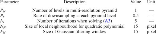
A.2. Validation
The authors would like to underline the difficulties related to conducting meaningful and reliable validation tests. For highly unsteady breaking bores, the strong turbulence with high void fractions limits the alternative instrumentations to measure the flow characteristics on the free surface. Numerically, the DNS modelling is still limited because of the high Reynolds numbers ( ${\approx }10^{6}$). Herein, the instantaneous longitudinal component of the velocity was extracted from the OF data at the roller toe perimeter and used for the validation. The OF data were compared with the experimental bore front celerity data by Wüthrich et al. (Reference Wüthrich, Shi and Chanson2020a), who generated breaking bores with the same flow conditions and experimental facility as the present study. In addition, Wüthrich et al. (Reference Wüthrich, Shi and Chanson2020a) also captured the bore celerity front using several acoustic displacement meters (ADMs), and calculated the longitudinal bore front celerity as the ratio between the separation distance of ADMs and the travel time. The comparison of the longitudinal front velocities with the celerity is presented in figure 25, including (a) the mean bore front celerity and (b) the statistical distribution of the instantaneous bore front celerity. A good agreement was seen for the comparison with the mean bore celerity. For the statistical distribution of the instantaneous bore front celerity, the present dataset was obtained from 22 000 frames, whereas Wüthrich et al. (Reference Wüthrich, Shi and Chanson2020a) calculated it based upon the displacement between consecutive frames ( $U_x = {\rm \Delta} x/ {\rm \Delta} t$, where ${\rm \Delta} t = 1/1000$ f.p.s.) from 25 high-speed videos. Despite this difference, both statistical distributions exhibited right-skewed shape, with similar mean and median values (figure 25b). Overall, these validation tests demonstrated the suitability of the OF technique to compute surface velocities in breaking bores, thus strengthening the validity of these results.

Figure 25. Comparison of the longitudinal bore front celerity data obtained by Wüthrich et al. (Reference Wüthrich, Shi and Chanson2020a) and the present OF results: (a) mean bore front celerity and (b) statistical distribution of the instantaneous bore front celerity.
Appendix B. Synchronisation
The unsteadiness of the breaking bore represented a challenge for the computation of meaningful ensemble statistics. Herein, a novel synchronisation technique was introduced to obtain average velocity field and turbulence statistics. This technique relied on the synchronisation of frames from different videos, based on the longitudinal position of the mean roller toe perimeter, where the transverse profile of the roller toe was identified using the edge detection algorithm proposed by Wüthrich et al. (Reference Wüthrich, Shi and Chanson2020a). An example is provided in figure 26 for a top-view video, in which the bore propagated from the bottom edge to the top edge, opposite to the initial flow direction. The first step was detecting the reference frame where the mean roller toe perimeter was located at one-third of the image plane, from the bottom edge (figure 26a). Then, the roller toes of the following frames were shifted by the difference between their mean roller toe perimeters and the mean roller toe perimeter of the reference frame. The last synchronised frame was taken for the last video frame in which the roller toe perimeter could be fully tracked (figure 26c), i.e. before the bore front left the measuring window. This synchronisation technique allowed ensemble statistical analysis to be carried out based on a different number of samples (frames), depending on the relative location behind the roller toe. This implied that the number of frames had to be large enough to overcome the biases induced by the different number of samples. For this, a minimum number of 22 000 frames was adopted, based on the validation process described in Appendix A.2.

Figure 26. Example of synchronisation process for different top-view video frames: (a) first analysed frame; (b)  $n$th frame between first and last frame; and (c) last analysed frame.


 Open access