


1. Introduction
Aquatic animals school for many reasons from protection against predators and enhanced foraging to increased socialisation and saving energy while swimming (Weihs Reference Weihs1973; Marras et al. Reference Marras, Killen, Lindström, McKenzie, Steffensen and Domenici2015; Ashraf et al. Reference Ashraf, Bradshaw, Ha, Halloy, Godoy-Diana and Thiria2017; Li et al. Reference Li, Nagy, Graving, Bak-Coleman, Xie and Couzin2020). In fact, this energy saving, derived from the hydrodynamic interactions that occur in schools, has been confirmed through direct energy measurements of live fish (Zhang & Lauder Reference Zhang and Lauder2023, Reference Zhang and Lauder2024). These energy benefits can be observed not just among fish in a school, but also between oscillating foils and fish (Harvey et al. Reference Harvey, Muhawenimana, Müller, Wilson and Denissenko2022; Thandiackal & Lauder Reference Thandiackal and Lauder2023) and among oscillating foils (Ristroph & Zhang Reference Ristroph and Zhang2008; Lin et al. Reference Lin, Wu, Zhang and Yang2019; Kurt et al. Reference Kurt, Eslam Panah and Moored2020, Reference Kurt, Mivehchi and Moored2021; Lagopoulos et al. Reference Lagopoulos, Weymouth and Ganapathisubramani2020; Lin et al. Reference Lin, Wu, Yang and Dong2022), which supports the idea that schooling hydrofoils can serve as a simple model of schooling fish and can also be used to propel high-performance underwater biorobots.
In-line formations are canonical schooling arrangements where swimmers are aligned in a leader–follower pattern with followers directly downstream of a leader. Most previous research on in-line schooling has focused on so-called ‘constrained’ or ‘tethered’ foils that have fixed relative spacings. In-line formations of constrained foils show some of the largest hydrodynamic benefits of schooling, where collective thrust and efficiency enhancements have been measured of more than 50 % as compared with an isolated swimmer (Akhtar et al. Reference Akhtar, Mittal, Lauder and Drucker2007; Ristroph & Zhang Reference Ristroph and Zhang2008; Boschitsch et al. Reference Boschitsch, Dewey and Smits2014; Muscutt et al. Reference Muscutt, Weymouth and Ganapathisubramani2017; Kurt & Moored Reference Kurt and Moored2018; Alaminos-Quesada & Fernandez-Feria 2020; Wang et al. Reference Wang, Ng, Teo, Lua and Bao2021; Arranz et al. Reference Arranz, Flores and Garcia-Villalba2022; Han et al. Reference Han, Mivehchi, Kurt and Moored2022a ; Baddoo et al. Reference Baddoo, Moore, Oza and Crowdy2023). These hydrodynamic benefits arise when the wake vortices shed from a leader constructively interact with the leading-edge suction of a follower, and thereby increase its thrust, primarily driven by a modification of its instantaneous angle of attack from the impinging vortices (Akhtar et al. Reference Akhtar, Mittal, Lauder and Drucker2007; Boschitsch et al. Reference Boschitsch, Dewey and Smits2014; Muscutt et al. Reference Muscutt, Weymouth and Ganapathisubramani2017). When a leader’s wake vortex impinges on a follower it also induces the formation of a leading-edge vortex that pairs with the impinging vortex to form either a coherent or a branched wake mode where thrust is maximised or power consumption is minimised, respectively (Boschitsch et al. Reference Boschitsch, Dewey and Smits2014; Kurt & Moored Reference Kurt and Moored2018). Additionally, band structures of high follower efficiency (Boschitsch et al. Reference Boschitsch, Dewey and Smits2014; Kurt & Moored Reference Kurt and Moored2018) reveal that the optimal phase difference or synchrony between a leader and follower follows a linear relationship with their streamwise spacing, which arises from the optimal synchronisation of the follower’s motion to the impinging vortex. While the collective performance is mostly driven by the followers’ performance, in a compact formation a follower can also have a significant upstream influence and enhance a leader’s added mass thrust by providing a blockage effect (Saadat et al. Reference Saadat, Berlinger, Sheshmani, Nagpal, Lauder and Haj-Hariri2021; Pan & Dong Reference Pan and Dong2022; Kelly et al. Reference Kelly, Pan, Menzer and Dong2023). Therefore, the optimal collective efficiency is achieved for relative spacings of less than one chord, and with a properly tuned phase synchrony for a given spacing.
While constrained foil studies provide essential understanding of schooling mechanisms and their potential benefits, their foils are mostly in out-of-equilibrium conditions, meaning that there are thrust imbalances among them that if they were freely swimming, as in real schools, would cause their relative spacing to change and in turn alter their hydrodynamic interactions and benefits. Studies of unconstrained in-line foils able to freely swim in the streamwise direction have shown that streamwise stable spacings arise from their hydrodynamic interactions alone (Becker et al. Reference Becker, Masoud, Newbolt, Shelley and Ristroph2015; Newbolt et al. Reference Newbolt, Zhang and Ristroph2019; Heydari & Kanso Reference Heydari and Kanso2021; Newbolt et al. Reference Newbolt, Lewis, Bleu, Wu, Mavroyiakoumou, Ramananarivo and Ristroph2024). These fluid-mediated formations have a gap distance between foils that is nearly constant, indicating that there is thrust balancing between them, and they are stable since small perturbations from these formations will cause the foils to return to them. These stable spacings were discovered to vary linearly with the phase difference between swimmers leading to multiple stable spacings at the same foil synchronisation that are one wake wavelength apart (Becker et al. Reference Becker, Masoud, Newbolt, Shelley and Ristroph2015; Ramananarivo et al. Reference Ramananarivo, Fang, Oza, Zhang and Ristroph2016; Lin et al. Reference Lin, Wu, Zhang and Yang2019; Newbolt et al. Reference Newbolt, Zhang and Ristroph2019).
Unconstrained studies have examined the enhancement in swimming speed of foils in stable in-line formations (Lin et al. Reference Lin, Wu, Zhang and Yang2019; Newbolt et al. Reference Newbolt, Zhang and Ristroph2019, Reference Newbolt, Zhang and Ristroph2022; Ryu et al. Reference Ryu, Yang, Park and Sung2020; Arranz et al. Reference Arranz, Flores and Garcia-Villalba2022). Regarding power and efficiency benefits, Heydari & Kanso (Reference Heydari and Kanso2021) have probed the power performance of in-line stable foils, but the phase difference between the foils was not varied, nor was leading-edge separation modelled – a key ingredient for forming the characteristic vortex pair observed in in-line schooling that leads to branched and coherent wake modes (Boschitsch et al. Reference Boschitsch, Dewey and Smits2014; Kurt & Moored Reference Kurt and Moored2018). Lin et al. (Reference Lin, Wu, Zhang and Yang2019), Ryu et al. (Reference Ryu, Yang, Park and Sung2020) and Arranz et al. (Reference Arranz, Flores and Garcia-Villalba2022) examined the effect of phase synchrony and revealed the power and efficiency benefits of in-line stable foils at different phase synchronies. However, these studies did not vary the drag loading (represented by the Lighthill number) or the amplitude of the foils. Therefore, the effects of drag loading and amplitude on the power and efficiency benefits of in-line stable foils remain largely unknown. Additionally, considering that unconstrained foil studies show that stable formations occur when the leader and follower are thrust-balanced, we can hypothesise that the power and efficiency benefits of stable formations would be small, unless they are compact, due to constrained foil performance maps showing small power benefits for non-compact spacings when foils are thrust-balanced (Boschitsch et al. Reference Boschitsch, Dewey and Smits2014; Kurt & Moored Reference Kurt and Moored2018). However, constrained foil studies (Kurt et al. Reference Kurt, Mivehchi and Moored2021) have discovered that mismatched amplitudes between a leader and follower foil can enhance the power and efficiency performance of the collective, and unconstrained studies (Newbolt et al. Reference Newbolt, Zhang and Ristroph2019) have shown that in-line foils using mismatched amplitudes can also achieve stable formations. So, can unconstrained in-line foils achieve both high efficiency benefits and a stable formation by using mismatched amplitudes of motion?
To answer this question and provide a comprehensive investigation into the efficiency benefits of in-line schooling, new unconstrained simulations and constrained experiments of a pair of pitching foils in an in-line arrangement are conducted. Using this simple model of a school, we advance our understanding of the hydrodynamic benefits and stability of schooling formations, and their underlying mechanisms, in several ways. While using matched amplitudes of motion, we detail the mechanics of stable in-line formations, and their associated efficiency benefits, for a wide range of flow conditions defined by the Lighthill number and pitching amplitude. We show that the generation of stable formations of pitching foils relies on leading-edge separation. We derive a scaling law for the wake wavelength, $\lambda$
, and demonstrate that the gap distance of stable formations and efficiency performance scales with it, rather than the nominal wake wavelength,
$\lambda$
, and demonstrate that the gap distance of stable formations and efficiency performance scales with it, rather than the nominal wake wavelength, $\lambda _0 = U/f$
(defined more below), used in previous studies (Becker et al. Reference Becker, Masoud, Newbolt, Shelley and Ristroph2015; Ramananarivo et al. Reference Ramananarivo, Fang, Oza, Zhang and Ristroph2016; Newbolt et al. Reference Newbolt, Zhang and Ristroph2019; Heydari & Kanso Reference Heydari and Kanso2021; Newbolt et al. Reference Newbolt, Zhang and Ristroph2022). Additionally, mismatched amplitudes of motion are discovered to substantially enhance the efficiency of stable in-line formations in both simulations and experiments.
$\lambda _0 = U/f$
(defined more below), used in previous studies (Becker et al. Reference Becker, Masoud, Newbolt, Shelley and Ristroph2015; Ramananarivo et al. Reference Ramananarivo, Fang, Oza, Zhang and Ristroph2016; Newbolt et al. Reference Newbolt, Zhang and Ristroph2019; Heydari & Kanso Reference Heydari and Kanso2021; Newbolt et al. Reference Newbolt, Zhang and Ristroph2022). Additionally, mismatched amplitudes of motion are discovered to substantially enhance the efficiency of stable in-line formations in both simulations and experiments.
The paper is organised as follows. Section 2 describes the methodologies used throughout this study and validation of the simulations. Sections 3.1–3.5 present the matched amplitude simulations and development of the scaling of the wake wavelength. Lastly, § 3.6 presents the mismatched amplitude simulations and experiments.
2. Methods
2.1. Problem formulation
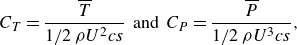
Two foils with a 7 %-thick teardrop-shaped cross-section in an in-line configuration were simulated in two-dimensional potential flow by an in-house advanced boundary element method (ABEM) (see figure 1). Undergoing a pure pitching motion about their leading edges, a pair of leader and follower foils are free to swim in the streamwise ( $X$
) direction, but constrained in the cross-stream (
$X$
) direction, but constrained in the cross-stream ( $Z$
) direction. The gap distance between the leader’s trailing edge and the follower’s leading edge is
$Z$
) direction. The gap distance between the leader’s trailing edge and the follower’s leading edge is $G$
. The properties of the leader and follower are denoted by
$G$
. The properties of the leader and follower are denoted by $(\boldsymbol{\cdot })_{L}$
and
$(\boldsymbol{\cdot })_{L}$
and $(\boldsymbol{\cdot })_{F}$
, respectively. The foils’ kinematics are defined by
$(\boldsymbol{\cdot })_{F}$
, respectively. The foils’ kinematics are defined by
 \begin{align} \theta _{L} = \theta _{0,L}\sin (2\pi ft) \;\; \text{and} \;\; \theta _{F} = \theta _{0,F}\sin (2\pi ft-\phi ), \end{align}
where $\theta$
is the instantaneous pitching angle,
$\theta$
is the instantaneous pitching angle, $\theta _{0}$
is the pitching amplitude,
$\theta _{0}$
is the pitching amplitude, $f$
is the pitching frequency,
$f$
is the pitching frequency, $\phi$
is the phase difference and
$\phi$
is the phase difference and $t$
is time. The pitching angle is considered positive for anticlockwise pitching rotations. The dimensionless amplitude is defined as
$t$
is time. The pitching angle is considered positive for anticlockwise pitching rotations. The dimensionless amplitude is defined as
 \begin{align} A^* = \frac {A}{c}, \end{align}
where $A = 2 c \sin (\theta _0)$
is the peak-to-peak trailing-edge amplitude of the foil, and
$A = 2 c \sin (\theta _0)$
is the peak-to-peak trailing-edge amplitude of the foil, and $c = 0.09$
m is the chord length.
$c = 0.09$
m is the chord length.
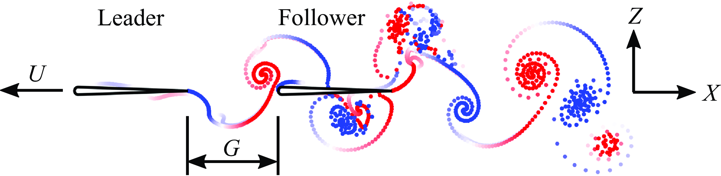
Figure 1. Illustration of hydrofoils pitching in an in-line formation.
The drag force, $D$
, is applied to resist the motion of the foils in the streamwise direction and is used to model the viscous drag generated by the foils and from a virtual body, representing the body of a fish-like swimmer, which is not present in the computational domain (Akoz & Moored Reference Akoz and Moored2018; Ayancik et al. Reference Ayancik, Zhong, Quinn, Brandes, Bart-Smith and Moored2019). Following Akoz et al. (Reference Akoz, Han, Liu, Dong and Moored2019) and Akoz et al. (Reference Akoz, Mivehchi and Moored2021), the drag force is equal to
$D$
, is applied to resist the motion of the foils in the streamwise direction and is used to model the viscous drag generated by the foils and from a virtual body, representing the body of a fish-like swimmer, which is not present in the computational domain (Akoz & Moored Reference Akoz and Moored2018; Ayancik et al. Reference Ayancik, Zhong, Quinn, Brandes, Bart-Smith and Moored2019). Following Akoz et al. (Reference Akoz, Han, Liu, Dong and Moored2019) and Akoz et al. (Reference Akoz, Mivehchi and Moored2021), the drag force is equal to
 \begin{align} D = 1/2 \,\rho u^2 Li \,c s , \end{align}
where $\rho$
is the fluid density,
$\rho$
is the fluid density, $Li$
is the Lighthill number that represents the foil’s drag loading,
$Li$
is the Lighthill number that represents the foil’s drag loading, $s = 1$
m (unit span) is the span length and
$s = 1$
m (unit span) is the span length and $u$
is the swimming speed of the foils. The Lighthill number varies from
$u$
is the swimming speed of the foils. The Lighthill number varies from $0.09$
to
$0.09$
to $0.72$
in this study, which covers a range typical of aquatic animals (Eloy Reference Eloy2013; Akoz & Moored Reference Akoz and Moored2018).
$0.72$
in this study, which covers a range typical of aquatic animals (Eloy Reference Eloy2013; Akoz & Moored Reference Akoz and Moored2018).
The thrust, $T$
, is obtained from the pressure forces acting on the foils projected in the streamwise direction. The instantaneous net thrust,
$T$
, is obtained from the pressure forces acting on the foils projected in the streamwise direction. The instantaneous net thrust, $T_{{net}} = T - D$
, which is the difference between the pressure-based thrust and drag, is used to solve the streamwise equation of motion and to determine the instantaneous swimming speed (see § 2.2.1 for more details). The time-averaged swimming speed,
$T_{{net}} = T - D$
, which is the difference between the pressure-based thrust and drag, is used to solve the streamwise equation of motion and to determine the instantaneous swimming speed (see § 2.2.1 for more details). The time-averaged swimming speed, $U$
, is then defined when the cycle-averaged net thrust is zero, i.e.
$U$
, is then defined when the cycle-averaged net thrust is zero, i.e. $\overline T_{{net}} = 0$
. The time-averaged gap distance,
$\overline T_{{net}} = 0$
. The time-averaged gap distance, $G_s$
, is also averaged after the foils reach a cycle-averaged steady state. The nominal wake wavelength is defined by
$G_s$
, is also averaged after the foils reach a cycle-averaged steady state. The nominal wake wavelength is defined by
 \begin{align} \lambda _{0} = U/f, \end{align}
which has been widely used in previous studies (Becker et al. Reference Becker, Masoud, Newbolt, Shelley and Ristroph2015; Ramananarivo et al. Reference Ramananarivo, Fang, Oza, Zhang and Ristroph2016; Newbolt et al. Reference Newbolt, Zhang and Ristroph2019; Heydari & Kanso Reference Heydari and Kanso2021; Newbolt et al. Reference Newbolt, Zhang and Ristroph2022). Also, the actual wake wavelength, $\lambda$
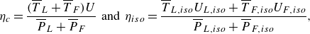
, is measured as the distance between successive vortices of the same sign from the wake of the isolated leader (figure 2
a), which is generally different than, though proportional to, the nominal wavelength. The Strouhal number and reduced frequency are defined by
$\lambda$
, is measured as the distance between successive vortices of the same sign from the wake of the isolated leader (figure 2
a), which is generally different than, though proportional to, the nominal wavelength. The Strouhal number and reduced frequency are defined by
 \begin{align} St = \frac {fA}{U} \;\; \text{and} \;\; k = \frac {fc}{U}, \end{align}
respectively.
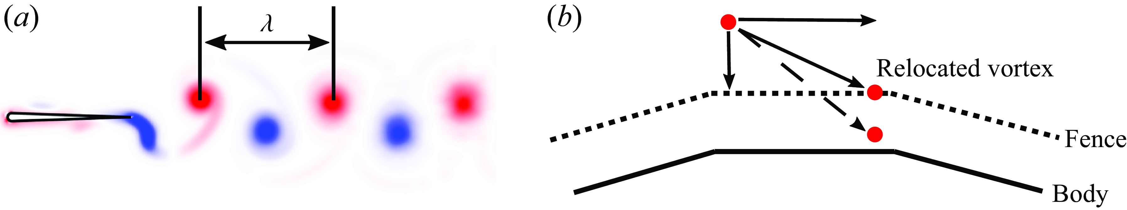
Figure 2. $(a)$
Measurement of the wake wavelength.
$(a)$
Measurement of the wake wavelength. $(b)$
Fencing scheme and wake relocation.
$(b)$
Fencing scheme and wake relocation.
The power input to the fluid, $P$
, is obtained by integrating the inner product between the pressure force vectors and local kinematic velocity vectors along the surface of the foil (defined precisely in § 2.2.1), which is equivalent to the product of the pitching moment about the pitching axis and the angular velocity (Moored & Quinn Reference Moored and Quinn2019). The time-averaged thrust and power coefficients are then defined by
$P$
, is obtained by integrating the inner product between the pressure force vectors and local kinematic velocity vectors along the surface of the foil (defined precisely in § 2.2.1), which is equivalent to the product of the pitching moment about the pitching axis and the angular velocity (Moored & Quinn Reference Moored and Quinn2019). The time-averaged thrust and power coefficients are then defined by
 \begin{align} C_{T} = \frac {\overline {T}}{1/2\, \rho U^2 c s}\;\; \text{and} \;\; C_{P}=\frac {\overline {P}}{1/2\, \rho U^3 c s}, \end{align}
respectively. Following Akoz & Moored (Reference Akoz and Moored2018) and Ayancik et al. (Reference Ayancik, Zhong, Quinn, Brandes, Bart-Smith and Moored2019), the propulsive efficiency is defined based on the thrust of the foil, rather than the net thrust. The collective and isolated efficiency are calculated as
 \begin{align} \eta _{c} = \frac {(\overline {T}_{L}+\overline {T}_{F})U}{\overline {P}_{L}+\overline {P}_{F}} \;\; \text{and} \;\;\eta _{iso} = \frac {\overline {T}_{L,{iso}}U_{L,{iso}}+ \overline {T}_{F,{iso}}U_{F,{iso}}}{\overline {P}_{L,{iso}}+\overline {P}_{F,{iso}}}, \end{align}
respectively. Furthermore, the collective efficiency is normalised by the isolated efficiency to give
 \begin{align} \eta _c^* = \frac {\eta _{c}}{\eta _{iso}}. \end{align}
When the normalised collective efficiency is greater than one, the two schooling foils are more efficient swimming together than in isolation and vice versa.
2.2. Advanced boundary element method
Our in-house potential flow solver is an ABEM that accounts for leading-edge flow separation of the hydrofoils and employs a fencing scheme to prevent wake vortices from penetrating the hydrofoils.
2.2.1. Governing equations
For potential flow that is incompressible, irrotational and inviscid, Laplace’s equation serves as the governing equation,
 \begin{align} \nabla ^2 \Phi ^* \, = \,0. \end{align}
Here $\Phi ^*$
is the perturbation potential in an inertial reference frame fixed to the undisturbed fluid. Additionally, the no-flux boundary condition is satisfied on the two foils’ body surfaces,
$\Phi ^*$
is the perturbation potential in an inertial reference frame fixed to the undisturbed fluid. Additionally, the no-flux boundary condition is satisfied on the two foils’ body surfaces, $S_{b_{L}}$
and
$S_{b_{L}}$
and $S_{b_{F}}$
,
$S_{b_{F}}$
,
 \begin{align} \boldsymbol{n} \boldsymbol{\cdot } \nabla \Phi ^* \, = \, \boldsymbol{n} \boldsymbol{\cdot } (\boldsymbol{u_{rel}} + \boldsymbol{u}), \end{align}
where $\boldsymbol{u_{rel}}$
is the relative velocity to the body-fixed reference frame
$\boldsymbol{u_{rel}}$
is the relative velocity to the body-fixed reference frame $(x,z)$
fixed at a foil’s leading edge, and
$(x,z)$
fixed at a foil’s leading edge, and $\boldsymbol{n}$
is the normal vector pointing outward from the body surface. Additionally, the far-field condition that the flow disturbances caused by the body must decay far away must be satisfied,
$\boldsymbol{n}$
is the normal vector pointing outward from the body surface. Additionally, the far-field condition that the flow disturbances caused by the body must decay far away must be satisfied,
 \begin{align} \underset {|r|\rightarrow \infty }{\text{lim}}( \nabla \Phi ^*)\,=\,0, \end{align}
where $|r|$
is the distance from a target point to the body.
$|r|$
is the distance from a target point to the body.
Following Katz & Plotkin (Reference Katz and Plotkin2001) and Moored (Reference Moored2018), $\Phi ^*$
can be solved by the boundary integral equation that considers a combination of constant-strength sources,
$\Phi ^*$
can be solved by the boundary integral equation that considers a combination of constant-strength sources, $\sigma$
, and doublets,
$\sigma$
, and doublets, $\mu$
, on the body surface and constant-strength doublets,
$\mu$
, on the body surface and constant-strength doublets, $\mu _{w}$
, on the two foils’ wake surfaces,
$\mu _{w}$
, on the two foils’ wake surfaces,
 \begin{gather} \Phi ^*_{i}(r) = \iint \limits_{S_b^*} [\sigma (r_{0})G(r;r_{0}) - \mu (r_{0})\boldsymbol{n}\boldsymbol{\cdot }\nabla G(r;r_{0})] \text{d} S - \iint \limits_{S_w^*} \mu _{w}(r_{0})\boldsymbol{n} \boldsymbol{\cdot } \nabla G(r;r_{0}) \text{d} S \end{gather}
with
 \begin{gather} \sigma = \boldsymbol{n} \boldsymbol{\cdot } \nabla (\Phi ^* - \Phi ^*_{i}) \;\;\text{and} \;\; -\!\mu = \Phi ^* - \Phi ^*_{i}, \end{gather}
where $\Phi ^*_{i}$
is the internal potential,
$\Phi ^*_{i}$
is the internal potential, $S_b^* = S_{b,L} + S_{b,F}$
is the combined body surfaces,
$S_b^* = S_{b,L} + S_{b,F}$
is the combined body surfaces, $S_w^* = S_{w,L} + S_{w,F}$
is the combined wake surfaces,
$S_w^* = S_{w,L} + S_{w,F}$
is the combined wake surfaces, $r_{0}$
is a source or doublet’s location,
$r_{0}$
is a source or doublet’s location, $r$
is the location of the target point and the Green’s function is
$r$
is the location of the target point and the Green’s function is $G(r;r_{0})=(1/2\pi ) \ln | r-r_{0}|$
. The Dirichlet boundary condition is enforced by setting the internal potential to be zero,
$G(r;r_{0})=(1/2\pi ) \ln | r-r_{0}|$
. The Dirichlet boundary condition is enforced by setting the internal potential to be zero, $\Phi ^*_{i}$
= 0, which gives
$\Phi ^*_{i}$
= 0, which gives
 \begin{gather} \sigma = \boldsymbol{n} \boldsymbol{\cdot } \nabla \Phi ^* = \boldsymbol{n} \boldsymbol{\cdot } (\boldsymbol{u_{rel}} + \boldsymbol{u}) \;\; \text{and} \;\; -\!\mu = \Phi ^*. \end{gather}
Consequently, $\sigma$
becomes a known value, and
$\sigma$
becomes a known value, and $\Phi ^*$
can be calculated by solving
$\Phi ^*$
can be calculated by solving $\mu$
over the body. Conveniently, the far-field condition is implicitly satisfied by the source and doublet elements.
$\mu$
over the body. Conveniently, the far-field condition is implicitly satisfied by the source and doublet elements.
Each of the foils’ body surfaces are discretised into $N$
panels. The doublet strength of every body panel is unknown. Also, the wake surfaces of the foils are discretised into doublet panels. At each time step, a trailing edge panel will shed from each foil into the fluid, whose strength will not change in time and a new trailing edge panel will form. The strength of the trailing-edge panel is determined by enforcing the Kutta condition, that is, zero vorticity at the trailing edge,
$N$
panels. The doublet strength of every body panel is unknown. Also, the wake surfaces of the foils are discretised into doublet panels. At each time step, a trailing edge panel will shed from each foil into the fluid, whose strength will not change in time and a new trailing edge panel will form. The strength of the trailing-edge panel is determined by enforcing the Kutta condition, that is, zero vorticity at the trailing edge,
 \begin{align} \mu _{TE} = \mu _{+} - \mu _{-}, \end{align}
where $\mu _{TE}$
is the strength of the trailing-edge panel,
$\mu _{TE}$
is the strength of the trailing-edge panel, $\mu _{+}$
is the doublet strength of the body panel on the upper surface at the trailing edge and
$\mu _{+}$
is the doublet strength of the body panel on the upper surface at the trailing edge and $\mu _{-}$
is the doublet strength of the body panel on the lower surface at the trailing edge. The trailing-edge panel is oriented along a line that bisects the upper and lower surfaces of the body at the trailing edge, whose length is set to
$\mu _{-}$
is the doublet strength of the body panel on the lower surface at the trailing edge. The trailing-edge panel is oriented along a line that bisects the upper and lower surfaces of the body at the trailing edge, whose length is set to $0.4 U \Delta t$
for both numerical stability and computational accuracy, where the simulation time step is
$0.4 U \Delta t$
for both numerical stability and computational accuracy, where the simulation time step is $\Delta t$
. This panel length gives good solution convergence while maintaining solution accuracy with the following validation cases. There are
$\Delta t$
. This panel length gives good solution convergence while maintaining solution accuracy with the following validation cases. There are $2N$
unknowns
$2N$
unknowns $\mu$
, and they can be solved by
$\mu$
, and they can be solved by $2N$
equations (2.12) enforced at
$2N$
equations (2.12) enforced at $2N$
collocation points. These points are located at the centre of panels, but moved inside the body along the surface normal vector by
$2N$
collocation points. These points are located at the centre of panels, but moved inside the body along the surface normal vector by $10\,\%$
of the local body thickness.
$10\,\%$
of the local body thickness.
Then the pressure field over the body, $p$
, can be calculated by the unsteady Bernoulli equation,
$p$
, can be calculated by the unsteady Bernoulli equation,
 \begin{align} p(x,z,t)=-\rho \frac {\partial \Phi ^*}{\partial t} + \rho (\boldsymbol{u}_{\boldsymbol{rel}} + \mathbf{u}) \boldsymbol{\cdot } \nabla \Phi ^* -\rho \frac {(\nabla \Phi ^*)^2}{2}. \end{align}
The thrust, $T$
, and lift,
$T$
, and lift, $L$
, can be calculated by integrating the normal forces from the pressure fields, projected in the
$L$
, can be calculated by integrating the normal forces from the pressure fields, projected in the $x$
and
$x$
and $z$
directions, acting on the body surfaces,
$z$
directions, acting on the body surfaces,
 \begin{align} T = \int _{S_{b}} - p \boldsymbol{n} \boldsymbol{\cdot } \boldsymbol{x} \, \text{d} S \;\; \text{and} \;\; L = \int _{S_{b}} - p \boldsymbol{n} \boldsymbol{\cdot } \boldsymbol{z} \, \text{d} S, \end{align}
where $\boldsymbol{x}$
is the unit vector in the streamwise direction, and
$\boldsymbol{x}$
is the unit vector in the streamwise direction, and $\boldsymbol{z}$
is the unit vector in the cross-stream direction. Power consumption is calculated by
$\boldsymbol{z}$
is the unit vector in the cross-stream direction. Power consumption is calculated by
 \begin{align} P = \int _{S_{b}} - p \boldsymbol{n} \boldsymbol{\cdot } \boldsymbol{u_{rel}} \, \text{d} S. \end{align}
To calculate the foils’ free-swimming motion in the streamwise direction, the velocity and location of the foil at the $(n + 1)$
th time step are calculated by forward differencing (Moored Reference Moored2018; Ayancik et al. Reference Ayancik, Fish and Moored2020),
$(n + 1)$
th time step are calculated by forward differencing (Moored Reference Moored2018; Ayancik et al. Reference Ayancik, Fish and Moored2020),
 \begin{align} u^{n+1} = u^{n} + \frac {T_{net}^{n}}{m} \Delta t \;\; \text{and} \;\; X^{n+1} = X^{n} + \frac {1}{2}(u^{n+1}+u^{n}) \Delta t, \end{align}
where $X$
is the location of a foil’s leading edge in the streamwise direction, and
$X$
is the location of a foil’s leading edge in the streamwise direction, and $m$
is the mass of the foil, which is fixed in this study at three times the characteristic added mass of the foils, i.e.
$m$
is the mass of the foil, which is fixed in this study at three times the characteristic added mass of the foils, i.e. $m = 3\rho s c^2$
.
$m = 3\rho s c^2$
.
The number of body panels per foil and time steps per pitching cycle were both set to $250$
based on convergence studies, which showed that stable formations change by less than
$250$
based on convergence studies, which showed that stable formations change by less than $2\,\%$
when both are doubled from
$2\,\%$
when both are doubled from $250$
to
$250$
to $500$
, independently.
$500$
, independently.
2.2.2. Leading-edge flow separation
Following Ramesh et al. (Reference Ramesh, Gopalarathnam, Granlund, Ol and Edwards2014), a leading-edge separation mechanism is coupled with the potential flow solver based on the leading-edge suction parameter (LESP), which indicates the suction strength at a foil’s leading edge. Based on Narsipur et al. (Reference Narsipur, Hosangadi, Gopalarathnam and Edwards2020), the instantaneous LESP value is calculated by
 \begin{align} \text{LESP}(t) = A_{0}(t) = -\frac {1}{\pi u_{{net}}}\int _{0}^{\pi }\frac {\partial \Phi ^*_{B}}{\partial z} \text{d} \alpha \end{align}
with
 \begin{align} x = \frac {c}{2}(1-\cos {\alpha }) \end{align}
and
 \begin{align} u_{{net}}(t) = \sqrt {\left [u(t) + \tfrac {1}{2}\dot {\theta }(t)c\sin {\theta (t)}\right ]^2 + \left [\tfrac {1}{2}\dot {\theta }(t)c\cos {\theta (t)}\right ]}, \end{align}
where $\Phi ^*_{B}$
is the perturbation potential generated by bound vortices,
$\Phi ^*_{B}$
is the perturbation potential generated by bound vortices, $\alpha$
is a transformation variable associated with the chordwise coordinate
$\alpha$
is a transformation variable associated with the chordwise coordinate $x$
and the direction normal to a foil’s chord line is
$x$
and the direction normal to a foil’s chord line is $z$
. According to Ramesh et al. (Reference Ramesh, Gopalarathnam, Granlund, Ol and Edwards2014), a leading-edge vortex will be shed when
$z$
. According to Ramesh et al. (Reference Ramesh, Gopalarathnam, Granlund, Ol and Edwards2014), a leading-edge vortex will be shed when $|\text{LESP}|$
exceeds its critical value
$|\text{LESP}|$
exceeds its critical value $\text{LESP}_{{crit}}$
, and, by shedding a leading edge vortex element,
$\text{LESP}_{{crit}}$
, and, by shedding a leading edge vortex element, $|\text{LESP}|$
will be brought back to its critical value,
$|\text{LESP}|$
will be brought back to its critical value,
 \begin{align} |\text{LESP}(t)| = \text{LESP}_{{crit}}. \end{align}
Additionally, $\text{LESP}_{{crit}}$
depends on the foil’s shape and Reynolds number.
$\text{LESP}_{{crit}}$
depends on the foil’s shape and Reynolds number.
At each time step, $2N$
equations (2.12) are solved without shedding any leading-edge vortices first, then
$2N$
equations (2.12) are solved without shedding any leading-edge vortices first, then $\text{LESP}$
is calculated. If the
$\text{LESP}$
is calculated. If the $|\text{LESP}|$
of the foils does not exceed their critical values then the simulation moves to the next time step. If the
$|\text{LESP}|$
of the foils does not exceed their critical values then the simulation moves to the next time step. If the $|\text{LESP}|$
of the foils exceed their critical values, an additional (2.23) will be formulated for and an additional unknown leading-edge vortex will be shed from each foil exceeding its critical value.
$|\text{LESP}|$
of the foils exceed their critical values, an additional (2.23) will be formulated for and an additional unknown leading-edge vortex will be shed from each foil exceeding its critical value.
2.2.3. Wake–body interaction
To represent the advection of vorticity with the local flow velocity a so-called ‘wake roll-up’ or wake element advection scheme must be applied at every time step. To calculate the induced flow velocity from the wake elements on themselves, the elements must be desingularised for numerical stability. Following previous work (Vatistas et al. Reference Vatistas, Kozel and Mih1991; Ramesh et al. Reference Ramesh, Gopalarathnam, Granlund, Ol and Edwards2014; Sedky et al. Reference Sedky, Lagor and Jones2020), the induced velocity of a constant strength doublet element is equivalent to two counter-rotating point vortices located at the element end points, which can be calculated using the desingularised Lamb–Oseen two-dimensional vortex model,
 \begin{align} \boldsymbol{u}_{i}(\boldsymbol{r}) = \frac {\Gamma _{i}}{2\pi }\frac {{\boldsymbol{y}\times (\boldsymbol{r}-\boldsymbol{r_{i}})}}{\sqrt {|\boldsymbol{r}-\boldsymbol{r_{i}}|^4 + \delta ^4}} \;\; \text{and} \;\; \boldsymbol{r}-\boldsymbol{r_{i}} = (x-x_{i})\boldsymbol{x}+ (z-z_{i})\boldsymbol{z}. \end{align}
Here $(x,z)$
is the coordinate of the influence point,
$(x,z)$
is the coordinate of the influence point, $(x_{i},z_{i})$
is the coordinate of the
$(x_{i},z_{i})$
is the coordinate of the $i$
th vortex,
$i$
th vortex, $\Gamma _{i}$
is the strength of the
$\Gamma _{i}$
is the strength of the $i$
th vortex and
$i$
th vortex and $\delta$
is the desingularisation parameter. The desingularisation parameter is a free parameter and is used to mimic the effect of viscosity in real fluids by giving each point vortex a core radius. We choose the lowest value for
$\delta$
is the desingularisation parameter. The desingularisation parameter is a free parameter and is used to mimic the effect of viscosity in real fluids by giving each point vortex a core radius. We choose the lowest value for $\delta$
that prevents numerical instability during wake advection. It increases from
$\delta$
that prevents numerical instability during wake advection. It increases from $\delta = 0.06$
to
$\delta = 0.06$
to $0.25$
when the pitching amplitude increases from
$0.25$
when the pitching amplitude increases from $\theta _0 = 7.5^{\circ }$
to
$\theta _0 = 7.5^{\circ }$
to $30^{\circ }$
.
$30^{\circ }$
.
In order to prevent wake vortex elements from penetrating the foils during advection, a fence with thickness of 3 % of the chord length is built around each foil, following the convergence study in Pan et al. (Reference Pan, Dong, Zhu and Yue2012). When a vortex penetrates the body a fencing scheme is applied and it is relocated such that the displacement of the element end point normal to the surface is cancelled while the displacement tangent to the surface is preserved (figure 2 b).
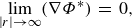
2.3. Experimental set-up
To identify potential efficiency benefits for unconstrained foils and to verify the mismatched amplitude simulation results, we conducted experiments on two constrained foils in in-line arrangements undergoing the same kinematics as the unconstrained foils. Measurements occurred in a closed-loop water tunnel (figure 3) with a splitter and surface plate used to create a nominally two-dimensional flow. Two identical hydrofoils, designated as the leader and follower, were used and had a rectangular planform shape, a chord length of $c = 0.09$
m, a span length of
$c = 0.09$
m, a span length of $s = 0.18$
m, giving them an aspect ratio of two. The foils were made of acrylonitrile butadiene styrene and featured the same cross-sectional shape as foils in the simulations. The pitching kinematics of the foils were controlled by Dynamixel MX-64T servomotors and the pitching axis was set at the leading edge of the foils. Details of the kinematics of the foils can be found in § 2.1. The phase difference of the foils varies between
$s = 0.18$
m, giving them an aspect ratio of two. The foils were made of acrylonitrile butadiene styrene and featured the same cross-sectional shape as foils in the simulations. The pitching kinematics of the foils were controlled by Dynamixel MX-64T servomotors and the pitching axis was set at the leading edge of the foils. Details of the kinematics of the foils can be found in § 2.1. The phase difference of the foils varies between $0\leqslant \phi \leqslant 2\pi$
with increments of
$0\leqslant \phi \leqslant 2\pi$
with increments of $\pi /4$
, producing eight different phase synchronies for each arrangement. The gap distance was varied between
$\pi /4$
, producing eight different phase synchronies for each arrangement. The gap distance was varied between $0.25c \leqslant G \leqslant 1.75c$
with increments of
$0.25c \leqslant G \leqslant 1.75c$
with increments of $0.25c$
by utilising an automated traverse mechanism. The pitching frequency and amplitude, phase difference and flow speed of the constrained experiments were kept consistent with those of the unconstrained simulations. Two ATI Mini-40E six-axis force sensors were used on both leader and follower foils to measure the thrust and pitching moment acting on each foil. Further details of the force measurement set-up can be found in Kurt & Moored (Reference Kurt and Moored2018) and Han et al. (Reference Han, Pan, Liu and Dong2022b
). During each trial the thrust and power were time-averaged over
$0.25c$
by utilising an automated traverse mechanism. The pitching frequency and amplitude, phase difference and flow speed of the constrained experiments were kept consistent with those of the unconstrained simulations. Two ATI Mini-40E six-axis force sensors were used on both leader and follower foils to measure the thrust and pitching moment acting on each foil. Further details of the force measurement set-up can be found in Kurt & Moored (Reference Kurt and Moored2018) and Han et al. (Reference Han, Pan, Liu and Dong2022b
). During each trial the thrust and power were time-averaged over $60$
pitching cycles and these mean values are averaged over five trials and reported. Collective and isolated efficiencies are calculated following (2.7). The maximum standard deviation of the five trials for the measured efficiencies is
$60$
pitching cycles and these mean values are averaged over five trials and reported. Collective and isolated efficiencies are calculated following (2.7). The maximum standard deviation of the five trials for the measured efficiencies is $2.5\,\%$
.
$2.5\,\%$
.
Figure 3. Schematic of experimental set-up.
2.4. Numerical validation
In order to validate the in-house ABEM solver three validation cases are presented, which cover a foil performing a pitch manoeuvre, a foil in combined heaving and pitching motion, and two foils in an in-line schooling formation.
2.4.1. Pitch manoeuvre
Figure 4 present the forces and flow structures simulated with the ABEM solver compared with previous computational fluid dynamics (CFD) results from a viscous vortex particle method (Wang & Eldredge Reference Wang and Eldredge2013). A $2.3\,\%$
-thick flat plate pitching about its leading edge was simulated at
$2.3\,\%$
-thick flat plate pitching about its leading edge was simulated at $ Re = 1000$
. The critical LESP was chosen to be
$ Re = 1000$
. The critical LESP was chosen to be $\text{LESP}_{{crit}} = 0.1$
(Ramesh et al. Reference Ramesh, Gopalarathnam, Granlund, Ol and Edwards2014). The instantaneous pitch angle of the foil was given by
$\text{LESP}_{{crit}} = 0.1$
(Ramesh et al. Reference Ramesh, Gopalarathnam, Granlund, Ol and Edwards2014). The instantaneous pitch angle of the foil was given by
 \begin{align} \theta (t^*) = \theta _{0} \frac {G}{G_{{max}}}, \end{align}
with
 \begin{align} G(t^*) = \log \left \{ \frac {\cosh {\left [a_s(t^*-t_{1}^*)\right ]}}{\cosh {\left [a_s(t^*-t_{2}^*)\right ]}} \right \} - a_s(t_{1}^*-t_{2}^*), \end{align}
where $a_s = 11$
is the smoothing parameter,
$a_s = 11$
is the smoothing parameter, $t^*$
is the dimensionless time with
$t^*$
is the dimensionless time with $t^* = tU_{\infty }/c$
and
$t^* = tU_{\infty }/c$
and $U_{\infty }/c = 1$
,
$U_{\infty }/c = 1$
, $t_{1}^*$
and
$t_{1}^*$
and $t_{2}^*$
are two constants with
$t_{2}^*$
are two constants with $t_{1}^* = 1$
and
$t_{1}^* = 1$
and $t_{2}^* = 1 + 5\pi /4$
, and
$t_{2}^* = 1 + 5\pi /4$
, and $G_{{max}}$
is the maximum of
$G_{{max}}$
is the maximum of $G$
when
$G$
when $t^*$
varies from
$t^*$
varies from $0$
to
$0$
to $5$
. In figure 4, it is found that both force data and flow structures are in good agreement with the CFD results.
$5$
. In figure 4, it is found that both force data and flow structures are in good agreement with the CFD results.
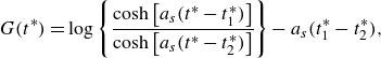
Figure 4. The ABEM potential flow solver shows good agreement with CFD results calculated using a viscous vortex particle method (Wang & Eldredge Reference Wang and Eldredge2013) for a pitch manoeuvre. The forces are compared in $(a)$
for the drag coefficient and in
$(a)$
for the drag coefficient and in $(b)$
for the lift coefficient. The flow structures are compared in
$(b)$
for the lift coefficient. The flow structures are compared in $(c)$
and
$(c)$
and $(d)$
at different times. Normalised vorticity,
$(d)$
at different times. Normalised vorticity, $\omega ^{*}$
, is calculated as
$\omega ^{*}$
, is calculated as $\omega ^{*} = \omega c/U$
.
$\omega ^{*} = \omega c/U$
.
2.4.2. Combined heaving and pitching
Figure 5 presents ABEM simulation data compared with previous experiments (Read et al. Reference Read, Hover and Triantafyllou2003) of a NACA $0012$
hydrofoil performing combined heaving and pitching motion at
$0012$
hydrofoil performing combined heaving and pitching motion at $Re = 40\,000$
. The foil’s kinematics are given as
$Re = 40\,000$
. The foil’s kinematics are given as
 \begin{align} h(t) = h_{0}\sin {(2\pi f t)} \;\; \text{and} \;\; \theta (t) = \theta _{0}\sin {(2\pi f t + \pi /2)}, \end{align}
where $h(t)$
is the foil’s heaving motion, and the foil’s heaving amplitude,
$h(t)$
is the foil’s heaving motion, and the foil’s heaving amplitude, $h_{0}$
, is fixed at one chord length with
$h_{0}$
, is fixed at one chord length with $c = 0.1\,\text{m}$
. The instantaneous angle of attack of the foil is calculated by
$c = 0.1\,\text{m}$
. The instantaneous angle of attack of the foil is calculated by
 \begin{align} \alpha (t) = \theta (t) - \tan ^{-1} \left [\frac {\dot {h}(t)}{U_{\infty }}\right ]. \end{align}
The free stream velocity is $U_\infty = 0.4\,\text{m}{\rm s^-{^1}}$
. The maximum angle of attack,
$U_\infty = 0.4\,\text{m}{\rm s^-{^1}}$
. The maximum angle of attack, $\alpha _{{max}}$
, is the maximum
$\alpha _{{max}}$
, is the maximum $\alpha$
within one cycle of oscillation, and simulations were conducted at two maximum angles of attack that were
$\alpha$
within one cycle of oscillation, and simulations were conducted at two maximum angles of attack that were $\alpha _{{max}} = 15^{\circ }$
and
$\alpha _{{max}} = 15^{\circ }$
and $40^{\circ }$
. Narsipur et al. (Reference Narsipur, Hosangadi, Gopalarathnam and Edwards2020) showed that
$40^{\circ }$
. Narsipur et al. (Reference Narsipur, Hosangadi, Gopalarathnam and Edwards2020) showed that $\text{LESP}_{{crit}}$
varies when the non-dimensional rate of change of angle of attack,
$\text{LESP}_{{crit}}$
varies when the non-dimensional rate of change of angle of attack, $K = \dot {\alpha }c/2U_{\infty }$
, has a large variation, which happens in the combined pitching and heaving motion. According to Narsipur et al. (Reference Narsipur, Hosangadi, Gopalarathnam and Edwards2020),
$K = \dot {\alpha }c/2U_{\infty }$
, has a large variation, which happens in the combined pitching and heaving motion. According to Narsipur et al. (Reference Narsipur, Hosangadi, Gopalarathnam and Edwards2020), $\text{LESP}_{{crit}}$
increases from
$\text{LESP}_{{crit}}$
increases from $0.15$
to
$0.15$
to $0.2$
based on the average rate of change of angle of attack,
$0.2$
based on the average rate of change of angle of attack, $K_{\text{avg}} = 2\alpha _{{max}}cf/U_{\infty }$
. Figure 5 presents the comparison of thrust and efficiency at the two maximum angles of attack between the ABEM simulations and experiments. It shows that the ABEM simulations are in good agreement with the experimental data. In addition, it is discovered that thrust and efficiency are significantly overpredicted when there is no leading-edge separation model and
$K_{\text{avg}} = 2\alpha _{{max}}cf/U_{\infty }$
. Figure 5 presents the comparison of thrust and efficiency at the two maximum angles of attack between the ABEM simulations and experiments. It shows that the ABEM simulations are in good agreement with the experimental data. In addition, it is discovered that thrust and efficiency are significantly overpredicted when there is no leading-edge separation model and $\alpha _{{max}}=40^{\circ }$
.
$\alpha _{{max}}=40^{\circ }$
.
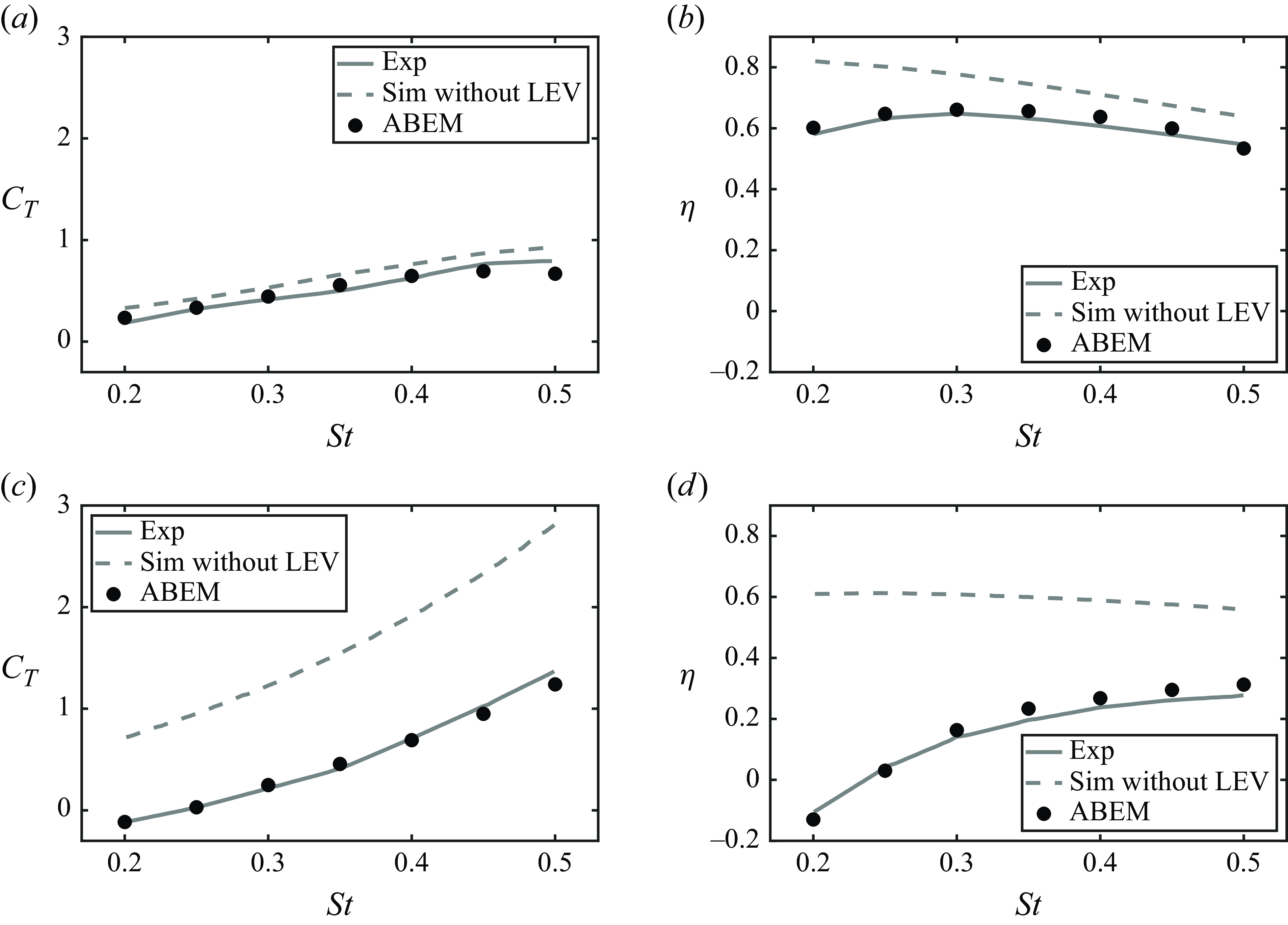
Figure 5. Validation of a hydrofoil performing combined heaving and pitching motion. The $(a)$
thrust coefficient and
$(a)$
thrust coefficient and $(b)$
efficiency at
$(b)$
efficiency at $\alpha _{{max}}=15^{\circ }$
. The
$\alpha _{{max}}=15^{\circ }$
. The $(c)$
thrust coefficient and
$(c)$
thrust coefficient and $(d)$
efficiency at
$(d)$
efficiency at $\alpha _{{max}}=40^{\circ }$
. The ABEM simulation data with and without a leading-edge vortices (LEV) shedding are represented by black circles and dashed lines, respectively. Experimental data from Read et al. (Reference Read, Hover and Triantafyllou2003) is represented by solid lines.
$\alpha _{{max}}=40^{\circ }$
. The ABEM simulation data with and without a leading-edge vortices (LEV) shedding are represented by black circles and dashed lines, respectively. Experimental data from Read et al. (Reference Read, Hover and Triantafyllou2003) is represented by solid lines.
2.4.3. In-line schooling of a pair of pitching foils
Figure 6 presents simulations of constrained pitching foils in an in-line schooling formation. Simulations were conducted for two pitching foils with a 7 %-thick teardrop cross-sectional shape and validated against previous experimental data at a Reynolds number of $7500$
(Kurt & Moored Reference Kurt and Moored2018). The gap distance is fixed at
$7500$
(Kurt & Moored Reference Kurt and Moored2018). The gap distance is fixed at $G/c=0.25$
, and the phase difference varies from
$G/c=0.25$
, and the phase difference varies from $0 \leqslant \phi \leqslant 7\pi /4$
. The foils’ pitching frequency and amplitude are fixed at
$0 \leqslant \phi \leqslant 7\pi /4$
. The foils’ pitching frequency and amplitude are fixed at $f = 0.75$
Hz and
$f = 0.75$
Hz and $\theta _0 = 7.5^{\circ }$
, respectively. In addition, the foils’ chord length is fixed at
$\theta _0 = 7.5^{\circ }$
, respectively. In addition, the foils’ chord length is fixed at $c = 0.09$
m, and the free stream velocity is fixed at
$c = 0.09$
m, and the free stream velocity is fixed at $U_\infty = 0.071\,\rm ms^-{^1}$
. According to Ramesh et al. (Reference Ramesh, Gopalarathnam, Granlund, Ol and Edwards2014),
$U_\infty = 0.071\,\rm ms^-{^1}$
. According to Ramesh et al. (Reference Ramesh, Gopalarathnam, Granlund, Ol and Edwards2014), $\text{LESP}_{{crit}} = 0.1$
was determined by finding the value that can provide the best match with the experimental thrust data of an isolated foil. Additionally, this
$\text{LESP}_{{crit}} = 0.1$
was determined by finding the value that can provide the best match with the experimental thrust data of an isolated foil. Additionally, this $\text{LESP}_{{crit}}$
is fixed for simulations in this article. Although the simulations are in potential flow, the leading-edge vortex shedding is for the Reynolds number of
$\text{LESP}_{{crit}}$
is fixed for simulations in this article. Although the simulations are in potential flow, the leading-edge vortex shedding is for the Reynolds number of $7500$
. The normalised time-averaged thrust and power coefficients of the leader are defined by
$7500$
. The normalised time-averaged thrust and power coefficients of the leader are defined by
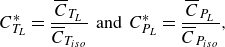 \begin{align} C_{T_L}^* = \frac {\overline {C}_{T_{L}}}{\overline {C}_{T_{{iso}}}} \;\; \text{and} \;\; C_{P_L}^* = \frac {\overline {C}_{P_{L}}}{\overline {C}_{P_{{iso}}}}, \end{align}
respectively, where $\overline {C}_{T_{\textit{iso}}}$
and
$\overline {C}_{T_{\textit{iso}}}$
and $\overline {C}_{P_{\textit{iso}}}$
are the time-averaged thrust and power coefficients of an isolated foil, respectively. Similarly, the normalised time-averaged thrust and power coefficients of the follower can be defined. Figure 6(a–d) shows a good agreement in the normalised thrust and power coefficients between ABEM simulations and experiments across the full range of phase difference. Figures 6(e) and 6(f) highlight that the ABEM simulations also capture the main vortex structures observed in the particle image velocimetry data further validating the simulations.
$\overline {C}_{P_{\textit{iso}}}$
are the time-averaged thrust and power coefficients of an isolated foil, respectively. Similarly, the normalised time-averaged thrust and power coefficients of the follower can be defined. Figure 6(a–d) shows a good agreement in the normalised thrust and power coefficients between ABEM simulations and experiments across the full range of phase difference. Figures 6(e) and 6(f) highlight that the ABEM simulations also capture the main vortex structures observed in the particle image velocimetry data further validating the simulations.
Figure 6. Validation of in-line schooling simulations against previous experimental data (Kurt & Moored Reference Kurt and Moored2018). Normalised thrust coefficient for $(a)$
the leader foil and
$(a)$
the leader foil and $(c)$
the follower foil. Normalised power coefficient for
$(c)$
the follower foil. Normalised power coefficient for $(b)$
the leader foil and
$(b)$
the leader foil and $(d)$
the follower foil. Error bars represent plus or minus one standard deviation. Comparison of vorticity between (i) the experiments and (ii) simulations for
$(d)$
the follower foil. Error bars represent plus or minus one standard deviation. Comparison of vorticity between (i) the experiments and (ii) simulations for $\phi = \pi /4$
at
$\phi = \pi /4$
at $(e)$
$(e)$ $t/T = 0$
and
$t/T = 0$
and $(f)$
$(f)$ $t/T = 0.5$
.
$t/T = 0.5$
.
3. Results
Sections 3.1–3.4 present results from simulations of two streamwise unconstrained pitching hydrofoils swimming in an in-line formation over a wide range of Lighthill number, matched pitching amplitude and phase difference. In addition, simulations with and without leading-edge flow separation were conducted to probe its effect on the formation of in-line stable arrangements. Suppressing leading-edge flow separation was achieved by giving $\text{LESP}_{{crit}}$
an effectively infinite value (chosen to be 100 in this study). The input variables used in these sections are detailed in table 1. Section 3.6 presents constrained experiments and unconstrained simulations of mismatched amplitudes where the leader has a larger amplitude than the follower. The input variables for this section are also detailed in table 1.
$\text{LESP}_{{crit}}$
an effectively infinite value (chosen to be 100 in this study). The input variables used in these sections are detailed in table 1. Section 3.6 presents constrained experiments and unconstrained simulations of mismatched amplitudes where the leader has a larger amplitude than the follower. The input variables for this section are also detailed in table 1.
Table 1. Input parameters and variables used in the current study.
3.1. Varying the condition of leading-edge flow separation
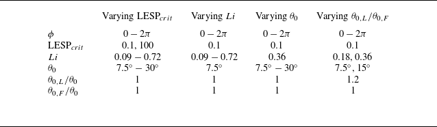
A representative simulation case with and without leading-edge flow separation is presented in figure 7, where $Li = 0.36$
,
$Li = 0.36$
, $ \theta _{0} = 7.5^{\circ }$
and
$ \theta _{0} = 7.5^{\circ }$
and $\phi =\pi$
. Figure 7(a) shows that the leader and follower foils’ wide range of initial gap distances evolve to settle into three distinct stable gap distances when leading-edge flow separation is present, as observed previously in experiments (Becker et al. Reference Becker, Masoud, Newbolt, Shelley and Ristroph2015; Ramananarivo et al. Reference Ramananarivo, Fang, Oza, Zhang and Ristroph2016; Newbolt et al. Reference Newbolt, Zhang and Ristroph2019). However, figure 7(b) shows that when leading-edge separation is suppressed the follower always collides with the leader (
$\phi =\pi$
. Figure 7(a) shows that the leader and follower foils’ wide range of initial gap distances evolve to settle into three distinct stable gap distances when leading-edge flow separation is present, as observed previously in experiments (Becker et al. Reference Becker, Masoud, Newbolt, Shelley and Ristroph2015; Ramananarivo et al. Reference Ramananarivo, Fang, Oza, Zhang and Ristroph2016; Newbolt et al. Reference Newbolt, Zhang and Ristroph2019). However, figure 7(b) shows that when leading-edge separation is suppressed the follower always collides with the leader ( $G/c \rightarrow 0$
) regardless of its initial gap distance. Furthermore, this phenomenon occurs across the whole range of Lighthill number, pitching amplitude and phase difference shown in table 1 (varying
$G/c \rightarrow 0$
) regardless of its initial gap distance. Furthermore, this phenomenon occurs across the whole range of Lighthill number, pitching amplitude and phase difference shown in table 1 (varying $\text{LESP}_{{crit}}$
). Figures 7(c) and 7(d) show that the characteristic vortex pairs that form on the top and bottom of the follower experiencing in-line interactions (Boschitsch et al. Reference Boschitsch, Dewey and Smits2014; Kurt & Moored Reference Kurt and Moored2018) disappear when separation is suppressed.
$\text{LESP}_{{crit}}$
). Figures 7(c) and 7(d) show that the characteristic vortex pairs that form on the top and bottom of the follower experiencing in-line interactions (Boschitsch et al. Reference Boschitsch, Dewey and Smits2014; Kurt & Moored Reference Kurt and Moored2018) disappear when separation is suppressed.
Figure 7. Leading-edge flow separation is critical for generating stable in-line formations. Trajectories for $Li = 0.36$
,
$Li = 0.36$
, $\theta _{0} = 7.5^{\circ }$
and
$\theta _{0} = 7.5^{\circ }$
and $\phi =\pi$
:
$\phi =\pi$
: $(a)$
simulations with leading-edge flow separation,
$(a)$
simulations with leading-edge flow separation, $\text{LESP}_{{crit}}=0.1$
, and
$\text{LESP}_{{crit}}=0.1$
, and $(b)$
simulations without leading-edge flow separation,
$(b)$
simulations without leading-edge flow separation, $\text{LESP}_{{crit}}=100$
. Normalised vorticity,
$\text{LESP}_{{crit}}=100$
. Normalised vorticity, $\omega ^{*} = \omega c/U$
, for a simulation
$\omega ^{*} = \omega c/U$
, for a simulation $(c)$
with and
$(c)$
with and $(d)$
without leading-edge flow separation when
$(d)$
without leading-edge flow separation when $G/c= 1.24$
. Here
$G/c= 1.24$
. Here $U_{L}$
is used in calculating
$U_{L}$
is used in calculating $\omega ^{*}$
in
$\omega ^{*}$
in $(d)$
since the leader and follower do not have the same free stream velocity in
$(d)$
since the leader and follower do not have the same free stream velocity in $(d)$
.
$(d)$
. $(e)$
Thrust coefficient difference (
$(e)$
Thrust coefficient difference ( $\Delta \overline {C}_{T}=\overline {C}_{T,F}-\overline {C}_{T,L}$
) from constrained simulations with and without leading-edge separation.
$\Delta \overline {C}_{T}=\overline {C}_{T,F}-\overline {C}_{T,L}$
) from constrained simulations with and without leading-edge separation. $(f)$
Time-varying gap distance from simulations without leading-edge separation, but when the follower has a larger Lighthill number than the leader of
$(f)$
Time-varying gap distance from simulations without leading-edge separation, but when the follower has a larger Lighthill number than the leader of $Li = 0.54$
. Panels
$Li = 0.54$
. Panels $(g)$
and
$(g)$
and $(h)$
are time-averaged velocity fields for
$(h)$
are time-averaged velocity fields for $(c)$
and
$(c)$
and $(d)$
, respectively. Here
$(d)$
, respectively. Here $U_{L}$
is used in calculating
$U_{L}$
is used in calculating $u/U$
in
$u/U$
in $(h)$
.
$(h)$
.
To better understand the role that leading-edge separation is playing to create stable formations, we conducted additional constrained simulations at the free-swimming velocity of an isolated leader, which is within $5\,\%$
of the free-swimming velocity for the leader–follower pairs in figure 7(a). The constrained simulations allow us to map out the thrust difference between the leader and follower with varying gap distance, which is presented in figure 7(e). For both cases of with and without leading-edge separation, the thrust coefficient difference shows a sinusoidal-like variation with the gap distance (Boschitsch et al. Reference Boschitsch, Dewey and Smits2014; Baddoo et al. Reference Baddoo, Moore, Oza and Crowdy2023). For the case with leading-edge flow separation, the thrust curve is shifted lower than the case without separation and it crosses the zero thrust difference line indicating locations for in-line equilibrium formations, however, only the zero crossings with a positive slope represent stable formations (Ramananarivo et al. Reference Ramananarivo, Fang, Oza, Zhang and Ristroph2016). As shown in Boschitsch et al. (Reference Boschitsch, Dewey and Smits2014), the synchronisation of the follower’s motion to the impinging vortex shed from the leader can either enhance thrust or induce drag on the follower, making the difference in thrust coefficients fluctuate about zero. Also, in Baddoo et al. (Reference Baddoo, Moore, Oza and Crowdy2023) it was shown that without leading-edge separation pitching in-line foils never reached stable formations, that is, the follower always produced more thrust than the leader, which is corroborated in our simulations (figure 7
b). The key idea is that leading-edge separation is seen to act as an additional dynamic drag source on the follower whose magnitude varies depending upon the phasing between the impinging vortex and the follower’s pitching motion. This is evident in the ‘inversion’ of the thrust difference curve where the peaks in thrust difference when separation is suppressed (with a net thrust for the follower) become troughs in thrust difference when separation is present (with a net drag for the follower). We hypothesise that leading-edge separation acts as a dynamic drag source on the follower, where a constant additional drag source may provide qualitatively similar results such as creating stable formations, but likely quantitatively different dynamics.
$5\,\%$
of the free-swimming velocity for the leader–follower pairs in figure 7(a). The constrained simulations allow us to map out the thrust difference between the leader and follower with varying gap distance, which is presented in figure 7(e). For both cases of with and without leading-edge separation, the thrust coefficient difference shows a sinusoidal-like variation with the gap distance (Boschitsch et al. Reference Boschitsch, Dewey and Smits2014; Baddoo et al. Reference Baddoo, Moore, Oza and Crowdy2023). For the case with leading-edge flow separation, the thrust curve is shifted lower than the case without separation and it crosses the zero thrust difference line indicating locations for in-line equilibrium formations, however, only the zero crossings with a positive slope represent stable formations (Ramananarivo et al. Reference Ramananarivo, Fang, Oza, Zhang and Ristroph2016). As shown in Boschitsch et al. (Reference Boschitsch, Dewey and Smits2014), the synchronisation of the follower’s motion to the impinging vortex shed from the leader can either enhance thrust or induce drag on the follower, making the difference in thrust coefficients fluctuate about zero. Also, in Baddoo et al. (Reference Baddoo, Moore, Oza and Crowdy2023) it was shown that without leading-edge separation pitching in-line foils never reached stable formations, that is, the follower always produced more thrust than the leader, which is corroborated in our simulations (figure 7
b). The key idea is that leading-edge separation is seen to act as an additional dynamic drag source on the follower whose magnitude varies depending upon the phasing between the impinging vortex and the follower’s pitching motion. This is evident in the ‘inversion’ of the thrust difference curve where the peaks in thrust difference when separation is suppressed (with a net thrust for the follower) become troughs in thrust difference when separation is present (with a net drag for the follower). We hypothesise that leading-edge separation acts as a dynamic drag source on the follower, where a constant additional drag source may provide qualitatively similar results such as creating stable formations, but likely quantitatively different dynamics.
To verify this idea, new free-swimming simulations are presented in figure 7(f) where there is no leading-edge separation present, but the follower’s Lighthill number is increased to $Li = 0.54$
while the leader’s remains at
$Li = 0.54$
while the leader’s remains at $Li = 0.36$
. This increase in Lighthill number of the follower increases the drag of the follower in a way that is independent of the phase of motion relative to the impinging vortex wake. As expected, figure 7(f) reveals that adding an additional constant drag source to the follower has the effect of creating in-line stable formations as does leading-edge separation. However, the dynamic response of the follower and the final stable gap distances are observed to be quantitatively different for a constant drag source than for the dynamic drag source incurred by leading-edge separation. This verifies that for pitching foils, an increased drag on the follower is critical in creating in-line stable formations and to capture the dynamic response and stable gap distances accurately leading-edge separation must be modelled, that is, a constant additional drag on the follower does not suffice. In addition, we examined the effect of leading-edge flow separation on the wake jets. Figures 7(g) and 7(h) present the time-averaged velocity fields of figures 7(c) and 7(d), respectively. It is shown that with leading-edge flow separation, the foils at the stable position generate the coherent wake mode, as defined in previous studies (Boschitsch et al. Reference Boschitsch, Dewey and Smits2014; Muscutt et al. Reference Muscutt, Weymouth and Ganapathisubramani2017). However, the wake jet transits to the branched wake mode when the separation is suppressed. These previous studies discovered that the coherent and branched wake modes correspond to the follower’s thrust enhancement and deficit, respectively. However, the coherent and branched wake modes do not indicate the follower’s thrust being larger and smaller than that of the leader, respectively, which is not surprising since the wake mode only accounts for the follower’s momentum jet. Furthermore, in figure 7(g), the vortex pair formed by the leader’s trailing-edge vortex and the follower’s leading-edge vortex result in two jets above and below the follower (denoted by arrows). However, these two jets disappear in figure 7(h).
$Li = 0.36$
. This increase in Lighthill number of the follower increases the drag of the follower in a way that is independent of the phase of motion relative to the impinging vortex wake. As expected, figure 7(f) reveals that adding an additional constant drag source to the follower has the effect of creating in-line stable formations as does leading-edge separation. However, the dynamic response of the follower and the final stable gap distances are observed to be quantitatively different for a constant drag source than for the dynamic drag source incurred by leading-edge separation. This verifies that for pitching foils, an increased drag on the follower is critical in creating in-line stable formations and to capture the dynamic response and stable gap distances accurately leading-edge separation must be modelled, that is, a constant additional drag on the follower does not suffice. In addition, we examined the effect of leading-edge flow separation on the wake jets. Figures 7(g) and 7(h) present the time-averaged velocity fields of figures 7(c) and 7(d), respectively. It is shown that with leading-edge flow separation, the foils at the stable position generate the coherent wake mode, as defined in previous studies (Boschitsch et al. Reference Boschitsch, Dewey and Smits2014; Muscutt et al. Reference Muscutt, Weymouth and Ganapathisubramani2017). However, the wake jet transits to the branched wake mode when the separation is suppressed. These previous studies discovered that the coherent and branched wake modes correspond to the follower’s thrust enhancement and deficit, respectively. However, the coherent and branched wake modes do not indicate the follower’s thrust being larger and smaller than that of the leader, respectively, which is not surprising since the wake mode only accounts for the follower’s momentum jet. Furthermore, in figure 7(g), the vortex pair formed by the leader’s trailing-edge vortex and the follower’s leading-edge vortex result in two jets above and below the follower (denoted by arrows). However, these two jets disappear in figure 7(h).
3.2. Varying the Lighthill number
For the free-swimming simulations presented in this section, the pitching amplitude of the foils is fixed at $\theta _0 = 7.5^{\circ }$
while the Lighthill number and phase synchrony vary over the ranges of
$\theta _0 = 7.5^{\circ }$
while the Lighthill number and phase synchrony vary over the ranges of $0.09 \leqslant Li \leqslant 0.72$
and
$0.09 \leqslant Li \leqslant 0.72$
and $0 \leqslant \phi \leqslant 2\pi$
, respectively (see varying
$0 \leqslant \phi \leqslant 2\pi$
, respectively (see varying $Li$
in table 1). Figure 8(a) presents the stable gap distances of the foils normalised by the nominal wake wavelength as a function of the phase difference and Lighthill number. The speeds of the foils associated with the cases presented in figure 8(a) are nearly equal to the speeds of their isolated counterparts (within
$Li$
in table 1). Figure 8(a) presents the stable gap distances of the foils normalised by the nominal wake wavelength as a function of the phase difference and Lighthill number. The speeds of the foils associated with the cases presented in figure 8(a) are nearly equal to the speeds of their isolated counterparts (within $5\,\%$
variation). This is consistent with the findings on in-line schooling in Newbolt et al. (Reference Newbolt, Zhang and Ristroph2019) and Heydari et al. (Reference Heydari, Hang and Kanso2024). Therefore, foils with the same Lighthill number have nearly equal
$5\,\%$
variation). This is consistent with the findings on in-line schooling in Newbolt et al. (Reference Newbolt, Zhang and Ristroph2019) and Heydari et al. (Reference Heydari, Hang and Kanso2024). Therefore, foils with the same Lighthill number have nearly equal $\lambda _{0}$
in figure 8(a). When the stable position is normalised by
$\lambda _{0}$
in figure 8(a). When the stable position is normalised by $\lambda _{0}$
, used in previous studies (Becker et al. Reference Becker, Masoud, Newbolt, Shelley and Ristroph2015; Ramananarivo et al. Reference Ramananarivo, Fang, Oza, Zhang and Ristroph2016; Newbolt et al. Reference Newbolt, Zhang and Ristroph2019; Heydari & Kanso Reference Heydari and Kanso2021; Newbolt et al. Reference Newbolt, Zhang and Ristroph2022), there is no collapse of the data with varying
$\lambda _{0}$
, used in previous studies (Becker et al. Reference Becker, Masoud, Newbolt, Shelley and Ristroph2015; Ramananarivo et al. Reference Ramananarivo, Fang, Oza, Zhang and Ristroph2016; Newbolt et al. Reference Newbolt, Zhang and Ristroph2019; Heydari & Kanso Reference Heydari and Kanso2021; Newbolt et al. Reference Newbolt, Zhang and Ristroph2022), there is no collapse of the data with varying $Li$
. In contrast, figure 8(b) reveals that a good collapse of the data occurs when the stable gap distances are normalised by the actual wake wavelength of an isolated foil,
$Li$
. In contrast, figure 8(b) reveals that a good collapse of the data occurs when the stable gap distances are normalised by the actual wake wavelength of an isolated foil, $\lambda$
, which is consistent with the unconstrained experiments in Ormonde et al. (Reference Ormonde, Kurt, Mivehchi and Moored2024). Figures 8(a) and 8(b) both exhibit linear relationships between the phase difference and the normalised stable position. But for
$\lambda$
, which is consistent with the unconstrained experiments in Ormonde et al. (Reference Ormonde, Kurt, Mivehchi and Moored2024). Figures 8(a) and 8(b) both exhibit linear relationships between the phase difference and the normalised stable position. But for $G_{s}/\lambda \lt 0.7$
and
$G_{s}/\lambda \lt 0.7$
and $G_{s}/\lambda _{0} \lt 0.85$
, the relationship between the phase difference and the normalised stable position is observed to have a slightly nonlinear trend when the Lighthill number is increased from
$G_{s}/\lambda _{0} \lt 0.85$
, the relationship between the phase difference and the normalised stable position is observed to have a slightly nonlinear trend when the Lighthill number is increased from $Li = 0.09$
to
$Li = 0.09$
to $0.72$
. Figure 8(c) reveals that the ratio of
$0.72$
. Figure 8(c) reveals that the ratio of $\lambda /\lambda _{0}$
increases with increasing
$\lambda /\lambda _{0}$
increases with increasing $Li$
, which leads to the difference between
$Li$
, which leads to the difference between $\lambda$
and
$\lambda$
and $\lambda _{0}$
with respect to scaling the stable positions.
$\lambda _{0}$
with respect to scaling the stable positions.
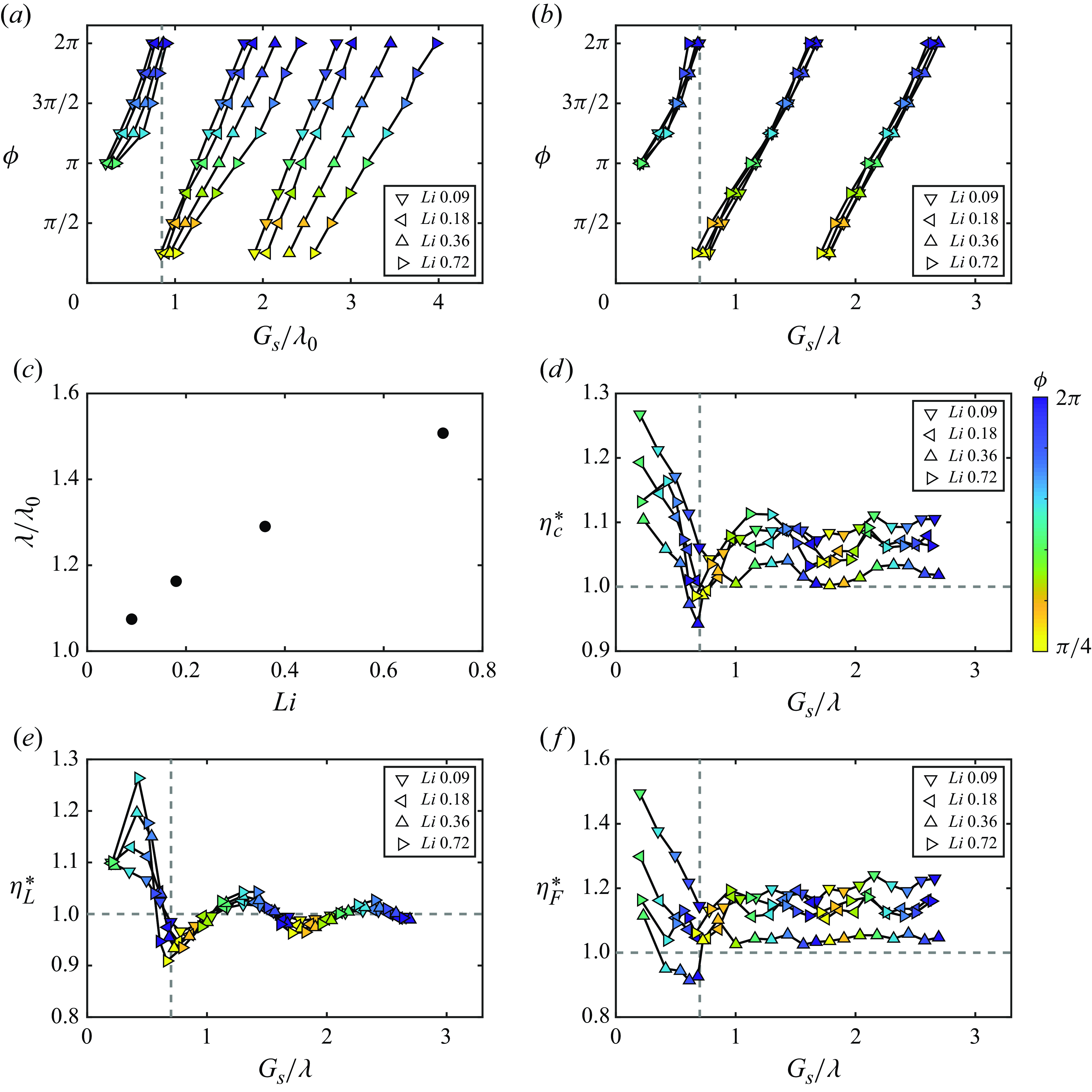
Figure 8. In-line stable gap distances scale with the actual wake wavelength, $\lambda$
, rather than the nominal wavelength,
$\lambda$
, rather than the nominal wavelength, $\lambda _{0}$
, for varying
$\lambda _{0}$
, for varying $Li$
. The pitching amplitude is
$Li$
. The pitching amplitude is $\theta _0 = 7.5^{\circ }$
. The grey vertical dashed lines represent
$\theta _0 = 7.5^{\circ }$
. The grey vertical dashed lines represent $G_{s}/\lambda _{0}=0.85$
and
$G_{s}/\lambda _{0}=0.85$
and $G_{s}/\lambda =0.7$
where the wavelengths are calculated/measured for the isolated leader. Stable gap distances scaled by
$G_{s}/\lambda =0.7$
where the wavelengths are calculated/measured for the isolated leader. Stable gap distances scaled by $(a)$
$(a)$ $\lambda _{0}$
and
$\lambda _{0}$
and $(b)$
$(b)$ $\lambda$
.
$\lambda$
. $(c)$
Wake wavelength compared with the nominal wavelength as a function of the Lighthill number. The mean value of
$(c)$
Wake wavelength compared with the nominal wavelength as a function of the Lighthill number. The mean value of $\lambda _{0}$
at each Lighthill nubmber in
$\lambda _{0}$
at each Lighthill nubmber in $(a)$
is used here, which is nearly equal to
$(a)$
is used here, which is nearly equal to $\lambda _{0}$
of the isolated counterparts (less than 5 % difference).
$\lambda _{0}$
of the isolated counterparts (less than 5 % difference). $(d)$
Normalised collective efficiency as a function of the normalised gap distance.
$(d)$
Normalised collective efficiency as a function of the normalised gap distance. $(e)$
Normalised leader efficiency as a function of the normalised gap distance.
$(e)$
Normalised leader efficiency as a function of the normalised gap distance. $(f)$
Normalised follower efficiency as a function of the normalised gap distance.
$(f)$
Normalised follower efficiency as a function of the normalised gap distance.
Figure 8(d) presents the normalised collective efficiency as a function of the normalised stable gap distances. There is an efficiency benefit for schooling ( $\eta _{c}^* \gt 1$
) at nearly all stable positions and the maximum efficiency enhancement is achieved for compact arrangements with
$\eta _{c}^* \gt 1$
) at nearly all stable positions and the maximum efficiency enhancement is achieved for compact arrangements with $G_{s}/\lambda \lt 0.7$
for all
$G_{s}/\lambda \lt 0.7$
for all $Li$
. Regardless of the Lighthill number, the collective efficiency has successive peaks that have gap distances one wavelength apart and nearly all of the peaks in efficiency occur for
$Li$
. Regardless of the Lighthill number, the collective efficiency has successive peaks that have gap distances one wavelength apart and nearly all of the peaks in efficiency occur for $\phi \approx \pi$
while nearly all of the troughs occur for
$\phi \approx \pi$
while nearly all of the troughs occur for $\phi \approx 0$
. Moreover, the maximum efficiency enhancement decreases with increasing Lighthill number from
$\phi \approx 0$
. Moreover, the maximum efficiency enhancement decreases with increasing Lighthill number from $Li = 0.09$
to
$Li = 0.09$
to $0.36$
and then increases with further increases in
$0.36$
and then increases with further increases in $Li$
. Further simulations are presented in Appendix B that more finely resolve the performance variations as the Lighthill number is varied from
$Li$
. Further simulations are presented in Appendix B that more finely resolve the performance variations as the Lighthill number is varied from $0.36 \leqslant Li \leqslant 0.72$
. Even though the data represent the same impingement timing between the leader’s vortices and the follower’s motion due to the proportional change in spacing and phase synchrony, in non-compact formations the collective efficiency enhancement differs. This indicates that more than a vortex–body mechanism is at play. In fact, there are both efficiency enhancements on the leader (figure 8
e) from body–body interactions and on the follower (figure 8
f) from vortex–body interactions. The leader’s efficiency presented in figure 8(e) shows that a phase synchrony of
$0.36 \leqslant Li \leqslant 0.72$
. Even though the data represent the same impingement timing between the leader’s vortices and the follower’s motion due to the proportional change in spacing and phase synchrony, in non-compact formations the collective efficiency enhancement differs. This indicates that more than a vortex–body mechanism is at play. In fact, there are both efficiency enhancements on the leader (figure 8
e) from body–body interactions and on the follower (figure 8
f) from vortex–body interactions. The leader’s efficiency presented in figure 8(e) shows that a phase synchrony of $\phi \approx 5\pi /4$
will maximise efficiency while
$\phi \approx 5\pi /4$
will maximise efficiency while $\phi \approx \pi /4$
will minimise it regardless of the gap spacing. This is an indication of a direct body–body interaction since the effect is upstream and only depends upon the phase synchrony between the foils. In the body–body interaction, the bound vortex of the follower alters the incoming flow encountered by the leader and affects the leader’s performance. The dependence of the bound vortex of the follower on the phase synchrony leads to the dependence of the leader’s performance on the phase synchrony. In contrast, the follower’s efficiency presented in figure 8(f) shows that when the gap spacing and phase synchrony change proportionally then there is no preferred phase to maximise the efficiency, at least in non-compact formations with
$\phi \approx \pi /4$
will minimise it regardless of the gap spacing. This is an indication of a direct body–body interaction since the effect is upstream and only depends upon the phase synchrony between the foils. In the body–body interaction, the bound vortex of the follower alters the incoming flow encountered by the leader and affects the leader’s performance. The dependence of the bound vortex of the follower on the phase synchrony leads to the dependence of the leader’s performance on the phase synchrony. In contrast, the follower’s efficiency presented in figure 8(f) shows that when the gap spacing and phase synchrony change proportionally then there is no preferred phase to maximise the efficiency, at least in non-compact formations with $G_{s}/\lambda \gt 0.7$
. This is indicative of a vortex–body interaction. In the vortex–body interaction, the wake vortices of the leader alter the incoming flow encountered by the follower and affect the follower’s performance. However, unlike the bound vortex, wake vortices depend on both the gap spacing and phase synchrony, leading to the disappearance of the optimum phase for maximising the follower’s performance.
$G_{s}/\lambda \gt 0.7$
. This is indicative of a vortex–body interaction. In the vortex–body interaction, the wake vortices of the leader alter the incoming flow encountered by the follower and affect the follower’s performance. However, unlike the bound vortex, wake vortices depend on both the gap spacing and phase synchrony, leading to the disappearance of the optimum phase for maximising the follower’s performance.
3.3. Varying the pitching amplitude
For the free-swimming simulations presented in this section, the Lighthill number is fixed at $Li =0.36$
while the pitching amplitude and phase synchrony vary over the ranges of
$Li =0.36$
while the pitching amplitude and phase synchrony vary over the ranges of $7.5^{\circ } \leqslant \theta _0 \leqslant 30^{\circ }$
and
$7.5^{\circ } \leqslant \theta _0 \leqslant 30^{\circ }$
and $0 \leqslant \phi \leqslant 2\pi$
, respectively (see varying
$0 \leqslant \phi \leqslant 2\pi$
, respectively (see varying $\theta _0$
in table 1). Figure 9(a) presents the stable gap distances normalised by the nominal wake wavelength as a function of the phase difference. Like the cases of varying the Lighthill number, the data points with the same pitching amplitude in figure 9(a) have nearly equal speeds and nominal wake wavelengths, which are within a
$\theta _0$
in table 1). Figure 9(a) presents the stable gap distances normalised by the nominal wake wavelength as a function of the phase difference. Like the cases of varying the Lighthill number, the data points with the same pitching amplitude in figure 9(a) have nearly equal speeds and nominal wake wavelengths, which are within a $5\,\%$
variation compared with those of their isolated counterparts. Unlike the stable gap distances with varying
$5\,\%$
variation compared with those of their isolated counterparts. Unlike the stable gap distances with varying $Li$
, the nominal wake wavelength can provide a good collapse with varying amplitude. In figure 9(b), the stable gap distances normalised by the actual wake wavelength are presented including the data for both varying Lighthill number and varying amplitude. It is found that the actual wake wavelength can provide an improved collapse of the data over the nominal wavelength especially when considering variations in both the pitching amplitude and Lighthill number. Also, a linear relationship between the phase difference and the normalised stable gap distances,
$Li$
, the nominal wake wavelength can provide a good collapse with varying amplitude. In figure 9(b), the stable gap distances normalised by the actual wake wavelength are presented including the data for both varying Lighthill number and varying amplitude. It is found that the actual wake wavelength can provide an improved collapse of the data over the nominal wavelength especially when considering variations in both the pitching amplitude and Lighthill number. Also, a linear relationship between the phase difference and the normalised stable gap distances,
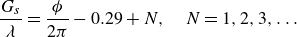 \begin{align} \frac {G_{s}}{\lambda } = \frac {\phi }{2\pi } -0.29 + N, \quad N = 1,2,3,\ldots \end{align}
is observed, which is represented by the black dashed lines and determined by linear regression with the data. Figure 9(c) shows that $\lambda /\lambda _{0}$
maintains a nearly constant ratio with variations in amplitude, which is why there is a good collapse of the stable gap distances across a range of amplitudes regardless of whether
$\lambda /\lambda _{0}$
maintains a nearly constant ratio with variations in amplitude, which is why there is a good collapse of the stable gap distances across a range of amplitudes regardless of whether $\lambda$
or
$\lambda$
or $\lambda _0$
is used as a scaling factor. Figure 9(d) presents the normalised collective efficiency as a function of the normalised stable gap distance. The maximum efficiency enhancement is achieved for
$\lambda _0$
is used as a scaling factor. Figure 9(d) presents the normalised collective efficiency as a function of the normalised stable gap distance. The maximum efficiency enhancement is achieved for $G_s/\lambda \lt 0.7$
for all pitching amplitudes just as in the varying Lighthill number data. As observed previously, peaks in efficiency enhancement occur at
$G_s/\lambda \lt 0.7$
for all pitching amplitudes just as in the varying Lighthill number data. As observed previously, peaks in efficiency enhancement occur at $\phi \approx \pi$
and troughs occur at
$\phi \approx \pi$
and troughs occur at $\phi \approx 0$
, except for
$\phi \approx 0$
, except for $\theta _{0} = 30^{\circ }$
where those trends are flipped. Benefits in propulsive efficiency of in-line schooling (
$\theta _{0} = 30^{\circ }$
where those trends are flipped. Benefits in propulsive efficiency of in-line schooling ( $\eta _{c}^*\gt 1$
) are observed at nearly all stable gap distances over the range of
$\eta _{c}^*\gt 1$
) are observed at nearly all stable gap distances over the range of $7.5^{\circ } \leqslant \theta _{0} \leqslant 22.5^{\circ }$
with
$7.5^{\circ } \leqslant \theta _{0} \leqslant 22.5^{\circ }$
with $\theta _{0} = 15^{\circ }$
giving the global peak efficiency benefit when
$\theta _{0} = 15^{\circ }$
giving the global peak efficiency benefit when $G_s/\lambda \lt 0.7$
and
$G_s/\lambda \lt 0.7$
and $\theta _{0} = 22.5^{\circ }$
giving the local peak efficiency benefits when
$\theta _{0} = 22.5^{\circ }$
giving the local peak efficiency benefits when $G_s/\lambda \gt 0.7$
. In contrast, there is an efficiency penalty at the pitching amplitude of
$G_s/\lambda \gt 0.7$
. In contrast, there is an efficiency penalty at the pitching amplitude of $30^{\circ }$
. Further simulations are presented in Appendix B that more finely resolve the performance variations as the amplitude is varied from
$30^{\circ }$
. Further simulations are presented in Appendix B that more finely resolve the performance variations as the amplitude is varied from $22.5^{\circ } \leqslant \theta _0 \leqslant 30^\circ$
.
$22.5^{\circ } \leqslant \theta _0 \leqslant 30^\circ$
.
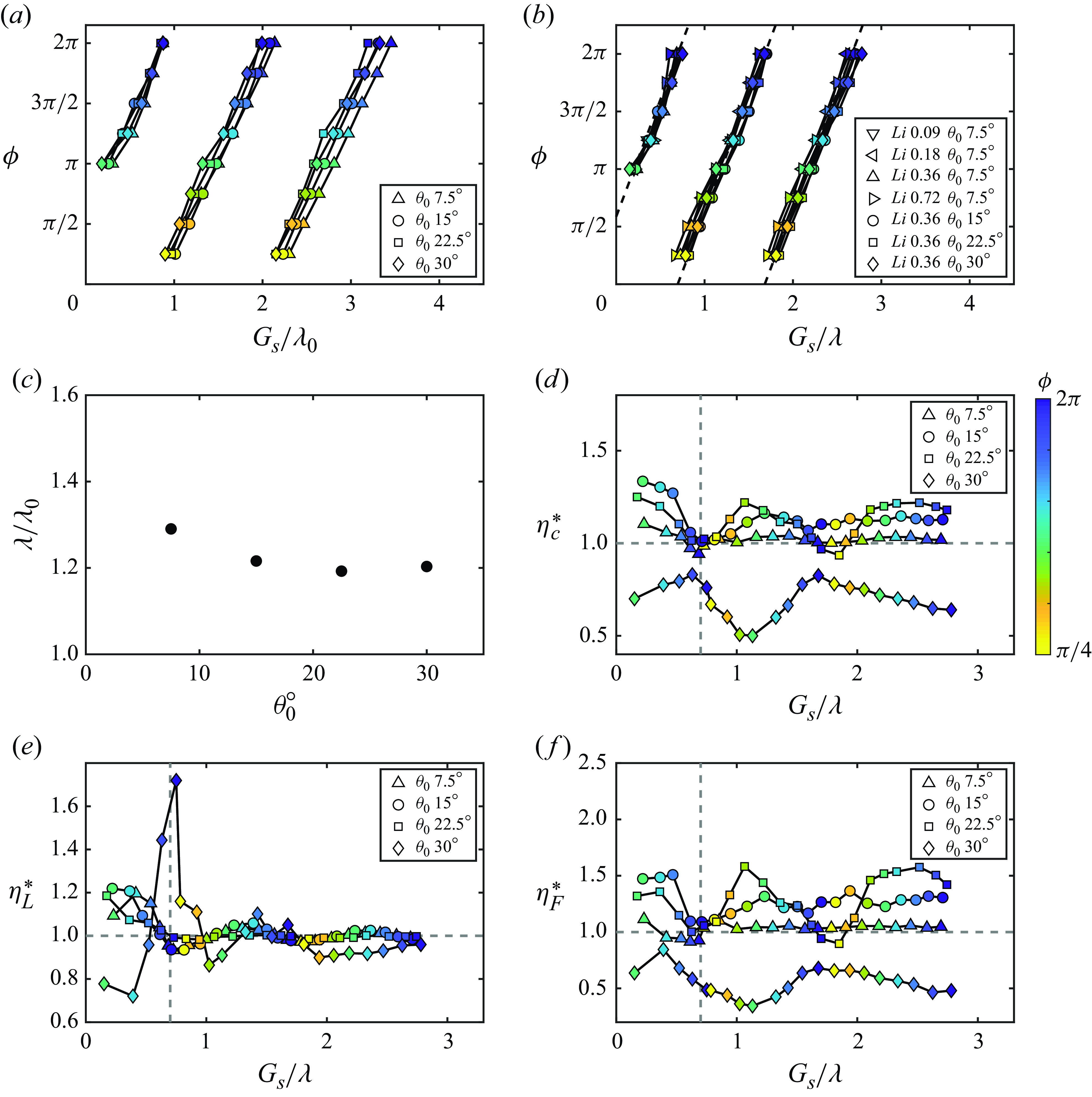
Figure 9. The stable gap distances scale with the leader’s wake wavelength regardless of variations in $Li$
or
$Li$
or $\theta _{0}$
. The Lighthill number is
$\theta _{0}$
. The Lighthill number is $Li = 0.36$
for
$Li = 0.36$
for $(a)$
,
$(a)$
, $(c)$
and
$(c)$
and $(d)$
. The wavelengths are calculated/measured for the isolated leader. Stable gap distances scaled by
$(d)$
. The wavelengths are calculated/measured for the isolated leader. Stable gap distances scaled by $(a)$
$(a)$ $\lambda _{0}$
and
$\lambda _{0}$
and $(b)$
$(b)$ $\lambda$
(with the data of varying
$\lambda$
(with the data of varying $Li$
included). Black dashed lines represent the linear relationship
$Li$
included). Black dashed lines represent the linear relationship $G_s/\lambda = \phi /(2\pi ) -0.29 + N, \, N = 1,2,3,\ldots$
.
$G_s/\lambda = \phi /(2\pi ) -0.29 + N, \, N = 1,2,3,\ldots$
. $(c)$
Wake wavelength compared with the nominal wavelength as a function of the pitching amplitude. The mean value of
$(c)$
Wake wavelength compared with the nominal wavelength as a function of the pitching amplitude. The mean value of $\lambda _{0}$
at each pitching amplitude in
$\lambda _{0}$
at each pitching amplitude in $(a)$
is used here, which is nearly equal to
$(a)$
is used here, which is nearly equal to $\lambda _{0}$
of the isolated counterparts (less than 5 % difference).
$\lambda _{0}$
of the isolated counterparts (less than 5 % difference). $(d)$
Normalised collective efficiency as a function of the normalised gap distance. The grey vertical dashed line represents
$(d)$
Normalised collective efficiency as a function of the normalised gap distance. The grey vertical dashed line represents $G_s/\lambda =0.7$
.
$G_s/\lambda =0.7$
. $(e)$
Normalised leader efficiency as a function of the normalised gap distance.
$(e)$
Normalised leader efficiency as a function of the normalised gap distance. $(f)$
Normalised follower efficiency as a function of the normalised gap distance.
$(f)$
Normalised follower efficiency as a function of the normalised gap distance.
Figures 9(e) and 9(f) present the normalised efficiencies of the leader and the follower, respectively. In figure 9(e), like the case of varying the Lighthill number, the leader’s efficiency is maximised at $\phi \approx 5\pi /4$
and is minimised at
$\phi \approx 5\pi /4$
and is minimised at $\phi \approx \pi /4$
regardless of gap spacing, except for
$\phi \approx \pi /4$
regardless of gap spacing, except for $\theta _{0} = 30^{\circ }$
. At the amplitude of
$\theta _{0} = 30^{\circ }$
. At the amplitude of $\theta _{0} = 30^{\circ }$
, the phase synchrony that maximises efficiency shifts to
$\theta _{0} = 30^{\circ }$
, the phase synchrony that maximises efficiency shifts to $\phi \approx 2\pi$
, and the phase that minimises efficiency shifts to
$\phi \approx 2\pi$
, and the phase that minimises efficiency shifts to $\phi \approx \pi$
. Like the case of varying the Lighthill number, the leader’s performance is driven by a direct body–body interaction. However, the amplitude of
$\phi \approx \pi$
. Like the case of varying the Lighthill number, the leader’s performance is driven by a direct body–body interaction. However, the amplitude of $\theta _{0} = 30^{\circ }$
generates stronger leading-edge vortex, which alters the foils’ bound circulations and results in a different body–body interaction. Figure 9(f) presents that, like the case of varying the Lighthill number, the follower’s performance is driven by a vortex–body interaction and has no preferred phase to maximise efficiency in non-compact formations with
$\theta _{0} = 30^{\circ }$
generates stronger leading-edge vortex, which alters the foils’ bound circulations and results in a different body–body interaction. Figure 9(f) presents that, like the case of varying the Lighthill number, the follower’s performance is driven by a vortex–body interaction and has no preferred phase to maximise efficiency in non-compact formations with $G_{s}/\lambda \lt 0.7$
, except for the amplitudes of
$G_{s}/\lambda \lt 0.7$
, except for the amplitudes of $\theta _{0} = 22.5^{\circ }$
and
$\theta _{0} = 22.5^{\circ }$
and $30^{\circ }$
. At the large amplitudes, the bound circulation of the leader becomes stronger, leading to a larger variation of its downstream effect on the follower with the phase. Therefore, the performance of the follower has a larger variation with the phase at the amplitudes of
$30^{\circ }$
. At the large amplitudes, the bound circulation of the leader becomes stronger, leading to a larger variation of its downstream effect on the follower with the phase. Therefore, the performance of the follower has a larger variation with the phase at the amplitudes of $\theta _{0} = 22.5^{\circ }$
and
$\theta _{0} = 22.5^{\circ }$
and $30^{\circ }$
. Furthermore, it is discovered that the penalty of the collective efficiency at
$30^{\circ }$
. Furthermore, it is discovered that the penalty of the collective efficiency at $\theta _{0} = 30^{\circ }$
is driven by the efficiency penalty of the follower.
$\theta _{0} = 30^{\circ }$
is driven by the efficiency penalty of the follower.
3.4. Revealing the vortex dynamics behind performance variation
In order to illustrate the performance variation with varying Lighthill number and amplitude, in this section, we focus on the data points of $\phi = \pi$
at
$\phi = \pi$
at $G_{s}/\lambda \approx 1.2$
in figures 8(d) and 9(d). These points show similar normalised leader efficiency close to
$G_{s}/\lambda \approx 1.2$
in figures 8(d) and 9(d). These points show similar normalised leader efficiency close to $1$
in figures 8(e) and 9(e). The variation of the collective efficiency enhancement is driven by the variation of the normalised follower efficiency in figures 8(f) and 9(f). Therefore, we only need to focus on the variation of the normalised follower efficiency to explain the variation of the normalised collective efficiency for both varying Lighthill number and amplitude cases. Since the leader has an efficiency close to the isolated swimmer, we are interested in the efficiency difference between the follower and the leader. Moreover, the two foils have equal free stream velocities and thrusts, which means that the foil’s efficiency difference is directly generated by their difference in power.
$1$
in figures 8(e) and 9(e). The variation of the collective efficiency enhancement is driven by the variation of the normalised follower efficiency in figures 8(f) and 9(f). Therefore, we only need to focus on the variation of the normalised follower efficiency to explain the variation of the normalised collective efficiency for both varying Lighthill number and amplitude cases. Since the leader has an efficiency close to the isolated swimmer, we are interested in the efficiency difference between the follower and the leader. Moreover, the two foils have equal free stream velocities and thrusts, which means that the foil’s efficiency difference is directly generated by their difference in power.
Figure 10. Vorticity field and normalised power saving, $\Delta P^{*} = (P_{L} - P_{F})/P_{L,\textit{total}}$
, along the follower’s chord for
$\Delta P^{*} = (P_{L} - P_{F})/P_{L,\textit{total}}$
, along the follower’s chord for $(a)$
and
$(a)$
and $(b)$
$(b)$ $Li = 0.09$
and
$Li = 0.09$
and $\theta _{0} = 7.5^{\circ }$
;
$\theta _{0} = 7.5^{\circ }$
; $(c)$
and
$(c)$
and $(d)$
$(d)$ $Li = 0.36$
and
$Li = 0.36$
and $\theta _{0} = 7.5^{\circ }$
;
$\theta _{0} = 7.5^{\circ }$
; $(e)$
and
$(e)$
and $(f)$
$(f)$ $Li = 0.72$
and
$Li = 0.72$
and $\theta _{0} = 7.5^{\circ }$
. The time instant is
$\theta _{0} = 7.5^{\circ }$
. The time instant is $t/T = 0.46$
for
$t/T = 0.46$
for $(a)$
to
$(a)$
to $(b)$
, and is
$(b)$
, and is $t/T = 0.92$
for
$t/T = 0.92$
for $(e)$
and
$(e)$
and $(f)$
. The swimmers have a phase difference of
$(f)$
. The swimmers have a phase difference of $\phi = \pi$
and a normalised stable gap distance of
$\phi = \pi$
and a normalised stable gap distance of $G_{s}/\lambda \approx 1.21$
.
$G_{s}/\lambda \approx 1.21$
.
Figure 10 presents the vorticity field and the relative power savings at the time instant when the largest power difference occurs for varying the Lighthill number from $Li = 0.09$
to
$Li = 0.09$
to $0.72$
with the amplitude fixed at
$0.72$
with the amplitude fixed at $\theta _{0} = 7.5^{\circ }$
. A positive relative power saving indicates that the follower consumes less power than the leader, and vice versa. According to figure 8(f), the relative power savings decreases with increasing
$\theta _{0} = 7.5^{\circ }$
. A positive relative power saving indicates that the follower consumes less power than the leader, and vice versa. According to figure 8(f), the relative power savings decreases with increasing $Li$
from
$Li$
from $Li = 0.09$
to
$Li = 0.09$
to $0.36$
, and then increases with further increases in
$0.36$
, and then increases with further increases in $Li$
. In figure 10(a), when the Lighthill number is
$Li$
. In figure 10(a), when the Lighthill number is $Li = 0.09$
, the leader is pitching downwards while the follower is pitching upwards. A negative leading-edge vortex is present near the follower’s leading edge above the follower’s upper surface. A positive trailing-edge vortex of the leader is about to impinge on the follower. In addition, below the follower’s lower surface, there is a vortex pair near its trailing edge. In figure 10(b), there are three regions along the chord that increase or decrease the follower’s power savings from its leading edge to trailing edge. In region 1, which is near the follower’s leading edge, the leader’s positive trailing-edge vortex and the follower’s negative leading-edge vortex pair together and form a jet pointing upwards. This jet increases the follower’s angle of attack and moves the stagnation point created by the incoming flow to the follower’s lower surface, which increases the pressure and force acting in the same direction as the foil’s motion. Therefore, the follower’s power is reduced, leading to positive power savings. In region 2, the velocity on the lower surface of the follower is increased by the velocity induced from the negative vortex of the vortex pair, which, thus, decreases the pressure on the lower surface. This increases the force opposing the foil’s motion, generating negative power savings. In contrast, the positive vortex of the vortex pair decreases the velocity on the lower surface in region 3, which increases the force acting in the same direction as the foil’s motion and results in positive power savings. Furthermore, the force in region 3 is the farthest from the follower’s pitch axis and has the largest moment arm. Therefore, region 3 generates the largest power difference. When the Lighthill number is increased to
$Li = 0.09$
, the leader is pitching downwards while the follower is pitching upwards. A negative leading-edge vortex is present near the follower’s leading edge above the follower’s upper surface. A positive trailing-edge vortex of the leader is about to impinge on the follower. In addition, below the follower’s lower surface, there is a vortex pair near its trailing edge. In figure 10(b), there are three regions along the chord that increase or decrease the follower’s power savings from its leading edge to trailing edge. In region 1, which is near the follower’s leading edge, the leader’s positive trailing-edge vortex and the follower’s negative leading-edge vortex pair together and form a jet pointing upwards. This jet increases the follower’s angle of attack and moves the stagnation point created by the incoming flow to the follower’s lower surface, which increases the pressure and force acting in the same direction as the foil’s motion. Therefore, the follower’s power is reduced, leading to positive power savings. In region 2, the velocity on the lower surface of the follower is increased by the velocity induced from the negative vortex of the vortex pair, which, thus, decreases the pressure on the lower surface. This increases the force opposing the foil’s motion, generating negative power savings. In contrast, the positive vortex of the vortex pair decreases the velocity on the lower surface in region 3, which increases the force acting in the same direction as the foil’s motion and results in positive power savings. Furthermore, the force in region 3 is the farthest from the follower’s pitch axis and has the largest moment arm. Therefore, region 3 generates the largest power difference. When the Lighthill number is increased to $0.36$
in figure 10(c), the vortex pair moves closer to the follower’s leading edge due to the reduced wake wavelength, so the effect of the negative vortex below the lower surface moves towards the leading edge, which results in a narrower region 1 in figure 10(d). In addition, the moment arm of the force in region 3 becomes smaller, leading to smaller power savings. Consequently, the total power savings of the follower is reduced. When the Lighthill number is further increased to
$0.36$
in figure 10(c), the vortex pair moves closer to the follower’s leading edge due to the reduced wake wavelength, so the effect of the negative vortex below the lower surface moves towards the leading edge, which results in a narrower region 1 in figure 10(d). In addition, the moment arm of the force in region 3 becomes smaller, leading to smaller power savings. Consequently, the total power savings of the follower is reduced. When the Lighthill number is further increased to $Li = 0.72$
in figure 10(e), the leader shows a slightly downwards deflected wake because of an increased Strouhal number. This asymmetry alters the impingement of the leader’s trailing-edge vortices on the follower, which leads to a different time instant when the largest power difference occurs. In figure 10(e), the leader is pitching upwards while the follower is pitching downwards, the opposite of the previous cases. The majority of the leader’s trailing-edge vortices move below the lower surface of the follower. Because of the wake asymmetry, the follower’s leading edge is vertically in the middle of the leader’s positive trailing-edge vortex when the positive vortex impinges on the follower, which creates even leading-edge suction on the upper and lower surfaces of the follower and suppresses the generation of the follower’s leading-edge vortex. Therefore, region 3 disappears in figure 10(f). In region 1, the leader’s negative and positive trailing-edge vortices form a jet pointing downwards. This jet increases the follower’s angle of attack and moves the stagnation point created by the incoming flow to the follower’s upper surface, which increases the force acting in the same direction as the foil’s motion. Like the previous cases, the negative trailing-edge vortex of the leader decreases the pressure on the follower’s lower surface. However, the follower is pitching downwards in this case, which flips the effect of the negative vortex and leads to positive power savings. Therefore, the total power savings of the follower becomes larger.
$Li = 0.72$
in figure 10(e), the leader shows a slightly downwards deflected wake because of an increased Strouhal number. This asymmetry alters the impingement of the leader’s trailing-edge vortices on the follower, which leads to a different time instant when the largest power difference occurs. In figure 10(e), the leader is pitching upwards while the follower is pitching downwards, the opposite of the previous cases. The majority of the leader’s trailing-edge vortices move below the lower surface of the follower. Because of the wake asymmetry, the follower’s leading edge is vertically in the middle of the leader’s positive trailing-edge vortex when the positive vortex impinges on the follower, which creates even leading-edge suction on the upper and lower surfaces of the follower and suppresses the generation of the follower’s leading-edge vortex. Therefore, region 3 disappears in figure 10(f). In region 1, the leader’s negative and positive trailing-edge vortices form a jet pointing downwards. This jet increases the follower’s angle of attack and moves the stagnation point created by the incoming flow to the follower’s upper surface, which increases the force acting in the same direction as the foil’s motion. Like the previous cases, the negative trailing-edge vortex of the leader decreases the pressure on the follower’s lower surface. However, the follower is pitching downwards in this case, which flips the effect of the negative vortex and leads to positive power savings. Therefore, the total power savings of the follower becomes larger.
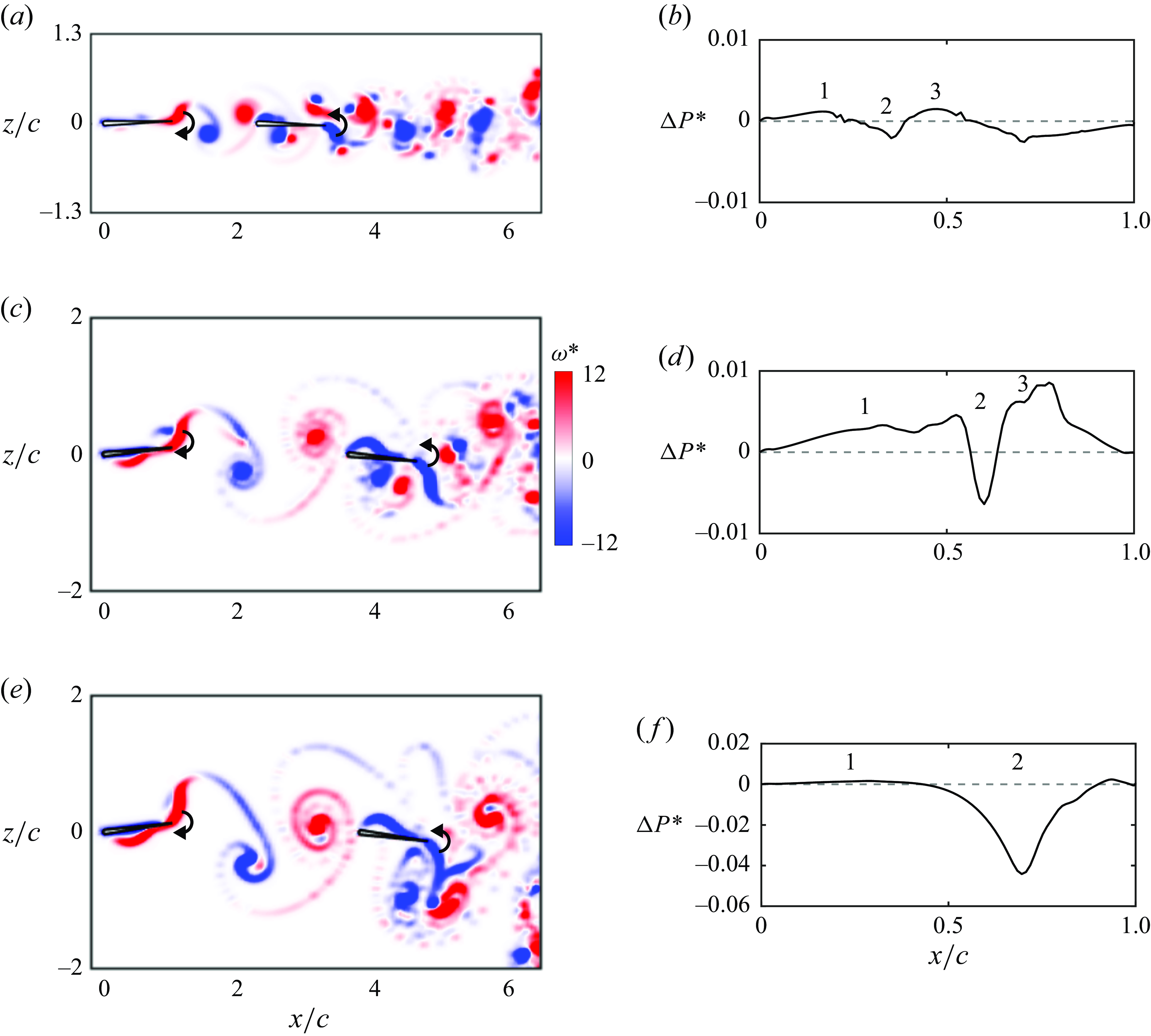
Figure 11. Vorticity field and normalised power saving, $\Delta P^{*} = (P_{L} - P_{F})/P_{L,\textit{total}}$
, along the follower’s chord for
$\Delta P^{*} = (P_{L} - P_{F})/P_{L,\textit{total}}$
, along the follower’s chord for $(a)$
and
$(a)$
and $(b)$
$(b)$ $Li = 0.36$
and
$Li = 0.36$
and $\theta _{0} = 7.5^{\circ }$
;
$\theta _{0} = 7.5^{\circ }$
; $(c)$
and
$(c)$
and $(d)$
$(d)$ $Li = 0.36$
and
$Li = 0.36$
and $\theta _{0} = 22.5^{\circ }$
;
$\theta _{0} = 22.5^{\circ }$
; $(e)$
and
$(e)$
and $(f)$
$(f)$ $Li = 0.36$
and
$Li = 0.36$
and $\theta _{0} = 30^{\circ }$
. The time instant is
$\theta _{0} = 30^{\circ }$
. The time instant is $t/T = 0.46$
. The swimmers have a phase difference of
$t/T = 0.46$
. The swimmers have a phase difference of $\phi = \pi$
and a normalised stable gap distance of
$\phi = \pi$
and a normalised stable gap distance of $G_{s}/\lambda \approx 1.21$
.
$G_{s}/\lambda \approx 1.21$
.
Figure 11 presents the vorticity field and the relative power savings at the time instant when the largest power difference occurs for varying amplitude from $\theta _{0} = 7.5^{\circ }$
to
$\theta _{0} = 7.5^{\circ }$
to $30^{\circ }$
with the Lighthill number fixed at
$30^{\circ }$
with the Lighthill number fixed at $Li=0.36$
. According to figure 9(f), the power savings of the follower increases as the amplitude increases from
$Li=0.36$
. According to figure 9(f), the power savings of the follower increases as the amplitude increases from $7.5^{\circ }$
to
$7.5^{\circ }$
to $22.5^{\circ }$
, and then transforms into a power penalty for further increases in amplitude. In figure 11, the leader is pitching downwards while the follower is pitching upwards. At the amplitude of
$22.5^{\circ }$
, and then transforms into a power penalty for further increases in amplitude. In figure 11, the leader is pitching downwards while the follower is pitching upwards. At the amplitude of $7.5^{\circ }$
, as demonstrated above, there are three regions that increase or decrease the power savings of the follower in figure 11(b) due to the leading-edge vortex above its upper surface and the vortex pair below its lower surface in figure 11(a). When the amplitude is increased to
$7.5^{\circ }$
, as demonstrated above, there are three regions that increase or decrease the power savings of the follower in figure 11(b) due to the leading-edge vortex above its upper surface and the vortex pair below its lower surface in figure 11(a). When the amplitude is increased to $\theta _{0} = 22.5^{\circ }$
in figure 11(c), the vortex pair moves closer to the trailing edge of the follower, due to the increased wake wavelength, which moves the effect of the negative vortex of the vortex pair farther downstream. Therefore, region 1 becomes wider in figure 11(d). In addition, the moment arm of the force in region 3 is increased, which increases the magnitude of the power savings in region 3. In region 2 on the follower’s upper surface, unlike the case of
$\theta _{0} = 22.5^{\circ }$
in figure 11(c), the vortex pair moves closer to the trailing edge of the follower, due to the increased wake wavelength, which moves the effect of the negative vortex of the vortex pair farther downstream. Therefore, region 1 becomes wider in figure 11(d). In addition, the moment arm of the force in region 3 is increased, which increases the magnitude of the power savings in region 3. In region 2 on the follower’s upper surface, unlike the case of $\theta _{0} = 7.5 ^{\circ }$
, the follower’s negative leading-edge vortex sheet reattaches to its upper surface. The velocity induced from the negative vortex sheet decreases the velocity on the upper surface, which increases the surface pressure and, therefore, increases the force acting to oppose the foil’s motion. Therefore, the power penalty in region 2 becomes larger. However, regions 1 and 3 dominate the total power savings, so the total power savings of the follower is increased. As the amplitude is further increased to
$\theta _{0} = 7.5 ^{\circ }$
, the follower’s negative leading-edge vortex sheet reattaches to its upper surface. The velocity induced from the negative vortex sheet decreases the velocity on the upper surface, which increases the surface pressure and, therefore, increases the force acting to oppose the foil’s motion. Therefore, the power penalty in region 2 becomes larger. However, regions 1 and 3 dominate the total power savings, so the total power savings of the follower is increased. As the amplitude is further increased to $\theta _{0} = 30^{\circ }$
in figure 11(e), the follower’s leading-edge vortex sheet is detached from the follower near its leading edge and the power savings in region 1 becomes nearly negligible compared with the power penalty of region 2 in figure 11(f). Region 2 dominates the power penalty incurred at the amplitude of
$\theta _{0} = 30^{\circ }$
in figure 11(e), the follower’s leading-edge vortex sheet is detached from the follower near its leading edge and the power savings in region 1 becomes nearly negligible compared with the power penalty of region 2 in figure 11(f). Region 2 dominates the power penalty incurred at the amplitude of $\theta _{0} = 30^{\circ }$
, and its peak is increased because of the increased moment arm of the force generated by the leading-edge vortex sheet reattachment. Furthermore, the positive vortex of the vortex pair below the follower resides far from the follower and downstream of its trailing edge due to the increased wake wavelength, which leads to the disappearance of region 3.
$\theta _{0} = 30^{\circ }$
, and its peak is increased because of the increased moment arm of the force generated by the leading-edge vortex sheet reattachment. Furthermore, the positive vortex of the vortex pair below the follower resides far from the follower and downstream of its trailing edge due to the increased wake wavelength, which leads to the disappearance of region 3.
From this detailed examination of the vortex dynamics and power savings it is observed that the positive power savings of the follower is generated in regions 1 and 3, which is driven by the location of the vortex pair. When the vortex pair resides closer to the follower’s leading edge, region 1 becomes narrower, and the magnitude of the power savings in region 3 is reduced, leading to smaller total power savings. When the vortex pair resides farther downstream, region 1 becomes wider, and the magnitude of the power savings in region 3 is increased, leading to larger total power savings. However, when the red vortex of the vortex pair resides downstream of the follower’s trailing edge, region 3 disappears, thereby lowering the total power savings to even reflect a power penalty. Therefore, if the vortex pair is close to the foil and reaches the trailing edge after a half-cycle of foil motion it will then maximise the power savings of the follower and, consequently, the collective efficiency. This leads to the conclusion that the key driver that maximises the efficiency of the follower is that the wake wavelength generated by the leader and non-dimensionalised by the chord of the follower should be approximately two. That is,
 \begin{align} \lambda /c \approx 2 \quad \text{maximises the follower efficiency.} \end{align}
Figure 12. Maximum normalised follower efficiency as a function of $\lambda /c$
.
$\lambda /c$
.
Figure 12 presents the maximum normalised follower efficiency as a function of $\lambda /c$
for the cases in § § 3.2 and 3.3 and Appendix B. To better resolve the optimal condition, we identified three additional data points at
$\lambda /c$
for the cases in § § 3.2 and 3.3 and Appendix B. To better resolve the optimal condition, we identified three additional data points at $\lambda /c\approx 2$
(coloured markers). As predicted by the insights from the above vortex analysis, it is discovered that the global maximum of the follower’s efficiency enhancement occurs at
$\lambda /c\approx 2$
(coloured markers). As predicted by the insights from the above vortex analysis, it is discovered that the global maximum of the follower’s efficiency enhancement occurs at $\lambda /c \approx 2$
.
$\lambda /c \approx 2$
.
3.5. Scaling the wake wavelength
As shown in the previous sections, stable gap distances of in-line schooling scale with the wake wavelength, $\lambda$
, of the isolated leader rather than the nominal wake wavelength,
$\lambda$
, of the isolated leader rather than the nominal wake wavelength, $\lambda _{0}$
. In addition, the ratio of the wake wavelength over the follower’s chord length determines the global maximum of the follower’s efficiency enhancement. Here, we present scaling laws to predict the wake wavelength from the Strouhal number and reduced frequency of the leader. In fact, the nominal wake wavelength is already a function of the reduced frequency,
$\lambda _{0}$
. In addition, the ratio of the wake wavelength over the follower’s chord length determines the global maximum of the follower’s efficiency enhancement. Here, we present scaling laws to predict the wake wavelength from the Strouhal number and reduced frequency of the leader. In fact, the nominal wake wavelength is already a function of the reduced frequency,
 \begin{gather} \lambda _{0} = \frac {c}{k}. \end{gather}
Therefore, we only need to provide a scaling law for the ratio of the wavelength over the nominal wavelength, which is equivalent to the speed of wake vortices relative to the nominal free stream speed,
 \begin{gather} \frac {\lambda }{\lambda _{0}} = \frac {U_{a}/f}{U/f} = \frac {U_{a}}{U}, \end{gather}
where $U_{a}$
is the velocity of a wake vortex advecting downstream. This is calculated as
$U_{a}$
is the velocity of a wake vortex advecting downstream. This is calculated as
 \begin{gather} U_{a} = U + U_{i}, \end{gather}
where $U_{i}$
is the induced streamwise velocity acting on a wake vortex from other wake vortices, which is approximated as the velocity induced by the two nearest vortices (figure 13
a). Therefore, the ratio of the wavelength over the nominal wavelength becomes
$U_{i}$
is the induced streamwise velocity acting on a wake vortex from other wake vortices, which is approximated as the velocity induced by the two nearest vortices (figure 13
a). Therefore, the ratio of the wavelength over the nominal wavelength becomes
 \begin{gather} \frac {\lambda }{\lambda _{0}} = 1 + U^*_{i}, \end{gather}
where $U^*_{i} = U_i/U$
. Based on the Biot–Savart law, the induced velocity is calculated as
$U^*_{i} = U_i/U$
. Based on the Biot–Savart law, the induced velocity is calculated as
 \begin{gather} U_{i} = \frac {\Gamma A}{\pi r^2} \quad \text{with} \quad r = \sqrt {\frac {U^2_{a}}{4f^2} + A^2}, \end{gather}
where $\Gamma$
is the strength of the wake vortices, and
$\Gamma$
is the strength of the wake vortices, and $r$
is the distance from the neighbouring vortices to the vortex of interest. Solving (3.7) gives (see Appendix A.1 for details)
$r$
is the distance from the neighbouring vortices to the vortex of interest. Solving (3.7) gives (see Appendix A.1 for details)
 \begin{gather} U^*_{i} = c_{1}\, k\,St, \end{gather}
where $c_1$
is a constant to be determined. We then have
$c_1$
is a constant to be determined. We then have
 \begin{gather} \frac {\lambda }{\lambda _{0}} = 1 + c_{1}\,k\, St. \end{gather}
The scaling law in (3.9) can be applied to both constrained and unconstrained pitching foils. However, the Strouhal number and reduced frequency of unconstrained foils are not known a priori since they depend on the mean swimming speed of the foils. We can provide an additional scaling law to predict these dimensionless variables as a function of the dimensionless input variables known a priori, namely, the dimensionless amplitude and Lighthill number. To do this, we begin with a scaling law for the thrust of pitching foils developed in Moored & Quinn (Reference Moored and Quinn2019),
 \begin{align} C_{T}^a & = c_{2}\phi _{1} + c_{3}\phi _{2} + c_{4}\phi _{3},\end{align}
 \begin{align} \phi _{1} & = 1,\end{align}
 \begin{align} \phi _{2} & = w(k) = \frac {3F}{2} - \frac {G}{2\pi k} + \frac {F}{\pi ^2 k^2} - (F^2 + G^2)\left (\frac {1}{\pi ^2k^2} + \frac {9}{4}\right ),\end{align}
 \begin{align} \phi _{3}& = A^*,\end{align}
where $C^a_{T} = \overline {T}/(\rho c s f^2 A^2)$
is the thrust normalised by the characteristic added mass force of a pitching foil,
$C^a_{T} = \overline {T}/(\rho c s f^2 A^2)$
is the thrust normalised by the characteristic added mass force of a pitching foil, $w(k)$
is the wake function,
$w(k)$
is the wake function, $F$
and
$F$
and $G$
are the real and imaginary components of Theodorsen’s lift deficiency function, respectively (Theodorsen Reference Theodorsen1935; Garrick Reference Garrick1936), and
$G$
are the real and imaginary components of Theodorsen’s lift deficiency function, respectively (Theodorsen Reference Theodorsen1935; Garrick Reference Garrick1936), and $c_{2}$
,
$c_{2}$
, $c_{3}$
and
$c_{3}$
and $c_{4}$
are constants to be determined. Under a high-frequency approximation, we have
$c_{4}$
are constants to be determined. Under a high-frequency approximation, we have
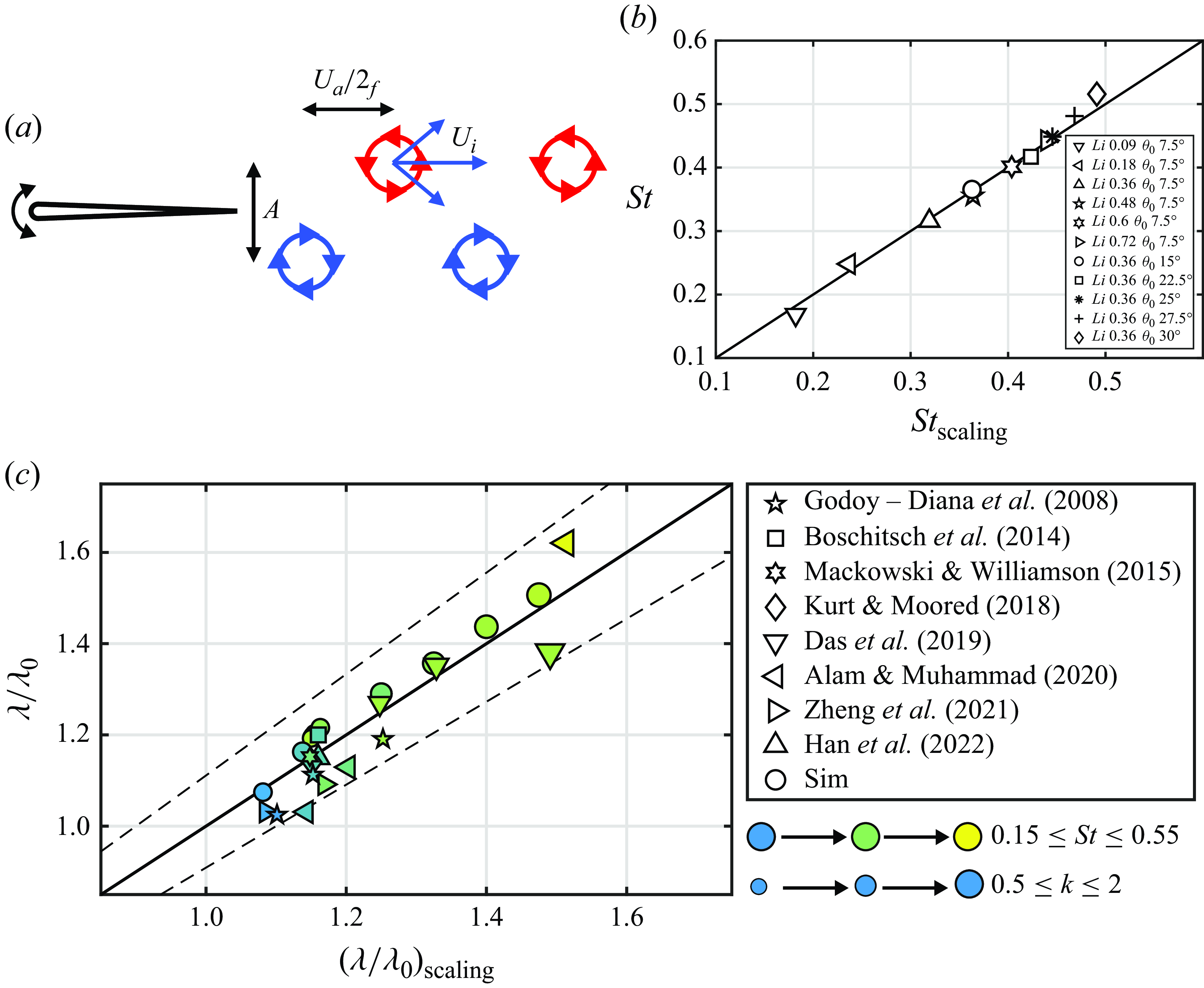
Figure 13. Proposed wavelength scaling law collapses data from two-dimensional experimental and numerical studies over a wide range of $St$
and
$St$
and $k$
.
$k$
. $(a)$
Schematic of a purely pitching foil and its wake vortices.
$(a)$
Schematic of a purely pitching foil and its wake vortices. $(b)$
The Strouhal number from unconstrained pitching foil simulations compared with the scaling relation. Here
$(b)$
The Strouhal number from unconstrained pitching foil simulations compared with the scaling relation. Here $St_{{scaling}}$
represents the Strouhal number predicted by the scaling relation in (3.17).
$St_{{scaling}}$
represents the Strouhal number predicted by the scaling relation in (3.17). $(c)$
Wavelength data compared with the scaling relation (3.9). Dashed lines represent
$(c)$
Wavelength data compared with the scaling relation (3.9). Dashed lines represent $\pm 10$
% error. These data cover unconstrained simulations from the current study as well as simulations and experiments from previous constrained studies for
$\pm 10$
% error. These data cover unconstrained simulations from the current study as well as simulations and experiments from previous constrained studies for $200 \leqslant Re \leqslant 59000$
(Godoy-diana et al. Reference Godoy-Diana, Aider and Wesfreid2008; Boschitsch et al. Reference Boschitsch, Dewey and Smits2014; Mackowski & Williamson Reference Mackowski and Williamson2015; Kurt & Moored Reference Kurt and Moored2018; Das et al. Reference Das, Shukla and Govardhan2019; Alam & Muhammad Reference Alam and Muhammad2020; Zheng et al. Reference Zheng, Pröbsting, Wang and Li2021; Han et al. Reference Han, Mivehchi, Kurt and Moored2022a
). The marker colour from blue to yellow represents increasing
$200 \leqslant Re \leqslant 59000$
(Godoy-diana et al. Reference Godoy-Diana, Aider and Wesfreid2008; Boschitsch et al. Reference Boschitsch, Dewey and Smits2014; Mackowski & Williamson Reference Mackowski and Williamson2015; Kurt & Moored Reference Kurt and Moored2018; Das et al. Reference Das, Shukla and Govardhan2019; Alam & Muhammad Reference Alam and Muhammad2020; Zheng et al. Reference Zheng, Pröbsting, Wang and Li2021; Han et al. Reference Han, Mivehchi, Kurt and Moored2022a
). The marker colour from blue to yellow represents increasing $St$
while the marker size from small to large represents increasing
$St$
while the marker size from small to large represents increasing $k$
. Note that for the current unconstrained simulations first
$k$
. Note that for the current unconstrained simulations first $St$
and
$St$
and $k$
are calculated with the scaling relations (3.17) and (3.18), which are then used in scaling relation (3.9) to find
$k$
are calculated with the scaling relations (3.17) and (3.18), which are then used in scaling relation (3.9) to find $\lambda /\lambda _{0}$
.
$\lambda /\lambda _{0}$
.
 \begin{gather} k \rightarrow \infty , \quad \text{where} \; \; F = \frac {1}{2} \; \; \text{and} \;\; G=0. \end{gather}
Therefore, (3.10) becomes
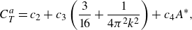 \begin{gather} C_{T}^{a} = c_{2} + c_{3}\left (\frac {3}{16} + \frac {1}{4\pi ^2k^2}\right ) + c_{4} A^*, \end{gather}
and since
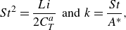 \begin{gather} St^2 = \frac {Li}{2C_{T}^a} \;\; \text{and} \;\; k=\frac {St}{A^*}, \end{gather}
we have (see Appendix A.2 for details)
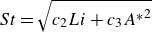 \begin{gather} St = \sqrt {c_{2} Li + c_{3} {A^*}^2} \end{gather}
and
 \begin{gather} k = \frac {1}{A^*}\sqrt {c_{2} Li + c_{3} {A^*}^2}. \end{gather}
Using the free-swimming data in § § 3.2 and 3.3, the coefficients in (3.17) and (3.18) are determined to be $c_{2} = 0.25$
and
$c_{2} = 0.25$
and $c_3 = 0.15$
, respectively, by minimising the squared residuals. Figure 13(b) compares the data of the Strouhal number with the prediction of the scaling law. It is shown that the Strouhal number of unconstrained pitching foils can be well predicted by the scaling law. Here, the comparison of the reduced frequency with its prediction is not shown since it is simply the Strouhal number divided by the dimensionless amplitude, which produces a graph showing the same agreement.
$c_3 = 0.15$
, respectively, by minimising the squared residuals. Figure 13(b) compares the data of the Strouhal number with the prediction of the scaling law. It is shown that the Strouhal number of unconstrained pitching foils can be well predicted by the scaling law. Here, the comparison of the reduced frequency with its prediction is not shown since it is simply the Strouhal number divided by the dimensionless amplitude, which produces a graph showing the same agreement.
Compiling the free-swimming data in the present study with data from previous numerical and experimental two-dimensional studies of constrained foils representing a wide Reynolds number range of $200 \leqslant Re \leqslant 59\,000$
, the coefficient in (3.9) is then determined to be
$200 \leqslant Re \leqslant 59\,000$
, the coefficient in (3.9) is then determined to be $c_{1} = 0.64$
by minimising the squared residuals. Figure 13(c) compares the ratio of the wavelength over the nominal wavelength with the scaling law prediction. The scaling law can predict the ratio of the wavelength over the nominal wavelength to within
$c_{1} = 0.64$
by minimising the squared residuals. Figure 13(c) compares the ratio of the wavelength over the nominal wavelength with the scaling law prediction. The scaling law can predict the ratio of the wavelength over the nominal wavelength to within $\pm 10\,\%$
error. Note that this
$\pm 10\,\%$
error. Note that this $10\,\%$
error also applies to the prediction of the wavelength since the wavelength is simply
$10\,\%$
error also applies to the prediction of the wavelength since the wavelength is simply $\lambda /\lambda _{0}$
multiplied by
$\lambda /\lambda _{0}$
multiplied by $c/k$
. Moreover, it is discovered that the wake wavelength can be up to
$c/k$
. Moreover, it is discovered that the wake wavelength can be up to $1.6$
times the nominal wake wavelength, indicating the inaccuracy in predicting the spacing of wake vortices with the nominal wake wavelength.
$1.6$
times the nominal wake wavelength, indicating the inaccuracy in predicting the spacing of wake vortices with the nominal wake wavelength.
From (3.3) and (3.9), the scaling law of the wake wavelength can be explicitly written as
 \begin{gather} \lambda /c = \frac {1}{k} + c_{1}St. \end{gather}
This scaling law can be used for both constrained and unconstrained studies. For unconstrained studies, in which the Strouhal number and reduced frequency are not known a priori, the scaling laws in (3.17) and (3.18) can be employed to predict the Strouhal number and reduced frequency. The present scaling law does not account for the velocities induced from leading-edge vorticies. Although leading-edge flow separation varies significantly across the Reynolds number range of $200 \leqslant Re \leqslant 59\,000$
, the good data collapse achieved by the present model shows that the wake wavelength is primarily determined by the velocities induced from trailing-edge vortices in this Reynolds number range.
$200 \leqslant Re \leqslant 59\,000$
, the good data collapse achieved by the present model shows that the wake wavelength is primarily determined by the velocities induced from trailing-edge vortices in this Reynolds number range.
3.6. Enhancing efficiency in in-line stable formations by mismatched amplitudes
In the previous sections the physics of freely swimming leader–follower foil pairs were detailed when they used identical amplitudes of motion. In this section we turn our attention to probing the potential of mismatched amplitudes, where the leader and follower use different amplitudes, to further improve the efficiency performance of the pairs while maintaining stable in-line formations. New unconstrained simulations (table 1; varying $\theta _{0,L}/\theta _{0,F}$
) and new constrained experiments (table 2) are presented in this section. We are motivated to investigate mismatched amplitudes in response to the comparison of the free-swimming data from the current study with previous constrained measurements (Kurt & Moored Reference Kurt and Moored2018).
$\theta _{0,L}/\theta _{0,F}$
) and new constrained experiments (table 2) are presented in this section. We are motivated to investigate mismatched amplitudes in response to the comparison of the free-swimming data from the current study with previous constrained measurements (Kurt & Moored Reference Kurt and Moored2018).
Table 2. Experimental variables used in the study. Experiments $1$
–
$1$
– $4$
correspond to figure 14(a,c,d,f), respectively.
$4$
correspond to figure 14(a,c,d,f), respectively.
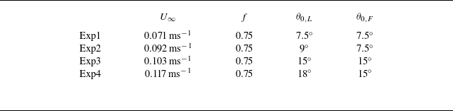
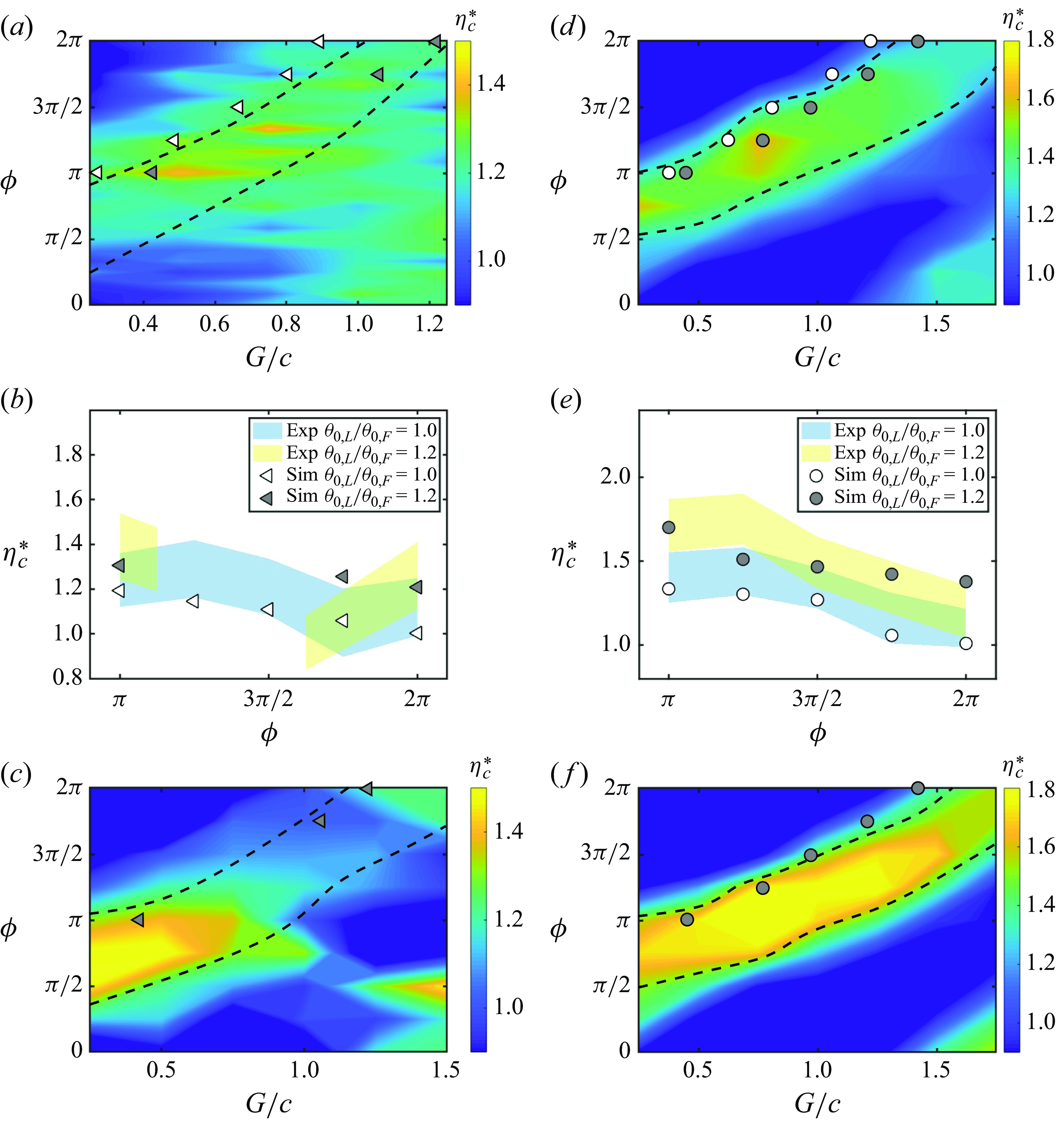
Figure 14. Further efficiency enhancement at in-line stable positions is achieved by increasing the leader’s amplitude. The efficiency contours in $(a)$
,
$(a)$
, $(c)$
,
$(c)$
, $(d)$
and
$(d)$
and $(f)$
correspond to experiments
$(f)$
correspond to experiments $1$
,
$1$
, $2$
,
$2$
, $3$
and
$3$
and $4$
in table 2, respectively. Panels
$4$
in table 2, respectively. Panels $(a)$
and
$(a)$
and $(d)$
are the experimental efficiency contours that have the same kinematics as the free-swimming simulations with
$(d)$
are the experimental efficiency contours that have the same kinematics as the free-swimming simulations with $\theta _{0,L}/\theta _{0,F}=1$
. White and grey markers represent the stable positions of the free-swimming simulations with
$\theta _{0,L}/\theta _{0,F}=1$
. White and grey markers represent the stable positions of the free-swimming simulations with $\theta _{0,L}/\theta _{0,F}=1$
and
$\theta _{0,L}/\theta _{0,F}=1$
and $1.2$
, respectively. The follower’s amplitude and the Lighthill number of the foils are fixed at
$1.2$
, respectively. The follower’s amplitude and the Lighthill number of the foils are fixed at $7.5^{\circ }$
and
$7.5^{\circ }$
and $0.18$
in
$0.18$
in $(a)$
, and fixed at
$(a)$
, and fixed at $15^{\circ }$
and
$15^{\circ }$
and $0.36$
in
$0.36$
in $(d)$
. The high-efficiency zone is outlined by dashed lines, which is defined as the region where the efficiency is at or above
$(d)$
. The high-efficiency zone is outlined by dashed lines, which is defined as the region where the efficiency is at or above $90\,\%$
of its maximum value for each phase. Panels
$90\,\%$
of its maximum value for each phase. Panels $(b)$
and
$(b)$
and $(e)$
are the normalised collective efficiency at the stable positions as a function of
$(e)$
are the normalised collective efficiency at the stable positions as a function of $\phi$
from simulations (markers) and experiments (shaded areas). The upper and lower limits of the shaded area represent the mean value plus and minus the standard deviation. Panels
$\phi$
from simulations (markers) and experiments (shaded areas). The upper and lower limits of the shaded area represent the mean value plus and minus the standard deviation. Panels $(c)$
and
$(c)$
and $(f)$
are the experimental efficiency contours that have the same kinematics as the free-swimming simulations with
$(f)$
are the experimental efficiency contours that have the same kinematics as the free-swimming simulations with $\theta _{0,L}/\theta _{0,F}=1.2$
.
$\theta _{0,L}/\theta _{0,F}=1.2$
.
To illustrate this motivation, figure 14(a) presents previous constrained experimental data (Kurt & Moored Reference Kurt and Moored2018) of the normalised efficiency as a function of $G/c$
and
$G/c$
and $\phi$
when
$\phi$
when $U=0.071\,\rm ms^-{^1}$
,
$U=0.071\,\rm ms^-{^1}$
, $f = 0.75\, \text{Hz}$
and
$f = 0.75\, \text{Hz}$
and $\theta _{0,L} = \theta _{0,F} = 7.5^{\circ }$
. A high-efficiency zone (outlined by dashed lines) where efficiency schooling benefits are maximised is observed. This zone is defined as the region where the efficiency is at or above
$\theta _{0,L} = \theta _{0,F} = 7.5^{\circ }$
. A high-efficiency zone (outlined by dashed lines) where efficiency schooling benefits are maximised is observed. This zone is defined as the region where the efficiency is at or above $90\,\%$
of its maximum value for each phase. The foil kinematics/geometry used to produce this contour are precisely the same as those used in the free-swimming simulations with
$90\,\%$
of its maximum value for each phase. The foil kinematics/geometry used to produce this contour are precisely the same as those used in the free-swimming simulations with $Li = 0.18$
and
$Li = 0.18$
and $\theta _{0}=7.5^{\circ }$
presented in § 3.2, so we directly compare the data by plotting the stable gap distances found in the free-swimming simulations (white markers) on top of the experimental contour in figure 14(a). It is discovered that the stable positions of freely swimming foils, while receiving some efficiency benefit, do not lie in the high-efficiency zone, but rather near its edge. In this way, the constrained experiments act as a map to show that there are potential additional efficiency benefits that could be unlocked if the foils’ stable gap distance were larger at a given phase difference. To achieve this, the key idea to understand is that the high efficiency benefits are driven by high follower thrust benefits (Kurt & Moored Reference Kurt and Moored2018), and if the follower is at a gap distance in the high efficiency zone then it receives too much additional thrust such that it will swim faster than the leader and reduce the gap distance until their thrusts are equilibrated. We hypothesise that by increasing the leader’s amplitude relative to the follower (or reducing the follower’s amplitude relative to the leader) the high thrust of the follower in the high efficiency zone can be matched by the leader thereby extending the stable gap distance to reside in that zone. Then the foil pair may be able to maximise its efficiency while maintaining a stable formation.
$\theta _{0}=7.5^{\circ }$
presented in § 3.2, so we directly compare the data by plotting the stable gap distances found in the free-swimming simulations (white markers) on top of the experimental contour in figure 14(a). It is discovered that the stable positions of freely swimming foils, while receiving some efficiency benefit, do not lie in the high-efficiency zone, but rather near its edge. In this way, the constrained experiments act as a map to show that there are potential additional efficiency benefits that could be unlocked if the foils’ stable gap distance were larger at a given phase difference. To achieve this, the key idea to understand is that the high efficiency benefits are driven by high follower thrust benefits (Kurt & Moored Reference Kurt and Moored2018), and if the follower is at a gap distance in the high efficiency zone then it receives too much additional thrust such that it will swim faster than the leader and reduce the gap distance until their thrusts are equilibrated. We hypothesise that by increasing the leader’s amplitude relative to the follower (or reducing the follower’s amplitude relative to the leader) the high thrust of the follower in the high efficiency zone can be matched by the leader thereby extending the stable gap distance to reside in that zone. Then the foil pair may be able to maximise its efficiency while maintaining a stable formation.
To test out this hypothesis, new free-swimming simulations were conducted where the leader-to-follower amplitude ratio is increased to $\theta _{0,L}/\theta _{0,F} = 1.2$
. We increased the amplitude ratio with an increment of
$\theta _{0,L}/\theta _{0,F} = 1.2$
. We increased the amplitude ratio with an increment of $0.1$
. The amplitude ratio of
$0.1$
. The amplitude ratio of $1.2$
provides the closest distance between the stable position and the high-efficiency zone without loosing the stable formation. It is revealed that the stable gap distances from these simulations (grey markers in figure 14
a) are indeed extended at the same phase difference, and they seem to reside in the high-efficiency zone. Note that at
$1.2$
provides the closest distance between the stable position and the high-efficiency zone without loosing the stable formation. It is revealed that the stable gap distances from these simulations (grey markers in figure 14
a) are indeed extended at the same phase difference, and they seem to reside in the high-efficiency zone. Note that at $\phi = 5\pi /4$
and
$\phi = 5\pi /4$
and $3\pi /2$
the stable formations are lost. Figure 14(b) compares the efficiency benefit calculated from the free-swimming simulations at the stable gap distances of matched and mismatched amplitudes and it is also observed that the efficiency is increased for the mismatched amplitude case, as hypothesised. In addition, the increased efficiency benefit is observed in experimental data. Despite the extended stable gap distances and the increased efficiency, it is not yet clear that the foil pair resides in the high-efficiency zone, since the contour plot in figure 14(a) represents the data from experiments on matched amplitudes of motion. When there are mismatched amplitudes the high-efficiency zone itself may be altered. Therefore, figure 14(c) presents data from new experiments of foil pairs with mismatched amplitudes (
$3\pi /2$
the stable formations are lost. Figure 14(b) compares the efficiency benefit calculated from the free-swimming simulations at the stable gap distances of matched and mismatched amplitudes and it is also observed that the efficiency is increased for the mismatched amplitude case, as hypothesised. In addition, the increased efficiency benefit is observed in experimental data. Despite the extended stable gap distances and the increased efficiency, it is not yet clear that the foil pair resides in the high-efficiency zone, since the contour plot in figure 14(a) represents the data from experiments on matched amplitudes of motion. When there are mismatched amplitudes the high-efficiency zone itself may be altered. Therefore, figure 14(c) presents data from new experiments of foil pairs with mismatched amplitudes ( $\theta _{0,L}/\theta _{0,F} = 1.2$
) with the stable gap distances of the free-swimming simulations plotted on top. Now, it is confirmed that the stable positions are indeed pushed into the high-efficiency zone when the amplitude ratio is increased to
$\theta _{0,L}/\theta _{0,F} = 1.2$
) with the stable gap distances of the free-swimming simulations plotted on top. Now, it is confirmed that the stable positions are indeed pushed into the high-efficiency zone when the amplitude ratio is increased to $\theta _{0,L}/\theta _{0,F} = 1.2$
. Surprisingly, the efficiency benefits in the zone and its neighbourhood are also increased above the case of matched amplitudes of motion.
$\theta _{0,L}/\theta _{0,F} = 1.2$
. Surprisingly, the efficiency benefits in the zone and its neighbourhood are also increased above the case of matched amplitudes of motion.
Now, the matched amplitude case presented in figure 14(a–c) ( $\theta _0 = 7.5^{\circ }$
) is not the baseline case that maximises the efficiency, so does this approach continue to increase the efficiency benefits even for the maximum efficiency baseline case, that is,
$\theta _0 = 7.5^{\circ }$
) is not the baseline case that maximises the efficiency, so does this approach continue to increase the efficiency benefits even for the maximum efficiency baseline case, that is, $\theta _{0} =15^{\circ }$
and
$\theta _{0} =15^{\circ }$
and $Li=0.36$
? To address this question, figures 14(d) and 14(f) present new constrained experimental data of the normalised efficiency for
$Li=0.36$
? To address this question, figures 14(d) and 14(f) present new constrained experimental data of the normalised efficiency for $\theta _{0,L}/\theta _{0,F} = 1$
and
$\theta _{0,L}/\theta _{0,F} = 1$
and $\theta _{0,L}/\theta _{0,F} = 1.2$
, respectively, with
$\theta _{0,L}/\theta _{0,F} = 1.2$
, respectively, with $\theta _{0,F} =15^{\circ }$
and
$\theta _{0,F} =15^{\circ }$
and $Li=0.36$
. Figure 14(e) presents the efficiency enhancement calculated from the simulations of the matched and mismatched amplitudes when the foils are freely swimming at their stable gap distances. The stable positions from the free-swimming simulations with matched and mismatched amplitudes are represented by the white and grey markers, respectively. It is discovered that the stable positions for matched amplitudes are still near the edge of the high-efficiency zone (figure 14
d) and that by increasing the leader’s amplitude from
$Li=0.36$
. Figure 14(e) presents the efficiency enhancement calculated from the simulations of the matched and mismatched amplitudes when the foils are freely swimming at their stable gap distances. The stable positions from the free-swimming simulations with matched and mismatched amplitudes are represented by the white and grey markers, respectively. It is discovered that the stable positions for matched amplitudes are still near the edge of the high-efficiency zone (figure 14
d) and that by increasing the leader’s amplitude from $\theta _0 = 15^{\circ }$
to
$\theta _0 = 15^{\circ }$
to $18^{\circ }$
it does increase the foils’ stable gap distance, and their efficiency enhancement increases from a peak baseline value of a
$18^{\circ }$
it does increase the foils’ stable gap distance, and their efficiency enhancement increases from a peak baseline value of a $33\,\%$
improvement over isolated foils to more than doubling that to a
$33\,\%$
improvement over isolated foils to more than doubling that to a $70\,\%$
improvement over isolated foils (figure 14
e). Furthermore, this increased efficiency benefit revealed by the simulations agrees well with the experimental data in figure 14(e). Despite the substantial improvement in efficiency and the increase in the foils’ stable gap distance, the foils still do not reside in the centre of the high efficiency zone (figure 14
f), but rather stay near its edge. It is observed that the zone shifts to larger gap distances at the same phase difference and the substantial efficiency enhancement over the matched amplitude case is driven by a rise in the collective efficiency levels for these mismatched amplitudes of motion. It is likely that the stable position can be tuned closer to the centre of the high-efficiency zone if we vary the amplitude ratio with a finer resolution, for example,
$70\,\%$
improvement over isolated foils (figure 14
e). Furthermore, this increased efficiency benefit revealed by the simulations agrees well with the experimental data in figure 14(e). Despite the substantial improvement in efficiency and the increase in the foils’ stable gap distance, the foils still do not reside in the centre of the high efficiency zone (figure 14
f), but rather stay near its edge. It is observed that the zone shifts to larger gap distances at the same phase difference and the substantial efficiency enhancement over the matched amplitude case is driven by a rise in the collective efficiency levels for these mismatched amplitudes of motion. It is likely that the stable position can be tuned closer to the centre of the high-efficiency zone if we vary the amplitude ratio with a finer resolution, for example, $0.01$
. However, this is beyond the scope of the article since we are showcasing tuning the amplitude ratio as an approach to bridging physics discovered in unconstrained and constrained studies of schooling, not identifying the optimum amplitude ratio.
$0.01$
. However, this is beyond the scope of the article since we are showcasing tuning the amplitude ratio as an approach to bridging physics discovered in unconstrained and constrained studies of schooling, not identifying the optimum amplitude ratio.
The constrained-foil measurements presented in figure 14, show that the general feature of high efficiency bands observed in the matched amplitude maps are reproduced in the mismatched amplitude maps regardless of changes in the efficiency levels. This is not surprising since the bands are indicative of a vortex–body impingement mechanism (Boschitsch et al. Reference Boschitsch, Dewey and Smits2014), which should not fundamentally change with mismatched amplitudes. In this way, constrained measurements of matched amplitudes can provide a map that can guide the choice of kinematics of free-swimming hydrofoils towards high efficiency. Instead of mismatched amplitudes, other strategies for tailoring stable formations could be used and investigated such as mismatched frequencies, non-sinusoidal motions and intermittent swimming. The findings in this study can aid in the design of high-efficiency biorobots that school in formation. Future work should examine data of fish schools to determine whether mismatched amplitudes is a strategy used in biology to maximise efficiency.
4. Conclusions
In this study, we simulate two pitching hydrofoils freely swimming in an in-line arrangement. It is found that self-organising in-line stable formations with efficiency benefits exist under a wide range of flow conditions defined by the phase synchrony, pitching amplitude and Lighthill number. When leading-edge flow separation is suppressed, the follower always collides into the leader and in-line stable formations cannot be formed regardless of the kinematics. Additionally, the characteristic vortex pairs above and below the follower that form during in-line schooling disappear when there is no leading-edge flow separation. Comparing constrained simulations with and without leading-edge flow separation reveals that separation acts a dynamic drag source on the follower that varies with the synchrony and gap spacing. In fact, increasing the drag of the follower by giving it a larger Lighthill number can be enough to form in-line stable formations, however, this approach only qualitatively agrees, not quantitatively to simulations and experiments where leading-edge separation on the follower is present.
From free-swimming simulations over a wide range of flow conditions typical of biology it is discovered that the nominal wake wavelength widely used in previous work does not scale the in-line stable positions, particularly for variations in the Lighthill number. The nominal wavelength can achieve a good collapse for variations in the amplitude, since the actual-to-nominal wavelength ratio is nearly constant across pitching amplitudes. However, this ratio exhibits a large variation across different Lighthill numbers, where the wake wavelength is discovered to be up to $1.6$
times the nominal wake wavelength, highlighting the inaccuracy in using the nominal wavelength to predict the spacing of wake vortices. When using the actual wake wavelength a good collapse occurs for variations in phase, amplitude and Lighthill number, and reveal a linear relationship between the phase difference and the normalised gap distance. By considering the velocity induced on a wake vortex by its neighbours, a scaling law of the wake wavelength is developed. This scaling law is applied to both unconstrained and constrained data from the current study and previous studies, showing good agreement to within
$1.6$
times the nominal wake wavelength, highlighting the inaccuracy in using the nominal wavelength to predict the spacing of wake vortices. When using the actual wake wavelength a good collapse occurs for variations in phase, amplitude and Lighthill number, and reveal a linear relationship between the phase difference and the normalised gap distance. By considering the velocity induced on a wake vortex by its neighbours, a scaling law of the wake wavelength is developed. This scaling law is applied to both unconstrained and constrained data from the current study and previous studies, showing good agreement to within $\pm 10\,\%$
error across a wide Reynolds number range of
$\pm 10\,\%$
error across a wide Reynolds number range of $200 \leqslant Re \leqslant 59\,000$
.
$200 \leqslant Re \leqslant 59\,000$
.
Considering the efficiency performance of schooling in-line foils at stable gap distances, the maximum efficiency enhancement is achieved for compact arrangements where $\lambda \lt 0.7$
and with the phase difference of
$\lambda \lt 0.7$
and with the phase difference of $\phi = \pi$
for all amplitudes except for
$\phi = \pi$
for all amplitudes except for $\theta _{0}=30^{\circ }$
where there is, in fact, an efficiency penalty compared with an isolated foil. The maximum efficiency benefit also occurs at the lowest Lighthill numbers examined of
$\theta _{0}=30^{\circ }$
where there is, in fact, an efficiency penalty compared with an isolated foil. The maximum efficiency benefit also occurs at the lowest Lighthill numbers examined of $Li = 0.09$
and at the optimal amplitude of
$Li = 0.09$
and at the optimal amplitude of $\theta _{0} = 15^{\circ }$
. In non-compact formations where
$\theta _{0} = 15^{\circ }$
. In non-compact formations where $G_{s}/\lambda \gt 0.7$
, the collective efficiency enhancement is driven by the follower’s efficiency enhancement. The follower’s efficiency is affected by leading-edge suction, a vortex pair and the reattachment of leading-edge vortex sheet. The main drivers for the power savings of the follower is the leading-edge suction force from the effective flow at the leading edge and the net force from the nearby vortex pair both acting in the direction of the foil’s motion. These forces maximally reduce the follower’s power when the vortex pair reaches the trailing edge one half-cycle after its formation. This means that the highest follower (and collective) efficiency occurs when the leader’s wake wavelength normalised by the follower’s chord is
$G_{s}/\lambda \gt 0.7$
, the collective efficiency enhancement is driven by the follower’s efficiency enhancement. The follower’s efficiency is affected by leading-edge suction, a vortex pair and the reattachment of leading-edge vortex sheet. The main drivers for the power savings of the follower is the leading-edge suction force from the effective flow at the leading edge and the net force from the nearby vortex pair both acting in the direction of the foil’s motion. These forces maximally reduce the follower’s power when the vortex pair reaches the trailing edge one half-cycle after its formation. This means that the highest follower (and collective) efficiency occurs when the leader’s wake wavelength normalised by the follower’s chord is $\lambda /c \approx 2$
, which is corroborated with the simulation data.
$\lambda /c \approx 2$
, which is corroborated with the simulation data.
By using measurements of matched amplitude constrained foils as a guide, it was hypothesised that by increasing the amplitude of the leader relative to the follower – using mismatched amplitudes – the pair of foils could self-organise with a gap spacing in a zone of high efficiency. New constrained experiments and free-swimming simulations confirmed this hypothesis and showed that by using matched amplitudes the peak efficiency of the foil pair could increase by 33 % over isolated foils while using mismatched amplitudes could more than double that to a 70 % increase over isolated foils. This occurs for mismatched amplitudes by (i) increasing the stable gap distance between foils such that they are pushed into a high-efficiency zone, and (ii) by raising the level of efficiency in these zones. This study not only presents a way to tailor in-line stable formations towards high efficiency via mismatched amplitudes, but also bridges the gap between constrained and unconstrained studies. It is shown that constrained foil measurements can be used as a map of the potential benefits of schooling, which can guide the choice of kinematics of free-swimming hydrofoils towards high efficiency. The findings and scaling laws in this article are for pitching foils. These findings and scaling laws can be different for other foil kinematics, such as heaving and combined pitching and heaving, as different kinematics lead to different leading-edge and bound vortices. In addition, a Reynolds number or foil shape different from those used in the present study can give different leading-edge separation and lead to different results. Furthermore, future efforts to conduct a comprehensive parametric study to investigate schooling with mismatched amplitudes at different amplitude ratios and amplitudes and examine the performance of individuals in the school would help tune stable positions closer to the high-efficiency zone.
Funding
This work was supported by the Office of Naval Research under Program Director Dr R. Brizzolara on MURI grant no. N00014-22-1-2616.
Declaration of interests
The authors report no conflict of interest.
Appendix A. Derivation of scaling laws
A.1. Scaling law for the induced velocity
 \begin{gather} U_{i} = \frac {\Gamma A}{\pi \left (\frac {(U+U_{i})^2}{4f^2} + A^2\right )}. \end{gather}
After non-dimensionalisation, (A1) becomes
 \begin{gather} U^*_{i} = \frac {\Gamma ^*}{\pi A^{*} U\left (\frac {(1+U^*_{i})^2}{4St^2} + 1\right )}, \end{gather}
where $\Gamma ^*$
is the non-dimensional wake circulation,
$\Gamma ^*$
is the non-dimensional wake circulation, $\Gamma ^* = {\Gamma }/{Uc}$
. After organisation (A2) becomes
$\Gamma ^* = {\Gamma }/{Uc}$
. After organisation (A2) becomes
 \begin{gather} {U^*_{i}}^3 + 2{U^*_{i}}^2 + U^*_{i}(1+4St^2) = \frac {4St^2\Gamma ^*}{\pi A^*}. \end{gather}
Since $U^*_{i}$
and
$U^*_{i}$
and $St$
are less than
$St$
are less than $1$
, we neglect the terms of
$1$
, we neglect the terms of ${U^*_{i}}^3$
and
${U^*_{i}}^3$
and $U^*_{i}St^2$
in (A3) for simplification, which gives
$U^*_{i}St^2$
in (A3) for simplification, which gives
 \begin{gather} 2{U^*_{i}}^2 + U^*_{i} = \frac {4St^2\Gamma ^*}{\pi A^*}. \end{gather}
Solving (A4) gives
 \begin{gather} U^*_{i} = -\frac {1}{4} + \frac {1}{4}\sqrt {1+\frac {32St^2\Gamma ^*}{\pi A^*}}. \end{gather}
Following Han et al. (Reference Han, Zhong, Mivehchi, Quinn and Moored2024) and Moored & Quinn (Reference Moored and Quinn2019), we have
 \begin{gather} \Gamma ^* \propto \Gamma ^*_{0}\frac {k^*}{1+k^*}, \end{gather}
with
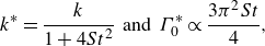 \begin{gather} k^* = \frac {k}{1+4St^2} \;\; \text{and} \;\;\Gamma ^*_{0} \propto \frac {3\pi ^2 St}{4}, \end{gather}
where $\Gamma ^*_{0}$
is the non-dimensional quasisteady circulation of a foil pitching about its leading edge. Then we have
$\Gamma ^*_{0}$
is the non-dimensional quasisteady circulation of a foil pitching about its leading edge. Then we have
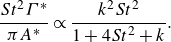 \begin{gather} \frac {St^2\Gamma ^*}{\pi A^*} \propto \frac {k^2St^2}{1+4St^2+k}. \end{gather}
So (A5) becomes
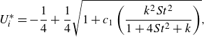 \begin{gather} U^*_{i} = -\frac {1}{4} + \frac {1}{4}\sqrt {1+c_1 \left (\frac { k^2St^2}{ 1+4St^2+k}\right )}, \end{gather}
where $c_{1}$
needs to be determined. Since the last term in (A9) is much larger than the other terms, (A9) can be approximated as
$c_{1}$
needs to be determined. Since the last term in (A9) is much larger than the other terms, (A9) can be approximated as
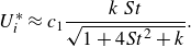 \begin{gather} U^*_{i} \approx c_{1}\frac { k\, St}{ \sqrt {1+4St^2+k}}. \end{gather}
Furthermore, since the variation of the denominator is much less than the numerator in (A10), we approximate the denominator as a constant and simplify the equation, which gives
 \begin{gather} U^*_{i} = c_{1}\, k\, St. \end{gather}
A.2. Scaling law for the Strouhal number and reduced frequency of unconstrained foils
From (3.15) and (3.16), we have
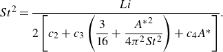 \begin{gather} St^2 = \frac {Li}{2\left [c_{2} + c_{3}\left ( \dfrac {3}{16} + \dfrac {{A^*}^2}{4\pi ^2 St^2} \right ) + c_{4} A^*\right ]} . \end{gather}
After organisation we have
 \begin{gather} St^2 \left (c_{2} + \frac {3}{16} c_{3} + c_{4} A^* \right ) = \frac {Li}{2} - \frac {c_{3} {A^*}^2}{4\pi ^2}. \end{gather}
Therefore, the Strouhal number is calculated as
 \begin{gather} St = \sqrt { \frac {\dfrac {Li}{2} - \dfrac {c_3 {A^*}^2}{4 \pi ^2}}{c_{2} + \dfrac {3}{16}c_{3} + c_{4} A^*} }. \end{gather}
Because the variation of the denominator is much less than the numerator in (A14), we approximate the denominator as a constant and simplify (A14) to
 \begin{gather} St = \sqrt {c_{2} Li + c_{3} {A^*}^2}. \end{gather}
In addition, the reduced frequency is calculated as
 \begin{gather} k = \frac {St}{A^*} = \frac {1}{A^*}\sqrt {c_{2} Li + c_{3} {A^*}^2}. \end{gather}
Appendix B. Performance variation with a finer resolution
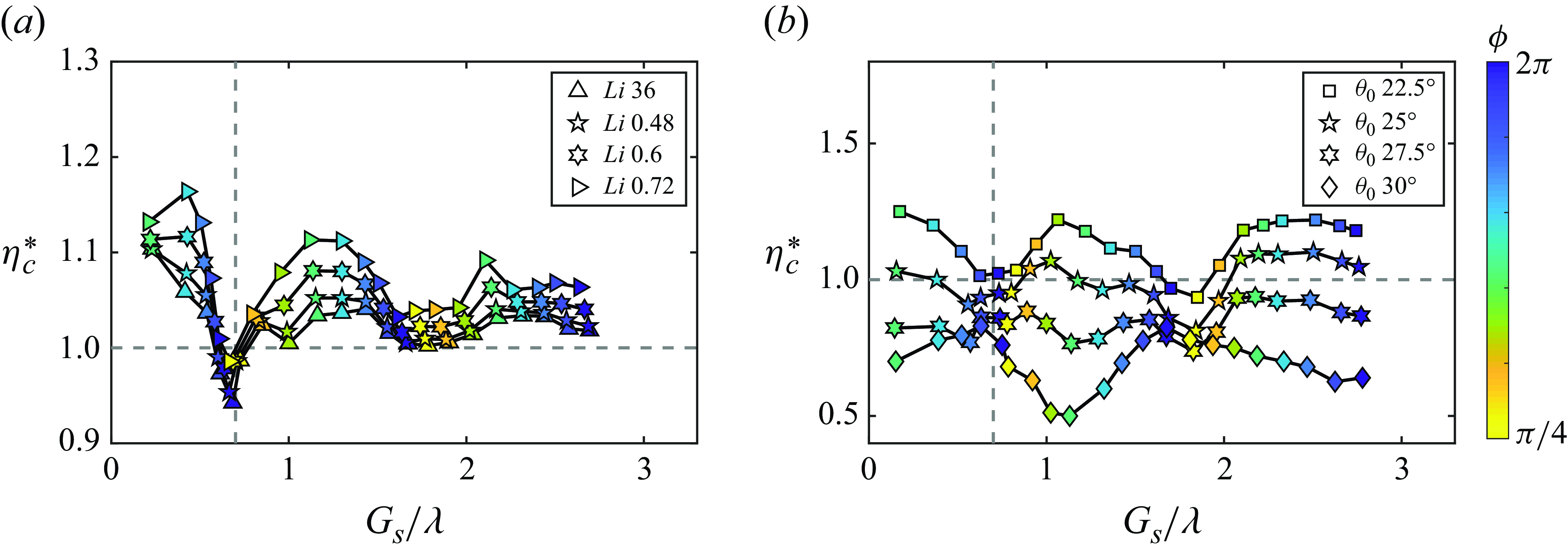
Figure 15. Normalised collective efficiency as a function of the normalised gap distance for $(a)$
varying
$(a)$
varying $Li$
from
$Li$
from $Li = 0.36$
to
$Li = 0.36$
to $0.72$
with
$0.72$
with $\theta _{0}$
fixed at
$\theta _{0}$
fixed at $\theta _{0} = 7.5^{\circ }$
and
$\theta _{0} = 7.5^{\circ }$
and $(b)$
varying
$(b)$
varying $\theta _{0}$
from
$\theta _{0}$
from $\theta _{0} = 22.5^{\circ }$
to
$\theta _{0} = 22.5^{\circ }$
to $30^{\circ }$
with
$30^{\circ }$
with $Li$
fixed at
$Li$
fixed at $Li = 0.36$
. The grey vertical dashed line represents
$Li = 0.36$
. The grey vertical dashed line represents $G_s/\lambda =0.7$
.
$G_s/\lambda =0.7$
.
As shown in figure 8(d), when $\theta _{0}$
is fixed at
$\theta _{0}$
is fixed at $7.5^{\circ }$
, the maximum collective efficiency enhancement decreases with increasing
$7.5^{\circ }$
, the maximum collective efficiency enhancement decreases with increasing $Li$
from
$Li$
from $Li = 0.09$
to
$Li = 0.09$
to $0.36$
and then increases with further increases in
$0.36$
and then increases with further increases in $Li$
from
$Li$
from $Li = 0.36$
to
$Li = 0.36$
to $0.72$
. To better resolve this non-monotonic trend, we present additional simulations at
$0.72$
. To better resolve this non-monotonic trend, we present additional simulations at $Li = 0.48$
and
$Li = 0.48$
and $Li = 0.6$
in figure 15(a). For the additional data, the maximum efficiency enhancement is still achieved for compact arrangements with
$Li = 0.6$
in figure 15(a). For the additional data, the maximum efficiency enhancement is still achieved for compact arrangements with $G_{s}/\lambda \lt 0.7$
. As
$G_{s}/\lambda \lt 0.7$
. As $Li$
increases from
$Li$
increases from $Li=0.36$
to
$Li=0.36$
to $0.72$
, the maximum collective efficiency enhancement increases, which demonstrates that
$0.72$
, the maximum collective efficiency enhancement increases, which demonstrates that $Li=0.36$
is the transitioning point for the non-monotonic trend. In addition, the phase where the maximum collective efficiency enhancement is achieved shifts from
$Li=0.36$
is the transitioning point for the non-monotonic trend. In addition, the phase where the maximum collective efficiency enhancement is achieved shifts from $\pi$
to
$\pi$
to $5\pi /4$
when
$5\pi /4$
when $Li$
increases from
$Li$
increases from $Li=0.36$
to
$Li=0.36$
to $0.72$
. Furthermore, the two additional cases follow the same trend as the cases in figure 8(d) that the collective efficiency has successive peaks that have gap distances one wavelength apart, and nearly all of the peaks in efficiency occur for
$0.72$
. Furthermore, the two additional cases follow the same trend as the cases in figure 8(d) that the collective efficiency has successive peaks that have gap distances one wavelength apart, and nearly all of the peaks in efficiency occur for $\phi \approx \pi$
while nearly all of the troughs occur for
$\phi \approx \pi$
while nearly all of the troughs occur for $\phi \approx 0$
.
$\phi \approx 0$
.
Figure 15(b) presents additional simulations at $\theta _{0} = 25^{\circ }$
and
$\theta _{0} = 25^{\circ }$
and $\theta _{0} = 27.5^{\circ }$
with
$\theta _{0} = 27.5^{\circ }$
with $Li$
fixed at
$Li$
fixed at $Li = 0.36$
to better resolve the considerable performance drop when
$Li = 0.36$
to better resolve the considerable performance drop when $\theta _{0}$
increases from
$\theta _{0}$
increases from $22.5^{\circ }$
to
$22.5^{\circ }$
to $30^{\circ }$
in figure 9(d). At
$30^{\circ }$
in figure 9(d). At $\theta _{0} = 22.5^{\circ }$
, peaks in the collective efficiency enhancement occur at
$\theta _{0} = 22.5^{\circ }$
, peaks in the collective efficiency enhancement occur at $\phi \approx \pi$
, and troughs occurs at
$\phi \approx \pi$
, and troughs occurs at $\phi \approx 0$
. When
$\phi \approx 0$
. When $\theta _{0}$
increases from
$\theta _{0}$
increases from $\theta _{0} = 22.5^{\circ }$
to
$\theta _{0} = 22.5^{\circ }$
to $30^{\circ }$
, the collective efficiency enhancement decreases from above
$30^{\circ }$
, the collective efficiency enhancement decreases from above $1$
to below
$1$
to below $1$
, showing efficiency penalty. The amplitude of
$1$
, showing efficiency penalty. The amplitude of $\theta _{0} = 25^{\circ }$
is the transitioning point, whose collective efficiency enhancement oscillates about
$\theta _{0} = 25^{\circ }$
is the transitioning point, whose collective efficiency enhancement oscillates about $1$
. Furthermore, the collective efficiency enhancement at
$1$
. Furthermore, the collective efficiency enhancement at $\phi \approx \pi$
decreases faster than that at
$\phi \approx \pi$
decreases faster than that at $\phi \approx 0$
, which results in the flip of the locations of peaks and troughs at
$\phi \approx 0$
, which results in the flip of the locations of peaks and troughs at $\theta _{0}=30^{\circ }$
.
$\theta _{0}=30^{\circ }$
.


 Open access