


1. Introduction
Numerical simulations of fluid flows are carried out with ever growing spatial resolution. In contrast, observational data are limited to relatively coarse sensor measurements. This dichotomy inhibits efficient integration of experimental data with existing high-fidelity computational methods to enable detailed and accurate flow analysis or prediction.
As we review in § 1.1, several methods have been developed to address this disconnect. In particular, flow reconstruction methods seek to leverage offline high-resolution simulations to estimate the entire flow field from coarse online observations. All existing methods vectorize the simulation data by stacking different spatial dimensions on top of each other. Vectorization is convenient since it enables one to use familiar linear algebra techniques. However, this approach inevitably leads to loss of information encoded in the inherent multidimensional structure of the flow.
Here, we propose a tensor-based sensor placement and flow reconstruction method which retains and exploits the multidimensional structure of the flow. Our method significantly increases the accuracy of the reconstruction compared with similar vectorized methods. We quantify this accuracy by deriving an upper bound for the reconstruction error and show that the resulting approximation exactly interpolates the flow at the sensor locations (assuming the measurements are noise free). Additionally, the proposed method has a smaller memory footprint compared with the similar vectorized methods, and is scalable to large data sets using randomized techniques. We demonstrate the efficacy of our method on three examples: direct numerical simulation of a turbulent Kolmogorov flow, in situ and satellite sea surface temperature (SST) data and three-dimensional (3-D) unsteady simulated flow around a marine research vessel. We emphasize that our focus here is only on flow reconstruction and not temporal prediction; nonetheless, the reconstructed flow can be subsequently used as input to high-fidelity or reduced-order predictive models.
1.1. Related work
Due to the broad applications of flow estimation from sparse measurements, there is an expansive body of work on this subject (see Callaham, Maeda & Brunton (Reference Callaham, Maeda and Brunton2019) for a thorough review). Here, we focus on the so-called library-based methods. These methods seek to reconstruct the flow field by leveraging the sparse observational measurements to interpolate a pre-computed data library comprising high-fidelity numerical simulations. More specifically, consider a scalar quantity  $g(\boldsymbol{x},t)$ which we would like to reconstruct from its spatially sparse measurements. For instance, this quantity may be a velocity component, a vorticity component, pressure or temperature. The data library is a matrix $\varPhi \in \mathbb {R}^{N\times T}$ whose columns are formed from vectorized high-resolution simulations. Here, $N$ denotes the number of collocation points used in the simulations. The columns of $\varPhi$ may coincide with the quantity of interest $g$ or be derived from this quantity, e.g. through proper orthogonal decomposition (POD) or dynamic mode decomposition (DMD). The observational data $\boldsymbol{y}\in \mathbb {R}^r$ form a vector containing $r$ measurements of the quantity $g$ at a particular time. Library-based methods seek to find a map $F:\mathbb {R}^{N\times T}\times \mathbb {R}^r\to \mathbb {R}^N$ such that $\boldsymbol{g} \simeq F(\varPhi,\boldsymbol{y})$. Here, $\boldsymbol{g}\in \mathbb {R}^N$ is a vector obtained by stacking the quantity of interest $g(\boldsymbol{x},t)$ at the collocation points.
Library-based methods differ in their choice of the data matrix  $\varPhi$ and the methodology for finding the map $F$. A common choice for the columns of the data matrix is the POD modes (Bui-Thanh, Damodaran & Willcox Reference Bui-Thanh, Damodaran and Willcox2004; Willcox Reference Willcox2006), although DMD modes (Kramer et al. Reference Kramer, Grover, Boufounos, Nabi and Benosman2017; Dang, Nasreen & Zhang Reference Dang, Nasreen and Zhang2021) and flow snapshots (Clark, Brunton & Kutz Reference Clark, Brunton and Kutz2021) have also been used. Bui-Thanh et al. (Reference Bui-Thanh, Damodaran and Willcox2004) use the gappy POD algorithm of Everson & Sirovich (Reference Everson and Sirovich1995) to reconstruct the flow. They obtain the map $F$ by solving a least squares problem which seeks to minimize the discrepancy between the observations $\boldsymbol{y}$ and the reconstructed flow $F(\varPhi,\boldsymbol{y})$ at the sensor locations (also see Willcox Reference Willcox2006).
The discrete empirical interpolation method (DEIM) takes a similar approach, but the map  $F$ is a suitable oblique projection on the linear subspace spanned by the columns of $\varPhi$. DEIM was first developed by Chaturantabut & Sorensen (Reference Chaturantabut and Sorensen2010) for efficient reduced-order modelling of nonlinear systems and was later used for flow reconstruction (Drmač & Gugercin Reference Drmač and Gugercin2016; Wang et al. Reference Wang, Ding, Hu, Fang, Navon and Lin2021). Several subsequent modifications to DEIM have been proposed, e.g. to lower its computational cost (Peherstorfer et al. Reference Peherstorfer, Butnaru, Willcox and Bungartz2014) and to generalize it for use with weighted inner products (Drmač & Saibaba Reference Drmač and Saibaba2018).
It is well known that both gappy POD and DEIM suffer from overfitting (Peherstorfer, Drmač & Gugercin Reference Peherstorfer, Drmač and Gugercin2020). Consequently, if the sensor data  $\boldsymbol{y}$ are corrupted by significant observational noise, the reconstruction error will be large. Callaham et al. (Reference Callaham, Maeda and Brunton2019) use sparsity promoting techniques from image recognition to overcome this problem (also see Chu & Farazmand Reference Chu and Farazmand2021). Their reconstruction map $F$ is obtained by solving a sparsity-promoting optimization problem with the constraint that the reconstruction error is below a prescribed threshold. The resulting method is robust to observational noise. However, unlike gappy POD and DEIM, the reconstruction map $F$ cannot be expressed explicitly in terms of the training data $\varPhi$.
Yet another flow reconstruction method is to represent the map  $F$ with a neural network which is trained using the observations $\boldsymbol{y}$ and the data matrix $\varPhi$. For instance, Yu & Hesthaven (Reference Yu and Hesthaven2019) use an autoencoder to represent the reconstruction map $F$ (also see Carlberg et al. Reference Carlberg, Jameson, Kochenderfer, Morton, Peng and Witherden2019; Fukami, Fukagata & Taira Reference Fukami, Fukagata and Taira2019; Erichson et al. Reference Erichson, Mathelin, Yao, Brunton, Mahoney and Kutz2020). Unlike DEIM, where the reconstruction map $F$ is a linear combination of modes, neural networks can construct nonlinear maps from the observations $\boldsymbol{y}$ and the library $\varPhi$. These machine learning methods have shown great promise; however, the resulting reconstructions are not explicit, or even interpretable, since they are only available as a complex neural network.
With the notable exception of convolutional neural networks (Carlberg et al. Reference Carlberg, Jameson, Kochenderfer, Morton, Peng and Witherden2019; Fukami et al. Reference Fukami, Fukagata and Taira2019), almost all existing methods treat the data as a vector by stacking different spatial dimensions on top of each other. This inevitably leads to loss of information encoded in the inherent multidimensionality of the flow. Here, we propose a tensor-based method which retains and exploits this multidimensional structure. Our method is similar to the tensor-based DEIM which was recently proposed by Kirsten (Reference Kirsten2022) for model reduction; but we use it for flow reconstructions which is the focus of this paper. Numerical experiments show that the resulting reconstructions are more accurate compared with similar vectorized methods, because of our method's ability to capture and exploit the inherent multidimensional nature of the data. The computational cost of our tensor-based method is comparable to the vectorized methods and can be further accelerated using randomized methods. Furthermore, the tensor-based method requires much less storage compared with the vectorized methods. This is especially important in large-scale 3-D flows where the storage costs can be substantial (Gelss et al. Reference Gelss, Klus, Eisert and Schütte2019). Although our method is a tensorized version of DEIM, a similar tensor-based approach can be applied to other flow reconstruction methods such as gappy POD, sparsity-promoting methods and autoencoders.
2. Tensor-based flow reconstruction
2.1. Set-up and preliminaries
Let  $g(\boldsymbol{x},t)$ denote the quantity of interest at time $t$ that we would like to reconstruct. This quantity may, for instance, be a velocity component, a vorticity component, pressure or temperature. The spatial variable is denoted by $\boldsymbol{x}\in \varOmega \subset \mathbb {R}^d$, where $\varOmega$ is the flow domain with $d=2$ or $d=3$ for 2-D and 3-D flows, respectively. In numerical simulations, the quantity of interest $g$ is discretized on a spatial grid of size $N_1\times N_2\times \cdots \times N_d$ and saved as a tensor $\boldsymbol{\mathcal{G}}\in \mathbb {R}^{N_1\times \cdots \times N_d}$.
We denote entries of  $\boldsymbol{\mathcal{G}}$ by $g_{i_1,\ldots,i_d}$ where $1 \leq i_n \leq N_n$ and $1 \leq n \leq d$. There are $d$ different matrix unfoldings of $\boldsymbol{\mathcal{G}}$, also called matricizations, which we denote by $\boldsymbol {G}_{(n)} \in \mathbb {R}^{N_n \times (\prod _{j \neq n} N_j)}$. The mode- $n$ product of a tensor $\boldsymbol {\mathcal {G}}$ with a matrix $\boldsymbol {M} \in \mathbb {R}^{R \times N_n}$ is denoted as $\boldsymbol {\mathcal {Y}} = \boldsymbol {\mathcal {G}} \times _n \boldsymbol {M}$ with entries
 \begin{equation} y_{i_i,\ldots, j,\ldots, i_N} = \sum_{k=1}^R g_{i_1,\ldots,k,\ldots,i_N}m_{jk}\quad 1 \leq j \leq R. \end{equation}
 In terms of matrix unfoldings, it can be expressed as  $\boldsymbol {Y}_{(n)} = \boldsymbol {M} \boldsymbol {G}_{(n)}$. For matrices $\boldsymbol {A}$ and $\boldsymbol {B}$ of compatible dimensions $\boldsymbol {\mathcal {G}} \times _m \boldsymbol {A} \times _n \boldsymbol {B} = \boldsymbol {\mathcal {G}} \times _n \boldsymbol {B} \times _m \boldsymbol {A}$ if $m \neq n$ and $\boldsymbol {\mathcal {G}} \times _n \boldsymbol {A} \times _n \boldsymbol {B} = \boldsymbol {\mathcal {G}} \times _n \boldsymbol {BA}$. Associated with every tensor $\boldsymbol {\mathcal {G}}$ is a multirank $(R_1,\ldots,R_d)$ where $R_n = \text {rank}(\boldsymbol {G}_{(n)})$. The Frobenius norm of a tensor is $\|\boldsymbol {\mathcal {G}}\|_F^2 = \sum _{i_1,\ldots,i_d}g_{i_1,\ldots,i_d}^2$. We refer to Kolda & Bader (Reference Kolda and Bader2009) for a detailed review of tensor operations.
2.2. Vectorized POD-DEIM
We first review the vectorized form of POD-DEIM from which our tensor-based method is derived. We refer to this method as vector-DEIM, for short. In vector-DEIM approach for sensor placement (Clark et al. Reference Clark, Askham, Brunton and Kutz2018; Manohar et al. Reference Manohar, Brunton, Kutz and Brunton2018), the training data are constructed as the snapshot matrix,  $\boldsymbol {G} = [\boldsymbol {g}_1\enspace \cdots \enspace \boldsymbol {g}_T] \in \mathbb {R}^{N \times T}$, where each column $\boldsymbol {g}_j \in \mathbb {R}^N$ represents a vectorized snapshot of the quantity of interest $g(\boldsymbol{x},t_j)$. We assume that the vectors are centred, which means that the mean is subtracted from each column. We would like to pick $r \leq \min \{N,T\}$ number of sensor locations at which to collect data (see figure 1).

Figure 1. Schematic representation of the workflow in vector-DEIM and tensor-DEIM. The horizontal and vertical black bars mark the entries that are used for sensor placement (black circles). In tensor-DEIM, some sensors may fall on land and will be discarded (e.g. the one marked by the red circle).
We first compute the truncated singular value decomposition (SVD)  $\boldsymbol {G} \approx \boldsymbol {U}_r \boldsymbol{\varSigma} _r \boldsymbol{V}_r^\top$, where the columns of $\boldsymbol {U}_r\in \mathbb {R}^{N\times r}$ coincide with the POD modes. In DEIM, we compute the column-pivoted QR factorization (Golub & Van Loan Reference Golub and Van Loan2013, § 5.4.2) of $\boldsymbol {U}_r$; that is, we compute $\boldsymbol {U}_r^\top [\boldsymbol {P}_1 \enspace \boldsymbol {P}_2] = \boldsymbol {Q}_1 [\boldsymbol {R}_{11}\enspace \boldsymbol {R}_{12}]$, where $\boldsymbol {Q}_1 \in \mathbb {R}^{r\times r}$ is orthogonal, $\boldsymbol {R}_{11} \in \mathbb {R}^{r\times r}$ is upper triangular and $\boldsymbol {R}_{12} \in \mathbb {R}^{r\times N}$. The matrix $\boldsymbol {P} = [\boldsymbol {P}_1 \enspace \boldsymbol {P}_2]$ is a permutation matrix. Suppose we have $\boldsymbol {P}_1 = [\boldsymbol {I}(:,{i_1}) \enspace \cdots \enspace \boldsymbol {I}(:,i_r)]$, where $\boldsymbol{I}$ is the $N\times N$ identity matrix. Then, the matrix $\boldsymbol {P}_1 \in \mathbb {R}^{N\times r}$ contains columns from the identity matrix indexed by the set $\mathcal {I} = \{i_1,\ldots, i_r\}$. The spatial locations corresponding to the index set $\mathcal {I}$ are used as the optimal sensor locations, which may not be uniquely determined.
Suppose we want to reconstruct the flow field corresponding to the vector  $\boldsymbol {f} \in \mathbb {R}^N$. We collect measurements at the indices corresponding to $\mathcal {I}$, given by the vector $\boldsymbol {f}(\mathcal {I})$. In other words, $\boldsymbol {f}(\mathcal {I})$ is the available sensor measurements of the vector $\boldsymbol {f}$. To reconstruct the full flow field $\boldsymbol {f}$, we use the approximation
 \begin{equation} \boldsymbol{f} \approx \boldsymbol{U}_r \boldsymbol{U}_r(\mathcal{I},:)^{{-}1}\boldsymbol{f}(\mathcal{I}) = \boldsymbol{U}_r(\boldsymbol{S}^\top\boldsymbol{U}_r)^{{-}1}\boldsymbol{S}^\top\boldsymbol{f}, \end{equation}
where  $\boldsymbol {S} =\boldsymbol {P}_1$. This approximation provides insight into how the indices $\mathcal {I}$ should be selected. Since $\boldsymbol {U}_r$ has rank $r$, it is guaranteed to have $r$ linearly independent rows and $\boldsymbol {S}^\top \boldsymbol {P}_1$ is invertible. The index set $\mathcal {I}$ is chosen in such a way that the corresponding rows of $\boldsymbol {U}_r$ are well conditioned.
The error in the training set takes the form
 \begin{equation} \| \boldsymbol{G} - \boldsymbol{U}_r \boldsymbol{U}_r(\mathcal{I},:)^{{-}1} \boldsymbol{G}(\mathcal{I},:)\|_F \leq \|( \boldsymbol{S}^\top \boldsymbol{U}_r)^{{-}1}\|_2 \left(\sum_{j=r+1}^{\min\{N,T\}}\sigma_{j}^2 (\boldsymbol{G}) \right)^{1/2}, \end{equation}
where  $\sigma _j(\boldsymbol {G})$ represents the singular values of $\boldsymbol {G}$. In the above expression for the error, $(\sum _{j=r+1}^{\min \{N,T\}}\sigma _{j}^2 (\boldsymbol {G}) )^{1/2} = \|\boldsymbol {G} - \boldsymbol {U}_r\boldsymbol {U}_r^\top \boldsymbol {G}\|_F$ represents the error in the POD approximation due to the truncated singular values, which is amplified by the factor $\|( \boldsymbol {S}^\top \boldsymbol {U}_r)^{-1}\|_2$ which arises due to the DEIM approximation. The error in the test data set can be obtained using Lemma 3.2 of Chaturantabut & Sorensen (Reference Chaturantabut and Sorensen2010).
2.3. Tensor-based POD-DEIM
In vector-DEIM, the snapshots are treated as vectors meaning that the inherent multidimensional structure of the flow is lost. In order to fully exploit this multidimensional structure, we use tensor-based methods. We refer to the resulting tensorized version of POD-DEIM as tensor-DEIM, for short. We consider the collection of snapshots in the form of a tensor  $\boldsymbol {\mathcal {G}} \in \mathbb {R}^{N_1 \times \cdots \times N_d \times T }$ of order $d+1$, where $d$ represents the number of spatial dimensions and $\prod _{j=1}^dN_j = N$ is the total number of grid points (see figure 1). With this notation, the snapshot matrix $\boldsymbol {G}$ in vector-DEIM can be expressed as $\boldsymbol {G}_{(d+1)}^\top$; that is the transpose of the mode- $(d+1)$ unfolding.
Suppose we wanted to collect data at  $r = \prod _{n=1}^d r_n$ sensor locations. In tensor-DEIM, we first compute the truncated SVD of the first $d$ mode unfoldings. That is, we compute $\boldsymbol {G}_{(n)} \approx \boldsymbol {U}_r^{(n)} \boldsymbol{\varSigma} _r^{(n)} (\boldsymbol{V}_r^{(n)})^\top$ where $\boldsymbol {U}_r^{(n)} \in \mathbb {R}^{N_n \times r_n}$. For ease of notation, we define $\boldsymbol{\varPhi}_n := \boldsymbol{U}_r^{(n)}$. Next, we compute the column-pivoted QR factorization of $\boldsymbol{\varPhi}_n$ as
 \begin{equation} \boldsymbol{\varPhi}_n^\top\begin{bmatrix} \boldsymbol{P}_1^{(n)} & \boldsymbol{P}_2^{(n)} \end{bmatrix} = \boldsymbol{Q}_{1}^{(n)} \begin{bmatrix} \boldsymbol{R}_{11}^{(n)} & \boldsymbol{R}_{12}^{(n)} \end{bmatrix} \quad 1 \leq n \leq d. \end{equation}
Here,  $[\boldsymbol {P}_1^{(n)}\enspace \boldsymbol {P}_2^{(n)}]$ is a permutation matrix. Once again, for ease of notation, we set $\boldsymbol {S}_n := \boldsymbol {P}_1^{(n)}$; this matrix contains the columns from the $N_n \times N_n$ identity matrix corresponding to the indices $\mathcal {I}_n = \{i_1^{(n)}, \ldots, i_{r_n}^{(n)}\}$. Then the sensors can be placed at the spatial locations corresponding to the index set $\mathcal {I}_1 \times \cdots \times \mathcal {I}_d$. Note that when $d=1$ tensor-DEIM reduces to vector-DEIM.
Given new data  $\boldsymbol {\mathcal {F}} \in \mathbb {R}^{N_1 \times \cdots \times N_d}$, such that $\boldsymbol {f} = \text {vec}(\boldsymbol {\mathcal {F}})$, we only need to collect data at the indices corresponding to $\mathcal {I}_1 \times \cdots \times \mathcal {I}_d$, that is, we measure $\boldsymbol {\mathcal {F}}(\mathcal {I}_1,\ldots,\mathcal {I}_d)$. To reconstruct the flow field from these measurements, we compute
 \begin{equation} \boldsymbol{\mathcal{F}} \approx \boldsymbol{\mathcal{F}}(\mathcal{I}_1,\ldots,\mathcal{I}_d) \times_{n=1}^d \boldsymbol{\varPhi}_n (\boldsymbol{S}_n^\top\boldsymbol{\varPhi}_n)^{{-}1} = \boldsymbol{\mathcal{F}} \times_{n=1}^d \boldsymbol{\varPhi}_n (\boldsymbol{S}_n^\top\boldsymbol{\varPhi}_n)^{{-}1}\boldsymbol{S}_n^\top. \end{equation}
The second expression, while equivalent to the first, is more convenient for the forthcoming error analysis. The approximation just derived satisfies the interpolation property; that is, the approximation exactly matches the function  $\boldsymbol {\mathcal {F}}$ at the sensor locations assuming the measurements are noise free. To see this, denote $\boldsymbol {\mathcal {F}}_{TDEIM} := \boldsymbol {\mathcal {F}} \times _{n=1}^d \boldsymbol{\varPhi}_n (\boldsymbol{S}_n^\top \boldsymbol{\varPhi}_n)^{-1}\boldsymbol{S}_n^\top$. Then
 \begin{align} \boldsymbol{\mathcal{F}}_{TDEIM}(\mathcal{I}_1,\ldots,\mathcal{I}_d) &= \boldsymbol{\mathcal{F}}_{TDEIM} \times_{n=1}^d \boldsymbol{S}_n^\top = \boldsymbol{\mathcal{F}} \times_{n=1}^d \boldsymbol{S}_n^\top \boldsymbol{\varPhi}_n (\boldsymbol{S}_n^\top\boldsymbol{\varPhi}_n)^{{-}1}\boldsymbol{S}_n^\top \nonumber\\ &= \boldsymbol{\mathcal{F}} \times_{n=1}^d \boldsymbol{S}_n^\top = \boldsymbol{\mathcal{F}}(\mathcal{I}_1,\ldots,\mathcal{I}_d). \end{align}
The following theorem provides an expression for the error in the approximation as applied to the training data set.
Theorem 1 Suppose  $\boldsymbol{\varPhi} _n \in \mathbb {R}^{N_n\times r_n}$ is computed from the truncated rank- $r_n$ SVD of the mode unfolding $\boldsymbol {G}_{(n)}$ and $\boldsymbol {S}_n$ is obtained by computing column-pivoted QR of $\boldsymbol{\varPhi} _n^\top$ such that $\boldsymbol {S}_n^\top \boldsymbol{\varPhi} _n$ is invertible for $1 \leq n \leq d$. Define $\boldsymbol{\varPi}_n := \boldsymbol{\varPhi} _n (\boldsymbol{S}_n^\top \boldsymbol{\varPhi} _n)^{-1}\boldsymbol{S}_n^\top$ and assume $1 \leq r_n < N_n$ for $1 \leq n \leq d$. Then
 \begin{equation} \|\boldsymbol{\mathcal{G}} - \boldsymbol{\mathcal{G}} \times_{n=1}^d \boldsymbol{\varPi}_n\|_F \leq \left(\prod_{ n=1}^d \|(\boldsymbol{S}_n^\top\boldsymbol{\varPhi}_n)^{{-}1} \|_2\right) \left(\sum_{n=1}^d \sum_{k>r_n} \sigma_{k}^2(\boldsymbol{G}_{(n)})\right)^{1/2}. \end{equation}
 The proof of this theorem is given in Appendix A. The interpretation of this theorem is as follows: the term  $(\sum _{n=1}^d \sum _{k>r_n} \sigma _{k}^2(\boldsymbol {G}_{(n)}))^{1/2}$ represents the error due to the truncated SVD in each mode, and $(\prod _{n=1}^d \|(\boldsymbol {S}_n^\top \boldsymbol{\varPhi} _n)^{-1} \|_2)$ represents the amplification due to the selection operator across each mode. The upper bound (2.7) is similar to the upper bound (2.3) for vector-DEIM. However, it is difficult to establish which bound is tighter a priori. As will be shown in § 3, numerical evidence strongly suggests that the error due to tensor-DEIM is much lower than vector-DEIM.
The error in the test sample can be determined using Proposition 1 from Kirsten (Reference Kirsten2022), which gives
 \begin{equation} \| \boldsymbol{\mathcal{F}} - \boldsymbol{\mathcal{F}} \times_{n=1}^d \boldsymbol{\varPi}_n\|_F \leq \left(\prod_{n=1}^d \| (\boldsymbol{S}_n^\top\boldsymbol{\varPhi}_n)^{{-}1}\|_2\right) \|\boldsymbol{\mathcal{F}} - \boldsymbol{\mathcal{F}} \times_{n=1}^d \boldsymbol{\varPhi}_n\boldsymbol{\varPhi}_n^\top\|_F. \end{equation}
If strong rank-revealing QR algorithm (Gu & Eisenstat Reference Gu and Eisenstat1996, Algorithm 4) with parameter  $f = 2$ is used to compute the selection operators $\boldsymbol {S}_n$, then the bound in Theorem 1 simplifies to
 \begin{equation} \| \boldsymbol{\mathcal{G}} - \boldsymbol{\mathcal{G}} \times_{n=1}^d \boldsymbol{\varPi}_n\|_F \leq \left(\prod_{n=1}^d \sqrt{1 + 4r_n (N_n-r_n)}\right) \left(\sum_{n=1}^d \sum_{k>r_n} \sigma_{k}^2(\boldsymbol{G}_{(n)})\right)^{1/2}. \end{equation}
See Drmač & Saibaba (Reference Drmač and Saibaba2018, Lemma 2.1) for details.
2.3.1. Storage cost
We only need to store the bases  $\boldsymbol{\varPhi} _n \in \mathbb {R}^{N_n\times r_d}$, which costs $\sum _{n=1}^d N_nr_n$ entries. Compare this with vector-DEIM, which requires $r \prod _{n=1}^d N_n = rN$ entries. Assuming $N_1 = \cdots = N_d$ and $r_1 = \cdots = r_d$, the ratio of storage cost of tensor-DEIM to that of vector-DEIM is
 \begin{equation} {\rm ratio}_{stor} := \frac{\displaystyle\sum_{n=1}^d r_nN_n}{rN} = \frac{dr_1 N_1}{r_1^dN_1^d} = \frac{d}{r_1^{d-1}N_1^{d-1}}. \end{equation}
Therefore, the compression available using tensors can be substantial when the dimension  $d$, the grid size $N_1,$ and/or the number of sensors $r_1$ are large. As an illustration in three spatial dimensions, $d=3$, let $N_1 = N_2 = N_3 = 1024$ grid points, and the target rank $r_1 = r_2 = r_3 = 25$; the fraction of the storage cost of tensor-DEIM bases, compared with vector-DEIM, is $3/(25^2\times 1024^2) \times 100\,\% \approx 4.6\times 10^{-7}\%$. Similar savings in terms of storage costs were also reported in Gelss et al. (Reference Gelss, Klus, Eisert and Schütte2019) who used tensor-based methods for data-driven discovery of governing equations.
2.3.2. Computational cost
The cost of vector-DEIM is essentially the cost of computing an SVD on a  $N\times T$ matrix, which is ${O}(NT^2)$ floating point operations (flops) assuming $T \leq N$. The cost of computing the tensor-DEIM bases is ${O}(T\prod _{j=1}^dN_j \sum _{n=1}^dN_n)$ flops. Tensor-DEIM is slightly more expensive since it has to compute $d$ different SVDs compared with vector-DEIM. This computational cost can be amortized by using the sequentially truncated higher-order SVD of Vannieuwenhoven, Vandebril & Meerbergen (Reference Vannieuwenhoven, Vandebril and Meerbergen2012). The cost of computing the indices that determine the sensor locations is ${O}(\sum _{n=1}^d N_nr_n^2)$ flops for tensor-DEIM which is much cheaper than vector-DEIM which costs ${O}(N r^2)$ flops.
When the training data set is large, computing the truncated SVD approximation can be expensive. One way to accelerate this computation is to use randomized methods as in Minster, Saibaba & Kilmer (Reference Minster, Saibaba and Kilmer2020). Suppose the randomized higher-order SVD is used, then the computational cost is  ${O}(T \prod _{j=1}^dN_j \sum _{n=1}^dr_n)$ flops. This cost is substantially less than the cost of both vector-DEIM and tensor-DEIM.
3. Results and discussion
In the numerical experiments, we use QR with column pivoting as implemented in MATLAB for both vector-DEIM and tensor-DEIM.
3.1. Kolmogorov flow
Kolmogorov flow refers to a turbulent flow with periodic boundary conditions and a sinusoidal forcing. Here, we consider the 2-D Kolmogorov flow
 \begin{equation} \partial_t \omega + \boldsymbol u\boldsymbol{\cdot}\boldsymbol{\nabla} \omega = \nu {\rm \Delta} \omega - n\cos (ny), \end{equation}
where  $\boldsymbol u= (\partial _y \psi,-\partial _x\psi )$ is the fluid velocity field with the streamfunction $\psi (x,y,t)$ and $\omega = -{\rm \Delta} \psi$ is the vorticity field. We consider a 2-D domain $\boldsymbol{x}=(x,y)\in [0,2{\rm \pi} ]\times [0,2{\rm \pi} ]$ with periodic boundary conditions. The forcing wavenumber is $n=4$ and $\nu = Re^{-1}$ is the inverse of the Reynolds number $Re$.
$Re$.
We numerically solve (3.1) using a standard pseudo-spectral method with  $128\times 128$ modes and $2/3$ dealiasing. The temporal integration is carried out with the embedded Runge–Kutta scheme of Dormand & Prince (Reference Dormand and Prince1980). The initial condition is random and is evolved long enough to ensure that the initial transients have died out before any data collection is performed. Then $10^3$ vorticity snapshots are saved, each ${\rm \Delta} t=5$ time units apart. The time increment ${\rm \Delta} t$ is approximately 10 times the eddy turnover time $\tau _e\simeq 0.5$ of the flow, ensuring that the snapshots are not strongly correlated. First $75\,\%$ of the data are used for training. The remaining 25 % are used for testing. The training data form the data tensor $\boldsymbol{\mathcal{G}}\in \mathbb {R}^{128\times 128\times 750}$.
We have verified that  $10^3$ snapshots are adequate for the results to have converged. For instance, changing the number of snapshots to $800$ did not significantly alter the results reported below. Furthermore, choosing the training snapshots at random, instead of the first $75\,\%$, did not affect the reported results.
Figure 2 compares reconstruction results using the conventional vector-DEIM and our tensor-based DEIM. These reconstructions are performed for a vorticity field in the testing data set. As the number of sensors increases, both reconstructions improve. For the same number of sensors, our tensor-based method always returns a more accurate reconstruction compared with vector-DEIM. Furthermore, the storage cost for tensor-DEIM is much lower. For instance, for reconstruction from 400 sensors, storing the tensor bases only requires  $0.07\,\%$ of the memory required by vector-DEIM. Figure 3 compares the location of sensors used in vector-DEIM and tensor-DEIM. For relatively small number of 25 sensors, the optimal sensor locations corresponding to vector-DEIM and tensor-DEIM are significantly different. However, as the number of sensors increases the difference diminishes.

Figure 2. Comparing vector-DEIM and tensor-DEIM for the Kolmogorov flow; RE denotes the relative error of the reconstruction.

Figure 3. Optimal sensor locations obtained by vector-DEIM (blue circles) and tensor-DEIM (red circles) for the Kolmogorov flow. The number of sensors are (a) 25, (b) 100 and (c) 400 as in figure 2.
Figure 4 shows the relative reconstruction error as a function of the number of sensors. For each snapshot in the testing data set, we compute this error separately. The symbols in figure 4 mark the mean relative error taken over the 250 snapshots in this data set. The error bars show one standard deviation of the error. In every case, tensor-DEIM outperforms its vectorized counterpart as assessed by the mean relative error. In addition, the standard deviation of the relative error is smaller when using tensor-DEIM as compared with vector-DEIM.

Figure 4. Relative flow reconstruction error for the Kolmogorov flow. The number of sensors is denoted by  $n_s$.
3.2. Sea surface temperature
As the second test case, we consider the reconstruction of global ocean surface temperature. The data set is publicly available at NOAA Optimum Interpolation SST V2, noaa.oisst.v2 (Reynolds et al. Reference Reynolds, Rayner, Smith, Stokes and Wang2002). The temperature distribution is affected by the complex ocean flow dynamics resulting in seasonal variations. This data set is in the form of a time series in which a snapshot is recorded every week in the span of 1990–2016 and data are available at a resolution of  $1^{\circ } \times 1^{\circ }$. In total there are $1688$ snapshots, which we split into a training set of $1200$ (roughly $71\,\%$) and a testing set of $488$ snapshots.
Figure 5 shows the reconstruction using tensor-DEIM and vector-DEIM compared with the ground truth. The tensor-DEIM places sensors in a rectangular array and some sensors may fall within the land surface. These sensors are discarded, and only the ones on the ocean surface are retained. In this problem instance, there are  $764$ sensors. To measure the accuracy of the reconstruction, we use the relative error of the fields centred around the mean SST. As is seen from the figure, the reconstruction error from tensor-DEIM is superior to that of vector-DEIM. Storing the tensor bases only requires $0.04\,\%$ of the memory footprint required by vector-DEIM.

Figure 5. Comparing vector-DEIM and tensor-DEIM for the sea surface temperature data set on 3 March 2013. The white dots indicate sensor locations and RE represents relative error. The colour bar represents temperature in degrees centigrade.
Figure 6 shows the relative error as a function of the number of sensors. As in the previous experiment, we compute the error over each snapshot in the test data set and display the mean over the  $488$ snapshots with the error bars indicating one standard deviation of the error. As can be seen, once again tensor-DEIM outperforms its vectorized counterpart both in terms of having a lower mean and standard deviation. The superiority of tensor-DEIM becomes more and more pronounced as the number of sensors increases. Note that the error in both methods does not decrease monotonically with more sensors. This is because the error has two contributions: the approximation of the snapshot by the basis and the amplification factor due to the interpolation; see (2.7). While the first contribution is non-increasing, the second contribution may increase with an increasing number of sensors; hence the overall error may increase.

Figure 6. Comparing the contributions to the error in vector-DEIM and tensor-DEIM on a training set with first  $71\,\%$ of the data. (a) Projection error normalized by the norm of the snapshot, (b) amplification factor,(c) overall relative error.
To explain why the interpolation error for vector-DEIM gets worse with an increasing number of sensors, we plot the two different contributions to the error. By Lemma 3.2 of Chaturantabut & Sorensen (Reference Chaturantabut and Sorensen2010), the testing error of vector-DEIM is bounded as
 \begin{equation} \| \boldsymbol{f} -\boldsymbol{U}_r (\boldsymbol{S}^\top\boldsymbol{U}_r)^{{-}1}\boldsymbol{S}^\top\boldsymbol{f} \|_2 \leq \| (\boldsymbol{S}^\top\boldsymbol{U}_r)^{{-}1}\|_2 \|\boldsymbol{f} -\boldsymbol{U}_r \boldsymbol{U}_r^\top\boldsymbol{f}\|_2. \end{equation}
The error bound has two contributions:  $\|\boldsymbol {f} -\boldsymbol {U}_r \boldsymbol {U}_r^\top \boldsymbol {f}\|_2$ which we call the projection error, and $\| (\boldsymbol {S}^\top \boldsymbol {U}_r)^{-1}\|_2$ which we call the amplification factor. A similar classification can be done for the error due to tensor-DEIM, using (2.8). Figure 6(a) shows the projection error normalized by $\|\boldsymbol {f}\|_2$ and (b) shows the amplification factor. We see that, while the projection error decreases with an increasing number of sensors, the amplification factor increases, resulting in an overall increased error on average. On the other hand, for tensor-DEIM the projection error is higher compared with vector-DEIM. However, the amplification factor is nearly constant, and the overall error for tensor-DEIM decreases with an increasing number of sensors.
To explore this further, we repeat the experiment but with a randomly generated training and testing split; more precisely, we randomly choose  ${\sim }71\,\%$ of the data to be the training set and the remaining to be the test set. The results are shown in figure 7. Similar to figure 6, we plot the contributions to the error in the panels (a) and (b) and the overall error in (c). Qualitatively, we see a similar trend as in the previous experiment. However, one major difference is that the overall mean error of vector-DEIM is now much closer to that of tensor-DEIM. But tensor-DEIM still has a lower mean error and a much smaller standard deviation.

Figure 7. Comparing the contributions to the error in vector-DEIM and tensor-DEIM on a randomly selected training set. (a) Projection error normalized by the norm of the snapshot, (b) amplification factor, (c) overall relative error.
Note that this is in contrast with the Kolmogorov flow data, where randomization had no significant effect on the results. We attribute this to the fact that the Kolmogorov data contain a large and well-separated set of snapshots. Hence, the splitting of the data into training and test subsets does not play a major role on the sampling of the attractor.
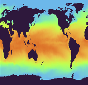
Finally, we turn to the problem of El Niño-Southern Oscillation (ENSO), i.e. cycles of warm (El Niño) and cold (La Niña) water temperature in the Pacific ocean near the equator. It is known that reconstructing ENSO features from sparse measurements is challenging (Manohar et al. Reference Manohar, Brunton, Kutz and Brunton2018; Maulik et al. Reference Maulik, Fukami, Ramachandra, Fukagata and Taira2020). Here, we focus on the El Niño event of the winter of 1997–1998, which is well known for its intensity off the coast of Peru. In particular, figure 8(a) shows the SST in December 1997. This snapshot lies in the test data set when the sets are chosen at random as opposed to sequentially. We see that the overall reconstruction error using vector-DEIM is larger compared with tensor-DEIM. More importantly, the spatial error near the El Niño oscillation is significantly larger when using vector-DEIM. Therefore, tensor-DEIM more successfully reconstructs the El Niño patterns. This is quite counter-intuitive since vector-DEIM tends to place more sensors in the El Niño region (see figure 5(c) off the coast of Peru).

Figure 8. Comparing the spatial distributions of the error. (a) True SST from December 1997. (b) Spatial distribution of error (reconstructed SST minus true SST) for vector-DEIM. (c) Spatial distribution of error for tensor-DEIM.
3.3. Three-dimensional unsteady flow
We consider a data set obtained by the simulation of an incompressible 3-D flow around a CAD model of the research vessel Tangaroa (Popinet, Smith & Stevens Reference Popinet, Smith and Stevens2004). This data set is obtained by large-eddy simulation using the Gerris flow solver (Popinet Reference Popinet2004). The flow variables are resampled onto a regular grid in the spatial region of interest,  $[-0.35, 0.65] \times [-0.3, 0.3] \times [-0.5, -0.3]$. The reported spatial variables are dimensionless, normalized with the characteristic length scale $L=276$ m, four times the ship length. Flow velocity is normalized by the inflow velocity $U=1$ m s $^{-1}$. We consider only the $u$ component of the velocity $(u,v,w)$ and subsampled the data to consider a grid size $150\times 90\times 60$. We split the available $201$ snapshots into a training data set with $150$ snapshots ( ${\sim }75\,\%$) and a test data set with $61$ snapshots.
Due to the enormous size of the resulting tensor, we used randomized SVD to compute the factor matrices  $\boldsymbol{\varPhi} _n$ for $1 \leq n \leq 3$ via the MATLAB command svdsketch. We choose $5\times 5 \times 5 = 125$ sensors to reconstruct the flow field. The true $u$-velocity for a snapshot in the test data set is plotted in figure 9(a). The reconstruction using tensor-DEIM is displayed in panel (b) of the same figure. The relative error in the reconstruction is around $9\,\%$ suggesting that tensor-DEIM is adequately reconstructing the snapshot. The corresponding error for the same number of sensors using vector-DEIM is $20.08\,\%$. As in the previous examples, it is seen that tensor-DEIM is far more accurate than vector-DEIM for the same number of sensors. The average relative error over the entire test data is $9.07\,\%$ for tensor-DEIM and $41.79\,\%$ for vector-DEIM. For some snapshots, the error in vector-DEIM is as high as $75\,\%$ and the error appears to increase for the later snapshots. Finally, the cost of storing the tensor-DEIM factor matrices is $0.0015\,\%$ of the cost of storing the vector-DEIM basis. Once again, tensor-DEIM proves to be more accurate and far more storage efficient compared with vector-DEIM.

Figure 9. (a) The true  $u$-velocity from the test data set. (b) Reconstruction using tensor-DEIM with $125$ sensors. Black dots indicate the position of the sensors; RE denotes the relative error.
4. Conclusions
Our results make a strong case for using tensor-based methods for sensor placement and flow reconstruction. In particular, our tensor-based method significantly increases the reconstruction accuracy and reduces its storage cost. Our numerical examples show that the relative reconstruction errors are comparable to vectorized methods when the number of sensors is small. However, as the number of sensors increases, our tensor-based method is 2–3 times more accurate than its vectorized counterpart. The improvements in terms of the storage cost are even more striking: tensor-DEIM requires only 0.0015 %–0.07 % of the memory required by vector-DEIM.
Future work could include the application of the method to reacting flows. In such flows, the multidimensional nature of our tensor-based method allows for separate optimal sensor placement for the flow field and each chemical species. Although our method is a tensorized version of DEIM, a similar tensor-based approach can be applied to other flow reconstruction methods such as gappy POD, sparsity-promoting methods, and autoencoders.
Acknowledgements
The authors would like to acknowledge the NOAA Optimum Interpolation (OI) SST V2 data provided by the NOAA PSL, Boulder, Colorado, USA, from their website at https://psl.noaa.gov. We would also like to thank the Computer Graphics Lab (ETH Zurich) for making the 3-D unsteady flow data used in § 3.3 publicly available. A.K.S. would also like to acknowledge I. Huang for her help with the figures.
Funding
This work was supported, in part, by the National Science Foundation through the awards DMS-1821149 and DMS-1745654, and Department of Energy through the award DE-SC0023188.
Declaration of interests
The authors report no conflict of interest.
Data availability statement
Appendix A. Proof of Theorem 1
We will need the following notation for the proof. We express  $\boldsymbol {\mathcal {Y}} = \boldsymbol {\mathcal {G}} \times _1 \boldsymbol {A}_1 \cdots \times \boldsymbol {A}_d$ in terms of unfoldings as $\boldsymbol {\mathcal {Y}}_{d} = \boldsymbol {A}_d \boldsymbol {Y}_{(d)} ( \boldsymbol {A}_{d-1} \otimes \cdots \otimes \boldsymbol {A}_1)^\top$. Here, we use $\otimes$ to denote the Kronecker product of two matrices.
The proof is similar to Kirsten (Reference Kirsten2022, Proposition 1). Using the properties of matrix unfoldings and Kronecker products, we can write an equivalent expression for the error:
 \begin{equation} \| \boldsymbol{\mathcal{G}} - \boldsymbol{\mathcal{G}} \times_{n=1}^d \boldsymbol{\varPi}_n\|_F = \| (\boldsymbol{I} - \otimes_{n=d}^1 \boldsymbol{\varPi}_n) \boldsymbol{G}_{(d+1)}^\top\|_F. \end{equation}
From  $\boldsymbol{\varPi} _n\boldsymbol{\varPhi} _n\boldsymbol{\varPhi} _n^\top =\boldsymbol{\varPhi} _n\boldsymbol{\varPhi} _n^\top$, we get $(\boldsymbol {I} - \otimes _{n=d}^1 \boldsymbol{\varPi} _n)(\boldsymbol{I} - \otimes _{n=d}^1 \boldsymbol{\varPhi} _n\boldsymbol{\varPhi} _n^\top ) = \boldsymbol{I} -\otimes _{n=d}^1 \boldsymbol{\varPi} _n$. Using this result and submultiplicativity,
 \begin{align} \| (\boldsymbol{I}- \otimes_{n=d}^1\boldsymbol{\varPi}_n)\boldsymbol{G}_{(d+1)}^\top\|_F &= \| (\boldsymbol{I} - \otimes_{n=d}^1 \boldsymbol{\varPi}_n)(\boldsymbol{I} - \otimes_{n=d}^1 \boldsymbol{\varPhi}_n\boldsymbol{\varPhi}_n^\top) \boldsymbol{G}_{(d+1)}^\top\|_F \nonumber\\ &\leq \| (\boldsymbol{I}- \otimes_{n=d}^1 \boldsymbol{\varPi}_n) \|_2\| (\boldsymbol{I} - \otimes_{n=d}^1\boldsymbol{\varPhi}_n\boldsymbol{\varPhi}_n^\top)\boldsymbol{G}_{(d+1)}^\top\|_F . \end{align}
Since  $\boldsymbol{\varPi} _n$ is an oblique projector, so are $\otimes _{j=1}^d \boldsymbol{\varPi} _n$ and $\boldsymbol{I} - \otimes _{j=1}^d \boldsymbol{\varPi} _n$. By Szyld (Reference Szyld2006, Theorem 2.1), which applies since $\otimes _{j=1}^d \boldsymbol{\varPi} _n$ is neither zero nor the identity, $\|\boldsymbol{I} - \otimes _{j=1}^d \boldsymbol{\varPi} _n\|_2 = \|\otimes _{j=1}^d \boldsymbol{\varPi} _n \|_2 = \prod _{n=1}^d \|\boldsymbol{\varPi} _n\|_2$. In the last step, we have used the fact that the largest singular value of a Kronecker product is the product of the largest singular values. Therefore,
 \begin{align} \| (\boldsymbol{I}- \otimes_{n=d}^1\boldsymbol{\varPi}_n)\boldsymbol{G}_{(d+1)}^\top\|_F &\leq \left( \prod_{n=1}^d \| \boldsymbol{\varPi}_n\|_2 \right) \|(\boldsymbol{I} - \otimes_{n=d}^1\boldsymbol{\varPhi}_n \boldsymbol{\varPhi}_n^\top)\boldsymbol{G}_{(d+1)}^\top\|_F \nonumber\\ &= \left( \prod_{n=1}^d \| (\boldsymbol{S}_n^\top\boldsymbol{\varPhi}_n)^{{-}1}\|_2 \right) \|\boldsymbol{\mathcal{G}} - \boldsymbol{\mathcal{G}} \times_{n=1}^d \boldsymbol{\varPhi}_n\boldsymbol{\varPhi}_n^\top\|_F, \end{align}
since  $\boldsymbol{\varPhi} _n$ and $\boldsymbol{S}_n$ have orthonormal columns, so $\|\boldsymbol{\varPi} _n\|_2 = \|(\boldsymbol{S}_n^\top \boldsymbol{\varPhi} _n)^{-1}\|_2$. The result follows from Vannieuwenhoven et al. (Reference Vannieuwenhoven, Vandebril and Meerbergen2012, Corollary 5.2).


 Open access