


1. Introduction
Close-contact melting is observed commonly in daily life when butter is melted in a hot pan. Almost instantly, a thin liquid layer is formed between the melting butter and the hot pan surface. Then heat is conducted through the thin layer and the melt is squeezed continuously to the sides by the butter's weight. This special type of melting is actually encountered in various industrial and engineering applications. For instance, it is essential for development of heated drilling devices that can bore into ice by close-contact melting (Shreve Reference Shreve1962; Schüller & Kowalski Reference Schüller and Kowalski2017; Park et al. Reference Park, Kang, Lee, Jeong, Park and Lee2021), as well as design of platforms designated for standing on melting ice sheets (Lea & Stegall Reference Lea and Stegall1973). Other examples include analysing lubrication characteristics of moving sliders (Wilson Reference Wilson1976), and even development of self-burying nuclear reactors that can melt their way into the Earth's core once overheated (Emerman & Turcotte Reference Emerman and Turcotte1983). Note that in a regular melting process, a thick liquid layer grows continuously between the hot surface and the melting solid. This liquid layer creates a thermal resistance that decreases the heat transfer rate over time. On the other hand, the liquid layer formed in a close-contact melting process typically remains thin ( $<1$ mm) (Ziskind & Kozak Reference Ziskind and Kozak2018). Thus the heat transfer rates are significantly higher in comparison with a regular melting process. In fact, it was demonstrated that by initiating close-contact melting in finned latent heat thermal energy storage units, the melting rate can be enhanced by 2.5 times, in comparison with a regular melting process (Kozak, Rozenfeld & Ziskind Reference Kozak, Rozenfeld and Ziskind2014).
The above-mentioned possible applications have driven fundamental research of close-contact melting phenomena for various basic configurations. The first simple configuration examined was melting in a spherical shell, which was initially studied experimentally and theoretically (Moore & Bayazitoglu Reference Moore and Bayazitoglu1982), and then improved modelling capabilities were developed (Bahrami & Wang Reference Bahrami and Wang1987). The similar problem of close-contact melting in horizontal cylindrical capsules was also explored experimentally (Sparrow & Geiger Reference Sparrow and Geiger1986) as well as analytically (Bareiss & Beer Reference Bareiss and Beer1984). Further extensions of this model for an elliptical capsule were developed later (Fomin, Wilchinsky & Saitoh Reference Fomin, Wilchinsky and Saitoh2000). The dynamics of close-contact melting in a heated annulus was explored both experimentally and theoretically (Betzel & Beer Reference Betzel and Beer1988). An extensive analysis for close-contact melting in a rectangular enclosure with different aspect ratios and phase change materials was also performed (Hirata, Makino & Kaneko Reference Hirata, Makino and Kaneko1991). The problem of hot cylindrical (Moallemi & Viskanta Reference Moallemi and Viskanta1986) and spherical (Emerman & Turcotte Reference Emerman and Turcotte1983) bodies that melt through an infinite solid medium was also addressed. Finally, different physical effects for close-contact melting of rectangular blocks on heated surfaces were studied, such as sliding (Groulx & Lacroix Reference Groulx and Lacroix2006) and unsteady melting (Myers, Mitchell & Muchatibaya Reference Myers, Mitchell and Muchatibaya2008). For such simple configurations, the melting rate and molten layer thickness can usually be predicted via analytical models based on thin-layer approximation and other simplifying assumptions (Bejan Reference Bejan1992, Reference Bejan1994). One fundamental configuration that was explored extensively is close-contact melting of a vertical cylinder on a horizontal isothermal surface. Early works dealt with experimental and theoretical analysis of a vertical cylinder pressed by an external force on a hot horizontal surface (Saito et al. Reference Saito, Utaka, Akiyoshi and Katayama1985a, Reference Saito, Utaka, Akiyoshi and Katayamab). The influence of material type, surface temperature, applied force and cylinder dimensions was determined. The same case without external forcing was later investigated experimentally and theoretically (Moallemi, Webb & Viskanta Reference Moallemi, Webb and Viskanta1986). It was shown that an analytical model can be derived for the melt fraction under simplifying assumptions. The influence of more complex effects, such as the inclusion of nanoparticles (Hu et al. Reference Hu, Zhu, Li, Tu and Fan2018) and non-Newtonian viscoplastic properties (Kozak et al. Reference Kozak, Zeng, Al Ghossein, Khodadadi and Ziskind2019), was also addressed recently. The similar case of an isothermal vertical cylindrical capsule has also been investigated (Saito et al. Reference Saito, Utaka, Shinoda and Katayama1986; Chen et al. Reference Chen, Cheng, Luo and Gu1993). Note that accurate prediction of the melting process in this case is much more involved due to interaction between natural convection in the melt and solid bulk motion. A full solution of this problem has been achieved only recently (Shockner & Ziskind Reference Shockner and Ziskind2021), as it requires specially designed numerical methods (see, for instance, Gudibande & Iyer Reference Gudibande and Iyer2017; Kasibhatla et al. Reference Kasibhatla, König-Haagen, Rösler and Brüggemann2017; Kozak & Ziskind Reference Kozak and Ziskind2017; Faden et al. Reference Faden, König-Haagen, Höhlein and Brüggemann2018; Pan et al. Reference Pan, Charles, Vermaak, Romero, Neti, Zheng, Chen and Bonner III2018; Kasibhatla & Brüggemann Reference Kasibhatla and Brüggemann2021.
It has been demonstrated in the past that the hot surface structure can influence significantly the close-contact melting process. Saito, Hong & Hirokane (Reference Saito, Hong and Hirokane1992) proved, both experimentally and theoretically, that the heat transfer rate can be enhanced by slitting radial grooves in the surface. This configuration reduces the pressure in the molten layer leading to a thinner layer that creates a lower thermal resistance and higher heat transfer rates. Turkyilmazoglu (Reference Turkyilmazoglu2019) also demonstrated that the close-contact melting dynamics can be altered by using a permeable surface. Today, it is possible to design and fabricate micro-textured surfaces with remarkable properties (Ybert et al. Reference Ybert, Barentin, Cottin-Bizonne, Joseph and Bocquet2007). In particular, the surface roughness allows the liquid contact angle to exceed  $150^{\circ }$, yielding a non-wetting superhydrophobic surface (Chen, Guo & Liu Reference Chen, Guo and Liu2017). Two superhydrophobic states can be achieved: the Wenzel and Cassie states (Lafuma & Quéré Reference Lafuma and Quéré2003). For the Wenzel case, the liquid is impregnated inside the surface texture. On the other hand, for the Cassie case, gas pockets remain trapped in the surface texture, and a stable liquid–gas interface is established on the surface. Transition between Cassie and Wenzel states is also possible (Zheng, Yu & Zhao Reference Zheng, Yu and Zhao2005; Patankar Reference Patankar2010; Papadopoulos et al. Reference Papadopoulos, Mammen, Deng, Vollmer and Butt2013). For instance, the liquid–gas interface can collapse under high pressure conditions and wet the surface texture, leading to a Cassie–Wenzel transition (Xue et al. Reference Xue, Chu, Lv and Duan2012, Reference Xue, Lv, Lin and Duan2016; Emami et al. Reference Emami, Hemeda, Amrei, Luzar, Gad-el Hak and Vahedi Tafreshi2013; Hemeda & Tafreshi Vahedi Reference Hemeda and Tafreshi Vahedi2014; Lv et al. Reference Lv, Xue, Shi, Lin and Duan2014; Fang et al. Reference Fang, Guo, Li, Li and Feng2018).
In recent years, superhydrophobic surfaces in the Cassie state have shown great promise for various applications, such as drag reduction (Lauga & Stone Reference Lauga and Stone2003; Ou, Perot & Rothstein Reference Ou, Perot and Rothstein2004; Liravi et al. Reference Liravi, Pakzad, Moosavi and Nouri-Borujerdi2020), enhanced condensation heat transfer (Miljkovic, Enright & Wang Reference Miljkovic, Enright and Wang2013), anti-icing (Hejazi, Sobolev & Nosonovsky Reference Hejazi, Sobolev and Nosonovsky2013) and thermal insulation (Shao, Wang & Bai Reference Shao, Wang and Bai2020). However, the phenomenon of close-contact melting on superhydrophobic surfaces has not been investigated either experimentally or theoretically. It is known that superhydrophobic surfaces in the Cassie state induce partial hydrodynamic slip, due to the trapped gas pockets (Rothstein Reference Rothstein2010). Drag is reduced as gases are typically less viscous than liquids (Lee, Choi & Kim Reference Lee, Choi and Kim2016). Potentially, superhydrophobic surfaces can reduce the pressure in the thin molten layer, which is governed by viscous forces (Ockendon & Ockendon Reference Ockendon and Ockendon1995). As a result, the molten layer thickness can decrease and the heat transfer rate can be enhanced, similarly to the approach suggested by Saito et al. (Reference Saito, Hong and Hirokane1992). Nevertheless, superhydrophobic surfaces also induce thermal slip, due to imperfect thermal contact between the solid surface and the liquid layer (Enright et al. Reference Enright, Hodes, Salamon and Muzychka2014; Steigerwalt Lam et al. Reference Steigerwalt Lam, Melnick, Hodes, Ziskind and Enright2014). This effect can impede the heat transfer rates. A recent study by Aljaghtham, Premnath & Alsulami (Reference Aljaghtham, Premnath and Alsulami2021) addressed this interplay between hydrodynamic and thermal slips for close-contact melting of a rectangular block under the influence of a magnetic field. The slip effects were modelled via Navier boundary conditions with arbitrary chosen slip lengths. It was found that the effect of hydrodynamic slip alone increases the melting rate, whereas the inclusion of thermal slip decreases the melting rate. Nevertheless, the dynamics of this interplay for close-contact melting on a superhydrophobic surface with a certain micro-texture, temperature and melting material is unclear. Also, the conditions for a stable liquid–gas interface that retains the Cassie state under a close-contact melting process are unknown currently.
In the current work, we present, for the first time, a detailed derivation of a numerical model for close-contact melting of a vertical cylinder on a horizontal isothermal superhydrophobic surface with an array of circular posts. Predictions of the melt fraction, molten layer thickness and heat transfer rate, for a representative case of an ice cylinder, are shown. An approximate analytical model is derived as well, and its range of validity is investigated. Finally, a conservative criterion for the liquid–gas interface stability under close-contact melting conditions is established.
2. Theoretical model formulation
The general schematics of the numerical model that will be developed in this section are shown in figure 1. Figure 1(a) presents an isometric view of a superhydrophobic surface with an equidistant array of circular posts, where  $h$ denotes the post height. The top view of this surface is presented in figure 1(b), where $d$ is the post diameter, and $l$ is the distance between two posts. Figure 1(c) presents the physical problem, close-contact melting of an ice cylinder on an isothermal superhydrophobic surface. The cylinder has initial radius and height $R$ and $H$, respectively, whereas the upper surface position is denoted by $s$. Also, the $r$ and $z$ coordinate system used for the model formulation is shown. A thin molten layer with thickness $\delta$ is formed between the ice and the hot surface. Due to gravity $g$, the melt in the layer is squeezed to the sides by the ice cylinder's own weight. Figure 1(d) shows representative examples of the resulting velocity and temperature profiles, $u$ and $T$, in the thin molten layer. The surface and ice melting temperatures, $T_w$ and $T_m$, respectively, are presented, as well as the hydrodynamic and thermal slip lengths, $\lambda$ and $\lambda _t$, respectively.
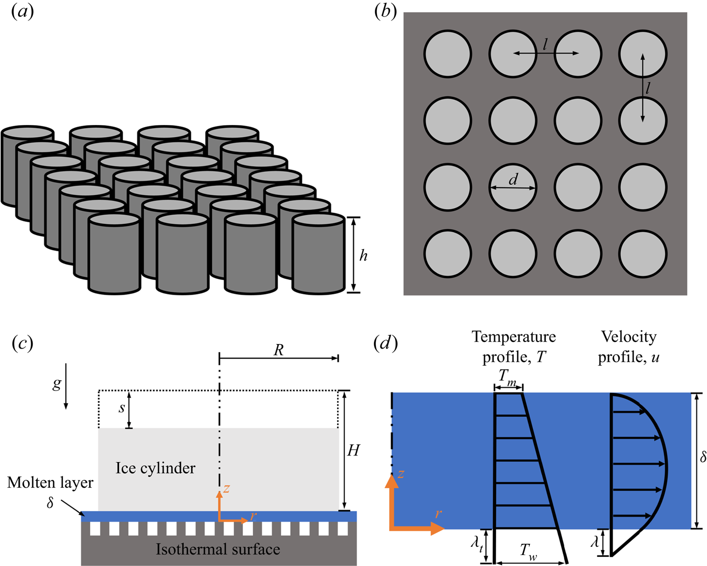
Figure 1. General schematics of the numerical model. (a) Isometric view of a superhydrophobic surface with an equidistant array of circular posts. (b) Top view of the surface. (c) Close-contact melting of an ice cylinder on an isothermal superhydrophobic surface. (d) The flow and heat transfer in the thin molten layer.
The model is based on the following assumptions: (a) thin-layer approximation, hence the molten layer thickness is much smaller than the cylinder's dimensions; (b) the upper ice interface shape remains flat; (c) sensible heating effects are negligible; (d) the flow in the thin molten layer is laminar; (e) the ice motion as well as the flow and heat transfer in the thin molten layer are quasi-steady; (f) the effect of convection in the melt is negligible; (g) material properties are constant; (h) pressure gradients in the  $z$-direction are negligible; (i) the solid surface is perfectly isothermal; (j) heat transfer through the gas layers is negligible; (k) the substrate pattern effect can be modelled via an effective slip length. Note that assumptions (a)–(h) are typical for close-contact melting problems and were validated experimentally for different configurations (Bareiss & Beer Reference Bareiss and Beer1984; Moallemi & Viskanta Reference Moallemi and Viskanta1986; Bejan Reference Bejan1994). Although some of these assumptions can be relaxed (see, for instance, Yoo, Hong & Kim Reference Yoo, Hong and Kim1998; Groulx & Lacroix Reference Groulx and Lacroix2003, Reference Groulx and Lacroix2007; Cregan, Williams & Myers Reference Cregan, Williams and Myers2020), the contribution of these additional physical effects on the melting rate is usually not significant for low Stefan and high Prandtl numbers. Assumptions (i) and (j) are valid only for sufficiently high ratios between the solid surface and gas thermal conductivities. Assumption (k) indicates that the alternating slip/no-slip boundary condition induced by the substrate pattern can be modelled via boundary condition homogenization. As the description of wetting hydrodynamics requires a microscopic model to avoid contact line singularity, the Navier slip boundary condition with an appropriate slip length is utilized; see Snoeijer & Andreotti (Reference Snoeijer and Andreotti2013) for a detailed discussion.
The range of validity of assumptions (i) and (j) can be estimated by the analysis presented below. The thermal resistances of the solid and gas layers,  $R_s$ and $R_g$, respectively, are
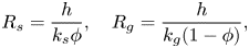 \begin{equation} R_s=\frac{h}{k_s{\phi}},\quad R_g=\frac{h}{k_g(1-\phi)}, \end{equation}
where  $h$ is the post height, $k_s$ and $k_g$ are the solid surface and gas thermal conductivities, respectively, and $\phi$ is the solid surface volume fraction, which is given by the following analytical expression for the considered geometry:
 \begin{equation} \phi=\frac{{\rm \pi}d^2}{4l^2}. \end{equation}
Assumption (i) is valid as long as the thermal resistance of the solid layer is sufficiently small. A criterion for estimating this assumption validity can be formulated as
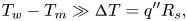 \begin{equation} T_w-T_m\gg {\rm \Delta}{T}=q''R_s, \end{equation}
where  $q''$ is the heat flux, and ${\rm \Delta} {T}$ is the temperature difference across the solid layer, i.e. the temperature difference between the base and the top of each post. Equation (2.3) states that the temperature difference between the surface and the melting point is much greater than the temperature difference across the solid surface. Thus the temperature difference across the solid surface can be considered negligible. Equation (2.1a,b) can be substituted into (2.3) yielding the condition
 \begin{equation} k_s\gg \frac{q''{h}}{(T_w-T_m)\phi}, \end{equation}
 For typical values  $q''=10^5$ W m $^{-2}$, $h=10\,\mathrm {\mu }$m, $T_w-T_m=10$ K and $\phi =0.01$, (2.4) yields $k_s\gg 10$ W mK $^{-1}$, which is applicable for several possible solid surface materials.
Assumption (j) is valid as long as the gas layer thermal resistance is significantly higher than the solid layer thermal resistance:
 \begin{equation} R_g\gg R_s. \end{equation}
Substitution of (2.1a,b) into (2.5) yields
 \begin{equation} \frac{k_s}{k_g}\gg \frac{1-\phi}{\phi}. \end{equation}
 For a relatively low value of  $\phi =0.01$, (2.6) provides approximately the condition $k_s/k_g\gg 100$. This condition holds for many solid and gas material combinations. However, it is clear that the analysis above indicates that assumptions (i) and (j) are not valid in general.
It is important to stress that  $\phi$ is also connected to the wall wettability, according to Quéré (Reference Quéré2008):
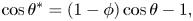 \begin{equation} \cos\theta^{*}=(1-\phi)\cos\theta-1, \end{equation}
where  $\theta$ and $\theta ^*$ are the contact angle and the apparent contact angle, respectively. Thus for low values of $\phi$, the surface wettability decreases as the apparent contact angle increases. Also, although the micro-structure pattern has no cylindrical symmetry, according to assumption (k), a homogeneous Navier slip boundary can be applied for the macro-scale cylindrical symmetric flow. This assumption is valid as the substrate micro-structure pattern is smaller by several orders of magnitude in comparison with the macro-scale flow.
Following assumptions (a)–(k), a numerical model for close-contact melting on isothermal superhydrophobic surfaces can be formulated. The model will be able to predict the resulting melting rate, molten layer thickness and heat transfer rate for given conditions. First, the momentum equation for the  $r$-direction velocity component under thin-layer approximation (see assumption (a)) is invoked:
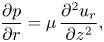 \begin{equation} \frac{\partial p}{\partial r}=\mu\,\frac{\partial^2 u_r}{\partial z^2}, \end{equation}
where  $p$ is pressure, $\mu$ is dynamic viscosity, and $u_r$ is the $r$-direction velocity component. Equation (2.8) can be integrated twice with respect to $z$ to derive an expression for the radial velocity profile:
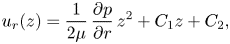 \begin{equation} u_r(z)=\frac{1}{2\mu}\,\frac{\partial p}{\partial r}\,z^2+C_1z+C_2, \end{equation}
where  $C_1$ and $C_2$ are integration constants. Two boundary conditions are applied for finding the integration constants values: the Navier boundary condition (Rothstein Reference Rothstein2010) for partial slip at the superhydrophobic surface (
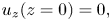
 $z=0$), and the no-slip condition at the solid ice surface ( $z=\delta$):
 $$\begin{gather} u_r(z=0)=\lambda\,\frac{\partial u_r}{\partial z}(z=0), \end{gather}$$
 $$\begin{gather}u_r(z=\delta)=0, \end{gather}$$
where  $\lambda$ is the hydrodynamic slip length (Davis & Lauga Reference Davis and Lauga2010). The integration constants $C_1$ and $C_2$ can be determined by substituting (2.9) into (2.10) and (2.11):
 $$\begin{gather} C_1={-}\frac{1}{2\mu(\lambda+\delta)}\,\frac{\partial p}{\partial r}\,\delta^2, \end{gather}$$
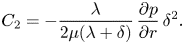 $$\begin{gather}C_2={-}\frac{\lambda}{2\mu(\lambda+\delta)}\,\frac{\partial p}{\partial r}\,\delta^2. \end{gather}$$
 The following expression for the  $r$-direction velocity profile in the thin molten layer can be found by substituting (2.12) and (2.13) back into (2.9):
 \begin{equation} u_r(z)=\frac{1}{2\mu}\,\frac{\partial p}{\partial r} \left(z^2-\frac{\delta^2}{\lambda+\delta}\,[z+\lambda]\right). \end{equation}
The two-dimensional radial continuity equation is invoked for finding the pressure distribution in the thin molten layer:
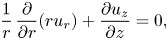 \begin{equation} \frac{1}{r}\,\frac{\partial}{\partial r}(ru_r)+\frac{\partial u_z}{\partial z}=0, \end{equation}
where  $u_z$ is the $z$-direction velocity component. Equation (2.15) can be integrated with respect to $z$ across the thin molten layer:
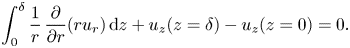 \begin{equation} \int_{0}^{\delta}\frac{1}{r}\,\frac{\partial}{\partial r}(ru_r)\,{\rm d} z+u_z(z=\delta)-u_z(z=0)=0. \end{equation}
 Two boundary conditions can be applied: a no-penetration condition at the superhydrophobic surface ( $z=0$), and the solid velocity at the ice surface ( $z=\delta$):
 $$\begin{gather} u_z(z=0)=0, \end{gather}$$
 $$\begin{gather}u_z(z=\delta)={-}\frac{{\rm d} s}{{\rm d} t}, \end{gather}$$
where  $s$ is the upper solid surface position and $t$ is time. By substituting (2.14), (2.17) and (2.18) into (2.16), the following expression can be derived:
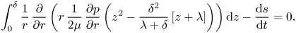 \begin{equation} \int_{0}^{\delta}\frac{1}{r}\,\frac{\partial}{\partial r} \left(r\,\frac{1}{2\mu}\,\frac{\partial p}{\partial r} \left(z^2-\frac{\delta^2}{\lambda+\delta}\,[z+\lambda]\right)\right){\rm d} z-\frac{{\rm d} s}{{\rm d} t}=0. \end{equation}
Integration of (2.19) yields the following differential equation for the pressure distribution:
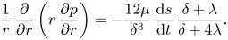 \begin{equation} \frac{1}{r}\,\frac{\partial}{\partial r}\left(r\,\frac{\partial p}{\partial r}\right)={-}\frac{12\mu}{\delta^3}\, \frac{{\rm d} s}{{\rm d} t}\,\frac{\delta+\lambda}{\delta+4\lambda}. \end{equation}
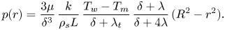
 An explicit expression for the pressure can be derived by integrating (2.20) twice with respect to  $r$:
$r$:
 \begin{equation} p(r)={-}\frac{3\mu}{\delta^3}\,\frac{{\rm d} s}{{\rm d} t}\, \frac{\delta+\lambda}{\delta+4\lambda}\,r^2+C_3\ln(r)+C_4, \end{equation}
where  $C_3$ and $C_4$ are integration constants. The integration constants can be found via two boundary conditions: zero pressure gradient at the cylinder's centre ( $r=0$), and zero gauge pressure at the thin molten layer outlet ( $r=R$):
 $$\begin{gather} \frac{\partial p}{\partial r}(r=0)=0, \end{gather}$$
 $$\begin{gather}p(r=R)=0. \end{gather}$$
 The integration constants  $C_3$ and $C_4$ are determined by substituting (2.21) into (2.22) and (2.23):
 $$\begin{gather} C_3=0, \end{gather}$$
 $$\begin{gather}C_4=\frac{3\mu}{\delta^3}\,\frac{{\rm d} s}{{\rm d} t}\,\frac{\delta+\lambda}{\delta+4\lambda}\,R^2. \end{gather}$$
The pressure distribution in the thin molten layer can be derived by substituting (2.24) and (2.25) back into (2.21):
 \begin{equation} p(r)=\frac{3\mu}{\delta^3}\,\frac{{\rm d} s}{{\rm d} t}\,\frac{\delta+\lambda}{\delta+4\lambda}\,(R^2-r^2). \end{equation}
The heat transfer equation in the thin molten layer, under assumptions (e) and (f), is invoked for finding the solid velocity:
 \begin{equation} \frac{\partial^2 T}{\partial z^2}=0, \end{equation}
where  $T$ is temperature. Equation (2.27) can be integrated twice with respect to $z$, yielding the expression
 \begin{equation} T(z)=C_5z+C_6, \end{equation}
where  $C_5$ and $C_6$ are integration constants. The integration constants are determined via two boundary conditions: thermal slip (Steigerwalt Lam et al. Reference Steigerwalt Lam, Melnick, Hodes, Ziskind and Enright2014) at the superhydrophobic surface ( $z=0$), and melting point temperature at the ice surface ( $z=\delta$):
 $$\begin{gather} T_w-T(z=0)={-}\lambda_t\,\frac{\partial T}{\partial z}(z=0), \end{gather}$$
 $$\begin{gather}T(z=\delta)=T_m, \end{gather}$$
where  $T_w$ and $T_m$ are the wall and melting point temperatures, respectively, and $\lambda _t$ is the thermal slip length (Enright et al. Reference Enright, Hodes, Salamon and Muzychka2014). By substituting (2.28) into (2.29) and (2.30), the integration constants $C_5$ and $C_6$ can be determined:
 $$\begin{gather} C_5=\frac{T_m-T_w}{\delta+\lambda_t}, \end{gather}$$
 $$\begin{gather}C_6=T_w+\lambda_t\,\frac{T_m-T_w}{\delta+\lambda_t}. \end{gather}$$
The temperature distribution in the thin molten layer can be found by substituting (2.31) and (2.32) back into (2.28):
 \begin{equation} T(z)=T_w+\frac{T_m-T_w}{\delta+\lambda_t}\,(z+\lambda_t). \end{equation}
The Stefan condition (Alexiades & Solomon Reference Alexiades and Solomon2018), under assumption (c), can be utilized for coupling the heating rate and the solid interface velocity:
 \begin{equation} \rho_s{L}\,\frac{{\rm d} s}{{\rm d} t}={-}k\,\frac{{\rm d} T}{{\rm d} z}(z=\delta), \end{equation}
where  $\rho _s$ is the solid phase density, $L$ is latent heat of fusion per unit mass, and $k$ is the liquid phase thermal conductivity. The solid velocity can be found by substituting (2.33) into (2.34):
 \begin{equation} \frac{{\rm d} s}{{\rm d} t}=\frac{k}{\rho_s{L}}\,\frac{T_w-T_m}{\delta+\lambda_t}. \end{equation}
An explicit relation between the pressure distribution and the molten layer thickness can now be derived by substituting (2.35) into (2.26):
 \begin{equation} p(r)=\frac{3\mu}{\delta^3}\,\frac{k}{\rho_s{L}}\,\frac{T_w-T_m}{\delta+\lambda_t}\, \frac{\delta+\lambda}{\delta+4\lambda}\,(R^2-r^2). \end{equation}
The force balance between the pressure forces and the solid weight, under assumption (e), is invoked for finding a relation between the molten layer thickness and the solid upper interface position:
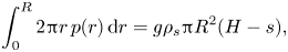 \begin{equation} \int_{0}^{R}2{\rm \pi}{r\,p(r)}\,{\rm d} r=g\rho_s{\rm \pi}{R^2}(H-s), \end{equation}
where  $H$ is the ice cylinder's initial height, and $g$ is the gravitational acceleration. Equation (2.36) can be substituted into (2.37), and after integration, the following relation can be derived:
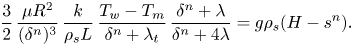
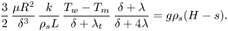 \begin{equation} \frac{3}{2}\,\frac{\mu{R^2}}{\delta^3}\,\frac{k}{\rho_s{L}}\, \frac{T_w-T_m}{\delta+\lambda_t}\,\frac{\delta+\lambda}{\delta+4\lambda}=g\rho_s(H-s). \end{equation}
Equations (2.35) and (2.38) comprise a set of first-order ordinary differential and nonlinear algebraic equations, respectively, that can be solved numerically for the solid melting rate and molten layer thickness. For the model closure, a relation for the hydrodynamic and thermal slip lengths should be provided. For the hydrodynamic slip length, we will utilize a simple theoretical expression from Davis & Lauga (Reference Davis and Lauga2010) for a superhydrophobic surface with circular posts, which is applicable for  $\phi<0.2$:
 \begin{equation} \frac{\lambda}{l}=\frac{3}{16}\sqrt{\frac{\rm \pi}{\phi}}-\frac{3}{2{\rm \pi}}\ln(1+\sqrt{2}), \end{equation}
where  $l$ is the distance between two posts, and $\phi$ is the solid volume fraction of the surface material. The thermal slip length can be derived by the following expression from Enright et al. (Reference Enright, Hodes, Salamon and Muzychka2014) that relates the hydrodynamic and thermal slip lengths:
 \begin{equation} \lambda=\tfrac{3}{4}\lambda_t. \end{equation}
Substituting (2.39) into (2.40) yields the following expression for the thermal slip length:
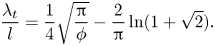 \begin{equation} \frac{\lambda_t}{l}=\frac{1}{4}\sqrt{\frac{\rm \pi}{\phi}}-\frac{2}{\rm \pi}\ln(1+\sqrt{2}). \end{equation}
Note that the distance between two posts,  $l$, depends on the post diameter $d$ and the solid volume fraction $\phi$ via the relation (Hemeda & Tafreshi Vahedi Reference Hemeda and Tafreshi Vahedi2014)
 \begin{equation} l=\sqrt{\frac{{\rm \pi}{d^2}}{4\phi}}. \end{equation}
3. Limiting case – perfect slip and thermal contact
It is of interest to investigate a limiting case that offers an analytical solution for (2.35) and (2.38). In particular, the case of perfect hydrodynamic slip and thermal contact (constant surface temperature) will reveal the maximum possible theoretical enhancement in the melting rate by a superhydrophobic surface. It is clear that existing superhydrophobic surfaces always induce both hydrodynamic and thermal slip. Nevertheless, it is of interest to understand the role of reduced thermal slip, as in the future, different techniques for reducing thermal slip, while still maintaining high hydrodynamic slip, can be introduced. Therefore, the maximum possible enhancement in the melting time by superhydrophobic surfaces can be used to determine the practical usefulness of thermal slip reduction. This case corresponds to the limits  $\lambda \rightarrow \infty$ and $\lambda _t\rightarrow 0$. It is also equivalent for replacing (2.10) and (2.29) with perfect slip and constant surface temperature conditions, respectively. Under this limiting case, (2.38) is simplified to the form
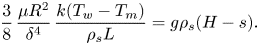 \begin{equation} \frac{3}{8}\,\frac{\mu{R^2}}{\delta^4}\,\frac{k(T_w-T_m)}{\rho_s{L}}=g\rho_s(H-s). \end{equation}
The molten layer thickness  $\delta$ can now be isolated:
 \begin{equation} \delta = \left[\frac{3}{8}\,\frac{\mu{R^2}}{g\rho_s(H-s)}\,\frac{k(T_w-T_m)}{\rho_s{L}}\right]^{1/4}. \end{equation}
 Equation (3.2) can be substituted into (2.35) under the limit  $\lambda _t\rightarrow 0$ to yield the ordinary differential equation
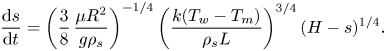 \begin{equation} \frac{{\rm d} s}{{\rm d} t}=\left(\frac{3}{8}\,\frac{\mu{R^2}}{g\rho_s}\right)^{{-}1/4} \left(\frac{k(T_w-T_m)}{\rho_s{L}}\right)^{3/4}(H-s)^{1/4}. \end{equation}
Equation (3.3) can be solved analytically via variable separation and integration:
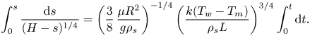 \begin{equation} \int_{0}^{s}\frac{{\rm d} s}{(H-s)^{1/4}}=\left(\frac{3}{8}\, \frac{\mu{R^2}}{g\rho_s}\right)^{{-}1/4}\left(\frac{k(T_w-T_m)}{\rho_s{L}}\right)^{3/4}\int_{0}^{t}{\rm d} t. \end{equation}
Integration of (3.4) yields an analytical solution for the solid upper interface position as a function of time:
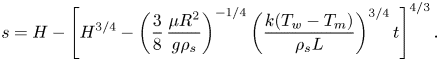 \begin{equation} s=H-\left[H^{3/4}-\left(\frac{3}{8}\,\frac{\mu{R^2}}{g\rho_s}\right)^{{-}1/4} \left(\frac{k(T_w-T_m)}{\rho_s{L}}\right)^{3/4}t\right]^{4/3}. \end{equation}
The total melting time is the time when the solid upper interface reaches the surface, and it can be found by substituting  $s=H$ into (3.5):
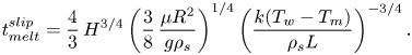 \begin{equation} t_{{melt}}^{{slip}}=\frac{4}{3}\,H^{3/4}\left(\frac{3}{8}\,\frac{\mu{R^2}}{g\rho_s}\right)^{1/4} \left(\frac{k(T_w-T_m)}{\rho_s{L}}\right)^{{-}3/4}. \end{equation}
Note that the classical analytical solution with a no-slip boundary condition at the hot isothermal surface by Moallemi et al. (Reference Moallemi, Webb and Viskanta1986) predicts the following melting time, under the same conditions:
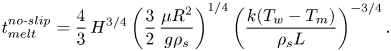 \begin{equation} t_{{melt}}^{{no\text{-}slip}}=\frac{4}{3}\,H^{3/4}\left(\frac{3}{2}\,\frac{\mu{R^2}}{g\rho_s}\right)^{1/4} \left(\frac{k(T_w-T_m)}{\rho_s{L}}\right)^{{-}3/4}. \end{equation}
The ratio between (3.6) and (3.7) provides an analytical relation for the maximum possible enhancement in the melting time by using a superhydrophobic surface:
 \begin{equation} t_{{melt}}^{{slip}}/t_{{melt}}^{{no\text{-}slip}}=1/\sqrt{2}\approx70\,\%, \end{equation}
Equation (3.8) reveals that for perfect hydrodynamic slip and thermal contact, it is possible theoretically to decrease the melting time by about  $30\,\%$ in comparison with a regular isothermal surface with a no-slip boundary condition.
4. Numerical model solution method
The model governing equations (2.35) and (2.38) do not admit an analytical solution and must be solved numerically. Equation (2.35) can be discretized by a simple forward Euler scheme:
 \begin{equation} s^{n+1}=s^n+\frac{k}{\rho_s{L}}\,\frac{T_w-T_m}{\delta^n+\lambda_t}\,{\rm \Delta}{t}, \end{equation}
where  $n$ and $n+1$ denote the current and next time steps, respectively, and ${\rm \Delta} {t}$ is discrete time step. The nonlinear algebraic equation (2.38) can be solved in a coupled manner with (4.1) via the scheme
 \begin{equation} \frac{3}{2}\,\frac{\mu{R^2}}{(\delta^n)^3}\,\frac{k}{\rho_s{L}}\, \frac{T_w-T_m}{\delta^n+\lambda_t}\,\frac{\delta^n+\lambda}{\delta^n+4\lambda}=g\rho_s(H-s^n). \end{equation}
Also, the following initial condition, which states that the initial upper solid interface position is zero, is applied:
 \begin{equation} s(t=0)=0. \end{equation}
For each time step, (4.2) is solved for  $\delta ^n$ via a nonlinear algebraic equation solver. Then the new interface position, $s^{n+1}$, is calculated via (4.1). Note that the hydrodynamic and thermal slip lengths, $\lambda$ and $\lambda _t$, are calculated via (2.39) and (2.41), respectively. For the first time step,
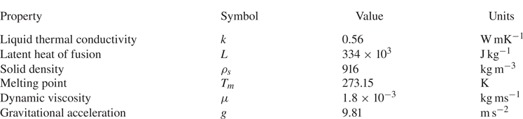
  $s^n=0$ according to (4.3). The material properties of ice and water that are utilized in the current study, as well as relevant parameter values, can be found in table 1. Also, a time step ${\rm \Delta} {t}=10^{-3}$ s was found to be sufficiently small for proper convergence of all the tested cases.
Table 1. Material properties and parameter values.
5. Numerical model results and discussion
The predictions of the numerical model, which was formulated in § 2, are presented and discussed in the current section. The model is explored for a representative case with wall temperature  $T_w=293.15$ K, cylinder height and radius $H=R=1$ cm, and post diameter $d=6\,\mathrm {\mu }$m, whereas the distance between two posts, $l$, can be determined according to (2.42). The chosen values correspond to realistic close-contact melting on regular surfaces experiments (Saito et al. Reference Saito, Utaka, Akiyoshi and Katayama1985a; Moallemi et al. Reference Moallemi, Webb and Viskanta1986) and superhydrophobic surface geometry from the literature (Lobaton & Salamon Reference Lobaton and Salamon2007), which was utilized for other applications. Note that the micro-structure substrate pattern was found to impact significantly the surface wettability and slip length (Ou et al. Reference Ou, Perot and Rothstein2004). This is in accordance with different theoretical predictions; see Lobaton & Salamon (Reference Lobaton and Salamon2007) and Davis & Lauga (Reference Davis and Lauga2010). The effect of the surface solid volume fraction $\phi$, for values 0.16, 0.08, 0.04, 0.02 and 0.01, is explored. The results are compared against the classical analytical solution for a regular isothermal surface with a no-slip boundary condition by Moallemi et al. (Reference Moallemi, Webb and Viskanta1986):
 \begin{equation} s_{{no\text{-}slip}}=H-\left[H^{3/4}-\left(\frac{3}{2}\,\frac{\mu{R^2}}{g\rho_s}\right)^{{-}1/4} \left(\frac{k(T_w-T_m)}{\rho_s{L}}\right)^{3/4}t\right]^{4/3}. \end{equation}
 First, the melt fraction, which equals  $s/H$, as a function of time is presented in figure 2. The results demonstrate that for relatively high $\phi$ values, the melting progression is only slightly slower than the no-slip perfect thermal contact case. However, for lower values of $\phi$, the melting time increases much more significantly, whereas for the lowest value, $\phi =0.01$, the total melting time is roughly doubled. The results reveal that the thermal slip has a much more dominant effect than the hydrodynamic slip on the melting rate as the melting time increases monotonically with the decrease of $\phi$.
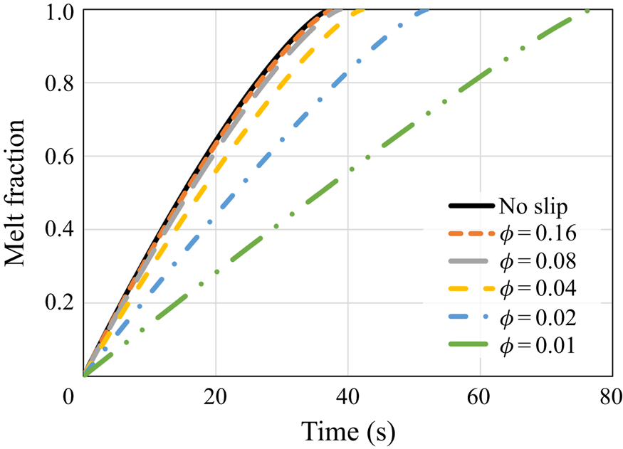
Figure 2. The melt fraction as a function of time according to the predictions of the numerical model and the classical no-slip constant wall temperature analytical solution (5.1). Different values of the surface solid volume fraction  $\phi$ are examined.
The dynamics of the melting process is explored further in figure 3, which presents the molten layer thickness,  $\delta$, as a function of time, for all the same cases. The analytical solution for the molten layer thickness under no-slip and constant surface temperature conditions is
 \begin{equation} \delta_{{no\text{-}slip}}=\left(\frac{3}{2}\,\frac{k(T_w-T_m)\mu{R^2}}{g\rho_s^2{L}(H-s_{{no\text{-}slip}})}\right)^{1/4}. \end{equation}
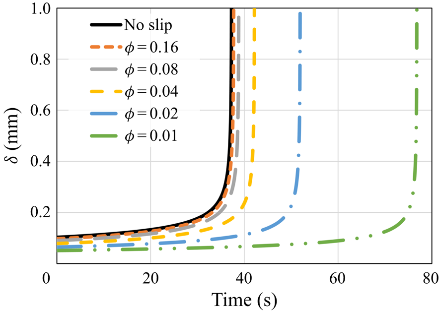
Figure 3. The molten layer thickness  $\delta$ as a function of time according to the predictions of the numerical model and the classical no-slip constant wall temperature analytical solution (5.2). Different values of the surface solid volume fraction $\phi$ are examined.
In a manner similar to the results presented in figure 2, for relatively high values of  $\phi$, the molten layer thickness is only slightly decreased in comparison with the classical no-slip analytical solution. Also, for lower values of $\phi$, the molten layer thickness is reduced significantly in a monotonic trend due to the hydrodynamic slip. Although this reduction should decrease the molten layer thermal resistance and thus increase the melting rate, the thermal slip creates an additional, much higher, thermal resistance that increases the melting time. It is stressed that the rapid increase in the molten layer thickness at the end of the melting process is due to the very low remaining solid mass. It is clear that once the molten layer thickness is sufficiently large, the assumption of a thin molten layer does not hold. Nevertheless, this situation occurs only after most of the solid material has melted and thus does not affect significantly the overall melting process.
In addition, these resulting trends are investigated by calculating the heat flux at the surface via the right-hand side of the Stefan condition (see (2.34)):
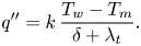 \begin{equation} q''=k\,\frac{T_w-T_m}{\delta+\lambda_t}. \end{equation}
The heat flux for a no-slip constant temperature surface can be derived by the analytical expression
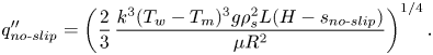 \begin{equation} q''_{{no\text{-}slip}}=\left(\frac{2}{3}\,\frac{k^3(T_w-T_m)^3g\rho_s^2{L}(H-s_{{no\text{-}slip}})}{\mu{R^2}}\right)^{1/4}. \end{equation}
 Figure 4 shows the numerical model and the analytical solution results for the heat flux. In general, the heat flux decreases monotonically as  $\phi$ decreases. Yet a very slight decrease in the heat flux in comparison with the no-slip analytical solution is observed for relatively high values of $\phi$. For lower values of $\phi$, the decrease in the heat flux is much more substantial. For $\phi =0.01$, the reduction at $t=0$ s is more than two times in comparison with a regular no-slip surface. According to (5.3), it is clear that as $k$,
$k$,  $T_w$ and $T_m$ are constants, and the molten layer thickness $\delta$ is lower than the no-slip case (see figure 3), the lower heat flux must be a result of high values of thermal slip length $\lambda _t$.
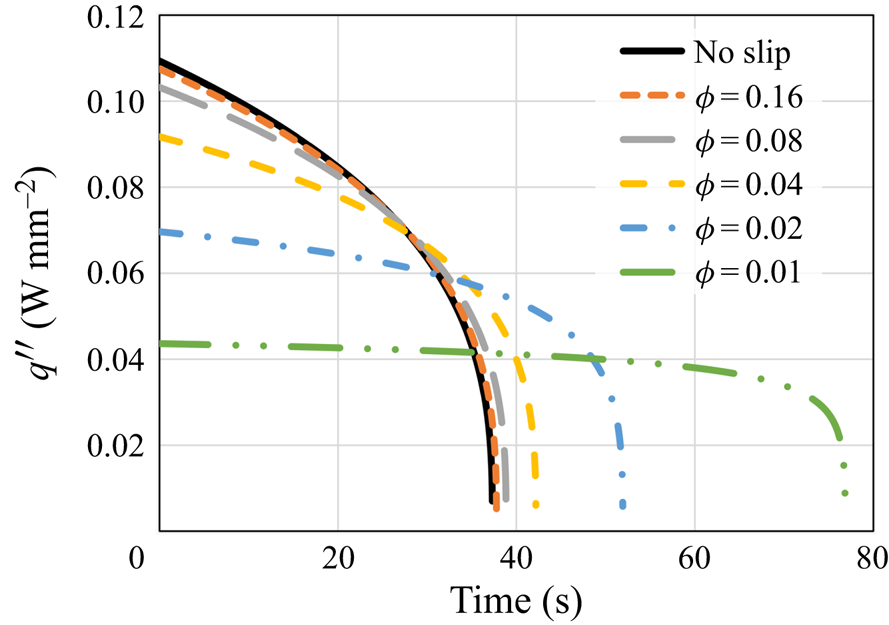
Figure 4. The heat flux  $q''$ as a function of time according to the predictions of the numerical model and the classical no-slip constant surface temperature analytical solution (5.4). Different values of the surface solid volume fraction $\phi$ are examined.
6. Approximate analytical model
The numerical model developed in the previous sections provides an accurate solution of the problem governing equations. However, it is of interest to develop an approximate analytical model that will reveal some of the basic features of the problem and provide quick estimations. Two approximate assumptions can be applied to achieve this goal: (1)  $\lambda \approx \lambda _t$; (2) $4\lambda \gg \delta$. It is worth noting that assumption (1) leads to a constant error of 33 % in the hydrodynamic slip length (see (2.40)), and assumption (2) can never hold at the final stages of the melting as $\delta \rightarrow \infty$ (see figure 3). Nevertheless, it will be demonstrated that under certain conditions, the predictions of an analytical approximate model, which is governed by assumptions (1) and (2), can provide excellent agreement with the numerical model results.
Under assumptions (1) and (2), (2.38) can be reduced into the form
 \begin{equation} \frac{3}{8}\,\frac{\mu{R^2}}{\delta^3}\,\frac{k}{\rho_s{L}}\,\frac{T_w-T_m}{\lambda_t}=g\rho_s(H-s). \end{equation}
 Equation (6.1) allows us to isolate the molten layer thickness  $\delta$:
 \begin{equation} \delta=\left(\frac{3}{8}\,\frac{\mu{R^2}}{g\rho_s^2(H-s)}\,\frac{k}{L}\,\frac{T_w-T_m}{\lambda_t}\right)^{1/3}. \end{equation}
 Also, an explicit expression for the heat flux  $q''$ can be obtained by substituting (6.2) into (5.3):
 \begin{equation} q''=k\,\frac{T_w-T_m}{\left(\dfrac{3}{8}\,\dfrac{\mu{R^2}}{g\rho_s^2(H-s)}\, \dfrac{k}{L}\,\dfrac{T_w-T_m}{\lambda_t}\right)^{1/3}+\lambda_t}. \end{equation}
 Both (6.2) and (6.3) depend on the time-dependent upper solid interface position  $s$. An explicit relation between $s$ and time can be found by substituting (6.2) into (2.35) and applying integration:
 \begin{equation} \int_{0}^{s}\left[\left(\frac{3}{8}\,\frac{\mu{R^2}}{g\rho_s^2(H-s)}\,\frac{k}{L}\, \frac{T_w-T_m}{\lambda_t}\right)^{1/3}+\lambda_t\right]{\rm d} s=k\,\frac{T_w-T_m}{\rho_s{L}}\int_{0}^{t}{\rm d} t. \end{equation}
 The resulting solution of (6.4) provides the following analytical relation between the upper interface position  $s$ and time $t$:
$t$:
 \begin{equation} \frac{3}{2}\,\left(\frac{3}{8}\,\frac{\mu{R^2}}{g\rho_s^2}\, \frac{k}{L}\,\frac{T_w-T_m}{\lambda_t}\right)^{1/3} \left(H^{2/3}-(H-s)^{2/3}\right)+\lambda_t{s}=k\,\frac{T_w-T_m}{\rho_s{L}}\,t. \end{equation}
 The predictions derived by the analytical approximate model are compared against the numerical model results to determine the analytical model applicability and general trends. Figures 5(a–e) present the melt fraction as a function of time, for both the analytical and numerical models, for the same  $\phi$ values and conditions as presented in § 4. In general, the analytical model overpredicts the total melting time, and the discrepancy between the analytical and numerical model is significant for relatively high values of $\phi$; see figures 5(a,b). However, the analytical model provides better predictions as the value of $\phi$ decreases (see figure 5c), and for low $\phi$ values, the agreement between the analytical and numerical models is excellent (see figures 5d,e). It is worth noting that the trends of the melting time with the decrease of $\phi$ are very different between the two models. For the numerical model, the melting time increases monotonically as $\phi$ decreases. Yet for the analytical model, the trend is non-monotonic. As $\phi$ decreases, the melting time decreases; see figures 5(a,b,c). Then as $\phi$ decreases further, the melting time increases; see figures 5(d,e). These non-monotonic trends are attributed to assumption (2). For high $\phi$ values, the slip length is small, thus $\delta$ cannot be considered negligible in comparison with $4\lambda$. As a result, the slip length continues to affect the solution even for very low slip length values. Thus the solution does not converge to the classical no-slip solution for low slip length values, which leads to a non-physical trend for the melting time.
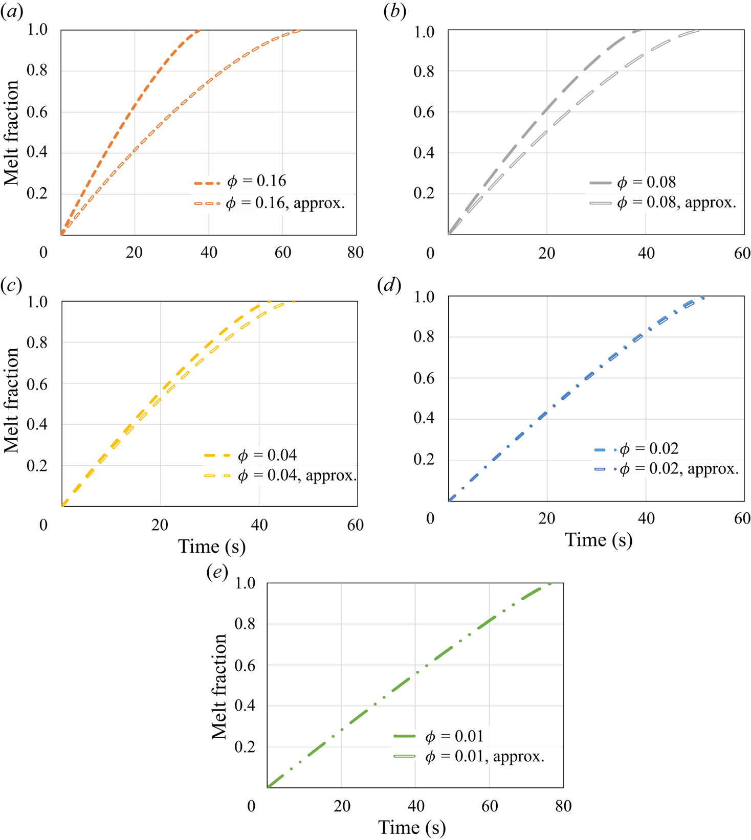
Figure 5. The melt fraction as a function of time – comparison between the numerical and approximate analytical models for: (a)  $\phi =0.16$, (b) $\phi =0.08$, (c) $\phi =0.04$, (d) $\phi =0.02$, (e) $\phi =0.01$.
The predictions of the molten layer thickness  $\delta$ as a function of time are also compared between the analytical and numerical models under the same conditions; see figures 6(a–e). The analytical model overpredicts the molten layer thickness, and the discrepancy between the two models is significant for $\phi =0.16$ and $\phi =0.08$; see figures 6(a,b). However, as the value of $\phi$ decreases, the predictions improve (see figure 6c) and provide excellent estimation for low $\phi$ values (see figures 6d,e). Opposed to the melt fraction predictions, both the numerical and analytical models show the same trends – the molten layer thickness decreases as $\phi$ decreases.
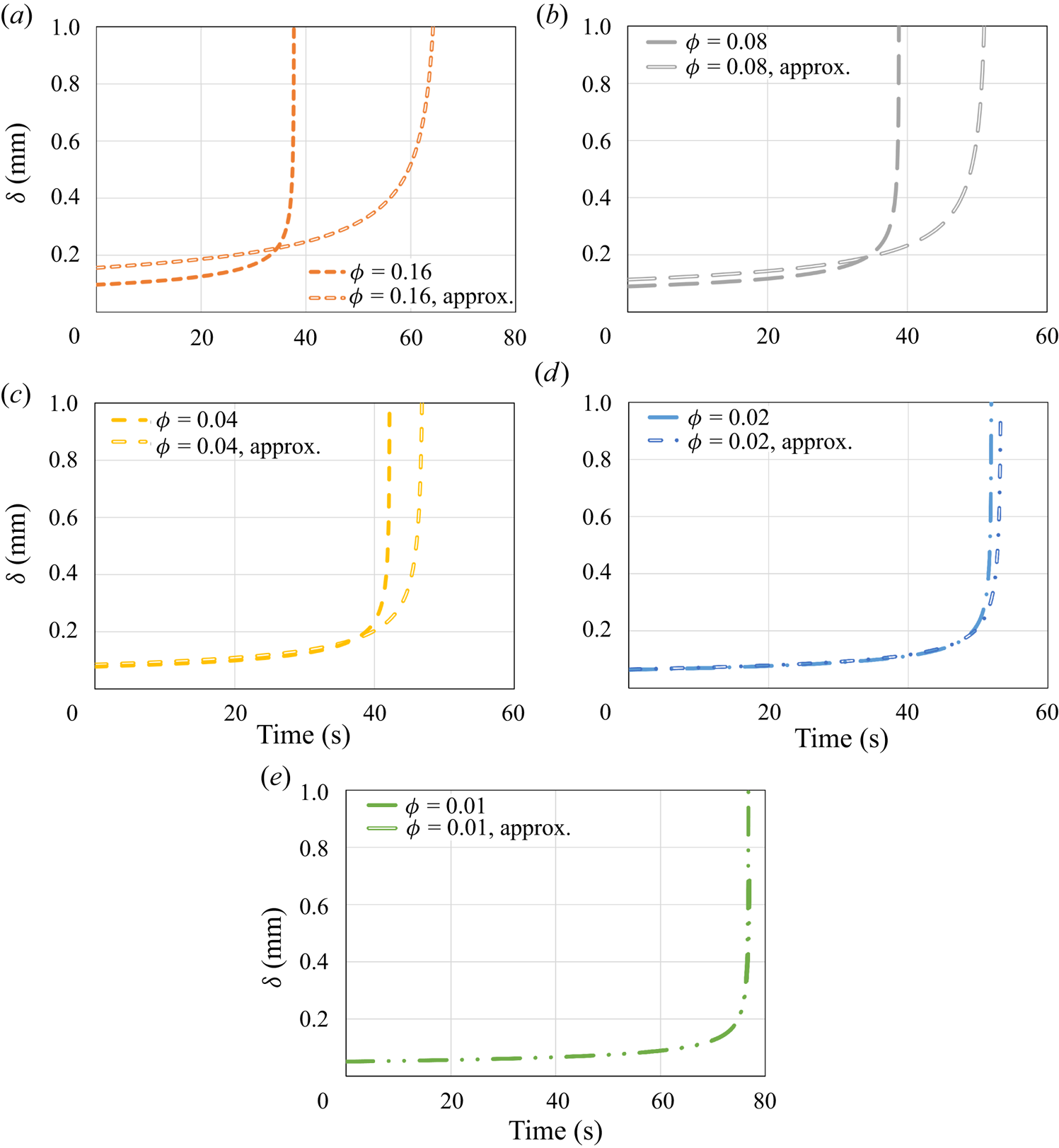
Figure 6. The molten layer thickness  $\delta$ as a function of time – comparison between the numerical and approximate analytical models for: (a) $\phi =0.16$, (b) $\phi =0.08$, (c) $\phi =0.04$, (d) $\phi =0.02$, (e) $\phi =0.01$.
Further comparison between the two models involves the predicted heat flux; see figures 7(a–e). The heat flux is underpredicted by the analytical model, and the agreement improves as  $\phi$ decreases; see figures 7(a,b,c). For sufficiently low $\phi$ values, the two models provide almost indistinguishable results; see figures 7(d,e). The trends predicted by the two models differ. For the numerical model, the heat flux is decreasing monotonically with the decrease in $\phi$, whereas for the analytical model, as $\phi$ decreases, the heat flux increases (see figures 7a,b,c) and then decreases (see figures 7d,e).
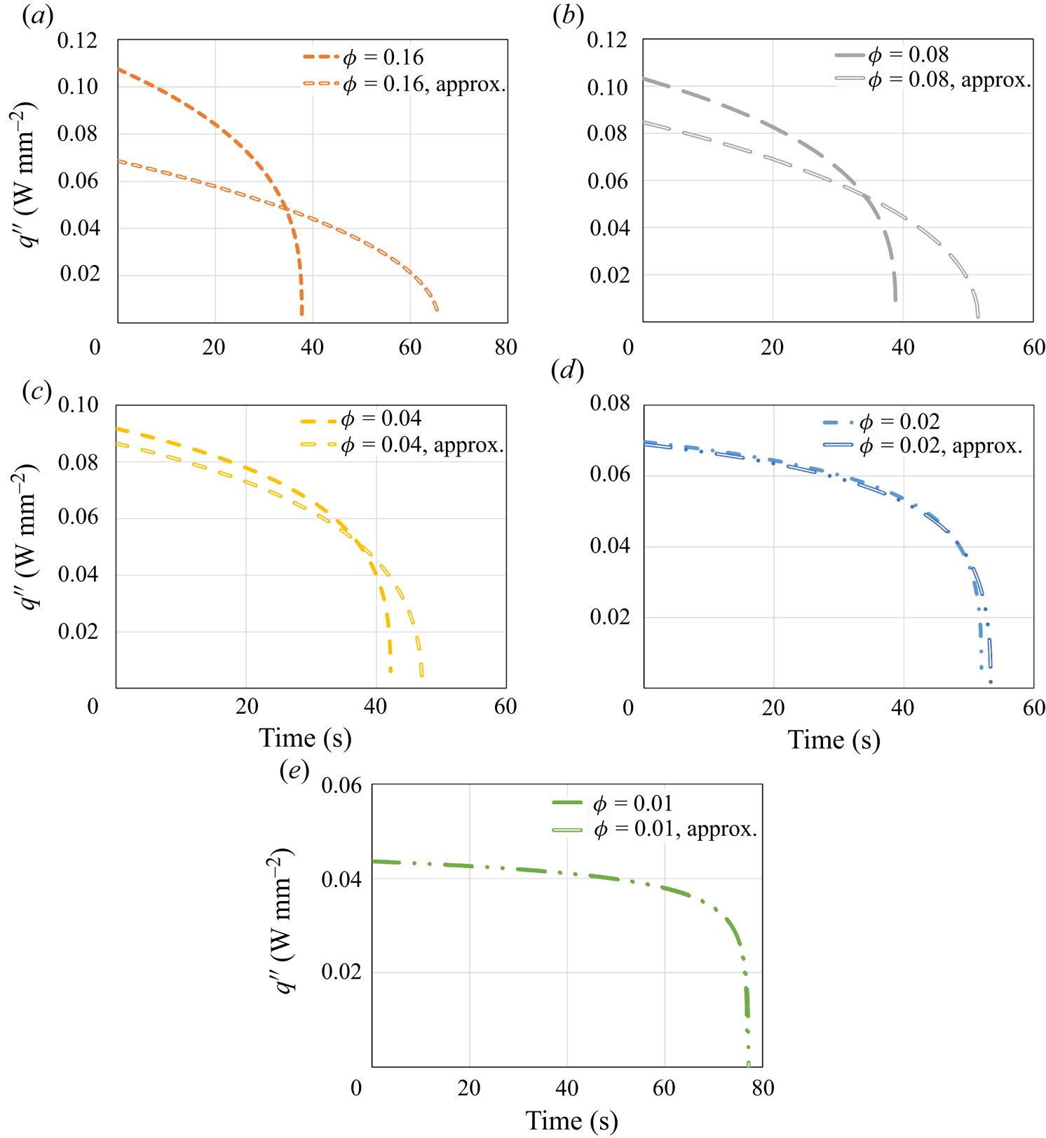
Figure 7. The heat flux  $q''$ as a function of time – comparison between the numerical and approximate analytical models for: (a) $\phi =0.16$, (b) $\phi =0.08$, (c) $\phi =0.04$, (d) $\phi =0.02$, (e) $\phi =0.01$.
The approximate analytical model can also provide a formula for the total melting time,  $t_{{melt}}$, by substituting $s=H$ into (6.5):
 \begin{equation} t_{{melt}}=\frac{3}{2}\,H^{2/3}\left(\frac{3}{8}\,\frac{\mu{R^2}}{g\rho_s\lambda_t}\right)^{1/3} \left(k\,\frac{T_w-T_m}{L\rho_s}\right)^{{-}2/3}+\lambda_t{H}\left(k\,\frac{T_w-T_m}{L\rho_s}\right)^{{-}1}. \end{equation}
The analytical relation presented in (6.6) can be used for deriving an expression for the ratio of the melting times between isothermal superhydrophobic and regular surfaces (see also (3.7)):
 \begin{equation} \frac{t_{{melt}}}{t_{{melt}}^{{no\text{-}slip}}}=\left(\frac{3}{2}\right)^{{-}1/4} \frac{3}{4}\left[\frac{3}{4}\,3^{1/3}\left(\frac{\mu{R^2}}{gH\lambda_t^4}\,k\, \frac{T_w-T_m}{L\rho_s^2}\right)^{1/12}+\left(\frac{\mu{R^2}}{gH\lambda_t^4}\,k\, \frac{T_w-T_m}{L\rho_s^2}\right)^{{-}1/4}\right]. \end{equation}
 Equation (6.7) reveals that the melting times ratio depends on a single dimensionless group that is denoted here as  $\varepsilon$, where
 \begin{equation} \varepsilon=\frac{\mu{R^2}}{gH\lambda_t^4}\,k\,\frac{T_w-T_m}{L\rho_s^2}. \end{equation}
 Substitution of (6.8) into (6.7) yields the following expression, which is a function of only  $\varepsilon$:
 \begin{equation} \frac{t_{{melt}}}{t_{{melt}}^{{no\text{-}slip}}}=f(\varepsilon)=\left(\frac{3}{2}\right)^{{-}1/4}\frac{3}{4} \left[\frac{3}{4}\,3^{1/3}\varepsilon^{1/12}+\varepsilon^{{-}1/4}\right]. \end{equation}
 Equation (6.9) can be differentiated with respect to  $\varepsilon$ and equated to zero to find an extremum point:
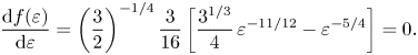 \begin{equation} \frac{{\rm d} f(\varepsilon)}{{\rm d}\varepsilon}=\left(\frac{3}{2}\right)^{{-}1/4} \frac{3}{16}\left[\frac{3^{1/3}}{4}\,\varepsilon^{{-}11/12}-\varepsilon^{{-}5/4}\right]=0. \end{equation}
 Solution of (6.10) yields  $\varepsilon _{{ext}}$, the $\varepsilon$ value at the extremum point:
 \begin{equation} \varepsilon_{{ext}}=\frac{64}{3}. \end{equation}
 Equation (6.10) can be differentiated again with respect to  $\varepsilon$ to find whether the extremum point is a maximum or minimum:
 \begin{equation} \frac{{\rm d}^2f(\varepsilon)}{{\rm d}\varepsilon^2}=\left(\frac{3}{2}\right)^{{-}1/4} \frac{3}{64}\left[-\frac{11}{12}\,3^{1/3}\varepsilon^{{-}23/12}+5\varepsilon^{{-}9/4}\right]. \end{equation}
Substitution of (6.11) into (6.12) yields a positive value, thus the point is minimum. Substitution of (6.11) into (6.9) finds the minimum ratio between the melting times of superhydrophobic and regular surfaces:
 \begin{equation} \left(\frac{t_{{melt}}}{t_{{melt}}^{{no\text{-}slip}}}\right)_{{min}}\approx{1.26}. \end{equation}
The analysis shows that the analytical model predicts that the melting time for a superhydrophobic surface will be greater by at least 26 % than a regular surface with no-slip and constant temperature boundary conditions. These results agree qualitatively with the numerical model predictions that showed that the melting time for superhydrophobic surfaces tends to increase. In order to investigate further the analytical model fundamental features, dimensional analysis is applied. The following dimensionless groups govern the problem:
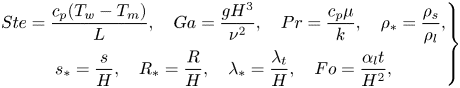 \begin{equation} \left.\begin{gathered} Ste=\frac{c_p(T_w-T_m)}{L},\quad Ga=\frac{gH^3}{\nu^2},\quad Pr=\frac{c_p{\mu}}{k},\quad \rho_*=\frac{\rho_s}{\rho_l}, \\ s_*=\frac{s}{H},\quad R_*=\frac{R}{H},\quad \lambda_*=\frac{\lambda_t}{H},\quad Fo=\frac{\alpha_l{t}}{H^2}, \end{gathered}\right\} \end{equation}
where  $Ste$ is the Stefan number, $Ga$ is the Galilei number, $Pr$ is the Prandtl number, $\rho _*$ is the solid–liquid density ratio, $s_*$ is the melt fraction, $R_*$ is dimensionless radius, $\lambda _*$ is dimensionless slip length, $Fo$ is the Fourier number, $c_p$ is specific heat, $\nu$ is kinematic viscosity, $\rho _l$ is the liquid phase density, and $\alpha _l$ is the liquid phase thermal diffusivity. Based on this analysis, (6.8) can be rendered into dimensionless form:
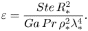 \begin{equation} \varepsilon=\frac{Ste\,R_*^2}{Ga\,Pr\,\rho_*^2\lambda_*^4}. \end{equation}
Equations (6.2) and (6.3) can also be rendered into dimensionless form:
 $$\begin{gather} \frac{\delta}{H}=\delta_*=\lambda_*\left(\frac{3}{8}\,\frac{\varepsilon}{1-s_*}\right)^{1/3}, \end{gather}$$
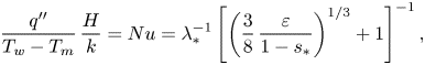 $$\begin{gather}\frac{q''}{T_w-T_m}\,\frac{H}{k}=Nu=\lambda_*^{{-}1}\left[\left(\frac{3}{8}\, \frac{\varepsilon}{1-s_*}\right)^{1/3}+1\right]^{{-}1}, \end{gather}$$
where  $\delta _*$ is the dimensionless molten layer thickness, and $Nu$ is the Nusselt number. The analytical solution reveals that both $\delta _*$ and $Nu$ depend on the dimensionless groups $\varepsilon$, $s_*$ and $\lambda _*$. Equation (6.5) can also be rendered into dimensionless form:
 \begin{equation} \frac{Ste\,Fo}{\lambda_*\rho_*}=\frac{3}{2} \left(\frac{3}{8}\,\varepsilon\right)^{1/3}(1-(1-s_*)^{2/3})+s_*. \end{equation}
 Although an explicit expression for  $s_*$ cannot be derived, it is clear that $s_*$ depends on two dimensionless groups: ${Ste\,Fo}/{\rho _*\lambda _*}$ and $\varepsilon$. An expression for the dimensionless melting time, $Ste\,Fo_{{melt}}$, can be yielded by substituting $s_*=1$ into (6.18):
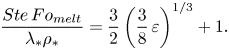 \begin{equation} \frac{Ste\,Fo_{{melt}}}{\lambda_*\rho_*}=\frac{3}{2}\left(\frac{3}{8}\,\varepsilon\right)^{1/3}+1. \end{equation}
Finally, the dimensionless analysis results will be used to determine a criterion for the analytical model range of applicability. Both assumptions (1) and (2) of the analytical model can be rendered into dimensionless form to yield the condition
 \begin{equation} 4\lambda_*\gg \delta_*. \end{equation}
Equation (6.16) can be substituted into (6.20) to yield the condition
 \begin{equation} 4\lambda_*\gg \lambda_*\left(\frac{3}{8}\,\frac{\varepsilon}{1-s_*}\right)^{1/3}, \end{equation}
The condition derived in (6.21) can be simplified into the form
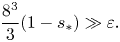 \begin{equation} \frac{8^3}{3}(1-s_*)\gg \varepsilon. \end{equation}
 It is clear that the condition stated in (6.22) can never hold in general, as for  $s_*=1$, it is always violated. However, for practical purposes, it is possible to assume that the analytical solution should provide sufficiently accurate results if 95 % of the melting process is captured correctly. Thus $s_*=0.95$ is substituted into (6.22), formalizing the following condition:
 \begin{equation} 8.5\gg \varepsilon. \end{equation}
 The condition in (6.23) indicates that for  $\varepsilon$ values sufficiently lower than 8.5, the approximate analytical model will replicate accurately the numerical model results. This result agrees with the analysis presented above as the cases $\phi =0.16$, 0.08, 0.04, 0.02 and 0.01 correspond to $\varepsilon$ values 26, 290, 574, 20, 0.8 and 0.04, respectively. Indeed, only the cases $\phi =0.02$ and 0.01, where the criterion of (6.23) was satisfied, proved to capture accurately the numerical model results. This analysis is summarized in figure 8, where the melting time ratio as a function of $\varepsilon$, (6.9), is presented as well as the minimum point, (6.13), and the approximate model applicability condition, (6.23). It is stressed that the minimum point (see (6.13)) does not satisfy the approximate model validity criterion (see (6.23)). Thus (6.13) captures the melting time increase trend only qualitatively but not quantitatively. Note that the non-monotonic trends observed above by the analytical model are associated with high $\varepsilon$ values that lead to inaccurate and non-physical predictions of the numerical model results.
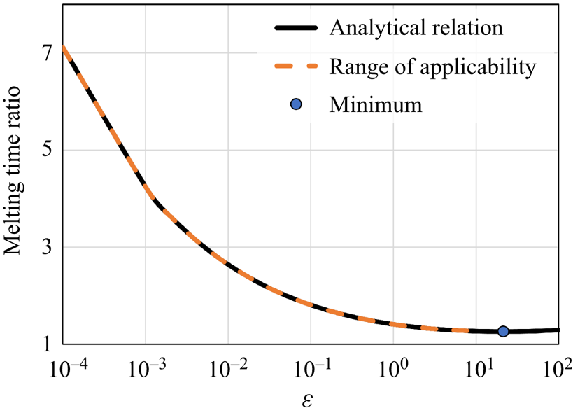
Figure 8. The melting time ratio between close-contact melting on superhydrophobic and regular surfaces as a function of  $\varepsilon$, based on the approximate analytical model predictions: the analytical relation (6.9), the analytical model range of applicability (6.23), and the minimum point (6.13).
7. Stability of the liquid–gas interface
The previous sections dealt with the dynamics of close-contact melting on superhydrophobic surfaces. However, it is assumed implicitly that the liquid–gas interface remains stable, thus the Cassie state is maintained throughout the entire melting process. This is not an obvious assumption, as it is known that for sufficiently high pressure, the liquid–gas interface can collapse and transition into a Wenzel state (Fang et al. Reference Fang, Guo, Li, Li and Feng2018). Many studies analysed the conditions for this transition to occur (Lobaton & Salamon Reference Lobaton and Salamon2007; Xue et al. Reference Xue, Chu, Lv and Duan2012, Reference Xue, Lv, Lin and Duan2016), as well as the liquid–gas interface longevity under unstable conditions (Emami et al. Reference Emami, Hemeda, Amrei, Luzar, Gad-el Hak and Vahedi Tafreshi2013; Hemeda & Tafreshi Vahedi Reference Hemeda and Tafreshi Vahedi2014). The situation in the current problem is even more complex than other cases dealt with in the literature as the pressure in the thin molten layer depends on both space and time. Moreover, it is possible that the finite time that the liquid–gas interface takes to collapse is much larger than the melting time. Although it is possible to formulate a rather complicated and exact model that will take into account these effects, in the current work a much simpler approach is devised. It is possible to formulate a conservative condition that guarantees the liquid–gas interface stability under the assumption of worst scenario conditions. Accordingly, the maximum pressure, for both space and time, occurs at the cylinder's centre  $r=0$, at the beginning of the melting process $t=0$. The maximum pressure $p_{{max}}$ at the cylinder's centre can be derived by substituting $r=0$ into (2.36):
 \begin{equation} p_{{max}}=p(r=0)=\frac{3\mu{R^2}}{\delta^3}\,\frac{k}{\rho_s{L}}\, \frac{T_w-T_m}{\delta+\lambda_t}\,\frac{\delta+\lambda}{\delta+4\lambda}. \end{equation}
 Equation (7.1) can be substituted into (2.38) under the constraint  $s(t=0)=0$, to derive a very simple relation for the maximum possible pressure for both space and time:
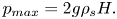 \begin{equation} p_{{max}}=2g\rho_s{H}. \end{equation}
 It is therefore assumed that the pressure is constant and equal to  $p_{{max}}$. The liquid–gas interface becomes unstable once the external pressure equals the capillary pressure (Lobaton & Salamon Reference Lobaton and Salamon2007). Thus the condition for the liquid–gas interface stability is
 \begin{equation} 2g\rho_s{H}={-}\frac{4\sigma\cos{\theta}}{D_{{cap}}^{{eq}}}, \end{equation}
where  $D_{{cap}}^{{eq}}$ is the equivalent pore diameter – defined by Hemeda & Tafreshi Vahedi (Reference Hemeda and Tafreshi Vahedi2014) for simplifying the interface stability analysis – $\sigma$ is surface tension, and $\theta$ is the advancing contact angle. According to (7.3), a critical cylinder height can be defined that renders the liquid–gas interface unstable:
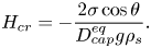 \begin{equation} H_{cr}={-}\frac{2\sigma\cos{\theta}}{D_{{cap}}^{{eq}}g\rho_s}. \end{equation}
For a superhydrophobic surface with an array of equidistant circular posts, the equivalent pore diameter can be defined as (see Hemeda & Tafreshi Vahedi Reference Hemeda and Tafreshi Vahedi2014)
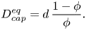 \begin{equation} D_{{cap}}^{{eq}}=d\,\frac{1-\phi}{\phi}. \end{equation}
Equation (7.5) can be substituted into (7.4) to derive the following condition for the critical cylinder height:
 \begin{equation} H_{cr}={-}\frac{2\sigma\cos{\theta}}{g\rho_s{d}}\,\frac{\phi}{1-\phi}. \end{equation}
 Note that (7.6) provides a conservative estimate. Thus cylinder height values lower than  $H_{cr}$ must lead to a stable state. However, for higher height values, a more precise analysis is needed to determine whether or not the conditions lead to a stable state. The critical height predicted by (7.6) is presented in figure 9 as a function of $\phi$. The surface conditions are chosen based on realistic superhydrophobic surfaces from the literature (see Lobaton & Salamon (Reference Lobaton and Salamon2007)), using the same post diameter and material properties as in the analysis above. The value of $\sigma$ is 72.8 mN m $^{-1}$. Two values of $\theta$ are examined, based on the measurements in Lobaton & Salamon (Reference Lobaton and Salamon2007). Clearly, as the advancing contact angle increases, the liquid–gas interface stability is improved. It can be seen that for $\theta =122.1^{\circ }$, a cylinder's height of 1 cm, as used in the current study, should not lead to a collapse of the liquid–gas interface even for surface volume fractions $\phi$ as low as 0.01.
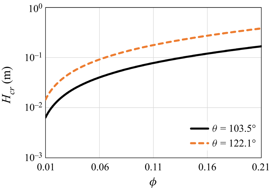
Figure 9. The critical cylinder's height for the liquid–gas interface stability as a function of the surface volume fraction  $\phi$; see (7.6). Two different advancing contact angles $\theta$ are examined.
8. Conclusion
In the present study, the problem of close-contact melting of a vertical cylinder on a horizontal isothermal superhydrophobic surface has been analysed theoretically. A new numerical model has been derived, under several simplifying assumptions. The model can predict the melt fraction, molten layer thickness and heat transfer rate for a superhydrophobic surface with an array of equidistant circular posts. It is demonstrated that under the limit of perfect slip and constant surface temperature, an analytical solution for the melting time can derived. This solution reveals that for any close-contact melting process of a vertical cylinder on a horizontal isothermal superhydrophobic surface, the possible melting time enhancement, in comparison with a regular no-slip surface, cannot exceed 30 %. Numerical solution of the model governing equations, for a representative case of an ice cylinder, shows that for relatively high surface volume fractions,  $\phi >0.04$, the effect of the superhydrophobic surface on the melting rate, molten layer thickness and heat transfer rate is negligible. However, for lower $\phi$ values, the close-contact melting process on a superhydrophobic surface can be roughly two times longer than the case for a regular surface. The analysis shows that although the thin molten layer thickness is decreased, the overall heat transfer rate is decreased due to the thermal slip effect, which proves dominant.
An approximate analytical model is developed for gaining fundamental understanding of the problem dynamics and fast estimations. The new analytical model predictions are compared extensively against the numerical model results. For low  $\phi$ values, the analytical model provides excellent agreement with the numerical model results. For high $\phi$ values, the analytical model overpredicts the melting time and the molten layer thickness, and underpredicts the heat transfer rate. Also, the analytical model can reproduce the correct physical trend for the molten layer thickness as $\phi$ is varied. On the other hand, the trends, as $\phi$ is varied, for the melt fraction and heat transfer rate do not agree with the numerical model results. Dimensional analysis reveals that according to the analytical model predictions, the ratio between the melting times for superhydrophobic and regular surfaces is governed by a single dimensionless group, $\varepsilon =Ste\,R_*^2/Ga\,Pr\,\rho _*^2\lambda _*^4$. It is also proved that according to the analytical model predictions, the melting time on a superhydrophobic surface is always longer by more than 26 % in comparison with a regular surface. This result agrees qualitatively with the numerical model predictions that show that the melting time on a superhydrophobic surface is always longer than on a regular surface. Based on this analysis, it is shown that for $\varepsilon \ll 8.5$, the analytical model provides an excellent estimate of the numerical model results. Finally, a conservative criterion for the liquid–gas interface stability is derived. It is demonstrated that the Cassie state can be maintained throughout the entire close-contact melting process for all the cases studied in the current work. It is stressed that the current model provides, for the first time, quantitative predictions for the phenomenon of close-contact melting on superhydrophobic surfaces. Thus in the future, the model limitations should be assessed carefully against high-fidelity simulations and experimental results. Moreover, the role of metastability will be explored in detail; see, for instance, (Poole et al. Reference Poole, Sciortino, Essmann and Stanley1992; Palmer et al. Reference Palmer, Martelli, Liu, Car, Panagiotopoulos and Debenedetti2014; Magaletti, Gallo & Casciola Reference Magaletti, Gallo and Casciola2021). Future work will deal with the close-contact melting dynamics of additional surface micro-textures and simple geometric configurations. Also, the liquid–gas interface longevity under close-contact melting conditions will be studied in detail.
Acknowledgements
The author would like to thank Prof G. Ziskind of Ben-Gurion University of the Negev for introducing him to the field of solid–liquid phase change and many helpful discussions throughout the years.
Funding
This research received no specific grant from any funding agency, or commercial or not-for-profit sectors.
Declaration of interests
The author reports no conflict of interest.


 Open access