


1. Introduction
Predicting flow and transport processes in the subsurface is challenging, as the heterogeneous subsurface structure is usually not known. Heterogeneity can cause a broad distribution of transport time scales with short times for advective transport along fast paths and very long times for diffusive and advective transport in the zones with very low to zero flow velocity (Berkowitz & Scher Reference Berkowitz and Scher1997; Jardine et al. Reference Jardine, Sandord, Gwo, Reedy, Hicks, Riggs and Bailey1999; Haggerty, McKenna & Meigs Reference Haggerty, McKenna and Meigs2000). Depending on the subsurface structure, the full range of time scales can be important for scalar transport. Although the larger fraction of the mass might be transported fast, a substantial fraction can experience very large transport times, which might be crucial for applications such as contaminant remediation or recovery of substances. The range of transport time scales causes challenges for predictions. If the subsurface structure is known, numerical solutions of the transport equation in the domain can be derived. The computational effort is, however, very high, as the resolution of all relevant time and spatial scales is required. If the structure is not known, statistical approaches might be used, which increases the computational burden even more.
Upscaled transport models are derived in order to allow for efficient predictions, where the detailed resolution is not required, but the effects of the non-resolved processes are captured in effective transport mechanisms. The derivation of upscaled transport equations has been pursued in the frameworks of volume averaging (Brenner & Edwards Reference Brenner and Edwards1993; Whitaker Reference Whitaker1999), homogenization theory (Hornung Reference Hornung1997) and stochastic averaging (Neuman Reference Neuman1993; Cushman, Bennethum & Hu Reference Cushman, Bennethum and Hu2002), which can yield local or spatio-temporal non-local upscaled transport equations that typically rely on closure approximations. Such closure approximations often rely on the assumption of weak heterogeneity, or on the assumption that average transport is Fickian.
Mobile–immobile mass transfer, matrix diffusion and multi-rate mass transfer (MRMT) approaches derived for solute transport in highly heterogeneous media conceptualize the medium as primary continuum and a suite of multiple secondary continua (Haggerty & Gorelick Reference Haggerty and Gorelick1995; Carrera et al. Reference Carrera, Sánchez-Vila, Benet, Medina, Galarza and Guimerà1998). The fastest domain covers the main transport, while the mass exchange with the other continua is described as a source term. The source term is formulated as a convolution of the concentration in the fast domain and a memory function. The memory function encodes the mass transfer processes between mobile and immobile domains. An overview of the terminology of mobile–immobile, multirate mass transfer and in general memory function models can be found in Ginn, Schreyer & Zamani (Reference Ginn, Schreyer and Zamani2017).
The continuous time random walk (CTRW) approach for transport in highly heterogeneous media naturally accounts for broad distributions of transport time scales over characteristic length scales inherent to the medium structure (Berkowitz et al. Reference Berkowitz, Cortis, Dentz and Scher2006). The information about small scale mass transfer and medium structure is contained in the transition time distribution. The phenomenology of mobile–immobile and CTRW approaches is similar in that both account for broad distributions of mass transfer time scales. In fact, the mathematical equivalence between the frameworks has been shown in the literature (Dentz & Berkowitz Reference Dentz and Berkowitz2003; Schumer et al. Reference Schumer, Benson, Meerschaert and Baeumer2003; Benson & Meerschaert Reference Benson and Meerschaert2009; Comolli et al. Reference Comolli, Hidalgo, Moussey and Dentz2016; Russian, Dentz & Gouze Reference Russian, Dentz and Gouze2016).
A crucial point for an upscaled model is predictability. A model is useful for applications if parameters can be identified independently from specific settings. They should either be predictable from knowledge about material properties and specific transport parameters, or should be transferable, meaning that if they are fitted from experimental observations, they should be transferable to other settings. Comparative studies of the predictive capabilities of different upscaling approaches and large-scale models can be found in Frippiat & Holeyman (Reference Frippiat and Holeyman2008), Neuman & Tartakovsky (Reference Neuman and Tartakovsky2008), Fiori et al. (Reference Fiori, Zarlenga, Gotovac, Jankovic, Volpi, Cvetkovic and Dagan2015), Lu et al. (Reference Lu, Zhang, Zheng, Green, O'Neill, Sun and Qian2018) and Pedretti & Bianchi (Reference Pedretti and Bianchi2018).
The parameterization of mobile–immobile models for the case that transport in the slow domains is dominantly diffusive has been studied in the past. There is a good understanding of the memory function and how parameters can be estimated based on diffusion coefficients and the geometry of the heterogeneous medium (or fractured medium) (Maloszewski & Zuber Reference Maloszewski and Zuber1985; Carrera et al. Reference Carrera, Sánchez-Vila, Benet, Medina, Galarza and Guimerà1998; Gouze et al. Reference Gouze, Melean, Le Borgne, Dentz and Carrera2008; Zhang, Green & Baeumer Reference Zhang, Green and Baeumer2014). Oftentimes, both slow advection and diffusion are lumped into empirical memory functions based on parametric models like truncated power laws (Willmann, Carrera & Sànchez-Vila Reference Willmann, Carrera and Sànchez-Vila2008). It is not clear, however, whether slow advection can be represented in such a framework, and what the form and parameterization of the memory function would be.
In general, both advective transport as well as diffusive transport are relevant for the scalar transport in the slow zones of a heterogeneous medium. To formulate mobile–immobile mass transfer models in general requires a method to parameterize the memory functions for a combination of diffusive and advective transport. As mentioned above, in the MRMT framework the effects of advection and diffusion have been accounted for by phenomenological memory functions (Willmann et al. Reference Willmann, Carrera and Sànchez-Vila2008), and similarly, in the CTRW approach, the combined effect of diffusion and advection on solute travel times has been quantified by single parametric transition time distributions (Berkowitz, Scher & Silliman Reference Berkowitz, Scher and Silliman2000). Volume averaging has been used as a systematic way to quantify transport and advective–diffusive mass transfer in bimodal media (Chastanet & Wood Reference Chastanet and Wood2008; Golfier, Quintard & Wood Reference Golfier, Quintard and Wood2011; Davit et al. Reference Davit, Wood, Debenest and Quintard2012), which, however, typically leads to more or less complex closure problems. Closure approximations can be based on weak heterogeneity (Golfier et al. Reference Golfier, Quintard and Wood2011), or the introduction of time-dependent mass transfer coefficients (Chastanet & Wood Reference Chastanet and Wood2008).
The impact of advective mass transfer between slow and fast medium portions, can be systematically assessed by studying purely advective transport in highly heterogeneous media. Thus, in order to investigate the mechanisms of advective trapping in heterogeneous porous media, we focus here on structures characterized by a background-inclusion pattern. The simplest model for such a structure is a two-dimensional (2-D) medium with circular inclusions.
Eames & Bush (Reference Eames and Bush1999) studied the advective transport in a background-inclusion field with a bimodal conductivity distribution. These authors consider regular, as well as random structures of the inclusions. It is demonstrated in their paper that the macrodispersion coefficient that is derived for transport in such media diverges for the case that the inclusions are permeable in the limit of an inclusion/matrix permeability ratio to zero. If, on the other hand, the transport coefficient is calculated for the case that inclusions are impermeable, a finite macrodispersion coefficient is obtained. This observation indicates that the concept of hydrodynamic dispersion is not adequate to describe transport in the case of very low permeability ratios.
Rubin (Reference Rubin1995) develops perturbation theory expressions for time-dependent dispersion coefficients in bimodal media. Dagan, Fiori & Janković (Reference Dagan, Fiori and Janković2003) and Fiori & Dagan (Reference Fiori and Dagan2003) study time-dependent apparent dispersion in a similar bimodal set-up to Eames & Bush (Reference Eames and Bush1999) using a Lagrangian approach combined with a self-consistent effective medium approximation. Fiori, Jankovic & Dagan (Reference Fiori, Jankovic and Dagan2006), Fiori et al. (Reference Fiori, Janković, Dagan and Cvetković2007) and Tyukhova et al. (Reference Tyukhova, Dentz, Kinzelbach and Willmann2016) study transport in composite media characterized by Gaussian and non-Gaussian distributions of the logarithm of hydraulic conductivity. Fiori et al. (Reference Fiori, Jankovic and Dagan2006) and Fiori et al. (Reference Fiori, Janković, Dagan and Cvetković2007) derive semi-analytical expressions for particle travel times in order to map the conductivity distribution on solute breakthrough curves. Tyukhova et al. (Reference Tyukhova, Dentz, Kinzelbach and Willmann2016) use a kinematic relationship to relate the advection time over a single inclusion to its conductivity as the basis for CTRW model to predict solute breakthrough curves. While these approaches provide the methodology to construct upscaled expressions for solute breakthrough curves, they do not provide evolution equations for the average solute concentrations.
Silliman & Simpson (Reference Silliman and Simpson1987), Murphy et al. (Reference Murphy, Ginn, Chilakapati, Resch, Phillips, Wietsma and Spadoni1997) and Levy & Berkowitz (Reference Levy and Berkowitz2003) observed non-Fickian behaviours for the breakthrough in tank experiment characterized by low conductivity inclusions embedded in a sandy matrix. Berkowitz et al. (Reference Berkowitz, Scher and Silliman2000) modelled the tailing behaviours observed in these experiments using a CTRW approach, whose parameters were estimated from the observed breakthrough curves. Ginn et al. (Reference Ginn, Murphy, Chilakapati and Seeboonruang2001) use a stochastic–convective streamtube approach to model aerobic biodegradation in a column experiment with bimodal medium structure. Zinn et al. (Reference Zinn, Meigs, Harvey, Haggerty, Peplinski and von Schwerin2004) carried out experiments in tank experiments with bimodal medium structure and derived an upscaled model to describe the observed breakthrough curves. For the advectively dominated transport in background and inclusions, the authors use a streamtube model, for diffusion-dominated transport in the inclusion, a matrix diffusion model. As shown in our paper, in the case of randomly distributed inclusions, the streamtube model breaks down for large-scale advective transport because individual streamlines sample a random number of inclusions that can be characterized by a Poisson distribution.
In this paper we derive an upscaled model for advective transport in a bimodal 2-D medium with randomly placed circular inclusions. The methodology is based on a Lagrangian approach that allows us to identify and quantify the stochastic rules of advective particle motion in disordered media. Similar approaches have been used in previous works for the analysis and upscaling of pore-scale transport (Morales et al. Reference Morales, Dentz, Willmann and Holzner2017; Puyguiraud, Gouze & Dentz Reference Puyguiraud, Gouze and Dentz2019) and for transport in multi-Gaussian hydraulic conductivity fields (Hakoun, Comolli & Dentz Reference Hakoun, Comolli and Dentz2019) and fractured media (Hyman et al. Reference Hyman, Dentz, Hagberg and Kang2019). Here, we use a Lagrangian approach to gain understanding of the stochastic principles of transport in random composite media through the analysis of advective trapping events in low conductivity inclusions, and the distribution of flow speeds sampled between them. This analysis facilitates the formulation of upscaled transport as a multi-trapping model. This is considered a first step towards a mobile–immobile mass transfer model of transport in highly heterogeneous media that includes advection and diffusion in the whole domain and that allows for parameter predictions based on a given structure. In § 2 we introduce the flow and transport model used. In § 3 we discuss the transport behaviour of three types of media: a single inclusion, a periodic packing of inclusions and a random packing of inclusions. In § 4 we present the upscaled model derived for the random packing and we give some conclusions in § 5.
2. Flow and transport model
We consider flow and transport in a 2-D medium characterized by a binary distribution of hydraulic permeabilities, where the material with high permeability  $K_m$ is connected (background material or matrix), while the material with low permeability $K_i$ is disconnected (inclusions). For simplicity we assume that the inclusions have a circular shape of radius $r_{0}$ and can be regularly or randomly arranged (see figure 1).

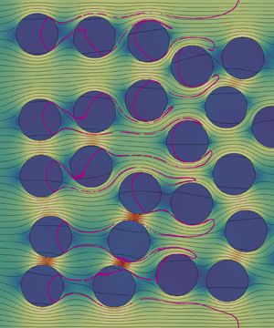
Figure 1. Flow and transport domain and streamlines of the Darcy flow  $\boldsymbol {q}({\boldsymbol {x}})$ for (a) regular and (b) random packing considering no flow boundary conditions at the top and bottom boundaries. Streamlines that cross at least one inclusion are green. Red streamlines do not go through any inclusion. In the regular media streamlines either cross all the inclusions in the horizontal or none of them. In the random media almost all streamlines cross at least one inclusion.
Packings are characterized by the domain size  $L_{x} \times L_{y}$, inclusion radius and covered volume fraction. In regular packings the inclusions needed to cover the desired area are placed in a uniform equispaced grid inside the domain (figure 1a). Random packings are generated by drawing the centres coordinates from a uniform distribution and discarding inclusions that overlap previously existing ones. The algorithm stops when the desired volume fraction is covered. This method generates arrangements with an exponential distribution of distances between inclusions (figure 1b).
2.1. Flow
We consider steady state flow through the medium described by the Darcy equation
 \begin{equation} \boldsymbol{q}({\boldsymbol{x}}) = - K({\boldsymbol{x}}) \boldsymbol{\nabla} h({\boldsymbol{x}}), \end{equation}
where  $K({\boldsymbol {x}})$ is the hydraulic conductivity, $h$ is the piezometric head and $\boldsymbol {q}$ is Darcy velocity. Both medium and fluid are assumed to be incompressible, which implies that $\boldsymbol {\nabla }\boldsymbol {\cdot }\boldsymbol {q}({\boldsymbol {x}}) = 0$. A constant flow rate $q_0$ is imposed on the left domain boundary and constant head on the right one so that the mean flow direction is along the $x$ axis.
2.1.1. Flow distribution
We discuss briefly here the flow distribution between the matrix and the inclusions which will give us some information with which to analyse the transport in the following sections.
For a single inclusion embedded in an infinite matrix, flow inside the inclusion is uniform and aligned with the mean flow direction. The ratio between undisturbed background flow velocity and the flow velocity in the inclusion is given by (Wheatcraft & Winterberg Reference Wheatcraft and Winterberg1985)
 \begin{equation} \frac{q_{in}}{q_0} = \frac{2 \kappa}{1+\kappa}, \end{equation}
where  $\kappa = K_i/K_m$ is the conductivity ratio.
For the composite media under consideration here, flow inside the inclusions is in general not perfectly uniform and is not aligned with the mean flow direction as shown in figure 1. To estimate the background flow velocity for small conductivity ratio under consideration, flow through the inclusions may be disregarded compared to the flow through the matrix. Thus, we can approximate the average flow velocity in the background
 \begin{equation} q_m = \frac{q_0}{1 - \chi}, \end{equation}
where  $\chi$ denotes the volume fraction of the inclusions.
2.2. Transport
We consider purely advective transport, which is governed by the following Liouville equation for the concentration  $c({\boldsymbol {x}},t)$:
 \begin{equation} \frac{\partial c({\boldsymbol{x}},t)}{\partial t} + \boldsymbol{v}({\boldsymbol{x}}) \boldsymbol{\cdot} \boldsymbol{\nabla} c({\boldsymbol{x}},t) = 0, \end{equation}
where  $\boldsymbol {v}({\boldsymbol {x}}) = \boldsymbol {q}({\boldsymbol {x}}) / \phi$. For simplicity, porosity $\phi$ is assumed to be constant in this work. Note that this is generally not true, particularly for geological media. However, porosity in different materials varies typically between $0.05$ and $0.4$, and this variation is much lower than that of hydraulic conductivity, which may vary over several orders or magnitude between different materials (Bear Reference Bear1972). Solute is initially uniformly distributed along a line $c({\boldsymbol {x}},t = 0) = c_0 \delta (x)$.
The transport problem is solved in a Lagrangian framework. The equation of motion for the position  ${\boldsymbol {x}}(t;\boldsymbol {a})$ of a fluid particle is
 \begin{equation} \frac{\textrm{d} {\boldsymbol{x}}(t;{\boldsymbol{a}})}{\textrm{d}t} = \boldsymbol{v}[{\boldsymbol{x}}(t;{\boldsymbol{a}})], \end{equation}
with  ${\boldsymbol {x}}(t=0;{\boldsymbol {a}}) = {\boldsymbol {a}}$. The distribution of initial positions is $\rho ({\boldsymbol {a}}) = \delta (a_1)$. In the following transport will be analysed in terms of the arrival time distribution of particles at increasing distances from the inlet.
For a medium with impermeable inclusions, macrotransport can be described by the advection dispersion equation (ADE)
 \begin{equation} \frac{\partial \bar{c}(x,t)}{\partial t} + v_a \frac{\partial \bar{c}(x,t)}{\partial x} - D_{a} \frac{\partial \bar{c}(x,t)}{\partial x^2} = 0, \end{equation}
where  $v_a$ is the apparent velocity and the dispersion coefficient $D_{a}$. For the condition of a low density of inclusions, i.e. $\chi \ll 1$, Eames & Bush (Reference Eames and Bush1999) report
 \begin{equation} D_{a} = 0.74 \chi v_{0} r_{0} \end{equation}
for impermeable inclusions and
 \begin{equation} D_{a} = \frac{8}{3{\rm \pi}\kappa} \chi v_{0} r_{0} \end{equation}
in the limit of  $\kappa \to 0$.
The distribution of arrival times at a position  $x_{c}$ for an instantaneous injection into the flux at $x = 0$ is given by Ogata & Banks (Reference Ogata and Banks1961) and Kreft & Zuber (Reference Kreft and Zuber1978) as
 \begin{equation} f(t,x_{c}) = \frac{x_{c} \exp\left[- (x_{c}-v_{a} t)^2/4 D_{a} t \right]}{\sqrt{4 D_{a} t^3}}. \end{equation}
For the complementary cumulative arrival time distribution, we obtain accordingly
 \begin{align} F(t,x_{c}) = \int_t^\infty \textrm{d}t'\, f(t',x_{c}) = 1-\frac{1}{2} \left[\text{erfc}\left(\frac{x_{c} - v_{a} t}{\sqrt{4 D_{a} t}}\right) + \exp\left(\frac{x_{c} v_{a}}{D_{a}}\right)\text{erfc}\left(\frac{x_{c}+v_{a}t}{\sqrt{4 D_{a} t}}\right)\right]. \end{align}
We use these solutions in the following as references for the observed arrival time distributions. Furthermore, we estimate the apparent velocity  $v_{a}$ and apparent dispersion coefficient $D_{a}$ from the mean $m_{b}$ and variance $\sigma _{b}^{2}$ of the breakthrough time by using the Fickian relations
 \begin{equation} v_{a} = \frac{x_{c}}{m_{b}}, \quad D_{a} = \frac{v_{a}^{3}\sigma_{b}^{2}}{2 x_{c}}. \end{equation}
2.3. Numerical model
The rectangular domain of size  $L_{x} \times L_{y}$ is discretized using square cells of side $\varDelta = r_{0}/30$. This discretization ensures that the circular shape of the inclusions is well reproduced. To avoid boundary effects the horizontal dimension is extended a buffer length $\lceil 4r_{0} \rceil$ equally distributed between the left and right boundaries.
Steady state flow (2.1) is solved using a two-point flux finite volume scheme. Uniform velocity  $v_{0}$ is prescribed on the left boundary and head on the right boundary. The top and bottom boundaries are periodic. Velocity is calculated on the cell sides.
The advection equation (2.4) is integrated using the semi-analytical method of Pollock (Reference Pollock1988). At the beginning of the simulation  $N_{p} = 10^{6}$ particles are uniformly distributed along the left boundary. The buffer between the boundary and the first inclusions ensures that flow is uniform and the streamlines parallel at the inlet. Therefore the uniform distribution of particles is equivalent to a flux-weighted injection. The simulation runs until all particles leave the domain. Streamlines and equivalently particle trajectories are illustrated in figure 1.
Results are reported in dimensionless units. We chose as characteristic length the side of the unit cell  $\ell _{c}$ of a regular arrangement with inclusions of radius $r_{0}$ that covers a volume fraction $\chi$ (figure 2). That is, $\ell _{c}= r_{0}\sqrt {{\rm \pi} /\chi }$. The characteristic time is $\tau _{c} = \ell _{c}/v_{0}$ so that a dimensionless time of one is required to traverse the unit cell at the prescribed velocity. The time needed to travel through the buffer area is subtracted from the results.
Figure 2. Sketch of the set-up for a unit cell of size  $\ell _{c}$ containing an inclusion of radius $r_{0}$. Only particles in the segment $b$ enter the inclusion.
3. Transport behaviour
We study the transport behaviour in media with random arrangements of inclusions. Transport is characterized by the travel time of the particles in terms of the breakthrough curve or equivalently by the complementary cumulative breakthrough curve at control planes. We will also analyse the trapping events distribution (i.e. the number of inclusions that a particle is transported through before arriving at the control plane), and the velocity distribution inside the inclusions. The velocity in the background material does not vary much. However, the tortuosity of the flow paths leads to an enhanced spreading of the particles as discussed for macrodispersion.
3.1. Single inclusion
We consider first the case of a medium in which there is only one inclusion of low permeability (see figure 2). We analyse the residence time of the particles within the inclusion and the relation with the breakthrough curve.
3.1.1. Residence times
The residence time distribution in a single inclusion in an infinite domain is obtained by purely geometrical considerations as follows. The flow field within an isolated single inclusion is constant. Since the streamlines inside the inclusion are parallel, the particles that go through it are uniformly distributed over the vertical diameter. This means that the vertical particle position is uniformly distributed in  $[-r_{0},r_{0}]$. The position $h$ of a particle on the vertical diameter of the inclusion is $h = r_{0} \sin \alpha$. Therefore, we obtain the angle $\alpha$ at which the particle entered the inclusion as
 \begin{equation} \alpha(h/r_{0}) = \arcsin{(h/r_{0})}. \end{equation}
From this we obtain the angular distribution that corresponds to the uniform particle distribution as
 \begin{equation} p_\alpha(\alpha) = \cos{\alpha}. \end{equation}
The length of the circle segment traversed by the particle  $l_i$ is given by $s(\alpha ) = 2 r_{0} \cos {\alpha }$, whose distribution $p_{l_{i}}(l_{i})$ is obtained from $p_\alpha (\alpha )$ as
 \begin{equation} p_{l_{i}}(l_{i}) = p_\alpha[\arccos{(l_{i}/2r_{0})}] \left.\frac{1}{\textrm{d}l_{i}(\alpha)/\textrm{d}\alpha}\right|_{\alpha = \arccos{(l_{i}/2r_{0})}}. \end{equation}
Thus,
 \begin{equation} p_{l_{i}}(l_{i}) = \frac{l_{i}}{r_{0}} \frac{1}{\sqrt{1 - (l_{i}/2r_{0})^2}}, \end{equation}
and the distribution of transition times  $t = l_{i}/v_{in}$ is given by
 \begin{equation} \psi(t) = \frac{t}{\tau_{in}^2} \frac{1}{\sqrt{1 - (t / \tau_{in})^2}}, \end{equation}
where we defined  $\tau _{in} = 2r_{0}/v_{in}$ is the maximum advection time across the inclusion. The comparison between (3.5) and residence times obtained numerically is shown in figure 3.
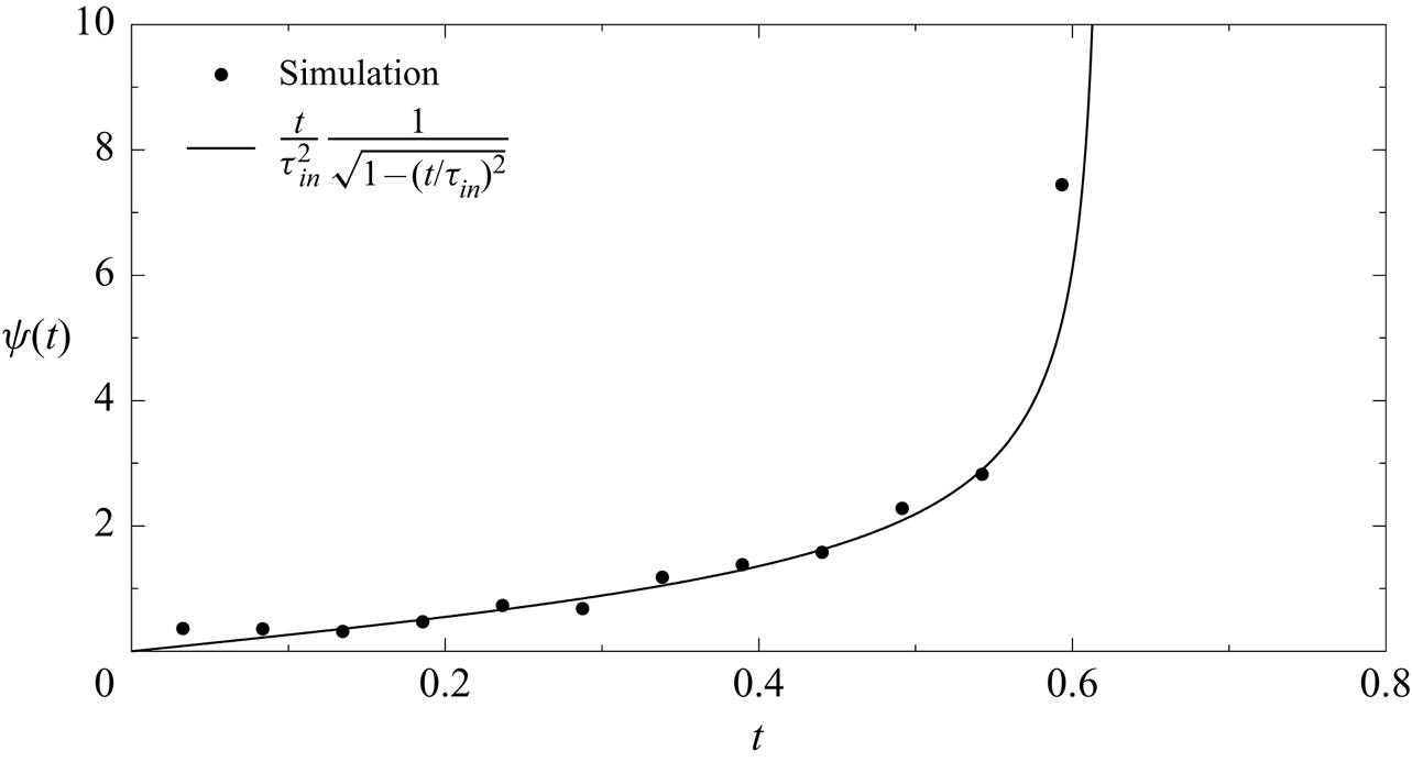
Figure 3. Comparison between the simulated (dots) and analytical (solid line) residence time distribution of particles travelling through a single inclusion (3.5)  $(\chi =0.01$ and $\kappa = 0.1)$.
3.1.2. Fraction of particles traversing the inclusion
The fraction of particles entering over a length  $\ell _c$ that traverses through the inclusion is obtained from flux conservation. The size $b$ of the streamtube in the matrix passing through the inclusion is obtained from
 \begin{equation} 2 r_{0} v_{in} = b v_m. \end{equation}
Thus, the flux proportion that goes through the inclusion can be written as
 \begin{equation} a_0 = \frac{b}{\ell_{c}} = \frac{2 r_0 v_{in}}{\ell_{c}v_m} = \frac{4 r_0}{\ell_c} \frac{\kappa}{1 + \kappa}, \end{equation}
where we used expression (2.2).
3.1.3. Breakthrough curves
The breakthrough and the complementary cumulative breakthrough curves for the single inclusion are shown in figure 4. The first arrival occurs at  $t=1$, which corresponds to the time needed to go through the unit cell. Part of the streamlines are bent by the presence of the low permeability inclusion causing the peak to widen. The rest of the curve reflects the effect of the low permeability inclusion with a breakthrough curve (figure 4b) that follows the above calculated residence time distribution.

Figure 4. Breakthrough curve (a) and complementary cumulative breakthrough curve (b) for a system containing one inclusion ( $\chi =0.01$, $\kappa = 0.1$) measured at a distance $\ell _{c}$ from the inlet. The curves show an early arrival of particles that only travel through the matrix and a long tail formed by the particles traversing the inclusion at different heights.
Transport through a single inclusion can be conceptualized as a streamtube model with two types streamtubes. In one of them, a percentage of particles  $a_{0}$ (3.7) is transported through the inclusion, while in the other one particles are transported only through the matrix. This conceptual model can be extended to regular packings whose unit cell contains only one inclusion. In this case particles will either travel through all the inclusions in the streamtube or none of them (see figure 1). The travel times inside of each streamtube are distributed due to the tortuosity of the streamlines. For regular packings the streamlines differ from the single inclusion case because of the finite size of the unit cell, which enforces a straight streamline at its boundary.
Based on the conceptual model of two streamtubes and considering that the inclusions are much less permeable than the background, the breakthrough curve is characterized by two distinct pulses caused by transport in the streamtubes without and with inclusions (figure 4). Note that the transition is continuous, as the outermost streamlines of the two streamtubes coincide.
For short media, the periodic medium could be a useful approximation to predict breakthrough curves. Zinn et al. (Reference Zinn, Meigs, Harvey, Haggerty, Peplinski and von Schwerin2004) carried out experiments of solute transport in two-dimensional glass bead packs, where circular inclusions were randomly placed into a less permeable background. They used the streamtube approach to predict breakthrough curves for the advective dominated case. As the approximate solution is based on one single inclusion, periodicity is inherently assumed. In the measured breakthrough curves, the double breakthrough behaviour is very clear and it could be demonstrated that their streamtube approach worked well to reproduce the breakthrough curves (see also next subsection).
3.2. Random packings
We consider now random packings of inclusions generated as explained in § 2. First we consider media of different sizes ( $3 \le L_{x}/\ell _{c} \le 500$; $1 \le L_{y}/\ell _{c} \leq 105$) and covered volume fraction ( $0.1 \le \chi \leq 0.55$) in which we study the velocity distribution in the matrix and inclusions, the trapping events experienced by particles and the trapping time distribution.
Then we study the behaviour of breakthrough curves. First we explore further the streamtube model using the geometry of Zinn et al. (Reference Zinn, Meigs, Harvey, Haggerty, Peplinski and von Schwerin2004). Next we consider two scenarios, a long medium ( $387\ell _{c} \times 3.8\ell _{c}$) in which transport is analysed as the distance from the inlet increases, and a wide medium ( $84\ell _{c} \times 28\ell _{c}$) in which the effect of the length of the line along which solute is injected is studied.
3.2.1. Velocity distribution
The velocity inside isolated regularly arranged inclusions is approximately constant under low density of inclusions conditions, this means for  $\chi \ll 1$. For increasing $\chi$ in random packing this is in general not the case and flow velocities vary inside the inclusions and between inclusions. We characterize the inclusions by their mean velocities, and study their distributions $p_v(v)$ as a function of volume fraction $\chi$. Figure 5 shows the distributions of inclusion velocities for different volume fractions and inclusion sizes. We observe that the distribution of mean velocities can be well approximated by a log-normal distribution. Consistent with (2.2) and (2.3), the mean velocity of the distribution is independent of the inclusion size and depends only on the volume fraction $\chi$ for constant $\kappa$. The distribution becomes narrower with decreasing $\chi$. In fact, in the limit of low density of inclusions, $p_v(v)$ should converge to the Delta distribution $p_v(v) = \delta (v-v_{in})$, where $v_{in}$ is the constant velocity in a single isolated inclusion.
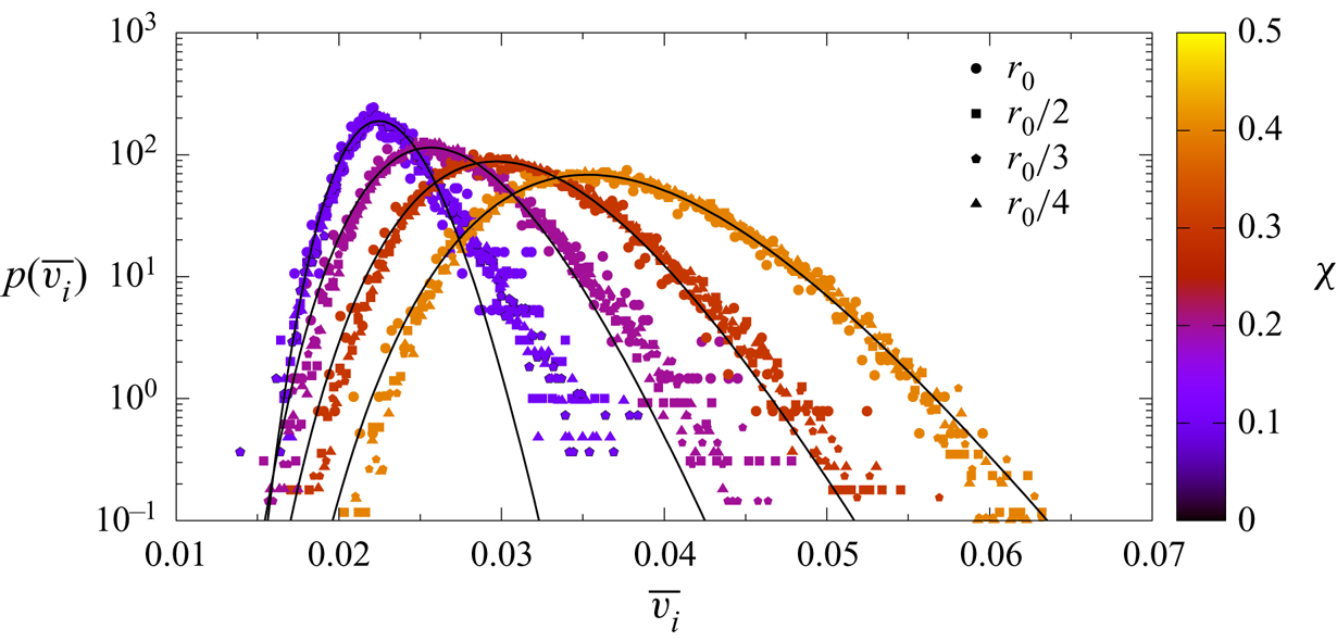
Figure 5. Mean velocity distribution inside the inclusions (symbols) for a media with varying volume fraction and inclusions’ size with constant  $\kappa = 0.01$. The solid lines show the fit to a log-normal distribution to the all the data with same $\chi$. The base case geometry is $L_{x}=49.7\ell _{c}$, $L_{y}=2.5\ell _{c}$ and $\chi =0.1$. The rest of the cases have the same domain proportions.
The velocity in the matrix (figure 6) is inversely proportional to the covered area ratio  $\chi$ and follows the relation (2.3) until a high volume fraction is covered, reaching the percolation threshold, and the hypothesis that flow through the inclusions is negligible compared to the flow through the matrix is no longer valid.

Figure 6. Mean velocity in the matrix versus volume fraction occupied by the inclusions. The solid line corresponds to the solution (2.3) for isolated inclusions. Dot colours correspond to the medium length.
3.2.2. Trapping events
The number of trapping events experienced by a particle in random media is not binary distributed as in the regular ones. As the inclusions are randomly distributed in space, the distance between them is approximately an exponential distribution, or in other words, the number of inclusions that may be encountered within a given distance follows a Poisson process (Feller Reference Feller1968). In fact, we find that the statistics of the number  $n_{tr}$ of trapping events within a travel distance $\ell$ can be described by the Poisson distribution
 \begin{equation} p(n_{tr},\ell) = \frac{\textrm{e}^{-k\ell}\left(k \ell\right)^{n_{tr}}}{n_{tr}!}. \end{equation}
An example of the trapping events distributions is shown in figure 7. It can be seen that the distribution of trapping events evolves as the particles sample the medium. At short distance from the inlet the distribution is narrow suggesting that for a small medium the streamtube approximation could be sufficient to explain transport. As the distance from the inlet increases, the distribution widens and the probability of not being trapped decreases. At a sufficient travel distance all particles experience at least one trapping event and the distribution converges to a Poisson distribution.

Figure 7. Distribution of number of trapping events (symbols) at different distances  $x_{c}$ from the inlet for an arrangement of inclusions ( $L_{x}=387\ell _{c}$, $L_{y}=3.87\ell _{c}$, $\kappa = 0.01$, $\chi =0.3$; same as in figure 11). The solid lines are the fit to a Poisson distribution.
The trapping rate  $k$, that is the number of trapping events per travelled distance, that characterizes the Poisson distribution depends on the geometry of the arrangement. To assess this dependence we performed a series of simulations varying the medium geometry (radius, length, width and area covered by the inclusions). The average distance between the inclusions $d$ was computed with the following algorithm. First, we take the lines between all pairs of inclusions’ centres that do not intersect another inclusion. Then, for every pair of lines that intersect, the shortest one is kept. Finally, the average length of the remaining lines is calculated. As shown in figure 8 the trapping rate is inversely proportional to the average distance between the inclusion $d$, expressed in terms of the unit cell size $\ell _{c}$.

Figure 8. Trapping frequency (parameter in Poisson distribution) versus mean distance between inclusions. Point colour is the covered volume fraction  $\chi$.
3.2.3. Distribution of trapping times
The trapping time distribution is obtained numerically from the residence time distribution in a single inclusion (3.5). The distribution of trapping times in the following is denoted by  $\psi _{f}(t)$. It can be constructed from the distribution $\psi (t|v)$ of trapping times for a given inclusion velocity, and the distribution $p_v(v)$ of velocities as
 \begin{equation} \psi_f(t) = \int_0^\infty \textrm{d} v\, p_v(v) \psi(t|v). \end{equation}
Figure 9 compares the distribution of trapping times obtained from the direct numerical simulations and the model (3.9).

Figure 9. Comparison between the theoretical trapping times distribution given by (3.9) (black line) and the numerical results for media with  $L_{y}=3.87\ell _{c}$, $\kappa = 0.01$, $\chi =0.3$ and different lengths (symbols).
3.2.4. Breakthrough curves
We consider first a medium based on the inclusions geometry of Zinn et al. (Reference Zinn, Meigs, Harvey, Haggerty, Peplinski and von Schwerin2004). This medium has  $\chi = 0.37$, $L_{x}= 10.8\ell _{c}$ and $L_{y} = 5.4\ell _{c}$. We consider an intermediate permeability ratio scenario with $\kappa = 0.01$. The breakthrough curve (figure 10) is affected by the random arrangement of inclusions. However, we can distinguish the contribution of particles that experience different numbers of trapping events. Given the small size of the domain and the low number of inclusions, particles experience only a few trapping events and most of them travel through the domain without entering any inclusion. Based on this phenomenology, Zinn et al. (Reference Zinn, Meigs, Harvey, Haggerty, Peplinski and von Schwerin2004) used a streamtube approach in order to model the breakthrough curves observed in their experiment. Their approach identified a streamtube passing only through the matrix and a second streamtube that passes through a constant number of inclusions. This approach is not valid in a large medium characterized by a random arrangement of inclusions because streamlines may pass through random numbers of inclusions, as discussed below.

Figure 10. Breakthrough curve (a) and complementary cumulative breakthrough curve for a random medium with a geometry as in Zinn et al. (Reference Zinn, Meigs, Harvey, Haggerty, Peplinski and von Schwerin2004) ( $L_{x}= 10.8\ell _{c}$, $L_{y} = 5.4\ell _{c}$, $\kappa = 0.01$ and $\chi = 0.37$). The dashed lines correspond to the analytical solution (2.10) where $D_{a}$ and $v_{a}$ are obtained from the mean and variance of the breakthrough time.
Next we consider a long and narrow medium ( $387\ell _{c} \times 3.8\ell _{c}$), where particles can travel through a larger number of inclusions. As shown in figure 11 the shape of the breakthrough curves depends on the travelled distance, that is, the amount of medium heterogeneity sampled. The curves become smoother as the distance from the inlet increases. For short distances (figure 11a,d) the first part of the curve is dominated by the dispersion caused between the streamlines along the fast paths and the tail of the curve by the streamlines going through the inclusions as in the case of the geometry of Zinn et al. (Reference Zinn, Meigs, Harvey, Haggerty, Peplinski and von Schwerin2004). For a sufficiently long distance from the inlet (figure 11b,c,e,f), the shapes of the breakthrough curves suggest that the peak and tail behaviour can be modelled by an effective hydrodynamic dispersion coefficient. The parameters of the apparent centre of mass velocity and dispersion coefficients are obtained from the breakthrough data according to (2.11a,b). Their values are given in table 1.
Figure 11. Breakthrough curves (a–c) and complementary cumulative breakthrough curves (d–f) at different distances from the inlet for a random arrangement of inclusions ( $L_{x}=387\ell _{c}$, $L_{y}=3.87\ell _{c}$, $\kappa = 0.01$, $\chi =0.3$). The dashed lines correspond to the analytical solution (2.10) where $D_{a}$ and $v_{a}$ are given in table 1. Note that the cases $x_{c} = \ell _{c}, 5\ell _{c}$ are not modelled.
Table 1. Values of velocity  $v_{a}$ and dispersion coefficient $D_{a}$ are determined from the mean and variance of the corresponding breakthrough times. For comparison the values predicted by Eames & Bush (Reference Eames and Bush1999) are $D_{a}= 0.0686$ for impermeable inclusions and $D_{a} = 7.87$ for $\kappa \ll 1$.
The average velocity fluctuates little, and is close or equal to the velocity set by the flow boundary condition. The dispersion coefficient is variable and evolves with distance from the inlet plane. The corresponding Fickian solutions (2.9) and (2.10) provide good descriptions of the breakthrough curves at large distances ( $x_{c} > 300 \ell _{c}$, figure 11c,f) from the inlet plane. However, the dispersion coefficients differ from the ones obtained by Eames & Bush (Reference Eames and Bush1999) for impermeable inclusions (2.7), $D_{a}= 0.069$, and in the limit $\kappa \to 0$ (2.8), $D_{a} = 7.87$. As pointed out by Eames & Bush (Reference Eames and Bush1999), their expressions are valid in the low density of inclusions limit of $\chi \ll 1$, which is not the case for the volume fractions under consideration here. The fact that the inclusion velocities are distributed, as discussed in § 3.2.1, is a manifestation of the interaction between inclusions, this means, they cannot be considered isolated.
In summary, while the Fickian solution fits the peaks and part of the tails at intermediate and large distances from the inlet plane ( $x_c > 50 \ell _c$), it fails to reproduce the sharp cutoffs at early and late times, and completely fails to reproduce the breakthrough curves at short distances ( $x_c < 10 \ell _c$). Furthermore, the apparent dispersion coefficients fitted to the data evolve with distance from the inlet plane, which cannot be accommodated by a standard Fickian model based on constant transport parameters.
In order to study the impact of the width of the initial particle distribution on heterogeneity sampling we performed another series of simulations in a wide medium ( $84\ell _{c} \times 28\ell _{c}$) in which we considered injection lines of increasing length (from $0.28\ell _{c}$ to the whole width of the medium; centred at $L_{y}/2$) and computed the breakthrough curves at different distances from the inlet. The breakthrough curves (figure 12) show that injection lines of small length (figure 12a,b with injection lines of length $0.28\ell _{c}$ and $1\ell _{c}$, respectively) do not sample enough of the medium variability even at the maximum travelled distance simulated. The curves have distinct peaks/bumps, whose number increases with the distance as the number of trapping events experienced by the particles grows. This behaviour is similar to the streamtube behaviour observed for the long medium (figure 11) and in the geometry of Zinn et al. (Reference Zinn, Meigs, Harvey, Haggerty, Peplinski and von Schwerin2004) (figure 10). For injection lines of length above $5\ell _{C}$ (figure 12c,d), the medium properties are better sampled and the shape of the curves are more similar between injections. The shape and number of peaks/bumps is less dependent on the travelled distance and only the tail of the curve changes. Note that the medium is not long enough to observe the asymptotic behaviour of figure 11(d).

Figure 12. Breakthrough curves at different distances from the inlet for injection lines of increasing length ((a,d)  $0.28\ell _{c}$, (b,e) $5\ell _{c}$ and (c,f) $28\ell _{c}$) for a medium with $L_{x} = 84\ell _{c}$, $L_{y} = 28\ell _{c}$, $\kappa = 0.01$ and $\chi =0.2$).
4. Upscaled transport model
We derive an upscaled model for transport through random packings. Unlike regular packings, in which streamtubes traverse either the same number of inclusions or none of them, in random packings streamtubes can sample a random number of inclusions. This means, one cannot distinguish only two kinds of streamtubes, but one has a set of streamtubes, each of which is characterized by different random numbers of inclusions. The analysis of § 3.2 has shown that the number of trapping events, this means, the number of inclusions a particle crosses along a trajectory, can be represented by the Poisson distribution (3.8) characterized by the trapping rate  $k$.
$k$.
Based on these observations, we can now quantify the upscaled particle motion using a CTRW framework (Berkowitz et al. Reference Berkowitz, Cortis, Dentz and Scher2006; Noetinger et al. Reference Noetinger, Roubinet, Russian, Le Borgne, Delay, Dentz, De Dreuzy and Gouze2016). To this end, we consider advective–dispersive particle transitions in the mobile matrix
 \begin{equation} \textrm{d}x(s) = v_{m} \,\textrm{d}s +\sqrt{2D_m \,\textrm{d}s}\, \xi(s), \end{equation}
where  $s$ denotes the mobile time spend outside the inclusions, $v_{m}$ is the mean velocity in the matrix, $D_{m}$ is the longitudinal dispersion coefficient, $\xi (s)$ is a Gaussian white noise characterized by zero mean and unit variance. In the model, $v_{m}$ can be estimated from the covered area $\chi$ (figure 6) and $D_{m}$ is taken equal to the dispersion coefficient for impermeable inclusions (2.7). During the mobile time $s$ particles encounter $n_{s}$ inclusions, where $n_{s}$ is distributed according to (3.8). The clock time $t(s)$ after the mobile time $s$ has passed is given by
 \begin{equation} t(s) = s + \sum_{i = 1}^{n_{s}} \tau_{i}, \end{equation}
where  $n_{s}$ is Poisson distributed with mean value $\langle n_{s} \rangle = k v_{m} s$. The trapping times $\tau _{i}$ are defined by (see appendix A)
 \begin{equation} \tau_{i} = \frac{\ell_{i}}{v_{i}} - \frac{\ell_{i}}{v_{m}}, \end{equation}
where the distance  $\ell _{i}$ is the secant of the circular inclusion at the height where the particle enters the inclusion (figure 2). It is distributed according to (3.4). The velocity $v_{i}$ in the inclusion is assumed to be constant and lognormally distributed (see § 3.2.1 and figure 5). The trapping time denotes the time a particle spends in the inclusion minus the time it would take to traverse the inclusion with the mean velocity $v_{m}$. Thus, it quantifies the net impact of the inclusion. The medium is considered ergodic if each particle samples the same distribution $\psi _{f}(t)$ of trapping times as it moves through the medium. This property is clearly not fulfilled for a periodic medium and depends on the medium and injection line length in random media. According to the above, the clock time $t(s)$ is a compound Poisson process (Feller Reference Feller1968; Margolin, Dentz & Berkowitz Reference Margolin, Dentz and Berkowitz2003; Benson & Meerschaert Reference Benson and Meerschaert2009; Comolli et al. Reference Comolli, Hidalgo, Moussey and Dentz2016). Thus, its distribution $\psi (t)$ can be written in Laplace space as (see also appendix A)
 \begin{equation} \psi^{\ast}(\lambda|s) = \exp\left(- \lambda s - k s v_m \left[1 - \psi^{\ast}_{f}(\lambda) \right] \right), \end{equation}
where Laplace transformed quantities are marked by an asterisk, and  $\lambda$ denotes the Laplace variable. Equations (4.1a)–(4.1d) constitute and upscaled CTRW model combined with a multi-trapping approach. In the following, we discuss the equivalent formulation in terms of a time non-local partial differential equation that describes advective mobile–immobile mass transfer.
In appendix A, we derive for the mobile, this means non-trapped, solute concentration  $c_m(x,t)$ the governing equation
 \begin{equation} \frac{\partial c_{m}(x,t)}{\partial t} + \frac{\partial}{\partial t} \int_{0}^{t} \textrm{d}t'\,\varphi(t - t') \gamma c_{m}(x,t') + v_{m} \frac{\partial c_{m}(x,t)}{\partial x} - D_{m} \frac{\partial^{2} c_{m}(x,t)}{\partial x^{2}} = 0, \end{equation}
where the trapping rate is given by  $\gamma = k v_m$. The memory function $\varphi (t)$ is given explicitly in terms of the advective trapping time distribution $\psi _{f}(t)$ as
 \begin{equation} \varphi(t) = \int_{t}^{\infty} \textrm{d}t'\, \psi_{f}(t'). \end{equation}
The trapping time distribution  $\psi _{f}(t)$, defined in (3.9), is determined by the inclusion size and flow velocities within the inclusions. This means, it is fully quantified in terms of the microscopic advective trapping mechanisms. The memory function (4.2b) denotes the probability that the trapping time is larger than the time $t$. Thus, we can define the immobile concentration $c_{im}(x,t)$ as
 \begin{equation} c_{im}(x,t) = \int_{0}^{t} \textrm{d}t'\, \varphi(t - t') \gamma c_m(x,t'). \end{equation}
This equation reads as follows. The immobile concentration is equal to the probability that a particle gets trapped in the immobile region at any time  $t' < t$ times the probability that the trapping time is smaller than $t - t'$. Note that in the special case of a single advection time scale $\tau _a$, this means for $\psi _f(t) = \delta (t - \tau _a)$, the memory function (4.2b) reduces to a step function as considered in Ginn et al. (Reference Ginn, Schreyer and Zamani2017).
The upscaled model defined by (4.2a)–(4.2c) is equal in form to memory function formulations of (multirate) mobile–immobile mass transfer (Haggerty & Gorelick Reference Haggerty and Gorelick1995; Carrera et al. Reference Carrera, Sánchez-Vila, Benet, Medina, Galarza and Guimerà1998; Dentz & Berkowitz Reference Dentz and Berkowitz2003; Schumer et al. Reference Schumer, Benson, Meerschaert and Baeumer2003; Ginn et al. Reference Ginn, Schreyer and Zamani2017), and defines the immobile concentration in terms of the memory function  $\varphi (t)$ as expressed by (4.2c). The memory function here quantifies advective mass transfer between high and low conductivity regions, and is fully defined in terms of the advective trapping mechanisms, inclusion size and velocity distribution. The formulation (4.2a)–(4.2c) of the upscaled model in terms of the non-local partial differential equation can be considered as an advective mobile–immobile mass transfer model.
Before we apply this model to the data of the direct numerical simulations, some comments on its assumptions are in order. The basis of the model is the assumption of ergodicity of the underlying disorder in the following sense. First, the CTRW samples the number  $n_{s}$ of trapping events from a Poisson distribution. This implies that the inclusion pattern is random and fluctuates on a characteristic length scale. All particles sample from the same Poisson distribution, this means all particles must have access to the same statistics as they move through the medium, which means that the spatial pattern needs to be stationary. The same holds for the distribution of trapping times, which are sampled as independent identically distributed random variables. In the following, we analyse the breakthrough curves in the light of these remarks.
Figure 13 compares the results for the breakthrough curves of the direct numerical simulations to the prediction of the CTRW for a narrow medium of  $L_y = 3.8 \ell _{c}$ at different distances from the inlet. This medium has in average 2.5 inclusions per vertical cross-section. For this case, we do not expect that the upscaled model provides a good prediction at short distances because the ergodicity conditions discussed above do not apply. All the particles in the direct numerical simulation initially experience the same or similar disorder, this means they are not independent statistically. In fact, transport can be interpreted as occurring in streamtubes as discussed above. Only with distance from the inlet, particles start sampling the medium structure and heterogeneity. This means in terms of the number of times particles pass an inclusion, and the trapping times experienced. Remarkably, sampling is sufficiently efficient due to the random nature of the medium that the upscaled CTRW model reproduces the primary peak of first arrival and secondary peaks that correspond to different numbers of trapping events. This means, particles sample along single streamlines a representative part of the medium statistics.

Figure 13. Comparison of the breakthrough curves (a–c) and complementary cumulative breakthrough curves (d–f) of the CTRW model (4.1) (solid lines) to the numerical simulations (dots) for a random arrangement of inclusions with  $L_{x}=387 \ell _c$, $L_{y}=3.8 \ell _c$, $\kappa = 0.01$ and $\chi =0.3$. The curves are measures at increasing distance from the inlet. The CTRW models uses the parameters (velocity in the matrix, mean number of trapping events) measured at the outlet. The mean number of trapping events is rescaled for the intermediate distances.
The breakthrough curves shown in figure 14 are measured in a medium whose lateral extension comprises  $28 \ell _c$, this means, the particles injected over the medium cross-section sample from the start a representative part of the medium heterogeneity, both in terms of the spatial structure and in terms of the trapping time statistics. Thus, the upscaled CTRW model predicts the direct simulation data already at short distances from the inlet. It provides good predictions for the first arrival, and also, as in figure 13 for the secondary peaks.

Figure 14. Comparison of the breakthrough curves (a) and complementary cumulative breakthrough curves (b) of the CTRW model (4.1) (solid lines) to the numerical simulations (dots) for a random arrangement of inclusions with  $L_{x} = 84\ell _{c}$, $L_{y} = 28\ell _{c}$, $\kappa = 0.01$ and $\chi =0.2$ for an injection line of size equal to the domain height. The curves are measured at different distances from the inlet.
5. Conclusions
We studied in this paper the advective transport of solutes in an idealized heterogeneous porous medium consisting of a homogeneous background material with low permeability circular inclusions. In such media the distribution of flow, and solute if injected uniformly, between the matrix and the low permeability inclusions is given by the permeability ratio provided that the inclusion density is not very high. While velocity in the matrix depends on fraction of the area covered by the inclusions, the mean velocity in the inclusions follows a log-normal distribution.
Transport is characterized by breakthrough curves whose shape evolves as the medium is sampled. At short distance from the injection inlet, or when the injection length is smaller than the domain, the breakthrough curve has a wavy shape that reflects the trapping of particles at the inclusions. This curve can be interpreted as transport through streamtubes with different velocities. As the distance, or injection length, grows, the properties of the medium are better sampled and the curve becomes smoother. Particles arrive gradually at the control plane, which reflects the tortuosity of the streamlines that go through the matrix. The better sampling of the velocity distribution in the inclusions makes the tail of the curve also smoother. These features are common to the behaviour of the ADE (2.6). However, the shape of the curves cannot be predicted with a macrodispersion coefficient. The ADE overestimates concentration at early times and underestimates it at late times. Unrealistic values of the dispersion coefficient are obtained from the variance of the breakthrough times (see table 1). This is particularly accentuated when the medium is undersampled.
The problem with the representation of variable travel times as macrodispersion can be illustrated with the results of Eames & Bush (Reference Eames and Bush1999). In their analysis, the macrodispersion coefficient derived for a finite permeability ratio  $\kappa$ diverges in the limit $\kappa \to 0$. However, if the inclusions are impermeable from the beginning, the macrodispersion coefficient is finite. The latter captures the effect of tortuous streamlines in the background material. If inclusions are considered permeable and $\kappa$ is very high, the macrodispersion coefficient also captures the trapping in the inclusions. As long as the inclusions are permeable, there is a probability that solute gets into an inclusion. If inside the inclusion, solute is slowed down, which leads to a tailing of the breakthrough curve. The lower the permeability ratio, the stronger the tailing due to the longer delay time. Therefore, in the limit of a ratio of zero, the tail gets infinitely long. The effect that the probability to get into an inclusion also goes to zero does not counteract the infinitely long trapping time. As the macrodispersion coefficient is obtained from the total solute distribution in the domain, a retention in an inclusion for infinite time leads to a diverging macrodispersion coefficient. In case that the inclusions are impermeable from the beginning, there is no transport through inclusions that could cause tailing. Therefore, the macrodispersion coefficient is finite. The behaviour is inherent to assuming an advection dispersion equation for the upscaled model.
We developed an upscaled transport model using a Lagrangian framework. The main assumption of the model is that the medium structure is ergodic. Therefore the model performance improves, as the particles sample a larger part of the medium heterogeneity. This is the case either when the particles travel a long distance from the inlet or when the injection length is long, so that the medium properties are explored even at short distance from the inlet.
The CTRW model developed has solid predictability capabilities because it is parameterized by measurable medium properties. The CTRW model is parameterized by the trapping rate, which we observed can be characterized by a Poisson distribution whose trapping rate (number of trapping events per distance) is inversely proportional to the mean separation between inclusions, the velocity in the matrix, which is well approximated by a function of the area covered by the inclusions (figure 6), and the velocity distribution inside the inclusions. The mean velocity inside the inclusions follows a log-normal distribution, which needs further investigation. So does the Poisson distribution of trapping events, which constitutes an important part of the upscaled model with possible applications to more general scenarios. Furthermore, we assumed constant porosity and considered a 2-D scenario. We anticipate that for 3-D geometries and variable porosity, the trapping rate and velocity distribution may change, and that otherwise the derived model remains valid.
The upscaled model was also formulated in an equivalent mobile–immobile memory function model. The memory function is determined by the trapping time distribution and for the same reasons as outlined above for the CTRW model, predictable from information about parameters and structure of the porous medium. The memory function in our setting describes tailing of breakthrough curves due to advective transport through circular inclusions with low permeability. To generalize it towards media with inclusions with a distribution of permeability values or sizes, is straight forward, if appropriate models for the velocity distribution inside of the inclusions can be formulated.
Purely advective transport was here considered as a limiting case for advective–diffusive transport. The other limiting case, purely diffusive transport inside of inclusions, has been studied and mobile–immobile models are well established for it. In a next step it would be necessary to consider the combined effect of advective and diffusive transport inside of inclusions, and to derive predictive mobile–immobile memory function models based on the models for pure advection and for pure diffusion.
Acknowledgements
Data used for producing the figures can be downloaded from digital.csic.es (https://digital.csic.es/handle/10261/216991) and by solving the respective equations. The authors thank Professor T.R. Ginn and two anonymous reviewers for their comments on the paper. J.J.H. and M.D. acknowledge the support of the Spanish Ministry of Science and Innovation (project CEX2018-000794-S and project HydroPore PID2019-106887GB-C31). J.J.H. acknowledges the support of the European Social Fund and Spanish Ministry of Ministry of Science, Innovation and Universities through the ‘Ramón y Cajal’ fellowship (RYC-2017-22300). The authors thank P. Uszes for providing the code to measure the average distance between inclusions.
Declaration of interests
The authors report no conflict of interest.
Appendix A. Upscaling
We note that the number  $n_L$ of inclusions within a distance $L$ between inlet and outlet is a Poissonian random variable. We set the average time spent mobile equal to
 \begin{equation} s = \frac{L}{v_{m}}. \end{equation}
Thus we can set  $L = v_{m} s$ and $n_s \equiv n_{L}$. Accordingly, we set the immobile time $\tau _{im}(s)$ after the mobile time $s$ has passed equal to
 \begin{equation} \tau_{im}(s) = \sum_{i = 1}^{n_{s}} \left(\frac{\ell_{i}}{v_{i}} - \frac{\ell_{i}}{v_{m}}\right), \end{equation}
where the distance  $\ell _{i}$ travelled across an inclusion are distributed according to (3.4). The inclusion velocity $v_{in}$ is lognormally distributed, see § 3.2.1. The second term under the sum compensates for the fact that the average mobile time accounts for the full distance $L$ and not only for the distance $L - \sum _{i = 1}^{n_{s}} \ell _{i}$ a particle moves in the matrix. With this reasoning, we obtain expression (4.1b) for the clock time $t(s)$.
Next we consider expression (4.1d) for the Laplace transform of the distribution  $\psi (t|s)$ of clock time $t(s)$. It can be written as
 \begin{equation} \psi(t|s) = \left\langle \delta\left(t - s - \sum_{i = 1}^{n_s} \tau_{i}\right) \right\rangle, \end{equation}
which we can expand as
 \begin{equation} \psi(t|s) = \sum_{n = 0}^\infty \left\langle \delta\left(t - s - \sum_{i = 1}^{n} \tau_{i}\right) \delta_{n,n_s} \right\rangle = \sum_{n = 0}^\infty \left\langle \delta\left(t - s - \sum_{i = 1}^{n} \tau_{i}\right)\right\rangle p_{n}(s), \end{equation}
where  $p_{n}(s)$ is the Poisson distribution
 \begin{equation} p_{n}(s) = \frac{(k v_m s)^n\exp(-k v_m s)}{n!}. \end{equation}
The Laplace transform of (A 4) is
 \begin{equation} \psi^{\ast}(\lambda|s) = \exp\left(-\lambda s \right) \sum_{n = 0}^\infty \left\langle \exp\left(-\lambda \sum_{i = 1}^{n} \tau_{i}\right)\right\rangle p_{n}(s), \end{equation}
which can be written as
 \begin{equation} \psi^{\ast}(\lambda|\ell_{c}) = \exp\left(-\lambda s \right) \sum_{n = 0}^\infty \psi_{f}^\ast(\lambda)^n p_{n}(s) \end{equation}
because the  $\tau _{i}$ are independent identically distributed random numbers. Inserting now expression (A 5) for the Poisson distribution gives
 \begin{equation} \psi^{\ast}(\lambda|s) = \exp\left(-\lambda s \right) \sum_{n = 0}^\infty \psi_{f}^\ast(\lambda)^n \frac{(k v_m s)^n \exp(-k v_m s)}{n!}. \end{equation}
The exponential sum can be evaluated explicitly and thus
 \begin{equation} \psi^{\ast}(\lambda|s) = \exp(-\lambda s - k v_m s [1 - \psi^{\ast}_{f}(\lambda)]). \end{equation}
The concentration distribution in the CTRW framework can be written as
 \begin{equation} c(x,t) = \langle \delta[t - t(s)] \rangle = \int_0^\infty \textrm{d}s\, c_0(x,s) h(s,t), \end{equation}
where we defined
 \begin{equation} c_0(x,s)\langle = \delta[x - x(s)] \rangle, \quad h(x,s) = \langle \delta[s - s(t)] \rangle. \end{equation}
The distribution  $c_0(x,s)$ satisfies the advection–dispersion equation
 \begin{equation} \frac{\partial c_0(x,s)}{\partial s} + v_m \frac{\partial c_0(x,s)}{\partial x} - D_m \frac{\partial^2 c_0(x,s)}{\partial x^2} = 0. \end{equation}
The distribution  $h(s,t)$ of the renewal process $s(t) = max(s|t(s) \leq t)$ satisfies
 \begin{equation} \int_0^s \textrm{d}s\, h(s,t) = \int_t^\infty \textrm{d}t'\, \psi(t'|s). \end{equation}
Thus, the concentration  $c(x,t)$ can be written as
 \begin{equation} c(x,t) = \int_0^\infty \textrm{d}s\, c_0(x,s) \frac{\partial}{\partial s} \int_t^\infty \textrm{d}t'\, \psi(t'|s). \end{equation}
This equation can be written in Laplace space as
 \begin{equation} c^\ast(x,\lambda) = \int_0^\infty \textrm{d}s\, c_0(x,s) \frac{\partial}{\partial s} \frac{1 - \psi^{\ast}(\lambda|s)}{\lambda}. \end{equation}
Inserting expression (A 9) for  $\psi ^{\ast }(\lambda |s)$ gives
 \begin{equation} c^\ast(x,\lambda) = \left\{\lambda + k v_m [1 - \psi^{\ast}_{f}(\lambda)] \right\} \int_0^\infty \textrm{d}s\, c_0(x,s) \psi^{\ast}(\lambda|s). \end{equation}
On the other hand, integration of (A 15) by parts gives
 \begin{align} \lambda c^\ast(x,\lambda) = - \int_0^\infty \textrm{d}s \frac{\partial c_0(x,s)}{\partial s} [1 - \psi^{\ast}(\lambda|s)] = \delta(x) + \int_0^\infty \textrm{d}s \frac{\partial c_0(x,s)}{\partial s} \psi^{\ast}(\lambda|s), \end{align}
where  $c_0(x,s=0) = \delta (x)$. Equation (A 12) implies that the right side can be written as
 \begin{equation} \lambda c^\ast(x,\lambda) = \delta(x) + \left[ + v_m \frac{\partial}{\partial x} - D_m \frac{\partial^2}{\partial x^2} \right] \int_0^\infty \textrm{d}s\, c_0(x,s) \psi^{\ast}(\lambda|s). \end{equation}
Using now expression (A 16) on the right side of this expression in order to eliminate  $c_0(x,s)$ in favour of $c^\ast (x,\lambda )$ gives
 \begin{equation} \lambda c^\ast(x,\lambda) = \delta(x) + \left[ + v_m \frac{\partial}{\partial x} - D_m \frac{\partial^2}{\partial x^2} \right] \frac{c^\ast(x,\lambda)}{\lambda - k v_m [1 - \psi^{\ast}_{f}(\lambda)]}. \end{equation}
We define now the mobile concentration  $c_m^\ast (x,\lambda )$ as
 \begin{equation} c_m^\ast(x,\lambda) = \frac{c^\ast(x,\lambda)}{\lambda + k v_m [1 - \psi^{\ast}_{f}(\lambda)]}. \end{equation}
Thus, we obtain for the mobile concentration  $c_m^\ast (x,s)$ the governing equation
 \begin{equation} \lambda c_m^\ast(x,\lambda) + \lambda \varphi^\ast(\lambda) c_m^\ast(x,\lambda) = \delta(x) + \left[ + v_m \frac{\partial}{\partial x} - D_m \frac{\partial^2}{\partial x^2} \right] c_m^\ast(x,\lambda), \end{equation}
where we defined the memory function
 \begin{equation} \varphi^\ast(\lambda) = k v_m \frac{1 - \psi^{\ast}_{f}(\lambda)}{\lambda}. \end{equation}
Furthermore, we can now define the immobile concentration  $c_{im}^\ast (x,\lambda )$ as
 \begin{equation} c_{im}^\ast(x,\lambda) = k v_m [1 - \psi^{\ast}_{f}(\lambda)] c_m^\ast(x,\lambda). \end{equation}
The inverse Laplace transform of this expression is given by (4.2b).


 Open access