


1. Introduction
Shock wave/boundary layer interactions (SWBLIs) are omnipresent in high-speed aerodynamics such as supersonic inlets, over-expanded nozzles, high-speed aerofoils and space launchers, and have received considerable attention over the past decades (Green Reference Green1970; Dolling Reference Dolling2001). It is reported widely that SWBLIs feature complex unsteady dynamics over a broadband frequency spectrum. The strong fluctuations of pressure and friction forces accompanying this flow phenomenon can induce intense localized mechanical and thermal loads, even possibly leading to the failure of material and structural integrity (Délery & Dussauge Reference Délery and Dussauge2009; Gaitonde Reference Gaitonde2015).
Although SWBLIs are observed on various types and parts of aircraft, two-dimensional SWBLIs can be abstracted into four canonical configurations: (1) incident (impinging/ reflecting) shock, (2) compression ramp, (3) backward-facing step (BFS), and (4) forward-facing step (FFS). Many efforts have been made, and much progress was accomplished by means of advanced flow measurement techniques and well-resolved numerical simulations, especially for the compression ramp and impinging shock configurations. As we can see from figure 1, typically the interaction region of those four configurations forms an approximately triangular structure, consisting of the separation shock (except for the BFS configuration), shear layer and reattachment shock (Babinsky et al. Reference Babinsky2011). However, there are some differences of the flow structures. For the impinging/reflecting shock case, the separation bubble is caused by the strong adverse pressure gradient induced by the incident shock. In the BFS case, the separation is caused by the sudden geometry expansion at the step edge. In contrast, for the compression ramp and FFS cases, the separation in these two configurations is produced by the flow compression due to the contraction of the geometry. In the published literature, including our previous work (Grilli, Hickel & Adams Reference Grilli, Hickel and Adams2013; Pasquariello, Hickel & Adams Reference Pasquariello, Hickel and Adams2017; Hu, Hickel & van Oudheusden Reference Hu, Hickel and van Oudheusden2021), the first three SWBLI geometries have been well investigated, whereas seldom has attention been paid to the FFS. In the FFS configuration, the boundary layer separates far upstream of the step and reattaches on the step wall or downstream of the step. Compression waves are generated around the separation point due to the deflection of the shear layer by the recirculating flow region. These compression waves then coalesce into a separation shock away from the wall. A second compression wave system can form in the vicinity of the step as the flow reattaches on the step wall. An expansion fan is formed as the flow turns around the step corner in the direction tangential to the upper surface. There may also be a small secondary separation and reattachment on the upper wall (Zheltovodov Reference Zheltovodov1996).

Figure 1. Mean flow structures of SWBLIs in canonical two-dimensional configurations (Babinsky et al. Reference Babinsky2011): (a) impinging shock, (b) compression ramp, (c) backward-facing step, and (d) forward-facing step. (PME stands for the Prandtl–Meyer expansion.)
For all the geometries shown in figure 1, the interaction system features large-scale unsteady motions whose frequencies are usually one or two orders lower than the boundary layer integral frequency  $u_\infty / \delta$ (Touber & Sandham Reference Touber and Sandham2009, Reference Touber and Sandham2011). Generally, there are two main groups of theories regarding the source of the low-frequency unsteadiness, which are referred to as the upstream and downstream dynamics (Clemens & Narayanaswamy Reference Clemens and Narayanaswamy2014). Theories of the former kind attribute the low-frequency motions of the shock to the velocity or pressure fluctuations within the incoming turbulent boundary layer (Plotkin Reference Plotkin1975). In extensive existing experimental and numerical studies, these upstream oscillations of flow variables have been observed in various forms, including the bursting events in the upstream boundary layer, as inferred from the pressure measurements of a compression ramp by Andreopoulos & Muck (Reference Andreopoulos and Muck1987), and elongated superstructures with low- and high-speed streaks observed in the stereoscopic/tomographic particle image velocimetry (PIV) and planar laser scattering (PLS) measurements in both the compression ramp (Ganapathisubramani, Clemens & Dolling Reference Ganapathisubramani, Clemens and Dolling2007) and the incident shock case (Humble et al. Reference Humble, Elsinga, Scarano and van Oudheusden2009). A simple linear restoring model, in which the shock is displaced by the upstream velocity fluctuations and tends to restore to its mean position driven by the stability of the mean flow, was proposed to explain the physical connection between the shock oscillations and the fluctuations inside the upstream boundary layer (Plotkin Reference Plotkin1975; Beresh, Clemens & Dolling Reference Beresh, Clemens and Dolling2002). Another model ascribes the low-frequency motions to the selective amplification/response dynamics of the separation bubble driven by certain large-scale perturbations in the upstream boundary layer (Touber & Sandham Reference Touber and Sandham2011; Porter & Poggie Reference Porter and Poggie2019).
Theories of the second kind consider the low-frequency behaviour as being determined by the downstream interaction region. There is ample evidence that the low-frequency motions of the separation shock are related to the unsteady behaviour of the separation region (Erengil & Dolling Reference Erengil and Dolling1991; Thomas, Putnam & Chu Reference Thomas, Putnam and Chu1994; Dupont, Haddad & Debiève Reference Dupont, Haddad and Debiève2006). Several hypotheses have been proposed to explain the downstream dynamics of the low-frequency unsteadiness. Touber & Sandham (Reference Touber and Sandham2009) found an unstable global mode inside the separation bubble from their global linear stability analysis, which excites a forcing source for the low-frequency unsteadiness by displacing the separation and reattachment points. Grilli et al. (Reference Grilli, Schmid, Hickel and Adams2012) propose that mixing across the separated shear layer is the main contributor to the low-frequency contraction and expansion of the separation bubble. Based on direct numerical simulations (DNS) of a Mach 2.25 impinging shock case, Pirozzoli & Grasso (Reference Pirozzoli and Grasso2006) believe that the low-frequency oscillations are caused by a resonance between the bubble and incident shock. During this process, acoustic waves are produced by the interaction between coherent structures in the bubble and the incident shock, and then these acoustic waves propagate upstream, leading to the low-frequency behaviour of the SWBLI system. Piponniau et al. (Reference Piponniau, Dussauge, Debiève and Dupont2009) proposed an entrainment-injection model to explain the underlying mechanism of the low-frequency unsteadiness. They believe that a gradual contraction of the separation bubble is caused by a continuous mass entrainment by the separated shear layer, which is then periodically compensated by a reverse mass flow that causes the dilatation of the separation bubble. This model was examined further by Wu & Martin (Reference Wu and Martin2008) in their DNS of a compression ramp. Several numerical works reported streamwise-elongated Görtler vortices originating around the reattachment location in both the impinging shock and compression ramp configurations (Grilli et al. Reference Grilli, Hickel and Adams2013; Priebe et al. Reference Priebe, Tu, Rowley and Martín2016; Pasquariello et al. Reference Pasquariello, Hickel and Adams2017). By means of dynamic mode decomposition (DMD) analysis, a group of low-frequency modes was identified that show a strong correlation of low-frequency shock dynamics with the momentum streaks induced by Görtler-like vortices (Pasquariello et al. Reference Pasquariello, Hickel and Adams2017). The Görtler instability is thus a possible forcing mechanism of the low-frequency SWBLI dynamics.
Souverein et al. (Reference Souverein, Dupont, Debiève, Dussauge, van Oudheusden and Scarano2010) proposed that the dominant mechanism of the low-frequency SWBLI depends on shock strength and Reynolds number. In a weak SWBLI, upstream effects are the main cause of the low-frequency unsteady motions, while the downstream dynamics of the separation bubble is the dominant mechanism of the unsteadiness in strong SWBLI (Clemens & Narayanaswamy Reference Clemens and Narayanaswamy2014). As indicated by Priebe et al. (Reference Priebe, Tu, Rowley and Martín2016) and Hu et al. (Reference Hu, Hickel and van Oudheusden2021), although the downstream Görtler vortices may be the possible origin of the low-frequency unsteadiness, there are still certain dependencies on the perturbation environment provided by the upstream boundary layer.
Specific to the FFS configuration, early experimental works have confirmed the low-frequency pressure and energy fluctuations in the separation region (Kistler Reference Kistler1964; Behrens Reference Behrens1971). White & Visbal (Reference White and Visbal2015) calculated the premultiplied power spectral density of the wall pressure from a numerical simulation, and found that the value of the dominant low frequency is approximately two orders lower than that of the wall turbulence. Recent PIV experiments also observed these unsteady motions of the interaction system (Zhang et al. Reference Zhang, Zhu, Yi and Wu2016). The origin of the low-frequency unsteadiness was investigated in several recent studies. By means of a correlation analysis based on PIV measurements, Murugan & Govardhan (Reference Murugan and Govardhan2016) found that the location of the separation shock is well correlated to the separation bubble area but only weakly connected to the disturbances within the upstream boundary layer. On the other hand, the compression waves around the shock foot are strongly connected to the spanwise-aligned high- and low-speed streaks in the upstream near-wall boundary layer. Therefore, they believe that the upstream three-dimensional disturbances contribute most to the low-frequency unsteadiness of the interaction system in the FFS configuration. Simonenko, Zubkov & Kuzmin (Reference Simonenko, Zubkov and Kuzmin2018) also observed the longitudinal streaks, generated by a counter-rotating vortex pair, upstream of the step in their numerical results. Estruch-Samper & Chandola (Reference Estruch-Samper and Chandola2018) proposed a physical mechanism involving both upstream and downstream effects. Different from the physical model proposed by Piponniau et al. (Reference Piponniau, Dussauge, Debiève and Dupont2009), they also take into account the response of the upstream boundary layer to the separated shear layer, and believe that the induced shear layer instabilities are independent of the downstream dynamics according to the free-interaction theory. The downstream effects are caused by the entrainment of the mass flow as the shear layer is shedding downstream, and the recharging of the separation bubble when the shear layer reattaches on the downstream wall. The frequency of the bubble breathing scales effectively as the ratio of the mass ejection rate to the reversed flow rate. Based on these observations, they believe that the separated shear layer is the main driver of the low-frequency unsteadiness.
Similar to the aforementioned studies of impinging shock and compression ramp cases, there is also no general consensus on the source of the low-frequency unsteadiness in the FFS configuration. Since the flow topology in the FFS shares many similarities with the compression ramp, one can assume that the low-frequency dynamics is governed by similar mechanisms, such as possible effects of the upstream disturbances, the counter-rotating vortices and the downstream entrainment-recharging process. However, it remains an open question whether the conclusions obtained for other configurations, including our previous work on BFS (Hu et al. Reference Hu, Hickel and van Oudheusden2021), can be applied similarly to the FFS configuration. To scrutinize the dominant mechanism of the low-frequency unsteadiness, experiments or simulations with different levels of upstream disturbances would be required at otherwise identical flow parameters. Towards this end, we perform well-resolved large-eddy simulations (LES) of two FFS flows at freestream Mach number  $Ma =1.7$ and Reynolds number $Re_{\delta _0}=13\,718$ based on the boundary layer thickness, the first with a low-perturbation laminar inflow boundary layer, and the second with a fully developed turbulent inflow boundary layer. Both cases are then analysed and compared, with special attention paid to flow structures and low-frequency dynamics in order to identify correlations and a possible physical mechanism of the low-frequency unsteadiness in supersonic FFS flows.
The paper is structured as follows. Details of the numerical methods and the set-up of the flow configuration are given in § 2. Then the flow topology of the mean and instantaneous flow is discussed in § 3. The characteristic frequencies of the significant unsteady motions are analysed using spectral analysis. Finally, dominant modes in the SWBLI are extracted via a three-dimensional DMD. By comparing the laminar and turbulent cases, a physical mechanism of the low-frequency unsteadiness source is proposed in § 4. The conclusions, with a summary of the main results, are presented in § 5.
2. Problem formulation and set-up
2.1. Governing equations
The physical problem is governed by the three-dimensional compressible Navier–Stokes equations with appropriate boundary and initial conditions, and the constitutive relations for an ideal gas. These equations are composed of the continuity, momentum and total energy equations:
 \begin{gather} \frac{\partial \rho}{\partial t}+\frac{\partial}{\partial x_{i}}(\rho u_{i})=0 , \end{gather}
 \begin{gather} \frac{\partial \rho u_{j}}{\partial t}+\frac{\partial}{\partial x_{i}}\left(\rho u_{i} u_{j}+\delta_{i j} p-\tau_{i j}\right)=0 , \end{gather}
 \begin{gather} \frac{\partial E}{\partial t}+\frac{\partial}{\partial x_{i}}\left(u_{i} E + u_{i} p-u_{j} \tau_{i j}+q_{i}\right)=0 , \end{gather}
where  $\rho$ is the density, $p$ is the pressure and $u_i$ is the velocity vector. The total energy $E$ is defined as
 \begin{equation} E = \frac{p}{\gamma-1} + \frac{1}{2}\,\rho u_i u_i . \end{equation}
The viscous stress tensor  $\tau _{i j}$ follows the Stokes hypothesis for a Newtonian fluid,
 \begin{equation} \tau_{i j} = \mu \left(\frac{\partial u_i}{\partial x_j} + \frac{\partial u_j}{\partial x_i} - \frac{2}{3}\,\delta_{i j}\,\frac{\partial u_k}{\partial x_k} \right) , \end{equation}
and the heat flux  $q_i$ is determined by Fourier's law,
 \begin{equation} q_i ={-}\kappa\,{\partial T}/{\partial x_i} . \end{equation}
 The fluid is modelled as a perfect gas with specific heat ratio  $\gamma =1.4$ and specific gas constant $R={287.05}\,{{\rm J}\,{\rm kg}^{-1}\,{\rm K}^{-1}}$, following the ideal gas equation of state
 \begin{equation} p = \rho R T . \end{equation}
The dynamic viscosity  $\mu$ and thermal conductivity $\kappa$ are functions of the static temperature $T$, and are computed according to Sutherland's law:
 \begin{gather} \mu = \mu_{ref}\,\frac{T_{ref} + S}{T + S} \left( \frac{T}{T_{ref}} \right) ^{1.5} , \end{gather}
 \begin{gather} \kappa = \frac{\gamma R}{(\gamma -1)\,Pr}\,\mu . \end{gather}
The parameter values selected for the computations are  $\mu _{ref} = 18.21 \times 10^{-6} \, \mathrm {Pa}\,\mathrm {s}$, ${T_{ref} = 293.15\,{\rm K}}$, $S={110.4}\,{{\rm K}}$ and $Pr = 0.72$.
2.2. Flow configuration
The present configuration is an open FFS (i.e. no upper wall) with a supersonic laminar or turbulent boundary layer inflow, a schematic of which is shown in figure 2. The Mach number of the freestream flow is  $Ma_\infty =1.7$, and the Reynolds number is $Re_{\delta _0}=13\,718$, based on the inlet boundary layer thickness $\delta _0$ (99 % of $u_\infty$) and freestream viscosity. The freestream flow parameters are summarized in table 1, where the freestream static flow parameters are marked with subscript $\infty$, and stagnation parameters are indicated with subscript $*$. For the laminar inflow case, the size of the computational domain is $([-120,40]\times [0,33]\times [-8,8])\delta _0$ in the $x,y,z$ directions, while it is $([-70,40]\times [0,33]\times [-8,8])\delta _0$ for the turbulent case. The FFS is located at $x=0$; see figure 2. We use a much longer upstream length of $120\delta _0$ in the laminar case to avoid that the separation shock reaches the inflow boundary during the startup transient of the calculation. In the turbulent case, the upstream turbulent boundary layer is able to resist this upstream propagation; thus a smaller domain size is allowed, which reduces the computational effort. The origin $O$ of the Cartesian coordinate system is placed at the bottom corner of the step. The step height is $h=3\delta _0$, three times the size of the inlet boundary layer thickness.

Figure 2. Schematic of the region of interest, which is in the centre part of the computational domain. The figure represents a typical instantaneous numerical schlieren graph in the  $x$–
$x$– $y$ cross-section from the turbulent inflow case. The blue dashed and solid lines signify isolines of $u=0$ and $u/u_e=0.99$ from the mean flow field.
Table 1. Main flow parameters of the laminar inflow and turbulent inflow cases.
2.3. Numerical method
We use the LES method proposed by Hickel, Egerer & Larsson (Reference Hickel, Egerer and Larsson2014) to solve the governing equations (2.1)–(2.9), in which the sub-grid scale model is fully merged into a nonlinear finite-volume scheme provided by the adaptive local deconvolution method (ALDM) (Hickel, Adams & Domaradzki Reference Hickel, Adams and Domaradzki2006; Hickel et al. Reference Hickel, Egerer and Larsson2014). The ALDM uses nonlinear flow sensors to adjust the model dynamically for isotropic or anisotropic turbulence (such as in boundary layers), to switch it off in smooth laminar flows, and to activate a shock-capturing mechanism. The resulting scheme allows us to capture shock waves while smooth waves and turbulence are propagated accurately without excessive numerical dissipation with a similar spectral resolution (modified wavenumber) as provided by sixth-order central difference schemes (Hickel et al. Reference Hickel, Egerer and Larsson2014). The viscous flux is discretized by a central difference scheme, and time marching is achieved by an explicit third-order total variation diminishing Runge–Kutta scheme (Gottlieb & Shu Reference Gottlieb and Shu1998). This LES method has been validated successfully for various supersonic flow cases, including SWBLIs on a flat plate (Matheis & Hickel Reference Matheis and Hickel2015; Pasquariello et al. Reference Pasquariello, Hickel and Adams2017) and compression ramp (Grilli et al. Reference Grilli, Schmid, Hickel and Adams2012, Reference Grilli, Hickel and Adams2013), and transition between regular and irregular shock patterns in SWBLI (Matheis & Hickel Reference Matheis and Hickel2015), as well as being used in our previous work on SWBLI in transitional and turbulent BFS flows (Hu, Hickel & van Oudheusden Reference Hu, Hickel and van Oudheusden2019; Hu et al. Reference Hu, Hickel and van Oudheusden2021). More details about the numerical method can be found in the related literature (Hickel et al. Reference Hickel, Adams and Domaradzki2006, Reference Hickel, Egerer and Larsson2014).
A block Cartesian mesh with local refinement is used to provide appropriate boundary layer resolution at reasonable cost. The mesh is generated beforehand and not dynamically adapted for the simulations presented in this paper. Information between the Cartesian grid blocks is exchanged through ghost cells, which are communicated via the message passing interface (MPI) library. At regular block interfaces, these ghost cells contain a copy of the solution of the neighbour block. At irregular block interfaces, the ghost cell solution (density, momentum and energy) is obtained by third-order conservative interpolation. Fluxes across an irregular block interface are always computed on the fine side, and the sum of the fine side fluxes is used on the coarse side.
Boundary conditions are imposed as follows. The step and wall are assumed to be adiabatic surfaces with no-slip velocity conditions. At the outflow, all the flow variables are extrapolated. On the top of the domain, non-reflecting boundary conditions based on Riemann invariants are imposed. Periodic boundary conditions are applied in the spanwise direction. For the laminar inflow case, an undisturbed compressible self-similar zero-pressure-gradient laminar boundary layer profile is imposed at the inlet. To eliminate any downstream-originating perturbations reaching the inflow boundary through the subsonic wall layer, a selective frequency damping method is applied in a small region downstream of the laminar inlet (Åkervik et al. Reference Åkervik, Hœpffner, Ehrenstein and Henningson2007; Casacuberta et al. Reference Casacuberta, Groot, Tol and Hickel2018). For the turbulent inflow case, we generate appropriate unsteady inflow conditions with the digital filter technique (Klein, Sadiki & Janicka Reference Klein, Sadiki and Janicka2003). Data from Petrache, Hickel & Adams (Reference Petrache, Hickel and Adams2011) are used to specify realistic integral length scales and mean boundary layer profiles.
2.4. Grid sensitivity study
Three grids with different resolutions, denoted by  $G_x$, $G_z$ and $G_f$, are considered to study the grid sensitivity. All three meshes are sufficiently refined near all walls with $y^{+} \leq 0.9$ (except the singular step corner where $y^{+} \approx 1.0$). The configuration $G_f$ is the finest grid and used for the main computations, the topology of which is displayed in figure 3. To evaluate the grid sensitivity, the number of cells in the streamwise direction is halved for configuration $G_x$, while the number of cells in the spanwise direction is halved for $G_z$. The resulting spatial resolution $\Delta x^{+}_{{max}} \times \Delta y^{+}_{{max}} \times \Delta z^{+}_{{max}}$ in wall units is $72 \times 0.9 \times 18$ for grid $G_x$, $36 \times 0.9 \times 36$ for $G_z$, and $36 \times 0.9 \times 18$ for $G_f$, for the entire domain ( $\Delta x^{+}_{{max}} \approx 1.0$ on the vertical step wall). The temporal resolution, i.e. the time step, is approximately $\Delta t\,u_\infty /\delta _0=2.5 \times 10 ^{-3}$ for all grid configurations, corresponding to a Courant–Friedrichs–Lewy condition $CFL \leq 0.5$. The numerical parameters of these three grid configurations are summarized in table 2. After an initial transient of $600\delta _0/u_\infty$ during which the flow field reached a fully developed statistically steady state, statistics were collected every $\Delta t\,u_\infty /\delta _0=0.25$ over an interval of another $500\delta _0/u_\infty$, yielding an ensemble size of $2000$ instantaneous events.

Figure 3. Details of the numerical grid in an  $x$–
$x$– $y$ plane near the forward-facing step.
Table 2. Numerical parameters for the grid sensitivity study.

To examine the grid sensitivity, the van Driest transformed mean velocity profile and Reynolds stresses in Morkovin scaling are extracted at  $x/\delta _0=-50.0$, where $Re_\tau =370$ and $Re_\theta =2100$ based on the obtained statistics, as shown in figure 4. For comparison, figure 4 also includes the theoretical law of the wall, as well as the incompressible DNS data of Schlatter & Örlü (Reference Schlatter and Örlü2010) at $Re_\tau =360$ and $Re_\theta =1000$. The mean velocity profiles for all three grid configurations are in excellent agreement with both the logarithmic law of the wall (with the constants $\kappa =0.41$ and $C=5.2$) and the DNS data. In terms of the Reynolds stresses, all grid levels give very similar results, but the two coarser grids $G_x$ and $G_z$ show slightly higher peaks of the streamwise Reynolds stress. The Reynolds stresses obtained on mesh $G_f$ are in excellent agreement with the reference DNS data. All results shown in the remaining sections have been obtained on the finest mesh, $G_f$.

Figure 4. Mean profiles of the upstream turbulent boundary layer in inner scaling at  $x/\delta _0=-50.0$ with $Re_\tau =370$ and $Re_\theta =2100$: (a) van Driest (VD) transformed mean velocity profile; (b) Reynolds stresses $R_{ij}$. The normal Reynolds stresses $\sqrt {\langle u^{\prime } u^{\prime } \rangle ^{+}},\sqrt {\langle v^{\prime } v^{\prime } \rangle ^{+}}$, and $\sqrt {\langle w^{\prime } w^{\prime } \rangle ^{+}}$ are scaled by $\xi =\sqrt {{\rho }/(\rho _w u_\tau ^{2})}$, and the Reynolds shear stress $\langle u^{\prime } v^{\prime } \rangle ^{+}$ is scaled by $\xi ={\rho }/(\rho _w u_\tau ^{2})$. Dot-dashed lines denote the law of the wall; solid lines denote the selected grid $G_f$; dotted lines denote the grid $G_x$; and dashed lines denote the grid $G_z$. The grey circles denote incompressible DNS data of Schlatter & Örlü (Reference Schlatter and Örlü2010) at $Re_\tau = 360$ and $Re_\theta =1000$.
3. Results
3.1. Mean flow organisation
The flow field over an FFS displays the typical characteristics of an SWBLI system, as shown in figure 5. The step height or separation height is chosen as the reference length in the following discussion for consistency with previous work (Piponniau et al. Reference Piponniau, Dussauge, Debiève and Dupont2009; Estruch-Samper & Chandola Reference Estruch-Samper and Chandola2018). The incoming flow is deflected upwards by the step, which results in the formation of compression waves upstream of the step. As the detached flow travels over the recirculating region and reattaches on the step wall, compression waves are generated near the step corner. The reattached shear layer undergoes a centred Prandtl–Meyer expansion (PME) at the convex step corner. There is a very small separation bubble and a weak reattachment shock on the upper wall behind the step; see figure 6(b). Further downstream, the boundary layer starts to relax towards an equilibrium state. There are some noticeable differences between the laminar and turbulent cases. In the turbulent case, the compression around the separation location is stronger and results in a separation shock with an angle of approximately  $45.6^{\circ }$ with respect to the streamwise direction. The laminar case shows a much more gradual compression and a longer separation length due to the lower resistance to the adverse pressure gradient.

Figure 5. Density contours of the time- and spanwise-average flow fields for (a) the laminar case and (b) the turbulent case. The black dashed and solid lines denote isolines of  $u=0.0$ and $u/u_e=0.99$. The white dashed line signifies the isoline of $Ma=1.0$.

Figure 6. Streamwise distribution of the mean skin friction: (a) the region of interest over a large streamwise range; and (b) a zoom of the region near the step. The time- and spanwise-averaged values are indicated by the black solid lines (laminar case) and blue dashed lines (turbulent case). The vertical dotted lines denote the mean separation (top) and reattachment (bottom) locations for the two cases.
The mean separation length can be quantified by the location of zero mean skin friction  $\langle C_f \rangle$, shown in figure 6. Note that the inlet boundary condition is at $x/\delta _0=-120.0$ ( $x/h=-40$) for the laminar case, and $x/\delta _0=-70.0$ ( $x/h=-23.3$) for the turbulent case. The mean skin friction of both cases shows qualitatively the same behaviour, indicating the compression and separation upstream of the step. The curve of the laminar case decreases gradually and reaches the value $\langle C_f \rangle =0$ at $x/h \approx -25$. Then the mean skin friction remains at an almost constant low level upstream of the separation bubble ( $x/h<=-11.0$), suggesting that the boundary layer remains laminar far upstream of the step. Although this shows that the boundary layer actually separates at $x/h \approx -25$ already, significant reversed flow is identified only downstream from $x/h=-11.7$ as $\langle C_f \rangle$ remains near zero for $-25 < x/h < -11.7$. The mean skin friction continues to decrease slowly in the fore part of the recirculation region ( $x/h<-2.3$). Then $\langle C_f \rangle$ drops drastically towards an overall minimum $\langle C_f \rangle \approx -2.7\times 10^{-3}$ close to the step, followed by a sharp increase across the step as the flow reattaches on the FFS wall at $y/h=0.6$; see also figure 5(a). Further downstream, the flow reattaches again on the upper wall of the step at $x/h \approx 0.15$ following a small separation region (negative $\langle C_f \rangle$ values occur in the range $0< x/h<0.15$). Downstream of this location, the mean skin friction increases significantly and reaches a local maximum $\langle C_f \rangle \approx 3.3\times 10^{-3}$ at $x/h=0.6$. After a smooth decrease of $\langle C_f \rangle$, the mean skin friction remains at a typical turbulent level with $\langle C_f \rangle \approx 2.8\times 10^{-3}$ downstream.
For the turbulent case, the curve of the mean skin friction follows a trend similar to that of the laminar case, but with a very different level and gradient. The initial variation of the skin friction in the turbulent case ( $-23.3< x/h<-20$) is caused by the digital filter technique as the turbulent boundary layer needs to develop physically meaningful coherent structures over a short distance ( $3.3h$). After the initial transient region, the mean skin friction decreases slowly in the region $x/h<-7.8$, as the local Reynolds number increases along the streamwise distance. Then $\langle C_f \rangle$ drops abruptly upstream of the separation point ( $x/h=-4.3$). The mean skin friction remains at a relatively constant negative level in the fore part of the separation bubble. At $x/h=-1.1$, the mean skin friction starts to drop drastically and reattaches its minimum very close to the wall. As the recirculating flow reattaches on the vertical wall of the step at $y/h=0.7$ (see also figure 5b), $\langle C_f \rangle$ reaches a zero value. Behind the step, $\langle C_f \rangle$ follows a trajectory similar to the laminar case, but with a larger length of the second separation bubble ( $L_r=0.23h$).
The separation length obtained for our turbulent inflow case ( $L_s = 4.3h$) is centred within the range reported for existing experiments (normalized by the step height $L_s \approx 3.9h \unicode{x2013} 5.1h$); see table 3. The flow parameters and observed separation length of our LES are almost identical to those in the experiments of Czarnecki & Jackson (Reference Czarnecki and Jackson1975). Zukoski (Reference Zukoski1967) states in a review paper that the normalized separation length is $L_s \approx 4.2h$ and is roughly independent of the step height and Mach number if $\delta /h<0.83$ and $2.0< Ma<4.0$ in the turbulent regime, and that $L_s/h$ increases if the Mach number decreases, which is also consistent with the results for the current set-up ( $Ma_\infty =1.7$).
Table 3. Comparison of the reattachment length reported in various experimental turbulent FFS studies.

Figure 7 provides a comparison of the mean wall pressure distribution along the streamwise direction for the laminar and turbulent cases. The wall pressure of the laminar case remains at a constant value  $\langle p_w \rangle /p_\infty \approx 1.0$ upstream of the separation region, and starts to increase slowly from $x/h\approx -28$. From $x/h=-9.3$, the wall pressure grows more rapidly and reaches a plateau value $\langle p_w \rangle /p_\infty \approx 1.4$ between $-2.3\leq x/h \leq -1$. Close to the step, $\langle p_w \rangle$ increases significantly to a local maximum $\langle p_w \rangle /p_\infty =1.6$ as the flow reattaches on the step. Immediately behind the step, the wall pressure drops drastically and then returns to its initial level after undergoing expansion and reattachment on the upper wall. For the turbulent case, the wall pressure ratio starts to increase at about $x/h=-9$ and forms a plateau at $\langle p_w \rangle /p_\infty \approx 1.81$ inside the recirculation region. This plateau pressure is close to the value $1.84$ obtained from the empirical formulation $p_w/p_\infty =0.5Ma_e+1$ reported in FFS cases and other SWBLI cases (Pasquariello et al. Reference Pasquariello, Hickel and Adams2017; Estruch-Samper & Chandola Reference Estruch-Samper and Chandola2018). It then drops drastically by approximately 75 % of the maximum at the step corner due to the expansion, and then rises again to its initial (freestream) value as the flow reattaches on the upper wall. Our present LES results for the turbulent case agree well with the experiments of Chandola et al. (Reference Chandola, Huang and Estruch-Samper2017) conducted in a turbulent flow at $Ma=2.2$ and $Re_\infty =6.5\times 10^{7} \,\mathrm {m}^{-1}$ (see figure 7).

Figure 7. Streamwise distribution of the mean wall pressure. The time- and spanwise-averaged values are indicated by the black solid line (laminar case) and blue dashed line (turbulent case). The vertical dotted lines denote the mean separation locations for the two cases. The grey circles denote experimental results from Czarnecki & Jackson (Reference Czarnecki and Jackson1975) at  $Ma=2.2$ and $Re_\infty =6.5\times 10^{7}\, \mathrm {m}^{-1}$ in a turbulent flow. The red horizontal line represents the value $\langle p_w/p_\infty \rangle =1.84$ obtained by empirical correlations $p_w/p_\infty =0.5Ma_e+1$.
3.2. Instantaneous flow organization
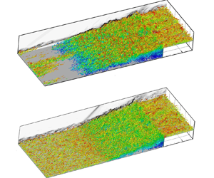
Instantaneous snapshots of vortical structures for the laminar and turbulent cases are illustrated by means of isosurfaces of the  $\lambda _2$ vortex criterion (Jeong & Hussain Reference Jeong and Hussain1995) in figure 8. For the laminar inflow case, distinct turbulent spots emerge in the direct vicinity of the separation line ( $x/h=-25$). At $x/h=-8$, these spots grow rapidly to cover the whole span. The evolution of the coherent vortices, including the formation of the streamwise streaks and the ensuing breakdown, suggests that the boundary layer undergoes a bypass transition, as also reported by Kreilos et al. (Reference Kreilos, Khapko, Schlatter, Duguet, Henningson and Eckhardt2016) and Marxen & Zaki (Reference Marxen and Zaki2019). Entering the region with a stronger recirculation and inflectional velocity profile, the disturbances are amplified significantly, and large hairpin vortices are produced along the shear layer. The multi-scale vortices downstream of the step suggests that the laminar–turbulent transition is completed, which reinforces observations based in the skin friction coefficient in figure 6.

Figure 8. Instantaneous vortical structures, visualized by isosurfaces of  $\lambda _2=-0.12$. A numerical schlieren based on a $z=0$ slice with $|\boldsymbol {\nabla } \rho |/\rho _\infty =0\unicode{x2013}1.4$ is included. The laminar case at $tu_\infty /\delta =900$ is shown (a) upstream of the separation bubble, (b) close to the bubble, and (c) shows the turbulent case at $tu_\infty /\delta =700$.
For the turbulent case, the near-wall region features small-scale vortices in the incoming boundary layer. Since the shear layer over the separation bubble is inviscidly unstable, the vortical structures are enhanced due to strong Kelvin–Helmholtz (K–H) instability. However, a clear signature of spanwise-aligned K–H vortices is not observed because it is overwhelmed by the energetic turbulent structures already present in the incoming shear layer. The amplification of the vortical structures across the separated shear layer was also reported by Mustafa et al. (Reference Mustafa, Parziale, Smith and Marineau2019).
Figure 9 presents the root-mean-square (r.m.s.) fluctuations of the streamwise velocity component,  $\sqrt {\langle u^{\prime 2} \rangle }$ (normalized by $u_\infty$), for the two cases. Large values of $\sqrt {\langle u^{\prime 2} \rangle }$ are observed to occur along the shear layer, between the boundary layer edge and isoline of $\langle u \rangle =0$, for both cases. The laminar case has a peak value of approximately 0.20 in the free shear layer, while the maximum is 0.17 for the turbulent case. While the turbulent case displays weaker fluctuations along the shear layer, larger fluctuations occur along the separation and reattachment shock. Contours of the wall-normal velocity fluctuations $\sqrt {\langle v^{\prime 2} \rangle }$ show similar features (figure 10), but the energetic regions occur closer to the vertical step wall, as reported also by Murugan & Govardhan (Reference Murugan and Govardhan2016). The maximum values of $\sqrt {\langle v^{\prime 2} \rangle }$ are 0.16 near the step wall and 0.12 within the free shear layer for the laminar case; for the turbulent case, the corresponding values are 0.12 near the step and 0.08 in the shear layer. These observations suggest that the shear layer instability is stronger and the separation shock is weaker in the laminar inflow case.

Figure 9. Contours of the time- and spanwise-average standard deviations of the streamwise velocity, normalized by  $u_\infty$: (a) the laminar case, and (b) the turbulent case. The black dashed and solid lines denote isolines of $u=0.0$ and $u/u_e=0.99$.

Figure 10. Contours of the time- and spanwise-average standard deviations of the wall-normal velocity, normalized by  $u_\infty$: (a) the laminar case, and (b) the turbulent case. The black dashed and solid lines denote isolines of $u=0.0$ and $u/u_e=0.99$.
To better visualize the vortical structures near the wall, contours of the streamwise velocity gradient  $\partial u/ \partial y$ in a wall-parallel plane at ${\Delta y/\delta _0=0.01}$ at a random time instant are provided in figure 11. For the laminar case, the velocity gradient is homogeneous far upstream of the step (not shown in the figure) as the incoming boundary layer is laminar. In the separation zone, the contours of $\partial u/ \partial y$ show large streamwise streaks. From the weighted power (spatial) spectral density (PSD) of $\partial u/ \partial y$, we observe a peak at a small spanwise wavenumber $k_z=2$, both upstream and downstream of the step, corresponding to a spanwise wavelength $\lambda _z=0.5h=1.5\delta _0$. For the turbulent case, the contours provide evidence of a streamwise preferential orientation of the near-wall coherent structures upstream of the separation region. Behind the step, streamwise-oriented features are observed again, which suggests large-scale streaks with a spanwise alternation of high and low velocity. Similar to the previous case, the dominant disturbance in the turbulent case also has a spanwise wavenumber at $k_z \approx 2$, yielding again a dominant wavelength $\lambda _z \approx 0.5h \approx 1.5\delta _0$, which is in good agreement with the reported spanwise wavelength of the characteristic vortical structures $\lambda _z \approx 2\delta$ in previous numerical and experimental work (Ginoux Reference Ginoux1971; Pasquariello et al. Reference Pasquariello, Hickel and Adams2017; Priebe & Martín Reference Priebe and Martín2012).

Figure 11. Contours of the streamwise velocity gradient  ${\partial u}/{\partial y}$ in the $x$–
$x$– $z$ plane at the wall distance $\Delta y/\delta _0=0.01$, and the corresponding weighted power spectral density $k_z \mathcal{P}(k_z)$ versus the spanwise wavenumber $k_z$ (black line $x/h=-4.2$; blue line $x/h=1.0$): (a) the laminar case, and (b) the turbulent case.
3.3. Spectral analysis
The frequency characteristics of the interaction are first quantified by the frequency- weighted PSD of selected flow variables. Figure 12 shows the PSD of the wall pressure at different streamwise locations. For this spectral analysis, pressure signals were sampled at frequency  $t_s u_\infty /h=12$ ( $f_s \delta _0 /u_\infty =4$) with $2000$ snapshots, excluding the initial transient stage ( $t u_\infty /\delta _0<600$) of the simulation, which gives a resolved frequency range $0.003 \leq t u_\infty /h \leq 6$. Welch's method with a Hanning window was employed to compute the PSD using eight segments with 50 % overlap. In the following analysis, we use the Strouhal number based on the step height, $St_h=f h/u_\infty$, to characterize the frequency of the unsteady behaviour. Overall, both cases display a broadband frequency spectrum, with different leading frequency at different streamwise locations. For the turbulent inflow case, the spectrum upstream of the recirculation region ( $x/h=-20.0, -16.0$) shows a clear energetic bump centred around the characteristic frequency ( $u_\infty /\delta _0$, corresponding to $St_h=3$) of the incoming turbulent boundary layer (Dolling Reference Dolling2001). For the laminar inflow case, the energy level of the pressure fluctuations is two orders of magnitude lower than that of the turbulent case upstream of the separation region. Within the separation bubble ( $x/h>-11.6$ for the laminar case, $x/h>-4.3$ for the turbulent case), the prevailing frequency shifts to an intermediate range $St_h=0.2\unicode{x2013}1.0$. In addition, a noteworthy low-frequency bump occurs for $St_h < 0.2$ in the separation region, most clearly visible at the station $x/h=-1.0$. Since the laminar inflow case completed transition already inside the separation region and shares similar low-frequency and medium-frequency contents with the turbulent case, mainly the latter case is analysed further hereafter.

Figure 12. Frequency-weighted PSD of the wall pressure at different locations: (a) the laminar case, and (b) the turbulent case. Note that the upstream stations are scaled differently for the laminar inflow case to improve visibility.
As reported in previous work (Pasquariello et al. Reference Pasquariello, Hickel and Adams2017; Hu et al. Reference Hu, Hickel and van Oudheusden2021), the low-frequency unsteadiness is usually associated with the motions of the shock and separation bubble, while the medium-frequency dynamics is related to the shedding of vortices in the separated shear layer. We therefore examine the frequency characteristics of several flow variables to verify if these conclusions apply similarly to the FFS cases. The spanwise-averaged streamwise velocity within the separated shear layer and the reattachment location on the FFS wall both show the dominant medium-frequency unsteadiness. These data are extracted with the same sampling frequency as the aforementioned pressure signal. The location of the spanwise-averaged reattachment point  $y_r$ is the $y$ coordinate of the intersection between the isolines of the streamwise velocity $u=0$ and the step wall. As shown in figure 13(a), a frequency around $St_h=0.3$ appears energetically dominant for the shear layer velocity signal, which supports the suggestion that the medium frequency is the characteristic frequency of the shear layer vortices. In addition, a local peak at a lower frequency $St_h=0.1$ is observed in the spectrum. The shear layer vortices eventually impinge on the step wall, which explains that a similar medium-frequency content is also observed in the spectrum of the reattachment location; see figure 13(b). In addition, there are energetic disturbances with higher frequencies related to the turbulence when the flow reattaches on the wall. It is worth noting that the reattachment point usually moves upwards and downwards at different speeds. To examine this velocity difference at the frequency range, the gradient of the reattachment coordinates ${\rm d}y_r/{\rm d}t$ is calculated with the same sampling frequency $f_s \delta _0 /u_\infty =4$ and then filtered by a low-pass filter with passing frequency $f_p \delta _0 /u_\infty \leq 0.2$. In the given temporal range, the mean value of the positive gradient is 0.0030, and that of the negative gradient is $-0.0032$, which suggest that the reattachment point has a larger speed when moving downwards. Therefore, it takes a shorter time for the attachment point to move downwards, and the probability $P({\rm d}y_r/{\rm d}t<0)$ is smaller (0.46 in total), as shown in figure 14.

Figure 13. Temporal evolution and corresponding frequency-weighted PSD  $f \mathcal{P}(f)$ of (a) the spanwise-averaged streamwise velocity within the shear layer ( $x/h=-3.69$, $y/h=0.83$), and (b) the spanwise-averaged reattachment location.

Figure 14. Probability of the gradient of the reattachment coordinates,  $P({\rm d}y_r/{\rm d}t)$.
Figure 15(a) displays the temporal evolution of the spanwise-averaged separation point  $x_s$, as well as the associated frequency-weighted PSD. The separation point is defined as the streamwise location where appreciable flow reversal is first observed (near-wall streamwise velocity $u/u_\infty < 0.0$). Note that the variation of the mean separation point follows a sawtooth-like trajectory, along which its value drops drastically when the separation point moves upstream while it undergoes a less rapid relaxation when the separation position shifts downstream. The irregular and aperiodic variation of the separation point suggests that the motions of the separation location involve a wide range of time scales, as reported by Dussauge, Dupont & Debiève (Reference Dussauge, Dupont and Debiève2006) and Priebe et al. (Reference Priebe, Tu, Rowley and Martín2016), although the dominant one is the low-frequency one around $St_h \approx 0.1$ shown in the PSD spectra. An additional small peak at a medium frequency $St_h \approx 0.4$ can be observed for the separation point location. It is reasonable to assume that this variable shares common frequencies with the shear layer velocity because the vortex shedding is usually initiated by the separation of the shear layer. Figures 15(b,c) show the temporal variation of the shock angle $\eta$ and separation bubble volume $A$. The shock angle is defined as the angle between the isoline of $y/h=1.0$ and $|\boldsymbol {\nabla } p|\,\delta _0/p_\infty =0.26$. The separation bubble volume is the area enclosed by the isoline of $u=0$, the lower wall and the vertical step wall. Overall, the variation of the shock angle $\eta$ and separation bubble volume $A$ show less irregular features, indicating that the dynamics of these two signals does not involve significant multi-frequency unsteady contents. This is evidenced by the corresponding spectra in figure 15, where we observe very clearly a low-frequency peak at $St_h \approx 0.15$ for the shock angle, and at $St_h \approx 0.08$ for the separation bubble volume.

Figure 15. Temporal evolution and corresponding frequency-weighted PSD of the spanwise-averaged (a) separation location  $x_s$, (b) separation shock angle $\eta$, and (c) volume of the main separation bubble per unit spanwise length $A$.
$A$.
Similar to the reattachment point, these low-frequency signals also have different rates at different states. When the size of the separation bubble increases (the gradient of the bubble volume  ${\rm d}A/{\rm d}t$ is positive), the process of the expansion is slower than the speed of shrinking. In the given temporal range, the mean value of the positive gradient of the bubble volume is 0.0145 and that of the negative gradient is $-0.0167$. Figure 16 shows the probability of various values of ${\rm d}A/{\rm d}t$, indicating that the probability of positive and negative ${\rm d}A/{\rm d}t$ is 0.0041 and 0.0061, respectively. Generally, the separation bubble volume decreases when the reattachment point moves downwards. Therefore, the larger average shrinking rate of the bubble is consistent with the faster downward movement of the reattachment location (see figure 14).

Figure 16. Probability of the changing rate of the separation bubble volume,  $P({\rm d}A/{\rm d}t)$.
To find the connection between the above signals, a statistical analysis was carried out via the coherence  $C_{xy}$ and phase $\theta _{xy}$. The definitions of the spectral coherence and phase are given by
 \begin{gather} C_{xy}(f)=\left| P_{xy}(f) \right|^{2} / \left(P_{xx}(f)\,P_{yy}(f)\right) ,\quad 0 \leq C_{xy} \leq 1, \end{gather}
 \begin{gather} \theta_{xy}(f)=\mathrm{Im}\{P_{xy}(f)\} /\mathrm{Re}\{P_{xy}(f)\} ,\quad {-{\rm \pi}} \leq \theta_{xy} \leq {\rm \pi}, \end{gather}
where  $P_{xx}$ is the PSD of $x(t)$, and $P_{xy}$ signifies the cross-PSD between signals $x(t)$ and $y(t)$.
Figure 17 shows  $C$ and $\theta$ for the relation between the separation location and shock angle. A coherence value $C=0.29$ is observed at $St_h \approx 0.1$, which shows that the separation point and bubble size are nonlinearly related to each other at this specific low frequency. On the other hand, the two signals have a phase difference of roughly $\theta \approx 0.5{\rm \pi}$ at this low frequency. Physically, when the separation location moves downstream (the value of $x_s$ increases), the separation shock foot follows by turning counter-clockwise (the value of $\eta$ increases), and vice versa. The high level of coherence at higher frequency ( $St_h = 0.4$) is caused by the shedding vortices.

Figure 17. Statistical (a) coherence and (b) phase between the spanwise-averaged coordinate of the separation point and the angle of the separation shock.
Figure 18 displays the statistical connection between the separation point and the volume of the separation bubble. We observe significant coherence at frequencies  $St_h < 0.1$, accompanied with phase $\theta \approx -{\rm \pi}$. That is, the bubble size increases when the separation point moves upstream at low frequencies. The phase difference, however, changes at higher frequencies $St_h \approx 0.15$, where $\theta \approx 0.25{\rm \pi}$. These results confirm previous observations that there is no simple linear relation between separation length and bubble volume (Adler & Gaitonde Reference Adler and Gaitonde2018).

Figure 18. Statistical (a) coherence and (b) phase between the spanwise-averaged streamwise coordinate of the separation point and the volume of the separation bubble.
For the signals of the reattachment location and the bubble size in figure 19, significant correlation can be found for a broad range of frequencies ( $St_h > 0.1$). The near-zero $\theta$ implies that these two signals are approximately in phase for the low-frequency range, meaning that an upwards motion of the reattachment point is accompanied by an increase of the bubble size. At frequencies $St_h > 0.1$, the separation bubble will expand (increasing $A$) if the separation point moves downstream (increasing $x_s$) and the reattachment location moves upwards (increasing $y_r$). In this dilatation process of the bubble, the separation length reduces, while the separation height becomes larger, which suggests that the volume of the separation bubble depends mainly on the separation height (the reattachment location in the current case) at $St_h > 0.1$, whereas the separation length is in phase with the bubble size at lower frequency frequencies $St_h < 0.1$.

Figure 19. Statistical (a) coherence and (b) phase between the spanwise-averaged wall-normal coordinate of the reattachment point and the volume of the separation bubble.
3.4. Dynamic mode decomposition analysis of the three-dimensional flow field
We have applied DMD (Schmid Reference Schmid2010) to identify the modal dynamics and energetic flow structures contributing to the broadband frequency spectrum. In § 3.3, we identified two types of dominant frequencies in the unsteady interaction system. However, some of the signals were extracted from the spanwise-averaged field, like the separation and reattachment locations; therefore a three-dimensional DMD analysis is required for the analysis of possible effects of spanwise variant flow structures. A spatial subdomain is extracted from the simulated flow domain for the three-dimensional DMD analysis in order to reduce the computational effort. The considered subdomain is  $L_x \times L_y \times L_z=([-25,15]\times [0,8]\times [-8,8])\delta _0$, covering the most interesting region, with a downsampled spatial resolution in all directions. Since the frequencies above the characteristic frequency of the turbulent integral scale $u_\infty / \delta _0$ are not our current interest, the present DMD analysis of the three-dimensional subdomain is performed based on $1000$ equal-interval snapshots with the same time range as for the previous signals and a smaller sampling frequency $f_s \delta _0/u_\infty =2$, which yields a frequency resolution $2\times 10^{-3} \leq f \delta _0/u_\infty \leq 1$ (equivalent to $6\times 10^{-3} \leq St_h \leq 3$). The calculated eigenvalue spectrum and magnitudes of the corresponding DMD modes are displayed in figure 20. The resulting DMD modes come as complex conjugate pairs, and most of them are well distributed along the unit circle $|\mu _k|=1$ except for a few decaying modes within the circle, which means that the resulting modes are sufficiently saturated (Rowley et al. Reference Rowley, Mezić, Bagheri, Schlatter and Henningson2009). In figure 20(b), the shown modes are grey shaded by their growth rate $\beta _k$. The darker the vertical lines, the less decaying the modes. Here, the strongly decaying modes ( $|\mu _k|\leq 0.96$) have been removed because they do not contribute to the long-time flow development.

Figure 20. (a) Eigenvalue spectrum from the standard DMD. (b) Normalized magnitudes for DMD modes with positive frequency, grey shaded by their growth rate  $\beta _k$.
From the previous spectral analysis, two types of frequencies have been identified. These frequencies are also significant in figure 20(b). Therefore, two corresponding families of modes are defined in the spectrum, a low-frequency family at  $St_h<0.2$ (family A) and a medium-frequency family at $0.2 \leq St_h \leq 1.0$ (family B), and the different features characteristic for each family are investigated. In addition, an extra family of modes at $St_h>1.0$ (family C, close to the characteristic frequency of the turbulent integral scale) is also analysed. Based on the growth rate and magnitudes of the modes, three modes are selected from the frequency spectrum, each of which is a representative of a single family, marked as mode $\phi _1$, $\phi _2$ and $\phi _3$, respectively. Table 4 gives the non-dimensional frequency, magnitude and growth rate of these selected modes. All of them have relatively large magnitude with $|\psi _k|>0.4$, and small growth rate with $|\beta _k|<0.02$, which indicates that they have a relevant contribution to the evolution of the flow field over the full analysed time span.
Table 4. Information for the selected modes.

The selected mode  $\phi _1$ has frequency $St_h=0.0377$, which has the same order of magnitude as the data ( $St_h=0.017$) reported by Estruch-Samper & Chandola (Reference Estruch-Samper and Chandola2018). Figure 21 shows the pressure fluctuations from mode $\phi _1$ at two different phase angles. The main features of the pressure fluctuations are large structures along the separation shock and the reattachment shock. The sign switch between the two displayed phase angles indicates the oscillation of the shock. Note that the fluctuations around the separation and reattachment shocks are also moving in the spanwise direction, suggesting a slight wrinkling of the shocks. Figure 22(a) provides the pressure fluctuations of $\phi _1$ at the slice $z=0$. Again, large fluctuations are observed around the separation and reattachment shocks. There are also waves induced by the separation shock propagating along the streamwise direction.

Figure 21. Isosurfaces of the pressure fluctuations from DMD mode  $\phi _1$ with phase angle (a) $\theta =0$ and (b) $\theta =3{\rm \pi} /4$, including only the real part. Red indicates $p^{\prime }/p_\infty =0.03$; blue indicates $p^{\prime }/p_\infty =-0.03$.

Figure 22. Real part of DMD mode  $\phi _1$ indicating contours of modal (a) pressure fluctuations and (b) streamwise velocity fluctuations, on the slice $z=0$. The different lines indicate features of the mean flow field: green solid line, the separation shock; black dashed line, dividing streamline; green dashed line, the streamline passing through $x/\delta _0=0$, $y/\delta _0=3.75$.
The fluctuations of the streamwise velocity component from DMD mode  $\phi _1$ are given in figure 23. From the isosurfaces of $u^{\prime }/u_\infty =\pm 0.2$, we observe pairs of longitudinal streamwise structures, which emerge around the separation location and extend into the free shear layer and towards the downstream boundary layer. Considering the contours of the streamwise velocity fluctuations on the $z=0$ slice in figure 22(b), we find that these high- and low-speed structures are located mainly along the shear layer.

Figure 23. Isosurfaces of the streamwise velocity fluctuations from DMD mode  $\phi _1$ with phase angle (a) $\theta =0$ and (b) $\theta =3{\rm \pi} /4$, including only the real part. Red indicates $u^{\prime }/u_\infty =0.2$; blue indicates $u^{\prime }/u_\infty =-0.2$.
The streaks visualized by the isosurfaces of the streamwise velocity fluctuation are a possible result of momentum transport by counter-rotating streamwise vortices. Therefore, we plot the contours of the modal streamwise vorticity and projected streamlines at two phase angles, as shown in figure 24. The counter-rotating vortices are illustrated clearly by the in-plane streamlines. Additionally, these vortices move in both the spanwise and wall-normal directions, and their strength is also changing with the phase angle. At the given instants ( $\theta =3{\rm \pi} /16$ and $\theta =7{\rm \pi} /16$), the spanwise wavelength of the vortex pair is ranging from $0.5h$ to $0.6h$. Based on these observations, we believe that the dynamics represented by the low-frequency mode $\phi _1$ involves the flapping motions of the separation and reattachment shock, as well as oscillating Görtler-like vortices in the shear layer.

Figure 24. Contours of the streamwise vorticity from DMD mode  $\phi _1$ with phase angle (a) $\theta =3{\rm \pi} /16$ and (b) $\theta =7{\rm \pi} /16$, in the $z$–
$z$– $y$ plane at $x/\delta _0=-6.0$. Black arrow lines represent the streamlines on the slice.
To better illustrate the flow dynamics corresponding to a selected DMD mode, we reconstructed the real-valued flow field by superimposing the individual mode  $\phi _i$ onto the mean flow $\phi _m$, expressed as $q(x,t)=\phi _m + a_f \times \mathrm {Re} \{\alpha _i \phi _i\,{\rm e}^{{\rm i}\omega _i t}\}$, where $\alpha _i$ and $a_f$ are the amplitude and optional amplification factor of the considered mode $\phi _i$. Animations of the dynamic flow field reconstructed with a single mode using this procedure are provided as supplementary movies available at https://doi.org/10.1017/jfm.2022.737. Movies 1 and 2 (reconstructed from mode $\phi _1$) show clearly the flapping motion of the separation shock and the counter-rotating Görtler vortices. Other modes from the low-frequency branch A were found to share very similar flow features with the selected mode $\phi _1$.
For the medium-frequency mode  $\phi _2$, the characteristic frequency is $St_h \approx 0.349$, which is in good agreement with the experimental results ( $St_h \approx 0.4$) of Estruch-Samper & Chandola (Reference Estruch-Samper and Chandola2018). The pressure isosurfaces in figure 25 exhibit large spanwise-aligned structures arranged along the free shear layer. These significant fluctuations represent the travelling shear layer vortices. In the contours of the modal spanwise-averaged pressure fluctuations in figure 26, the radiation of the waves along the shear layer is obvious. The emission of these structures induces disturbances along the streamwise direction in the supersonic part of the flow field. This observation of the propagating pressure waves is in agreement with the results from a global linear stability analysis of an impinging shock case in a laminar regime (Guiho, Alizard & Robinet Reference Guiho, Alizard and Robinet2016).

Figure 25. Isosurfaces of the pressure fluctuations from DMD mode  $\phi _2$ with phase angle (a) $\theta =0$ and (b) $\theta =3{\rm \pi} /4$, including only the real part. Red indicates $p^{\prime }/p_\infty =0.03$; blue indicates $p^{\prime }/p_\infty =-0.03$.

Figure 26. Real part of DMD mode  $\phi _2$ indicating contours of modal spanwise-averaged (a) pressure fluctuations and (b) streamwise velocity fluctuations, on the slice $z=0$. The different lines indicate features of the mean flow field: green solid line, the separation shock; black dashed line, dividing streamline; green dashed line, the streamline passing through $x/\delta _0=0$, $y/\delta _0=3.75$.
Figure 27 shows isosurfaces of the streamwise velocity fluctuations associated with mode  $\phi _2$. Here, $\varLambda$-shaped structures are observed in the free shear layer and alternate along both the spanwise and streamwise directions. Supplementary movies 3 and 4 (reconstructed from mode $\phi _2$) visualize the convection of shear layer vortices and the propagation of the Mach-like waves. These observations confirm that this mode, which is representative of the mid-frequency dynamics, is indeed related to the advection of the shear layer vortices. Similar observations were also reported in the two-dimensional DMD analysis of an incident shock case (Pasquariello et al. Reference Pasquariello, Hickel and Adams2017).

Figure 27. Isosurfaces of the streamwise velocity fluctuations from DMD mode  $\phi _2$ with phase angle (a) $\theta =0$ and (b) $\theta =3{\rm \pi} /4$, including only the real part. Red indicates $u^{\prime }/u_\infty =0.2$; blue indicates $u^{\prime }/u_\infty =-0.2$.
Considering the high-frequency mode  $\phi _3$, the pressure fluctuations provided in figure 28 show the evolution of small-scale vortices. These spanwise-aligned vortices are weakly visible also in the upstream turbulent boundary layer and amplified in the free shear layer. The streamwise displacement of the fluctuations at different phase angles indicates the advection of these coherent vortices. From the streamwise velocity fluctuations of mode $\phi _3$ in figure 29, we can also observe that these vortices originate from the upstream turbulence and are considerably amplified in the separated shear layer. The frequency of this mode is close to the typical frequency of the turbulence considering the thicker boundary layer downstream of the step. Hence this mode can be associated with the advection of turbulent structures that results from an amplification of the incoming turbulence by the separation bubble; cf. the stability analysis of Guiho et al. (Reference Guiho, Alizard and Robinet2016) for an incident shock SWBLI case.

Figure 28. Isosurfaces of the pressure fluctuations from DMD mode  $\phi _3$ with phase angle (a) $\theta =0$ and (b) $\theta =3{\rm \pi} /4$, including only the real part. Red indicates $p^{\prime }/p_\infty =0.06$; blue indicates $p^{\prime }/p_\infty =-0.06$.

Figure 29. Isosurfaces of the streamwise velocity fluctuations from DMD mode  $\phi _3$ with phase angle (a) ${\theta =0}$ and (b) $\theta =3{\rm \pi} /4$, at slice $z=0$, including only the real part. Red indicates $u^{\prime }/u_\infty =0.4$; blue indicates $u^{\prime }/u_\infty =-0.4$.
4. Physical mechanism of the low-frequency unsteadiness
The present FFS case exhibits unsteady dynamics at non-dimensional low frequencies similar to those observed for SWBLI on flat plates, compression ramps and BFS. Similar to the compression ramp (Grilli et al. Reference Grilli, Hickel and Adams2013), the main flow topology of the FFS case consists of a separation shock, free shear layer, separation bubble and reattachment shock (not as prominent as for the compression ramp). Therefore, the streamwise profiles of the mean skin friction and wall pressure have very similar trends for FFS and ramp cases (Priebe et al. Reference Priebe, Tu, Rowley and Martín2016). However, differences of  $\langle C_f \rangle$ and $\langle p_w \rangle$ curves are observed due to the confinement by the step wall. As we can see in figures 6 and 7, there is a drastic rise of $\langle C_f \rangle$ and a smaller second plateau of $\langle p_w \rangle$ around the step, which are not observed for the ramp and incident shock cases (Priebe & Martín Reference Priebe and Martín2012). The variations of these parameters inside the separation bubble are usually related to the multi-frequency unsteadiness (Priebe et al. Reference Priebe, Tu, Rowley and Martín2016; Pasquariello et al. Reference Pasquariello, Hickel and Adams2017).
The instantaneous flow field shown in § 3.2 visualizes the main unsteady phenomena, including the breathing bubble, oscillation of the separation and reattachment shocks, the shear layer, and the high- and low-speed streaks, which also occur in ramp, impinging shock and BFS configurations. As characterized by the DMD analysis of the three-dimensional flow field, the low-frequency DMD modes include unsteady shock motions and counter-rotating streamwise vortices. These Görtler-like vortices are relatively weak compared to other unsteady dynamics such that they do not show up in the vortical visualization of the complete flow field (see figure 8). The medium-frequency modes, on the other hand, are associated with the shedding of vortices within the shear layer. Similar observations have been reported in the impinging shock and ramp shock interaction configurations, as well as in our previous work related to the BFS (Hu et al. Reference Hu, Hickel and van Oudheusden2021).
Piponniau et al. (Reference Piponniau, Dussauge, Debiève and Dupont2009) found that the separation bubble is highly intermittent based on their conditional average of the bubble size, and proposed an entrainment-injection model to explain the dynamics of the low-frequency unsteadiness. This model associates the low-frequency motion of the shear layer with an unbalanced mass budget within the separation bubble. In the current FFS case, we also observe a strong intermittency of the bubble size with large-scale variations in magnitude (see figure 15) for the expanding and contracting phase, as illustrated schematically in figure 31. In the contraction process, the fluid from the separation region is entrained by the coherent structures along the mixing layer in the initial phase of the separation. After a certain distance, these vortices are shed from the shear layer and enter the downstream outer flow carrying mass with themselves, which causes a mass deficit of the separation bubble. The separated region shrinks with a downward motion of the reattachment location and an upstream shift of the separation point. Accordingly, the foot of the separation shock moves upstream. The continuous loss of the mass inside the bubble, however, cannot be maintained. There must be a reverse mass transfer such that the separation bubble will expand.
To ensure a continuous breathing of the separated region, the mass of the injection should be equal to the total amount of mass discharging through the shear layer. We also expect that it takes several periods of the shedding vortices before they drain out a considerable amount of fluid mass. Therefore, it is reasonable to assume that the frequency of the breathing motions is smaller than that of the shedding behaviour, which agrees with the findings in §§ 3.3 and 3.4. Based on the above reasoning, we believe that the entrainment-injection model is also applicable for the FFS configuration.
However, there must be a mechanism to support the large-scale motions of the interaction region. The current DMD suggests that the spanwise oscillation of counter-rotating Görtler-like vortices may be the driver behind the low-frequency unsteadiness, as we proposed in the previous BFS case (Hu et al. Reference Hu, Hickel and van Oudheusden2021). The Görtler number defined as
 \begin{equation} G_t=\frac{\theta^{3/2}}{0.18\delta^{*}\,|R|^{1/2}} , \end{equation}
indicates whether such vortices can form (Smits & Dussauge Reference Smits and Dussauge2006), where  $R$ is the radius of curvature of the streamline, $\delta ^{*}$ is the boundary layer displacement thickness, and $\theta$ is the boundary layer momentum thickness. Figure 30 shows the curvature $h/R$ and Görtler number $G_t$ along the streamline of the mean flow inside the shear layer (shown in figure 22). As we can see, two distinct peaks are observed in the distribution of the curvature, located around the separation and reattachment points. This strong curvature induces strong Görtler instability, corresponding to the high levels of $G_t$ around the separation and reattachment locations. At $-6.5\leq x/h \leq -3.3$ and $0\leq x/h \leq 1$, the Görtler number is larger than the critical value $G_t=0.6$, above which local Görtler vortices will emerge in a laminar flow (Smits & Dussauge Reference Smits and Dussauge2006). Therefore, we believe that the Görtler instability is the cause of the Görtler-like vortices, visualized by the streamwise velocity fluctuations (figure 23) and streamlines (figure 24) from DMD mode $\phi _1$.

Figure 30. (a) Curvature  $h/R$ and (b) Görtler number $G_t$, along the mean streamline passing through $x/h=0$ and $y/h=1.25$ (for the fully turbulent case). Vertical dashed lines indicate the separation and reattachment points. The horizontal dot-dashed line denotes the critical $G_t$ in a laminar flow.
The separation location on any given slice  $z=z_1$ moves as a result of the spanwise translation of Görtler vortices, as illustrated by figure 31. In the contraction process (from $t_1$ to $t_2$), when the counter-rotating Görtler-like vortices move towards the positive spanwise direction, the streamwise velocity $u$ will become negative from $u=0$ at the ${z=z_1}$ location (see the schematic in figure 31a), which means that the flow direction reverses from $t_1$ to $t_2$ at this specific location. The upstream movement of the separation point leads to the upstream flapping of the separation shock. Correspondingly, the reattachment point shifts downwards, and mass is entrained by the shear layer. The consecutive oscillations of the interaction region result in a wrinkling of the shock and the breathing of the bubble. Oppositely, if the Görtler-like vortices move towards the negative spanwise direction from $t_1$ to $t_2$ (see the schematic in figure 31b), then the separation point will (at $t=t_1$) become a part of the attached flow (at $t=t_2$) at slice $z=z_1$, and the separation shock will move downstream.

Figure 31. Sketch of the entrainment-injection model sustained by the Görtler vortices: (a) contraction process and (b) dilatation process.
In terms of the magnitude of the low frequencies, the current results for an FFS yield a Strouhal number range  $0.02< St_h<0.2$ , close to the frequencies obtained in other canonical incident shock and ramp cases ( $0.01< St_h<0.2$, normalized by the height of the separation bubble). Based on the above analysis, we believe that the entrainment-injection model can explain the low-frequency unsteadiness of SWBLI.
5. Conclusions
The low-frequency unsteady dynamics of the SWBLI over an FFS at  $Ma=1.7$ and $Re_{\delta _0}=13\,718$ has been analysed based on well-resolved LES. The instantaneous vortical visualizations indicate that the unsteady behaviour is similar to what we observe in the BFS case, including the vortex shedding in the separated shear layer, the breathing of the separation bubble, and the flapping motion of the main shock. From the spectral analysis, we observe that there is a broadband low/medium-frequency dynamics in the interaction region, which we classify into two branches with dominant frequencies at $St_h=0.01\unicode{x2013}0.2$ and $St_h=0.2\unicode{x2013}1.0$ in the current FFS case. The medium-frequency content is associated with the shedding of shear layer vortices, while the unsteady separation region – more specifically, the size of the separated region – and the position and angle of the separation shock constitute the low-frequency dynamics.
Three-dimensional DMD analysis was applied to identify individual single-frequency modes that represent the observed unsteady behaviour. Similar to what we observed in the BFS case (Hu, Hickel & van Oudheusden Reference Hu, Hickel and van Oudheusden2020), the extracted low-frequency mode  $\phi _1$ suggests that there is a statistical link between the shock motions and unsteady Görtler-like vortices. The flow features displayed by the medium-frequency mode $\phi _2$ represent the advection of shear layer vortices.
Based on the above observations and analysis, we consider that the physical mechanism of the low-frequency unsteadiness in the FFS is very similar to the one for other canonical SWBLI cases. We believe that the unsteady Görtler-like vortices impose an unsteady forcing on the interaction system that sustains the low-frequency motions of shocks and separation bubble.
Supplementary movies
Supplementary movies are available at https://doi.org/10.1017/jfm.2022.737.
Acknowledgements
The authors would like to thank J. Chen and X. Yuan for fruitful discussions at the State Key Laboratory of Aerodynamics, which helped to improve the paper.
Funding
This work is part of the research programme ‘Dynamics of a Backward/Forward-Facing Step in a Supersonic Flow’ with project no. 2019.045, which is partly financed by the Dutch Research Council (NWO). The simulations were carried out on the Dutch national e-infrastructure with the support of SURF Cooperative.
Declaration of interests
The authors report no conflict of interest.


 Open access