


1. Introduction
Large eddy simulation (LES) is becoming an increasingly important technique for the accurate prediction of turbulence and is regarded as one of the key techniques for computational fluid dynamics in the coming years (e.g. NASA CFD Vision 2030 by Slotnick et al. (Reference Slotnick, Khodadoust, Alonso, Darmofal, Gropp, Lurie and Mavriplis2014)). In LES, the energy-containing eddies are resolved by the computational grid, while the effects of the smaller eddies which are not resolved by the grid are modelled using a subgrid scale (SGS) model. While this methodology reduces the number of grid points required, LES is still computationally expensive for use in industrial applications, especially when applied to wall-bounded flows. For example, Tamaki & Kawai (Reference Tamaki and Kawai2023) performed an LES of the flow around an airfoil at a chord-based Reynolds number of $Re_c = 10^7$
using the state-of-the-art supercomputer Fugaku. This simulation required approximately
$Re_c = 10^7$
using the state-of-the-art supercomputer Fugaku. This simulation required approximately $38 \times 10^9$
grid points to resolve the dynamically important near-wall turbulent eddies which become progressively small with increasing Reynolds number. Such high-Reynolds-number flow simulations, while crucial for computer-aided engineering, are only possible using top-performing supercomputers. For industries to apply LES in their early design stages, the computational cost of the LES is desired to be made more affordable. In this study, we consider using coarser computational grids than the conventional well-resolved LES to reduce the number of grid points. In particular, we target cases where even the energetic eddies are not sufficiently resolved.
$38 \times 10^9$
grid points to resolve the dynamically important near-wall turbulent eddies which become progressively small with increasing Reynolds number. Such high-Reynolds-number flow simulations, while crucial for computer-aided engineering, are only possible using top-performing supercomputers. For industries to apply LES in their early design stages, the computational cost of the LES is desired to be made more affordable. In this study, we consider using coarser computational grids than the conventional well-resolved LES to reduce the number of grid points. In particular, we target cases where even the energetic eddies are not sufficiently resolved.
With coarse computational grids, a larger fraction of the turbulent kinetic energy must be modelled by the SGS model. An example for SGS modelling is the eddy-viscosity style model, such as the Smagorinsky model (Smagorinsky Reference Smagorinsky1963; Lilly Reference Lilly1966), the dynamic Smagorinsky model (Germano et al. Reference Germano, Piomelli, Moin and Cabot1991) and selective mixed-scale model (Lenormand et al. Reference Lenormand, Sagaut, Phuoc and Comte2000). However, while they accurately model the average dissipation of kinetic energy for typical well-resolved LES, they are known to perform poorly for wall turbulence with coarse grids (Jimenez & Moser Reference Jimenez and Moser2000). It is shown that the eddy-viscosity approximation is unable to accurately predict the mean SGS stresses, which becomes increasingly important for wall turbulence with coarse grids. This error occurs because the eddy-viscosity approach expresses the SGS stresses as scalar multiples of the velocity gradient tensor, which does not hold well in real turbulence. Another approach, the scale similarity model (Bardina, Ferziger & Reynolds Reference Bardina, Ferziger and Reynolds1980), is able to more accurately reproduce the exact SGS stress components. However, this approach is shown to poorly predict the energy dissipation. Combining the eddy-viscosity and scale similarity ideas, Abe (Reference Abe2013) showed that splitting the SGS stress tensor into dissipative and non-dissipative components and modelling them separately significantly improves the prediction of wall turbulence with coarse grids. Close analyses of this SGS-modelling approach revealed that the newly included terms significantly contribute to the redistribution of velocity fluctuations among the three directions, which are confirmed by direct numerical simulation (DNS) data to be indispensable to the regeneration of turbulence (Inagaki & Kobayashi Reference Inagaki and Kobayashi2022, Reference Inagaki and Kobayashi2023).
In these SGS models, the SGS stress components are calculated from the resolved grid-scale quantities with the assumption that the resolved quantities are physically accurate. With very coarse grids focused on in this study, however, even the energy-containing turbulent structures are intended not to be sufficiently resolved, which results in the non-physical turbulent structures and statistics (which will be shown later). In this regard, the non-physical turbulence in the resolved scales prevent conventional SGS models from accurate predictions of SGS components, resulting in inaccurate turbulent statistics (Rezaeiravesh & Liefvendahl Reference Rezaeiravesh and Liefvendahl2018).
Machine learning is known to successfully find relationships among data that are difficult to identify, and has also been applied to fluid mechanics (cf. the review by Brunton, Noack & Koumoutsakos (Reference Brunton, Noack and Koumoutsakos2020)). Some studies have applied machine learning to SGS modelling (Gamahara & Hattori Reference Gamahara and Hattori2017; Lapeyre et al. Reference Lapeyre, Misdariis, Cazard, Veynante and Poinsot2019; Subel et al. Reference Subel, Chattopadhyay, Guan and Hassanzadeh2021). In particular, based on machine-learning-based turbulence super-resolution, Bode et al. (Reference Bode, Gauding, Lian, Denker, Davidovic, Kleinheinz, Jitsev and Pitsch2021) modelled the SGS stresses as the difference between the filtered DNS data and the reconstructed DNS flow field.
Most studies in the field of machine-learning-based turbulence super-resolution are based on supervised machine learning (e.g. Fukami, Fukagata & Taira (Reference Fukami, Fukagata and Taira2019), Deng et al. (Reference Deng, He, Liu and Kim2019) and Liu et al. (Reference Liu, Tang, Huang and Lu2020); also see review by Fukami, Fukagata & Taira (Reference Fukami, Fukagata and Taira2023)), in which the input and its expected output are given in pairs as the training data. For the training of SGS models, filtered DNS (fDNS) data are usually used as the input, and the original DNS flow field is used as the output to extract the SGS stress components. Generally, machine learning models make accurate super-resolution predictions within the statistical distributions of their training data. In this regard, the typical training method assumes that fDNS data and LES data have similar turbulent statistics, i.e. fDNS $\approx$
LES. However, as mentioned above, very coarse-grid LES (vLES) flow fields have different statistics from fDNS, i.e. fDNS
$\approx$
LES. However, as mentioned above, very coarse-grid LES (vLES) flow fields have different statistics from fDNS, i.e. fDNS $\neq$
vLES. In this case, typical SGS models based on the supervised machine learning trained on fDNS data are expected to be inappropriate for vLES. A similar problem is also discussed in a review paper by Duraisamy (Reference Duraisamy2021).
$\neq$
vLES. In this case, typical SGS models based on the supervised machine learning trained on fDNS data are expected to be inappropriate for vLES. A similar problem is also discussed in a review paper by Duraisamy (Reference Duraisamy2021).
The above argument requires that the machine learning model be trained using vLES and DNS data. An issue with this approach is that because the LES and DNS flow fields are obtained separately, it is not possible to obtain the corresponding pairs of instantaneous DNS and LES data that are required for supervised machine learning. In the case of well-resolved LES, this problem can be overcome by using the fDNS data as a substitute for the LES data since fDNS $\approx$
LES. On the other hand, because vLES and fDNS data are significantly different (fDNS
$\approx$
LES. On the other hand, because vLES and fDNS data are significantly different (fDNS $\neq$
vLES) as considered in this study, fDNS data cannot be used as the substitute. Therefore, it is necessary to use an unsupervised machine-learning architecture to train this machine learning model.
$\neq$
vLES) as considered in this study, fDNS data cannot be used as the substitute. Therefore, it is necessary to use an unsupervised machine-learning architecture to train this machine learning model.
In the field of image transformation, Zhu et al. (Reference Zhu, Park, Isola and Efros2020) have proposed the cycle-consistency generative adversarial network (GAN) (CycleGAN). The CycleGAN enables one type of image to be transformed into another type of image without the need for paired training data. For example, CycleGAN can be used to transform an image of a horse into that of a zebra, without requiring a picture of a zebra at the same location as the horse. This relationship between images of horses and zebras is similar to that of LES and fDNS. In fact, Kim et al. (Reference Kim, Kim, Won and Lee2021) showed that CycleGAN can be used to perform super-resolution of wall-parallel slices from a conventional well-resolved LES of turbulent channel flow. In this study, we employ the CycleGAN to construct a machine-learning-based SGS model that enable accurate predictions on coarse computational grids. Specifically, we employ CycleGAN to convert the erroneous vLES flow fields to be physically accurate LES flow fields (i.e. fDNS-quality flow fields). Then, typical supervised methods may be used to accurately super-resolve the fDNS-quality flow fields and extract the SGS stresses.
In this study, we propose an unsupervised and supervised machine learning pipeline for SGS modelling of vLES utilising CycleGAN as its unsupervised part. The proposed machine learning pipeline performs super-resolution of vLES flow fields to output DNS-quality flow fields. The predicted high-wavenumber components in the DNS-quality flow fields are then extracted as SGS stress components. The proposed method is tested in a turbulent channel flow in both a priori and a posteriori tests at the friction Reynolds number of $Re_\tau \approx 1000$
. For the a posteriori test, the method is also tested at a higher Reynolds number
$Re_\tau \approx 1000$
. For the a posteriori test, the method is also tested at a higher Reynolds number $Re_\tau \approx 2000$
which is outside of the training dataset.
$Re_\tau \approx 2000$
which is outside of the training dataset.
We emphasise that a key distinguishing factor of the proposed unsupervised and supervised machine learning pipeline is that it operates on the non-physical flow fields of vLES to physically consistent flow fields for SGS modelling. While previous research on supervised super-resolution achieves super-resolution from extremely coarse input data (e.g. up to 32-times coarser data (Fukami et al. Reference Fukami, Fukagata and Taira2019; Yousif, Yu & Lim Reference Yousif, Yu and Lim2021)), such input data are typically taken from physically accurate fDNS and therefore assumed to be physically accurate coarse data. Therefore, well-established and widely used supervised methods have not been shown to be effective for the non-physical flow fields of vLES. Additionally, the unsupervised super-resolution method demonstrated by Kim et al. (Reference Kim, Kim, Won and Lee2021) was only verified for well-resolved LES (four-times courser than DNS), and thus the input data do not contain non-physical flow structures. This study explores in detail the effectiveness of the proposed unsupervised–supervised method for super-resolution and SGS modelling in both a priori and a posteriori manners.
We note that, as mentioned above, the coarse computational grid that is the target of this study cannot fully resolve the most energetic eddies of turbulence. Therefore, in this paper, our primary purpose is the accurate prediction of the mean streamwise velocity (first-order statistics). Correspondingly, the shear stress balance in the boundary layer requires the accurate prediction of the Reynolds shear stress. On the other hand, accurate predictions of the Reynolds normal stresses and the higher-order statistics are not the primary purpose of this study. However, the high-order statistics will also be investigated in this paper to elucidate their effects on the prediction of the mean velocity and Reynolds shear stress.
This paper is structured as follows. In § 2, the theoretical basis of the LES and the employed machine learning techniques are reviewed. In § 3, the architecture of our proposed pipeline is discussed. The details of the tests performed on the proposed pipeline are given in § 4. We validate that the proposed unsupervised and supervised machine learning pipeline enables appropriate super-resolution and prediction of SGS stresses in an a priori test in § 5. Section 6 tests the performance of the proposed SGS modelling methodology in the LES using a very coarse grid and investigate the turbulence mechanism that yields the change in the predicted statistics. The robustness of the proposed methodology to a different Reynolds number from the training data are discussed in § 7. We conclude our study in § 8.
2. Governing equations and machine learning
2.1. Large-eddy simulation
Large-eddy simulation is a method for turbulence simulation in which the large energy-containing eddies are resolved by the computational grid, while the effects of the small eddies are modelled using SGS models. The compressible LES is used in this study, and the compressible Navier–Stokes equations are
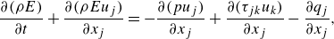
 \begin{align}&\qquad\qquad\qquad\,\, \frac {\partial \rho }{\partial t} + \frac {\partial (\rho u_j)}{\partial x_j} =0,\\[-10pt]\nonumber \end{align}
 \begin{align}&\qquad \frac {\partial (\rho u_i)}{\partial t} + \frac {\partial (\rho u_i u_j )}{\partial x_j} = - \frac {\partial (p \delta _{ij})}{\partial x_j} + \frac {\partial \tau _{ij}}{\partial x_j},\\[-10pt]\nonumber \end{align}
 \begin{align}& \frac {\partial (\rho E)}{\partial t} + \frac {\partial (\rho E u_j)}{\partial x_j} = - \frac {\partial (p u_j)}{\partial x_j} + \frac {\partial (\tau _{jk} u_k)}{\partial x_j} - \frac {\partial q_j}{\partial x_j}, \end{align}
where $\rho , u, p$
denote the density, velocity and pressure, respectively. Here
$\rho , u, p$
denote the density, velocity and pressure, respectively. Here $E$
is the total energy defined as
$E$
is the total energy defined as
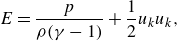 \begin{equation} E = \frac {p}{\rho (\gamma - 1)} + \frac {1}{2} u_k u_k, \end{equation}
with the heat capacity ratio of $\gamma = 1.4$
(ideal gas). Here
$\gamma = 1.4$
(ideal gas). Here $\tau _{ij}$
are the components of the viscous stress tensor defined as
$\tau _{ij}$
are the components of the viscous stress tensor defined as
 \begin{align}&\qquad\quad \tau _{ij} = \mu (T) S_{ij},\\[-10pt]\nonumber \end{align}
 \begin{align}& S_{ij} = \frac {\partial u_i}{\partial x_j}+\frac {\partial u_j}{\partial x_i} - \frac {2}{3} \delta _{ij} \frac {\partial u_k}{\partial x_k}, \end{align}
where $\mu (T)$
denotes the molecular viscosity calculated as a function of the temperature
$\mu (T)$
denotes the molecular viscosity calculated as a function of the temperature $T$
by Sutherland’s law. Here
$T$
by Sutherland’s law. Here $q_i$
is the heat flux vector defined as
$q_i$
is the heat flux vector defined as
 \begin{equation} q_i = - \kappa (T) \frac {\partial T}{\partial x_i}, \end{equation}
where $\kappa (T)$
is the heat conductivity as a function of the temperature.
$\kappa (T)$
is the heat conductivity as a function of the temperature.
An arbitrary quantity $f$
can be decomposed into its spatially filtered value
$f$
can be decomposed into its spatially filtered value $\overline {f}$
and deviations
$\overline {f}$
and deviations $f^{\prime}$
as
$f^{\prime}$
as $f = \overline {f} + f^{\prime}$
. Applying the filtering operation
$f = \overline {f} + f^{\prime}$
. Applying the filtering operation $\overline {(\cdot )}$
to (2.1)–(2.3) and neglecting the insignificantly small terms yields the following spatially filtered Navier–Stokes equations (i.e. the LES equations) (Vreman Reference Vreman1995):
$\overline {(\cdot )}$
to (2.1)–(2.3) and neglecting the insignificantly small terms yields the following spatially filtered Navier–Stokes equations (i.e. the LES equations) (Vreman Reference Vreman1995):
 \begin{align}&\qquad\qquad\qquad\qquad\qquad\qquad \frac {\partial \overline {\rho }}{\partial t} + \frac {\partial (\overline {\rho } \widetilde {u_j})}{\partial x_j} = 0, \end{align}
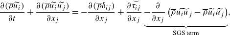 \begin{align}&\qquad \frac {\partial (\overline {\rho }\widetilde {u_i})}{\partial t}+ \frac {\partial (\overline {\rho }\widetilde {u_i}\widetilde {u_j})}{\partial x_j} = - \frac {\partial (\overline {p}\delta _{ij})}{\partial x_j} + \frac {\partial \overset {\smile }{\tau _{ij}}}{\partial x_j} \underbrace { - \frac {\partial }{\partial x_j} \left ( \overline {\rho } \widetilde {u_i u_j} - \overline {\rho } \widetilde {u_i} \widetilde {u_j} \right )}_{\text{SGS term}}, \end{align}
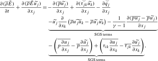 \begin{align}& \frac {\partial (\overline {\rho }\breve {E})}{\partial t} + \frac {\partial (\overline {\rho } \breve {E} \widetilde {u_j})}{\partial x_j} = - \frac {\partial (\overline {p}\widetilde {u_j})}{\partial x_j} + \frac {\partial (\overset {\smile } {\tau _{jk}}\widetilde {u_k})}{\partial x_j} - \frac {\partial \overset {\smile }{q_j}}{\partial x_j} \nonumber \\ &\qquad\qquad\qquad\qquad\quad \underbrace { - \widetilde {u_j} \frac {\partial }{\partial x_k} \left ( \overline {\rho } \widetilde {u_j u_k} - \overline {\rho } \widetilde {u_j} \widetilde {u_k} \right ) - \frac {1}{\gamma - 1} \frac {\partial (\overline {p u_j} - \overline {p}\widetilde {u_j})}{\partial x_j}}_{\text{SGS terms}} \nonumber \\ &\qquad\qquad\qquad\qquad\quad \underbrace { - \left (\overline {p \frac {\partial u_j}{\partial x_j}}- \overline {p} \frac {\partial \widetilde {u_j}}{\partial x_j} \right ) + \left ( \overline {\tau _{ik} \frac {\partial u_j}{\partial x_k}} - \overline {\tau _{jk}} \frac {\partial \widetilde {u_j}}{\partial x_k} \right )}_{\text{SGS terms}}, \end{align}
where the operators $\widetilde {(\cdot )}, (\cdot )^{\prime\prime}$
represent the density-weighted filtering operation,
$\widetilde {(\cdot )}, (\cdot )^{\prime\prime}$
represent the density-weighted filtering operation,
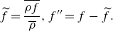 \begin{equation} \widetilde {f} = \frac {\overline {\rho f}}{\overline {\rho }}, f^{\prime\prime} = f - \widetilde {f}. \end{equation}
Here
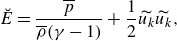 \begin{align}&\quad \breve {E} = \frac {\overline {p}}{\overline {\rho }(\gamma - 1)} + \frac {1}{2} \widetilde {u_k}\widetilde {u_k},\\[-10pt]\nonumber \end{align}
 \begin{align}&\quad\qquad \overset {\smile }{\tau _{ij}} = \mu (\widetilde {T}) \widetilde {S_{ij}},\\[-10pt]\nonumber \end{align}
 \begin{align}& \widetilde {S_{ij}} = \frac {\partial \widetilde {u_i}}{\partial x_j}+\frac {\partial \widetilde {u_j}}{\partial x_i} - \frac {2}{3} \delta _{ij} \frac {\partial \widetilde {u_k}}{\partial x_k},\\[-10pt]\nonumber \end{align}
 \begin{align}&\qquad\,\, \overset {\smile }{q_i} = - \kappa (\widetilde {T}) \frac {\partial \widetilde {T}}{\partial x_i}. \end{align}
The last term of (2.9) and the last four terms of (2.10) on the right-hand side are known as the SGS terms and cannot be computed from the resolved quantities (i.e. $\overline {f}$
and
$\overline {f}$
and $\widetilde {f}$
), therefore must be modelled using SGS models. As we focus on a low Mach number flow (
$\widetilde {f}$
), therefore must be modelled using SGS models. As we focus on a low Mach number flow ( $M \approx 0.1$
) with negligible SGS effects in (2.10) in this study, we focus on modelling the SGS term in (2.9).
$M \approx 0.1$
) with negligible SGS effects in (2.10) in this study, we focus on modelling the SGS term in (2.9).
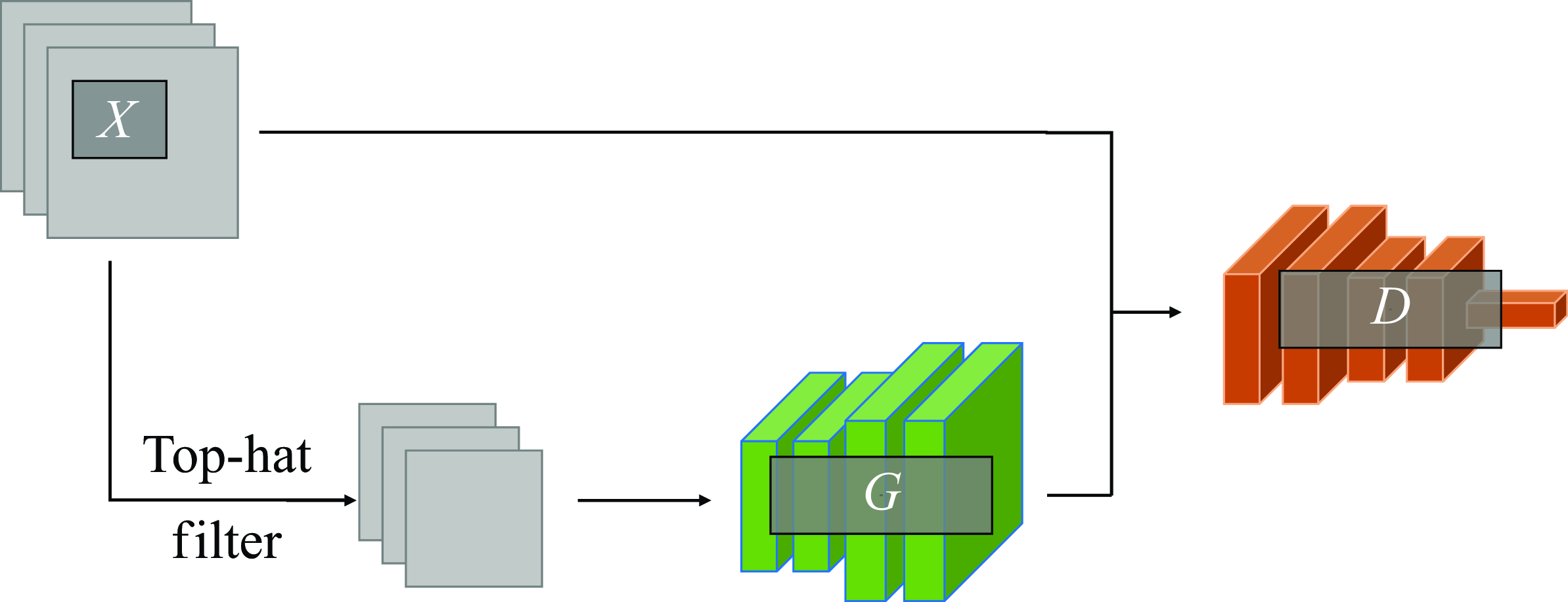
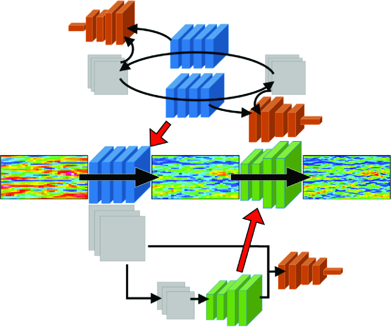
Figure 1. Schematic of supervised cGAN architecture: $G$
, generator model;
$G$
, generator model; $D$
, discriminator model;
$D$
, discriminator model; $X$
, training dataset.
$X$
, training dataset.
2.2. Machine learning
In this study, both supervised and unsupervised learning techniques are employed for the proposed pipeline method, as will be discussed in § 3. Here, the theoretical background for the GAN architectures that are employed in this study is discussed.
2.2.1. Conditional GAN
Conditional GAN (cGAN) (Mirza & Osindero Reference Mirza and Osindero2014) learns to generate data (output) from a given condition (input) from the annotated set of data. For the purposes of this study, cGAN can be considered as a mapping function that transforms the input data to the output. Numerous studies have extended cGAN for use in super-resolution (cf. the review by Tian et al. (Reference Tian, Zhang, Lin, Zuo, Zhang and Lin2022)), and is used in this study as the supervised machine learning model for super-resolution from fDNS data to DNS-quality flows. In the following, the employed formulation is described.
A schematic of the employed cGAN architecture is shown in figure 1. In cGAN used in this study, the generator network takes the low-resolution flow fields as input and tries to output the corresponding high-resolution flow fields. The discriminator takes either the output of the generator or the high-resolution (e.g. DNS) flow fields and tries to discern between the ‘real’ data in the training dataset (DNS data) and the generated ‘fake’ data (DNS-quality data generated by the generator). Because of the need to provide the corresponding high-resolution flow data for each low-resolution data as the paired training dataset, cGAN is classified as a supervised learning model.
To make the training procedure more stable, we employ Wasserstein GAN with gradient penalty (Gulrajani et al. Reference Gulrajani, Ahmed, Arjovsky, Dumoulin and Courville2017). Therefore, the loss function used in this study is as follows:
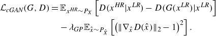 \begin{align} \mathcal{L}_{\textit{cGAN}}(G,D) &= \mathbb{E}_{x^{\textit{HR}} \sim P_{X}} \left [ D \big( x^{\textit{HR}} | x^{\textit{LR}} \big) - D \big( G \big( x^{\textit{LR}}\big) | x^{\textit{LR}} \big) \right ] \nonumber \\ &\quad - \lambda _{\textit{GP}} \mathbb{E}_{\hat {x} \sim P_{\hat {X}}} \left [ \left ( \| \nabla _{\hat {x}}D(\hat{x}) \|_2 - 1 \right ) ^2 \right ]. \end{align}
Here $G$
and
$G$
and $D$
are the generator and discriminator represented as a mapping function. Here
$D$
are the generator and discriminator represented as a mapping function. Here $D ( x^{\textit{HR}} | x^{\textit{LR}} )$
represents the output of the discriminator for the input
$D ( x^{\textit{HR}} | x^{\textit{LR}} )$
represents the output of the discriminator for the input $x^{\textit{HR}}$
, provided the condition
$x^{\textit{HR}}$
, provided the condition $x^{\textit{LR}}$
, where the superscripts ‘HR’ and ‘LR’ represent ‘high resolution’ and ‘low resolution’ respectively. Here
$x^{\textit{LR}}$
, where the superscripts ‘HR’ and ‘LR’ represent ‘high resolution’ and ‘low resolution’ respectively. Here $\mathbb{E}_{x\sim P_X} [ f(x) ]$
denotes the expected value of an arbitrary function
$\mathbb{E}_{x\sim P_X} [ f(x) ]$
denotes the expected value of an arbitrary function $f(x)$
when
$f(x)$
when $x$
is sampled from distribution
$x$
is sampled from distribution $X$
. In this study,
$X$
. In this study, $X$
represents the distribution of high-resolution data (DNS data), and
$X$
represents the distribution of high-resolution data (DNS data), and $x^{\textit{LR}}$
(filtered DNS data) is obtained by applying a top-hat filter to
$x^{\textit{LR}}$
(filtered DNS data) is obtained by applying a top-hat filter to $x^{\textit{HR}}$
. The first term is known as the adversarial loss. This loss encourages the discriminator to differentiate between real data and generated data more accurately, while the generator is led to be more able to deceive the discriminator. Here
$x^{\textit{HR}}$
. The first term is known as the adversarial loss. This loss encourages the discriminator to differentiate between real data and generated data more accurately, while the generator is led to be more able to deceive the discriminator. Here $\hat {x} \sim P_{\hat {X}}$
represents random samples from a random distribution
$\hat {x} \sim P_{\hat {X}}$
represents random samples from a random distribution $\hat {X}$
. Here
$\hat {X}$
. Here $\nabla _z f(z)$
is the partial derivative of
$\nabla _z f(z)$
is the partial derivative of $f(z)$
with respect to
$f(z)$
with respect to $z$
, and
$z$
, and $\|\cdot \|_2$
is the L2 norm. Here
$\|\cdot \|_2$
is the L2 norm. Here $\lambda _{\textit{GP}}$
is the constant weight coefficient for the last term, the gradient penalty loss, which constrains the discriminator to be a 1-Lipschitz function as is required in the Wasserstein GAN formulation. We found through preliminary experiments that for
$\lambda _{\textit{GP}}$
is the constant weight coefficient for the last term, the gradient penalty loss, which constrains the discriminator to be a 1-Lipschitz function as is required in the Wasserstein GAN formulation. We found through preliminary experiments that for $\lambda _{\textit{GP}} = 1, 10, 100$
, the results show no significant sensitivities, in which
$\lambda _{\textit{GP}} = 1, 10, 100$
, the results show no significant sensitivities, in which $\lambda _{\textit{GP}} = 10$
(recommended in the original paper (Gulrajani et al. Reference Gulrajani, Ahmed, Arjovsky, Dumoulin and Courville2017)) performs slightly better. Therefore, in this paper,
$\lambda _{\textit{GP}} = 10$
(recommended in the original paper (Gulrajani et al. Reference Gulrajani, Ahmed, Arjovsky, Dumoulin and Courville2017)) performs slightly better. Therefore, in this paper, $\lambda _{\textit{GP}}$
is set to
$\lambda _{\textit{GP}}$
is set to $10$
.
$10$
.
The process of learning the super-resolution mapping can be expressed as the following optimisation problem:
 \begin{equation} \arg \min _G \max _D \mathcal{L}_{\textit{cGAN}}(G,D). \end{equation}
The goal of this process is to obtain the super-resolution mapping $G$
that, given low-resolution data
$G$
that, given low-resolution data $x^{\textit{LR}}$
, predicts the high-resolution data, i.e.
$x^{\textit{LR}}$
, predicts the high-resolution data, i.e. $G (x^{\textit{LR}} ) \approx x^{\textit{HR}}$
. This is solved by iteratively updating the parameters of the networks according to the used optimiser algorithm.
$G (x^{\textit{LR}} ) \approx x^{\textit{HR}}$
. This is solved by iteratively updating the parameters of the networks according to the used optimiser algorithm.
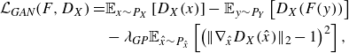
2.2.2. Cycle-consistency GAN
In this study, CycleGAN (Zhu et al. Reference Zhu, Park, Isola and Efros2020) is employed for the unsupervised learning of mappings between the vLES flows and fDNS flows. Figure 2 shows the schematic of a CycleGAN architecture. Here $X$
and
$X$
and $Y$
indicate the domains of data. In this study, they represent the vLES flow fields and fDNS flow fields, respectively. Unlike regular GAN architectures, a CycleGAN architecture consists of two generator networks (
$Y$
indicate the domains of data. In this study, they represent the vLES flow fields and fDNS flow fields, respectively. Unlike regular GAN architectures, a CycleGAN architecture consists of two generator networks ( $F, G$
) and two discriminator networks (
$F, G$
) and two discriminator networks ( $D_X, D_Y$
). Each generator is encouraged to learn a mapping that conserves the common characteristics between the two domains through the use of the cycle consistency loss. Mathematically, this process is understood as an optimisation problem of mapping functions
$D_X, D_Y$
). Each generator is encouraged to learn a mapping that conserves the common characteristics between the two domains through the use of the cycle consistency loss. Mathematically, this process is understood as an optimisation problem of mapping functions $F$
and
$F$
and $G$
between data distributions
$G$
between data distributions $X$
and
$X$
and $Y$
.
$Y$
.
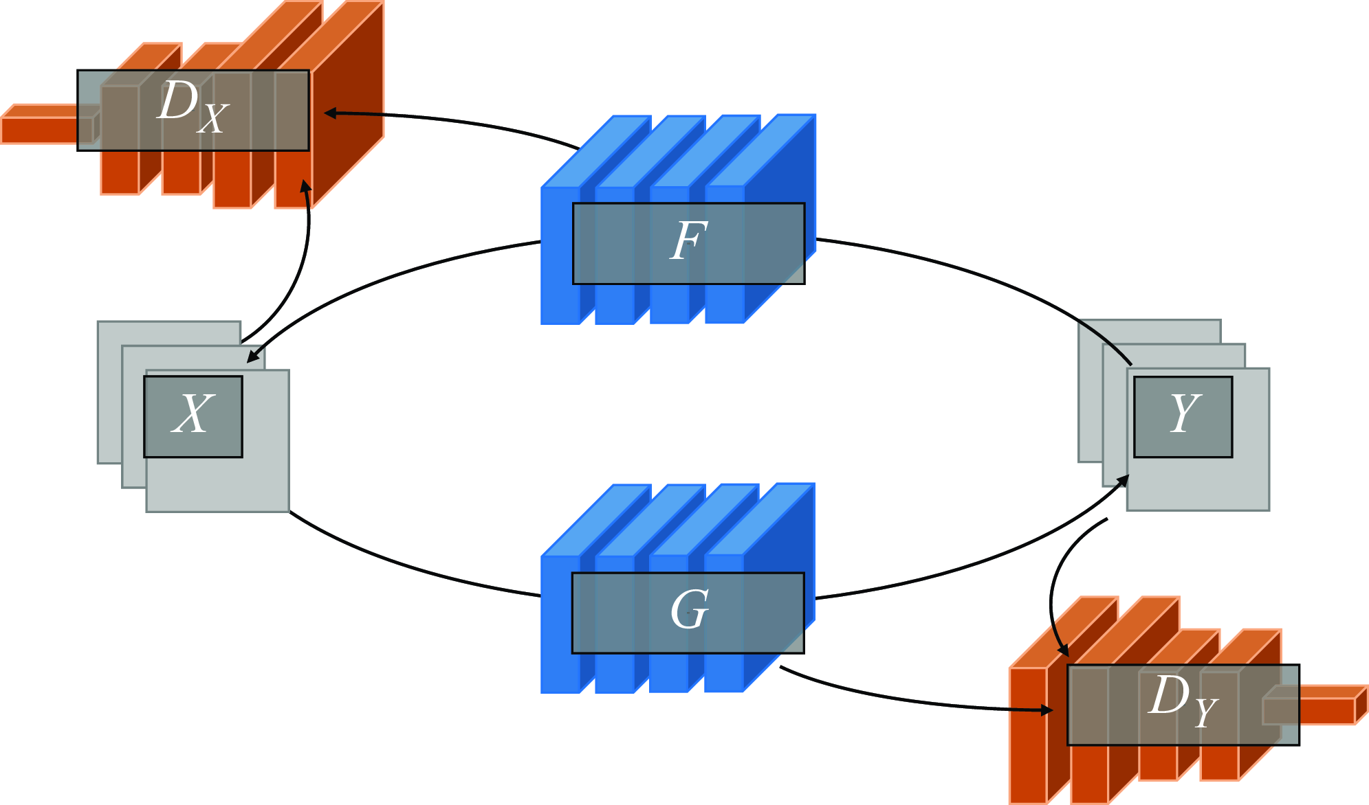
Figure 2. Schematic of unsupervised CycleGAN architecture: $F$
and
$F$
and $G$
, generator models;
$G$
, generator models; $D_X$
and
$D_X$
and $D_Y$
, discriminator models;
$D_Y$
, discriminator models; $X$
and
$X$
and $Y$
, training datasets.
$Y$
, training datasets.
The loss function used in this study is expressed as follows:
 \begin{equation} \mathcal{L}(F,G,D_X,D_Y)=\mathcal{L}_{\textit{GAN}}(F,D_X)+\mathcal{L}_{\textit{GAN}}(G,D_Y)+\lambda _{\textit{cyc}} \mathcal{L}_{\textit{cyc}}(F,G). \end{equation}
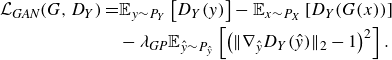
The first two terms of (2.18) are the adversarial losses defined as follows:
 \begin{align} \mathcal{L}_{\textit{GAN}}(F,D_X) =& \mathbb{E}_{x \sim P_X} \left [ D_X(x) \right ] -\mathbb{E}_{y\sim P_Y} \left [ D_X(F(y)) \right ] \nonumber \\ &- \lambda _{\textit{GP}} \mathbb{E}_{\hat {x} \sim P_{\hat {x}}} \left [ \left ( \| \nabla _{\hat {x}} D_X(\hat {x}) \| _2 - 1 \right )^2 \right ],\\[-10pt]\nonumber \end{align}
 \begin{align} \mathcal{L}_{\textit{GAN}}(G,D_Y) =& \mathbb{E}_{y \sim P_Y} \left [ D_Y(y) \right ] -\mathbb{E}_{x \sim P_X} \left [ D_Y(G(x)) \right ] \nonumber \\ &- \lambda _{\textit{GP}} \mathbb{E}_{\hat {y} \sim P_{\hat {y}}} \left [ \left ( \| \nabla _{\hat {y}} D_Y(\hat {y}) \| _2 - 1 \right )^2 \right ]. \end{align}
The adversarial losses are similar to the loss function of cGAN (2.16) except that they are not conditioned; i.e. the discriminators have only one input as opposed to two (input and condition) in cGAN. The third term of (2.18) is the cycle consistency loss, with a constant weight coefficient of $\lambda _{\textit{cyc}}=1$
. The cycle consistency loss is defined as
$\lambda _{\textit{cyc}}=1$
. The cycle consistency loss is defined as
 \begin{equation} \mathcal{L}_{\textit{cyc}}(F,G)=\mathbb{E}_{x \sim P_X}[\| F(G(x))-x\|_2]\\+\mathbb{E}_{y \sim P_Y}[\|G(F(y))-y\|_2)]. \end{equation}
This loss ensures that after data passes through the two generators, the original data are recovered; that is, $F(G(x)) \approx x$
and
$F(G(x)) \approx x$
and $G(F(y)) \approx y$
. This incentivises each mapping function
$G(F(y)) \approx y$
. This incentivises each mapping function $F$
and
$F$
and $G$
to retain the shared characteristics of the two datasets. The value of the weight coefficient
$G$
to retain the shared characteristics of the two datasets. The value of the weight coefficient $\lambda _{\textit{cyc}}$
was determined based on the preliminary experiments in which
$\lambda _{\textit{cyc}}$
was determined based on the preliminary experiments in which $\lambda _{\textit{cyc}} = 1$
performed better than the originally recommended value of
$\lambda _{\textit{cyc}} = 1$
performed better than the originally recommended value of $\lambda _{\textit{cyc}} = 10$
(Zhu et al. Reference Zhu, Park, Isola and Efros2020). The objective of the training phase is to find the model parameters that meet the following condition:
$\lambda _{\textit{cyc}} = 10$
(Zhu et al. Reference Zhu, Park, Isola and Efros2020). The objective of the training phase is to find the model parameters that meet the following condition:
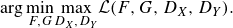 \begin{equation} \arg \underset {F,G}{\min } \underset {D_X, D_Y}{\max } \mathcal{L}(F,G,D_X,D_Y). \end{equation}
3. Methodology
The proposed machine-learning methodology to SGS modelling consists of mainly two steps: the super-resolution of the input vLES flow field by the machine learning pipeline and the extraction of SGS components from the super-resolved DNS-quality flow field. Each step is described in the following subsections.
3.1. Machine-learning pipeline
Here we describe the proposed machine-learning-based super-resolution pipeline. The pipeline consists of two parts: the vLES-to-fDNS model ( $G_{\textit{vLES}-\textit{fDNS}}$
) that converts vLES velocity data to the data of fDNS quality, and the super-resolution model (
$G_{\textit{vLES}-\textit{fDNS}}$
) that converts vLES velocity data to the data of fDNS quality, and the super-resolution model ( $G_{\textit{SR}}$
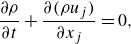
) that converts the fDNS-quality velocity data to the desired DNS quality data. Figure 3 illustrates the architecture of the pipeline. The vLES-to-fDNS model
$G_{\textit{SR}}$
) that converts the fDNS-quality velocity data to the desired DNS quality data. Figure 3 illustrates the architecture of the pipeline. The vLES-to-fDNS model $G_{\textit{vLES}-\textit{fDNS}}$
(figure 3
a) is obtained as one of the generators in the CycleGAN (
$G_{\textit{vLES}-\textit{fDNS}}$
(figure 3
a) is obtained as one of the generators in the CycleGAN ( $G$
in § 2.2.2). Since the pairs of instantaneous flow fields for vLES and fDNS are unobtainable, learning the mapping between vLES and fDNS must be performed in an unsupervised manner, as discussed in § 1. Therefore, this model is trained and runs inference on vLES and fDNS data. The super-resolution model
$G$
in § 2.2.2). Since the pairs of instantaneous flow fields for vLES and fDNS are unobtainable, learning the mapping between vLES and fDNS must be performed in an unsupervised manner, as discussed in § 1. Therefore, this model is trained and runs inference on vLES and fDNS data. The super-resolution model $G_{\textit{SR}}$
(figure 3
b) is trained using fDNS flow fields to obtain the original DNS flow fields that are before the filtering operation. In this study, the model is obtained by cGAN. The proposed pipeline (figure 3
c) combines the two constructed models. In the pipeline, the fDNS-quality output of the vLES-to-fDNS model
$G_{\textit{SR}}$
(figure 3
b) is trained using fDNS flow fields to obtain the original DNS flow fields that are before the filtering operation. In this study, the model is obtained by cGAN. The proposed pipeline (figure 3
c) combines the two constructed models. In the pipeline, the fDNS-quality output of the vLES-to-fDNS model $G_{\textit{vLES}-\textit{fDNS}}$
is used as the input to the super-resolution model
$G_{\textit{vLES}-\textit{fDNS}}$
is used as the input to the super-resolution model $G_{\textit{SR}}$
to accurately perform the super-resolution. To summarise, the super-resolved flow field of DNS quality data are obtained by sequentially processing the vLES data through the two models as
$G_{\textit{SR}}$
to accurately perform the super-resolution. To summarise, the super-resolved flow field of DNS quality data are obtained by sequentially processing the vLES data through the two models as
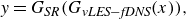 \begin{equation} y = G_{\textit{SR}}(G_{\textit{vLES}-\textit{fDNS}}(x)), \end{equation}
where $x$
represents the input velocity data of the vLES and
$x$
represents the input velocity data of the vLES and $y$
represents the output DNS-quality velocity data.
$y$
represents the output DNS-quality velocity data.
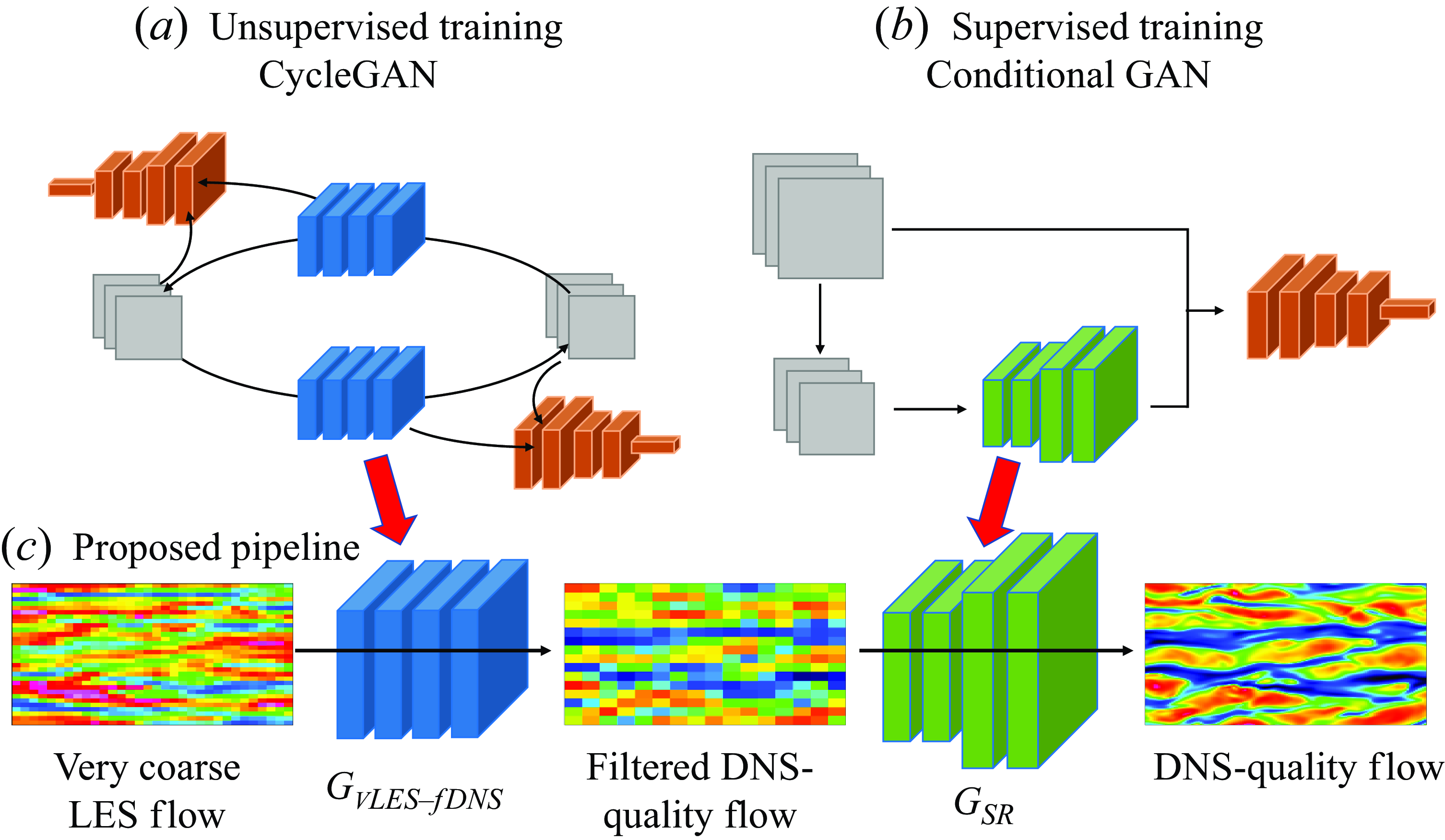
Figure 3. Schematic of the proposed unsupervised–supervised machine learning pipeline (c). The first model is taken from an unsupervisedly trained CycleGAN model (a), and the second model is from a supervisedly trained conditional GAN model (b). Blue and green models, generators; orange models, discriminators; grey squares, training data.
It should be noted that we have first attempted to train a single model to achieve the above super-resolution problem, that is, we train a vLES-to-DNS model using CycleGAN with vLES and DNS data as the training data. However the training did not properly converge, and the resulting model’s performance was unsatisfactory. We believe that the difficulty originates from the training process of the CycleGAN architecture, in which the four constituent machine-learning models (shown in figure 2) must learn at a similar pace for the duration of the training process. When vLES and DNS are used as the training data for the CycleGAN, the different numbers of grid points in the two datasets lead to an unbalanced training process which degrades the convergence of the trained models. Similar findings regarding using multiple models were also reported in other studies, such as unsupervised super-resolution of natural images (Lugmayr, Danelljan & Timofte Reference Lugmayr, Danelljan and Timofte2019), and spatiotemporal super-resolution of fluid flow (Fukami, Fukagata & Taira Reference Fukami, Fukagata and Taira2021).
We stress that for SGS modelling in vLES, the unsupervised vLES-to-fDNS model is crucial for accurate predictions of SGS stresses. The idea stems from the fact that because vLES does not sufficiently resolve the energetic eddies, the resolved scales of turbulence is not accurate; that is, the resolved flow fields are not equivalent to the filtered DNS (i.e. vLES $\neq$
fDNS). Therefore, typical supervised super-resolution models which are trained on fDNS and DNS are not applicable to the super-resolution of vLES. It is thus necessary to first convert the vLES flow fields to fDNS-quality flow fields before inputting into the super-resolution model. This machine learning process must be performed by an unsupervised model because it is impossible to obtain the pairs of vLES (input) and fDNS (expected output), as discussed in § 1. This class of problem is sometimes classified as ‘style transfer’ using unpaired datasets. While there exist many other methods that also accomplish the same task (e.g. CUT (Park et al. Reference Park, Efros, Zhang and Zhu2020) and DCLGAN (Han et al. Reference Han, Shoeiby, Petersson and Armin2021)), CycleGAN (Zhu et al. Reference Zhu, Park, Isola and Efros2020) enables such unsupervised learning through a relatively simple architecture, and, as will be shown later in § 5.1, CycleGAN is effective for the vLES-to-fDNS model.
$\neq$
fDNS). Therefore, typical supervised super-resolution models which are trained on fDNS and DNS are not applicable to the super-resolution of vLES. It is thus necessary to first convert the vLES flow fields to fDNS-quality flow fields before inputting into the super-resolution model. This machine learning process must be performed by an unsupervised model because it is impossible to obtain the pairs of vLES (input) and fDNS (expected output), as discussed in § 1. This class of problem is sometimes classified as ‘style transfer’ using unpaired datasets. While there exist many other methods that also accomplish the same task (e.g. CUT (Park et al. Reference Park, Efros, Zhang and Zhu2020) and DCLGAN (Han et al. Reference Han, Shoeiby, Petersson and Armin2021)), CycleGAN (Zhu et al. Reference Zhu, Park, Isola and Efros2020) enables such unsupervised learning through a relatively simple architecture, and, as will be shown later in § 5.1, CycleGAN is effective for the vLES-to-fDNS model.
We also note that, with an artificial modification function $g$
such that
$g$
such that $g(\textrm {DNS}) \approx \textrm{vLES}$
, we may supervisedly train a machine learning model using the one-to-one corresponding pairs of
$g(\textrm {DNS}) \approx \textrm{vLES}$
, we may supervisedly train a machine learning model using the one-to-one corresponding pairs of $g(\textrm {DNS})$
and DNS flow fields as the training data. Such training procedure would allow for a supervised machine learning model to perform the accurate super-resolution from vLES to DNS. However, the effects of errors caused by coarse grid resolutions are not well understood to construct such function
$g(\textrm {DNS})$
and DNS flow fields as the training data. Such training procedure would allow for a supervised machine learning model to perform the accurate super-resolution from vLES to DNS. However, the effects of errors caused by coarse grid resolutions are not well understood to construct such function $g$
today. Therefore, we must resort to unsupervised learning methods to train machine learning models that can take vLES flow fields as the input.
$g$
today. Therefore, we must resort to unsupervised learning methods to train machine learning models that can take vLES flow fields as the input.
The choice of cGAN as the supervised super-resolution model as opposed to a simple neural network (using the L2 error as the loss function, for example) is based on the reports that GANs show better predictions of small-scale turbulent structures (Güemes et al. Reference Güemes, Discetti, Ianiro, Sirmacek, Azizpour and Vinuesa2021; Kim et al. Reference Kim, Kim, Won and Lee2021). The same tendencies are obtained using the dataset of this study; cGAN shows better agreement of the small-scale structures compared with a simple convolutional neural network (CNN). As accurate predictions of small structures are key to accurate predictions of SGS stresses, we employ the cGAN in this study.
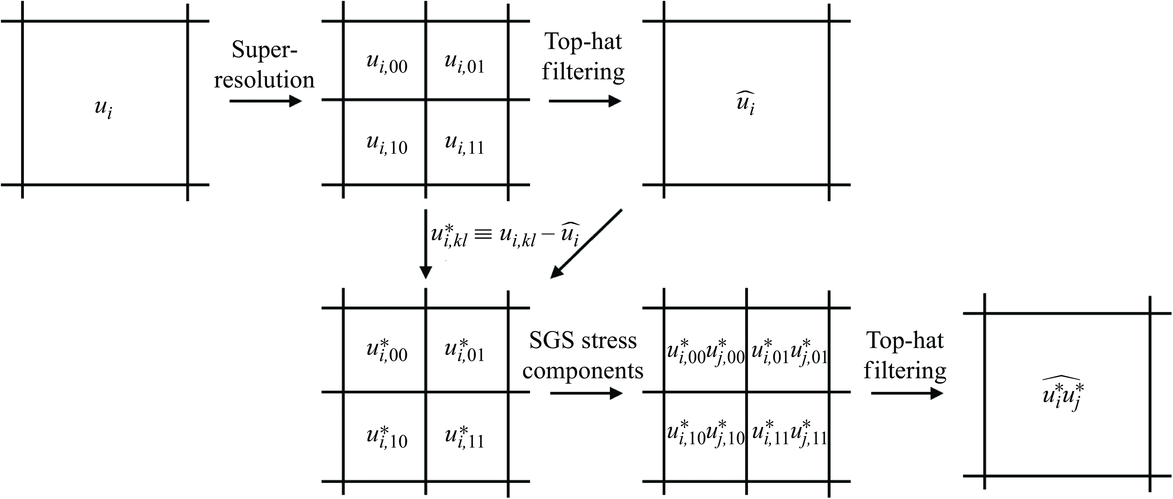
Figure 4. Schematic of the SGS extraction process. Figure shows the process for $m=2$
.
$m=2$
.
3.2. Extraction of SGS components
To utilise the super-resolved flow obtained by the proposed pipeline as an SGS model, the small-scale unresolved turbulence reconstructed by the super-resolution pipeline is extracted as SGS stress components. Figure 4 illustrates this process. Consider that the two-dimensional distributions of the three components of velocity $u_i \in \mathbb{R}^{H \times W \times 3}$
on a grid of
$u_i \in \mathbb{R}^{H \times W \times 3}$
on a grid of $H \times W$
points (where
$H \times W$
points (where $(u_1,u_2,u_3) = (u,v,w)$
, the three components of velocity) is super-resolved by a factor of
$(u_1,u_2,u_3) = (u,v,w)$
, the three components of velocity) is super-resolved by a factor of $m$
. The super-resolved flow field is expressed as the distribution on a
$m$
. The super-resolved flow field is expressed as the distribution on a $mH \times mW$
grid as
$mH \times mW$
grid as $u^{\textit{SR}}_{i, kl} \in \mathbb{R}^{mH \times mW \times 3}$
. Here, the subscripts
$u^{\textit{SR}}_{i, kl} \in \mathbb{R}^{mH \times mW \times 3}$
. Here, the subscripts $1 \leqq k,l \leqq m$
indicate the position of a super-resolved grid point within the given original coarse grid point. In other words, the space occupied by a single grid point of the vLES is now occupied by
$1 \leqq k,l \leqq m$
indicate the position of a super-resolved grid point within the given original coarse grid point. In other words, the space occupied by a single grid point of the vLES is now occupied by $m^2$
grid points of the super-resolved velocity field. Applying a top-hat filter
$m^2$
grid points of the super-resolved velocity field. Applying a top-hat filter $\widehat {(\cdot )}$
to the output velocity field
$\widehat {(\cdot )}$
to the output velocity field $u^{\textit{SR}}_{i,kl}$
yields the filtered velocity components
$u^{\textit{SR}}_{i,kl}$
yields the filtered velocity components $\widehat {u_{i}} \in \mathbb{R}^{H \times W \times 3}$
and fluctuations
$\widehat {u_{i}} \in \mathbb{R}^{H \times W \times 3}$
and fluctuations $u_{i,kl}^* \equiv u^{\textit{SR}}_{i,kl} - \widehat {u_i} \in \mathbb{R}^{mH \times mW \times 3}$
. Local SGS stress components can then be calculated as
$u_{i,kl}^* \equiv u^{\textit{SR}}_{i,kl} - \widehat {u_i} \in \mathbb{R}^{mH \times mW \times 3}$
. Local SGS stress components can then be calculated as $- u_{i,kl}^* u_{j,kl}^* \in \mathbb{R}^{mH \times mW \times 3 \times 3}$
. Finally, applying a top-hat filter to the local SGS stresses yields the SGS stress components
$- u_{i,kl}^* u_{j,kl}^* \in \mathbb{R}^{mH \times mW \times 3 \times 3}$
. Finally, applying a top-hat filter to the local SGS stresses yields the SGS stress components $\tau _{\textit{ij}, \textit{SGS}} \equiv - \widehat {u_i^* u_j^*} \in \mathbb{R}^{H \times W \times 3 \times 3}$
, which will then be used as the SGS stress terms in (2.9) in the computational fluid dynamics solver. In actuality, because
$\tau _{\textit{ij}, \textit{SGS}} \equiv - \widehat {u_i^* u_j^*} \in \mathbb{R}^{H \times W \times 3 \times 3}$
, which will then be used as the SGS stress terms in (2.9) in the computational fluid dynamics solver. In actuality, because $\tau _{\textit{ij}, \textit{SGS}} = \tau _{ji, {\textit{SGS}}}$
is satisfied, the SGS stress tensor
$\tau _{\textit{ij}, \textit{SGS}} = \tau _{ji, {\textit{SGS}}}$
is satisfied, the SGS stress tensor $\tau _{\textit{ij}, \textit{SGS}}$
has
$\tau _{\textit{ij}, \textit{SGS}}$
has $H \times W \times 6$
degrees of freedom.
$H \times W \times 6$
degrees of freedom.
During the simulation (results presented in § 6 and § 7), the clipped SGS stress $\tau _{\textit{ij}, \textit{SGS}}^{\textit{clip}}$
is used for numerical stability according to the following equations:
$\tau _{\textit{ij}, \textit{SGS}}^{\textit{clip}}$
is used for numerical stability according to the following equations:
 \begin{align} \tau _{\textit{ij}, \textit{SGS}}^{\textit{clip}} &\equiv \left \{ \begin{matrix} \tau _{\textit{ij}, \textit{SGS}} & \textrm {if} \: \mu _{\textit{eff}} \gt \mu _{\textit{clip}}, \\ \tau _{\textit{ij}, \textit{SGS}} - \left ( 1 - \frac {\mu _{\textit{clip}}}{\mu _{\textit{eff}}} \right ) \mu _{\textit{eff}} S_{ij} & \textrm {otherwise.} \end{matrix} \right . \nonumber ,\\ \mu _{\textit{eff}} &\equiv \frac {\sum _{ij} \tau _{\textit{ij}, \textit{SGS}} \frac {\partial u_i}{\partial x_j} } { \sum _{ij} S_{ij} \frac {\partial u_i}{\partial x_j}} . \end{align}
Here, $S_{ij}$
is the deviatoric part of the strain tensor as in (2.6) and
$S_{ij}$
is the deviatoric part of the strain tensor as in (2.6) and $\mu _{\textit{clip}} \leqq 0$
is given as the simulation parameter. The clipping procedure is designed to bound the minimum possible effective viscosity by
$\mu _{\textit{clip}} \leqq 0$
is given as the simulation parameter. The clipping procedure is designed to bound the minimum possible effective viscosity by $\mu _{\textit{clip}}$
. As a result, only the most extreme and rare localised energy backscatter events (i.e. very large negative
$\mu _{\textit{clip}}$
. As a result, only the most extreme and rare localised energy backscatter events (i.e. very large negative $\mu _{\textit{eff}}$
) that may destabilise the simulation but are physically important for the accurate simulation of turbulence are weakened to a moderate backscatter. In this study, the parameter is set to
$\mu _{\textit{eff}}$
) that may destabilise the simulation but are physically important for the accurate simulation of turbulence are weakened to a moderate backscatter. In this study, the parameter is set to $\mu _{\textit{clip}} / \overline {\mu }_w \approx -2$
. We note that it is desirable to set the value of
$\mu _{\textit{clip}} / \overline {\mu }_w \approx -2$
. We note that it is desirable to set the value of $\mu _{\textit{clip}}$
as low as possible to minimise the amount of backscatter that is clipped in the simulation while ensuring its stability. The sensitivity of the results against the value of
$\mu _{\textit{clip}}$
as low as possible to minimise the amount of backscatter that is clipped in the simulation while ensuring its stability. The sensitivity of the results against the value of $\mu _{\textit{clip}}$
is shown in Appendix C.
$\mu _{\textit{clip}}$
is shown in Appendix C.
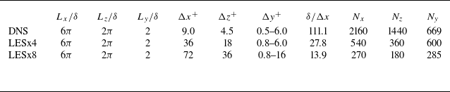
Table 1. List of parameters for each computational set-up. $L_x$
,
$L_x$
, $L_z$
and
$L_z$
and $L_y$
denote computational domain size. Here
$L_y$
denote computational domain size. Here $\Delta x$
,
$\Delta x$
, $\Delta y$
and
$\Delta y$
and $\Delta z$
denote grid resolutions in each direction, and superscript
$\Delta z$
denote grid resolutions in each direction, and superscript $(\cdot )^+$
represents values in wall units. Here
$(\cdot )^+$
represents values in wall units. Here $N_x$
,
$N_x$
, $N_z$
and
$N_z$
and $N_y$
denote number of grid points in each direction.
$N_y$
denote number of grid points in each direction.
4. Dataset generation and training process
4.1. Simulation settings for dataset generation
To train our proposed machine-learning-based SGS modelling methodology, the data from DNS and LES of a fully developed turbulent channel flow are obtained by the well-validated compressible flow solver (Kawai & Fujii Reference Kawai and Fujii2008; Asada & Kawai Reference Asada and Kawai2018; Kawai Reference Kawai2019; Hirai, Pecnik & Kawai Reference Hirai, Pecnik and Kawai2021; Kamogawa, Tamaki & Kawai Reference Kamogawa, Tamaki and Kawai2023; Tamaki & Kawai Reference Tamaki and Kawai2023). As discussed in § 2.1, DNS solves (2.1)–(2.3), while LES solves (2.8)–(2.10).
The parameters of the computational grids are summarised in table 1. A uniform grid in the streamwise direction $x$
and spanwise direction
$x$
and spanwise direction $z$
is used for both the DNS and LES; the DNS grid spacings are
$z$
is used for both the DNS and LES; the DNS grid spacings are $(\Delta x^+, \Delta z^+) \approx (9.0,4.5)$
, and the LES grid spacings are four times (
$(\Delta x^+, \Delta z^+) \approx (9.0,4.5)$
, and the LES grid spacings are four times ( $(\Delta x^+, \Delta z^+) \approx (36, 18)$
) and eight times (
$(\Delta x^+, \Delta z^+) \approx (36, 18)$
) and eight times ( $(\Delta x^+, \Delta z^+) \approx (72, 36)$
) that of the DNS for LESx4 and LESx8 cases, respectively. The DNS grid spacings are comparable to the previous studies by Lee & Moser (Reference Lee and Moser2015). Here the superscript
$(\Delta x^+, \Delta z^+) \approx (72, 36)$
) that of the DNS for LESx4 and LESx8 cases, respectively. The DNS grid spacings are comparable to the previous studies by Lee & Moser (Reference Lee and Moser2015). Here the superscript $(\cdot )^+$
denotes quantities in wall units. We have confirmed that the present DNS grid shows grid convergence in terms of the turbulent statistics studied in this study. The grid spacings of LESx4 are roughly comparable to the conventional LES, while LESx8 corresponds to the vLES targeted in this study. The Reynolds number based on the channel half-width
$(\cdot )^+$
denotes quantities in wall units. We have confirmed that the present DNS grid shows grid convergence in terms of the turbulent statistics studied in this study. The grid spacings of LESx4 are roughly comparable to the conventional LES, while LESx8 corresponds to the vLES targeted in this study. The Reynolds number based on the channel half-width $\delta$
and bulk velocity
$\delta$
and bulk velocity $u_b$
is set as
$u_b$
is set as $Re_{b, \delta } \approx 20000$
, which gives the friction Reynolds number
$Re_{b, \delta } \approx 20000$
, which gives the friction Reynolds number $Re_\tau \approx 1000$
. The bulk Mach number is set as
$Re_\tau \approx 1000$
. The bulk Mach number is set as $M_b = u_b / \overline {a}_w \approx 0.1$
, where
$M_b = u_b / \overline {a}_w \approx 0.1$
, where $a_w$
is the speed of sound at the wall. The flow is driven by a constant body force in the streamwise direction as
$a_w$
is the speed of sound at the wall. The flow is driven by a constant body force in the streamwise direction as $s = \tau _w / \delta$
, where
$s = \tau _w / \delta$
, where $\tau _w$
is the skin friction estimated by Dean’s empirical correlation (Dean Reference Dean1978) as
$\tau _w$
is the skin friction estimated by Dean’s empirical correlation (Dean Reference Dean1978) as
 \begin{equation} C_f = \frac {\tau _w}{\dfrac{1}{2} \rho _b u_b^2} = 0.073 Re_{b, 2\delta }^{-0.25}. \end{equation}
Here, the bulk density $\rho _b$
is given as the initial state. The constant body force fixes the wall shear stress
$\rho _b$
is given as the initial state. The constant body force fixes the wall shear stress $\tau _w$
and the friction Reynolds number
$\tau _w$
and the friction Reynolds number $Re_\tau$
to a constant so that the near-wall grid resolution in wall units is the same between the different computational set-ups. This method of applying a constant body force has been compared with other methods (constant flow rate and constant power input) and, for the purposes of this study, has negligible effects on the flow fields (Quadrio, Frohnapfel & Hasegawa Reference Quadrio, Frohnapfel and Hasegawa2016). The adiabatic non-slip boundary condition is applied at the walls, and the periodic boundary condition is applied in the streamwise and spanwise directions.
$Re_\tau$
to a constant so that the near-wall grid resolution in wall units is the same between the different computational set-ups. This method of applying a constant body force has been compared with other methods (constant flow rate and constant power input) and, for the purposes of this study, has negligible effects on the flow fields (Quadrio, Frohnapfel & Hasegawa Reference Quadrio, Frohnapfel and Hasegawa2016). The adiabatic non-slip boundary condition is applied at the walls, and the periodic boundary condition is applied in the streamwise and spanwise directions.
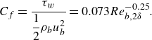
Figure 5. Mean streamwise velocity (a) and Reynolds stresses (b) of DNS, LESx4 and LESx8. Here circles, DNS; dashed lines, LESx4; solid lines, LESx8. For (b) blue, streamwise Reynolds normal stress ( $\overline {u^{\prime}u^{\prime}}$
); orange, wall-normal Reynolds normal stress (
$\overline {u^{\prime}u^{\prime}}$
); orange, wall-normal Reynolds normal stress ( $\overline {v^{\prime}v^{\prime}}$
); green, spanwise Reynolds normal stress (
$\overline {v^{\prime}v^{\prime}}$
); green, spanwise Reynolds normal stress ( $\overline {w^{\prime}w^{\prime}}$
); red, Reynolds shear stress (
$\overline {w^{\prime}w^{\prime}}$
); red, Reynolds shear stress ( $\overline {u^{\prime}v^{\prime}}$
).
$\overline {u^{\prime}v^{\prime}}$
).
The third-order total variation diminishing Runge–Kutta method (Gottlieb & Shu Reference Gottlieb and Shu1998) is used for time integration. The second-order kinetic energy and entropy preserving (KEEP) scheme (Kuya, Totani & Kawai Reference Kuya, Totani and Kawai2018) is used for spatial discretisation. The KEEP scheme is a split-form-based non-dissipative central scheme and achieves robust computation without introducing numerical dissipations, and thus there is no dissipation error in the DNS and LES. While the results of an LES should not depend on the employed discretisation scheme, this issue is important for vLES in which the energetic eddies are intended to be not resolved well, leading to discretisation errors involved in the solutions. Therefore, in this study, we employ the KEEP scheme whose non-dissipative and robust characteristics have been shown to be effective for the LES (Asada et al. Reference Asada, Tamaki, Takaki, Yumitori, Tamura, Hatanaka, Imai, Maeyama and Kawai2023). We also emphasise that the non-dissipative characteristic is highly desirable for the very coarse LES to discuss the effects of different SGS models as the SGS dissipation is not contaminated by the numerical dissipation. The selective mixed-scale SGS model (Lenormand et al. Reference Lenormand, Sagaut, Phuoc and Comte2000) is used as the SGS model for the LES.
Figure 5 shows the mean streamwise velocity and the Reynolds stresses obtained by the DNS, LESx4 and LESx8. The LESx4 reproduces the mean streamwise velocity of DNS well, whereas LESx8 overestimates the velocity. Similarly in the Reynolds stresses, LESx4 agrees well with the DNS while LESx8 shows deviations from the DNS. The discrepancies in the vLES (i.e. LESx8) make learning the mappings difficult as the machine learning model must also learn to significantly adjust the means and variances from the input data.
In the tests, LESx4 serves as the baseline conventional LES case where the resolved turbulent statistics agree reasonably well with the DNS. On the other hand, LESx8 serves as the very coarse-grid case where correct turbulence must be predicted from erroneous resolved turbulent fields. Considering the spanwise wavelength of the near-wall streak structures at $\lambda _z^+ \approx 100$
(Smith & Metzler Reference Smith and Metzler1983), LESx8 (vLES) places two to three grid points per wavelength of the near-wall streaks.
$\lambda _z^+ \approx 100$
(Smith & Metzler Reference Smith and Metzler1983), LESx8 (vLES) places two to three grid points per wavelength of the near-wall streaks.
4.2. Training settings
In the simulations of wall turbulence, a grid that is uniform in the wall-parallel directions and non-uniform in the wall-normal direction is often used. Convolution in the wall-normal direction may be unsuitable because the convolution operation expects that the grid resolution does not change between training and inference; this is not the case with non-uniform grids when the flow condition (such as the Reynolds number) changes. Therefore, we choose to super-resolve each wall-parallel plane separately, then combine the results to reconstruct the entire three-dimensional flow fields.
To learn the two-dimensional super-resolution mapping that works throughout the channel, eight wall-parallel planes at different distances from the wall are chosen as the training data: four from the inner layer scaling ( $y^+ \approx 5, 15, 30, 100$
) and four from the outer layer scaling (
$y^+ \approx 5, 15, 30, 100$
) and four from the outer layer scaling ( $y/\delta = 0.25, 0.50, 0.75, 1.00$
). The slices at
$y/\delta = 0.25, 0.50, 0.75, 1.00$
). The slices at $y^+ \approx 5, 15, 30, 100$
correspond to
$y^+ \approx 5, 15, 30, 100$
correspond to $y/\delta = 0.005, 0.015, 0.03, 0.1$
, respectively. As the various flow characteristics of the turbulent channel are included in the training data, the wall-parallel planes that are not included in the training data are expected to be treated as an interpolation between the learned turbulent structures. As the employed Mach number is low in this study (
$y/\delta = 0.005, 0.015, 0.03, 0.1$
, respectively. As the various flow characteristics of the turbulent channel are included in the training data, the wall-parallel planes that are not included in the training data are expected to be treated as an interpolation between the learned turbulent structures. As the employed Mach number is low in this study ( $M_b \approx 0.1$
), the contributions of compressibility to the flow are negligible and the temperature can be considered as a passive scalar. Therefore, the three components of velocity (
$M_b \approx 0.1$
), the contributions of compressibility to the flow are negligible and the temperature can be considered as a passive scalar. Therefore, the three components of velocity ( $u,v,w$
) are considered for training and prediction to obtain the SGS stress components.
$u,v,w$
) are considered for training and prediction to obtain the SGS stress components.
As the turbulent channel is symmetric about the centreline, instantaneous snapshots from both walls of the channel are collected to obtain the training data. Here 1600 snapshots from each of the $x{-}z$
planes are used as the training data, that is, a total of 25 600 snapshots (1600 snapshots
$x{-}z$
planes are used as the training data, that is, a total of 25 600 snapshots (1600 snapshots $\times$
8 planes
$\times$
8 planes $\times$
2 walls) for both DNS and LES. The snapshots are taken every
$\times$
2 walls) for both DNS and LES. The snapshots are taken every $\Delta t ^ + \approx 2.9$
. Here 40 snapshots independent from the training data are used to create the results shown in the following § 5. As discussed in § 3.1, the unsupervised training (figure 3
a) requires vLES and fDNS flow fields, while the supervised training (figure 3
b) requires fDNS and DNS flow fields as the training dataset. The fDNS flow fields in the datasets are obtained by applying a top-hat filter and downsampling the DNS flow fields in the streamwise and spanwise directions. During the training for the LESx4, random patches of
$\Delta t ^ + \approx 2.9$
. Here 40 snapshots independent from the training data are used to create the results shown in the following § 5. As discussed in § 3.1, the unsupervised training (figure 3
a) requires vLES and fDNS flow fields, while the supervised training (figure 3
b) requires fDNS and DNS flow fields as the training dataset. The fDNS flow fields in the datasets are obtained by applying a top-hat filter and downsampling the DNS flow fields in the streamwise and spanwise directions. During the training for the LESx4, random patches of $256 \times 256$
grid points from the DNS snapshots and
$256 \times 256$
grid points from the DNS snapshots and $64 \times 64$
grid points from the LESx4 snapshots are used with zero-padding for the convolution operation. These patches correspond to the size of
$64 \times 64$
grid points from the LESx4 snapshots are used with zero-padding for the convolution operation. These patches correspond to the size of $2.304 \delta \times 1.152 \delta$
in physical space. This choice is because the size of the largest structures in turbulent channel flow scales with
$2.304 \delta \times 1.152 \delta$
in physical space. This choice is because the size of the largest structures in turbulent channel flow scales with $\delta$
(Liu, Adrian & Hanratty Reference Liu, Adrian and Hanratty2001), and the patches with a size of at least
$\delta$
(Liu, Adrian & Hanratty Reference Liu, Adrian and Hanratty2001), and the patches with a size of at least $\delta \times \delta$
is required during the training to capture the large-scale structures in the outer-layer regions. Likewise in the training of LESx8, random patches of
$\delta \times \delta$
is required during the training to capture the large-scale structures in the outer-layer regions. Likewise in the training of LESx8, random patches of $32 \times 32$
grid points are used for consistency. During testing, however, the snapshots for the full computational domain are used as inputs, i.e.
$32 \times 32$
grid points are used for consistency. During testing, however, the snapshots for the full computational domain are used as inputs, i.e. $540 \times 360$
grid points for LESx4 and
$540 \times 360$
grid points for LESx4 and $270 \times 180$
grid points for LESx8. Periodic padding is used during testing so that the periodic boundary condition of the turbulent channel is satisfied by the output flow field.
$270 \times 180$
grid points for LESx8. Periodic padding is used during testing so that the periodic boundary condition of the turbulent channel is satisfied by the output flow field.
All networks in this study are two-dimensional fully convolutional networks. The detailed architectures of each network are shown in Appendix A. Adam (Kingma & Ba Reference Kingma and Ba2014) with $\alpha =10^{-5}$
,
$\alpha =10^{-5}$
, $\beta _1=0.5$
is employed as the optimisers for all networks. The learning rate is
$\beta _1=0.5$
is employed as the optimisers for all networks. The learning rate is $10^{-5}$
, and a batch size of
$10^{-5}$
, and a batch size of $16$
is used.
$16$
is used.
The convention in the machine learning community is to normalise the input and output data to have zero mean and unit standard deviation. However, this process requires prior knowledge of the output distributions, which is not always available as the DNS data. Therefore, in this study, both input and output data are normalised by the mean and standard deviation of the input for each off-wall distance. With this normalisation method, the output data do not always have zero mean and unit standard deviation. In particular, the input velocities at the non-slip wall boundary are always zero; that is, the mean and standard deviation of the input data are zero. To undo the normalisation of the machine-learning output for the velocities at the wall, the output velocities are multiplied by the input standard deviation of zero, which always produces zero velocity as the output. Therefore, the non-slip boundary conditions at the walls are satisfied by the output flow field.
5. Validation of machine learning pipeline
In this section, we perform the a priori test of the proposed unsupervised–supervised machine learning pipeline, and the predicted turbulent flows and statistics are discussed. The SGS stresses are also extracted from the super-resolved flow fields and compared with the reference data. Here, to test whether the machine-learning pipeline is trained appropriately to predict the SGS stress components, we use the precomputed flow field from the LES using a conventional SGS model (selective mixed-scale model in this study) at the friction Reynolds number of $Re_\tau \approx 1000$
(same as the training data) as the input of the proposed pipeline and test the prediction accuracy for each of the pipeline component. Here 40 instantaneous snapshots that are independent from the training data are used to produce the results in this section, as discussed in § 4.2. For brevity, we only show the results of the models for LESx8 as a vLES case in this section. We note that the proposed pipeline also works well for LESx4 without major drawbacks, and the results are shown in Appendix B. For the remainder of this section, LESx8 is simply referred to as vLES.
$Re_\tau \approx 1000$
(same as the training data) as the input of the proposed pipeline and test the prediction accuracy for each of the pipeline component. Here 40 instantaneous snapshots that are independent from the training data are used to produce the results in this section, as discussed in § 4.2. For brevity, we only show the results of the models for LESx8 as a vLES case in this section. We note that the proposed pipeline also works well for LESx4 without major drawbacks, and the results are shown in Appendix B. For the remainder of this section, LESx8 is simply referred to as vLES.
The results of the a priori tests are discussed in the following three parts. In § 5.1, the performance of the unsupervisedly trained vLES-to-fDNS model $G_{\textit{vLES}-\textit{fDNS}}$
(figure 3
a) is assessed using the vLES flow fields as the input and the fDNS flow fields as the reference data. In § 5.2, the performance of the supervisedly trained super-resolution model
$G_{\textit{vLES}-\textit{fDNS}}$
(figure 3
a) is assessed using the vLES flow fields as the input and the fDNS flow fields as the reference data. In § 5.2, the performance of the supervisedly trained super-resolution model $G_{\textit{SR}}$
(figure 3
b) is assessed using the pairs of fDNS flow fields as the input and the DNS flow fields as the reference data. Section 5.3 combines the above two models and discusses the performance of the proposed unsupervised–supervised pipeline (figure 3
c) using the vLES flow fields as the input and the DNS flow fields as the reference data. We note that, because of the low Mach number
$G_{\textit{SR}}$
(figure 3
b) is assessed using the pairs of fDNS flow fields as the input and the DNS flow fields as the reference data. Section 5.3 combines the above two models and discusses the performance of the proposed unsupervised–supervised pipeline (figure 3
c) using the vLES flow fields as the input and the DNS flow fields as the reference data. We note that, because of the low Mach number $0.1$
as discussed in § 4.2, we treat the flow as incompressible. Therefore, in this section, the Reynolds-averaged turbulence statistics are shown. Additionally, because the proposed machine-learning models are not trained to predict the wall shear stress
$0.1$
as discussed in § 4.2, we treat the flow as incompressible. Therefore, in this section, the Reynolds-averaged turbulence statistics are shown. Additionally, because the proposed machine-learning models are not trained to predict the wall shear stress $\tau _w$
, comparing the results in wall-units
$\tau _w$
, comparing the results in wall-units $(\cdot )^+$
which requires the wall shear stress for the normalisation is not an appropriate choice. Therefore, in this section, the results are normalised by the bulk parameter
$(\cdot )^+$
which requires the wall shear stress for the normalisation is not an appropriate choice. Therefore, in this section, the results are normalised by the bulk parameter $u_b$
which is constant throughout the paper.
$u_b$
which is constant throughout the paper.
5.1. The vLES-to-fDNS model $G_{\textit{vLES}-\textit{fDNS}}$
(CycleGAN)
$G_{\textit{vLES}-\textit{fDNS}}$
(CycleGAN)

In this subsection, the unsupervised machine learning model $G_{\textit{vLES}-\textit{fDNS}}$
is constructed and its performance is tested. The model is trained using the vLES flow fields and fDNS flow fields, and thus, the inputs are the vLES flow fields, the outputs are the fDNS-quality flow fields, and the reference data are the fDNS flow fields.
$G_{\textit{vLES}-\textit{fDNS}}$
is constructed and its performance is tested. The model is trained using the vLES flow fields and fDNS flow fields, and thus, the inputs are the vLES flow fields, the outputs are the fDNS-quality flow fields, and the reference data are the fDNS flow fields.
5.1.1. Instantaneous flow fields
Figure 6 shows the instantaneous velocity distributions of the input vLES flow fields, the predicted fDNS-quality flow fields obtained through the unsupervised $G_{\textit{vLES}-\textit{fDNS}}$
in figure 3, and the reference fDNS flow fields at
$G_{\textit{vLES}-\textit{fDNS}}$
in figure 3, and the reference fDNS flow fields at $y^+ \approx 15$
and
$y^+ \approx 15$
and $100$
. Here, because the CycleGAN model is trained unsupervisedly without paired instantaneous flow fields, there does not exist the exactly same instantaneous fDNS flow field that corresponds to the input instantaneous vLES flow field. Thus, the reference fDNS data are shown for qualitative comparisons only, and quantitative comparisons are in the discussion of the turbulence statistics in § 5.1.2.
$100$
. Here, because the CycleGAN model is trained unsupervisedly without paired instantaneous flow fields, there does not exist the exactly same instantaneous fDNS flow field that corresponds to the input instantaneous vLES flow field. Thus, the reference fDNS data are shown for qualitative comparisons only, and quantitative comparisons are in the discussion of the turbulence statistics in § 5.1.2.

Figure 6. Instantaneous velocity distributions in wall-parallel ( $x$
–
$x$
– $z$
) plane for vLES-to-fDNS model
$z$
) plane for vLES-to-fDNS model $G_{\textit{vLES}-\textit{fDNS}}$
at
$G_{\textit{vLES}-\textit{fDNS}}$
at $Re_\tau \approx 1000$
. The region corresponds to
$Re_\tau \approx 1000$
. The region corresponds to $(L_x, L_z) = (1.152 \delta , 0.576 \delta )$
. Velocity components are non-dimensionalised by the bulk velocity
$(L_x, L_z) = (1.152 \delta , 0.576 \delta )$
. Velocity components are non-dimensionalised by the bulk velocity $u_b$
. Here (i,iv,vii) streamwise component (
$u_b$
. Here (i,iv,vii) streamwise component ( $u$
); (ii,v,viii) wall-normal component (
$u$
); (ii,v,viii) wall-normal component ( $v$
); (iii,vi,ix) spanwise component (
$v$
); (iii,vi,ix) spanwise component ( $w$
); (i–iii) input vLES; (iv–vi) predicted flow; (vii–ix) reference fDNS.
$w$
); (i–iii) input vLES; (iv–vi) predicted flow; (vii–ix) reference fDNS.
In the predicted flow fields, the high streamwise velocity in the middle of the domain in figure 6(a) and throughout the domain in figure 6(b) obtained by the vLES (figure 6(a)i–iii and figure 6(b)i–iii) decreases to match the velocity magnitude observed in the fDNS flow field. The difference between the highest and lowest velocity magnitude is also lowered, which signifies that the variances of the predicted velocities are appropriately decreased from the vLES input. The small-scale structures are missing in the wall-normal velocity distributions of vLES at $y^+ \approx 15$
, unlike its fDNS counterpart. This difference is alleviated by the machine learning model creating fine structures similar to the ones obtained by the fDNS. These observations will be quantitatively assessed in the following § 5.1.2. It is important to point out that these changes are performed while the large resolved turbulent structures in the vLES data remain unchanged. In other words, the information of the original vLES remains although the proper adjustments are made by the unsupervised machine learning model
$y^+ \approx 15$
, unlike its fDNS counterpart. This difference is alleviated by the machine learning model creating fine structures similar to the ones obtained by the fDNS. These observations will be quantitatively assessed in the following § 5.1.2. It is important to point out that these changes are performed while the large resolved turbulent structures in the vLES data remain unchanged. In other words, the information of the original vLES remains although the proper adjustments are made by the unsupervised machine learning model $G_{\textit{vLES}-\textit{fDNS}}$
. This characteristic is crucial as the SGS stress represents the interaction between the large resolved scales and small unresolved scales. That is, if the resolved scales are significantly altered by the unsupervised machine learning model
$G_{\textit{vLES}-\textit{fDNS}}$
. This characteristic is crucial as the SGS stress represents the interaction between the large resolved scales and small unresolved scales. That is, if the resolved scales are significantly altered by the unsupervised machine learning model $G_{\textit{vLES}-\textit{fDNS}}$
, the predicted SGS stress components predicted using the changed resolved scales (as in § 5.3.2) would not be able to appropriately represent the effect on the original flow field.
$G_{\textit{vLES}-\textit{fDNS}}$
, the predicted SGS stress components predicted using the changed resolved scales (as in § 5.3.2) would not be able to appropriately represent the effect on the original flow field.
Figure 7 shows a streamwise ( $y$
–
$y$
– $z$
) cross-sectional plane of the instantaneous velocity distributions. As discussed in § 3, the present machine learning model processes each wall-normal plane independently. This method may cause spurious discontinuities between each wall-normal plane, however, the results suggest that there are no clear discontinuous velocity distributions across the wall-normal direction. This may be understood by considering that the machine learning model consists of convolution layers which are continuous functions with respect to the change in input. Therefore, because the flow fields at adjacent wall-normal planes are continuous, the output flow fields are also continuous in the wall-normal direction.
$z$
) cross-sectional plane of the instantaneous velocity distributions. As discussed in § 3, the present machine learning model processes each wall-normal plane independently. This method may cause spurious discontinuities between each wall-normal plane, however, the results suggest that there are no clear discontinuous velocity distributions across the wall-normal direction. This may be understood by considering that the machine learning model consists of convolution layers which are continuous functions with respect to the change in input. Therefore, because the flow fields at adjacent wall-normal planes are continuous, the output flow fields are also continuous in the wall-normal direction.
We stress again that the fDNS flow fields shown in figures 6 and 7 do not correspond on a one-to-one basis to the flow fields predicted by the CycleGAN model. Because the input vLES flow fields are not created by filtering the DNS flow fields, there does not exist an exactly-the-same instantaneous reference flow field corresponding to the input vLES flow field. The fDNS flow fields shown in the figure as ‘reference’ are taken from a simulation that is independent from the vLES simulation. As a result, the instantaneous flow fields shown in the figures should only be compared qualitatively in terms of the exhibited flow features, not quantitatively in terms of their congruence. Quantitative comparisons based on turbulence statistics are presented in § 5.1.2.

Figure 7. Instantaneous velocity distributions in streamwise ( $y$
–
$y$
– $z$
) cross-sectional plane for vLES-to-fDNS model
$z$
) cross-sectional plane for vLES-to-fDNS model $G_{\textit{vLES}-\textit{fDNS}}$
at
$G_{\textit{vLES}-\textit{fDNS}}$
at $Re_\tau \approx 1000$
. The region corresponds to
$Re_\tau \approx 1000$
. The region corresponds to $(L_y, L_z) = (\delta , 2 \delta )$
. Velocity components are non-dimensionalised by the bulk velocity
$(L_y, L_z) = (\delta , 2 \delta )$
. Velocity components are non-dimensionalised by the bulk velocity $u_b$
. Here (i,iv,vii) streamwise component (
$u_b$
. Here (i,iv,vii) streamwise component ( $u$
); (ii,v,viii) wall-normal component (
$u$
); (ii,v,viii) wall-normal component ( $v$
); (iii,vi,ix) spanwise component (
$v$
); (iii,vi,ix) spanwise component ( $w$
); (i–iii) input vLES; (iv–vi) predicted flow; (vii–ix) reference fDNS.
$w$
); (i–iii) input vLES; (iv–vi) predicted flow; (vii–ix) reference fDNS.
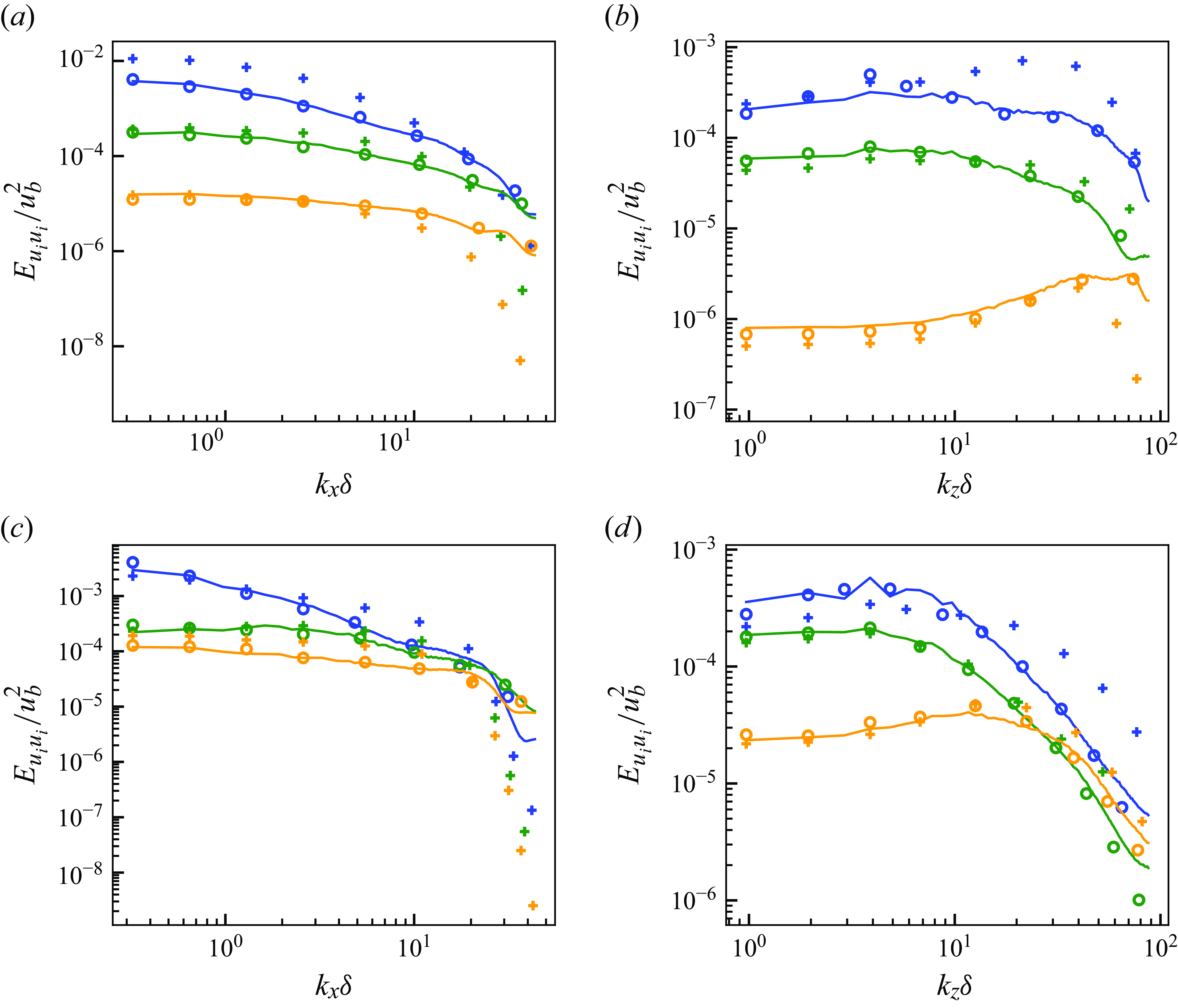
Figure 8. (a,c) Streamwise and (b,d) spanwise energy spectra of predicted velocity for vLES-to-fDNS model $G_{\textit{vLES}-\textit{fDNS}}$
at
$G_{\textit{vLES}-\textit{fDNS}}$
at $Re_\tau \approx 1000$
. Here (a,b)
$Re_\tau \approx 1000$
. Here (a,b) $y^+ \approx 15$
; (c,d)
$y^+ \approx 15$
; (c,d) $y^+ \approx 100$
; blue, streamwise component; orange, wall-normal component; green, spanwise component; solid lines, predicted flow; circles, reference fDNS; pluses, input vLES.
$y^+ \approx 100$
; blue, streamwise component; orange, wall-normal component; green, spanwise component; solid lines, predicted flow; circles, reference fDNS; pluses, input vLES.
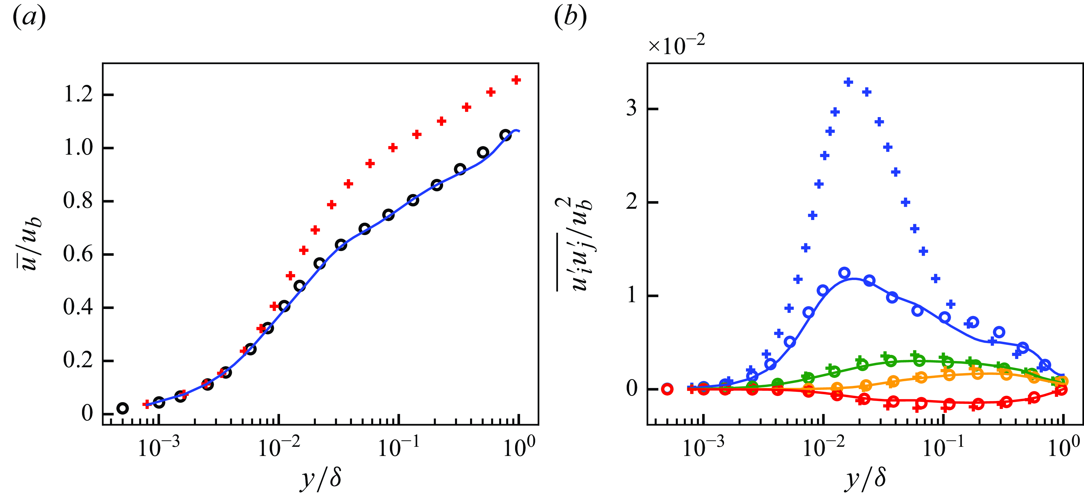
Figure 9. (a) Mean streamwise velocity and (b) resolved reynolds stresses of predicted flow at $Re_\tau \approx 1000$
. Solid lines, predicted flow; circles, reference fDNS; pluses, input vLES. For (b) blue, streamwise normal component (
$Re_\tau \approx 1000$
. Solid lines, predicted flow; circles, reference fDNS; pluses, input vLES. For (b) blue, streamwise normal component ( $\overline {u^{\prime}u^{\prime}}$
); orange, wall-normal normal component (
$\overline {u^{\prime}u^{\prime}}$
); orange, wall-normal normal component ( $\overline {v^{\prime}v^{\prime}}$
); green, spanwise normal component (
$\overline {v^{\prime}v^{\prime}}$
); green, spanwise normal component ( $\overline {w^{\prime}w^{\prime}}$
); red, shear component (
$\overline {w^{\prime}w^{\prime}}$
); red, shear component ( $\overline {u^{\prime}v^{\prime}}$
).
$\overline {u^{\prime}v^{\prime}}$
).
5.1.2. Turbulence spectra and statistics
Figure 8 shows the streamwise and spanwise energy spectra for the three components of velocity at $y^+ \approx 15$
and
$y^+ \approx 15$
and $y^+ \approx 100$
. The input vLES spectra show significant deviations from the fDNS spectra, which show the effects of the insufficient grid resolution of the very coarse computational grid. On the other hand, the predicted output spectra show good agreements with those of the reference fDNS for both off-wall locations shown.
$y^+ \approx 100$
. The input vLES spectra show significant deviations from the fDNS spectra, which show the effects of the insufficient grid resolution of the very coarse computational grid. On the other hand, the predicted output spectra show good agreements with those of the reference fDNS for both off-wall locations shown.
The mean streamwise velocity and the resolved Reynolds stresses of the predicted flows are shown in figure 9. The turbulence statistics show good agreements with those of the reference fDNS. A slight underprediction is observed for the streamwise normal Reynolds stress profiles at $0.1 \lesssim y/\delta \lesssim 0.7$
. Although not shown here, we have confirmed that this discrepancy originates from the underprediction of the low-wavenumber components of turbulence. However, as shown in the later subsections, this discrepancy does not degrade the machine learning pipeline’s ability to predict the correct SGS stresses.
$0.1 \lesssim y/\delta \lesssim 0.7$
. Although not shown here, we have confirmed that this discrepancy originates from the underprediction of the low-wavenumber components of turbulence. However, as shown in the later subsections, this discrepancy does not degrade the machine learning pipeline’s ability to predict the correct SGS stresses.
The results indicate that the unsupervised CycleGAN model is highly effective at converting the non-physical vLES flow fields to physically correct fDNS-quality flow fields. This kind of conversion is impossible without the use of an unsupervised learning method, where paired training data of inputs and expected outputs are not required.

Figure 10. Instantaneous velocity distributions in wall-parallel ( $x$
–
$x$
– $z$
) plane for super-resolution model
$z$
) plane for super-resolution model $G_{\textit{SR}}$
at
$G_{\textit{SR}}$
at $Re_\tau \approx 1000$
. The region corresponds to
$Re_\tau \approx 1000$
. The region corresponds to $(L_x, L_z) = (1.152 \delta , 0.576 \delta )$
. Velocity components are non-dimensionalised by the bulk velocity
$(L_x, L_z) = (1.152 \delta , 0.576 \delta )$
. Velocity components are non-dimensionalised by the bulk velocity $u_b$
. (i,iv,vii) Streamwise component (
$u_b$
. (i,iv,vii) Streamwise component ( $u$
); (ii,v,viii) wall-normal component (
$u$
); (ii,v,viii) wall-normal component ( $v$
); (iii,vi,ix) spanwise component (
$v$
); (iii,vi,ix) spanwise component ( $w$
); (i–iii) input fDNS; (iv–vi) predicted super-resolved flow; (vii–ix) reference DNS.
$w$
); (i–iii) input fDNS; (iv–vi) predicted super-resolved flow; (vii–ix) reference DNS.
5.2. Super-resolution model
$G_{\textit{SR}}$
(cGAN)

This subsection tests the performance of the supervised super-resolution model $G_{\textit{SR}}$
. The model is trained on the paired data of filtered DNS flow fields (fDNS) and the original DNS flow fields, and is designed to super-resolve the fDNS-quality flow fields obtained from
$G_{\textit{SR}}$
. The model is trained on the paired data of filtered DNS flow fields (fDNS) and the original DNS flow fields, and is designed to super-resolve the fDNS-quality flow fields obtained from $G_{\textit{vLES}-\textit{fDNS}}$
in the latter-half of the proposed unsupervised–supervised pipeline. Here, to test the performance of
$G_{\textit{vLES}-\textit{fDNS}}$
in the latter-half of the proposed unsupervised–supervised pipeline. Here, to test the performance of $G_{\textit{SR}}$
individually, the fDNS flow fields obtained from the DNS flow fields are used as the input, and the corresponding DNS flow fields are the references.
$G_{\textit{SR}}$
individually, the fDNS flow fields obtained from the DNS flow fields are used as the input, and the corresponding DNS flow fields are the references.
5.2.1. Instantaneous flow fields
Figure 10 shows the instantaneous velocity distributions of the super-resolved flows from the cGAN model $G_{\textit{SR}}$
. As with figure 6, the wall-normal planes at
$G_{\textit{SR}}$
. As with figure 6, the wall-normal planes at $y^+ \approx 15$
and
$y^+ \approx 15$
and $100$
are shown. Unlike the vLES-to-fDNS model
$100$
are shown. Unlike the vLES-to-fDNS model $G_{\textit{vLES}-\textit{fDNS}}$
which is trained using unsupervised machine learning, this super-resolution model is supervisedly trained since the paired training data of fDNS and DNS can easily be obtained by applying a filter to DNS flow fields. Thus, the reference DNS flow field is the expected instantaneous output for the input fDNS flow field. The figure shows that the super-resolution model can reconstruct the high-wavenumber components that are not present in the input fDNS. Figure 11 shows the streamwise (
$G_{\textit{vLES}-\textit{fDNS}}$
which is trained using unsupervised machine learning, this super-resolution model is supervisedly trained since the paired training data of fDNS and DNS can easily be obtained by applying a filter to DNS flow fields. Thus, the reference DNS flow field is the expected instantaneous output for the input fDNS flow field. The figure shows that the super-resolution model can reconstruct the high-wavenumber components that are not present in the input fDNS. Figure 11 shows the streamwise ( $y$
–
$y$
– $z$
) cross-sectional planes of the velocity fields. As with figure 7, there are no clear discontinuous velocity distributions across the wall-normal direction owing to the similarities between the adjacent wall-normal planes.
$z$
) cross-sectional planes of the velocity fields. As with figure 7, there are no clear discontinuous velocity distributions across the wall-normal direction owing to the similarities between the adjacent wall-normal planes.
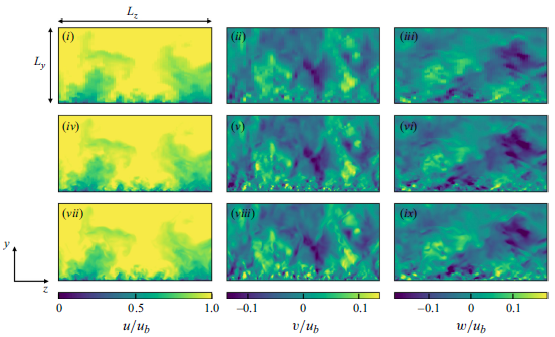
Figure 11. Instantaneous velocity distributions in streamwise ( $y$
–
$y$
– $z$
) cross-sectional plane for super-resolution model
$z$
) cross-sectional plane for super-resolution model $G_{\textit{SR}}$
at
$G_{\textit{SR}}$
at $Re_\tau \approx 1000$
. The region corresponds to
$Re_\tau \approx 1000$
. The region corresponds to $(L_y, L_z) = (\delta , 2 \delta )$
. Velocity components are non-dimensionalised by the bulk velocity
$(L_y, L_z) = (\delta , 2 \delta )$
. Velocity components are non-dimensionalised by the bulk velocity $u_b$
. (i,iv,vii) Streamwise component (
$u_b$
. (i,iv,vii) Streamwise component ( $u$
); (ii,v,viii) wall-normal component (
$u$
); (ii,v,viii) wall-normal component ( $v$
); (iii,vi,ix) spanwise component (
$v$
); (iii,vi,ix) spanwise component ( $w$
); (i–iii) input fDNS; iv–vi) predicted super-resolved flow; (vii–ix) reference DNS.
$w$
); (i–iii) input fDNS; iv–vi) predicted super-resolved flow; (vii–ix) reference DNS.
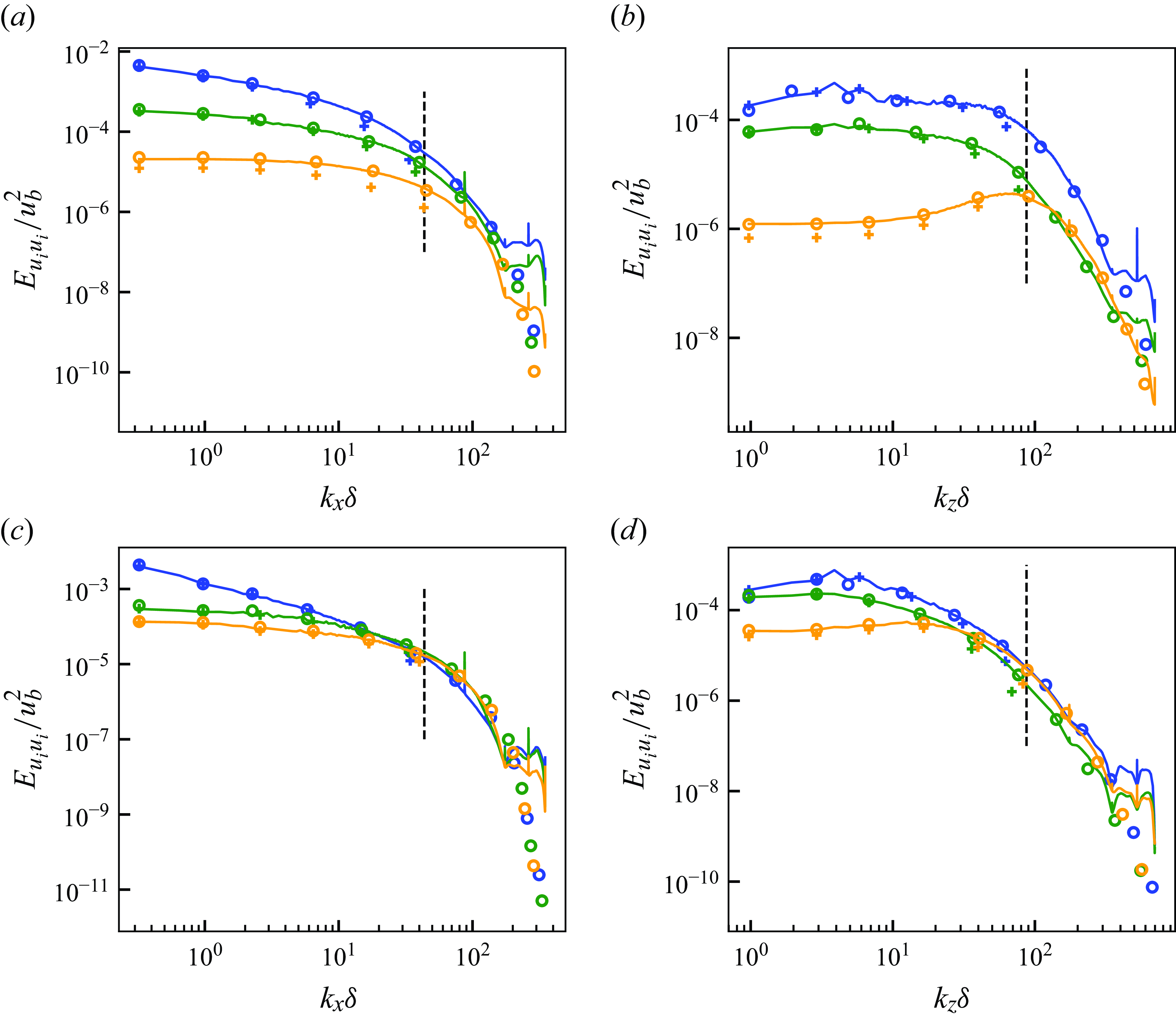
Figure 12. (a,c) Streamwise and (b,d) spanwise energy spectra of predicted super-resolved velocity fields at $Re_\tau \approx 1000$
. Here (a,b)
$Re_\tau \approx 1000$
. Here (a,b) $y^+ \approx 15$
; (c,d)
$y^+ \approx 15$
; (c,d) $y^+ \approx 100$
. Blue, streamwise component; orange, wall-normal component; green, spanwise component. Solid lines, predicted super-resolved flow; circles, reference DNS; pluses, input fDNS. Black vertical dashed lines indicate maximum wavenumber resolved by the input fDNS (cutoff wavenumber).
$y^+ \approx 100$
. Blue, streamwise component; orange, wall-normal component; green, spanwise component. Solid lines, predicted super-resolved flow; circles, reference DNS; pluses, input fDNS. Black vertical dashed lines indicate maximum wavenumber resolved by the input fDNS (cutoff wavenumber).
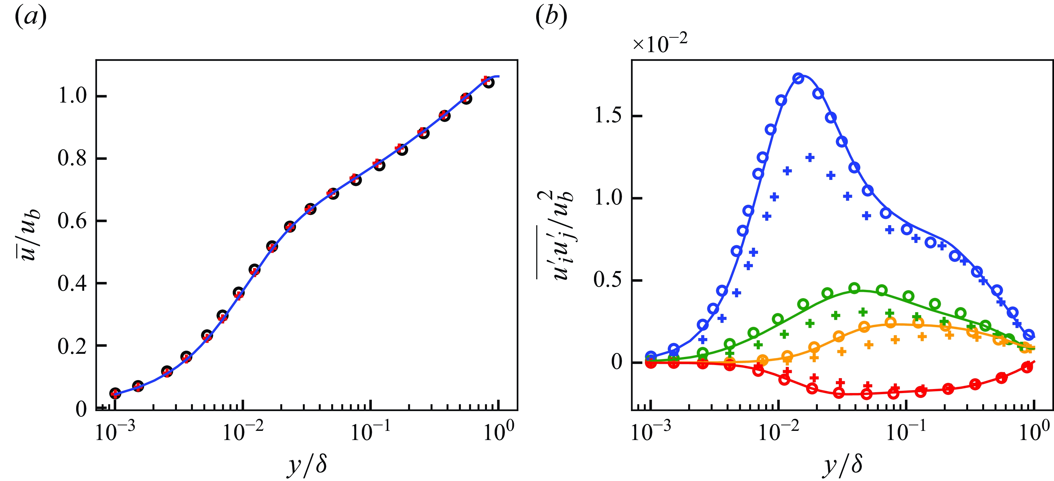
Figure 13. (a) Mean streamwise velocity and (b) resolved Reynolds stresses of predicted super-resolved flows at $Re_\tau \approx 1000$
. Solid lines, predicted super-resolved flow; circles, reference DNS; pluses, input fDNS. For (b) blue, streamwise normal component (
$Re_\tau \approx 1000$
. Solid lines, predicted super-resolved flow; circles, reference DNS; pluses, input fDNS. For (b) blue, streamwise normal component ( $\overline {u^{\prime}u^{\prime}}$
); orange, wall-normal normal component (
$\overline {u^{\prime}u^{\prime}}$
); orange, wall-normal normal component ( $\overline {v^{\prime}v^{\prime}}$
); green, spanwise normal component (
$\overline {v^{\prime}v^{\prime}}$
); green, spanwise normal component ( $\overline {w^{\prime}w^{\prime}}$
); red, shear component (
$\overline {w^{\prime}w^{\prime}}$
); red, shear component ( $\overline {u^{\prime}v^{\prime}}$
).
$\overline {u^{\prime}v^{\prime}}$
).
5.2.2. Turbulence spectra and statistics
In figure 12, the energy spectra of the super-resolved flows are shown. The components of the wavenumbers that are lower than the vertical dashed lines in the figure are resolved by the fDNS, while the higher wavenumber components must be newly generated. In other words, the higher wavenumber components are not included in the input, and they are predicted by the super-resolution model. The predicted flows of the super-resolution model show good agreements in the high-wavenumber components of the flow. While discrepancies are observed in the highest-wavenumber components, they are insignificantly small by three to four orders of magnitude compared with the most energetic eddies. In fact, the discrepancies are indeed negligible to the mean streamwise velocity and the resolved Reynolds stresses, as shown in figure 13. Furthermore, in the resolved wavenumbers (left of the vertical dashed lines), the discrepancies between the input fDNS and the reference DNS are corrected by the super-resolution, most evidently in the wall-normal component. As the low-wavenumber components carry much of the turbulent kinetic energy, this correction is an important part of the super-resolution process in terms of the recovery of the energy. As shown in figure 13, the mean streamwise velocity and the Reynolds stresses of the super-resolved flows show good agreements with those of the reference DNS. We note that the spikes of the spectra occurring at some of the high wavenumbers are known as the chequerboard artefact (Odena, Dumoulin & Olah Reference Odena, Dumoulin and Olah2016). These artefacts are known in the field of computer vision to be avoidable by employing more sophisticated upsampling layers, while the current study uses nearest-neighbour interpolation as shown in Appendix A. However, as the spikes only exist in few wavenumber components and contribute little to the total energy, they pose little problem to the SGS modelling in this study.
5.2.3. Extraction of SGS stresses
The super-resolution model’s ability to predict the SGS stresses is tested in an a priori manner. Figure 14 shows the SGS stresses obtained from the super-resolved DNS-quality flows through the process described in § 3.2. The predicted super-resolved flows agree well with the reference SGS stresses extracted from the original DNS data. Also, the discrepancies in the highest-wavenumbers of the predicted spectra observed in figure 12 do not negatively affect the predicted SGS stresses. The largest energy contained in the unresolved wavenumbers (the energy at the near-cutoff wavenumbers which constitute the majority of the extracted SGS stresses) and the prediction errors near the highest-wavenumbers are separated by around two orders of magnitude, leading to the negligible contribution to the total SGS stress components. The results indicate that the proposed turbulence super-resolution can be used to predict accurate SGS stresses.
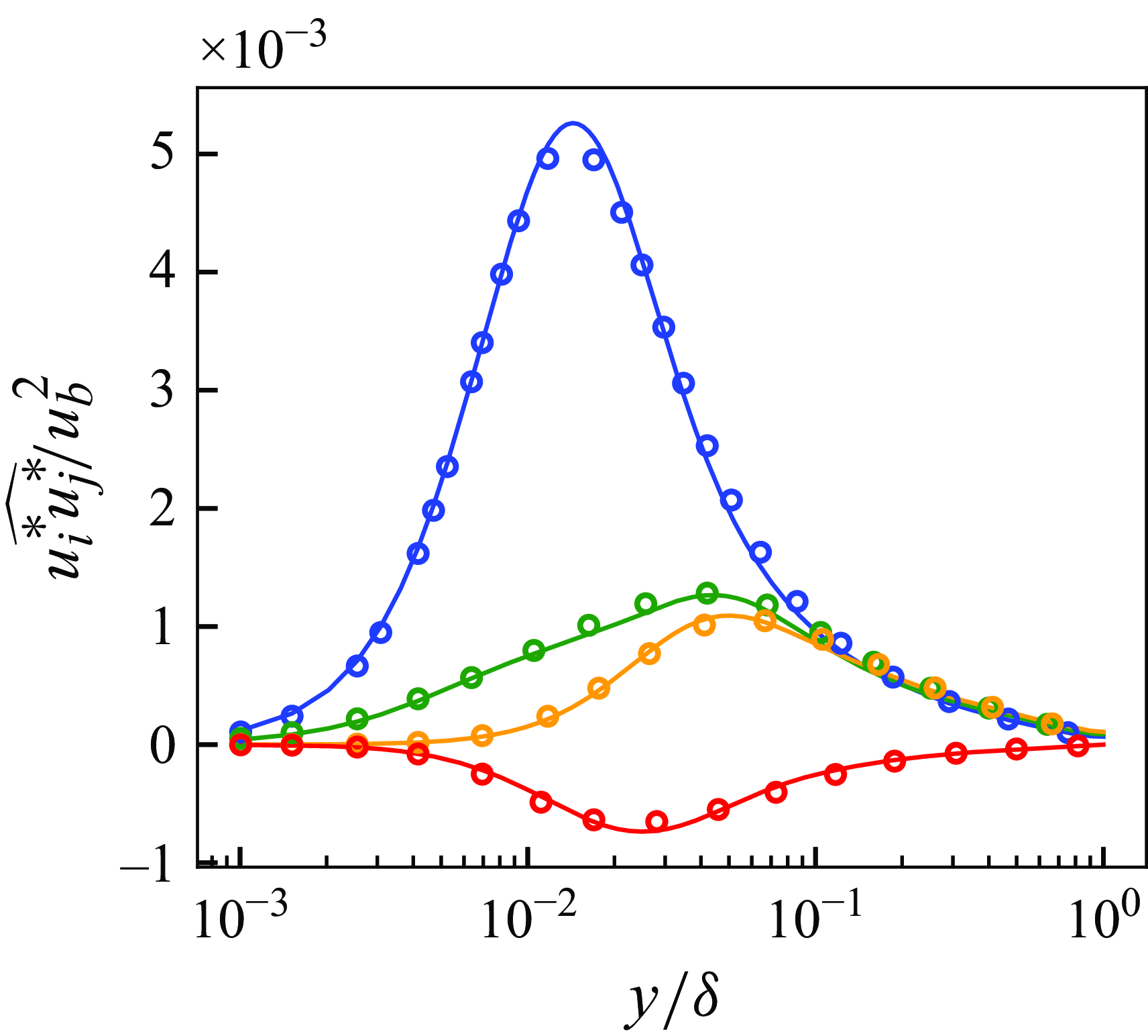
Figure 14. The SGS stresses extracted from flows predicted by the super-resolution model $G_{\textit{SR}}$
at
$G_{\textit{SR}}$
at ${Re}_\tau \approx 1000$
. Solid lines, predicted super-resolved flow; circles, reference DNS. Blue, streamwise normal component (
${Re}_\tau \approx 1000$
. Solid lines, predicted super-resolved flow; circles, reference DNS. Blue, streamwise normal component ( $\widehat {u^* u^*}$
); orange, wall-normal normal component (
$\widehat {u^* u^*}$
); orange, wall-normal normal component ( $\widehat {v^* v^*}$
); green, spanwise normal component (
$\widehat {v^* v^*}$
); green, spanwise normal component ( $\widehat {w^* w^*}$
); red, shear component (
$\widehat {w^* w^*}$
); red, shear component ( $\widehat {u^* v^*}$
).
$\widehat {u^* v^*}$
).
5.3. Entire unsupervised–supervised machine learning pipeline
Finally, the results of the entire unsupervised–supervised machine learning pipeline consisting of the vLES-to-fDNS model $G_{\textit{vLES}-\textit{fDNS}}$
and the super-resolution model
$G_{\textit{vLES}-\textit{fDNS}}$
and the super-resolution model $G_{\textit{SR}}$
, which are obtained by separate trainings as discussed in § 5.1 and § 5.2, are presented. To reiterate, the unsupervised vLES-to-fDNS model
$G_{\textit{SR}}$
, which are obtained by separate trainings as discussed in § 5.1 and § 5.2, are presented. To reiterate, the unsupervised vLES-to-fDNS model $G_{\textit{vLES}-\textit{fDNS}}$
is trained to convert the vLES flow fields to fDNS-quality flow fields (in § 5.1), while the supervised super-resolution model
$G_{\textit{vLES}-\textit{fDNS}}$
is trained to convert the vLES flow fields to fDNS-quality flow fields (in § 5.1), while the supervised super-resolution model $G_{\textit{SR}}$
is trained to convert the fDNS flow fields to DNS-quality flow fields (in § 5.2). The two models form a pipeline in which the fDNS-quality flow fields generated by the vLES-to-fDNS model are input into the super-resolution model to obtain the DNS-quality flow fields. As such, the inputs to the pipeline are the vLES flow fields, and the outputs are the DNS-quality flow fields predicted by the proposed pipeline (figure 3
c). The reference solutions are the DNS flow fields. For comparisons, the results of applying the typical supervised super-resolution model directly to vLES data, which is often used in the super-resolution machine learning community (e.g. Fukami et al. (Reference Fukami, Fukagata and Taira2019)and Obiols-Sales et al. (Reference Obiols-Sales, Vishnu, Malaya and Chandramowlishwaran2021); also see review by Fukami et al. (Reference Fukami, Fukagata and Taira2023)), are also shown to highlight the importance of the unsupervised learning model
$G_{\textit{SR}}$
is trained to convert the fDNS flow fields to DNS-quality flow fields (in § 5.2). The two models form a pipeline in which the fDNS-quality flow fields generated by the vLES-to-fDNS model are input into the super-resolution model to obtain the DNS-quality flow fields. As such, the inputs to the pipeline are the vLES flow fields, and the outputs are the DNS-quality flow fields predicted by the proposed pipeline (figure 3
c). The reference solutions are the DNS flow fields. For comparisons, the results of applying the typical supervised super-resolution model directly to vLES data, which is often used in the super-resolution machine learning community (e.g. Fukami et al. (Reference Fukami, Fukagata and Taira2019)and Obiols-Sales et al. (Reference Obiols-Sales, Vishnu, Malaya and Chandramowlishwaran2021); also see review by Fukami et al. (Reference Fukami, Fukagata and Taira2023)), are also shown to highlight the importance of the unsupervised learning model $G_{\textit{vLES}-\textit{fDNS}}$
in the proposed pipeline. As shown in figure 15, while the proposed pipeline uses the unsupervised vLES-to-fDNS model
$G_{\textit{vLES}-\textit{fDNS}}$
in the proposed pipeline. As shown in figure 15, while the proposed pipeline uses the unsupervised vLES-to-fDNS model $G_{\textit{vLES}-\textit{fDNS}}$
to first convert the vLES flow fields to fDNS-quality flow fields, the typical supervised method applies the super-resolution model directly to the vLES flow fields.
$G_{\textit{vLES}-\textit{fDNS}}$
to first convert the vLES flow fields to fDNS-quality flow fields, the typical supervised method applies the super-resolution model directly to the vLES flow fields.
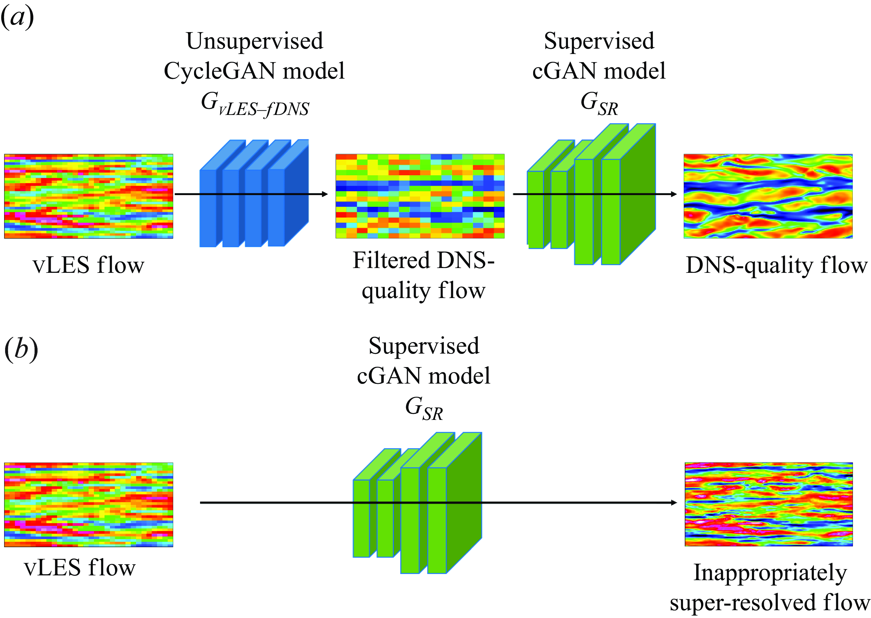
Figure 15. Proposed unsupervised–supervised pipeline architecture (a) compared with typical supervised method (b). In the typical supervised method, the machine learning model trained on fDNS data are used to super-resolve vLES data.
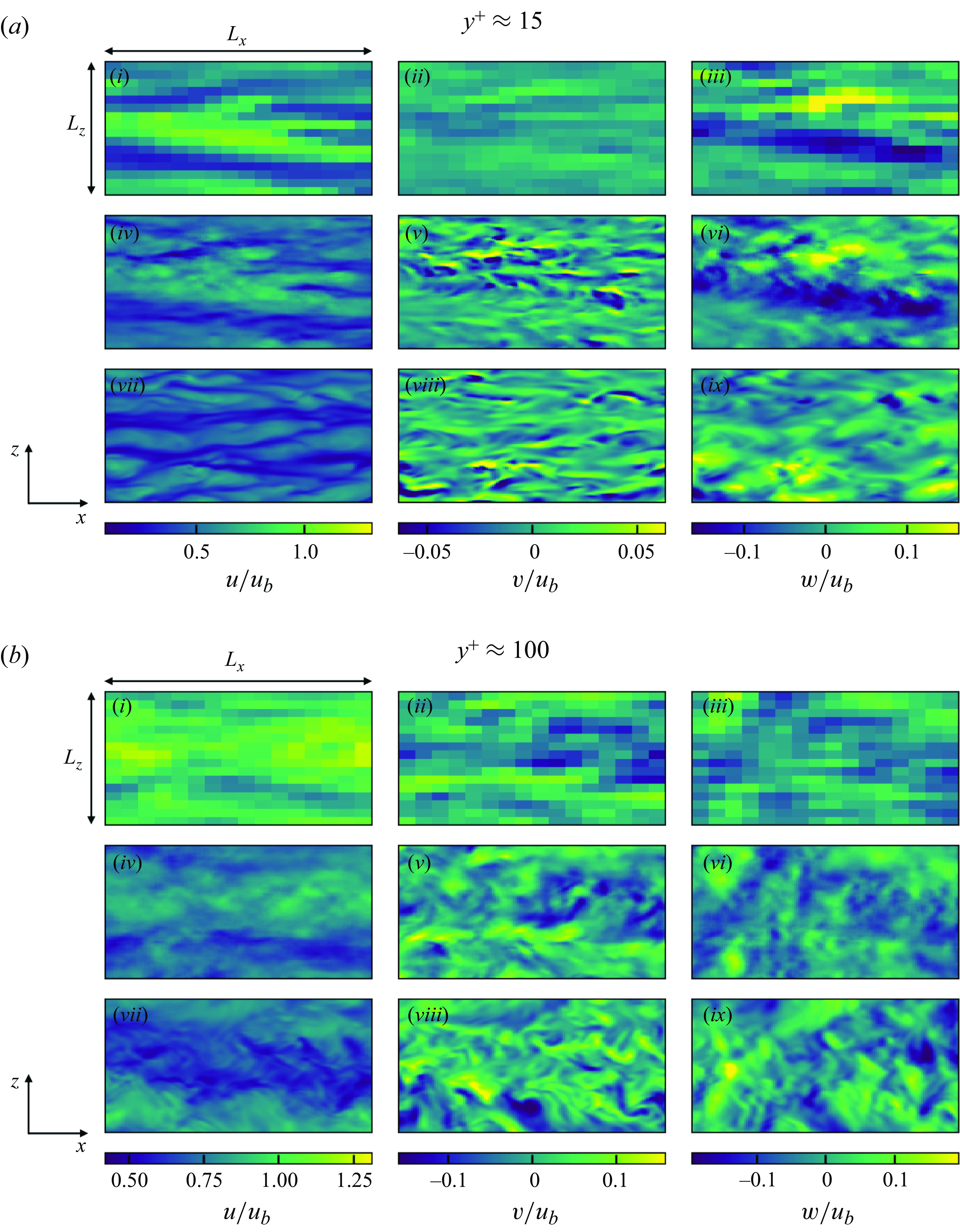
Figure 16. Instantaneous velocity distributions in wall-parallel ( $x$
–
$x$
– $z$
) plane for proposed unsupervised–supervised pipeline at
$z$
) plane for proposed unsupervised–supervised pipeline at ${Re}_\tau \approx 1000$
. The region corresponds to
${Re}_\tau \approx 1000$
. The region corresponds to $(L_x, L_z) = (1.152 \delta , 0.576 \delta )$
. Velocity components are non-dimensionalised by the bulk velocity
$(L_x, L_z) = (1.152 \delta , 0.576 \delta )$
. Velocity components are non-dimensionalised by the bulk velocity $u_b$
. (i,iv,vii) Streamwise component (
$u_b$
. (i,iv,vii) Streamwise component ( $u$
); (ii,v,viii) wall-normal component (
$u$
); (ii,v,viii) wall-normal component ( $v$
); (iii,vi,ix) spanwise component (
$v$
); (iii,vi,ix) spanwise component ( $w$
);(i–iii) input vLES; (iv–vi) predicted super-resolved flow with the proposed pipeline; (vii–ix) reference DNS.
$w$
);(i–iii) input vLES; (iv–vi) predicted super-resolved flow with the proposed pipeline; (vii–ix) reference DNS.
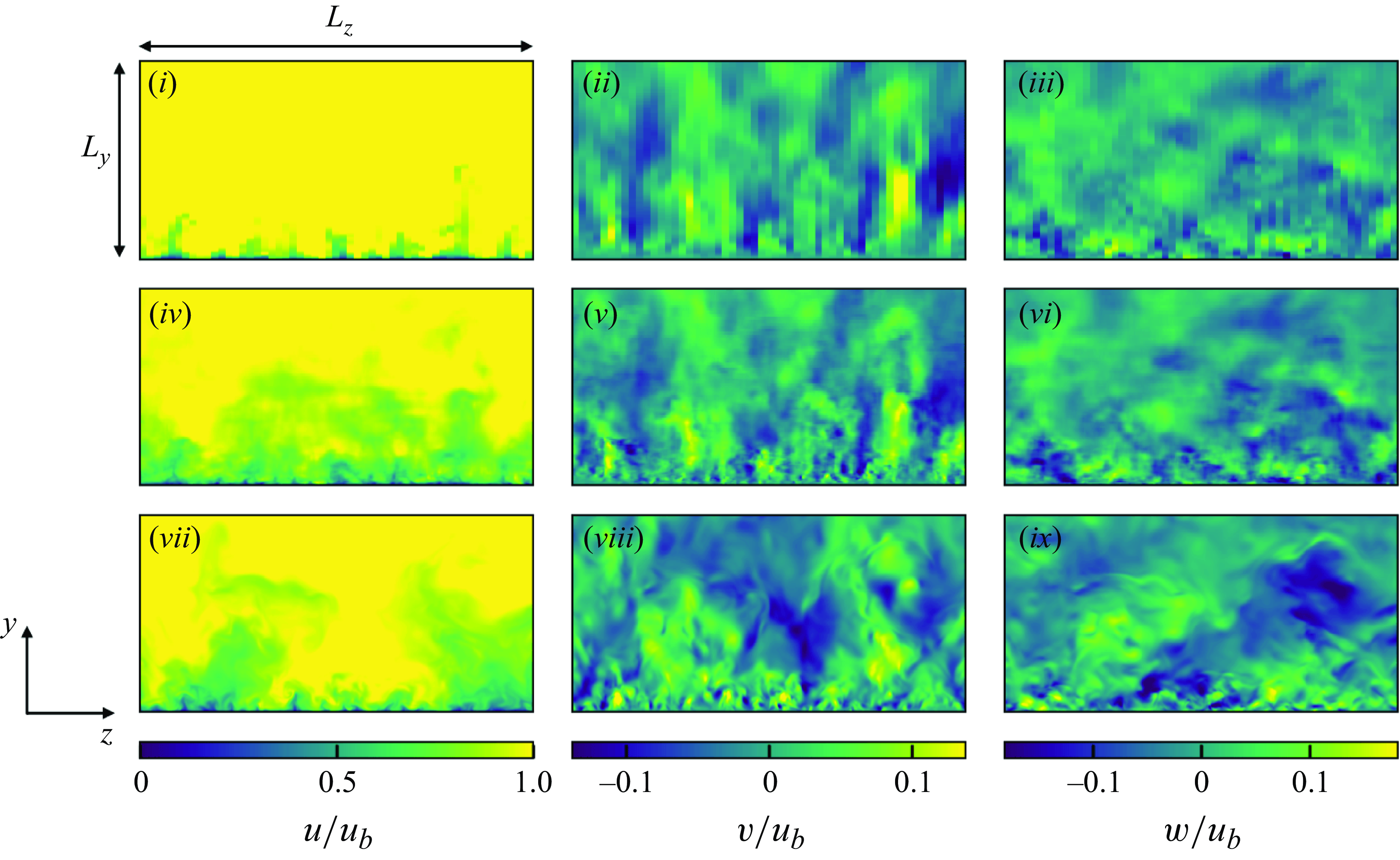
Figure 17. Instantaneous velocity distributions in streamwise ( $y$
–
$y$
– $z$
) plane for proposed unsupervised–supervised pipeline at
$z$
) plane for proposed unsupervised–supervised pipeline at ${Re}_\tau \approx 1000$
. The region corresponds to
${Re}_\tau \approx 1000$
. The region corresponds to $(L_y, L_z) = (\delta , 2 \delta )$
. Velocity components are non-dimensionalised by the bulk velocity
$(L_y, L_z) = (\delta , 2 \delta )$
. Velocity components are non-dimensionalised by the bulk velocity $u_b$
. (i,iv,vii) Streamwise component (
$u_b$
. (i,iv,vii) Streamwise component ( $u$
); (ii,v,viii) wall-normal component (
$u$
); (ii,v,viii) wall-normal component ( $v$
); (iii,vi,ix) spanwise component (
$v$
); (iii,vi,ix) spanwise component ( $w$
); (i–iii) input vLES; (iv–vi) predicted super-resolved flow with the proposed pipeline; (vii–ix) reference DNS.
$w$
); (i–iii) input vLES; (iv–vi) predicted super-resolved flow with the proposed pipeline; (vii–ix) reference DNS.
5.3.1. Instantaneous flow fields
The instantaneous velocity fields of the flows super-resolved by the proposed pipeline are shown in figure 16. We note that the proposed super-resolution machine learning pipeline performs unsupervised super-resolution, and therefore the reference DNS is not exactly the same instantaneous reference solution to the particular instantaneous vLES input as with § 5.1.1. The predicted instantaneous flow fields are expected to show qualitative agreement, such as the turbulent structures and the peak velocity magnitude, and the quantitative assessments will be assessed using turbulence statistics in § 5.3.2. It can be seen from figure 16 that the proposed pipeline successfully decreases the high streamwise velocity at the centre of the domain and successfully generates the stronger fluctuations in the wall-normal velocity, which are the characteristics of the vLES-to-fDNS model discussed in § 5.1.1. Additionally, the predicted distributions show the small-scale turbulent structures similar to the reference DNS that are not present in the input vLES, which is a characteristic of the super-resolution model discussed in § 5.2.1. The predicted velocity distributions suggest that the constructed pipeline exhibits the characteristics of each of the constituents: the vLES-to-fDNS model $G_{\textit{vLES}-\textit{fDNS}}$
and the super-resolution model
$G_{\textit{vLES}-\textit{fDNS}}$
and the super-resolution model $G_{\textit{SR}}$
. It should be noted that this kind of super-resolution is impossible without the use of an unsupervised method such as CycleGAN because it is impossible to obtain the paired flow fields of vLES and DNS required by supervised learning methods. The streamwise (
$G_{\textit{SR}}$
. It should be noted that this kind of super-resolution is impossible without the use of an unsupervised method such as CycleGAN because it is impossible to obtain the paired flow fields of vLES and DNS required by supervised learning methods. The streamwise ( $y$
–
$y$
– $z$
) cross-sectional planes of the velocity fields are shown in figure 17. One may observe that the proposed pipeline predicts the high-wavenumber components qualitatively well, especially near the wall. It can also be seen that the velocity distributions do not present clear discontinuities in the wall-normal direction, similar to figures 7 and 11. As shown in § 5.3.2, the predictions made by the proposed pipeline show quantitative agreements in terms of turbulence spectra and statistics. We also note that the resolved large eddies in the original vLES remain after the super-resolution. This shows that the proposed pipeline successfully creates the DNS-quality flow fields which still contain the large eddies resolved by vLES.
$z$
) cross-sectional planes of the velocity fields are shown in figure 17. One may observe that the proposed pipeline predicts the high-wavenumber components qualitatively well, especially near the wall. It can also be seen that the velocity distributions do not present clear discontinuities in the wall-normal direction, similar to figures 7 and 11. As shown in § 5.3.2, the predictions made by the proposed pipeline show quantitative agreements in terms of turbulence spectra and statistics. We also note that the resolved large eddies in the original vLES remain after the super-resolution. This shows that the proposed pipeline successfully creates the DNS-quality flow fields which still contain the large eddies resolved by vLES.
5.3.2. Turbulence spectra and statistics
Figure 18 shows the energy spectra of the flows super-resolved by the proposed unsupervised–supervised pipeline. The proposed pipeline newly predicts the high-wavenumber components (right of the vertical dashed lines) and corrects the spectra differences in the lower wavenumber range (left of the vertical dashed lines) accurately. As also observed in § 5.2.2, some discrepancies are seen in the highest wavenumber components. These differences, however, are insignificant in the turbulence statistics and the extracted SGS stresses as will be shown in § 5.3.3. The dashed lines show that using only the supervised learning model (as typical flow super-resolution) to super-resolve vLES data does not result in accurate super-resolution. The discrepancy occurs because fDNS flow fields do not have the same turbulence statistics as vLES as discussed in § 1. Therefore, typical supervised learning using fDNS flows as the training data does not learn to properly super-resolve the non-physical vLES flow fields, and thus is not appropriate for application to vLES flow fields. Specifically, in the spanwise premultiplied spectra of the streamwise velocity at $y^+\approx 15$
(although not shown here), the proposed unsupervised–supervised pipeline shows a peak at
$y^+\approx 15$
(although not shown here), the proposed unsupervised–supervised pipeline shows a peak at $k_z \delta \approx 60$
, whereas the typical supervised model shows a peak at
$k_z \delta \approx 60$
, whereas the typical supervised model shows a peak at $k_z \delta \approx 40$
. Converted to wavelengths in wall units, the length scales correspond to
$k_z \delta \approx 40$
. Converted to wavelengths in wall units, the length scales correspond to $\lambda _z^+ \approx 100$
and
$\lambda _z^+ \approx 100$
and $\lambda _z^+ \approx 150$
, respectively. The proposed unsupervised–supervised methodology reproduces the peak at the length scale that corresponds to the well-known streak structures
$\lambda _z^+ \approx 150$
, respectively. The proposed unsupervised–supervised methodology reproduces the peak at the length scale that corresponds to the well-known streak structures $\lambda _z^+ \approx 100$
(Smith & Metzler Reference Smith and Metzler1983), while the typical supervised model produces the peak at the length scale that is approximately 1.5 times longer. These results show the superiority of the proposed unsupervised pipeline method for the super-resolution of the vLES flow fields.
$\lambda _z^+ \approx 100$
(Smith & Metzler Reference Smith and Metzler1983), while the typical supervised model produces the peak at the length scale that is approximately 1.5 times longer. These results show the superiority of the proposed unsupervised pipeline method for the super-resolution of the vLES flow fields.
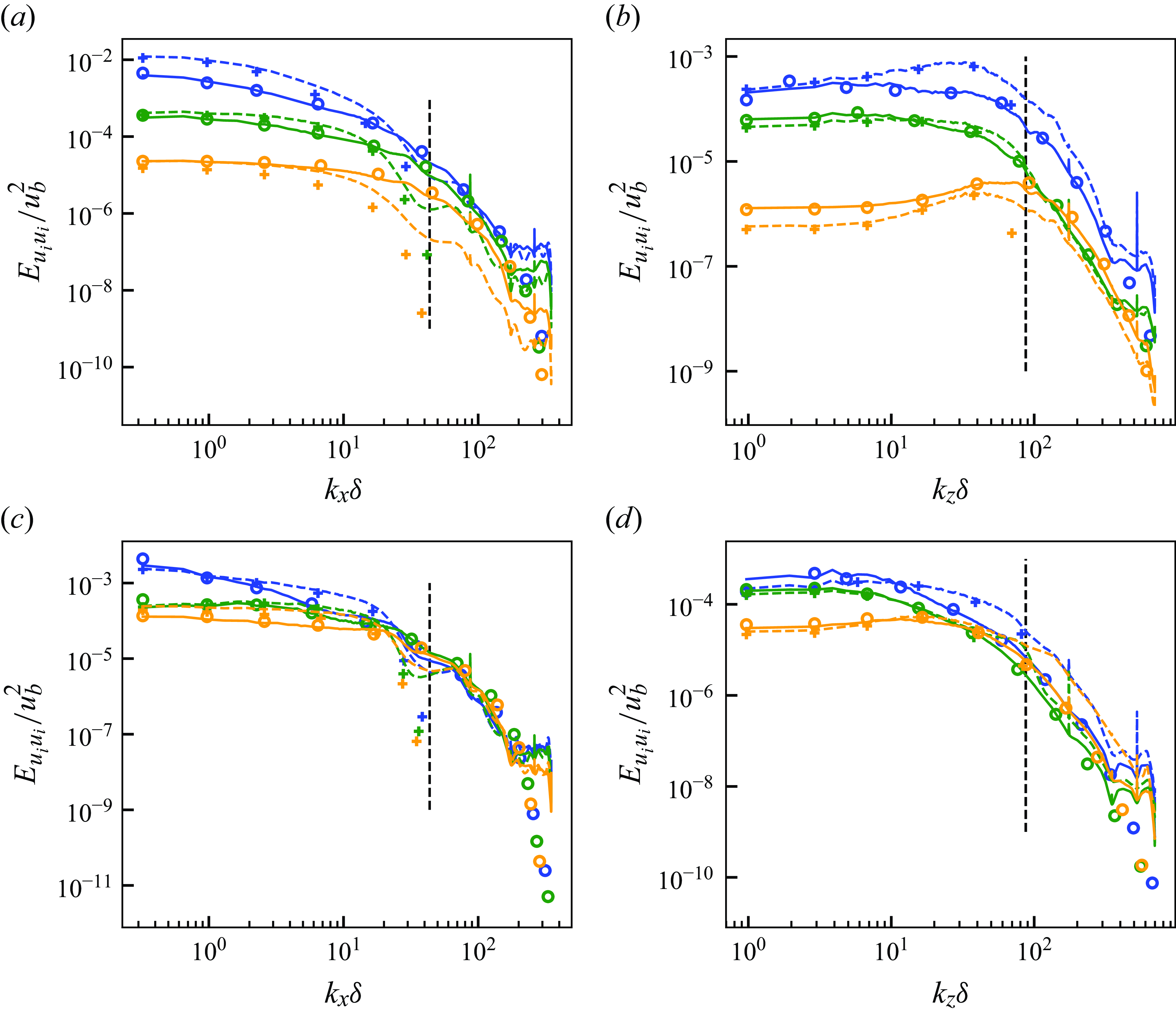
Figure 18. (a,c) Streamwise and (b,d) spanwise energy spectra of predicted super-resolved velocity field with the proposed unsupervised–supervised pipeline at ${Re}_\tau \approx 1000$
. Here (a,b)
${Re}_\tau \approx 1000$
. Here (a,b) $y^+ \approx 15$
; (c,d)
$y^+ \approx 15$
; (c,d) $y^+ \approx 100$
. Blue, streamwise component; orange, wall-normal component; green, spanwise component. Solid lines, predicted super-resolved flow using proposed unsupervised pipeline model (figure 15
a); dashed lines, typical supervised model (figure 15
b); circles, reference DNS; pluses, input vLES. Black vertical dashed lines indicate maximum wavenumber resolved by the input vLES (cutoff wavenumber).
$y^+ \approx 100$
. Blue, streamwise component; orange, wall-normal component; green, spanwise component. Solid lines, predicted super-resolved flow using proposed unsupervised pipeline model (figure 15
a); dashed lines, typical supervised model (figure 15
b); circles, reference DNS; pluses, input vLES. Black vertical dashed lines indicate maximum wavenumber resolved by the input vLES (cutoff wavenumber).
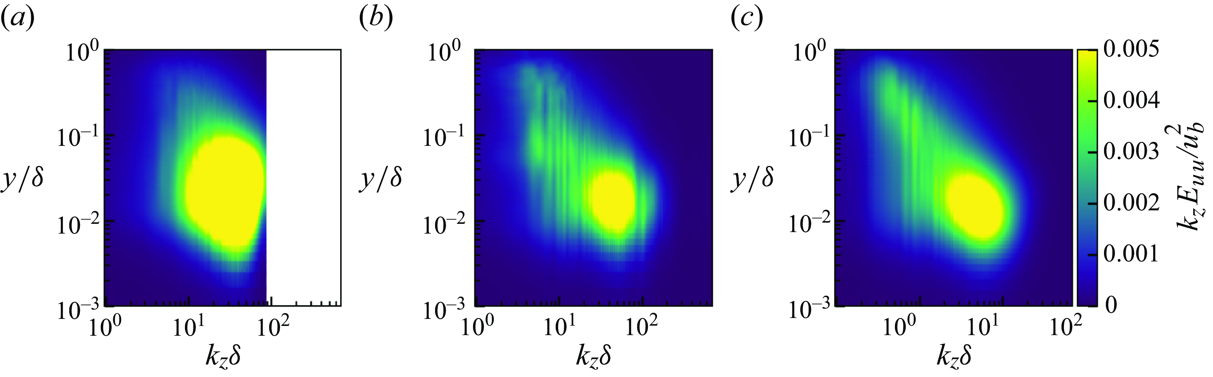
Figure 19. Premultiplied spanwise energy spectra of streamwise velocity for input vLES (a), predicted super-resolved flow using proposed unsupervised–supervised pipeline (b) and reference DNS (c).
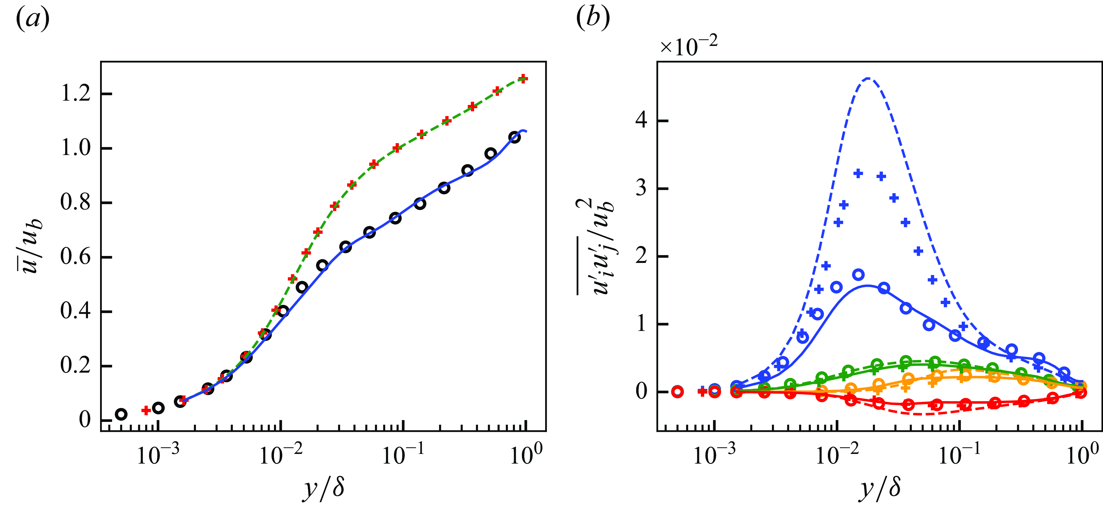
Figure 20. Mean streamwise velocity (a) and resolved Reynolds stresses (b) of predicted super-resolved flows at $Re_\tau \approx 1000$
. Solid lines, predicted super-resolved flow using proposed unsupervised–supervised pipeline (figure 15
a); dashed lines, typical supervised model (figure 15
b); circles, reference DNS; pluses, input vLES. For (b): blue, streamwise normal component (
$Re_\tau \approx 1000$
. Solid lines, predicted super-resolved flow using proposed unsupervised–supervised pipeline (figure 15
a); dashed lines, typical supervised model (figure 15
b); circles, reference DNS; pluses, input vLES. For (b): blue, streamwise normal component ( $\overline {u^{\prime}u^{\prime}}$
); orange, wall-normal normal component (
$\overline {u^{\prime}u^{\prime}}$
); orange, wall-normal normal component ( $\overline {v^{\prime}v^{\prime}}$
); green, spanwise normal component (
$\overline {v^{\prime}v^{\prime}}$
); green, spanwise normal component ( $\overline {w^{\prime}w^{\prime}}$
); red, shear component (
$\overline {w^{\prime}w^{\prime}}$
); red, shear component ( $\overline {u^{\prime}v^{\prime}}$
).
$\overline {u^{\prime}v^{\prime}}$
).
Figure 19 shows the premultiplied spanwise energy spectra of the streamwise velocity for the input vLES, the flow field super-resolved by the proposed pipeline, and the reference DNS. As can be seen from the figure, while the reference DNS shows an increase in energy in the low wavenumber range ( $2 \lesssim k_z \delta \lesssim 10$
) at the outer layer (
$2 \lesssim k_z \delta \lesssim 10$
) at the outer layer ( $y / \delta \gtrsim 0.1$
), the spectra are missing in the input vLES. This energy corresponds to the so-called outer peak (or very large-scale motions) of the turbulent boundary layer in high-Reynolds number flows (Hutchins & Marusic Reference Hutchins and Marusic2007; Marusic et al. Reference Marusic, Mathis and Hutchins2010a
, b; Lee & Moser Reference Lee and Moser2015). The outer peak typically manifests in the spanwise wavelengths of
$y / \delta \gtrsim 0.1$
), the spectra are missing in the input vLES. This energy corresponds to the so-called outer peak (or very large-scale motions) of the turbulent boundary layer in high-Reynolds number flows (Hutchins & Marusic Reference Hutchins and Marusic2007; Marusic et al. Reference Marusic, Mathis and Hutchins2010a
, b; Lee & Moser Reference Lee and Moser2015). The outer peak typically manifests in the spanwise wavelengths of $\lambda _z / \delta \approx 1$
(
$\lambda _z / \delta \approx 1$
( $k_z \delta = 2 \pi \delta / \lambda _z \approx 6$
), as is observed in the present DNS. Furthermore, the outer peak is reported to be missing for wall-modelled LES (Maeyama & Kawai Reference Maeyama and Kawai2023), where the grid resolution with respect to the wall-unit is significantly coarse as is in vLES. On the other hand, the super-resolved flow field shows the presence of the energy in the outer layer, which does not exist in the input vLES data. It can also be seen that the energy peak in the inner-layer (
$k_z \delta = 2 \pi \delta / \lambda _z \approx 6$
), as is observed in the present DNS. Furthermore, the outer peak is reported to be missing for wall-modelled LES (Maeyama & Kawai Reference Maeyama and Kawai2023), where the grid resolution with respect to the wall-unit is significantly coarse as is in vLES. On the other hand, the super-resolved flow field shows the presence of the energy in the outer layer, which does not exist in the input vLES data. It can also be seen that the energy peak in the inner-layer ( $y / \delta \approx 10^{-2}$
) predicted by the proposed pipeline shows better agreement with the reference DNS compared with the vLES. This shows that the proposed unsupervised–supervised machine-learning pipeline not only learns to predict the high-frequency component of turbulence, but also to amend the errors in the low-frequency components that occur in coarse computational grids.
$y / \delta \approx 10^{-2}$
) predicted by the proposed pipeline shows better agreement with the reference DNS compared with the vLES. This shows that the proposed unsupervised–supervised machine-learning pipeline not only learns to predict the high-frequency component of turbulence, but also to amend the errors in the low-frequency components that occur in coarse computational grids.
Figure 20 shows the turbulence statistics of the reconstructed super-resolved flows. The mean streamwise velocity obtained by the proposed pipeline accurately predicts the mean velocity of the reference DNS, whereas the typical supervised super-resolution model, which was supervisedly trained using fDNS flows, yields distributions that do not differ from the input vLES. Similarly, the proposed unsupervised machine learning pipeline can correct the resolved Reynolds stresses and show good agreements with the reference DNS. The super-resolution model alone overestimates the streamwise and shear stresses because of the incorrect mapping learned from fDNS. This likely occurs because the super-resolution model $G_{\textit{SR}}$
is trained merely to predict the small-scale structures missing from the fDNS flow fields, and does not learn to correct the low-frequency components of turbulence. Therefore, the typical supervised model is unable to correct the flow fields that differ from the fDNS flow fields, such as the vLES flow fields. It thus follows that an unsupervisedly trained model is required to perform accurate super-resolution from vLES flow fields, as is proposed in this study.
$G_{\textit{SR}}$
is trained merely to predict the small-scale structures missing from the fDNS flow fields, and does not learn to correct the low-frequency components of turbulence. Therefore, the typical supervised model is unable to correct the flow fields that differ from the fDNS flow fields, such as the vLES flow fields. It thus follows that an unsupervisedly trained model is required to perform accurate super-resolution from vLES flow fields, as is proposed in this study.
5.3.3. Extraction of SGS stresses
Figure 21 shows the SGS stress components extracted from the super-resolved flows with the proposed pipeline using the method described in § 3.2. The SGS stress distributions obtained by the proposed unsupervised–supervised pipeline show good agreements with those from the reference DNS. On the other hand, the super-resolution model based on the typical supervised method overpredicts the magnitude of the SGS stress in the streamwise and shear components. The discrepancies in the predicted SGS stresses are caused by the inappropriate super-resolution performed by the typical supervised model. Additionally, the reference SGS stress components show that the streamwise component is stronger compared with the spanwise and the wall-normal components in the near-wall region, and the proposed pipeline shows good predictions of this relationship. It is also notable that the shear component is well predicted by the proposed pipeline. As the shear stress is directly related to the mean velocity profile through the total shear stress balance within the boundary layer, its accurate prediction is important for the accurate prediction of the mean velocity with vLES.
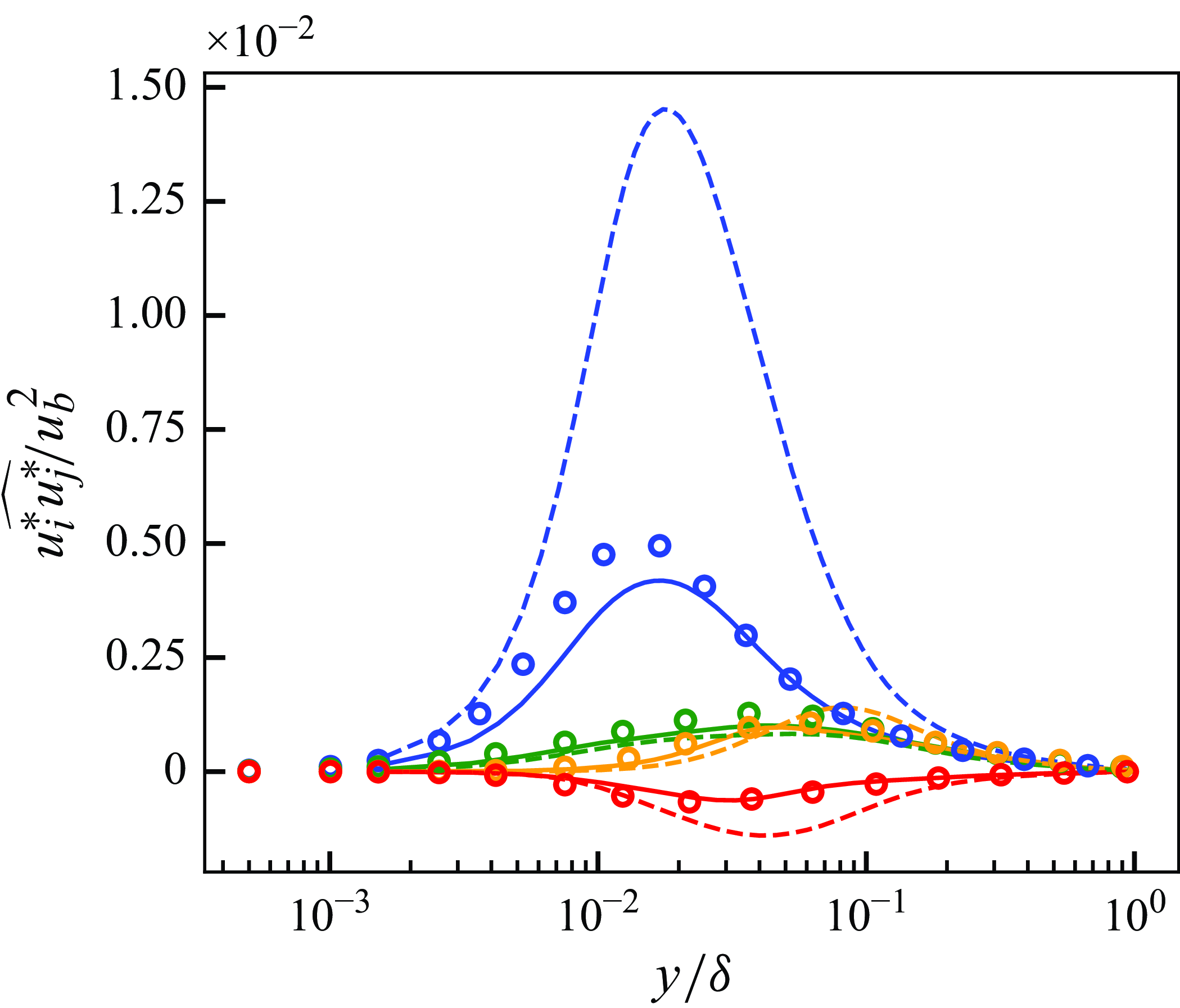
Figure 21. The SGS stresses extracted from predicted super-resolved flows with the proposed unsupervised–supervised pipeline at $Re_\tau \approx 1000$
. Solid lines, predicted super-resolved flow using proposed unsupervised pipeline model (figure 15
a); dashed lines, typical supervised model (figure 15
b); circles, reference DNS. Blue, streamwise normal component (
$Re_\tau \approx 1000$
. Solid lines, predicted super-resolved flow using proposed unsupervised pipeline model (figure 15
a); dashed lines, typical supervised model (figure 15
b); circles, reference DNS. Blue, streamwise normal component ( $\widehat {u^* u^*}$
); orange, wall-normal normal component (
$\widehat {u^* u^*}$
); orange, wall-normal normal component ( $\widehat {v^* v^*}$
); green, spanwise normal component (
$\widehat {v^* v^*}$
); green, spanwise normal component ( $\widehat {w^* w^*}$
); red, shear component (
$\widehat {w^* w^*}$
); red, shear component ( $\widehat {u^* v^*}$
).
$\widehat {u^* v^*}$
).
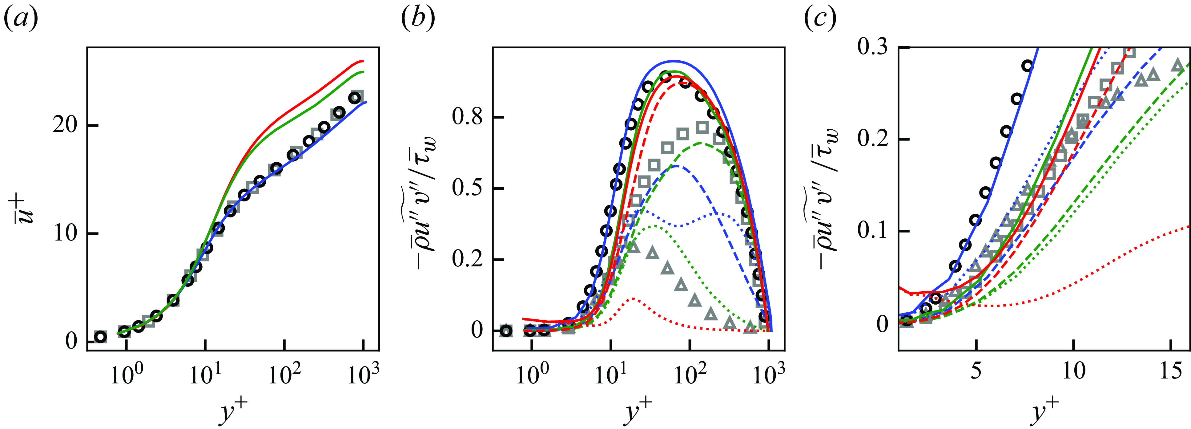
Figure 22. Mean streamwise velocity (a) and Reynolds shear stress (b,c
) of a posteriori tests at $Re_\tau \approx 1000$
. Panel (c) is a near-wall zoomed view of (b). Blue, vLES with proposed unsupervised–supervised-pipeline SGS model (figure 15
a); green, vLES with typical supervised SGS model (figure 15
b); red, vLES with typical SGS model; black circles, reference DNS; grey symbols, reference fDNS. For (b,c): dashed lines and squares, resolved components; dotted lines and triangles, SGS components; solid lines, resolved + SGS components.
$Re_\tau \approx 1000$
. Panel (c) is a near-wall zoomed view of (b). Blue, vLES with proposed unsupervised–supervised-pipeline SGS model (figure 15
a); green, vLES with typical supervised SGS model (figure 15
b); red, vLES with typical SGS model; black circles, reference DNS; grey symbols, reference fDNS. For (b,c): dashed lines and squares, resolved components; dotted lines and triangles, SGS components; solid lines, resolved + SGS components.
6. Very coarse-grid LES with the proposed unsupervised–supervised pipeline SGS model
In this section, the constructed machine-learning-based SGS model is implemented in the LES solver and the vLES is performed using the proposed unsupervised–supervised pipeline SGS model (i.e. the a posteriori test). The constructed model takes the instantaneous velocity distributions $(u,v,w)$
obtained in the vLES and outputs the SGS stress tensor distribution
$(u,v,w)$
obtained in the vLES and outputs the SGS stress tensor distribution $\tau _{\textit{ij}, \textit{SGS}}$
. We emphasise that, as stated in § 1, the primary objective of this study is to obtain an accurate mean streamwise velocity profile on the very coarse grid of vLES. For this purpose, the proposed SGS model must yield the correct profile of the Reynolds shear stress. The predictions of other turbulence statistics, such as the Reynolds normal stresses and higher-order statistics, are not the objective of this study (and should not be expected as will be discussed). However, these statistics are also investigated in this section to clarify their effects on the predicted mean velocity.
$\tau _{\textit{ij}, \textit{SGS}}$
. We emphasise that, as stated in § 1, the primary objective of this study is to obtain an accurate mean streamwise velocity profile on the very coarse grid of vLES. For this purpose, the proposed SGS model must yield the correct profile of the Reynolds shear stress. The predictions of other turbulence statistics, such as the Reynolds normal stresses and higher-order statistics, are not the objective of this study (and should not be expected as will be discussed). However, these statistics are also investigated in this section to clarify their effects on the predicted mean velocity.
The computational set-up is identical to the one used to collect the training data shown in § 4. The results using the conventional SGS model (selective mixed-scale model in this study) and the typical supervised SGS model are also shown for comparisons. As with § 5, the results for the LESx8 case are shown in this section and are referred to as vLES. As shown in Appendix B, the proposed methodology also performs well for the LESx4 case without major drawbacks.
6.1. Overview of the obtained results
Figure 22 shows the obtained mean streamwise velocity and the Reynolds shear stress of the a posteriori tests. The results are compared with the DNS results and the fDNS results obtained from top-hat filtered DNS results. We note that due to the very coarse grid employed by the vLES and the related discretisation errors, it is debatable that the resolved and SGS shear stresses should match the fDNS data quantitatively. Therefore, we believe that the values of the resolved and SGS components from the vLES should not be compared directly with the fDNS data. On the other hand, the total shear stress can be compared quantitatively as its accurate prediction is required to obtain the correct mean streamwise velocity profile, which is the main focus of this study. As discussed in § 4.1, the typical SGS model significantly overpredicts the mean streamwise velocity as shown in figure 22(a). Contrarily, the proposed unsupervised–supervised-pipeline SGS model shows good agreement with the reference DNS. While the typical supervised SGS model shows a slightly better prediction compared with the typical SGS model, the obtained velocity is still overpredicted. The Reynolds shear stress (figure 22
b) shows that the proposed unsupervised–supervised-pipeline SGS model shows good agreements of the total shear stress (solid lines in figure) with the reference DNS, especially for the rise of the Reynolds shear stress in the near-wall region ( $3 \lesssim y^+ \lesssim 30$
). It can also be seen qualitatively within the near-wall region that the SGS shear stress predicted by the proposed SGS model exceeds the resolved shear stress and contributes significantly to the rise of the Reynolds shear stress, which is in agreement with the fDNS results at
$3 \lesssim y^+ \lesssim 30$
). It can also be seen qualitatively within the near-wall region that the SGS shear stress predicted by the proposed SGS model exceeds the resolved shear stress and contributes significantly to the rise of the Reynolds shear stress, which is in agreement with the fDNS results at $3 \lesssim y^+ \lesssim 10$
(zoomed-in view in figure 22
c). On the other hand, the prediction by the typical SGS model shows that the predicted SGS shear stress is smaller than the resolved component, and the total shear stress is underpredicted.
$3 \lesssim y^+ \lesssim 10$
(zoomed-in view in figure 22
c). On the other hand, the prediction by the typical SGS model shows that the predicted SGS shear stress is smaller than the resolved component, and the total shear stress is underpredicted.
The mean streamwise velocity profile and the Reynolds shear stress are closely related through the total shear stress balance of the turbulent channel, which reads
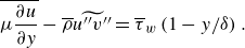 \begin{equation} \overline { \mu \frac {\partial {u}}{\partial y}} - \overline {\rho } \widetilde {u^{\prime\prime} v^{\prime\prime}} = \overline {\tau }_w \left ( 1 - y / \delta \right ). \end{equation}
This equation states that at the off-wall distance $y$
, the sum of the viscous shear stress
$y$
, the sum of the viscous shear stress $\overline { \mu ({\partial {u}}/{\partial x})}$
and the Reynolds shear stress
$\overline { \mu ({\partial {u}}/{\partial x})}$
and the Reynolds shear stress $- \overline {\rho } \widetilde {u^{\prime\prime}v^{\prime\prime}}$
is a constant
$- \overline {\rho } \widetilde {u^{\prime\prime}v^{\prime\prime}}$
is a constant $\overline {\tau }_w ( 1 - y/\delta )$
. In the present vLES, because the proposed unsupervised–supervised-pipeline SGS model is able to accurately predict the near-wall Reynolds shear stress, the viscous shear stress is also accurately predicted. As the viscous stress is proportional to the velocity gradient
$\overline {\tau }_w ( 1 - y/\delta )$
. In the present vLES, because the proposed unsupervised–supervised-pipeline SGS model is able to accurately predict the near-wall Reynolds shear stress, the viscous shear stress is also accurately predicted. As the viscous stress is proportional to the velocity gradient $\partial {u} / \partial y$
, this results in the accurate prediction of the mean velocity. On the other hand, both the conventional SGS model and the conventional supervised SGS model underpredict the Reynolds shear stress in the near-wall region. As a result, the viscous stress is overpredicted which leads to the overprediction of the velocity. In particular, it can be seen that the predicted streamwise velocity profile is sensitive to the prediction accuracy of the near-wall Reynolds shear stress, suggesting the importance of the near-wall prediction accuracies of the Reynolds shear stress.
$\partial {u} / \partial y$
, this results in the accurate prediction of the mean velocity. On the other hand, both the conventional SGS model and the conventional supervised SGS model underpredict the Reynolds shear stress in the near-wall region. As a result, the viscous stress is overpredicted which leads to the overprediction of the velocity. In particular, it can be seen that the predicted streamwise velocity profile is sensitive to the prediction accuracy of the near-wall Reynolds shear stress, suggesting the importance of the near-wall prediction accuracies of the Reynolds shear stress.
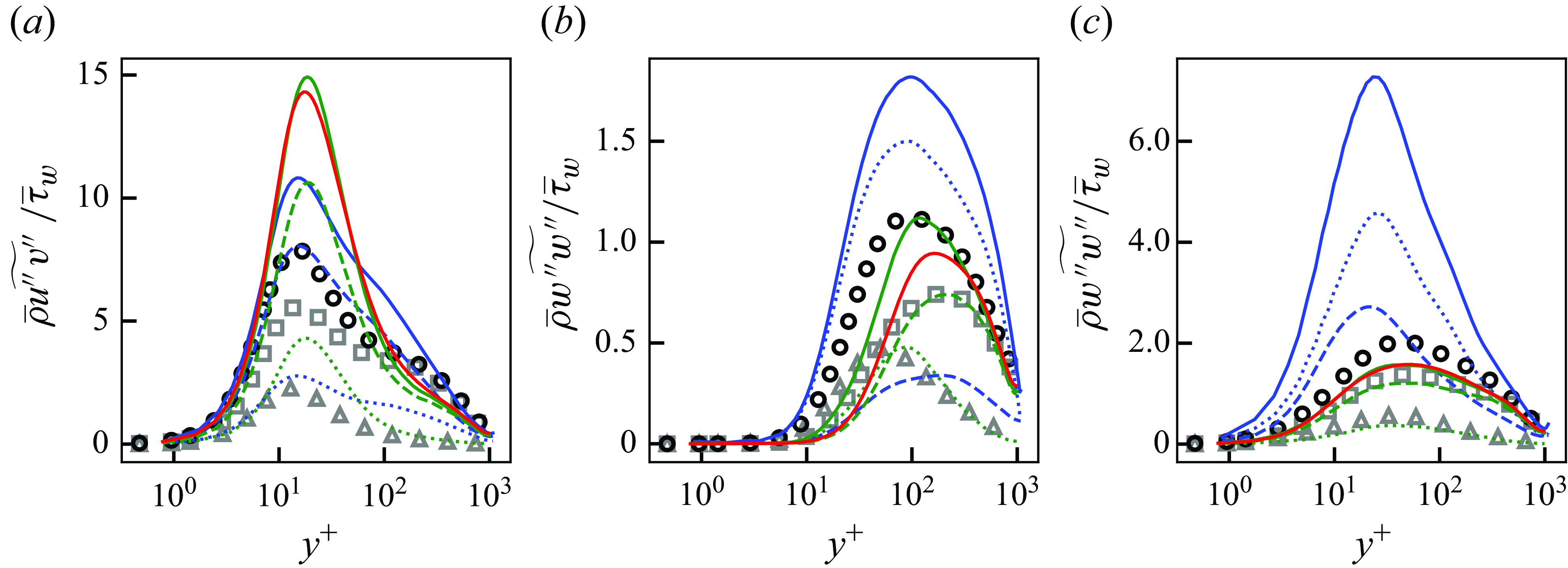
Figure 23. Streamwise (a), wall-normal (b) and spanwise (c) Reynolds stresses of a posteriori tests at $Re_\tau \approx 1000$
. Blue, vLES with proposed unsupervised SGS model (figure 15
a); green, vLES with typical supervised SGS model (figure 15
b); red, vLES with typical SGS model; black circles, reference DNS; grey symbols, reference fDNS. Dashed lines and squares, resolved components; dotted lines and triangles, SGS components; solid lines, resolved + SGS components.
$Re_\tau \approx 1000$
. Blue, vLES with proposed unsupervised SGS model (figure 15
a); green, vLES with typical supervised SGS model (figure 15
b); red, vLES with typical SGS model; black circles, reference DNS; grey symbols, reference fDNS. Dashed lines and squares, resolved components; dotted lines and triangles, SGS components; solid lines, resolved + SGS components.
We note that because we employ the constant body force condition to drive the channel flow as discussed in § 4.1, the predicted mass flow rates vary between the computational cases. Specifically, the mass flow rate obtained by the typical SGS model is overpredicted by $23\,\%$
compared with the DNS, while the proposed machine-learning-based SGS model improves the prediction to a
$23\,\%$
compared with the DNS, while the proposed machine-learning-based SGS model improves the prediction to a $10\,\%$
overprediction. Since the error of the mass flow rate under the constant body force condition is smaller for the proposed SGS machine-learning-based model compared with the typical SGS model, it is expected that the proposed SGS model yields a better prediction of the wall shear stress under the constant mass flow rate condition.
$10\,\%$
overprediction. Since the error of the mass flow rate under the constant body force condition is smaller for the proposed SGS machine-learning-based model compared with the typical SGS model, it is expected that the proposed SGS model yields a better prediction of the wall shear stress under the constant mass flow rate condition.
To investigate the origin of the differences in the Reynolds shear stress, the profiles of the three components of the Reynolds normal stresses are shown in figure 23. In the near-wall region ( $y^+ \lesssim 10$
), similar profiles are predicted in the streamwise component amongst the SGS models, while the wall-normal and spanwise components shows discrepancies with the proposed unsupervised–supervised-pipeline SGS model predicting a near-wall increase of the Reynolds normal stresses
$y^+ \lesssim 10$
), similar profiles are predicted in the streamwise component amongst the SGS models, while the wall-normal and spanwise components shows discrepancies with the proposed unsupervised–supervised-pipeline SGS model predicting a near-wall increase of the Reynolds normal stresses $\overline {\rho } \widetilde {v^{\prime\prime} v^{\prime\prime}}$
and
$\overline {\rho } \widetilde {v^{\prime\prime} v^{\prime\prime}}$
and $\overline {\rho } \widetilde {w^{\prime\prime} w^{\prime\prime}}$
. Another observation is that, in the wall-normal and spanwise components for the proposed unsupervised–supervised-pipeline SGS model, a larger fraction of the total stress comes from the predicted SGS stresses. The wall-normal component for the fDNS also exhibit larger SGS stress than the resolved stress in the near-wall region. These trends are similar to the Reynolds shear stress presented in figure 22. Considering that the Reynolds shear stress is written as the covariance between the streamwise and the wall-normal velocity fluctuations, the differences in the near-wall Reynolds shear stresses (and thus the velocity profiles) between the SGS models are considered to be originated from the differences in the near-wall wall-normal Reynolds stresses.
$\overline {\rho } \widetilde {w^{\prime\prime} w^{\prime\prime}}$
. Another observation is that, in the wall-normal and spanwise components for the proposed unsupervised–supervised-pipeline SGS model, a larger fraction of the total stress comes from the predicted SGS stresses. The wall-normal component for the fDNS also exhibit larger SGS stress than the resolved stress in the near-wall region. These trends are similar to the Reynolds shear stress presented in figure 22. Considering that the Reynolds shear stress is written as the covariance between the streamwise and the wall-normal velocity fluctuations, the differences in the near-wall Reynolds shear stresses (and thus the velocity profiles) between the SGS models are considered to be originated from the differences in the near-wall wall-normal Reynolds stresses.
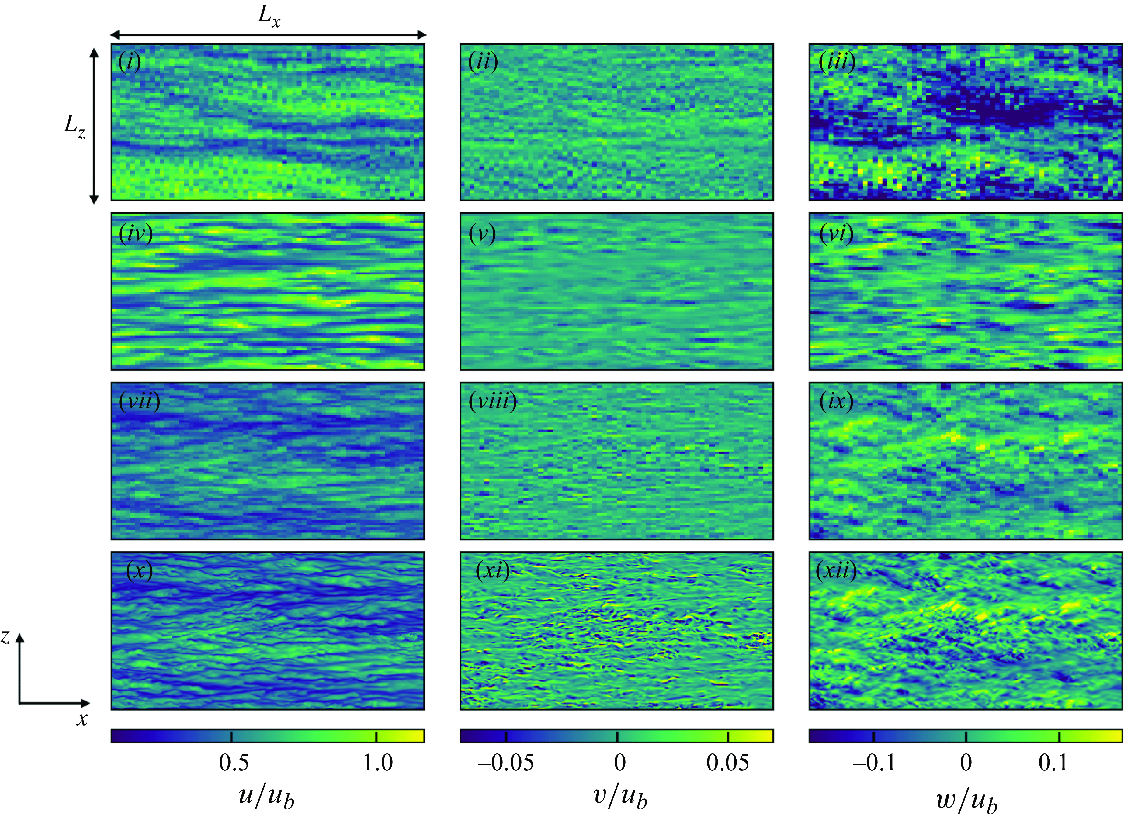
Figure 24. Instantaneous velocity distributions of a posteriori tests at $y^+ \approx 15$
at
$y^+ \approx 15$
at $Re_\tau \approx 1000$
. The region corresponds to
$Re_\tau \approx 1000$
. The region corresponds to $(L_x, L_z) = (4.608 \delta , 2.304 \delta )$
. Velocity components are non-dimensionalised by the bulk velocity
$(L_x, L_z) = (4.608 \delta , 2.304 \delta )$
. Velocity components are non-dimensionalised by the bulk velocity $u_b$
. (i,iv,vii,x) Streamwise component (
$u_b$
. (i,iv,vii,x) Streamwise component ( $u$
); (ii,v,viii,xi) wall-normal component (
$u$
); (ii,v,viii,xi) wall-normal component ( $v$
); (iii,vi,ix,xii) spanwise component (
$v$
); (iii,vi,ix,xii) spanwise component ( $w$
); (i–iii) vLES with proposed unsupervised SGS model; (iv–vi) vLES with typical SGS model; (vii–ix) reference fDNS; (x–xii) reference DNS.
$w$
); (i–iii) vLES with proposed unsupervised SGS model; (iv–vi) vLES with typical SGS model; (vii–ix) reference fDNS; (x–xii) reference DNS.
To clarify the differences in the near-wall Reynolds normal stresses, the instantaneous velocity distributions of the a posteriori tests at $y^+ \approx 15$
are presented in figure 24. The figure also shows the fDNS flow field, which is in concept the reference flow field of vLES. Compared with the reference DNS and fDNS, the typical SGS model non-physically enlarges and deforms the near-wall resolved turbulent structures. In can also be seen that the amplitude of the streamwise velocity fluctuations is larger while that for the wall-normal velocity is smaller. In comparison, the proposed unsupervised–supervised-pipeline SGS model shows fine turbulent structures in the resolved flow field that show resemblance to DNS. Importantly, the proposed model creates the small-scale structures in the wall-normal velocity distributions that are observed for the DNS but not for the typical SGS model. These differences in the resolved turbulence are considered to be the cause of the differences in the near-wall wall-normal Reynolds stresses between the SGS models observed in figure 23. It is also noteworthy that the spanwise velocity magnitudes are larger in the proposed unsupervised–supervised-pipeline SGS model compared with the typical SGS model and the DNS, corresponding to the large near-wall spanwise Reynolds stress.
$y^+ \approx 15$
are presented in figure 24. The figure also shows the fDNS flow field, which is in concept the reference flow field of vLES. Compared with the reference DNS and fDNS, the typical SGS model non-physically enlarges and deforms the near-wall resolved turbulent structures. In can also be seen that the amplitude of the streamwise velocity fluctuations is larger while that for the wall-normal velocity is smaller. In comparison, the proposed unsupervised–supervised-pipeline SGS model shows fine turbulent structures in the resolved flow field that show resemblance to DNS. Importantly, the proposed model creates the small-scale structures in the wall-normal velocity distributions that are observed for the DNS but not for the typical SGS model. These differences in the resolved turbulence are considered to be the cause of the differences in the near-wall wall-normal Reynolds stresses between the SGS models observed in figure 23. It is also noteworthy that the spanwise velocity magnitudes are larger in the proposed unsupervised–supervised-pipeline SGS model compared with the typical SGS model and the DNS, corresponding to the large near-wall spanwise Reynolds stress.
From these results, we can observe that the proposed unsupervised–supervised-pipeline SGS model enables better predictions of the mean streamwise velocity and the Reynolds shear stress, and the use of the unsupervised vLES-to-fDNS model $G_{\textit{vLES}-\textit{fDNS}}$
significantly contributes to the quality of the predictions. The results indicate that the differences in the mean streamwise velocity and the Reynolds shear stress are caused by the differences in the near-wall wall-normal component of the Reynolds stress. Here, we stress again that accurately predicting the Reynolds shear stress and the resultant mean streamwise velocity profile is the primary objective of vLES. The overpredicted wall-normal and spanwise Reynolds stresses observed in figure 23, while non-physical, enable this objective as will be shown in § 6.2.1. In the following, we conduct the budget analyses of the Reynolds stresses to investigate how the near-wall Reynolds shear stress correctly rises leading to the accurate mean velocity profile despite the very coarse grid resolution for the near-wall turbulence structures. Moreover, we investigate the turbulence mechanisms behind the rise of the near-wall wall-normal Reynolds stress which is considered to be the primary origin of the accurately predicted near-wall Reynolds shear stress.
$G_{\textit{vLES}-\textit{fDNS}}$
significantly contributes to the quality of the predictions. The results indicate that the differences in the mean streamwise velocity and the Reynolds shear stress are caused by the differences in the near-wall wall-normal component of the Reynolds stress. Here, we stress again that accurately predicting the Reynolds shear stress and the resultant mean streamwise velocity profile is the primary objective of vLES. The overpredicted wall-normal and spanwise Reynolds stresses observed in figure 23, while non-physical, enable this objective as will be shown in § 6.2.1. In the following, we conduct the budget analyses of the Reynolds stresses to investigate how the near-wall Reynolds shear stress correctly rises leading to the accurate mean velocity profile despite the very coarse grid resolution for the near-wall turbulence structures. Moreover, we investigate the turbulence mechanisms behind the rise of the near-wall wall-normal Reynolds stress which is considered to be the primary origin of the accurately predicted near-wall Reynolds shear stress.
6.2. Analysis of Reynolds stress budget
In this subsection, we discuss the turbulence mechanism that leads to the correct rise of the near-wall wall-normal Reynolds stress (and thus the correct near-wall Reynolds shear stress) despite the insufficient grid resolution of vLES through the budget analyses of the Reynolds stress components. As the flow is at the low Mach number of $M_b \approx 0.1$
, the following analyses are performed with the incompressible assumption. Therefore, we assume that the Favre-averaged velocity
$M_b \approx 0.1$
, the following analyses are performed with the incompressible assumption. Therefore, we assume that the Favre-averaged velocity $\widetilde {u}_i$
approximately equals the Reynolds-averaged velocity
$\widetilde {u}_i$
approximately equals the Reynolds-averaged velocity $\overline {u}_i$
, and that the Reynolds stress in the previous subsection
$\overline {u}_i$
, and that the Reynolds stress in the previous subsection $\overline {\rho } \widetilde {u^{\prime\prime}_i u^{\prime\prime}_j}$
approximately equals
$\overline {\rho } \widetilde {u^{\prime\prime}_i u^{\prime\prime}_j}$
approximately equals $\overline {\rho u^{\prime}_i u^{\prime}_j}$
. This assumption is confirmed to hold well for the present computations.
$\overline {\rho u^{\prime}_i u^{\prime}_j}$
. This assumption is confirmed to hold well for the present computations.
6.2.1. Effect of SGS stresses on near-wall Reynolds stresses
As discussed in § 1, this study aims to obtain the accurate prediction of the mean velocity (first-order statistics) and the closely related Reynolds shear stress (second-order statistics) from the vLES. Therefore, the agreement of the Reynolds stress budgets (third-order statistics) between the proposed SGS model and the reference DNS is not the goal of this study. Rather, we focus on understanding the mechanism that lead to the accurate predictions of the mean streamwise velocity and the Reynolds shear stress obtained by the proposed unsupervised–supervised-pipeline SGS model. We also note that the following analyses reveal that the DNS-obtained Reynolds normal stresses and the budgets should not be expected in the vLES to obtain the correct mean velocity and Reynolds shear stress.
The budget equation of the resolved Reynolds stresses is given as follows:
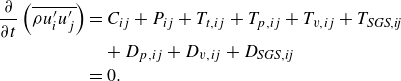 \begin{align} \frac {\partial }{\partial t} \left ( \overline {\rho u^{\prime}_i u^{\prime}_j} \right ) & = C_{ij} + P_{ij} + T_{t,ij} + T_{p,ij} + T_{v,ij} + T_{\textit{SGS},\textit{ij}} \nonumber \\ & \quad + D_{p,ij} + D_{v,ij} + D_{\textit{SGS},\textit{ij}} \nonumber \\ &= 0. \end{align}
Here, the subscripts $i,j = (1,2,3)$
denote the streamwise, wall-normal and spanwise directions respectively, and
$i,j = (1,2,3)$
denote the streamwise, wall-normal and spanwise directions respectively, and
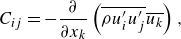 \begin{align}&\qquad\qquad C_{ij} = - \frac {\partial }{\partial x_k} \left ( \overline {\rho u^{\prime}_i u^{\prime}_j} \overline {u_k} \right ), \end{align}
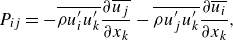 \begin{align}&\qquad P_{ij} = - \overline {\rho u^{\prime}_i u^{\prime}_k} \frac {\partial \overline {u_j}}{\partial x_k} - \overline {\rho u^{\prime}_j u^{\prime}_k} \frac {\partial \overline {u_i}}{\partial x_k}, \end{align}
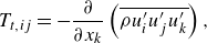 \begin{align}&\qquad\qquad T_{t,ij} = - \frac {\partial }{\partial x_k} \left ( \overline {\rho u^{\prime}_i u^{\prime}_j u^{\prime}_k} \right ), \end{align}
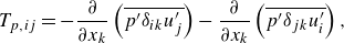 \begin{align}&\quad T_{p,ij} = - \frac {\partial }{\partial x_k} \left ( \overline {p^{\prime} \delta _{ik} u^{\prime}_j} \right ) - \frac {\partial }{\partial x_k} \left ( \overline {p^{\prime} \delta _{jk} u^{\prime}_i} \right ), \end{align}
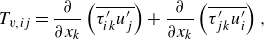 \begin{align}&\qquad T_{v,ij} = \frac {\partial }{\partial x_k} \left ( \overline {\tau ^{\prime}_{ik} u^{\prime}_j} \right ) + \frac {\partial }{\partial x_k} \left ( \overline {\tau ^{\prime}_{jk} u^{\prime}_i} \right ), \end{align}
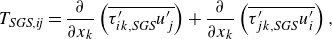 \begin{align}& T_{\textit{SGS},\textit{ij}} = \frac {\partial }{\partial x_k} \left ( \overline {\tau^{\prime}_{ik, {\textit{SGS}}} u^{\prime}_j} \right ) + \frac {\partial }{\partial x_k} \left ( \overline {\tau^{\prime}_{jk, {\textit{SGS}}} u^{\prime}_i} \right ), \end{align}
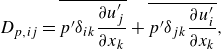 \begin{align}&\qquad\quad D_{p,ij} = \overline {p^{\prime} \delta _{ik} \frac {\partial u^{\prime}_j}{\partial x_k}} + \overline {p^{\prime} \delta _{jk} \frac {\partial u^{\prime}_i}{\partial x_k}}, \end{align}
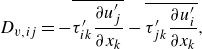 \begin{align}&\qquad\quad D_{v,ij} = - \overline {\tau ^{\prime}_{ik} \frac {\partial u^{\prime}_j}{\partial x_k}} - \overline {\tau ^{\prime}_{jk} \frac {\partial u^{\prime}_i}{\partial x_k}}, \end{align}
 \begin{align}&\quad\,\, D_{\textit{SGS},\textit{ij}} = - \overline {\tau^{\prime}_{ik, {\textit{SGS}}} \frac {\partial u^{\prime}_j}{\partial x_k}} - \overline {\tau^{\prime}_{jk, {\textit{SGS}}} \frac {\partial u^{\prime}_i}{\partial x_k}}. \end{align}
Here $C_{ij}, P_{ij}, T_{t,ij}, T_{p,ij}, T_{v,ij}, T_{\textit{SGS},\textit{ij}}, D_{p,ij}, D_{v,ij}$
and
$C_{ij}, P_{ij}, T_{t,ij}, T_{p,ij}, T_{v,ij}, T_{\textit{SGS},\textit{ij}}, D_{p,ij}, D_{v,ij}$
and $D_{\textit{SGS},\textit{ij}}$
denote convection, production, turbulent transport, pressure transport, viscous transport, SGS transport, pressure redistribution, viscous dissipation and SGS dissipation terms, respectively. As can be seen from (6.3), (6.5)–(6.8), the convection and transport terms are written in conservative forms; that is, they satisfy
$D_{\textit{SGS},\textit{ij}}$
denote convection, production, turbulent transport, pressure transport, viscous transport, SGS transport, pressure redistribution, viscous dissipation and SGS dissipation terms, respectively. As can be seen from (6.3), (6.5)–(6.8), the convection and transport terms are written in conservative forms; that is, they satisfy
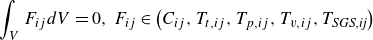 \begin{equation} \int _V F_{ij} dV = 0, \: F_{ij} \in \left ( C_{ij}, T_{t,ij}, T_{p,ij}, T_{v,ij}, T_{\textit{SGS},\textit{ij}} \right ) \end{equation}
for the entire computational domain $V$
. Thus, they do not result in the net increase/decrease in the Reynolds stresses in the flow field. The other terms do not satisfy the above relation, therefore, they act as the source/sink terms of the Reynolds stresses and increase/decrease the Reynolds stresses of the computational domain. The SGS-related terms
$V$
. Thus, they do not result in the net increase/decrease in the Reynolds stresses in the flow field. The other terms do not satisfy the above relation, therefore, they act as the source/sink terms of the Reynolds stresses and increase/decrease the Reynolds stresses of the computational domain. The SGS-related terms $T_{\textit{SGS}, \textit{ij}}$
and
$T_{\textit{SGS}, \textit{ij}}$
and $D_{\textit{SGS}, \textit{ij}}$
represent the direct effects of the employed SGS model on the Reynolds stresses. The other terms are also affected by the change in the SGS-related terms to satisfy the relation
$D_{\textit{SGS}, \textit{ij}}$
represent the direct effects of the employed SGS model on the Reynolds stresses. The other terms are also affected by the change in the SGS-related terms to satisfy the relation $({\partial }/{\partial t}) ( \overline {\rho u^{\prime}_i u^{\prime}_j} ) = 0$
. That is, as the SGS terms increase, the other terms should decrease and vice versa.
$({\partial }/{\partial t}) ( \overline {\rho u^{\prime}_i u^{\prime}_j} ) = 0$
. That is, as the SGS terms increase, the other terms should decrease and vice versa.
Figure 25 shows the budgets of the resolved Reynolds normal stresses for the vLES with the proposed unsupervised–supervised-pipeline SGS model, with the typical SGS model, and the reference DNS by taking $j=i$
. It can be observed that the overall shape of the profiles are similar between the three cases with differences in the magnitude. Focusing on the SGS dissipation term
$j=i$
. It can be observed that the overall shape of the profiles are similar between the three cases with differences in the magnitude. Focusing on the SGS dissipation term $D_{\textit{SGS}, \textit{ii}}$
(dashed blue lines in figure 25), discrepancies are observed between the two SGS models, most evidently for the spanwise component. Furthermore, comparatively large differences in the spanwise viscous dissipation
$D_{\textit{SGS}, \textit{ii}}$
(dashed blue lines in figure 25), discrepancies are observed between the two SGS models, most evidently for the spanwise component. Furthermore, comparatively large differences in the spanwise viscous dissipation $D_{v, 33}$
(solid blue line in figure) and the wall-normal and spanwise pressure redistribution terms
$D_{v, 33}$
(solid blue line in figure) and the wall-normal and spanwise pressure redistribution terms $D_{p, 22}, D_{p,33}$
(solid yellow lines in figure) are observed. Here, based on the discussion in § 6.1, we will focus on the effects of the predicted SGS stresses and the resulting changes to the near-wall wall-normal Reynolds stress, which was found to have significant effects on the correctly predicted near-wall Reynolds shear stress and the mean streamwise velocity in the vLES. Therefore, in the following analyses, the mechanism behind the SGS dissipation and the pressure redistribution are discussed in detail to clarify their roles in predictions of the near-wall wall-normal Reynolds stress.
$D_{p, 22}, D_{p,33}$
(solid yellow lines in figure) are observed. Here, based on the discussion in § 6.1, we will focus on the effects of the predicted SGS stresses and the resulting changes to the near-wall wall-normal Reynolds stress, which was found to have significant effects on the correctly predicted near-wall Reynolds shear stress and the mean streamwise velocity in the vLES. Therefore, in the following analyses, the mechanism behind the SGS dissipation and the pressure redistribution are discussed in detail to clarify their roles in predictions of the near-wall wall-normal Reynolds stress.
Figure 25. Budgets of Reynolds normal stresses in a posteriori tests at $Re_\tau \approx 1000$
. (a–c) Streamwise component; (d–f) wall-normal component; (g–i) spanwise component; (a,d,g) vLES with proposed unsupervised–supervised-pipeline SGS model; (b,e,h) vLES with typical SGS model; (c,f,i) reference DNS. Solid red, production
$Re_\tau \approx 1000$
. (a–c) Streamwise component; (d–f) wall-normal component; (g–i) spanwise component; (a,d,g) vLES with proposed unsupervised–supervised-pipeline SGS model; (b,e,h) vLES with typical SGS model; (c,f,i) reference DNS. Solid red, production $P_{ij}$
; solid green, turbulent diffusion
$P_{ij}$
; solid green, turbulent diffusion $T_{t,ij}$
; solid orange, pressure diffusion
$T_{t,ij}$
; solid orange, pressure diffusion $T_{p,ij}$
; solid purple, viscous diffusion
$T_{p,ij}$
; solid purple, viscous diffusion $T_{v,ij}$
; dashed purple, SGS diffusion
$T_{v,ij}$
; dashed purple, SGS diffusion $T_{\textit{SGS},\textit{ij}}$
; solid yellow, pressure redistribution
$T_{\textit{SGS},\textit{ij}}$
; solid yellow, pressure redistribution $D_{p,ij}$
; solid blue, viscous dissipation
$D_{p,ij}$
; solid blue, viscous dissipation $D_{v,ij}$
; dashed blue, SGS dissipation
$D_{v,ij}$
; dashed blue, SGS dissipation $D_{\textit{SGS},\textit{ij}}$
.
$D_{\textit{SGS},\textit{ij}}$
.
First, the effects of the SGS dissipation term ( $D_{\textit{SGS}, \textit{ii}}$
, dashed blue lines in figure) are discussed. In the wall-normal component of the SGS dissipation term
$D_{\textit{SGS}, \textit{ii}}$
, dashed blue lines in figure) are discussed. In the wall-normal component of the SGS dissipation term $D_{\textit{SGS}, 22}$
, there is little difference between the SGS models (and also
$D_{\textit{SGS}, 22}$
, there is little difference between the SGS models (and also $D_{\textit{SGS}, 22}$
is negligibly small), suggesting that the near-wall differences in the wall-normal Reynolds stress are not directly caused by the SGS dissipation term
$D_{\textit{SGS}, 22}$
is negligibly small), suggesting that the near-wall differences in the wall-normal Reynolds stress are not directly caused by the SGS dissipation term $D_{\textit{SGS}, 22}$
. On the other hand, the spanwise SGS dissipation term
$D_{\textit{SGS}, 22}$
. On the other hand, the spanwise SGS dissipation term $D_{\textit{SGS},33}$
shows opposite tendencies between the proposed unsupervised–supervised-pipeline SGS model and the conventional SGS model. The conventional SGS model predicts negative values of the SGS dissipation, whereas the proposed unsupervised–supervised-pipeline SGS model predicts positive values in the near-wall region (
$D_{\textit{SGS},33}$
shows opposite tendencies between the proposed unsupervised–supervised-pipeline SGS model and the conventional SGS model. The conventional SGS model predicts negative values of the SGS dissipation, whereas the proposed unsupervised–supervised-pipeline SGS model predicts positive values in the near-wall region ( $y^+ \lesssim 100$
). In general, positive values in the SGS dissipation term (i.e. the net increase in the resolved Reynolds stress) are attributed to the occurrences of SGS backscatter events; that is, the resolved Reynolds stress is transported from the unresolved SGS components. The results suggest that the increased near-wall spanwise Reynolds stress predicted by the proposed unsupervised–supervised-pipeline SGS model seen in figure 23 is primarily caused by the SGS backscatter, which induces the near-wall spanwise velocity fluctuations.
$y^+ \lesssim 100$
). In general, positive values in the SGS dissipation term (i.e. the net increase in the resolved Reynolds stress) are attributed to the occurrences of SGS backscatter events; that is, the resolved Reynolds stress is transported from the unresolved SGS components. The results suggest that the increased near-wall spanwise Reynolds stress predicted by the proposed unsupervised–supervised-pipeline SGS model seen in figure 23 is primarily caused by the SGS backscatter, which induces the near-wall spanwise velocity fluctuations.
Next, we focus on the pressure redistribution term $D_{p,ii}$
(yellow lines in figure). In the incompressible limit, this term satisfies
$D_{p,ii}$
(yellow lines in figure). In the incompressible limit, this term satisfies $\sum _{i} D_{p,ii} = 0$
. Therefore, this term represents the exchange of Reynolds normal stress components between each other. Note that the vertical axis ranges vary among the three components depicted in figure 25. Particularly, the wall-normal component (figure 25
d–f) exhibits the smallest range among the three directions. In the near-wall region (
$\sum _{i} D_{p,ii} = 0$
. Therefore, this term represents the exchange of Reynolds normal stress components between each other. Note that the vertical axis ranges vary among the three components depicted in figure 25. Particularly, the wall-normal component (figure 25
d–f) exhibits the smallest range among the three directions. In the near-wall region ( $20 \lesssim y^+ \lesssim 100$
) of the proposed unsupervised–supervised-pipeline SGS model, the spanwise component shows a negative value while the wall-normal component shows a positive value. The decrease of the spanwise stress and the increase of the wall-normal stress corresponds to the transfer of the Reynolds stress from the spanwise component to the wall-normal component through the pressure redistribution term. In fact, this process is known to be the dominant energy transfer mechanism towards the wall-normal component (Lee & Moser Reference Lee and Moser2019), and will be discussed in more detail in § 6.2.2. In comparison, the conventional SGS model predicts a smaller positive peak in the wall-normal component slightly farther from the wall (
$20 \lesssim y^+ \lesssim 100$
) of the proposed unsupervised–supervised-pipeline SGS model, the spanwise component shows a negative value while the wall-normal component shows a positive value. The decrease of the spanwise stress and the increase of the wall-normal stress corresponds to the transfer of the Reynolds stress from the spanwise component to the wall-normal component through the pressure redistribution term. In fact, this process is known to be the dominant energy transfer mechanism towards the wall-normal component (Lee & Moser Reference Lee and Moser2019), and will be discussed in more detail in § 6.2.2. In comparison, the conventional SGS model predicts a smaller positive peak in the wall-normal component slightly farther from the wall ( $y^+ \approx 70$
) compared with the proposed unsupervised–supervised-pipeline SGS model. This shows that the redistribution of the Reynolds stress to the wall-normal component is weaker and occurs farther away from the wall using the conventional SGS model. It can be considered that these differences between the SGS models in the pressure redistribution term are the causes of the differences in the near-wall wall-normal and the shear Reynolds stresses.
$y^+ \approx 70$
) compared with the proposed unsupervised–supervised-pipeline SGS model. This shows that the redistribution of the Reynolds stress to the wall-normal component is weaker and occurs farther away from the wall using the conventional SGS model. It can be considered that these differences between the SGS models in the pressure redistribution term are the causes of the differences in the near-wall wall-normal and the shear Reynolds stresses.
Considering that the terms in (6.2) balance each other out to satisfy ${(\partial }/{\partial t}) ( \overline {\rho u^{\prime}_i u^{\prime}_i} ) = 0$
, the prediction of SGS backscatter by the proposed SGS model in the near-wall spanwise Reynolds stress leads to a net decrease in the other terms. In the present vLES, the decrease was observed for the pressure redistribution term, which represents the outflow of Reynolds stress from the spanwise component. The decrease then leads to the increase of the pressure redistribution term in the near-wall wall-normal component to satisfy
${(\partial }/{\partial t}) ( \overline {\rho u^{\prime}_i u^{\prime}_i} ) = 0$
, the prediction of SGS backscatter by the proposed SGS model in the near-wall spanwise Reynolds stress leads to a net decrease in the other terms. In the present vLES, the decrease was observed for the pressure redistribution term, which represents the outflow of Reynolds stress from the spanwise component. The decrease then leads to the increase of the pressure redistribution term in the near-wall wall-normal component to satisfy $\sum _{i} D_{p,ii} = 0$
, acting as the source term for the increasing wall-normal velocity fluctuations. Therefore, it can be considered that the increase in the near-wall wall-normal Reynolds stress is caused by the SGS backscatter in the near-wall spanwise Reynolds stress. The increase of the near-wall spanwise Reynolds stress leads to the increase of the near-wall Reynolds shear stress and the resultant correct mean velocity. On the other hand, the typical SGS model does not predict the SGS backscatter in the spanwise Reynolds stress and resultantly does not cause the redistribution of near-wall Reynolds stresses from the spanwise to the wall-normal component. Therefore, the conventional SGS model leads to a smaller wall-normal Reynolds stress in the near-wall region, leading to the underprediction of the near-wall Reynolds shear stress and the overprediction of the mean streamwise velocity.
$\sum _{i} D_{p,ii} = 0$
, acting as the source term for the increasing wall-normal velocity fluctuations. Therefore, it can be considered that the increase in the near-wall wall-normal Reynolds stress is caused by the SGS backscatter in the near-wall spanwise Reynolds stress. The increase of the near-wall spanwise Reynolds stress leads to the increase of the near-wall Reynolds shear stress and the resultant correct mean velocity. On the other hand, the typical SGS model does not predict the SGS backscatter in the spanwise Reynolds stress and resultantly does not cause the redistribution of near-wall Reynolds stresses from the spanwise to the wall-normal component. Therefore, the conventional SGS model leads to a smaller wall-normal Reynolds stress in the near-wall region, leading to the underprediction of the near-wall Reynolds shear stress and the overprediction of the mean streamwise velocity.
6.2.2. Mechanisms of redistribution of Reynolds stresses
In § 6.2.1, the SGS dissipation and the pressure redistribution terms are shown to have a significant effect on the prediction of the mean velocity and the Reynolds shear stress by the proposed unsupervised–supervised-pipeline SGS model. The redistribution of the stress from the spanwise to the wall-normal component is to be expected from streamwise vortices near the wall (Lee & Moser Reference Lee and Moser2019), as shown in figure 26. For example, at locations with $({\partial v^{\prime}}/{\partial y})\gt 0$
(red regions in figure), the spanwise velocity satisfies
$({\partial v^{\prime}}/{\partial y})\gt 0$
(red regions in figure), the spanwise velocity satisfies $({\partial w^{\prime}}/{\partial z})\lt 0$
. Conversely, at blue regions in the figure,
$({\partial w^{\prime}}/{\partial z})\lt 0$
. Conversely, at blue regions in the figure, $({\partial v^{\prime}}/{\partial y})\gt 0$
and
$({\partial v^{\prime}}/{\partial y})\gt 0$
and $({\partial w^{\prime}}/{\partial z})\lt 0$
are satisfied. Therefore,
$({\partial w^{\prime}}/{\partial z})\lt 0$
are satisfied. Therefore, $p^{\prime} ({\partial v^{\prime}}/{\partial y})$
and
$p^{\prime} ({\partial v^{\prime}}/{\partial y})$
and $p^{\prime} ({\partial w^{\prime}}/{\partial z)}$
have opposite signs at each of the red and blue regions which represent the redistribution of the Reynolds normal stress as discussed earlier. However, because the grid resolutions between the DNS and vLES are different by a factor of eight, the resolved structures of the near-wall turbulence are also expected to be different. Here, we perform the spectral analyses of the pressure redistribution terms to quantify the differences between the resolved turbulence in vLES using the proposed unsupervised–supervised-pipeline SGS model and the conventional SGS. Specifically, we aim to elucidate the reason of the differences in the pressure redistribution terms by examining the spanwise wavelengths (denoted by
$p^{\prime} ({\partial w^{\prime}}/{\partial z)}$
have opposite signs at each of the red and blue regions which represent the redistribution of the Reynolds normal stress as discussed earlier. However, because the grid resolutions between the DNS and vLES are different by a factor of eight, the resolved structures of the near-wall turbulence are also expected to be different. Here, we perform the spectral analyses of the pressure redistribution terms to quantify the differences between the resolved turbulence in vLES using the proposed unsupervised–supervised-pipeline SGS model and the conventional SGS. Specifically, we aim to elucidate the reason of the differences in the pressure redistribution terms by examining the spanwise wavelengths (denoted by $\lambda _z$
in figure) associated with these structures.
$\lambda _z$
in figure) associated with these structures.
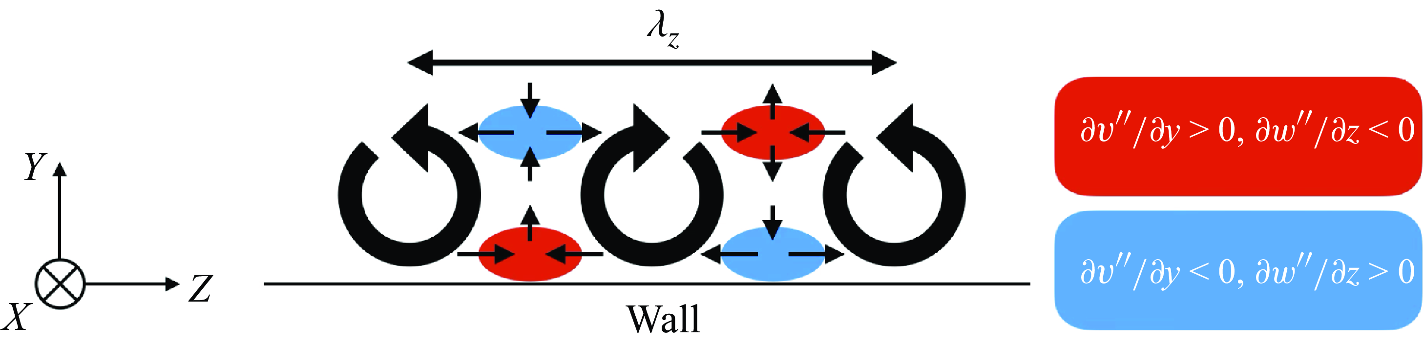
Figure 26. Schematic of near-wall streaky streamwise vortices in wall turbulence.
As with § 6.2.1, we disregard the density variations because of the low Mach number condition at $M_b \approx 0.1$
. Considering the channel flow as in this study in which the flow is homogeneous in the streamwise and the spanwise directions, the spectral Reynolds stress budget equation (Mizuno Reference Mizuno2016; Lee & Moser Reference Lee and Moser2019) can be written as
$M_b \approx 0.1$
. Considering the channel flow as in this study in which the flow is homogeneous in the streamwise and the spanwise directions, the spectral Reynolds stress budget equation (Mizuno Reference Mizuno2016; Lee & Moser Reference Lee and Moser2019) can be written as
 \begin{align} \textrm{Re} \left [ \frac {\partial }{\partial t} \left (\overline {\rho \widehat {u^{\prime}_i} \widehat {u^{\prime}_j}^* } \right ) \right ] = & \check C_{ij} + \check P_{ij} + \check T_{t,ij} + \check T_{p,ij} + \check T_{v,ij} + \check T_{\textit{SGS},\textit{ij}} \nonumber \\ & + \check D_{p,ij} + \check D_{v,ij} + \check D_{\textit{SGS},\textit{ij}}. \end{align}
Here, $\widehat {(\cdot )}$
denotes the Fourier transformed quantity,
$\widehat {(\cdot )}$
denotes the Fourier transformed quantity, $(\cdot )^*$
the complex conjugate and
$(\cdot )^*$
the complex conjugate and $\textrm{Re} [\cdot ]$
the real part of the complex number. For each term on the right-hand side, the following equality holds:
$\textrm{Re} [\cdot ]$
the real part of the complex number. For each term on the right-hand side, the following equality holds:
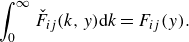 \begin{equation} \int _{0}^{\infty } \check F_{ij} (k,y) {\textrm d}k = F_{ij}(y). \end{equation}
This equation shows that the terms in the spectral budget equation represents the contribution of each wavenumber to the budget term in the total budget equation (6.2). Note that the previous studies (Mizuno Reference Mizuno2016; Lee & Moser Reference Lee and Moser2019) further split the turbulent transport term $\check T_{t,ij}$
into the spatial and interscale transfers, which is not employed here for consistency with (6.2). Following the discussion in § 6.2.1, we focus on the spectral pressure redistribution term
$\check T_{t,ij}$
into the spatial and interscale transfers, which is not employed here for consistency with (6.2). Following the discussion in § 6.2.1, we focus on the spectral pressure redistribution term $\check D_{p,ij}$
which is written as
$\check D_{p,ij}$
which is written as
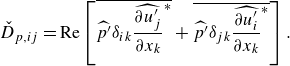 \begin{equation} \check D_{p,ij} = \textrm{Re} \left [ \overline {\widehat {p^{\prime}} \delta _{ik} \widehat {\frac {\partial u^{\prime}_j}{\partial x_k}}^*} + \overline {\widehat {p^{\prime}} \delta _{jk} \widehat {\frac {\partial u^{\prime}_i}{\partial x_k}}^*} \right ]. \end{equation}
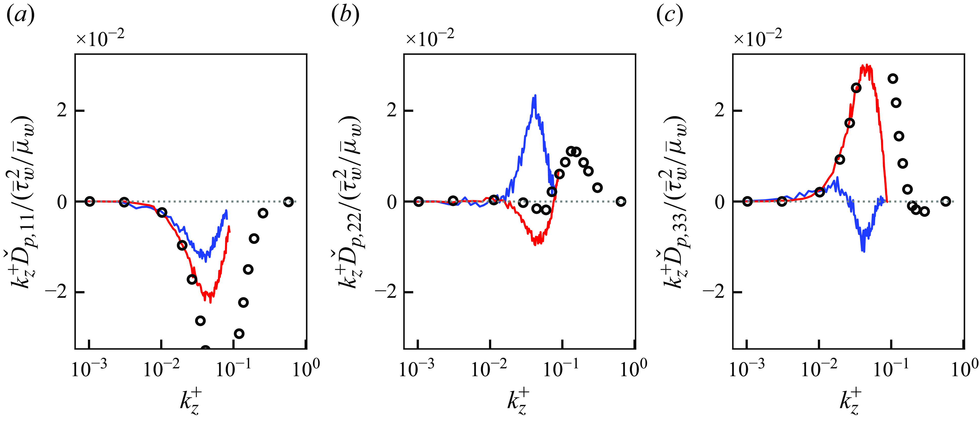
Figure 27. Premultiplied spanwise-spectral components of pressure redistribution in a posteriori tests at $y^+ \approx 15$
at
$y^+ \approx 15$
at $Re_\tau \approx 1000$
. (a) Streamwise component; (b) wall-normal component; (c) spanwise component. Blue lines, proposed unsupervised–supervised-pipeline SGS model; red lines, typical SGS model, circles, reference DNS. Horizontal dotted lines denote values of
$Re_\tau \approx 1000$
. (a) Streamwise component; (b) wall-normal component; (c) spanwise component. Blue lines, proposed unsupervised–supervised-pipeline SGS model; red lines, typical SGS model, circles, reference DNS. Horizontal dotted lines denote values of $0$
in the vertical axes.
$0$
in the vertical axes.
Figure 27 shows the premultiplied spanwise spectral components of the pressure redistribution term for the proposed unsupervised–supervised-pipeline SGS model, the conventional SGS model and the reference DNS at the $y^+ \approx 15$
plane. In the DNS, the wall-normal component of the pressure redistribution term takes a positive peak in the high-wavenumber range of
$y^+ \approx 15$
plane. In the DNS, the wall-normal component of the pressure redistribution term takes a positive peak in the high-wavenumber range of $k_z^+ \gtrsim 0.1$
. There also exists a small negative peak in the spanwise component in this high-wavenumber range. As also discussed by Lee & Moser (Reference Lee and Moser2019), these peaks show that there is the redistribution of the Reynolds stress from the spanwise direction to the wall-normal direction, and the near-wall streaky streamwise vortices discussed above occur in the spanwise wavelength of
$k_z^+ \gtrsim 0.1$
. There also exists a small negative peak in the spanwise component in this high-wavenumber range. As also discussed by Lee & Moser (Reference Lee and Moser2019), these peaks show that there is the redistribution of the Reynolds stress from the spanwise direction to the wall-normal direction, and the near-wall streaky streamwise vortices discussed above occur in the spanwise wavelength of $\lambda _z^+ \lesssim 2 \pi / k_z^+ \approx 60$
. Here, it is notable that the spanwise grid spacings for the vLES are set at
$\lambda _z^+ \lesssim 2 \pi / k_z^+ \approx 60$
. Here, it is notable that the spanwise grid spacings for the vLES are set at $\Delta z ^+ \approx 36$
and therefore cannot resolve the structures smaller than the Nyquist wavelength
$\Delta z ^+ \approx 36$
and therefore cannot resolve the structures smaller than the Nyquist wavelength $2 \Delta z^+ \approx 72$
. This is shown in the figure by the fact that the solid lines do not exist in the high-wavenumber range
$2 \Delta z^+ \approx 72$
. This is shown in the figure by the fact that the solid lines do not exist in the high-wavenumber range $k^+ \gtrsim 0.09$
. Instead, the proposed unsupervised–supervised-pipeline SGS model shows a clear positive peak of the spanwise pressure redistribution term at the smaller wavenumber of
$k^+ \gtrsim 0.09$
. Instead, the proposed unsupervised–supervised-pipeline SGS model shows a clear positive peak of the spanwise pressure redistribution term at the smaller wavenumber of $k_z^+ \approx 0.04$
, for which the corresponding wavelength at
$k_z^+ \approx 0.04$
, for which the corresponding wavelength at $\lambda _z^+ = 2 \pi / k_z^+ \approx 160$
is larger than the DNS. There is also a negative peak in the spanwise pressure redistribution term at the similar wavenumber range, suggesting that there exist dominant near-wall streaky streamwise vortical structures at this wavenumber range. These observations can be understood as the mechanism by which the near-wall wall-normal Reynolds stress increases for the proposed unsupervised–supervised-pipeline SGS model; that is, the pressure redistribution of near-wall Reynolds normal stress from the spanwise to wall-normal component is driven by the larger vortical structures. As discussed in § 6.2.1, the redistribution leads to the increase of the near-wall wall-normal Reynolds stress and the Reynolds shear stress, resulting in the correct prediction of the mean streamwise velocity. On the other hand, it can be seen from the wall-normal budget of the conventional SGS model that the positive peak of the pressure redistribution term does not exist in the wall-normal component. The lack of redistribution towards the wall-normal component causes the discrepancies in the near-wall wall-normal Reynolds stress and Reynolds shear stress, leading to the overprediction of the mean streamwise velocity.
$\lambda _z^+ = 2 \pi / k_z^+ \approx 160$
is larger than the DNS. There is also a negative peak in the spanwise pressure redistribution term at the similar wavenumber range, suggesting that there exist dominant near-wall streaky streamwise vortical structures at this wavenumber range. These observations can be understood as the mechanism by which the near-wall wall-normal Reynolds stress increases for the proposed unsupervised–supervised-pipeline SGS model; that is, the pressure redistribution of near-wall Reynolds normal stress from the spanwise to wall-normal component is driven by the larger vortical structures. As discussed in § 6.2.1, the redistribution leads to the increase of the near-wall wall-normal Reynolds stress and the Reynolds shear stress, resulting in the correct prediction of the mean streamwise velocity. On the other hand, it can be seen from the wall-normal budget of the conventional SGS model that the positive peak of the pressure redistribution term does not exist in the wall-normal component. The lack of redistribution towards the wall-normal component causes the discrepancies in the near-wall wall-normal Reynolds stress and Reynolds shear stress, leading to the overprediction of the mean streamwise velocity.
6.2.3. Discussions on the near-wall turbulence mechanisms
Based on the above analyses of the Reynolds stress budget, we discuss the differences in the resolved phenomena that leads to the differences in the near-wall Reynolds shear stress between the high-fidelity DNS and vLES with the proposed unsupervised–supervised-pipeline SGS model and the conventional SGS model.
We first discuss the DNS, which is a high-fidelity representation of real turbulence. As also shown by Lee & Moser (Reference Lee and Moser2019), near-wall wall-normal Reynolds stress is generated primarily by the pressure redistribution from the spanwise Reynolds stress. The redistribution occurs in the spanwise wavenumber of $k_z^+ \approx 60$
. The resulting increase in the wall-normal stress gives rise to the Reynolds shear stress in the near-wall buffer layer of the turbulent boundary layer.
$k_z^+ \approx 60$
. The resulting increase in the wall-normal stress gives rise to the Reynolds shear stress in the near-wall buffer layer of the turbulent boundary layer.
In the vLES using the proposed unsupervised–supervised-pipeline SGS model, the SGS backscatter represented by the positive SGS dissipation term (SGS backscatter) introduces the additional production of the resolved Reynolds stress in the spanwise direction, as shown in figure 25. The effect of the predicted SGS backscatter can also be seen in the instantaneous flow fields in figure 24, where the non-physical large elongated structures in the near-wall region such as those observed by the conventional SGS model are disturbed to generate the smaller structures. To satisfy the balance of the Reynolds stress budget (6.2), the increased near-wall spanwise stress then gives rise to the increased pressure redistribution towards the wall-normal stress which results in the increased near-wall wall-normal Reynolds stress and Reynolds shear stress. Here, the spectral budgets (figure 27) show that the redistribution mainly occurs in the spanwise wavenumbers of $0.03 \lesssim k_z^+ \lesssim 0.05$
, which correspond to the resolved wavelengths of
$0.03 \lesssim k_z^+ \lesssim 0.05$
, which correspond to the resolved wavelengths of $3.5 \Delta z \lesssim \lambda _z \lesssim 5.8 \Delta z$
(
$3.5 \Delta z \lesssim \lambda _z \lesssim 5.8 \Delta z$
( $130 \lesssim \lambda _z^+ \lesssim 210$
). While these length scales are larger than those observed in the DNS because of the very coarse grid employed in the vLES, the resolved turbulent structures serve the similar roles in the redistribution of the Reynolds normal stresses. Here we repeat that the spanwise wavenumber for DNS (
$130 \lesssim \lambda _z^+ \lesssim 210$
). While these length scales are larger than those observed in the DNS because of the very coarse grid employed in the vLES, the resolved turbulent structures serve the similar roles in the redistribution of the Reynolds normal stresses. Here we repeat that the spanwise wavenumber for DNS ( $k_z^+ \approx 60$
) cannot be resolved by the vLES grid. Considering that the redistribution process is induced by the predicted SGS backscatter, the increased wall-normal stress can thus be interpreted as compensation for the unresolved turbulence dynamics by the proposed SGS model. As a result, although the resolved flow field of vLES cannot reproduce the near-wall turbulent physics of DNS (because of the very coarse grid), the vLES with the proposed unsupervised–supervised-pipeline SGS model leads to the accurate near-wall Reynolds shear stress and the resultant mean streamwise velocity profile.
$k_z^+ \approx 60$
) cannot be resolved by the vLES grid. Considering that the redistribution process is induced by the predicted SGS backscatter, the increased wall-normal stress can thus be interpreted as compensation for the unresolved turbulence dynamics by the proposed SGS model. As a result, although the resolved flow field of vLES cannot reproduce the near-wall turbulent physics of DNS (because of the very coarse grid), the vLES with the proposed unsupervised–supervised-pipeline SGS model leads to the accurate near-wall Reynolds shear stress and the resultant mean streamwise velocity profile.
In the vLES using the conventional SGS model, where the turbulence physics in the unresolved wavenumbers $k_z^+ \gtrsim 0.09$
that are crucial for the reproduction of the near-wall wall-normal Reynolds stress are also not resolved, the redistribution of Reynolds stress from the spanwise to the wall-normal component does not occur in the near-wall region. As the conventional SGS model fails to reproduce the near-wall energy redistribution that is crucial for the accurate prediction of the Reynolds shear stress, the mean streamwise velocity resultantly shifts to satisfy the total shear stress balance, leading to the overprediction of velocity.
$k_z^+ \gtrsim 0.09$
that are crucial for the reproduction of the near-wall wall-normal Reynolds stress are also not resolved, the redistribution of Reynolds stress from the spanwise to the wall-normal component does not occur in the near-wall region. As the conventional SGS model fails to reproduce the near-wall energy redistribution that is crucial for the accurate prediction of the Reynolds shear stress, the mean streamwise velocity resultantly shifts to satisfy the total shear stress balance, leading to the overprediction of velocity.
We also note that the identified mechanisms of the proposed unsupervised–supervised-pipeline SGS model show similarities with the SGS dynamics described by Hamba (Reference Hamba2019) and Inagaki & Kobayashi (Reference Inagaki and Kobayashi2023). By analysing the DNS data of turbulent channel flows, it was shown that SGS backscatter in the spanwise velocity fluctuations occur in the near-wall region. It is also shown that the physics-based stabilised mixed SGS model proposed by Abe (Reference Abe2013) enables appropriate prediction of the redistribution term for the near-wall wall-normal Reynolds stress in coarse-grid LES, which leads to the enhanced near-wall Reynolds shear stress (Inagaki & Kobayashi Reference Inagaki and Kobayashi2020). As these observations are consistent with the identified near-wall dynamics of the proposed unsupervised–supervised-pipeline SGS model in this study, we believe that the spanwise SGS backscatter and the pressure redistribution terms may provide insight into further development of SGS models for coarse-grid LES.
7. Robustness against Reynolds number higher than training data
As discussed in § 4.1, the machine learning models (i.e. unsupervised model $G_{\textit{vLES}-\textit{fDNS}}$
and supervised model
$G_{\textit{vLES}-\textit{fDNS}}$
and supervised model $G_{\textit{SR}}$
in figure 3) in the proposed unsupervised–supervised-pipeline SGS model are trained using flow fields at the friction Reynolds number of
$G_{\textit{SR}}$
in figure 3) in the proposed unsupervised–supervised-pipeline SGS model are trained using flow fields at the friction Reynolds number of $Re_\tau \approx 1000$
. Here, we apply the same models to an LES simulation at a higher Reynolds number than the training data; namely,
$Re_\tau \approx 1000$
. Here, we apply the same models to an LES simulation at a higher Reynolds number than the training data; namely, $Re_\tau \approx 2000$
to assess the extrapolation capabilities of the proposed machine-learning SGS model to different flow conditions that it was not trained on. The computational grid for the
$Re_\tau \approx 2000$
to assess the extrapolation capabilities of the proposed machine-learning SGS model to different flow conditions that it was not trained on. The computational grid for the $Re_\tau \approx 2000$
case is constructed in the same manner as described in § 4.1 and summarised in table 2.
$Re_\tau \approx 2000$
case is constructed in the same manner as described in § 4.1 and summarised in table 2.
Table 2. List of parameters for each computational set-up. Here $L_x$
,
$L_x$
, $L_z$
and
$L_z$
and $L_y$
denote computational domain size. Here
$L_y$
denote computational domain size. Here $\Delta x$
,
$\Delta x$
, $\Delta y$
and
$\Delta y$
and $\Delta z$
denote grid resolutions in each direction, and superscript
$\Delta z$
denote grid resolutions in each direction, and superscript $(\cdot )^+$
represents values in wall units. Here
$(\cdot )^+$
represents values in wall units. Here $N_x$
,
$N_x$
, $N_z$
and
$N_z$
and $N_y$
denote number of grid points in each direction.
$N_y$
denote number of grid points in each direction.
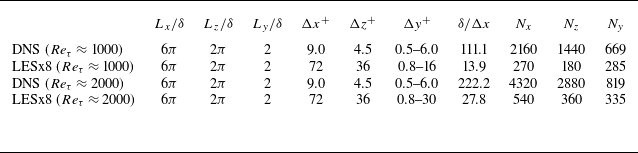
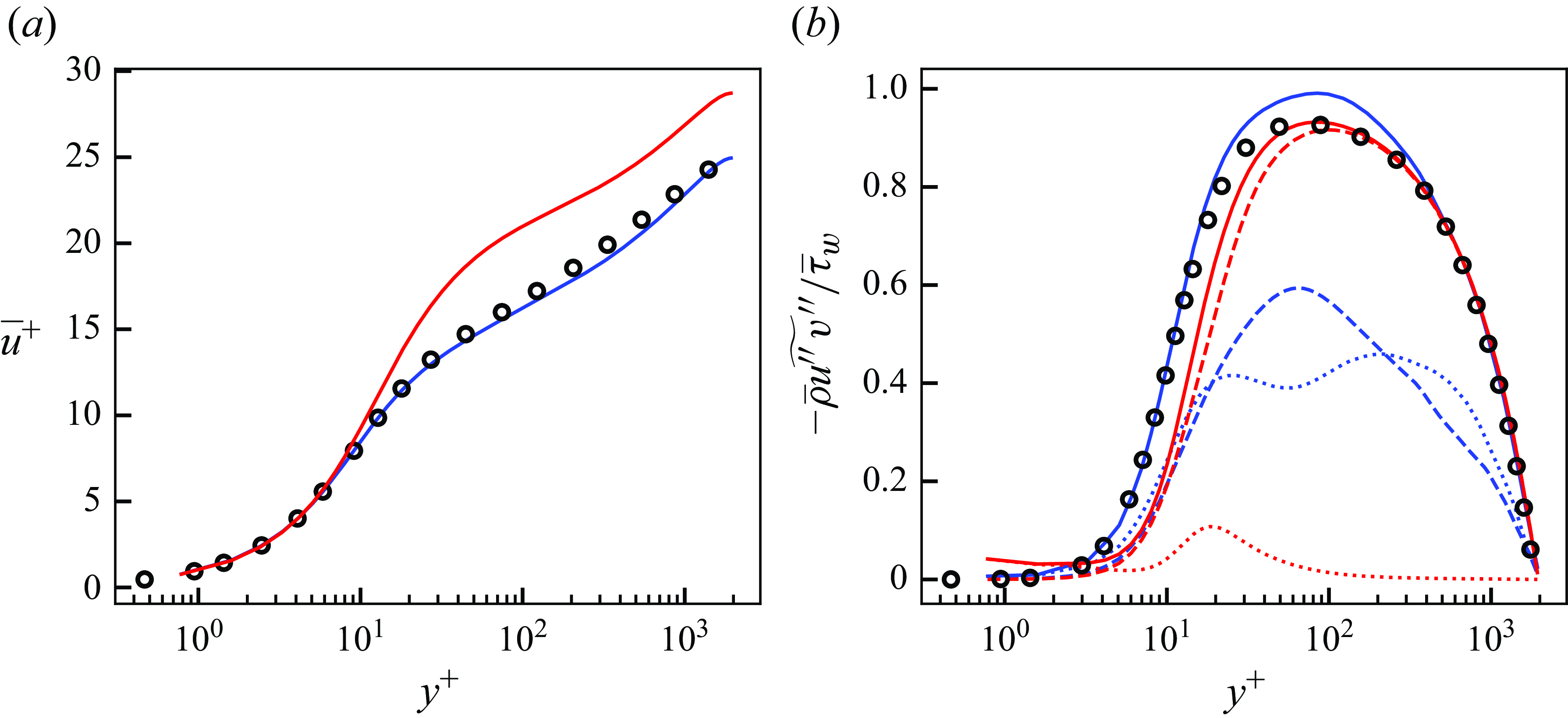
Figure 28. Mean streamwise velocity (a) and Reynolds shear stress (b) of a posteriori tests at $Re_\tau \approx 2000$
. Blue, vLES with proposed unsupervised–supervised-pipeline SGS model; red, vLES with typical SGS model; black circles, reference DNS. For (b): dashed lines, resolved component; dotted lines, SGS component; solid lines, total stress.
$Re_\tau \approx 2000$
. Blue, vLES with proposed unsupervised–supervised-pipeline SGS model; red, vLES with typical SGS model; black circles, reference DNS. For (b): dashed lines, resolved component; dotted lines, SGS component; solid lines, total stress.

Figure 29. Streamwise (a), wall-normal (b) and spanwise (c) Reynolds stresses of a posteriori tests at $Re_\tau \approx 2000$
. Blue, vLES with proposed unsupervised–supervised-pipeline SGS model; red, vLES with typical SGS model; black circles, reference DNS. Dashed lines, resolved component; dotted lines, SGS component; solid lines, resolved + SGS stress.
$Re_\tau \approx 2000$
. Blue, vLES with proposed unsupervised–supervised-pipeline SGS model; red, vLES with typical SGS model; black circles, reference DNS. Dashed lines, resolved component; dotted lines, SGS component; solid lines, resolved + SGS stress.
The obtained mean streamwise velocity and the Reynolds shear stress are shown in figure 28. The proposed unsupervised–supervised-pipeline SGS model shows good agreement with the reference DNS in the predicted velocity and the near-wall shear stress even for the flow condition that the machine learning models were not trained on, which shows the robustness of the proposed machine-learning-based model. On the other hand, the conventional SGS model shows significant deviations in the mean streamwise velocity and the near-wall Reynolds shear stress. The obtained Reynolds normal stresses are summarised in figure 29. The predicted stresses obtained by both the SGS models show similar tendencies to the $Re_\tau \approx 1000$
case, such as the similar profiles of the streamwise stress
$Re_\tau \approx 1000$
case, such as the similar profiles of the streamwise stress $\overline {\rho } \widetilde {u^{\prime\prime}u^{\prime\prime}}$
and the larger wall-normal stress
$\overline {\rho } \widetilde {u^{\prime\prime}u^{\prime\prime}}$
and the larger wall-normal stress $\overline {\rho } \widetilde {v^{\prime\prime}v^{\prime\prime}}$
predicted by the proposed unsupervised–supervised-pipeline SGS model in the near-wall region. Likewise, the Reynolds shear stress correctly rises in the near-wall region for the proposed model leading to the better prediction of the mean streamwise velocity, while the conventional SGS model underpredicts the near-wall Reynolds shear stress causing overprediction of the mean velocity. These similarities suggest that, despite the Reynolds number differences, the proposed unsupervised–supervised-pipeline SGS model functions in a similar mechanism to the
$\overline {\rho } \widetilde {v^{\prime\prime}v^{\prime\prime}}$
predicted by the proposed unsupervised–supervised-pipeline SGS model in the near-wall region. Likewise, the Reynolds shear stress correctly rises in the near-wall region for the proposed model leading to the better prediction of the mean streamwise velocity, while the conventional SGS model underpredicts the near-wall Reynolds shear stress causing overprediction of the mean velocity. These similarities suggest that, despite the Reynolds number differences, the proposed unsupervised–supervised-pipeline SGS model functions in a similar mechanism to the $Re_\tau \approx 1000$
case to enable the accurate predictions of the Reynolds shear stress and the resultant mean streamwise velocity. Furthermore, it suggests that the DNS data of a low-Reynolds number turbulence, which are relatively low-cost and feasible to obtain, can be used to train a machine learning model to enable vLES of high-Reynolds number turbulence for which DNS is prohibitively expensive.
$Re_\tau \approx 1000$
case to enable the accurate predictions of the Reynolds shear stress and the resultant mean streamwise velocity. Furthermore, it suggests that the DNS data of a low-Reynolds number turbulence, which are relatively low-cost and feasible to obtain, can be used to train a machine learning model to enable vLES of high-Reynolds number turbulence for which DNS is prohibitively expensive.
This test shows that the proposed unsupervised–supervised-pipeline methodology can be successfully applied to Reynolds numbers that are higher than the training data. By employing the CNNs as in this study, the machine-learning models are able to incorporate the spatial extent of the non-physical turbulent structures to accurately predict the SGS stresses. On the other hand, pointwise predictions (for example by using the local velocity gradient tensor as the input features as demonstrated by Gamahara & Hattori (Reference Gamahara and Hattori2017)) may not be able to appropriately distinguish the non-physical structures. It should be noted that for both the training data and testing, the computational grids are constructed in wall-units (normalised by the wall shear stress $\tau _w$
and the viscosity at the wall
$\tau _w$
and the viscosity at the wall $\mu _w$
). Therefore, the near-wall turbulent structures characterised by the wall-unit are resolved by nearly the same number of grid points for both Reynolds number cases. Because this study employs CNNs which operate in the computational coordinate space as the components of the machine learning models (see Appendix A), it is important to keep the resolution of the turbulence structures similar between the training and the testing. This limitation of the CNNs may degrade the applicability of the presented model to different grid resolutions and aspect ratios from the training data, and require additional work for use in unstructured grids. Although this problem may be overcome by machine learning techniques such as transfer learning (as has been pursued by Guan et al. (Reference Guan, Chattopadhyay, Subel and Hassanzadeh2022)), we see this problem as a problem of the CNN architecture itself and not particular to the proposed unsupervised–supervised-pipeline methodology.
$\mu _w$
). Therefore, the near-wall turbulent structures characterised by the wall-unit are resolved by nearly the same number of grid points for both Reynolds number cases. Because this study employs CNNs which operate in the computational coordinate space as the components of the machine learning models (see Appendix A), it is important to keep the resolution of the turbulence structures similar between the training and the testing. This limitation of the CNNs may degrade the applicability of the presented model to different grid resolutions and aspect ratios from the training data, and require additional work for use in unstructured grids. Although this problem may be overcome by machine learning techniques such as transfer learning (as has been pursued by Guan et al. (Reference Guan, Chattopadhyay, Subel and Hassanzadeh2022)), we see this problem as a problem of the CNN architecture itself and not particular to the proposed unsupervised–supervised-pipeline methodology.
8. Conclusion
We proposed an unsupervised-and-supervised machine learning pipeline which enables SGS modelling for vLES, where the energetic eddies that are resolved in regular LES are not properly resolved by the grid. As a consequence, the coarse grid resolves turbulent structures that are not similar to the structures from fDNS data. Our proposed pipeline consists of an unsupervised vLES-to-fDNS model using CycleGAN, which transforms the input non-physical vLES flow fields to physical fDNS quality, and a supervised super-resolution model using cGAN, which super-resolves the fDNS-quality flow fields to obtain the DNS-quality flow fields. To accurately super-resolve the vLES flow fields which show dissimilar turbulent statistics from the fDNS, the proposed pipeline is trained unsupervisedly using vLES flow fields in its dataset. The use of unsupervised learning is mandated by the fact that it is impossible to obtain the paired data of the instantaneous vLES flow fields and their expected DNS outputs, which inhibits the use of typical supervised machine-learning super-resolution methods.
The proposed unsupervised–supervised pipeline was trained and tested in both a priori and a posteriori tests using the simulations of a turbulent channel flow at $Re_\tau \approx 1000, M_b \approx 0.1$
. The a posteriori test was also performed at the higher Reynolds number of
$Re_\tau \approx 1000, M_b \approx 0.1$
. The a posteriori test was also performed at the higher Reynolds number of $Re_\tau \approx 2000$
to test the proposed pipeline’s robustness against different Reynolds numbers from the training dataset. Two LESs were performed with grid spacings that are four times coarser (LESx4) and eight times coarser (LESx8) than the DNS. The LESx4 serves as the baseline case in which the resolved eddies retain the physically correct structures of the fDNS. On the other hand, LESx8 serves as the challenging case in which the resolved structures and turbulence statistics deviate from the fDNS flow fields. In the a priori tests using the precomputed vLES flow fields with the conventional SGS model as the input, the proposed unsupervised–supervised pipeline showed good agreement of the predicted SGS stresses in both LESx4 and LESx8 cases. This agreement was not observed in the predicted SGS stresses from the typical supervised method, which suggests that employing unsupervised learning is crucial for accurate SGS modelling for vLES. The a posteriori tests at
$Re_\tau \approx 2000$
to test the proposed pipeline’s robustness against different Reynolds numbers from the training dataset. Two LESs were performed with grid spacings that are four times coarser (LESx4) and eight times coarser (LESx8) than the DNS. The LESx4 serves as the baseline case in which the resolved eddies retain the physically correct structures of the fDNS. On the other hand, LESx8 serves as the challenging case in which the resolved structures and turbulence statistics deviate from the fDNS flow fields. In the a priori tests using the precomputed vLES flow fields with the conventional SGS model as the input, the proposed unsupervised–supervised pipeline showed good agreement of the predicted SGS stresses in both LESx4 and LESx8 cases. This agreement was not observed in the predicted SGS stresses from the typical supervised method, which suggests that employing unsupervised learning is crucial for accurate SGS modelling for vLES. The a posteriori tests at $Re_\tau \approx 1000$
(same as the training data) and
$Re_\tau \approx 1000$
(same as the training data) and $Re_\tau \approx 2000$
(higher than the training data) showed that the proposed pipeline yields accurate predictions of the mean streamwise velocity and Reynolds shear stress when the proposed pipeline is used as the SGS model in a vLES computation, while the conventional SGS model and the typical supervised model overpredict the mean velocity. The success of the proposed unsupervised–supervised-pipeline SGS model at
$Re_\tau \approx 2000$
(higher than the training data) showed that the proposed pipeline yields accurate predictions of the mean streamwise velocity and Reynolds shear stress when the proposed pipeline is used as the SGS model in a vLES computation, while the conventional SGS model and the typical supervised model overpredict the mean velocity. The success of the proposed unsupervised–supervised-pipeline SGS model at $Re_\tau \approx 2000$
, which is higher than the training data, shows the robustness of the proposed methodology to extrapolatory flow conditions.
$Re_\tau \approx 2000$
, which is higher than the training data, shows the robustness of the proposed methodology to extrapolatory flow conditions.
The difference between the predicted mean streamwise velocity profiles obtained by the vLES with different SGS models are caused by the differences in the predicted Reynolds shear stress in the near-wall buffer layer of the turbulent boundary layer. The differences in the Reynolds shear stress are mainly caused by the differences in the near-wall wall-normal Reynolds stress, which is underpredicted by the conventional SGS model and the typical supervised-learning SGS model. The budget analyses of the Reynolds normal stresses revealed that the proposed unsupervised–supervised-pipeline SGS model predicts SGS backscatter events for the spanwise Reynolds normal stress, which leads to the redistribution of the produced near-wall spanwise Reynolds stress to the near-wall wall-normal component via the pressure redistribution term. The increased wall-normal Reynolds stress then results in the strengthened Reynolds shear stress in the near-wall region. In particular, while the pressure redistribution observed in the DNS cannot be resolved by the coarse computational grid of vLES, the redistribution does occur in the resolved larger scales in vLES using the proposed SGS model. This enables the strengthened near-wall wall-normal Reynolds stress which is crucial for the accurate prediction of the near-wall Reynolds shear stress and the mean streamwise velocity. On the other hand, the redistribution is not observed in the vLES using the conventional SGS model, which leads to the aforementioned underprediction of the near-wall wall-normal Reynolds stress and the resultant overprediction of the mean streamwise velocity. Furthermore, we believe that the identified physical processes that enable the accurate predictions of the mean streamwise velocity may guide further development of SGS models for vLES.
Acknowledgements
The authors thank K. Tanino for the initial discussions leading to this study.
Funding
This study was supported in part by JSPS KAKENHI grant nos. 22K18764 and 24K21584. A part of the computations in this study was conducted by using the computational resources of a supercomputer Fugaku provided by the RIKEN Center for Computational Science through the HPCI System Research Project (project ID: hp220034, hp230068, hp240083) and the Supercomputer system ‘AFI-NITY’ at the Advanced Fluid Information Research Center, Institute of Fluid Science, Tohoku University.
Declaration of interests
The authors report no conflict of interest.
Appendix A. Model architectures
The detailed architectures for the CNNs employed in this study are shown. Tables 3 and 4 summarise the architectures of the models for the LESx8 case. Input and output shapes shown are those during the training as described in § 4.2 and written in the form (height $\times$
width
$\times$
width $\times$
channels). Each convolution kernel is fixed at a size of
$\times$
channels). Each convolution kernel is fixed at a size of $3 \times 3$
. Each convolution layer except for the final layer is followed by a leaky rectified linear unit (known as LeakyReLU) layer with
$3 \times 3$
. Each convolution layer except for the final layer is followed by a leaky rectified linear unit (known as LeakyReLU) layer with $\alpha = 0.2$
as the activation layer. Downsampling layers employ
$\alpha = 0.2$
as the activation layer. Downsampling layers employ $2 \times 2$
average pooling, and upsampling layers employ
$2 \times 2$
average pooling, and upsampling layers employ $2 \times 2$
nearest-neighbour interpolation.
$2 \times 2$
nearest-neighbour interpolation.
Table 3. Architectures of the CNN models used in CycleGAN in figure 2. The bottommost layers correspond to the outputs of each model. Here ‘Conv’ refers to two-dimensional convolution layers and ‘DS’ refers to downsampling layers. See § 2.2.2 for nomenclature of each model.
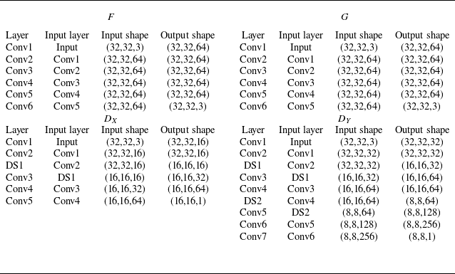
Table 4. Architectures of the CNN models used in cGAN in figure 1. The bottommost layers correspond to the outputs of each model. Here ‘Conv’ refers to two-dimensional convolution layers, ‘DS’ refers to downsampling layers, ‘US’ refers to upsampling layers and ‘Concat’ refers to channelwise concatenation. See § 2.2.1 for nomenclature of each model.
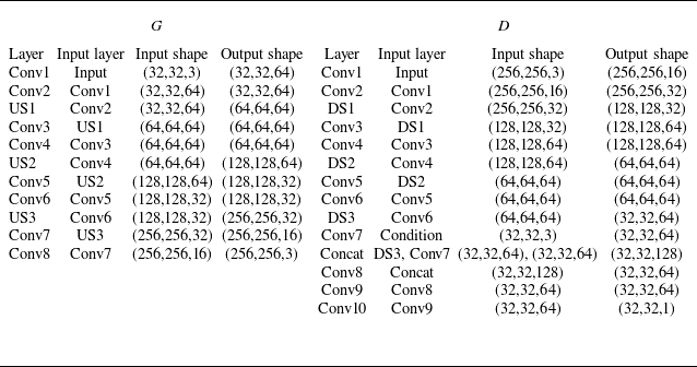
Appendix B. Results for LESx4 at
$\boldsymbol{Re}_{\boldsymbol\tau} \boldsymbol{\approx} \boldsymbol{1000}$

Here, the a priori and a posteriori results for the LESx4 case at $Re_\tau \approx 1000$
are presented. The LESx4 case uses a grid of
$Re_\tau \approx 1000$
are presented. The LESx4 case uses a grid of $ (\Delta x^+, \Delta z^+ ) \approx (36,18)$
that is four times as coarse as the DNS grid as the LESx8 uses an eight-times-coarse grid (
$ (\Delta x^+, \Delta z^+ ) \approx (36,18)$
that is four times as coarse as the DNS grid as the LESx8 uses an eight-times-coarse grid ( $ ( \Delta x^+, \Delta z^+ ) \approx (72,36)$
) as shown in table 1. Therefore, the LESx4 grid is expected to sufficiently resolve the energetic near-wall streak structures of
$ ( \Delta x^+, \Delta z^+ ) \approx (72,36)$
) as shown in table 1. Therefore, the LESx4 grid is expected to sufficiently resolve the energetic near-wall streak structures of $\lambda _z^+ \approx 100$
(Smith & Metzler Reference Smith and Metzler1983) with five to six grid points per wavelength, which is important to the accurate resolution of the near-wall turbulence structures. This grid resolution is close to the the grid resolution requirements for LES of fully developed turbulent boundary layers suggested by Kawai & Fujii (Reference Kawai and Fujii2008).
$\lambda _z^+ \approx 100$
(Smith & Metzler Reference Smith and Metzler1983) with five to six grid points per wavelength, which is important to the accurate resolution of the near-wall turbulence structures. This grid resolution is close to the the grid resolution requirements for LES of fully developed turbulent boundary layers suggested by Kawai & Fujii (Reference Kawai and Fujii2008).
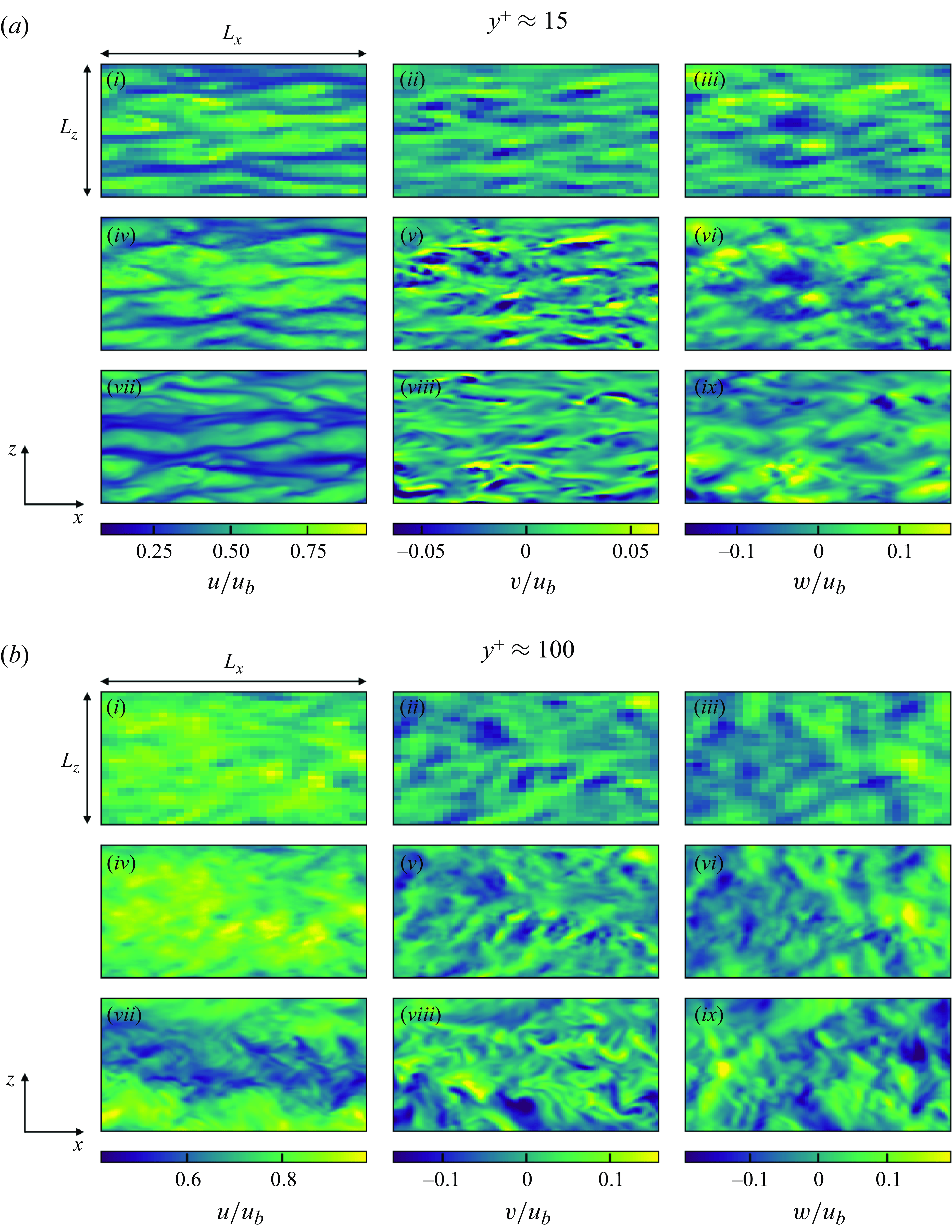
Figure 30. Instantaneous velocity distributions in wall-parallel ( $x$
–
$x$
– $z$
) plane obtained by proposed unsupervised–supervised pipeline with LESx4 at
$z$
) plane obtained by proposed unsupervised–supervised pipeline with LESx4 at $Re_\tau \approx 1000$
. The region corresponds to
$Re_\tau \approx 1000$
. The region corresponds to $(L_x, L_z) = (1.152 \delta , 0.576 \delta )$
. Velocity components are non-dimensionalised by the bulk velocity
$(L_x, L_z) = (1.152 \delta , 0.576 \delta )$
. Velocity components are non-dimensionalised by the bulk velocity $u_b$
. (i,iv,vii) Streamwise component (
$u_b$
. (i,iv,vii) Streamwise component ( $u$
); (ii,v,viii) wall-normal component (
$u$
); (ii,v,viii) wall-normal component ( $v$
); (iii,vi,ix) spanwise component (
$v$
); (iii,vi,ix) spanwise component ( $w$
). (a) Input LESx4; middle, predicted super-resolved flow; (b) reference DNS.
$w$
). (a) Input LESx4; middle, predicted super-resolved flow; (b) reference DNS.
B.1. A priori results
The a priori results of the super-resolution and the predicted SGS stresses of LESx4 are discussed. For brevity, the results of the a priori test using the entire proposed unsupervised–supervised pipeline (figure 15 a) are shown (equivalent to § 5.3 for LESx8).
Figure 30 shows the instantaneous velocity distributions of the predicted super-resolved flow fields at $y^+ \approx 15$
and
$y^+ \approx 15$
and $100$
, and figure 31 shows the instantaneous velocity distributions of the predicted super-resolved flow fields in the streamwise (
$100$
, and figure 31 shows the instantaneous velocity distributions of the predicted super-resolved flow fields in the streamwise ( $y$
–
$y$
– $z$
) cross-sectional plane. As discussed above and in § 4.1, the flow fields obtained by LESx4 sufficiently resolve the near-wall streak structures. The proposed unsupervised–supervised pipeline additionally predicts the smaller turbulent structures that are not present in the input LESx4. It is also notable that minimal changes are made to the eddies that are resolved by LESx4. We stress again that, because the LES and DNS simulations do not match on the level of instantaneous flow fields, the distributions shown in the figure do not correspond on a one-to-one basis. The results suggest that the proposed pipeline does not negatively affect the accurately resolved eddies in sufficiently fine computational grids.
$z$
) cross-sectional plane. As discussed above and in § 4.1, the flow fields obtained by LESx4 sufficiently resolve the near-wall streak structures. The proposed unsupervised–supervised pipeline additionally predicts the smaller turbulent structures that are not present in the input LESx4. It is also notable that minimal changes are made to the eddies that are resolved by LESx4. We stress again that, because the LES and DNS simulations do not match on the level of instantaneous flow fields, the distributions shown in the figure do not correspond on a one-to-one basis. The results suggest that the proposed pipeline does not negatively affect the accurately resolved eddies in sufficiently fine computational grids.
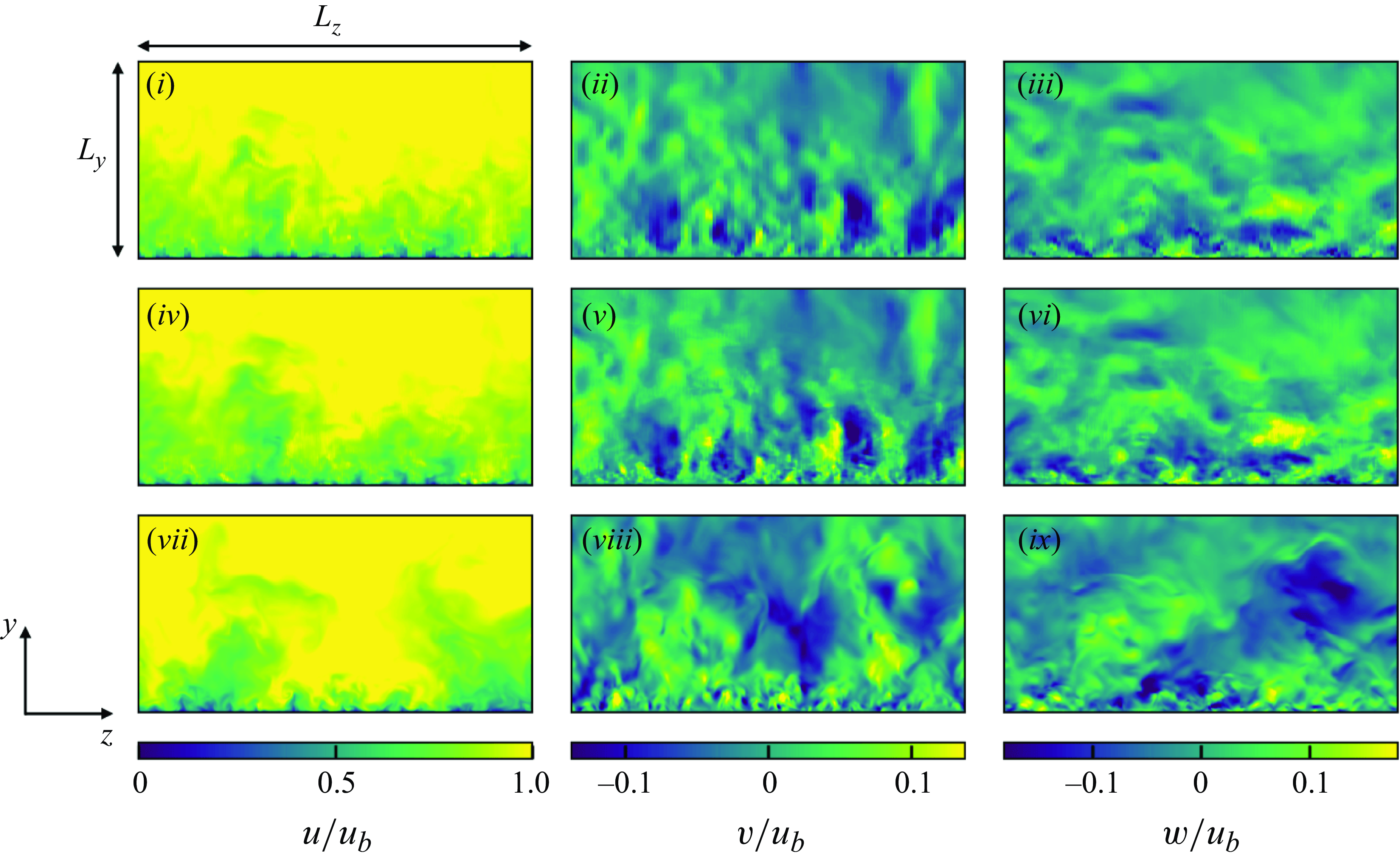
Figure 31. Instantaneous velocity distributions in the streamwise ( $y$
–
$y$
– $z$
) cross-sectional plane for proposed unsupervised–supervised pipeline with LESx4 at
$z$
) cross-sectional plane for proposed unsupervised–supervised pipeline with LESx4 at $Re_\tau \approx 1000$
. The region corresponds to
$Re_\tau \approx 1000$
. The region corresponds to $(L_y, L_z) = (\delta , 2 \delta )$
. Velocity components are non-dimensionalised by the bulk velocity
$(L_y, L_z) = (\delta , 2 \delta )$
. Velocity components are non-dimensionalised by the bulk velocity $u_b$
. (i,iv,vii) Streamwise component (
$u_b$
. (i,iv,vii) Streamwise component ( $u$
); (ii,v,viii) wall-normal component (
$u$
); (ii,v,viii) wall-normal component ( $v$
); (iii,vi,ix) spanwise component (
$v$
); (iii,vi,ix) spanwise component ( $w$
); (i–iii) input LESx4; (iv–vi) predicted super-resolved flow; (vii–ix) reference DNS.
$w$
); (i–iii) input LESx4; (iv–vi) predicted super-resolved flow; (vii–ix) reference DNS.

Figure 32. Streamwise (a,c) and spanwise (b,d) energy spectra of predicted super-resolved velocity fields at $Re_\tau \approx 1000$
. Here (a,b)
$Re_\tau \approx 1000$
. Here (a,b) $y^+ \approx 15$
; (c,d)
$y^+ \approx 15$
; (c,d) $y^+ \approx 100$
. Blue, streamwise component; orange, wall-normal component; green, spanwise component. Solid lines, predicted super-resolved flow using proposed unsupervised–supervised pipeline (figure 15
a); dashed lines, typical supervised model (figure 15
b); circles, reference DNS; pluses, input LESx4.
$y^+ \approx 100$
. Blue, streamwise component; orange, wall-normal component; green, spanwise component. Solid lines, predicted super-resolved flow using proposed unsupervised–supervised pipeline (figure 15
a); dashed lines, typical supervised model (figure 15
b); circles, reference DNS; pluses, input LESx4.
Figure 32 shows the energy spectra of the predicted super-resolved velocity flow fields. The spectra obtained by the proposed unsupervised–supervised pipeline show good agreement with the reference DNS, while the typical supervised model shows some discrepancies, most notably at $y^+ \approx 15$
. Figures 33 and 34 show the turbulence statistics of the predicted flow and the extracted SGS stresses, respectively. The mean streamwise velocity of LESx4 already matches that of the DNS, and neither the proposed pipeline nor the supervised model alters the LESx4 velocity and the results agree with the DNS. In the resolved Reynolds stresses and the extracted SGS stresses, the predictions by the proposed pipeline agree better with the reference profiles compared with the typical supervised method. These observations are qualitatively similar to the LESx8 case discussed in § 2.2.2. These results suggest that the proposed unsupervised learning is effective even for conventional well-resolved LES.
$y^+ \approx 15$
. Figures 33 and 34 show the turbulence statistics of the predicted flow and the extracted SGS stresses, respectively. The mean streamwise velocity of LESx4 already matches that of the DNS, and neither the proposed pipeline nor the supervised model alters the LESx4 velocity and the results agree with the DNS. In the resolved Reynolds stresses and the extracted SGS stresses, the predictions by the proposed pipeline agree better with the reference profiles compared with the typical supervised method. These observations are qualitatively similar to the LESx8 case discussed in § 2.2.2. These results suggest that the proposed unsupervised learning is effective even for conventional well-resolved LES.
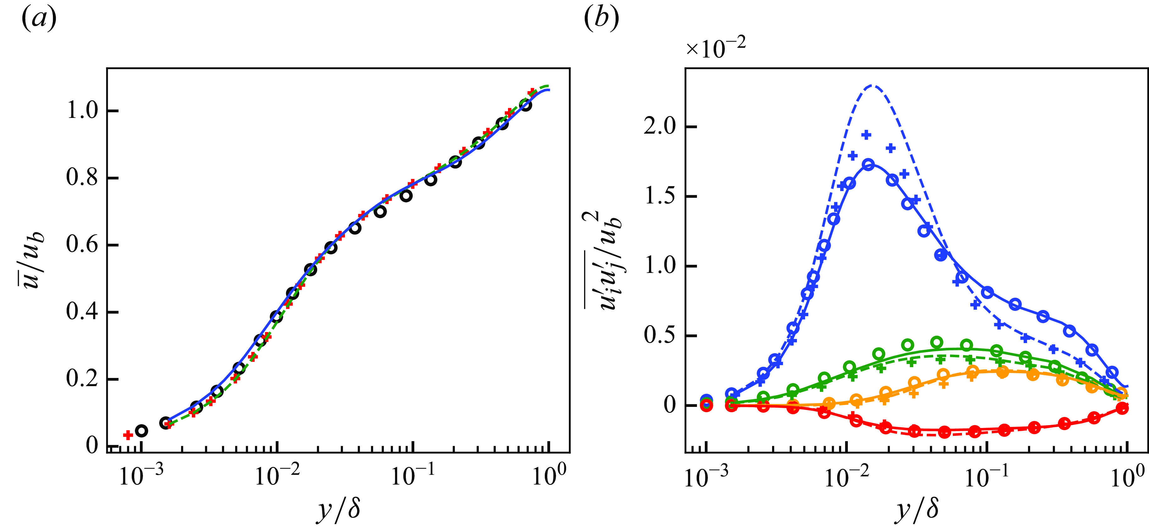
Figure 33. Mean streamwise velocity (a) and resolved reynolds stresses (b) of predicted super-resolved flows at $Re_\tau \approx 1000$
. Solid lines, predicted super-resolved flow using proposed unsupervised–supervised-pipeline SGS model (figure 15
a); dashed lines, typical supervised model (figure 15
b); circles, reference DNS; crosses, input LESx4. For (b): blue, streamwise normal component (
$Re_\tau \approx 1000$
. Solid lines, predicted super-resolved flow using proposed unsupervised–supervised-pipeline SGS model (figure 15
a); dashed lines, typical supervised model (figure 15
b); circles, reference DNS; crosses, input LESx4. For (b): blue, streamwise normal component ( $\overline {u^{\prime}u^{\prime}}$
); orange, wall-normal normal component (
$\overline {u^{\prime}u^{\prime}}$
); orange, wall-normal normal component ( $\overline {v^{\prime}v^{\prime}}$
); green, spanwise normal component (
$\overline {v^{\prime}v^{\prime}}$
); green, spanwise normal component ( $\overline {w^{\prime}w^{\prime}}$
); red, shear component (
$\overline {w^{\prime}w^{\prime}}$
); red, shear component ( $\overline {u^{\prime}v^{\prime}}$
).
$\overline {u^{\prime}v^{\prime}}$
).
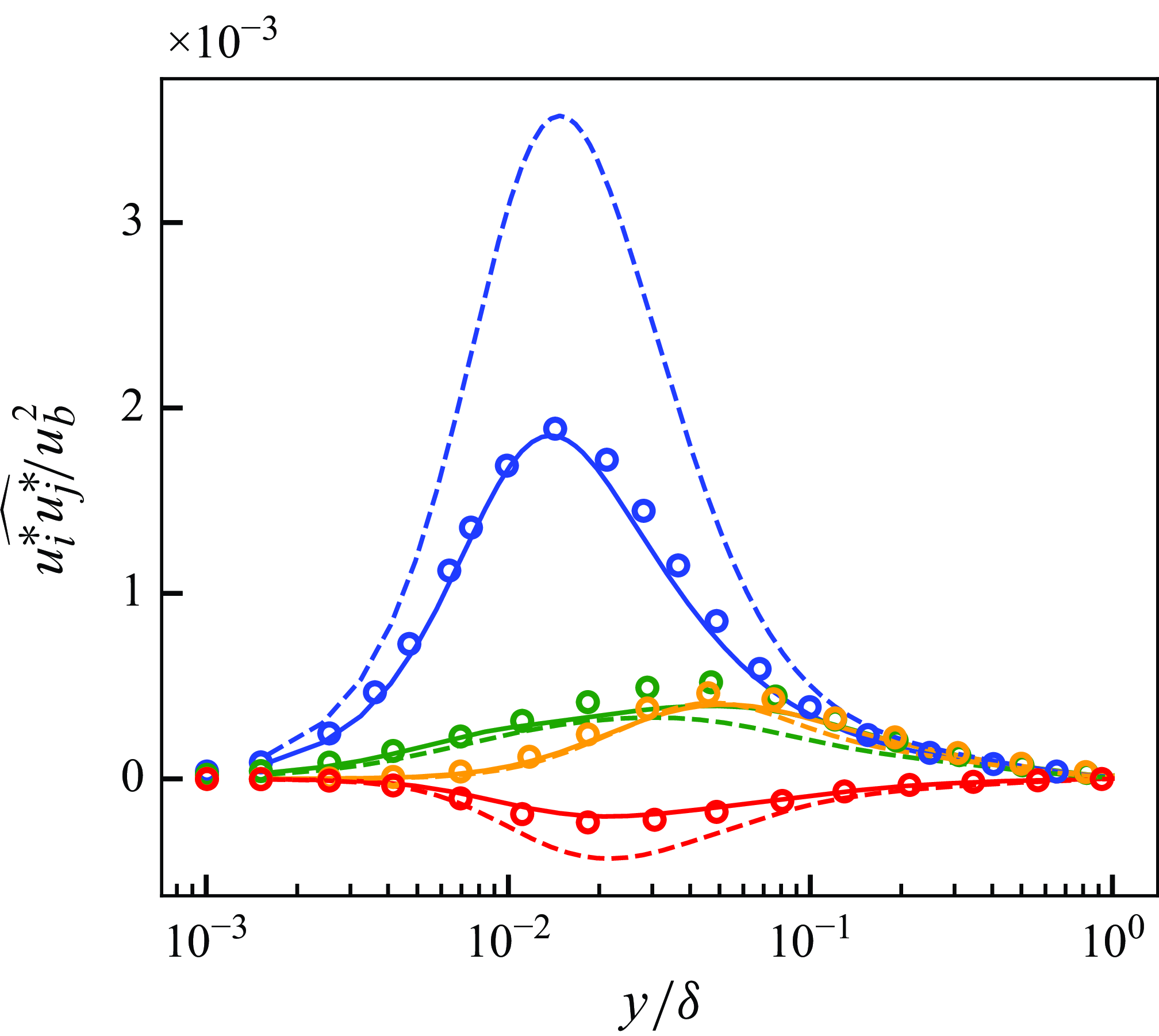
Figure 34. The SGS stresses extracted from predicted super-resolved flows at $Re_\tau \approx 1000$
. Solid lines, predicted super-resolved flow using proposed unsupervised–supervised-pipeline SGS model (figure 15
a); dashed lines, typical supervised model (figure 15
b); circles, reference DNS. Blue, streamwise normal component (
$Re_\tau \approx 1000$
. Solid lines, predicted super-resolved flow using proposed unsupervised–supervised-pipeline SGS model (figure 15
a); dashed lines, typical supervised model (figure 15
b); circles, reference DNS. Blue, streamwise normal component ( $\widehat {u^* u^*}$
); orange, wall-normal normal component (
$\widehat {u^* u^*}$
); orange, wall-normal normal component ( $\widehat {v^* v^*}$
); green, spanwise normal component (
$\widehat {v^* v^*}$
); green, spanwise normal component ( $\widehat {w^* w^*}$
); red, shear component (
$\widehat {w^* w^*}$
); red, shear component ( $\widehat {u^* v^*}$
).
$\widehat {u^* v^*}$
).
B.2. A posteriori results
Here, the turbulence statistics obtained by the a posteriori test at $Re_\tau \approx 1000$
are presented. Figure 35 shows the obtained mean streamwise velocity and the Reynolds shear stress. The proposed unsupervised–supervised-pipeline SGS model shows good agreement in the predicted mean velocity to the reference DNS, while the conventional SGS model shows some discrepancies. Similarly, the proposed model shows good agreement of the near-wall shear stress. Figure 36 shows the components of the Reynolds normal stresses. The proposed model shows differences with the conventional SGS model in the wall-normal and spanwise components while the streamwise component is similar. These observations are qualitatively similar to the observations from the LESx8 case discussed in § 6. The results indicate that the proposed unsupervised–supervised machine-learning pipeline methodology to SGS modelling does not negatively affect the LES predictions for sufficiently fine computational grids and may yield better results compared with conventional SGS models.
$Re_\tau \approx 1000$
are presented. Figure 35 shows the obtained mean streamwise velocity and the Reynolds shear stress. The proposed unsupervised–supervised-pipeline SGS model shows good agreement in the predicted mean velocity to the reference DNS, while the conventional SGS model shows some discrepancies. Similarly, the proposed model shows good agreement of the near-wall shear stress. Figure 36 shows the components of the Reynolds normal stresses. The proposed model shows differences with the conventional SGS model in the wall-normal and spanwise components while the streamwise component is similar. These observations are qualitatively similar to the observations from the LESx8 case discussed in § 6. The results indicate that the proposed unsupervised–supervised machine-learning pipeline methodology to SGS modelling does not negatively affect the LES predictions for sufficiently fine computational grids and may yield better results compared with conventional SGS models.
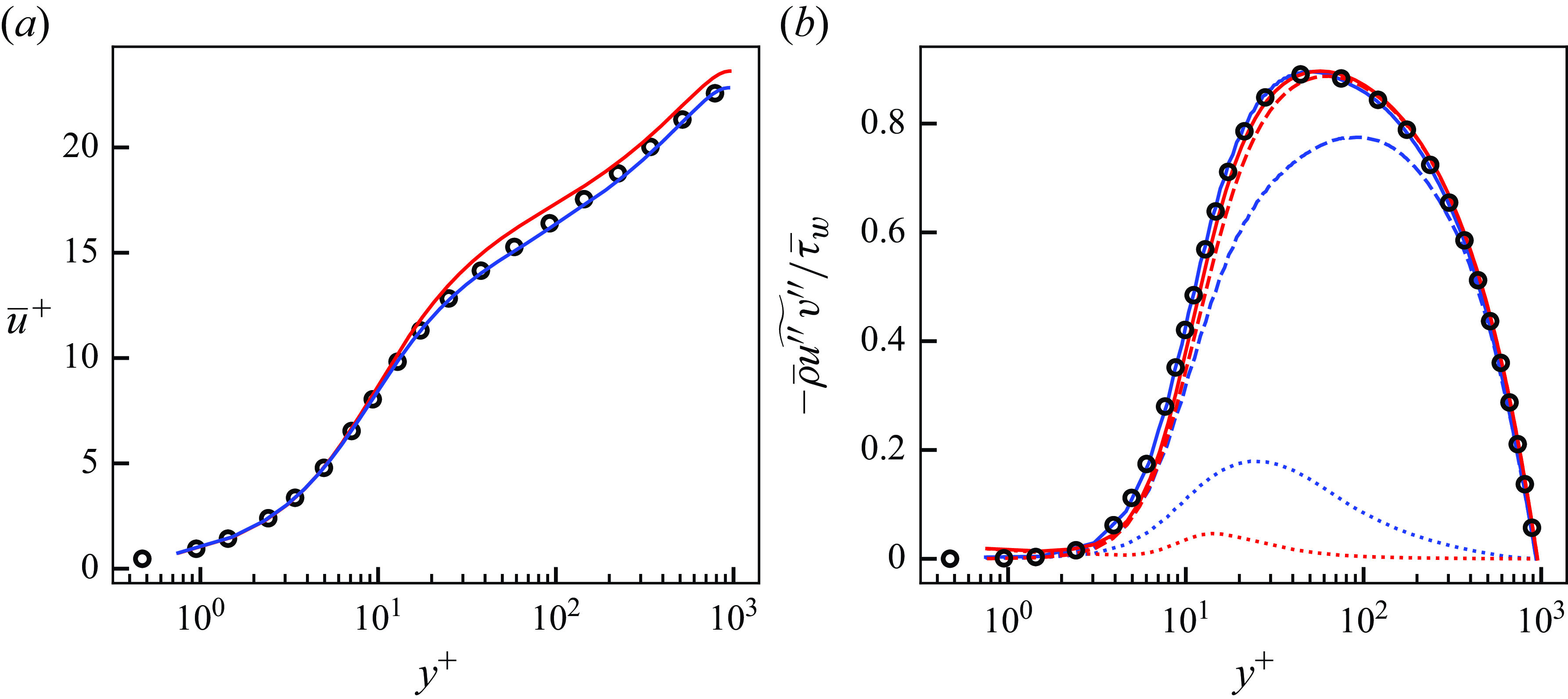
Figure 35. Mean streamwise velocity (a) and Reynolds shear stress (b) of a posteriori tests at $Re_\tau \approx 1000$
. Blue, LESx4 with proposed unsupervised–supervised-pipeline SGS model (figure 15
a); red, LESx4 with typical SGS model; black circles, reference DNS. For (b): dashed lines, resolved component; dotted lines, SGS component; solid lines, resolved + SGS stress.
$Re_\tau \approx 1000$
. Blue, LESx4 with proposed unsupervised–supervised-pipeline SGS model (figure 15
a); red, LESx4 with typical SGS model; black circles, reference DNS. For (b): dashed lines, resolved component; dotted lines, SGS component; solid lines, resolved + SGS stress.
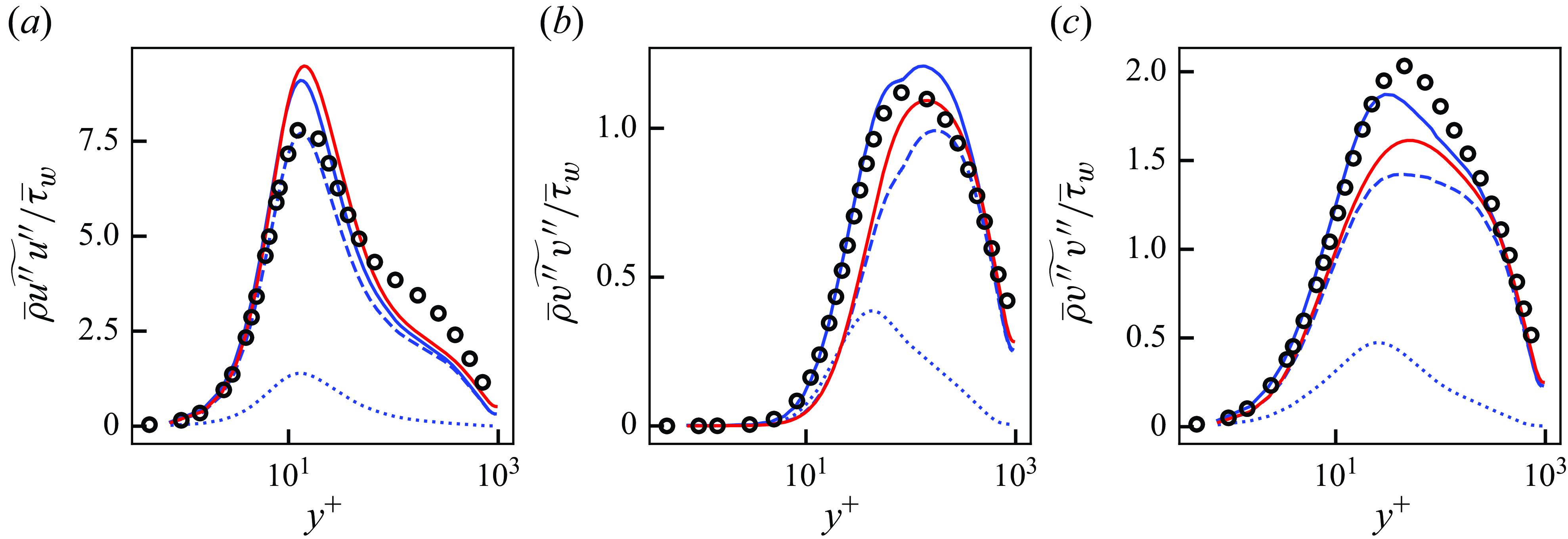
Figure 36. Streamwise (a), wall-normal (b) and spanwise (c) Reynolds stress of a posteriori tests at $Re_\tau \approx 1000$
. Blue, LESx4 with proposed unsupervised–supervised-pipeline SGS model (figure 15
a); red, LESx4 with typical SGS model; black circles, reference DNS. Dashed lines, resolved component; dotted lines, SGS component; solid lines, resolved + SGS stress.
$Re_\tau \approx 1000$
. Blue, LESx4 with proposed unsupervised–supervised-pipeline SGS model (figure 15
a); red, LESx4 with typical SGS model; black circles, reference DNS. Dashed lines, resolved component; dotted lines, SGS component; solid lines, resolved + SGS stress.
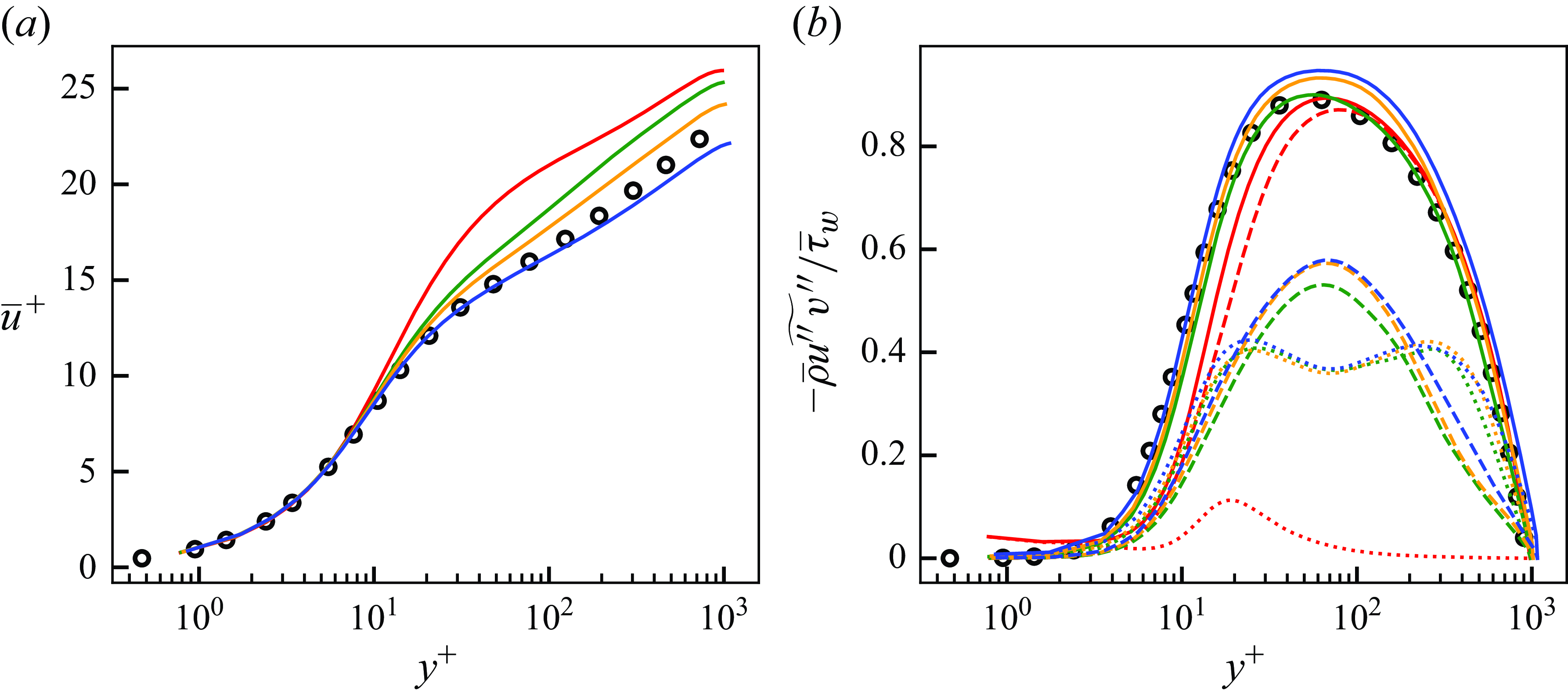
Figure 37. Mean streamwise velocity (a) and Reynolds shear stress (b) of a posteriori tests at $Re_\tau \approx 1000$
. Green,
$Re_\tau \approx 1000$
. Green, $\mu _{\textit{clip}} / \mu _{w} = 0$
; orange,
$\mu _{\textit{clip}} / \mu _{w} = 0$
; orange, $\mu _{\textit{clip}} / \mu _{w} \approx -1$
; blue,
$\mu _{\textit{clip}} / \mu _{w} \approx -1$
; blue, $\mu _{\textit{clip}} / \mu _{w} \approx -2$
; red, vLES with typical SGS model; black circles, reference DNS. For (b): dashed lines, resolved component; dotted lines, SGS component; solid lines, resolved + SGS stress.
$\mu _{\textit{clip}} / \mu _{w} \approx -2$
; red, vLES with typical SGS model; black circles, reference DNS. For (b): dashed lines, resolved component; dotted lines, SGS component; solid lines, resolved + SGS stress.
Appendix C. Effects of the clipping parameter
$\boldsymbol{\mu} _{\textbf{clip}}$

This appendix presents the effects of the clipping parameter $\mu _{\textit{clip}}$
used in (3.2). The a posteriori results using
$\mu _{\textit{clip}}$
used in (3.2). The a posteriori results using $\mu _{\textit{clip}} / \overline {\mu }_w = 0$
and
$\mu _{\textit{clip}} / \overline {\mu }_w = 0$
and $\mu _{\textit{clip}} / \overline {\mu }_w \approx -1$
are shown in addition to
$\mu _{\textit{clip}} / \overline {\mu }_w \approx -1$
are shown in addition to $\mu _{\textit{clip}} / \overline {\mu }_w \approx -2$
that was shown in § 6. As mentioned in § 3.2, a small value of
$\mu _{\textit{clip}} / \overline {\mu }_w \approx -2$
that was shown in § 6. As mentioned in § 3.2, a small value of $\mu _{\textit{clip}}$
yields less clipped backscatter. In the case of
$\mu _{\textit{clip}}$
yields less clipped backscatter. In the case of $\mu _{\textit{clip}} / \overline {\mu }_w = 0$
, the SGS stress only predicts forward scatter of kinetic energy. We note that
$\mu _{\textit{clip}} / \overline {\mu }_w = 0$
, the SGS stress only predicts forward scatter of kinetic energy. We note that $\mu _{\textit{clip}} / \overline {\mu }_w \approx -3$
led to instabilities of the computation and thus not shown.
$\mu _{\textit{clip}} / \overline {\mu }_w \approx -3$
led to instabilities of the computation and thus not shown.
Figure 37 shows the obtained mean streamwise velocity and the Reynolds shear stress. It can be observed that as $\mu _{\textit{clip}}$
decreases, the streamwise velocity approaches the reference DNS profile. The difference in the velocity profiles may be attributed to the weakened SGS backscatter with
$\mu _{\textit{clip}}$
decreases, the streamwise velocity approaches the reference DNS profile. The difference in the velocity profiles may be attributed to the weakened SGS backscatter with $\mu _{\textit{clip}} / \mu _w = 0$
and
$\mu _{\textit{clip}} / \mu _w = 0$
and $\mu _{\textit{clip}} / \mu _w \approx -1$
, as the clipping procedure weakens the production of velocity fluctuations. The result indicates the importance of the SGS backscatter in vLES, and the appropriate prediction of SGS backscatter is crucial to the accurate prediction of the streamwise velocity, as shown in § 6. Therefore, it is desirable to clip as little backscatter as possible by setting
$\mu _{\textit{clip}} / \mu _w \approx -1$
, as the clipping procedure weakens the production of velocity fluctuations. The result indicates the importance of the SGS backscatter in vLES, and the appropriate prediction of SGS backscatter is crucial to the accurate prediction of the streamwise velocity, as shown in § 6. Therefore, it is desirable to clip as little backscatter as possible by setting $\mu _{\textit{clip}}$
as small as possible. Another observation is that
$\mu _{\textit{clip}}$
as small as possible. Another observation is that $\mu _{\textit{clip}} / \overline {\mu }_w = 0$
gives a better prediction of the mean velocity profile compared with the conventional SGS model. While both models do not predict the SGS backscatter of energy, the proposed machine-learning-based SGS model is shown to provide a better prediction for vLES.
$\mu _{\textit{clip}} / \overline {\mu }_w = 0$
gives a better prediction of the mean velocity profile compared with the conventional SGS model. While both models do not predict the SGS backscatter of energy, the proposed machine-learning-based SGS model is shown to provide a better prediction for vLES.
We note that the clipping procedure is necessary for the stable computation of vLES. Matsumoto, Inubushi & Goto (Reference Matsumoto, Inubushi and Goto2024) have shown that machine-learning turbulence models for the computational grids with $k_{\textit{max}} \eta \lt 0.2$
, where
$k_{\textit{max}} \eta \lt 0.2$
, where $k_{\textit{max}}$
is the maximum resolved wavenumber and
$k_{\textit{max}}$
is the maximum resolved wavenumber and $\eta$
is the Kolmogorov length scale, cannot perform stable computation. The spanwise grid resolution in the near-wall region for the present vLES (i.e. LESx8) gives
$\eta$
is the Kolmogorov length scale, cannot perform stable computation. The spanwise grid resolution in the near-wall region for the present vLES (i.e. LESx8) gives $k_{z,{\textit{max}}} \eta \approx 0.13$
(details of the computational grid and the flow condition are shown in § 4), which necessitates the clipping procedure.
$k_{z,{\textit{max}}} \eta \approx 0.13$
(details of the computational grid and the flow condition are shown in § 4), which necessitates the clipping procedure.


 Open access