


1 Introduction
The control of the flow surrounding bluff bodies can greatly improve their aerodynamic performance. A rich body of literature describes this topic, mainly due to the vast number of applications in the engineering sciences. Typical examples of such applications include flows past transportation vehicles, from submarines to airplanes. In all these cases, the Reynolds number ( $Re$) exceeds a critical value and, when this happens, phenomena such as vortex shedding occur, characterizing the formation of a turbulent wake associated with a low base pressure level. The vortex shedding, however, is not the only phenomenon associated with bluff-body flows. Another critical event is the presence of separation and reattachment of boundary layers (BLs) on the model’s surface. This phenomenon usually originates at the leading edge of blunt bodies where the flow is forced to separate (with different level of severity) by a sharp or a rounded edge. Researchers have widely investigated rectangular ( $r/D=0$) and circular ( $r/D=0.5$; so-called D-shaped body (Pastoor et al. Reference Pastoor, Henning, Noack, King and Tadmor2008; Han, Krajnović & Basara Reference Han, Krajnović and Basara2013)) cylinders representing the two extremes of the ratio between the radius of the leading edges $r$ and the characteristic dimension of the cylinder $D$ (see figure 1). In the first case, the separation is forced and triggered by sharp edges, while, in the second case, the flow remains attached to the surface, making the square back separation at the rear end of the body the dominant feature characterizing its aerodynamic performance. Less attention has been paid to rectangular cylinders with lightly rounded leading edges, where the separation of the flow is induced by a strong adverse pressure gradient at the leading edge. Depending on the length of the body, this shear layer may reattach on the model surface or merge with the wake flow. The presence of a lightly rounded leading edge makes the bluff body of relevant interest for applications related to ground vehicle transportation, where, for example, modern buses and trucks are characterized by filleted corners. At the same time, the simplification of a vehicle into a cylinder allows one to investigate in depth important physical behaviours, otherwise hindered by the complexity of added details.

Figure 1. Cross-sections of cylinders of relevant importance: (a) square, (b) circular and (c) lightly rounded leading-edge cylinders.
The description and control of the flow around cylinders or bodies of revolution has mainly focused on either the leading-edge or the rear-end separation, the former using  $r/D=0$ shapes and the latter using fully rounded D-shaped bodies. The work performed by Sigurdson (Reference Sigurdson1995) demonstrated experimentally the possibility of effective control when actuating the flow at the sharp leading edge of a bluff body. It also showed a strong relation between the recirculation bubble height and the drag experienced by the body. Another interesting work on bodies of revolution with sharp edges (Higuchi et al. Reference Higuchi, van Langen, Sawada and Tinney2006; Higuchi, Sawada & Kato Reference Higuchi, Sawada and Kato2008) indicated the presence of an optimal length-to-diameter ratio for the lowest drag. In Higuchi et al. (Reference Higuchi, Sawada and Kato2008), it is shown that the lowest drag is obtained when the separated flow reattaches just before the rear end of the body. The work of Higuchi et al. (Reference Higuchi, Sawada and Kato2008) points to the necessity of a global approach, in which the effect of the front separation on the wake is taken into consideration. Thus, the present work should shed light on a topic missing in the literature, i.e. the study of the interaction between the front and the rear separations of bluff bodies. In particular, this is achieved by the manipulation of the leading-edge shear flow, in order to control both the local separation (at the side of the body) and the downstream wake dynamics, reducing the global drag and improving the lateral stability. This may have a strong impact on real-life applications. An enhanced stability significantly improves the safety of ground vehicles, and a large drag reduction (larger than 10 %) can have enormous benefit on the economy of a truck fleet, where two-thirds of the total operating cost comes from fuel/energy consumption. In this work, it is reported, for the optimal case, a 20 % drag reduction and a significant decrease of the side force fluctuations.
Control strategies have historically been divided into three main groups (Gad-el Hak Reference Gad-el Hak2007; Choi, Jeon & Kim Reference Choi, Jeon and Kim2008): passive, active open-loop and active closed-loop controls. The last differs from open-loop control by the presence of feedback sensors. Moreover, in Choi et al. (Reference Choi, Jeon and Kim2008), a clear distinction between BL control and direct-wake control has been described. The first deals with bluff bodies with a movable separation point, and the second describes cases where the control directly affects the wake structures. This distinction, however, is not suitable for the present study, where an apparent BL control (placed at the front rounded leading edge) will indirectly affect the downstream structures, penetrating into the wake and defining, to some extent, its dynamics. For this purpose, an optimization of the actuation parameters governed by a genetic algorithm (GA) is proposed. The optimization algorithm is readapted for a flow control application, following the guidelines given by Wahde (Reference Wahde2008), where genetically inspired techniques are elucidated. Similarly, a previous experimental work (Li et al. Reference Li, Noack, Cordier, Borée and Harambat2017) had also used a GA-based optimization for the direct-wake control of an Ahmed body, showing impressive results in terms of drag reduction. In the same work, the importance of a multi-frequency control was also shown, which inspired the form of the control law selected for the present work. In contrast to the work of Li et al. (Reference Li, Noack, Cordier, Borée and Harambat2017), the present study aims to identify a viable way to control the wake only by intervention on the upstream leading-edge BL. This technique is in addition expected to use a lower energy level to manipulate a BL characterized by a low turbulence level. A recent study also reported on the role of free-stream turbulence (FST) (Lander et al. Reference Lander, Letchford, Amitay and Kopp2016), showing that an increased FST level affects not only the early leading-edge separation but also the entire wake dynamics. Therefore, by introducing a disturbance into the upstream flow, it is possible to greatly affect the wake, using a limited amount of energy for the actuation.
The present paper is organized as follows. In § 2 the methodology and the domain used for the computational fluid dynamics (CFD) simulations are given. A description of the GA is also reported. In § 3 the results are discussed, focusing first on the GA procedure. Secondly, a deeper flow analysis of the unactuated and controlled case is reported. The last part of § 3 is dedicated to the comparison of the present GA-controlled case versus the use of previously published control strategy guidelines for a similar case (Minelli et al. Reference Minelli, Krajnović, Basara and Noack2016, Reference Minelli, Adi Hartono, Chernoray, Hjelm, Krajnović and Basara2017b). Conclusions follow in § 4.
2 Methodology and numerical set-up
Large-eddy simulations (LES) at  $Re=40\,000$ are used to predict the flow field in both two-dimensional (2-D) and three-dimensional (3-D) modes. As mentioned in the introduction, this study is divided into two parts. The first one uses the drag obtained from 2-D unsteady simulations as the objective function in a genetic optimization algorithm. The use of 2-D simulations is justified by the enormous numerical resources that the GA process would have taken with 3-D simulations, and by the fact that the use of a homogeneous actuation along the $z$ direction somehow forces the flow towards a 2-D-like separation also in 3-D cases. This last point and the description of the similarities between the 2-D and 3-D cases is part of the result section and will be shown later. The second part of the paper adopts the best control law (in terms of $C_{d}$ reduction) found by the 2-D GA process, for a 3-D simulation of a bluff-body flow control application. The authors are aware of the errors introduced by turbulent 2-D simulations, but they also consider this step necessary to gather important control law information, the consistency of which is verified at a later stage using well-resolved 3-D LES. Overall, the use of 2-D simulations not only accelerates the process towards an optimal control law but also highlights the two-dimensionalization effect of the present flow control on a 3-D turbulent flow.
The 2-D and 3-D numerical domains are presented in figure 2(a) and 2(c), respectively. For both simulation modes, a homogeneous Neumann boundary condition (BC) is applied at the outlet, while a constant velocity is set at the inlet to drive the flow. The lateral walls are set to symmetry. Only for the 3-D simulations, the top and bottom surfaces are periodic BCs reproducing an infinitely extruded bluff body. The flow is sampled in both 2-D and 3-D modes. A 2-D plane, figure 2(b), is used in the first case, while a corresponding 3-D volume is sampled in the second case, figure 2(d). All dimensions in figure 2 refer to the characteristic dimension of the main geometry  $D$, the width (and length) of the model. The front rounded corners of the bluff body have a radius $r=0.05D$. These rounded edges force the flow (in the unactuated case) to separate due to the adverse pressure gradient imposed by the curvature. At the centre of the curvature, a time-varying velocity BC is set for the slot’s width $G=0.0025D$. This corresponds to a $2.8^{\circ }$ width centred around the middle of the curvature ( $\unicode[STIX]{x1D6FD}$ in figure 2b). The choice of the active flow control (AFC) positioning is supported by previous work performed by the authors. In particular, in Minelli et al. (Reference Minelli, Tokarev, Zhang, Liu, Chernoray, Basara and Krajnović2019) the sensitivity of the positioning of the jet slot is described. In the latter work, it is shown that the control performed at its best when positioned very close to the separation point of the front curvature, being in this case at $45^{\circ }$ with respect to the streamwise direction. The slot width was chosen to be the same as used in previous works carried out by the authors (Minelli et al. Reference Minelli, Krajnović, Basara and Noack2016, Reference Minelli, Adi Hartono, Chernoray, Hjelm and Krajnović2017a). In the 3-D extruded case, this BC is also defined homogeneously along the $z$ direction. When the flow is unactuated, the AFC surface is defined as a no-slip wall, like the rest of the body. The simulations are made with a cell-centred finite volume method in the commercial software STAR-CCM $+$, in its release 13.06.11 (STAR-CCM+ 2018).
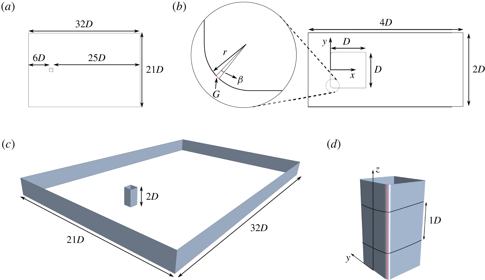
Figure 2. The 2-D and 3-D domains used for the LES. (a) The 2-D domain. (b) A zoom of the sampling 2-D area and the curvature of the front rounded edge. (c) The 3-D domain. (d) A zoom of the 3-D extruded body. A 3-D volume of  $1D$ height is sampled throughout the simulation; the other two dimensions of the sampling volume are kept as in (b).
2.1 Resolution and numerical schemes
The mesh resolution respects the LES indications given by Piomelli & Chasnov (Reference Piomelli, Chasnov, Henningson, Hallbaeck, Alfreddson and Johansson1996) and Pope (Reference Pope2001). In particular, the wall-normal non-dimensional distance of the first grid point is located at  $n^{+}<1$, where $n^{+}=u_{\unicode[STIX]{x1D70F}}n/\unicode[STIX]{x1D708}$, with the friction velocity $u_{\unicode[STIX]{x1D70F}}$. The resolutions in the spanwise ( $z$ and $y$) directions and streamwise ( $x$) direction must further be $\unicode[STIX]{x0394}l^{+}\simeq 15{-}40$ and $\unicode[STIX]{x0394}s^{+}\simeq 50{-}150$, respectively (Piomelli & Chasnov Reference Piomelli, Chasnov, Henningson, Hallbaeck, Alfreddson and Johansson1996). Here, $\unicode[STIX]{x0394}l^{+}=u_{\unicode[STIX]{x1D70F}}\unicode[STIX]{x0394}l/\unicode[STIX]{x1D708}$ and $\unicode[STIX]{x0394}s^{+}=u_{\unicode[STIX]{x1D70F}}\unicode[STIX]{x0394}s/\unicode[STIX]{x1D708}$. In the current simulations, the grid resolution has a maximum value in the wall-normal direction of $n_{max}^{+}=0.8$. The maximum resolutions in the spanwise and streamwise directions are $\unicode[STIX]{x0394}l_{max}^{+}=35$ and $\unicode[STIX]{x0394}l_{max}^{+}=35$, respectively. Although the resolution respects the good-practice LES values, a grid independence study is used to verify the influence of the mesh on the results (see § 3.3.1). The chosen time step, $\unicode[STIX]{x0394}t^{\ast }=\unicode[STIX]{x0394}tU_{\infty }/D$, is $\unicode[STIX]{x0394}t^{\ast }=6\times 10^{-3}$ for all simulations, resulting in a Courant–Friedrichs–Lewy (CFL) number less than 1 in the entire domain. All simulations were run first until the flow was fully developed $t_{dev}^{\ast }=t_{dev}U_{\infty }/D=30$. This was followed by an averaging of $t^{\ast }=tU_{\infty }/D=180$. The convective fluxes are approximated by a blend of 95 % linear interpolation of second-order accuracy (central differencing scheme) and of 5 % upwind differences of first-order accuracy (upwind scheme). The time marching procedure is done using the implicit second-order-accurate, three-time-level scheme. In the current LES, the unresolved small turbulent scales are modelled using the wall-adapting local-eddy viscosity (WALE) subgrid-scale model (Nicoud & Ducros Reference Nicoud and Ducros1999). The mesh is formed by hexahedral units and the grid topology is constructed using a block mesh and the O-grid technique in order to concentrate most of the computational cells close to the body.
2.2 The actuation strategy
As represented in figures 2(b) and 3, the actuators that reproduce a synthetic jet behaviour are located at the centre of the two front rounded corners. The velocity BC given at this location is defined by a multi-frequency signal of the following form:
 $$\begin{eqnarray}U_{afc}=A_{1}\sin (\,f_{1}t2\unicode[STIX]{x03C0})+A_{2}\sin (\,f_{2}t2\unicode[STIX]{x03C0}),\end{eqnarray}$$
 allowing the generation of a sinusoidal wave sketched in figure 3(b). The right and left actuators are always assigned with an in-phase signal, and the corresponding four non-dimensional variables in  $U_{afc}$ ( $A_{1,2}^{+}=A_{1,2}/U_{\infty }$ and $F_{1,2}^{+}=f_{1,2}D/U_{\infty }$) are defined by the GA optimization and they are limited to the following ranges:
 $$\begin{eqnarray}0\leqslant A_{1,2}^{+}\leqslant 1,\quad 0\leqslant F_{1,2}^{+}\leqslant 10.\end{eqnarray}$$
 The ranges represent the search space in which the GA will search for the optimal control law. For clarity, the maximum value that the signal can assume instantly in time is when  $A_{1}^{+}=A_{2}^{+}=1$, being $U_{afc}=2U_{\infty }$. This leads to a maximum ratio of jet to undisturbed velocity of $R_{max}=U_{afc}/U_{\infty }=2$.
The performance of the actuator is described by the momentum coefficient  $C_{\unicode[STIX]{x1D702}}$. This is an indicator of the energy spent for the actuation ( $\bar{I}_{j}$) with respect to the energy of the unactuated flow:
 $$\begin{eqnarray}\displaystyle & \displaystyle \bar{I}_{j}=\left(\frac{2}{T}\right)\unicode[STIX]{x1D70C}_{j}G\int _{0}^{T/2}U_{afc}^{2}(t)\,\text{d}t, & \displaystyle\end{eqnarray}$$
 $$\begin{eqnarray}\displaystyle & \displaystyle C_{\unicode[STIX]{x1D702}}=\frac{\bar{I}_{j}}{{\textstyle \frac{1}{2}}\unicode[STIX]{x1D70C}DU_{\infty }^{2}}. & \displaystyle\end{eqnarray}$$
 Here,  $\unicode[STIX]{x1D70C}_{j}=\unicode[STIX]{x1D70C}$ is the flow density and $T$ is the actuation period. The maximum value that the control can assume is $C_{\unicode[STIX]{x1D702}\,max}=1\times 10^{-2}$. Increasing $C_{\unicode[STIX]{x1D702}}$ is not always beneficial for drag reduction and, as will be described later, the best selected signal results in a relatively low value $C_{\unicode[STIX]{x1D702}\,best}=2.25\times 10^{-4}$. This control is expected to interact with the incoming external flow, actively changing the flow topology and reducing the drag value. Considering figure 3(a), there are two main areas that influence the drag value: the side recirculation and the wake. Previous numerical and experimental studies (Minelli et al. Reference Minelli, Adi Hartono, Chernoray, Hjelm and Krajnović2017a,Reference Minelli, Adi Hartono, Chernoray, Hjelm, Krajnović and Basarab; Minelli, Krajnović & Basara Reference Minelli, Krajnović and Basara2018) showed that the suppression of the side recirculation bubble could significantly reduce the drag on such a bluff body, but it is not clear whether this strategy is optimal to obtain the best global drag reduction and to control the wake dynamics. Only a few recent studies have shown the influence of an upstream control on the wake of a bluff body (Feng & Wang Reference Feng and Wang2014a,Reference Feng and Wangb; Qu et al. Reference Qu, Wang, Feng and He2019). However, compared to the present work, a relatively low $Re$, spanning from 800 to 1000, was used. In addition, a much larger momentum coefficient ( $C_{\unicode[STIX]{x1D702}}=0.022{-}1.25$) was used to characterize the actuators and manipulate the flow field of circular or square cylinders. Therefore, it is still not known whether a low-momentum-coefficient actuation at high $Re$ can affect the wake flow of a bluff body with rounded leading edges. For this reason, the objective function of the optimization process only considers the drag reduction, discarding the direct effect on the side recirculation, letting the control generate the most suitable virtual aeroshaping effect.
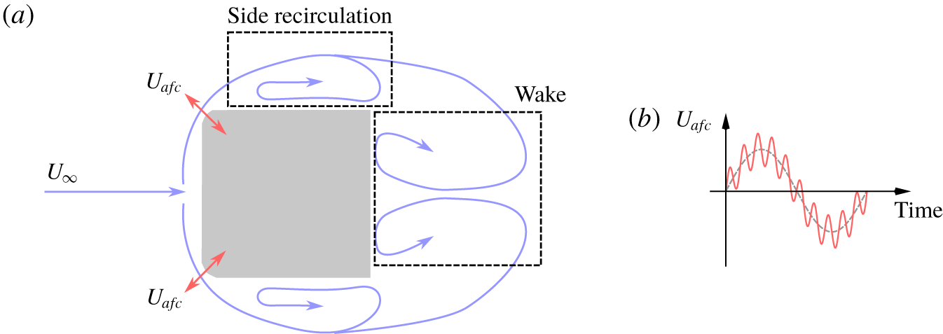
Figure 3. The actuation strategy. (a) A sketch of the flow topology and the actuator location. (b) An example of the actuation signal defined by two frequencies.
2.3 The genetic algorithm optimization
Taking inspiration from the book by Wahde (Reference Wahde2008), a GA optimization was integrated and coupled with the CFD software, as sketched in figure 4. The control is designed in such a way as to resolve a regression problem. In particular, an optimal control law is designed through the minimization process of a cost function. In the present case, the cost function is represented by the averaged  $C_{d}$ value ( $\overline{C_{d}}$) of each simulation. For clarity, $C_{d}$ is averaged over a period $t^{\ast }=180$ and the control parameters (amplitudes and frequencies) are kept constant during one single CFD simulation. Therefore, lower averaged $C_{d}$ values are represented by higher fitness control signals. As represented in figure 4, after a random initialization of the first generation of control signals, the actuation is simulated using the CFD software, and later evaluated by the GA script. At this stage, when all control laws (of the current generation) have been simulated and evaluated, standard GA operations (elitism, cross-over and mutation) are performed. This process generates a new generation of control signals, which are subsequently simulated. The GA parameters are collected in table 1 for simplicity. The GA is based on a binary encoding scheme as originally proposed in Holland (Reference Holland1992). Thus, when the first generation is initialized, a random sequence of binary (0 and 1) values is generated and $B$ (table 1) reads how many bits define each of the four variables. For more details, the reader is referred to § 3 in Wahde (Reference Wahde2008), where the meaning and construction of the parameters is extensively explained. The authors are aware of alternative optimization methods – for example, coupling downhill simplex iteration for the exploitation and Latin hypercube sampling for the exploration (Li et al. Reference Li, Cui, Jia, Li, Yang and Noack2019) – but have chosen the GA optimization for its simplicity and to retain a comparison study with alternative tools as a future work.
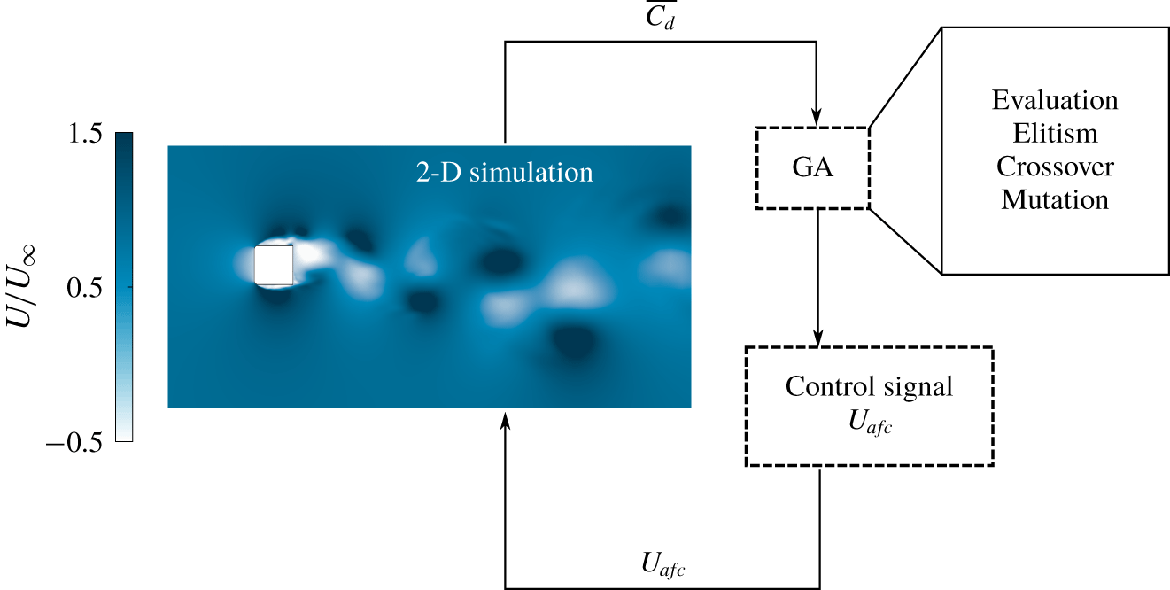
Figure 4. The genetic algorithm optimization work flow.
Table 1. The parameters used in the GA.

3 Results
First, the evolution of the cost function ( $\overline{C_{d}}$) and the outcome from the evolution process is presented. At a later stage, the 2-D flow topology is described and a comparison between unactuated and the lowest drag-actuated case is given. A comparison between the 2-D and 3-D LES is shown, highlighting the conservation of the main flow features from 2-D to 3-D, once the flow is controlled homogeneously along the extrusion direction. Lastly, a comparison between a GA-driven actuation strategy and a previously published control strategy for a similar case is made.
3.1 The genetic algorithm evolution
Figure 5 shows the cost history through the GA optimization. There,  $i$ (abscissa axis) indicates the numbering of each simulated actuation signal, ranked from the lowest to the highest drag value (within one single generation). Each solid line in figure 5 represents one generation, which evolves from the first (
 , green) to the last (
 , yellow). For clarity, a symbol every fifth actuation signal is placed along every generation line. The red dashed line (– – –, red) indicates the $C_{d}$ value of the unforced 2-D case, which corresponds well to classical results presented in the literature (Hoerner Reference Hoerner1965). The first noticeable achievement is the large drag reduction brought about by the multi-frequency control. For this 2-D case, a drag reduction at almost 50 % is observed, resembling the drag reduction achievable by an extreme rounding of the front corners (Hoerner Reference Hoerner1965). A deeper comparison of the flow topologies will be addressed in the following section. Looking at the behaviour of the GA process, one can observe that exploration and exploitation are preserved during the optimization. Specifically, one can notice the following: (i) The first generation (
 , green) already contains drastically lower values of drag compared to the baseline (– – –, red). (ii) After the $20$th generation, only small absolute drag reductions are observed, indicating a good exploitation of the minimum drag value. (iii) The mutation probability coefficient still guarantees a good level of exploration in the search space. The good level of exploration is in fact indicated by a large range of $C_{d}$ values within each and every generation. (iv) The overlapping of the last four lines (from generation 20 to generation 35) can be taken as a good convergence indicator. The case that gives the lowest $C_{d}$ value is therefore selected for further investigation and comparisons.

Figure 5. The evolution cost of the GA optimization procedure. Each line connects the individual  $i$ of each generation from the lowest to the highest ranked. Dashed line (– – –, red) indicates the $C_{d}$ of the unactuated case; (
 , green) connects the individuals of the first generation; (
 , yellow) connects the individuals of the last generation. Sixty individuals were simulated for each of the 35 generations.
Considering the control laws generated by the GA process, one can analyse the trends of the control variables. By the use of multi-dimensional scaling (MDS) (Mardia, Kent & Bibby Reference Mardia, Kent and Bibby1979), one can visualize high-dimensional data in a low-dimensional feature space. The purpose is to define a distance matrix  $C$ able to quantify the relative difference between control laws. If one considers $U_{afc,l}(t)=c_{l}(t)$ and $U_{afc,m}=c_{m}(t)$ as the control laws associated with the $l$th and $m$th individual, it is possible to calculate the difference $C(l,m)$ between two generic control laws as
 $$\begin{eqnarray}C(l,m)=\unicode[STIX]{x1D6FC}\sqrt{\langle |c_{l}(t)-c_{m}(t)|^{2}\rangle }+|J_{l}-J_{m}|.\end{eqnarray}$$
 Here, the first term is the average difference between two control signals, while the second is a penalization based on the cost  $J$. The parameter $\unicode[STIX]{x1D6FC}$ is chosen to impose the maximum variation of the first and second terms equal. The reader is referred to Duriez, Brunton & Noack (Reference Duriez, Brunton and Noack2017) for further details.
Figure 6 shows a proximity map of the control laws (for clarity, only the individuals of every fifth generation are shown). Each dot represents a control law, in a 2-D plane ( $\unicode[STIX]{x1D713}_{1},\unicode[STIX]{x1D713}_{2}$) and the scatterplot is coloured by the cost, which in this case is the $C_{d}$ value. For clarity, the variables $\unicode[STIX]{x1D713}_{1}$ and $\unicode[STIX]{x1D713}_{2}$ are feature coordinates corresponding to the eigenvectors associated with the largest eigenvalues of the distance matrix $C$ populated by the generic terms
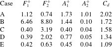
  $C(l,m)$. The individuals draw a parabolic curve with the exception of fewer control laws due to the continued exploration of the GA optimization. Control laws from A to E show the evolution of the control parameters along the drawn parabolic curve and the optimal control law is identified by individual E. Table 2 lists the variables defining each of the selected five control laws on the parabolic curve, and their respective $C_{d}$ values. The primary actuation frequency, $F_{1}^{+}$, evolves from high to low values and stabilizes around the second harmonic of the vortex shedding frequency, reducing progressively its related amplitude $A_{1}^{+}$. Cases C–E do not show significant changes in the $F_{1}^{+}$ and $A_{1}^{+}$ values, the main drag reduction effect being due to the secondary frequency $F_{2}^{+}$. In particular, considering cases C–E, where the primary frequency does not change significantly, one can still observe an important drag reduction related to the secondary frequency change. Comparing cases C and E, one can clearly observe the influence of $F_{2}^{+}$, where, even though $A_{2}^{+}$ remains small, the decrease of the secondary frequency brings a substantial drag reduction. In the optimal case E, $F_{2}^{+}$ is chosen as the third superharmonic of the vortex shedding frequency. A deeper analysis of the flow behaviour of the optimal compared to the non-actuated case is provided in the next section.

Figure 6. Visualization of the 2-D proximity map of the control laws. Only every fifth generation is plotted for clarity. The red circles indicate the five representative cases A–E whose details are listed in table 2. Each dot represents a control law, and the distance between dots is a measure of the difference between two control laws. The colour scheme represents the  $C_{d}$ value.
Table 2. Parameters and  $C_{d}$ values of the five representative cases highlighted in figure 6.
3.2 The 2-D flow topology and the effect of the actuation
Looking at the average streamwise velocity field visualized in figure 7, one can observe a significant change in the distribution of streamlines, in the velocity field intensity and, most importantly, in the topology of the side recirculation and wake regions. The effect of the actuation has a strong global impact on the flow but it does not strongly affect the height and length of the side recirculation bubble. Previous research (Minelli et al. Reference Minelli, Krajnović, Basara and Noack2016, Reference Minelli, Krajnović and Basara2018), on a similar flow control case, focused (probably too intensively) on the suppression of the side recirculation. Even though drag was effectively reduced, the present strategy shows that a global approach to drag reduction results in a more effective control. In the present case, only the averaged  $C_{d}$ is fed back in the control, discarding information on the flow topology (e.g. the size of the side bubble).
Therefore, two important aspects arise from this study. The first one is that the suppression of the side region is not the key factor to reach the highest drag reduction result. The second aspect is that a small disturbance (the control signal) introduced at the incipient pressure-induced separation point can significantly characterize the wake flow. The latter aspect is particularly important for the energy consumption introduced by the control device, as measured by the momentum coefficient  $C_{\unicode[STIX]{x1D702}}$. In fact, the low turbulence level characterizing the attached BL upstream of the flow separation is easier to manipulate, in contrast to a highly turbulent flow (as the detaching shear layer from the trailing edge of the body), which requires a higher energy control to be manipulated. In this regard, one can notice that $C_{\unicode[STIX]{x1D702}}$ is from one to two orders of magnitude lower compared to flow control studies where the control device is directly placed at the base region of a bluff body. This is confirmed by both low- and high- $Re$ studies.
Starting from comparable  $Re$ cases, Pastoor et al. (Reference Pastoor, Henning, Noack, King and Tadmor2008) showed a direct-wake control for a D-shaped body, achieving 15 % drag reduction using $C_{\unicode[STIX]{x1D702}}>0.005$ ( $23\,000<Re<70\,000$). The same behaviour was confirmed by Parkin, Thompson & Sheridan (Reference Parkin, Thompson and Sheridan2013), Parkin, Sheridan & Thompson (Reference Parkin, Sheridan and Thompson2015). These authors state that ‘In any case, actuation at $C_{\unicode[STIX]{x1D702}}=0.004$ seems the appropriate level for peak drag reduction at highest efficiency’ (Parkin et al. Reference Parkin, Thompson and Sheridan2013). A study of a D-shaped cylinder wake was presented by Han et al. (Reference Han, Krajnović and Basara2013) and later by Gao et al. (Reference Gao, Li, Bai and Wu2016) using a $C_{\unicode[STIX]{x1D702}}$ of 3 % and 1 %, respectively, achieving 15 % drag reduction. In addition, Dalla Longa, Morgans & Dahan (Reference Dalla Longa, Morgans and Dahan2017) recently proposed a low-Reynolds-number ( $Re=10\,000$) study of a D-shaped body, showing the use of a comparably low (but still higher than the present study and at a four times lower $Re$) momentum coefficient. In addition, in Dalla Longa et al. (Reference Dalla Longa, Morgans and Dahan2017) the momentum coefficient was set to low values only after a high momentum coefficient stabilized the wake. Considering higher- $Re$ applications, the momentum coefficient reaches values up to two order of magnitude larger than the one used in the present study (Barros et al. Reference Barros, Borée, Noack, Spohn and Ruiz2016; Lambert, Vukasinovic & Glezer Reference Lambert, Vukasinovic and Glezer2016; Li et al. Reference Li, Noack, Cordier, Borée and Harambat2017; Lambert, Vukasinovic & Glezer Reference Lambert, Vukasinovic and Glezer2018; Li et al. Reference Li, Cui, Jia, Li, Yang and Noack2019). In the literature, there also appear a series of bluff-body flow control studies at a much lower $Re=800{-}1200$ (Qu et al. Reference Qu, Wang, Sun, Feng, Pan, Gao and He2017; Ma & Feng Reference Ma and Feng2019). It is noteworthy to observe that those authors utilized a much larger $C_{\unicode[STIX]{x1D702}}=0.007{-}0.187$ to perform a direct-wake control, in line with the results listed above, and therefore encouraging for the use of a more efficient upstream control.
Keeping this in mind, figure 7(c) shows the difference between the unactuated and the best drag reduction actuated case, which, for simplicity, will be named BDR. Two main differences are clearly visible: BDR presents a more elongated wake (—  $\boldsymbol{\cdot }$ —, green) with respect to the unforced flow (– – –, red), while a similar size of the side recirculation region is observed.

Figure 7. A comparison of the 2-D wake topology with and without actuation. The unactuated and actuated flow-averaged streamwise velocity is shown in (a) and (b), respectively. Panel (c) highlights the comparison of the averaged flow topology: (– – –, red) unactuated flow; (—  $\boldsymbol{\cdot }$—, green) actuated flow.
When controlled, the wake extends by 40 % compared to the uncontrolled case, significantly increasing the base pressure recovery as visualized in figure 8. For clarity, the wake end is identified with the saddle point and measured from the base surface to the averaged streamwise velocity change of sign on the symmetry line.

Figure 8. A comparison of the coefficient of pressure  $C_{p}$ along the base: (– – –, red) unactuated flow; (— $\boldsymbol{\cdot }$ —, green) actuated flow.
Next, the best control signal selected by the GA is investigated. The four variables in (2.1)–(2.2) are selected in BDR as follows:  $F_{1}^{+}=0.42$, $F_{2}^{+}=0.63$, $A_{1}^{+}=0.45$ and $A_{2}^{+}=0.04$. What one can notice is that $A_{1}^{+}$ is one order of magnitude larger than $A_{2}^{+}$ and that $F_{1}^{+}$ and $F_{2}^{+}$ are the second and the third harmonics of the natural vortex shedding frequency, recorded in the unactuated case as $F_{s}^{+}=0.21$. The selection of multiple superharmonics represents a very interesting result, especially keeping in mind that the control is situated upstream and distant from the wake. However, having a feedback variable dominated by the wake dynamics ( $C_{d}$) shows the potential of an upstream control, which is able to actively interact with the downstream flow. The wake is in fact deeply affected in terms of both its average topology and its dynamics. Before investigating the effect of frequencies in the sampled domain, it is interesting to look at the recursive movement of the wake induced by the control.
In order to do this, the steps to recreate figures 9 and 10 are described here. (i) A lossless proper orthogonal decomposition (POD) is performed on the velocity fields of 1000 snapshots of the sampled domain (visualized in figure 2b). (ii) A distance matrix  $E$ is calculated by the summation of the Euclidean norm of POD temporal coefficients $b_{k}(t)$ as follows:
 $$\begin{eqnarray}E(t_{i},t_{j})=\sqrt{\mathop{\sum }_{k=1}^{N}\Vert b_{k}(t_{i})-b_{k}(t_{j})\Vert ^{2}},\end{eqnarray}$$
 where  $N$ is the number of modes, and $t_{i}$ and $t_{j}$ are two instants of the sampled flow field. The result is a square matrix with zeros on its diagonal. (iii) A proximity map, which visualizes the first two eigenvalues of the distance matrix $E$, is presented in figures 9(a) and 10(a). These plots represent the relative distance between each snapshot, and it is an indicator of how much the flow evolves from snapshot to snapshot. This visualization was previously used for bluff-body wake flows (Kaiser et al. Reference Kaiser, Noack, Cordier, Spohn, Segond, Abel, Daviller, Östh, Krajnović and Niven2014) and flow control studies (Duriez et al. Reference Duriez, Brunton and Noack2017; Wu et al. Reference Wu, Fan, Zhou, Li and Noack2018). The present plots are coloured using the corresponding drag $C_{d}$ and side force $C_{s}$ coefficients (respectively from left to right). Moreover, in the last (to the right) scatterplot of figures 9(a) and 10(a), the same colour is used for snapshots falling in the same cluster. The latter clustering procedure is explained in the following point. (iv) The proximity map is further clustered using a $K$-means clustering procedure (Macqueen Reference Macqueen1967; Lloyd Reference Lloyd1982), using $K=4$ clusters. An average of the snapshots falling in each of the four clusters is then represented in figures 9(b) and 10(b).
Comparing figures 9(a) and 10(a) one can notice how the unactuated flow presents a more spread scatterplot, indicating a less regular flow field. For the BDR case, the dots are closer to each other, highlighting the regularizing effect of the control. In BDR it is also possible to distinguish high- and low-drag states of the wake, while it is not so evident in the unactuated case. By looking at the two wakes, one can notice the presence of a more elongated wake core (the region containing the highest reverse velocity value) in figure 9(b) (clusters 2 and 4) for the unactuated case and in figure 10(b) (clusters 1 and 3) for BDR, associated with low-drag states. Conversely, a more compact and shorter wake core is associated to high-drag states. Therefore, what is interesting here is not only the visualization of the wake motion in the  $y$ direction, but also the presence of a clear separation between low- and high-drag states, which regularly oscillate with the shedding frequency. Compared to the unactuated case, BDR mitigates this effect by regularizing the motion of the wake and the oscillation range of the $C_{d}$ value.

Figure 9. The unactuated case, 2-D LES. (a) Proximity maps: left coloured by  $C_{d}$ values, centre coloured by $C_{s}$ values, and right coloured by clusters. (b) Each phase is the average of the snapshots falling in each cluster. Phase 1 and 3 low-drag states, phase 2 and 4 high-drag states. The probability of each cluster is equally distributed.

Figure 10. The best drag reduction case, 2-D LES. (a) Proximity maps: left coloured by  $C_{d}$ values, centre coloured by $C_{s}$ values, and right coloured by clusters. (b) Each phase is the average of the snapshots falling in each cluster. Phase 2 and 4 low-drag states, phase 1 and 3 high-drag states. The probability of each cluster is equally distributed.
In figure 11 the highest reverse velocity (global minimum velocity) for each snapshot is traced. In BDR all points fall relatively close to the centreline, while the unactuated case shows a wider distribution of the minimum velocity in the  $y$ direction. Moreover, the reverse velocity is much higher, for the controlled case, explaining the highest pressure recovery visualized on the model base in figure 8. This aspect also indicates the beneficial effect of an increased lateral stability, where the spanwise motion of the wake is controlled by the actuation.

Figure 11. A scatterplot of the minimum reverse velocity in the wake: (a) unactuated case; and (b) actuated case. Each dot represents the position of the minimum reverse velocity for one single snapshot; 1000 snapshots are analysed for each case.
3.3 The 2-D versus 3-D flow topologies
So far, only 2-D cases obtained from the GA optimization procedure have been analysed. It is therefore necessary to verify the control behaviour in a fully 3-D case by comparing 2-D and 3-D results. The unactuated and BDR are simulated in 3-D using an extruded version of the 2-D domain (see figure 2c,d). The control is applied homogeneously along the  $z$ direction using the same control signal applied to BDR (2-D). The authors are well aware of the fact that a 2-D simulation is far from representative of a turbulent flow, which by definition is 3-D (Pope Reference Pope2001). Nevertheless, the control case studied here should be treated slightly differently than a fully 3-D bluff-body flow.
Two main factors make this particular flow tend to a 2-D behaviour. The first one is the constant cross-section along the  $z$ direction. This factor alone, however, is not sufficient for a two-dimensionalization of the flow. Many research studies have in fact found the presence of spanwise-travelling structures and modes in similar 2-D extruded geometries, from bluff plates (Roshko Reference Roshko1993), extruded circular cylinders (Bearman Reference Bearman1992; Lehmkuhl et al. Reference Lehmkuhl, Rodríguez, Borrell, Pérez-Segarra and Oliva2013; Radi et al. Reference Radi, Thompson, Rao, Hourigan and Sheridan2013; Rao et al. Reference Rao, Leontini, Thompson and Hourigan2013), and rectangular cylinders (Cimarelli, Leonforte & Angeli Reference Cimarelli, Leonforte and Angeli2018), to D-shaped bodies (Parkin et al. Reference Parkin, Thompson and Sheridan2013), the latter being more representative of a vehicle shape. Here is where the second factor plays a major role in the, herein called, two-dimensionalization of the flow. Having a control slot homogeneously spanning the extrusion direction and affecting the flow in its early separation stage is the main factor for this 3-D case to have a tendency towards 2-D features. Generally, as observed here, the control stabilizes the flow towards its 2-D nature, suppressing its aforementioned spanwise-travelling structures. In this section, two main parts are therefore described. The first one describes the 3-D nature of the unactuated flow, showing a remarkably different behaviour compared to the 2-D case. Conversely, the second part highlights the strong similarities between the 3-D actuated case and its 2-D counterpart. In this way, the choice of a 2-D optimization is justified and considered valuable for a 3-D application. In addition, a grid independence study of the 3-D LES is performed before going into the description of the flow features.
3.3.1 The 3-D LES grid independence study
Before considering any 3-D result, a grid independence study is performed on the flow simulated around the 3-D extruded geometry. Three meshes with different resolutions are considered for the non-actuated case. The details of the three grids are reported in table 3. A suitable LES resolution, as recommended by Piomelli & Chasnov (Reference Piomelli, Chasnov, Henningson, Hallbaeck, Alfreddson and Johansson1996), is kept for the streamwise  $\unicode[STIX]{x0394}l^{+}$ and spanwise $\unicode[STIX]{x0394}s^{+}$ and wall-normal $n^{+}$ directions. In particular, the refining/coarsening procedure acts only on $\unicode[STIX]{x0394}s^{+}$. Plots of averaged velocity components $U$ and $V$ and Reynolds stress $\overline{u^{\prime }v^{\prime }}$ are visualized in figure 12. This shows that there is a very good agreement between the three meshes. For this reason, the medium resolution has been selected to study the flow behaviour in the next section.
Table 3. Force values and resolution parameters for coarse, medium and fine meshes. Here  $\unicode[STIX]{x0394}s_{max}^{+}$ is the maximum normalized resolution in the spanwise direction, $\unicode[STIX]{x0394}l_{max}^{+}$ is the maximum normalized resolution in the streamwise direction and $\unicode[STIX]{x0394}n^{+}$ is the normalized resolution in the wall-normal direction. VSF is the normalized vortex shedding frequency.
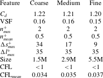

Figure 12. Grid independence study. Comparison of normalized mean velocity components  $U$ and $V$ and Reynolds stress $\langle u^{\prime }v^{\prime }\rangle$. (a) Three locations are selected for the comparison at $z=0~\text{m}$. (b) Coarse (
 ), medium ( $\boldsymbol{-}\!\!\!\!\boldsymbol{-}\!\!\!\!\boldsymbol{-}$, light blue) and fine (
 ) meshes.
3.3.2 Comparison between 2-D and 3-D cases: unactuated and actuated flows
Proper orthogonal decomposition and fast Fourier transform (FFT) analysis are used to compare the similarities and differences between the 2-D and 3-D flow simulations. First, the differences in the unactuated flow are described, and later the similarities between 2-D and 3-D cases of the actuated flow will be taken into consideration.
Figure 13 shows the first (most energetic) POD mode obtained in the 2-D and 3-D unactuated flow simulations. The vortex shedding is clearly represented in both cases by the same structure topology (figure 13a), but the dominant frequency changes between the two cases. Figure 13(b) visualizes the temporal coefficient FFT and its temporal evolution (orbit plot) of the first POD mode. The shedding motion peak is distinct in both cases, being  $F^{+}=0.21$ for the 2-D case and $F^{+}=0.16$ for the 3-D case. For clarity, four phases of the evolution of the 3-D shedding structures are presented in figure 13(c). The source of this discrepancy can be found in the inherited three-dimensionality of the 3-D case. In fact, the presence of a lower energy mode, travelling along the $z$ direction, is observed during the POD analysis.

Figure 13. The shedding mode of the unactuated 2-D (left) and 3-D (right) cases, represented by POD. (a) Structure topology. (b) Analysis of the temporal POD coefficient. The power spectral density (PSD) and the orbit plot of the shedding mode are represented. (c) Four phases of the evolution of the Fourier mode taken at the 3-D shedding frequency  $F^{+}=0.16$.
Figure 14(a) shows the FFT of the temporal coefficient and the structure representation of this transverse mode. From this figure, one can notice that the mode dominant frequency is very close to the 3-D shedding frequency, possibly driving the shedding towards a slower motion when compared to the 2-D case. Since the POD temporal coefficient of this mode shows extra non-dominant peaks, it would be clearer to extract the Fourier mode at  $F^{+}=0.16$ and produce its relative 3-D isosurface plots. The pattern shown by figure 14(b) is clear: a 3-D and a front view perspective show the four phases that describe the evolution of this mode. Yellow and blue structures alternate recursively along the $z$ direction, showing an opposite direction of motion from one side to the other. While on the right side (positive $y$) the yellow structures move upwards (from phase 1 to phase 4), on the opposite side (negative $y$) the yellow structures move downwards (from phase 1 to phase 4), creating a wavy pattern impossible to simulate in 2-D cases.

Figure 14. The transverse mode found in the 3-D unactuated case represented by POD. (a) PSD of the POD temporal coefficient and POD structure topology. (b) Four phases of the evolution of the Fourier mode taken at the 3-D transverse mode frequency  $F^{+}=0.165$, 3-D (top) and front (bottom) views.
The first behaviour one can notice in the actuated case is that the vortex shedding frequency is stabilized by the control into a 2-D-like vortex shedding. Figure 15(a,b) shows the first POD mode of the 2-D and 3-D controlled cases. The vortex shedding remains the most energetic mode even when the control is engaged. Moreover, the 2-D and 3-D sheddings now stabilize on the same frequency, being  $F^{+}=0.21$ (the same frequency as observed for the 2-D unactuated case, figure 13b). In both cases the shedding is very regular and recursive. A clear peak is identified by the PSD of the POD temporal coefficient and the orbit plots evolve regularly and predictably with time, figure 15(b). A similar comparison can be done for the dominant control frequency $F_{1}^{+}$ (2.1), figure 15(c,d). Also here, the similarity between 2-D and 3-D is evident considering the structure topology and the POD temporal coefficient dominant frequency. This mode moves symmetrically on the $xy$ plane since an in-phase control signal is given both to the right and left actuators. In addition, the mode appears stronger close to the side recirculation bubble, fading out progressively downstream. It remains more challenging to distinctively find the secondary control frequency $F_{2}^{+}$ (2.1) by using the POD approach. The energy associated with this frequency is very low ( $A_{1}^{+}$ is one order of magnitude larger than $A_{2}^{+}$ in (2.1)). Therefore the mode is indistinguishable utilizing an energy ranking-based approach. Nevertheless, the respective Fourier mode of $F_{2}^{+}$ can be easily extracted and plotted for comparison.

Figure 15. The shedding mode and  $F_{1}^{+}$ mode of the actuated 2-D (left) and 3-D (right) cases, represented by POD. (a) Structure topology of the shedding mode. (b) Analysis of the temporal POD coefficient. The PSD and the orbit plot of the shedding mode are represented. (c) Structure topology of the $F_{1}^{+}$ mode. (d) Analysis of the temporal POD coefficient, the PSD and the orbit plot of the $F_{1}^{+}$ mode are represented.
A similar structure topology is again observed between the 2-D and 3-D case, figure 16. In this figure, the ellipses (– – –, red) and ( $\boldsymbol{-}\,\boldsymbol{\cdot }\,\boldsymbol{-}$, green) are added as reference to ease the visualization of similar structures. In contrast to the previous $F_{1}^{+}$ mode, the $F_{2}^{+}$ mode visualized here presents an antisymmetric nature (with respect to the $y$ axis) and it has a stronger effect downstream in the wake of the model. One possible explanation for describing the difference of modes is based on their energy content. Since the $F_{1}^{+}$ mode is more energetic, it dominates the region near its generation (the actuator slot and the side of the model). On the contrary, the $F_{2}^{+}$ mode is transported downstream by the antisymmetric shedding mode (which might be the reason for its antisymmetric connotation) and excited in the wake, where it shows its highest energy content.
To reinforce this supposition, the spatial distribution of the energy level of the shedding frequency, and the primary ( $F_{1}^{+}$) and secondary ( $F_{2}^{+}$) control frequencies are presented in figure 17. In particular, figure 17(a) shows the 2-D distribution and 17(b) shows the 3-D distribution, averaged over the homogeneous direction $z$, and presented in a 2-D plot for clarity. The shedding frequency and $F_{1}^{+}$ have the same colour scale, while a dedicated colour scale is given to $F_{2}^{+}$ to account for the lower energy content in this frequency. In addition, to better individuate the region with the highest energy level, (– – –, yellow) describes the contour lines at half of the maximum energy level, for each frequency. The $F_{1}^{+}$ mode has a comparable energy level to the shedding mode, but the area of interest of the primary frequency is confined very close to the actuation and in the side recirculation bubble. On the contrary, the area of interest of the shedding frequency extends longer in the wake of the model, introducing a higher global energy level. Of particular interest is the distribution of the secondary frequency. In both 2-D and 3-D this distribution extends further down in the wake, having its energy peak in the shear layers of the wake. As mentioned before, this low energy frequency seems to be transported downstream by the shedding motion acting in an antisymmetric fashion and predominantly in the wake. Moreover, by looking at the global comparison of these frequency distributions between the 2-D and 3-D cases, a good agreement is observed, corroborating the two-dimensionalization speculation mentioned at the beginning of this section. In other words, the control stabilizes the flow towards a 2-D behaviour, justifying the 2-D optimization process. Therefore, in the next section, we will discuss the 3-D controlled case and the benefit that a multi-frequency (based on vortex shedding harmonics) actuation brings compared to single-frequency (based on higher frequencies) controls. Three 3-D cases will be analysed: the unactuated, the multi-frequency control found by the 2-D GA optimization and a single-frequency control suggested from previous literature (high frequency to suppress the side recirculation).

Figure 16. Fourier mode distribution of the  $F_{2}^{+}$ mode. The 2-D (a) and 3-D (b) actuated cases are presented. Ellipses (– – –, red) and (— —, green) are added as reference to ease the visualization of similar structures.

Figure 17. The distribution of the energy of one single frequency over the sampled domain: (a) 2-D case; and (b) 3-D case. From left to right: shedding frequency,  $F_{1}^{+}$ and $F_{2}^{+}$. For an easier comparison, the distributions are averaged over the homogeneity direction $z$. Dashed line (– – –, yellow) represents the contour lines at half of the maximum energy of each frequency over the sampled domain.
3.4 Superiority of a GA-driven optimization versus previously published achievements
In this last section we want to compare the present GA-driven approach to previously published results, and highlight the advantages of a global drag reduction (GDR) approach to flow control. The use of flow control for this type of bluff body can in fact be driven by a local or a global approach. The first one aims to reduce, or eventually suppress, specific recirculation regions, keeping the flow locally attached to the body surface. The second takes into consideration only global quantities, e.g. the effect of the control on drag reduction. A confined phenomenon, like the appearances of localized flow separations, is usually defined by a limited number of variables. Referring to the side recirculation bubble visualized in figure 3(a), previous research (Minelli et al. Reference Minelli, Krajnović, Basara and Noack2016, Reference Minelli, Adi Hartono, Chernoray, Hjelm, Krajnović and Basara2017b) has shown that a careful selection of the actuator position and frequency can lead to the complete suppression of this local phenomenon. Nevertheless, this does not necessarily optimize global quantities like the total drag. When multiple variables come into play, the use of a global optimization approach is therefore preferable. In particular, it is shown here that sacrificing the suppression of the side recirculation does lead to a lower drag and improved lateral stability. Therefore, two control cases are compared: the side-recirculation-suppression (SRS) case and the GDR case. The former uses a specific frequency indicated by previous literature (Minelli et al. Reference Minelli, Krajnović, Basara and Noack2016, Reference Minelli, Krajnović and Basara2018) to suppress the side bubble, while the latter case is introduced in § 3.2 and obtained from the GA optimization procedure.
Figure 18 shows the comparison of the averaged streamwise velocity and flow topology of the three considered cases, while table 4 lists the averaged drag and side force coefficients together with their respective root mean square (r.m.s.) values. The actuation placed at the front rounded corners significantly affects both the topology of the side and the wake regions. Using a single-frequency actuation signal, with  $F^{+}=fD/U_{\infty }=3$, the side recirculation bubble is completely suppressed (SRS case), while the GDR case, controlled by a two-frequency signal, shows the persistence of this feature. The side recirculation region is therefore not directly connected to a lower drag value.
From this comparison, it does in fact seem rather beneficial to keep a separated flow at the side region in order to obtain a lower drag. The presence of this bubble surely influences the wake topology. Moreover, the presence of the side recirculation could be one of the factors improving the propagation of the actuation frequencies into the wake. The shear layer detaching at the leading edge (after the actuation slot) contains and may transport structures characterized by the actuation frequencies to the trailing edge. In SRS, on the other hand, the shear layer reattaches very early after the actuation slot, exhausting the energy of the actuation frequency on the wall of the model. Considering the two actuated cases and as previously found for a square-back D-shaped body (Barros et al. Reference Barros, Borée, Noack, Spohn and Ruiz2016; Dalla Longa et al. Reference Dalla Longa, Morgans and Dahan2017), a longer wake (in this case GDR) is associated with a lower drag. However, this is not the only factor that describes the drag–wake relationship. The combination of the wake length with its reverse velocity, width and its dynamics complete its description. In addition, the unactuated case presents a substantially different wake topology, in which the side separation merges with the wake and the flow does not reattach at the trailing edge as experienced by the controlled cases (and by the 2-D unactuated case). This is probably the reason behind the longer wake produced by the 3-D unactuated case.

Figure 18. A comparison of the wake topology in 3-D cases with and without actuation. The unactuated and actuated flow-averaged streamwise velocity is shown. The bottom right picture highlights the comparison of the averaged flow topology: (– – –, red) unactuated case; (—  $\boldsymbol{\cdot }$ —, green) GDR case; ( $\cdots \cdots$, yellow) SRS case.
By looking at the minimum reverse velocity extracted from every snapshot and visualized in figure 19, one can obtain a first indication of the wake core movement and its intensity. For clarity, the wake core is taken as the position with the highest reverse velocity value; therefore, each dot in figure 19 represents the location of the wake core and they are coloured by its intensity. In the unactuated case, the reverse velocity is high and the position of the wake core varies in both the  $y$ and $x$ directions. The GDR case, figure 19(b), shows a much lower (absolute) value of the reverse velocity and a narrower area of interest of the wake core position. The SRS case (figure 19c) instead presents a much more confined region of the wake core, which mostly varies its location along $y$. This case also presents a higher reverse velocity compared to the GDR case. This last parameter seems to better relate to the drag value, having the highest reverse velocity for the unactuated case, and the lowest for the GDR case, which gives the lowest drag value.
Table 4. Values of  $C_{d}$, $C_{s}$, their r.m.s. values and the shedding frequency $F_{s}^{+}$ of the unactuated, GDR and SRS cases.
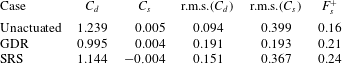

Figure 19. A scatterplot of the highest reverse velocity in the wake: (a) unactuated case; (b) GDR case; and (c) SRS case. Each dot represents the position of the highest reverse velocity for one single snapshot, spatially averaged along the homogeneous direction  $z$; 1000 snapshots are analysed for each case.
Up to this point, the GDR flow control case is shown to contribute to a 20 % drag reduction, while the SRS case improves drag only by 8 %; see table 4. In terms of drag reduction, the GDR case is shown to be significantly more effective than the previously published control strategies; therefore it is also important to verify the lateral fluctuations induced by the two controls. Considering table 4 and figures 20–22, one can better understand the dynamics of the wake and its implications in terms of stability. The natural vortex shedding observed in the unactuated case has a strong influence on  $C_{s}$, resulting in a high r.m.s.( $C_{s}$) value. The same high value is recorded for the SRS case, while the GDR case shows a much lower fluctuation of $C_{s}$. This is also clarified by figure 20, which depicts the $C_{s}$ time history of the three cases. Having a low r.m.s.( $C_{s}$) increases the lateral stability, avoiding unwanted forces created by the shedding motion.

Figure 20. The  $C_{s}$ time history of the three cases: (a) unactuated case; (b) GDR case; and (c) SRS case.
For a deeper analysis of the wake motion, one can concentrate on figures 21 and 22. With the same approach as described in § 3.2, a proximity map and a clustering procedure on the 3-D flow field is presented here. The scatterplots are coloured by  $C_{d}$, $C_{s}$ and the respective cluster number (from left to right in figures 21 and 22). Considering the GDR case (figure 21), one can clearly recognize the recursive side force variation and the periodic alternation of low- and high-drag states. Figure 21 shows in fact that clusters 2 and 4 are defined by high drag values, while 1 and 3 are characterized by low drag. In addition, clusters 2 and 4 show the highest side force values (of opposite sign). By a 3-D representation of velocity isosurfaces, one can better visualize the feature of each cluster. Figure 21(b,c) shows a 3-D and a top view of these isosurfaces, highlighting in yellow the wake core (the region containing the highest reverse velocity value). Clusters 1 and 3 (low drag) show a more elongated and distant-from-base wake cores, while clusters 2 and 4 (high drag) show a more contained and very close-to-base wake cores. Clusters 2 and 4 then not only individuate the oscillation of the side force component, but they are also associated with the highest drag force. This phenomenon is an indication of the presence of a breathing mode of the wake core, whose motion is strongly related to the drag oscillation. In other words, figure 21 shows the periodic elongation and translation of the wake core (yellow isosurface in figure 21b,c) from high- to low-drag states. In particular, looking at the same figure, the representation of clusters 2 and 4 shows a more circular vortex core, with its centre positioned between $x=1$ and $x=1.5$, while in clusters 1 and 3 the core centre is located at $x=2$ and presents a more elongated shape. The alternation of these two states gives rise to the breathing mode introduced earlier and characterizes the periodic motion in the $x$ direction of the wake.
Keeping figure 21 in mind, one can compare it with figure 22. In contrast to the GDR case, figure 22(a) does not show a clear distinction of low- and high-drag clusters, but it only shows a clear side force distinction between different clusters. This case is described by a lower r.m.s.( $C_{d}$) value, which indicates damped $C_{d}$ oscillations, due to the reduction of the streamwise motion of the wake core. The latter, represented in figures 19(c) and 22(b,c), remains in fact close to the model base surface, and it only oscillates in the $y$ direction, strongly affecting the side force rather than the drag and its breathing mode. From these results, one can infer that the propagation of the control frequency downstream in the wake has a beneficial effect on the stability control of the wake motion.

Figure 21. The GDR case, 3-D LES. (a) Proximity maps: left coloured by  $C_{d}$ values, centre coloured by $C_{s}$ values, and right coloured by clusters. (b) Each phase is the average of the snapshots falling in each cluster. The probability of each cluster is equally distributed.

Figure 22. The SRS case, 3-D LES. (a) Proximity maps: left coloured by  $C_{d}$ values, centre coloured by $C_{s}$ values, and right coloured by clusters. (b) Each phase is the average of the snapshots falling in each cluster. The probability of each cluster is equally distributed.
This is corroborated by figure 23, which shows the propagation of the shedding and actuation frequency for the SRS case. The same figure also shows the control frequency Fourier mode visualized with 3-D structures. Comparing this visualization to figure 17(b) (GDR case), it is clear to observe a stronger penetration of the control frequency into the wake in favour of the GDR case. In the SRS case in fact, the actuation frequency remains very localized to the side of the model and no observable energy content is shown in the wake in comparison to the energy content of the shedding frequency. Therefore, an actuation that may effectively control the wake dynamics is preferable compared to a localized control, if the overall drag reduction represents the main deliverable of an optimization study.

Figure 23. The distribution of the energy of one single frequency over the sampled domain, SRS case. From left to right: shedding frequency,  $F_{1}^{+}$ and a 3-D representation of $F_{1}^{+}$ (Fourier mode). (– – –, yellow) represents the contour line at half of the maximum energy of each frequency over the sampled domain.
4 Conclusions and future development
The use of aerodynamic flow control for a square cylinder with lightly rounded leading edges is investigated. The flow control actuators are positioned at the front rounded corners with the intention to reduce drag by the control of the side recirculation bubble and the wake dynamics. A genetic algorithm (GA) optimization on a 2-D grid is conducted to obtain an effective actuation signal for drag reduction. Some 3-D large-eddy simulations (LES) at  $Re=40\,000$ of the unactuated and two selected actuated cases are conducted after the GA process. First, similarities and differences between 2-D and 3-D simulations have been assessed to verify the GA optimization worthy of use. Despite some differences in the vortex shedding frequency of the unactuated flow (presumably induced by spanwise 3-D effects), the controlled case is found to be very similar on comparing 2-D and 3-D simulations. The control is therefore presumed to play an important role in the two-dimensionalization of the 3-D flow field. In 3-D, a significant drag reduction of 20 % is observed using the signal generated by the 2-D GA procedure.
An analysis of the flow in terms of mean and instantaneous quantities is reported. One important aspect discussed is the ability of the actuation to penetrate downstream in the wake, hence affecting its dynamics. By the analysis of the instantaneous flow (using fast Fourier transform (FFT), proper orthogonal decomposition (POD) and clustering), the actuation is shown to influence the wake effectively, reducing drag and lateral instabilities. The GA-optimized actuation or global-drag-reduction (GDR) case has also been compared with a side-recirculation-suppression (SRS) actuation case. The former was shown to be superior in terms of drag reduction and improved stability due to the capacity of the control to propagate into the wake. The SRS case, despite the complete suppression of the side recirculation bubble, shows only 8 % drag reduction and a persistent lateral instability induced by a strong vortex shedding. The dynamics of the vortex shedding and the wakes of the two cases have also been analysed and compared. In the GDR case, a breathing mode of the wake core in the streamwise direction is observed and associated with drag fluctuations. The wake core shows a lower reverse velocity, and a 33 % longer wake compared to the SRS case is observed.
To conclude, two main things are shown in this work. The first one is that a GA procedure suggested an interesting control strategy based on vortex shedding superharmonics, whose frequencies were very effective to improve the overall aerodynamic performance. The second is that an upstream control is shown to be capable of wake dynamics control, possibly substituting an expensive direct-wake control using a lower-energy upstream control.
The authors have in mind two main points as a natural continuation of this work: (i) A more detailed investigation of the propagation property of different actuation frequencies. In this line, it is of major importance to investigate in depth the relation between the actuation wavelength, the length of the body and the dimension of the wake. (ii) Although the study shows promising indications regarding the use of a low-energy control, considerations on energy consumption need to be carefully addressed. Hence, a comparison between classic direct-wake control and the present upstream control will be considered, showing benefits and limits of an upstream control case.
Acknowledgement
The computations were performed on resources provided by the Swedish National Infrastructure for Computing (SNIC) at LiU.
Declaration of interests
The authors report no conflict of interest.


 Open access