


1. Introduction
We study the flow around a wall-mounted circular cylinder, which is of relevance for various technical applications and problem classes in hydraulic engineering, turbomachinery and aeronautics. This flow has a lot in common with flows around more generally shaped bluff bodies mounted on a flat plate. When a turbulent boundary layer approaches such a bluff body, a characteristic vortex system develops at the body–wall junction. This vortex bends around the obstacle and is, therefore, called a horseshoe vortex (Melville & Raudkivi Reference Melville and Raudkivi1977; Baker Reference Baker1980). The horseshoe vortex is commonly assumed to govern the dynamics of body–wall junction flows and has been demonstrated to drive the local scour development, e.g. around bridge piers (see for example Dargahi Reference Dargahi1990). As many bridge failures were caused by scoured foundations (Imhof Reference Imhof2004), a large number of investigations were devoted to exploring the dynamics of the horseshoe vortex system in the context of scouring (for example by Das, Das & Mazumdar Reference Das, Das and Mazumdar2013).
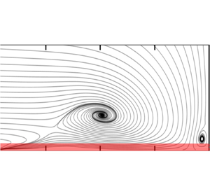
The shear in the boundary layer approaching a wall-mounted bluff body generates a vertical pressure gradient at its front. This pressure gradient, in turn, causes a downflow transporting fluid of high momentum towards the bottom wall where it is deflected mainly in the upstream direction, and forms the horseshoe vortex as well as an upstream-directed wall-parallel jet (Devenport & Simpson Reference Devenport and Simpson1990). This jet develops from the position where the downflow impinges at the bottom wall, passes under the horseshoe vortex and penetrates under the oncoming flow, see figure 1.

Figure 1. Sketch of the horseshoe vortex system.
The horseshoe vortex is characterized by a complicated dynamics (see e.g. Devenport & Simpson Reference Devenport and Simpson1990 or Apsilidis et al. Reference Apsilidis, Diplas, Dancey and Bouratsis2015). These dynamics causes strongly enhanced levels of turbulent kinetic energy (TKE) around the horseshoe vortex core and bi-modal velocity distributions between the vortex core and the wall. Between the cylinder and the horseshoe vortex, where the wall shear stress attains its maximum values, the TKE itself is relatively small (Schanderl et al. Reference Schanderl, Jenssen, Strobl and Manhart2017b). There is a thin layer in which the production of TKE is negative due to the normal stress production term  $- \langle u' u' \rangle \partial \langle u\rangle/\partial x, \langle (.) \rangle$ being the average and $(.)'$ being the fluctuation. Furthermore, turbulent stresses play a minor role in the momentum transport towards the wall (Schanderl, Jenssen & Manhart Reference Schanderl, Jenssen and Manhart2017a). According to these findings, it appears unlikely that the wall shear stress can be assessed accurately by measuring turbulent stresses or by applying a wall model relying on the logarithmic law of the wall. Numerical studies solved this problem by employing a high spatial resolution in the wall-normal direction around the cylinder (Kirkil, Constantinescu & Ettema Reference Kirkil, Constantinescu and Ettema2009; Escauriaza & Sotiropoulos Reference Escauriaza and Sotiropoulos2011; Schanderl & Manhart Reference Schanderl and Manhart2016).
The high wall-normal resolution applied in the mentioned numerical studies leads to a ‘wall-resolved’ simulation in which the wall shear stress can be computed from the first grid points off the wall which have to lie within the viscous layer. In contrast, a wall-modelled simulation applies a coarser grid spacing and estimates the wall shear stress by assuming a certain functional dependence, such as the law of the wall. Both simulation strategies – wall resolved and wall modelled – suffer from problems and open questions. Wall-resolved simulations experience a severe challenge for large Reynolds numbers due to ever finer grids near the wall. Furthermore, it is still unclear how the requirements for the wall-normal resolution scale with Reynolds number. According to the classical estimation by Chapman (Reference Chapman1979),  $O(Re^{1.8})$ degrees of freedom have to be resolved for the representation of the dynamics of the inner layer. However, this estimate is based on the assumption of the classical turbulent boundary layer scaling. Schanderl et al. (Reference Schanderl, Jenssen and Manhart2017a) demonstrated that the stress balance in the wall layer does not follow the classical near-wall scaling, which has two consequences. First Chapman's estimation does not apply here. Second, the wall-modelled simulations based on the logarithmic law of the wall will not perform well in this situation.
The failure of the logarithmic law of the wall can be taken as an explanation for the difficulties in determining experimentally the wall shear stress from velocity measurements in front of a cylinder–wall junction. Graf & Istiarto (Reference Graf and Istiarto2002) showed that the wall shear stress estimations based on velocities and Reynolds stresses differ strongly there. In this light, Manes & Brocchini (Reference Manes and Brocchini2015) have chosen a different approach using the phenomenological theory of turbulence. For negligible viscous stresses, they argue that the friction coefficient in an equilibrium scour hole scales with the cubic root of the ratio of the grain diameter to the characteristic length scale of the largest eddies. This argument is certainly reasonable for rough surfaces in the high Reynolds number limit in which the friction coefficient depends on the relative roughness only. However, many experiments and simulations have been performed at lower Reynolds numbers and over smooth walls. The understanding, quantification and simulation of the scour process in natural and laboratory scenarios is therefore limited by the little available information on the Reynolds number dependence of the wall shear stress. In view of the failure of the logarithmic law of the wall in large parts of the wall jet under the horseshoe vortex, it seems important to us to study the near-wall behaviour of the velocity profiles with emphasis on their Reynolds number dependence.
Published results indicate that different topologies of the horseshoe vortex system occur dependent on the Reynolds number. At low Reynolds numbers, two or more horseshoe vortices (train of vortices) have been observed (Dargahi Reference Dargahi1989; Doligalski, Smith & Walker Reference Doligalski, Smith and Walker1994; Launay et al. Reference Launay, Mignot, Riviere and Perkins2017). With increasing Reynolds number, this vortex configuration becomes unsteady and can show a chaotic dynamics (Launay et al. Reference Launay, Mignot, Riviere and Perkins2017). At high Reynolds numbers, the time-averaged horseshoe vortex system consists of a single dominant vortex (Devenport & Simpson Reference Devenport and Simpson1990; Apsilidis et al. Reference Apsilidis, Diplas, Dancey and Bouratsis2015; Schanderl et al. Reference Schanderl, Jenssen, Strobl and Manhart2017b). The appearance of the individual regimes seems to be dependent on the Reynolds number based on cylinder diameter, the boundary layer-to-diameter and water depth-to-diameter ratios (Launay et al. Reference Launay, Mignot, Riviere and Perkins2017) and the turbulence in the approaching flow (Kirkil & Constantinescu Reference Kirkil and Constantinescu2015).
The Reynolds number dependence of the turbulence structure around the horseshoe vortex shows no common trend. The simulations of Escauriaza & Sotiropoulos (Reference Escauriaza and Sotiropoulos2011) reveal strong changes between  $Re=2\cdot 10^4$ and $Re=3.9\cdot 10^4$. In the simulations at $Re=1.6\cdot 10^4$ and $Re=5\cdot 10^5$ by Kirkil & Constantinescu (Reference Kirkil and Constantinescu2015) the normalized turbulence level around the horseshoe vortex decreases strongly with Reynolds number. They explain this with the fact that the horseshoe vortex moves closer to the wall with increasing Reynolds number in their simulations. They also conjecture that a realistic representation of the turbulence in the approaching flow suppresses secondary vortices around the horseshoe vortex. In an experimental study Apsilidis et al. (Reference Apsilidis, Diplas, Dancey and Bouratsis2015) measured flow fields in the symmetry plane in front of a cylinder at three different Reynolds numbers ( $Re=2.9\cdot 10^4$, $4.7\cdot 10^4$ and $1.23\cdot 10^5$). The measured flow topology is in line with published results except that they did not resolve the corner vortex directly at the cylinder–wall junction. They did not observe a clear Reynolds number dependence of the position of the horseshoe vortex. However, they observed a clear dependence of the distribution of the TKE on the Reynolds number. At the larger Reynolds numbers, the intensity of a second peak of the TKE (beside the one around the vortex core) under the horseshoe vortex increases, which was also reported by Kirkil & Constantinescu (Reference Kirkil and Constantinescu2015). This peak is caused by the near-wall jet pointing in the upstream direction under the horseshoe vortex (Apsilidis et al. Reference Apsilidis, Diplas, Dancey and Bouratsis2015; Kirkil & Constantinescu Reference Kirkil and Constantinescu2015; Schanderl et al. Reference Schanderl, Jenssen, Strobl and Manhart2017b).
Despite the large amount of literature on the Reynolds number dependence of the topology of the horseshoe vortex system, its dynamics and turbulence structure, knowledge of the behaviour in the immediate wall layer is limited. The open questions include the following. How is the time-averaged wall shear stress linked to Reynolds shear stresses above the wall? How does the time-averaged wall shear stress scale with Reynolds number? Which resolution do we need to accurately estimate the wall shear stress and how does it scale with Reynolds number? What is the thickness of the viscous layer and how does it scale with Reynolds number? Is a classical wall model suited to estimate the wall shear stress from velocities at a larger wall distance? Can we find universal behaviour in the viscous layer or even self-similar velocity profiles? How can we construct a better wall model for the flow in front of the cylinder?
To answer these questions, we investigate the Reynolds number dependence of the near-wall flow by conducting both large-eddy simulation (LES) and particle-image velocimetry (PIV) experiments in front of a wall-mounted cylinder placed in an open channel. We used three moderate Reynolds numbers to study the Reynolds number scaling of the wall shear stress and the near-wall velocity profiles. Our working hypothesis is that the flow can be split into an outer and an inner flow. From the classical description of turbulent boundary layers, the outer flow depends only weakly on the Reynolds number, whereas this dependence is strong for the inner flow due to the dominance of the viscous terms. Based on the results of Apsilidis et al. (Reference Apsilidis, Diplas, Dancey and Bouratsis2015) and the observation that the viscous terms play a negligible role around the horseshoe vortex (Schanderl et al. Reference Schanderl, Jenssen and Manhart2017a), we can expect that the horseshoe vortex belongs to the outer flow, which is only mildly dependent on the Reynolds number in the range considered in this investigation. The validity of this assumption will be assessed in this paper as it is the basis for a clear inner layer scaling.
The paper is organized as follows, first, § 2 presents the flow configuration, while the experimental and the numerical set-ups are documented in §§ 3 and 4, respectively. The outer flow (vortex system, downflow) in front of the wall-mounted cylinder are briefly discussed in § 5. Finally in § 6, the resulting near-wall flow and the wall shear stress are documented before a detailed analysis concerning the applicability of the Falkner–Skan theory is presented.
2. Flow configuration
We investigated the flow around a circular cylinder mounted vertically on the bottom wall of an open channel (figure 2). The centre of the coordinate system is placed in the cylinder axis at the height of the bottom wall. The streamwise, lateral and vertical directions are denoted by  $(x,y,z)$, respectively. We considered three Reynolds numbers, $Re_D=20\ 000$, $Re_D=39\ 000$ and $Re_D=78\ 000$ based on the diameter of the cylinder $D$ and the velocity averaged over the entire cross-section of the approaching flow (bulk velocity $u_b$). The flow depth was $h=1.5D$ for all three Reynolds numbers. However, the ratio of the width of the channel $w$ to the diameter $D$ had to be adjusted for the highest Reynolds number. The width was $w=11.7D$ at $Re_D=20\ 000$ and $Re_D=39\ 000$ and $w=7.3D$ at $Re_D=78\ 000$. This adjustment resulted from experimental constraints: in the experiment, the absolute width of the flume was fixed but the large Reynolds number required a larger flow depth to keep the Froude number $Fr={u_b}/{\sqrt {g h}}$ low. Since the flow depth-to-diameter ratio was considered to have a larger influence on the flow field around the cylinder than the width-to-diameter ratio (Istiarto Reference Istiarto2001; Oliveto & Hager Reference Oliveto and Hager2002), we kept the first one constant while the latter was changed for the highest Reynolds number case. To assess the influence of the width-to-diameter ratio, we simulated the $Re_D=20\ 000$ flow case for both widths $11.7D$ and $7.3D$ individually and observed only minor differences; they were significantly smaller than the changes with Reynolds number. Therefore, we consider the lower aspect ratio at $Re_D=78\ 000$ to have a negligible effect for the orientation of this study. The inflow condition was a fully developed, turbulent open-channel flow with a Froude number of $Fr<0.32$ in the experiments. In contrast, the Froude number in the simulations was infinitesimal, as the free surface was approximated by a slip boundary condition, which prevented all deformations of the free surface.

Figure 2. Sketch of the flow configuration taken from Schanderl et al. (Reference Schanderl, Jenssen, Strobl and Manhart2017b).
Our flow configuration was identical to the one described in detail by Schanderl & Manhart (Reference Schanderl and Manhart2016, Reference Schanderl and Manhart2017) and Schanderl et al. (Reference Schanderl, Jenssen and Manhart2017a,Reference Schanderl, Jenssen, Strobl and Manhartb, Reference Schanderl, Jenssen, Strobl and Manhart2018). The particular depth-to-diameter ratio at  $Re_D=39\ 000$ was selected to be consistent with previous experiments by Link (Reference Link2006), Pfleger (Reference Pfleger2011a) and Pfleger, Rapp & Manhart (Reference Pfleger, Rapp and Manhart2010, Reference Pfleger, Rapp and Manhart2011). The set-up is close to the configuration investigated by Dargahi (Reference Dargahi1989), Escauriaza & Sotiropoulos (Reference Escauriaza and Sotiropoulos2011) and Apsilidis et al. (Reference Apsilidis, Diplas, Dancey and Bouratsis2015), which differs from ours in the ratio of boundary layer thickness to cylinder diameter. However, they were performed in the same range of Reynolds numbers.
3. Experimental configuration
The PIV experiments were conducted in the laboratory of the Chair of Hydromechanics at the Technical University of Munich. The flow configuration was reproduced in a  $1.17\ \mathrm {m}$ wide and $30\ \mathrm {m}$ long flume (figure 3) with a smooth bed and sidewalls. The flow developed naturally over approximately $20\ \textrm {m}$ approaching a circular cylinder placed vertically in the symmetry plane of the flume. At $Re_D=20\ 000$ and $Re_D=39\ 000$, the diameter of the cylinder was $D=0.10\ \textrm {m}$ and $D=0.16\ \mathrm {m}$ at $Re_D=78\ 000$. Thus, the undisturbed inflow length changed from $200D$ for $Re_D=20\ 000$ and $Re_D=39\ 000$ to $125D$ at $Re_D=78\ 000$.

Figure 3. Sketch of the experimental configuration, taken from Pfleger (Reference Pfleger2011b).
We employed two-dimensional two-component PIV in the symmetry plane in front of the cylinder. Hollow glass spheres of diameter  $d_{{p}}=10\ \mathrm {\mu }\mathrm {m}$ and density $\rho _{{p}}=1100\ \mathrm {kg}\ \mathrm {m}^{-3}$ were added continuously to seed the flow. The corresponding relaxation time of $\tau _{{p}}=d_{{p}}^2\rho _{{p}}/(18\nu \rho )=6.1\cdot 10^{-6}\ \mathrm {s}$ (Raffel et al. Reference Raffel, Willert, Scarano, Kähler, Wereley and Kompenhans2007) was three orders of magnitude smaller than the Kolmogorov time scale obtained by the macro-scale estimation of the dissipation rate of the TKE $\epsilon _{{macro}}=u_{{b}}^3/D$ (Pope Reference Pope2011). Thus, the particles behaved as a passive tracer following the flow reasonably well, where $u_{{b}}$ is the depth-averaged velocity in the symmetry plane of the undisturbed flow, $\rho$ the water density and $\nu =1.05\cdot 10^{-6}\ \mathrm {m}^2\ \mathrm {s}^{-1}$ the kinematic viscosity of the water at a temperature of approximately $18\,^\circ$C.
We used a Nd:YAG laser with a wavelength of  $532\ \mathrm {nm}$ for the illumination. The light sheet had a thickness of $2\ \mathrm {mm}$ in the spanwise direction and entered the flow from the top through a slat of acrylic glass, suppressing surface waves. The image pairs were recorded by a CCD camera with a resolution of $2048\times 2048\ \mathrm {px}$ perpendicularly from the side with a time delay of $700\ \mathrm {\mu }\mathrm {s}$ at $Re_D = 20\ 000$ and $Re_D = 39\ 000$ and $850\ \mathrm {\mu }\mathrm {s}$ for $Re_D = 78\ 000$. The pixel size varied between $36.86\ \mathrm {\mu }\mathrm {m}\ \mathrm {px}^{-1}$ and $36.29\ \mathrm {\mu }\mathrm {m}\ \mathrm {px}^{-1}$. The sampling rate of $7.25\ \mathrm {Hz}$ was too low to resolve the temporal evolution of turbulent structures. Hence, we analysed the flow only at the time-averaged level. The images were evaluated by a standard PIV algorithm with interrogation windows of $16\times 16\ \mathrm {px}$ in size and an overlap of 50 %. In case of the detection of an invalid velocity vector, this individual $16\times 16\ \mathrm {px}$ interrogation window was replaced by the corresponding $32\times 32\ \mathrm {px}$ interrogation window with the same position of the window centre. The number of image pairs and the data resolution are listed in table 1.
Table 1. Data resolution and recorded image pairs of the conducted PIV. The numbers of valid velocity vectors refer to the numbers which were achieved in wide regions of the flow.

The standard PIV evaluation was complemented by a single-pixel method (Westerweel, Geelhoed & Lindken Reference Westerweel, Geelhoed and Lindken2004; Kähler, Scholz & Ortmanns Reference Kähler, Scholz and Ortmanns2006; Strobl Reference Strobl2017). This single-pixel PIV (SPPIV) is not based on interrogation windows but provides an ensemble-averaged velocity vector at every individual pixel, which tremendously increases the spatial resolution. The larger data resolution allowed an evaluation of the wall shear stress by resolving the velocity gradient at the wall. The drawback of the SPPIV approach is a larger statistical scatter in the data.
The error in a SPPIV consists of the statistical error (dependent on the number of samples), the numerical error while determining the moments of the correlation functions and the uncertainty in the pixel size and wall position. In a SPPIV, the number of samples is obtained by the number of image pairs multiplied by the average number of particles per pixel (p.p.p.) which was  $N_{ppp}\approx 0.007$ p.p.p. in our measurements. We increased the number of samples by using the symmetric double correlation technique (Avallone et al. Reference Avallone, Discetti, Astarita and Cardone2015) and by averaging the correlation functions over five pixels in streamwise direction, which resulted in an average number of $1950$ samples per data point. This compiles in a statistical root-mean-square deviation in the computed average velocity of approximately $2\,\%$ of its standard deviation. One has to take into account as well the errors from the integration of the moments from the correlation function. These errors are strongly dominated by the noise at the edges of the evaluation window (Strobl Reference Strobl2017) which decays with the square root of the number of images taken. However, its influence on the computed moments of the velocity probability density function (PDF) depends on the size and placement of the PDF in the evaluation window. Therefore, this error can hardly be evaluated a priori. We will give a visual impression of this error in § 6.1.
4. Computational configuration
The numerical datasets were collected by conducting LESs at the three Reynolds numbers  $20\ 000$, $39\ 000$ and $78\ 000$. In the following, the numerical methods are described (section 4.1) and the adjustments of the grids to account for the individual Reynolds numbers are discussed. The influence of the subgrid-scale stress model on the solution is documented in § 4.2. A further validation of the numerical results is presented in § 6.1 by demonstrating that the wall shear stress converges when the grid was refined.
4.1. Numerical method and computational grids
Our in-house code MGLET employs a finite volume discretization on Cartesian grids with a staggered arrangement of variables. Central differences were used for the spatial approximation, a third-order Runge–Kutta scheme for the time integration and zonally embedded grids for local grid refinement (Manhart Reference Manhart2004). The curved surface of the cylinder was represented by a mass-conserving second-order ghost-cell immersed boundary method (Peller et al. Reference Peller, Duc, Tremblay and Manhart2006; Peller Reference Peller2010). The subgrid-scale stresses were modelled using the wall-adapting local eddy viscosity (WALE) model (Nicoud & Ducros Reference Nicoud and Ducros1999). In this approach, the eddy viscosity decreases towards the wall and the Reynolds stresses show correct asymptotic behaviour. Hence, no damping function had to be applied, which facilitates the use of an immersed boundary method.
The fully developed, turbulent open-channel flow was simulated on a precursor grid with periodic boundary conditions in the streamwise direction. A one-way coupling to this grid supplied the inflow condition for the grid containing the cylinder. We have chosen this approach as it is practically impossible to supply instantaneous velocity data at the inflow plane by measurements. We used great care to obtain a satisfying accordance between the simulated and the measured inflow in a statistical sense, see § 5.1. The free surface of the open channel was modelled by a slip boundary condition; thus preventing surface deformations. This corresponds to the limit  $Fr \to 0$. The sidewalls and the bottom wall of the channel were represented by a no-slip boundary condition. The $Re_D=39\ 000$ case was used to design the grid. To achieve the required grid resolution, we successively refined the region around the cylinder until no substantial changes could be observed in the results, especially in the wall shear stress. This state was reached with three locally embedded grids (figure 4), which corresponded to a total refinement factor of eight compared to the global grid. In addition, the base grid was geometrically stretched in the wall-normal direction by less than $1\,\%$, which results in a stretching factor smaller than $0.1\,\%$ of the finest grid level. We applied constant time steps which resulted in Courant–Friedrichs–Lewy numbers below $0.8$ on the finest grids. The minimum simulated time to obtain representative estimates for the first and second statistical moments was $570D/u_{{b}}$ (table 2).

Figure 4. Side view of the computational domain. The embedded grids are highlighted in grey. The embedded grid 1 extends over the entire width of the channel while grids 2 and 3 cover a quadratic area of the  $x$–
$x$– $y$-plane.
Table 2. Grid resolution in the region of interest around the cylinder and sampling time. The wall shear stress applied for the evaluation of the wall units was taken from the corresponding approaching flow.

The reliability of the  $Re_D=39\ 000$ simulation was assessed by Schanderl & Manhart (Reference Schanderl and Manhart2016), the near-wall stress balance is documented by Schanderl et al. (Reference Schanderl, Jenssen and Manhart2017a) and the turbulence structure of the horseshoe vortex is presented by Schanderl et al. (Reference Schanderl, Jenssen, Strobl and Manhart2017b, Reference Schanderl, Jenssen, Strobl and Manhart2018). We scaled the grids for $Re_D=20\ 000$ and $Re_D=78\ 000$ to maintain the spatial resolution in inner units (based on the wall shear stress of the approaching flow) and we observed the same convergence behaviour. The grid spacings of the finest local grids at each individual Reynolds number are listed in table 2.
4.2. Influence of the subgrid-scale stress model
Figure 5(a) illustrates the ratio of the time-averaged modelled (subgrid-scale) viscosity to the molecular viscosity  $\langle \nu _{{t}} \rangle /\nu$ as a function of the $z$ direction (wall normal) in front of the cylinder for $Re_D=78\ 000$. Here, $\langle \cdot \rangle$ stands for the time-averaging operator. The streamwise position $x/D=-0.76$ corresponds to the centre of the horseshoe vortex V1; $\langle \nu _{{t}} \rangle$ was evaluated for three different simulations: LES78k $\#1$, $\#2$ and $\#3$ used one, two and three zonal grid refinements, respectively. The finest grid spacing was four times smaller than the one of LES78k $\#1$. The inner normalization is indicated by $(\cdot )^+$. To facilitate the mutual comparison, the wall units used for normalizing the wall distance are based on the wall shear stress from the simulation with the finest grid for all three profiles.

Figure 5. Time-averaged turbulent viscosity  $\langle \nu _{{t}} \rangle$ taken from three different LESs with different grid resolution (a) and contributors to the stress balance $\nu \langle \partial u /\partial z \rangle$, $\langle \nu _{{t}} \partial u /\partial z \rangle$ and $-\rho \langle u'w'\rangle$ taken from the simulation with the finest grid LES78k $\#3$ (b) in the $z$ direction (wall normal) at $x/D =-0.76$ corresponding to the horseshoe vortex centre at $Re_D=78\ 000$. The wall shear stress was taken from the simulation with the finest grid LES78k $\#3$ to evaluate $z^+$.
For all three simulations, the subgrid-scale viscosity peaks at the position of the horseshoe vortex centre ( $z^+\approx 180$) and decreases towards the wall (figure 5a). The amplitude decreases nearly with second order as the grid spacing is reduced. This can be seen from the peak amplitudes of $\langle \nu _t\rangle /\nu$ in figure 5(a) which are ${\langle \nu _t\rangle /\nu }_{peak}=2.2$, $0.68$ and $0.2$ for LES78k $\#1$, $\#2$ and $\#3$, respectively.
The influence of the modelled viscosity on the stress balance is documented for the finest grid in figure 5(b) by comparing the viscous  $\nu \langle \partial u /\partial z \rangle$, the Reynolds $-\rho \langle u'w'\rangle$ and the modelled subgrid-scale stresses $\langle \nu _{{t}} \partial u /\partial z \rangle$. The stresses are normalized by the absolute value of the local time-averaged wall shear stress $\langle \tau _{{w}} \rangle$. Here, $u$ denotes the velocity component in the $x$ direction (streamwise) while $w$ is the component in the wall-normal direction, $u'$ and $w'$ represent the corresponding velocity fluctuations and $\rho$ is the fluid density. Note that the normalized stresses sum to $-1$ at the wall since the wall shear stress points in negative $x$ direction. The viscous stresses dominate the flow close to the wall. As the modelled viscosity is rather small in this region, the influence of the subgrid-scale stress model is also small. In contrast to the region of the horseshoe vortex, where $\langle \nu _{{t}} \rangle$ is largest, we observe a perceptible contribution of the subgrid-scale stress model to the viscous stresses. However, outside of the near-wall region the resolved Reynolds stresses are significantly larger than the viscous and the modelled stresses.
For  $Re_D=39\ 000$, Schanderl et al. (Reference Schanderl, Jenssen, Strobl and Manhart2017b) showed that the fraction of the modelled TKE is by two orders of magnitude smaller than the resolved one. Furthermore, the modelled dissipation is less than $30\,\%$ of the total dissipation.
5. The outer flow
In figure 5 it can be seen that the viscous stress  $\nu \langle \partial u/\partial z\rangle$ makes a negligible contribution to the momentum balance in the streamwise direction when compared with the turbulent shear stress $-\rho \langle u'w'\rangle$ in the region around the horseshoe vortex centre (at $z^+\approx 100$). If we define the outer flow as the region in which the viscous stresses play a minor role in the momentum balance, the horseshoe vortex belongs to the outer flow. Changes of the outer flow with Reynolds number are attributed to variations of: (i) the shape of the inflow profile; and (ii) the characteristics of the inner region, e.g. changes of the singular points, the wall shear stress or of the near-wall turbulence structure, as they propagate to the outer flow. In what follows, we document the Reynolds number dependence of the approaching boundary layer, the downflow in front of the cylinder, the pressure gradient, the positions of the singular points, the turbulent kinetic energy and the outer velocity profiles around the horseshoe vortex.
5.1. Approaching flow, downflow and pressure gradient
The horseshoe vortex system depends strongly on the profile shape of the approaching flow, the boundary layer thickness and the turbulence structure (Schanderl & Manhart Reference Schanderl and Manhart2016). We did our best to provide comparable inflow conditions in the simulations and the experiments. In the simulations, the inflow was a fully developed, turbulent open-channel flow with all restrictions imposed by modelling and numerical errors. Whereas, in the experiments, the open-channel flow developed within the limited entry lengths of  $133$ water depths at $Re_D=20\ 000$ and $Re_D=39\ 000$ and $83$ water depths at $Re_D=78\ 000$. The time-averaged centreline flow profiles of the approaching channel flow are documented in figure 6. The inner scaling in figure 6(a) reveals a pronounced wake region in the LES while this is not the case in the experiment. This is also visible in the outer scaling (figure 6b). There are many possible reasons for the observed differences between the LES and PIV profiles of which some are (i) the upper boundary condition, (ii) the relatively coarse LES grid in the precursor simulation, especially at the lateral wall, and (iii) possible effects of the subgrid-scale (SGS) model in the precursor simulation. However, LES and PIV show a clear trend towards profiles displaying a progressively increasing mixing in longitudinal momentum, with increasing Reynolds number.

Figure 6. Time-averaged velocity profiles in the centre of the approaching flow in inner scaling (a) and outer scaling (b). The symbols mark the LES data at every tenth data point.
The downflow in front of the cylinder can be considered as an upper boundary condition for the near-wall flow and the horseshoe vortex. Figure 7(a) shows horizontal profiles of the time-averaged vertical velocity  $\langle w\rangle /u_{{b}}$ at $z/D=0.15$ for all cases. The downflow reveals a sharp peak at $x/D\approx -0.52$. The corresponding values are approximately $-0.4 u_{{b}}$ in the experiment and $-0.5 u_{{b}}$ in the simulation. This is a considerable fraction of the inflow momentum. Upstream of the maximum of the downflow, the profiles decrease over a distance of $0.3D$ and do not change significantly with Reynolds number. Thus, potential Reynolds number effects on the flow are not obscured by inconsistent boundary or inflow conditions. The accordance between LES and PIV is satisfactory; the differences could be assigned to the horizontal slat of acrylic glass at the free surface in the experiment, which was used to enable an undisturbed light sheet entering the water body (section 3). This slat moved the upper stagnation point on the cylinder front a little downwards compared with the LES. Consequently, the momentum of the downflow is smaller in the experiment (figure 7a). We will discuss this effect on the vortex system in § 5.2.

Figure 7. Time-averaged horizontal profiles of the vertical velocity at  $z/D=0.15$ (a), and the pressure coefficient $c_{{p}}$ at the bottom wall in front of the cylinder (b).
The downflow reaching the bottom wall causes the pressure to increase. The location of the maximum value of the horizontal pressure distribution corresponds to the position of the minimum value of the vertical velocity component in the downflow. This is indicated by figure 7(b) showing the pressure coefficients  $c_{{p}}=(p-p_{{ref}})/(\frac {1}{2}\rho u_{{b}}^2)$ from the LES data. The reference values of the pressure $p_{{ref}}$ are chosen that the pressure coefficients are zero at the corner between the cylinder and wall. The distribution has been validated for $Re=39\ 000$ by (Schanderl & Manhart Reference Schanderl and Manhart2016) by comparing to the distribution measured by Dargahi (Reference Dargahi1989). The peak values of the pressure distributions occur at $x/D\approx -0.54$ decreasing steeply in the upstream direction until $x/D \approx -0.7$ with a slight kink at $x/D\approx -0.6$. Upstream of $x/D\approx -0.9$, the pressure gradient is constant but smaller. In both regions, the pressure coefficient is independent of the Reynolds number. In between, the nearly constant steep and mild pressure gradients are separated by a disturbance linked to the horseshoe vortex. The amplitude, the spatial extent and the distance from the cylinder of this disturbance increase with Reynolds number.
5.2. Horseshoe vortex system
The flow configuration at the cylinder–wall junction is illustrated by streamlines of the time-averaged flow field taken from the LES at  $Re_D=39\ 000$ (figure 8). The in-plane downflow impinges at S3 (a half-saddle) and is mainly deflected in the upstream direction; a small part is redirected towards the cylinder. The location of S3 corresponds to the position of the maximum of the pressure at the bottom wall and to the peak of the downflow (figure 7). One part of the downflow is entrained into the horseshoe vortex V1 (a node). The rest forms a jet in the upstream direction along the bottom wall underneath V1, highlighted by the separating streamline. This jet dominates the behaviour of the wall shear stress as the further analysis will show. The wall-parallel jet starts to develop from S3 and penetrates until the half-node N1 (a saddle point in the walls shear stress vector field). Between N1 and S1, a flow reversal occurs on top of the jet, which is separated from V1 by the saddle point S1. The downflow generates a boundary layer along the cylinder front, which separates at S4 (a half-saddle) and forms a small vortex V3 (a node) directly at the cylinder–wall junction. The configuration of the singular points at the cylinder–wall junction is in accordance between LES and PIV and does not change with Reynolds number.

Figure 8. Streamlines of the time-averaged flow field in the symmetry plane in front of the cylinder with singular points for  $Re_D=39\ 000$ computed from LES (top) and PIV (bottom). The black line indicates the separating streamline of the horseshoe vortex and the wall-parallel jet. Note the two different scales of the $x$-axis for which $x_{adj}$ is adjusted between the stagnation point S3 and the horseshoe vortex centre V1. The measurement data only extend to $x/D = -1.06$.
The terms half-node and half-saddle are rational given the topological considerations presented in Foss (Reference Foss2004) and Foss et al. (Reference Foss, Hedden, Barros and Christensen2016). They refer to singular points on a seam of a collapsed sphere. With that understanding, the streamline that stagnates on the cylinder (above the domain shown in figure 8) represents the upper leg of the seam that continues through S4, S3 and past N1. The upstream hole in the collapsed sphere (between the lower surface and the identified stagnation streamline) leads to the a priori Euler characteristic  $\chi _A= +1$. The experimental Euler characteristic observed in figure 8: $\chi _E = 2 \sum N + \sum N' - 2 \sum S - \sum S' = 2(2) + 1 - 2(1) - 2 = + 1$, is in agreement with $\chi _A$, providing assurance that no further singular points are required to satisfy the topological constraint.
We document the positions of the singular points for the three Reynolds numbers in table 3. Both, vortex V1 and saddle point S1 move in the upstream direction away from the cylinder with increasing Reynolds number, which is in line with the observations of Agui & Andreopoulos (Reference Agui and Andreopoulos1992). In contrast, the half-node N1 and the corresponding recirculation zone move towards the cylinder. This can be explained by the larger near-wall momentum of the approaching flow at the higher Reynolds number, which counteracts the penetration of the jet. Therefore, the distance between the upstream point N1 and V1 decreases with increasing Reynolds number in the investigated range.
Table 3. Positions of the singular points obtained by LES and PIV.

In the experiment, the horseshoe vortex V1 has a smaller extent and is located closer to the cylinder. Due to the slat of acrylic glass, the momentum of the downflow is smaller and could cause the observed differences here as well.
There is common agreement that in the considered flow the distribution of the TKE has a distinct c shape (Devenport & Simpson Reference Devenport and Simpson1990; Paik, Escauriaza & Sotiropoulos Reference Paik, Escauriaza and Sotiropoulos2007; Apsilidis et al. Reference Apsilidis, Diplas, Dancey and Bouratsis2015; Schanderl et al. Reference Schanderl, Jenssen, Strobl and Manhart2017b). The upper branch of the c is formed by a peak of TKE in the region of the main vortex V1, from where a leg-like peak reaches towards the bottom wall and thus forms the lower branch of the c. To the upper branch, the fluctuations of the vertical velocity component  $w'$make a strong contribution, while the lower branch results from strong fluctuations in the streamwise direction $u'$ predominantly (Devenport & Simpson Reference Devenport and Simpson1990; Apsilidis et al. Reference Apsilidis, Diplas, Dancey and Bouratsis2015; Schanderl et al. Reference Schanderl, Jenssen, Strobl and Manhart2017b). The lower branch is located where the jet decelerates. As observed by Apsilidis et al. (Reference Apsilidis, Diplas, Dancey and Bouratsis2015), the amplitude of $u'$ in this jet increases with Reynolds number and the lower branch of the c shape becomes more pronounced. All the mentioned features are visible in the distribution of the in-plane TKE $k_{ip}=0.5 (\langle u'u'\rangle +\langle w'w'\rangle )$ presented in figure 9 for both LES and PIV at all three Reynolds numbers. The change with Reynolds number is consistent with the observation of Apsilidis et al. (Reference Apsilidis, Diplas, Dancey and Bouratsis2015) in that the distribution and magnitude of in-plane TKE around the horseshoe vortex centre is only weakly dependent on Reynolds number. In the leg under the horseshoe vortex, an increase in TKE is observed in both experiment and LES. This suggests that the turbulence structure of the horseshoe vortex system is only mildly dependent on Reynolds number in the considered range.

Figure 9. In-plane TKE  $k_{ip}/u_b^2$ in the symmetry plane in front of the cylinder for $Re=20\ 000$ (a,b), $Re=39\ 000$ (c,d) and $Re=78\ 000$ (e,f), taken from the LES (left column) and the PIV (right column).
5.3. Outer velocity profiles
Figure 10 shows the profiles of the streamwise velocity component normalized by the bulk velocity  $\langle u \rangle /u_{{b}}$ at five positions in the symmetry plane in front of the cylinder. The data were taken from the LES. Since the position of vortex V1 changes slightly with Reynolds number, we introduce an adjusted streamwise coordinate $x_{{adj}}$ to compare the profiles at identical positions with respect locations of the horseshoe vortex centre $x_{{\textrm {V}1}}$ and the stagnation point $x_{{\textrm {S}3}}$
 \begin{equation} x_{{adj}}=\frac{x-x_{{\textrm{S}3}}} {x_{{\textrm{S}3}}-x_{{\textrm{V}1}}},\end{equation}
where  $x_{{adj}}=0$ corresponds to $x_{{\textrm {S}3}}$ and $x_{{adj}}=-1$ is the position of the horseshoe vortex V1 (see figure 8 for $Re_D=39\ 000$). In the wall-normal direction, the location of vortex V1 did not change, thus no comparable adjustment was applied to the $z$ coordinate.

Figure 10. Wall-normal profiles of the streamwise velocity component normalized by the bulk velocity  $\langle u \rangle / u_{{b}}$ in the symmetry plane in front of the cylinder at different positions of the adjusted coordinate $x_{{adj}}$ taken from the LES.
The upstream-directed wall jet is indicated by the negative  $\langle u \rangle / u_{{b}}$ close to the wall. This jet is accelerated from stagnation point S3 ( $x_{{adj}}=0$) in the upstream direction by the pressure gradient. The velocity profiles reveal a sharp peak, which increases to its maximum value of approximately $0.5u_{{b}}$ at $x_{{adj}}=-0.75$. This is around the location at which the dividing streamline indicated in figure 8 is closest to the wall.
With further increasing distance from the cylinder, the jet widens vertically due to the influence of the horseshoe vortex. As a result, the jet starts to decelerate and the velocity peak begins to lift off from the bottom wall around the position of the vortex core ( $x_{{adj}}=-1$). This mechanism is indicated by the $c_{{p}}$-distribution and the streamlines (figure 7 and figure 8). Between $x_{{adj}}=-0.25$ and the position of the vortex centre at $x_{{adj}}=-1$, the peak is consistently largest at $Re=78\ 000$ and smallest at $Re=20\ 000$, but the velocity difference is small. Above the (negative) velocity peak, the normalized profiles seem to be essentially Reynolds number independent, except at positions upstream of the vortex core ( $x_{{adj}}<-1$).
Together with the observation of  $c_{{p}}$ being independent of Reynolds number, this allows us to introduce the conceptional division into an outer and an inner flow in which the outer flow is only marginally dependent on the viscosity, whereas the inner flow is strongly affected by viscous effects. In figure 11(a), the two regions are illustrated with the help of the time-averaged velocity profile at $x/D=-0.6$. The peak velocity of the jet is denoted as $u_\delta$ and the corresponding wall distance as $\delta _{{s}}$. This characteristic point marks the boundary between the inner and the outer flows. For $Re\to \infty$, the layer affected by the wall would become arbitrarily small. Figure 11(b) shows that the viscous stress is large in the inner layer and almost zero in the outer layer; conversely, the turbulent stress is large in the outer layer and reduces quickly to zero in the inner layer. While the viscous stress is negative in the inner layer due to the negative velocity gradient, the turbulent stress is positive. As a result, the production of turbulent kinetic energy changes sign from positive to negative when crossing the boundary from outer to inner layer. Furthermore, it can be seen that the turbulent stress is fully decoupled from the wall shear stress – it has the opposite sign. We conclude, therefore, that the turbulent shear stress plays a minor role in the inner layer. The inner layer (below the peak) can be regarded as an accelerated boundary layer dominated by the pressure gradient and the viscosity.

Figure 11. In the symmetry plane in front of the cylinder at  $x/D=-0.6$ for $Re = 78\ 000$. (a) Wall-normal profiles of the streamwise velocity component normalized by the bulk velocity $\langle u \rangle / u_{{b}}$. The dotted line indicates our conceptual understanding of the velocity profile when $Re\to \infty$. (b) Resolved viscous shear stress $\nu \langle \partial u/\partial z\rangle$ and Reynolds shear stress $-\rho \langle u'w'\rangle$. For $z>\delta _s$, the viscous shear stress is negligible in comparison to the Reynolds shear stress.
6. The inner flow
In this section, we discuss the inner flow and its Reynolds number dependence. The scaling behaviour of the inner layer is crucial to understanding the flow behaviour at the larger Reynolds numbers and to develop models for estimating the wall shear stress.
Whereas the outer flow was found to be only mildly dependent on the Reynolds number, we expect the inner flow to follow either the classical turbulent inner scaling or a laminar scaling. If classical turbulent scaling were applicable, the velocity and length scales would scale with the friction velocity  $u_\tau =\sqrt {\tau _{{w}} / \rho }$ and the viscosity $\nu$ and the law of the wall could be used to approximate the velocity profiles and the wall shear stress. As illustrated in figure 11(b), the Reynolds shear stress plays a minor role for the inner layer dynamics. Based on this, we can expect that the logarithmic law of the wall does not hold true, which has already been demonstrated by Schanderl et al. (Reference Schanderl, Jenssen and Manhart2017a). This is a hint for a laminar scaling behaviour. For laminar scaling, the friction factor and the inner length $\delta _{{s}}$ are proportional to $1/\sqrt {Re}$ (Schlichting & Gersten Reference Schlichting and Gersten2006b; Kundu, Cohen & Dowling Reference Kundu, Cohen and Dowling2012). In what follows, we discuss the wall shear stress and the inner layer thickness. Then, we focus on the inner velocity profiles.
6.1. Wall shear stress
Owing to the sensitivity of the wall shear stress to data resolution, we validate our wall shear stress evaluation first.
6.1.1. Validation of the wall shear stress
A grid study was conducted at each Reynolds number to prove the convergence of the numerical results. The grid was locally refined by up to three embedded grids each with a refinement factor of two, see LES78k  $\#1$ to LES78k $\#3$, respectively. The grid study at $Re_D=78\ 000$ is documented in figure 12 showing the friction coefficient $c_{{f}}=\langle \tau _{{w}} \rangle /(\frac {1}{2}\rho u_{{b}}^2)$.

Figure 12. Friction coefficient  $c_{{f}}$ in the symmetry plane in front of the cylinder at $Re_D=78\ 000$ evaluated from LES data at each level of grid refinement and from single-pixel PIV. For the sake of visibility, only every second data point is plotted in the case of the LESs.
The downflow is deflected at  $x_{{\textrm {S}3}} = -0.53D$. Therefore, $c_{{f}}$ is zero at this position. Towards the cylinder, the corner vortex V3 causes a narrow region of positive wall shear stress, whereas the upstream-directed wall-parallel jet generates the broad region of negative $c_{{f}}$ values. Since the jet penetrates until $x_{{\textrm {S}2}} = -1.17D$, the friction coefficient stays negative upstream of the horseshoe vortex. By refining the grid spacing, we observe some differences in the results: while LES78k $\#1$ has a single minimum, LES78k $\#2$ and $\#3$ have two local minima. Furthermore, LES78k $\#1$ is too coarse to resolve the small corner vortex V3. Here, too, lies the only substantial difference between LES78k $\#2$ and LES78k $\#3$. LES78k $\#2$ does not accurately resolve the sharp peak and underestimates its amplitude. Nevertheless, the maximum amplitude in the upstream-directed jet does not change with grid refinement, indicating a resolved near-wall gradient. This applies for all three Reynolds numbers. Schanderl et al. (Reference Schanderl, Jenssen and Manhart2017a) documented the near-wall velocity profiles in front of the cylinder at $Re_D=39\ 000$, which supports our assumption of a wall-resolved LES. There is a small uncertainty as to whether, at $Re_D=78\ 000$, a small secondary recirculation would appear near $x/D=-0.85$. The coarsest grid does have one, but the two finer grids do not have one. We consider, therefore, the numerical results to be sufficiently converged over grid spacing, and did not perform additional refinement.
We also evaluated the friction coefficient from the experimental data by applying a single-pixel algorithm (denoted as SPPIV78k). Due to the reduced number of samples compared with an interrogation window method, the data are noisier. However, we take advantage of the increased spatial resolution of this method in order to calculate the wall shear stress. We give an impression of the noise level in SPPIV in figure 13 in which a true single-pixel evaluation is compared to an evaluation in which the correlation function was averaged over five pixels in streamwise direction. We plotted profiles obtained at five neighbouring pixels. These plots demonstrate the magnitude of the scatter in our data and how the scatter in the SPPIV data can be reduced by a better statistics.

Figure 13. Near-wall streamwise velocity profiles at  $x/D=-0.6$ obtained by SPPIV (a) without spatial averaging of the correlation function and (b) averaging of the correlation function over five pixels in the streamwise direction.
For computing the wall shear stress from the SPPIV, we evaluated the velocity vector at the second pixel above the wall. The corresponding wall distance was  $z/D=7.4\cdot 10^{-4}$, which is approximately twice the wall distance of the centre of the first grid cell in the LES ( $z/D=2.8\cdot 10^{-4}$). As the vortex system is located closer to the cylinder in the experiment, the wall shear stress minimum is not as broad as in the simulation. However, as the minimum of the SPPIV78k data has the same magnitude as the one in the LES, we conclude that the numerical results are mainly confirmed by the experimental ones (figure 12).
6.1.2. Reynolds number dependence of the wall shear stress
In what follows, we evaluate the Reynolds number dependence of the wall shear stress. There are some arguments which let us assume that the friction coefficient is more likely to follow a viscous scaling ( $c_{{f}}\sim {Re_D}^{-1/2}$) than a turbulent scaling ( $c_{{f}}\sim {Re_D}^{-1/5}$). The wall layer between the velocity maximum of the wall jet and the wall is extremely thin and has a small Reynolds number and the turbulent stresses in this layer are small compared with the viscous stresses. Thus, we presume the wall shear stress to follow a viscous scaling behaviour. This presumption is discussed next.
Figure 14 indicates that  $c_{{f}}$ decreases with increasing Reynolds number in the LES. For the SPPIV data, a similar decrease is obvious for the lower two Reynolds numbers but not between the higher two Reynolds numbers. The measured wall shear stress amplitude is slightly larger than the simulated one at $Re_{D}=78\ 000$ but slightly smaller at the two lower Reynolds numbers. This could eventually be attributed to the change in experimental conditions for the highest Reynolds number.

Figure 14. Friction coefficient  $c_{{f}}$ in the symmetry plane in front of the cylinder for all three Reynolds numbers obtained by (a) LES and by (b) single-pixel PIV.
In figure 15, we present the friction coefficient multiplied by the square root of the corresponding Reynolds number for LES and SPPIV. By applying this normalization, the maximum amplitudes of the LES data match each other and confirm the presumed scaling behaviour  $c_{{f}}\sim 1 /{\sqrt {Re_D}}$. In the SPPIV, this scaling can be confirmed for the two lower Reynolds numbers, which used the identical measurement set-up. It is important to note that there is no match of the skin friction amplitudes when normalized by $Re_D^{-1/5}$ (not shown here).

Figure 15. Friction coefficient scaled with the square root of the corresponding Reynolds number  $c_{{f}} \cdot {\sqrt {Re_D}}$ in the symmetry plane in front of the cylinder obtained by (a) LES and by (b) single-pixel PIV.
In addition, the amplitudes of the friction coefficients scaled with the square root of the Reynolds number  $c_{{f}}\cdot \sqrt {Re_D}$ are evaluated at the polar angle of the maximum wall shear stress ( $54^{\circ }$) and at $90^{\circ }$ with respect to the symmetry plane in front of the cylinder (negative $x-z$ plane). The cylinder surface is located at $r/D=0.5$ ( figures 16a and 16b). When the flow bends around the cylinder, a strong velocity overshoot occurs close to the cylinder's surface leading to a large wall shear stress amplification. This peak, however, has a width of approximately $0.1D$ only and its amplitude decreases rapidly with increasing distance from the cylinder. At $54^{\circ }$, the friction coefficient reaches its global maximum value, and scales with $Re^{-1/2}$, as in the symmetry plane. This is not the case at $90^{\circ }$, which indicates that near-wall turbulent stresses might set in between $54^{\circ }$ and $90^{\circ }$.

Figure 16. Friction coefficient  $c_{{f}}$ from the LES at an polar angles of (a) $54^{\circ }$ and (b) $90^{\circ }$ with respect to the symmetry plane in front of the cylinder. The radial coordinate $r$ is measured from the centre of the cylinder.
6.2. Scaling of the inner layer thickness
The inner layer begins to develop along the bottom wall from stagnation point S3 onwards in the negative  $x$-direction (figure 8). As turbulent shear stresses are small, the growth of this layer is governed by an interplay between viscous forces, time-averaged convective fluxes and the pressure gradient. By taking into account the outer flow similarity and the scaling of the friction coefficient, we expect that the inner layer thickness decreases with the square root of the Reynolds number.
In order to evaluate the wall distance  $\delta _{{s}}$ separating the inner from the outer layer (compare figure 11a), we determined a cubic interpolant for the velocity profiles of the LES around the near-wall velocity peak and calculated the maximum absolute velocity value and the corresponding wall distance. Doing so, the results of the presented analysis do not suffer from a step-wise distribution due to the grid resolution. In figure 17, the thickness of the inner layer $\delta _{{s}}$ is plotted in front of the cylinder as a function of the streamwise position for all three Reynolds numbers. For figure 17(a), we chose the scaling of the outer flow and the topology-adjusted horizontal coordinate $x_{{adj}}$ defined in (5.1). For figure 17(b), we scaled the inner layer thickness with $\sqrt {Re_D}$ and plotted it over the horizonal coordinate $x/D$. This corresponds to a boundary layer scaling. The stagnation point S3 is located at $x/D\approx -0.53$, thus the near-wall flow evolves from right to left in this plot.

Figure 17. Wall distance of the first maximum value of the streamwise velocity component in front of the cylinder for each Reynolds number (a) over the topology-adjusted coordinate  $x_{adj}$ (outer scaling) and (b) over the streamwise coordinate $x/D$ and premultiplied with $\sqrt {Re_D}$ (inner or laminar scaling).
The overall trends of  $\delta _{{s}}$ are similar for each $Re_D$. Between S3 and the centre of the horseshoe vortex V1, $[-0.7 \lesssim x/D\lesssim -0.53]$, the thickness of the inner layer $\delta _{{s}}$ is small ( $<0.01D$) and proportional to $1/\sqrt {Re_D}$. This is the region of the large wall shear stress (figure 14).
When the wall jet passes the horseshoe vortex, the near-wall flow decelerates, the wall shear stress is strongly diminished and a strong increase of the inner layer thickness can be observed. In this region, the inner layer thickness seems to depend on Reynolds number mainly through the shift of the singular points, as the curves of  $\delta _{{s}}$ almost collapse in the topology-adjusted coordinate $x_{{adj}}$ (figure 17 for $[-1.5 \lesssim x_{{adj}} \lesssim -1.0]$). In particular, the maximum values of the inner layer thickness are almost independent of the Reynolds number and are reached approximately between the horseshoe vortex centre V1 and the saddle point S1.
Between S1 and N1 ( $x_{adj}\lesssim -1.5$) the thickness of the inner layer decreases in local flow direction of the wall jet and scales with $1/\sqrt {Re_{D}}$. This can be linked to the fast convergence of the streamlines upstream of S1 (figure 8). From here up to point N1, the inner layer is very thin.
In conclusion, we found that the distribution of the thickness of the inner layer follows a laminar scaling behaviour  $\delta _{{s}}\sim 1/\sqrt {Re_D}$ in the regions $[x_{{\textrm {N}1}}\lesssim x\lesssim x_{{\textrm {S}1}}]$ and $[-0.7 \lesssim x/D\lesssim -0.53]$. In these two regions the pressure gradient was found to be independent of the Reynolds number (figure 7b). In the region $x_{{\textrm {S}1}} \lesssim x/D \lesssim -0.7$ between the centre of the horseshoe vortex V1 and the saddle point S1, the inner layer thickness scales like the outer flow.
6.3. Local similarity of the inner velocity profiles
In the previous sections, we demonstrated that the mean wall shear stress and the thickness of the inner layer scale with  $1/\sqrt {Re_D}$ in the regions $[-0.7\lesssim x/D\lesssim x_{{\textrm {S}3}}/D]$ and $[x_{{\textrm {N}1}} \lesssim x \lesssim x_{{\textrm {S}1}}]$. This scaling is typical for laminar boundary layers (Schlichting & Gersten Reference Schlichting and Gersten2006b). From the analogy with a laminar boundary layer, one could expect that the wall shear stress could be related to the peak velocity $u_\delta$ and the thickness $\delta _s$ in the form $\tau _w\sim \mu u_{\delta }/\delta _{{s}}$. This would imply similarity of the velocity profiles inside the inner layer among Reynolds numbers. In figure 18, we therefore plot normalized inner velocity profiles $u/u_{\delta }$ along $z/\delta _{{s}}$ for all Reynolds numbers. We extracted profiles for $x$ positions corresponding to the regions indicated by figure 17. We observe an approximate collapse of the velocity profiles in the regions with the $1/\sqrt {Re_D}$ scaling. This indicates that also the velocity profiles scale like a laminar boundary layer.

Figure 18. Velocity profiles in inner coordinates for various positions in the three different regions (a) between S3 and V1; (b) at the point of maximum inner layer thickness; and (c) between S1 and N1. Characteristic Falkner–Skan profiles are added to illustrate the similarity. The quadratic profiles follow the equation  ${u}/{u_\delta }=2({z}/{\delta _s})-({z}/{\delta _s})^2$. $(a) -0:75 < x/D < x_{S3},\ (b)\, x_{adj} \approx -1.3\ \text{and}\ (c)\ -1.1 < x/D < x_{S1}.$
We compare the normalized velocity profiles in figure 18 to a simple quadratic fit and Falkner–Skan profiles. We can observe that, with a proper choice of the  $\beta$-parameter, the Falkner–Skan velocity profiles closely resemble the normalized profiles while a simple quadratic fit, as proposed in Manhart, Peller & Brun (Reference Manhart, Peller and Brun2008), does not. The quadratic profile cannot match the wall gradient and $u_\delta$ at $\delta _s$ simultaneously. The Falkner–Skan profiles are a one-parametric family of self-similar solutions of the laminar boundary layer equations. If a velocity profile agrees with a Falkner–Skan profile of some parameter and and wall-normal length scale, one speaks of local similarity (Schlichting & Gersten Reference Schlichting and Gersten2006a). In the following, we assess whether local similarity holds for the mean velocity profiles of the inner layer. This question is especially important for wall-modelled LES of flow configurations similar to the horseshoe vortex. As we observe laminar scaling of the inner layer, the established wall models based on the classical turbulent near-wall scaling do not apply. We thus think that a detailed investigation of the local similarity would be valuable for the development of alternative wall treatments.
The Falkner–Skan velocity profiles are given as the product of the velocity at the edge of the boundary layer, which we identify with the peak velocity  $u_\delta$, and the derivative of a dimensionless streamfunction $f$
$f$
 \begin{equation} u(x,z) = u_\delta(x) f'(\eta), \end{equation}
where
 \begin{equation} \eta = \frac{z}{\delta_{{N}}}, \end{equation}
is the vertical coordinate normalized by a representative length scale  $\delta _{{N}}$ of the boundary layer. The streamfunction $f(\eta )$ satisfies the Falkner–Skan equation
 \begin{equation} f''' + f\,f'' + \beta(1-f'^2 ) = 0,\end{equation}
with boundary conditions as given by Schlichting & Gersten (Reference Schlichting and Gersten2006b) and a dimensionless parameter  $\beta$. In the framework of local similarity, $\beta$ is allowed to vary along the $x$ coordinate. Note that the derivation of the Falkner–Skan equation assumes that the velocity field is divergence free in the $x-z$-plane (resulting in the term $f f''$). This assumption is at best approximately valid in the flow under consideration. Therefore, the Falkner–Skan solution can only be regarded as an approximation of the flow situation under consideration.
At every streamwise position, we now search for values of  $\beta$ and $\delta _{{N}}$ that minimize the deviations between the Falkner–Skan profiles and the local velocity profiles of the inner layer in a least-squares sense. We measure the quality of the fit by the goodness-of-fit parameter $R^2$ defined as the ratio of the sum of squared errors (SSE) to the total sum of squares about the mean (SST). We restricted the admissible values to the interval $[-0.199<\beta <2.0]$ to avoid physically unrealistic values.
Figure 19(a) presents the  $\beta$ values for an optimal fit and figure 19(b) shows the corresponding values of $R^2$. It can be seen that the goodness of fit is excellent – over $99\,\%$ of the variance of the mean velocity profiles in the inner layer can be represented by Falkner–Skan velocity profiles. Furthermore, the $\beta$ values seem to give a coherent picture among the different Reynolds numbers in both regions where the thickness of the inner layer shows a $1/\sqrt {Re_D}$ scaling. Conversely, in the region where the thickness of the inner layer exhibits outer scaling, the $\beta$ values do not show a consistent trend; nonetheless, there is good agreement of the inner velocity profiles with the Falkner–Skan profiles.

Figure 19. The Falkner–Skan parameters  $\beta$ obtained by the best fit (a) and the corresponding goodness-of-fit parameter $R^2$ (b) in front of the cylinder for each $Re_D$.
In conclusion, we found that the mean velocity profiles in the inner layer closely resemble velocity profiles from the Falkner–Skan family. In the next section, we will put forward an interpretation for the values of  $\beta$.
6.4. Applicability of the Falkner–Skan theory
We now attempt to interpret the  $\beta$ values presented in figure 19. First, we review some assumptions and results from the classical Falkner–Skan theory as presented by Schlichting & Gersten (Reference Schlichting and Gersten2006b). The Falkner–Skan (6.3) can be derived from the laminar boundary layer equations based on two assumptions (Schlichting & Gersten Reference Schlichting and Gersten2006b): (i) the outer velocity can be expressed as a power function of the streamwise coordinate and (ii) the peak velocity and wall pressure satisfy the Bernoulli equation at the edge of the boundary layer (inner layer).
Condition (i) expresses the outer (peak) velocity as
 \begin{equation} u_{\delta} = c_1 |x-x_0|^m, \end{equation}
where  $c_1$ is a constant. The second assumption applied in the derivation of the Falkner–Skan equation is that the outer velocity and the wall pressure are linked via the Bernoulli equation
 \begin{equation} \frac{\partial p}{\partial x} ={-}\rho u_{\delta} \frac{\partial u_{\delta}}{\partial x} ={-}\frac{\partial}{\partial x}\left(\frac{1}{2}\rho u_{\delta}^2 \right). \end{equation}
Equations (6.4) and (6.5) imply that the pressure gradient follows a power law as well
 \begin{equation} \frac{\partial p}{\partial x} = m\rho c_1^2 (x-x_0)^{2m-1}. \end{equation}
 Using the wall compatibility condition (Schlichting & Gersten Reference Schlichting and Gersten2006a), we can relate  $\beta$ to the pressure gradient $\partial p/\partial x$
 \begin{equation} \mu\left.\frac{\partial^2 u}{\partial z^2}\right|_{w} = \mu f_{w}''' \frac{u_{{\delta}}}{\delta^2_{{N}}} ={-} \mu \beta \frac{u_{{\delta}}}{\delta^2_{{N}}} = \frac{\partial p}{\partial x},\end{equation}
or
 \begin{equation} \beta ={-}\frac{\delta^2_{{N}}}{\mu u_{{\delta}}} \frac{\partial p}{\partial x}.\end{equation}
Therefore, we can interpret  $\beta$ as the pressure gradient made dimensionless with inner variables. In the Falkner–Skan theory, $\beta$ is constant in space and follows as $\beta =2m/ (m+1)$. The value $\beta = 0$ corresponds to the Blasius boundary layer, while negative values of $\beta$ correspond to decelerated boundary layers with separation at $\beta =-0.199$. Positive values of $\beta$ correspond to accelerated flow and stagnation-point flow appears when $\beta = 1$. A spatially constant pressure gradient is obtained for $m=0.5$ and $\beta =\frac {2}{3}$.
In figure 19(a), we can identify two regions where  $\beta$ is approximately constant in space: $[-0.65 < x/D < -0.57]$ with $\beta$ between $0.5$ and $0.6$ and $[-1.0< x/D<-0.9]$ with $\beta$ between $0.3$ and $0.4$. This raises the question of whether we can find self-similar behaviour in the sense of the classical Falkner–Skan theory there.
To evaluate the first condition, (6.4),  $u_{\delta }$ is plotted in figure 20(a). In the region $[-0.65 \lesssim x/D \lesssim -0.57]$, $u_{\delta }\sim |x-x_0|^{0.5}$ as indicated by the line added in the plot. Therefore condition (6.4) is approximately satisfied locally in this region. The location of the minimum of $u_{\delta }$ coincides approximately with the end of the first region in which the thickness of the inner layer has laminar scaling (compare figure 17). The local peak values of $u_{\delta }$ at $[-0.9 \lesssim x/D \lesssim -0.8]$ mark the locations at which the second region of laminar scaling is found.

Figure 20. (a) The velocity at the inner/outer layer interface  $u_{\delta }$ in the region of maximum wall shear stress. The line corresponds to $|x-x_0|^{0.5}$. This plot demonstrates that the outer velocity is consistent with a constant pressure gradient and $m=0.5$. (b) Near-wall pressure gradient in outer scaling.
In figure 20(b), the dimensionless pressure gradient normalized by outer variables  $(\partial p/\partial x)D/(\rho u_b^2)$ is plotted. Like the pressure coefficient $c_{{p}}$ (figure 7b), the pressure gradient is mildly dependent on Reynolds number. There is a drop in the pressure gradient around $x/D\approx -0.7$ which is below the horseshoe vortex and occurs at different streamwise locations depending on Reynolds number. Between the stagnation point S3 and this drop, a region appears in which the pressure gradient is approximately constant $[-0.65 < x/D < -0.57]$. This region coincides with the region in which $u_\delta \sim |x-x_0|^{0.5}$, hence $m=0.5$ ( $\beta =2/3$). Having in mind the large scatter in these values and the small influence of $\beta$ on the Falkner–Skan profiles in this $\beta$-range (compare figure 18), the fitted $\beta$-value of $0.5-0.6$ can be rated as a satisfying accordance. While (6.6) would imply a dimensionless pressure gradient of $0.5$, we find a $\partial p/\partial x \,D/(\rho u_b^2)\approx 1.25$. This inconsistency suggests that the Bernoulli equation is not valid at the inner/outer layer interface. However, it was obvious from figure 11 that the Reynolds shear stress is non-zero at the interface.
Between S1 and N1 ( $x/D\approx -0.9$), the dimensionless pressure gradient is independent of $x$ and the Reynolds number. However, the behaviour of $u_{\delta }$ (figure 20a) does not fit to the positive pressure gradient. The $\beta$ values and the pressure gradient indicate an accelerated boundary layer for $x/D \lesssim -0.9$ whereas the magnitude of the velocity $u_\delta$ decreases. This could be explained by Reynolds stresses acting in this region (Schanderl et al. Reference Schanderl, Jenssen and Manhart2017a).
We conclude that the condition for self-similarity (6.5) is not fulfilled at the inner/outer layer interface. As figure 11 demonstrates, the Reynolds shear stress is non-zero at the interface. This raises the question as to why a laminar behaviour of the inner layer was observed. On the other hand the Reynolds shear stress decays from the interface to the wall. It is therefore possible that the integral contribution of the Reynolds shear stress is small compared with the laminar terms in the streamwise momentum balance. In figure 21, all terms in the streamwise momentum balance integrated from the wall to  $\delta _{s}$ are plotted except $\langle v\rangle ({\partial \langle u\rangle }/{\partial y})$, which is zero because of symmetry, and the viscous terms in the stream- and spanwise directions. We observe: (i) in $[-0.65 < x/D < -0.57]$ the pressure gradient and the viscous stress are dominant, (ii) in $[-0.85 < x/D < -0.65]$ – under the horseshoe vortex – the Reynolds stresses are dominantly responsible for the de- and acceleration of the flow ( $\langle u\rangle ({\partial \langle u\rangle }/{\partial x})$) and (iii) in the region $[x/D < -0.85]$ the Reynolds and viscous stresses are approximately equal in amplitude. This explains the laminar behaviour of the flow in the region between S3 and the horseshoe vortex, expressed by the scaling of the inner layer thickness and the wall shear stress and the similarity of the inner layer velocity profiles to the Falkner–Skan solutions. Furthermore, the outer scaling observed in the second region is consistent with the dominance of the turbulent terms in the integrated momentum balance. In the third region the laminar scaling could be explained by the relatively strong viscous term.

Figure 21. Individual terms in the streamwise momentum balance integrated from the wall to the inner/outer layer interface  $\delta _{s}$ for $Re_D=39\ 000$.
6.5. Modelling of the inner velocity profiles
We have demonstrated so far that the inner layer velocity profiles can be well approximated by solutions of the Falkner–Skan equation, although the conditions for its validity are not fully met. We now investigate whether the profile parameter  $\beta$ still can be interpreted as a dimensionless pressure gradient.
As the parameter  $\beta$ can be related to the pressure gradient according to (6.8), we now attempt to predict $\beta$ and thus the inner velocity profiles based on the wall pressure gradient, the velocity at the inner/outer layer interface $u_\delta$ and the thickness of the inner layer $\delta _{{s}}$.
We first relate the normalization length  $\delta _{{N}}$ to the inner layer thickness $\delta _{{s}}$. We assume that the distance of the near-wall velocity peak $\delta _{{s}}$ corresponds to the $99\,\%$ boundary layer thickness of the Falkner–Skan solution $\delta _{99}$. As the Falkner–Skan velocity profiles are self-similar, the $99\,\%$ boundary layer thickness is defined by $\delta _{99}=\beta _{99}\,\delta _{{N}}$, where $f'(\beta _{99})=0.99$. The factor of proportionality $\beta _{99}$ is a function of $\beta$. We substitute $\delta _{{N}}=\delta _{{s}}/\beta _{99}$ into (6.8) and obtain
 \begin{equation} \beta \beta^2_{99}(\beta) ={-} \frac{\delta^2_{{s}}}{\mu u_{{\delta}}}\frac{\partial p}{\partial x}. \end{equation}
The left-hand side of (6.9) is a nonlinear function of  $\beta$ and can be obtained from the solutions of the Falkner–Skan (6.3). Some values for $\beta _{99}$ are listed by Schlichting & Gersten (Reference Schlichting and Gersten2006b). We can estimate $\beta$ directly from the pressure gradient, $u_\delta$ and $\delta _s$ by solving (6.9). Thus, the advantage of this approach is that $\beta$ can be determined by outer flow variables, which possibly can be obtained from non-wall-resolved LES.
The profile parameter  $\beta$ obtained by this procedure is plotted in figure 22 together with the goodness-of-fit parameter $R^2$. There are two regions in which (6.9) succeeds in determining values of $\beta$ that give a good agreement between the Falkner–Skan profile and the simulated profiles. These regions are between S3 and V1 and between S1 and N1 – i.e. $[-0.7\lesssim x/D\lesssim -0.53]$ and $[-1.1\lesssim x/D\lesssim -0.85]$ in case of $Re_D=39\ 000$ – and correspond to the intervals where $\delta _{{s}}/D \sim 1/\sqrt {Re_D}$. In these two intervals, the $\beta$-values obtained from the best fit (figure 19) and the pressure gradient (figure 22) are highly consistent. The determination of $\beta$ using (6.9) is not valid in the interval between V1 and S1, where the horseshoe vortex interacts with the inner layer and fluid is lifted up from the wall (figure 8). We observe that the inner layer thickness grows strongly (figure 17), the inner/outer interface velocity $u_{\delta }$ and the wall shear stress are strongly modified, and an adverse pressure gradient develops for $Re=78\ 000$ (figures 14 and 20). According to Schanderl et al. (Reference Schanderl, Jenssen, Strobl and Manhart2017b), the streamwise velocity fluctuations are large here, causing additional normal stresses in the streamwise direction. Therefore, relation (6.5) between $u_\delta$ and the pressure gradient is not valid. Our data suggest that the normal Reynolds stresses cannot be neglected. However, $\beta$-values could be found that result in a reasonable fit to the simulated profiles (figure 19(b), note the different axis compared with figure 22b). This indicates that the Falkner–Skan equation can accurately describe the velocity profiles in the inner layer.

Figure 22. The Falkner–Skan parameters  $\beta$ obtained by (6.9) (a) and the corresponding goodness-of-fit parameter $R^2$ (b) in front of the cylinder for each $Re_D$.
Another way of assessing the accuracy of the Falkner–Skan velocity profiles predicted by (6.9) is to compare the wall shear stress from these profiles with the simulation results. Additionally, we compute the wall shear stress from the fitted Falkner–Skan velocity profiles so that we can approximately separate the effect of the limited representation capabilities of the Falkner–Skan profile family from the effect of the assumption  $\delta _{{s}}=\delta _{99}$ employed to arrive at relation (6.9). The wall shear stress for the fitted profiles is computed as
 \begin{equation} \langle\tau_{{w}}\rangle = \mu \frac{u_{{\delta}}}{\delta_{{N}}} f_w'' ,\end{equation}
and for the profiles obtained via (6.9) as
 \begin{equation} \langle\tau_{{w}}\rangle = \mu \frac{u_{{\delta}}}{\delta_{{s}}} \beta_{99} f_w'', \end{equation}
where  $f_w''$ denotes the second derivative of the streamfunction at the wall. It can be obtained from numerical solutions to the Falkner–Skan equation or from tabulated values given by Schlichting & Gersten (Reference Schlichting and Gersten2006a).
In figure 23(a,b), we present the comparison between the friction coefficient  $c_{{f}}=\langle \tau _{{w}}\rangle /(\frac {1}{2}\rho u_b^2)$ directly computed from the LES data and the friction coefficient computed from (6.10) and (6.11), respectively.

Figure 23. Friction coefficient  $c_{{f}}$ obtained from the first grid point of the LES data (solid lines), and the Falkner–Skan profiles (symbols) using (a) the best fit and (b) (6.9) to determine the values of $\beta$.
The friction coefficients  $c_{{f}}$ (or the wall shear stress) obtained from fitted Falkner–Skan profiles, (6.10), coincide well with the ones directly computed from the LES data (figure 23a). All features of the wall shear stress distribution are well represented by the estimation from the Falkner–Skan profiles except for some single positions where the fit was of poor quality. Furthermore, the wall shear stress computed from the least-squares fit of the Falkner–Skan profiles matches the amplitudes of the wall shear stress from the LES.
Using the wall shear stress estimated from the local pressure gradient via (6.9) and (6.11), the distributions of the wall shear stress are qualitatively reproduced. The amplitudes in the plateau region ( $-0.7 < x_{adj} < 0$), however, are underestimated by approximately 10 %–20 % (figure 23b). In particular, we observe a mean relative error of $11\,\%$, $15\,\%$ and $18\,\%$ over this interval for $Re_D=20\ 000$, $Re_D=39\ 000$ and $Re_D=78\ 000$, respectively. These errors are significantly larger than the errors in the wall shear stress obtained from the fitted profiles. We see from the comparison of (6.10) and (6.11) that this deterioration can only originate from differences in $f_w''$ and from the assumption $\delta _{s}=\delta _{99}$. The value of $f_w''$ increases with $\beta$ and as the predictions of $\beta$ via (6.9) are slightly larger than the fitted values, the discrepancies in $\beta$ cannot explain why the amplitude of the wall shear stress in figure 23(b) is smaller than in figure 23(a). On the other hand, the assumption $\delta _{s}=\delta _{99}$ overestimates the boundary layer thickness, and consequently, the wall shear stress is underestimated. Note that we omitted plotting the wall shear stress in figure 23(b) for $Re_D=78\ 000$ for $-0.9 < x/D < -0.8$ as the estimation of $\beta$ by (6.9) gives a very poor goodness of fit and therefore meaningless values for the wall shear stress.
In conclusion, using the assumption of a Falkner–Skan velocity profile for the mean velocity in the inner layer, we could reconstruct the velocity profiles from the knowledge of the wall pressure gradient, the velocity  $u_\delta$ at the inner/outer layer interface and the thickness of the inner layer $\delta _s$ with good accuracy. The estimated wall shear stress shows the correct qualitative behaviour and underestimates the wall shear stress from the LES by approximately 10 %–20 %. The estimation of the wall shear stress can be further improved by finding a suitable relation between the inner layer thickness $\delta _s$ and the boundary layer thickness of the Falkner–Skan velocity profiles.
6.6. Discussion
The inner flow follows a laminar scaling in the region between the cylinder and the horseshoe vortex where the flow is strongly accelerated. We expect that the laminar scaling of the inner layer in this high wall shear stress region will persist at higher Reynolds numbers unless the flow topology changes in general or instabilities in this layer will grow. However, the acceleration along the streamlines leads to a negative production of TKE through the term  $- \langle u' u' \rangle \partial \langle u\rangle/\partial x $ which prevents the growth of TKE and thus keeps the inner layer laminar. In this study, we observed only a weak dependence of the outer flow on the Reynolds number. The acceleration of the near-wall jet is a consequence of the horseshoe vortex and consequently unlikely to change at higher Reynolds numbers. Therefore, we do not expect that the resulting negative production of TKE, which keeps the inner layer laminar, will change at larger Reynolds numbers. Although a possible transition mechanism is not known at this moment, we can expect that a certain critical value of the inner layer Reynolds number $Re_\delta$ must be exceeded for transition.
In a Blasius boundary layer, the critical Reynolds number for Tollmien–Schlichting waves is  $Re_{\delta ^\ast ,{crit}}=520$, $\delta ^\ast$ being the displacement thickness. The stability limit for accelerated Falkner–Skan boundary layers grows rapidly, e.g. to $Re_{\delta ^\ast ,{crit}}\approx 2000$ for $m=0.075$ (Schmid & Henningson Reference Schmid and Henningson2001). In our largest Reynolds number case, $Re_D=78\ 000$, we find an inner layer Reynolds number of $Re_{\delta ^\ast ,\ 78\ 000} \approx 50$. Since the inner layer thickness decreases with the square root of the outer Reynolds number, $\delta \sim Re_D^{-1/2}$, and $u_{\delta }/u_b$ is approximately independent of $Re_D$, the inner Reynolds number $Re_\delta$ increases with $Re_D^{1/2}$ and a Reynolds number $Re_D$ of more than $2\cdot 10^7$ would be required to reach the stability limit in the inner layer above the region of the largest wall shear stress. This simple estimation indicates that the scaling found in this study is likely to persist to much higher Reynolds numbers than the ones used here.
7. Summary and conclusions
We investigated the flow in front of a cylinder–wall junction by LES and PIV with a focus on the scaling for moderate Reynolds numbers. We distinguished between the outer flow in which viscous stresses are small and the inner layer near the bottom wall in which turbulent stresses are small.
The outer flow, comprising the downflow in front of the cylinder and the horseshoe vortex, is weakly dependent on the Reynolds number when normalized by the bulk velocity and the cylinder diameter. In particular, we demonstrated this for the velocity profiles and the wall pressure distribution between the cylinder and the horseshoe vortex. The distance of the horseshoe vortex core V1 from the cylinder slightly increases with Reynolds number as well as the disturbance of the pressure gradient at the wall under the horseshoe vortex.
The friction coefficient scales with the cylinder Reynolds number as  $c_{{f}}\sim 1/\sqrt {Re_D}$ in large regions in front of the cylinder including the position of the maximum wall shear stress at $54^o$ polar angle. This observation can be explained by the weak dependence of the outer flow on Reynolds number and a laminar scaling of the inner layer thickness which primarily depends upon $1/\sqrt {Re_D}$.
The inner flow is the lower part of the upstream-directed jet reaching from the stagnation point of the downflow in front of the cylinder S3 to the point N1 in which the oncoming boundary layer and the wall jet meet. We defined the vertical position of the maximum upstream velocity of the wall jet as the edge of the inner layer.
We could identify three regions with individual characteristics: between the stagnation point of the downflow S3 and the position of the horseshoe vortex centre V1, between V1 and the saddle point S1 upstream and between S1 and N1. In the first region, the flow is strongly accelerated, in the second strongly decelerated and in the third region a very thin jet reaches upstream under the detached boundary layer. The thickness of the inner layer scales with  $1/\sqrt {Re_D}$ in the first and the third region while it is independent of Reynolds number in the second region where it scales with outer flow variables.
The wall shear stress attains its maximal values in the first region. This region is characterized by a strong acceleration according to a power law which is consistent with a constant pressure gradient which can be observed in a short interval in this region. Although the Bernoulli equation is not fulfilled at the inner/outer layer interface, we demonstrated that, due to the dominance of the viscous stresses, the inner layer behaves like a laminar flow and self-similar velocity profiles can be found which agree well with Falkner–Skan profiles of a pressure gradient parameter  $\beta$ determined from outer flow variables and the thickness of the inner layer.
The second region is characterized by a strong deceleration of the wall jet due to fluid being uplifted by the horseshoe vortex. In this region, strong horizontal Reynolds normal stresses appear which have been documented in the literature. Although the preconditions for a Falkner–Skan similarity solution are not fulfilled in this region, the velocity profiles can be approximated to a high degree by Falkner–Skan profiles using a best fit procedure.
The third region is characterized by a constant pressure gradient like the first one. Although the pressure gradient is favourable in inner flow direction, the flow in this region is decelerated. However, the velocity profiles can well be approximated by Falkner–Skan profiles with a pressure gradient parameter that can be determined by outer flow variables and the thickness of the inner layer.
We found that the wall shear stress can be modelled on the basis of Falkner–Skan solutions determined by using the outer flow variables  $u_{{\delta }}$ and $\partial p/\partial x$ together with the inner layer thickness within a 10 %–20 % accuracy. This result gives rise to the hope that a wall model based on a laminar sublayer could improve wall shear stress predictions by marginally resolved Reynolds averaged Navier–Stokes simulation or LES in such a flow situation. The necessary wall-normal grid resolutions scale with $1/\sqrt {Re_D}$, which is different to standard resolution estimations from turbulent scaling.
Since the inner layer Reynolds number grows with the square root of the outer Reynolds number, extremely large outer Reynolds numbers would be necessary to reach the stability limit of accelerated Falkner–Skan boundary layers. Due to the complexity of the boundary layer in front of the cylinder, a comprehensive stability analysis possibly comprising roughness effects should be conducted in future studies to understand the scaling behaviour at higher Reynolds numbers.
Acknowledgements
Computing time was granted by the Leibniz Computing Center (LRZ) of the Bavarian Academy of Sciences under grant no. pr84gi. In addition, we would like to express our gratitude to the reviewers who spent a lot of effort to improve the manuscript.
Funding
The authors gratefully acknowledge the financial support of the DFG under grant no. MA2062/11.
Declaration of interest
The authors report no conflict of interest.


 Open access