


1. Introduction
Pattern-forming phenomena are omnipresent in a wide variety of physical, chemical and biological systems (Zaikin & Zhabotinskii Reference Zaikin and Zhabotinskii1970; Murray Reference Murray1989; Cross & Hohenberg Reference Cross and Hohenberg1993; Gollub & Langer Reference Gollub and Langer1999). Nonequilibrium spatiotemporal patterns arise through symmetry-breaking bifurcations when an initially uniform system is driven internally away from thermodynamic equilibrium. Many natural systems are, however, often constrained with non-uniform boundaries having broken symmetry that may reorganize the patterns. Examples include atmospheric convection rolls forming over mesoscale topography (Tian & Parker Reference Tian and Parker2003) and the formation of Taylor columns over seamounts that control the overlying pattern of ice-cover in high-latitude oceans (Martin & Drucker Reference Martin and Drucker1997). Exploring the interaction between externally imposed symmetries and intrinsic symmetries preferred by the system may shed new light on the complexity in pattern formation, and enable us to induce, control or eliminate patterns in various systems (Lowe, Gollub & Lubensky Reference Lowe, Gollub and Lubensky1983; Coullet Reference Coullet1986; Ismagilov et al. Reference Ismagilov, Rosmarin, Gracias, Stroock and Whitesides2001; McCoy Reference McCoy2007; Seiden et al. Reference Seiden, Weiss, McCoy, Pesch and Bodenschatz2008; Mau, Hagberg & Meron Reference Mau, Hagberg and Meron2012; Weiss, Seiden & Bodenschatz Reference Weiss, Seiden and Bodenschatz2014).
The fundamental physics of pattern formation has been studied over the past few decades in carefully controlled experimental systems – for example, in rotating Rayleigh–Bénard convection (RBC) (Cross & Hohenberg Reference Cross and Hohenberg1993; Gollub & Langer Reference Gollub and Langer1999; Bodenschatz, Pesch & Ahlers Reference Bodenschatz, Pesch and Ahlers2000), i.e. a fluid layer heated from below and rotated about a vertical axis with angular velocity  $\varOmega _{D}$. When the temperature difference ${{\rm \Delta} }T$ exceeds the onset ${{\rm \Delta} }T_{c}$( $\varOmega _{D}$), a spatiotemporal convection pattern appears under slow rotations (Chandrasekhar Reference Chandrasekhar1961; Bodenschatz et al. Reference Bodenschatz, Pesch and Ahlers2000), which becomes unstable to the Küppers–Lortz instability when $\varOmega _{D}$ increases (Kuppers & Lortz Reference Kuppers and Lortz1969; Busse & Heikes Reference Busse and Heikes1980; Hu, Ecke & Ahlers Reference Hu, Ecke and Ahlers1995; Hu et al. Reference Hu, Pesch, Ahlers and Ecke1998). Square (or hexagonal) patterns may form when the dimensionless rotation rate, $\varOmega = \varOmega _{D}H^2/\nu$ ( $\nu$ is the kinematic viscosity), reaches the order of 100 (Goldstein, Knobloch & Silber Reference Goldstein, Knobloch and Silber1992; Bajaj et al. Reference Bajaj, Liu, Naberhuis and Ahlers1998). Under sufficiently large rotation rates ( $\varOmega \,{\ge }\,10^4$) and buoyancy forcing, the system reaches a flow state of geostrophic convection, where the flow field near onset is characterized by randomly meandering columnar vortices (Noto et al. Reference Noto, Tasaka, Yanagisawa and Murai2019; Chong et al. Reference Chong, Shi, Ding, Ding, Lu, Zhong and Xia2020; Ding et al. Reference Ding, Chong, Shi, Ding, Lu, Xia and Zhong2021), and the spatiotemporal periodicity of the flow structure is lost. Previous studies have shown that when flow patterns are modulated by a spatially periodic perturbation, a commensurate state can arise in which the periodicity of the flow structure accommodates to that of the perturbation (Lowe et al. Reference Lowe, Gollub and Lubensky1983; Ismagilov et al. Reference Ismagilov, Rosmarin, Gracias, Stroock and Whitesides2001; Seiden et al. Reference Seiden, Weiss, McCoy, Pesch and Bodenschatz2008). This naturally raises the intriguing question of whether the randomly distributed vortices can be modulated by external forcing to form ordered patterns with selected spatial periodicity and symmetry in rapidly rotating convection.
The flow field in rapidly rotating geostrophic convection is typically organized by the Coriolis force into columnar vortices. This organizing process is believed to be responsible for a myriad of phenomena in nature, such as the extreme weather caused by tropic cyclones in the atmosphere (Roy & Kovordányi Reference Roy and Kovordányi2012), the magnetic field in the Earth's outer core (Jones Reference Jones2011), heat and water exchange in deep oceans (Gascard et al. Reference Gascard, Watson, Messias, Olsson, Johannessen and Simonsen2002) and hazardous climatic effects on Mars (Balme & Greeley Reference Balme and Greeley2006). The development of a methodology of external forcing to manipulate these coherent vortex structures is thus of fundamental interest and may have implications in geophysics, oceanography and meteorology (e.g. see Alamaro, Michele & Pudov Reference Alamaro, Michele and Pudov2006; Klima et al. Reference Klima, Morgan, Grossmann and Emanuel2011; Latham et al. Reference Latham, Parkes, Gadian and Salter2012; Jacobson, Archer & Kempton Reference Jacobson, Archer and Kempton2014).
In this paper we present a novel experimental observation of orderly flow patterns consisting of stationary columnar vortices that form under the control of external topographic forcing in rapidly rotating convection. We show that the new patterns arise as a dynamical process of imperfect bifurcation, and that the nature of the bifurcation to finite-amplitude convection can be well understood through a Ginzburg–Landau-like model. We explore the phase diagram of buoyancy strength and periodicity of external forcing, and determine the optimal control parameters for which the vortex patterns accommodate best to that of the imposed topographic structures.
2. The experimental set-up and parameters
We use a convection apparatus that is designed for high-resolution flow structure measurements in rotating RBC (Shi et al. Reference Shi, Lu, Ding and Zhong2020; Ding et al. Reference Ding, Chong, Shi, Ding, Lu, Xia and Zhong2021). Figure 1(a) presents a schematic drawing of the set-up. We use a cylindrical cell mounted on a rotating table. It has diameter  $d = 235.0$ mm and height $H = 63.0$ mm, yielding an aspect ratio of $\varGamma = d/H = 3.7$. The bottom plate of the cell, made of oxygen-free copper, is heated from below by a uniformly distributed electric wire heater. Seven thermistors are installed inside the bottom plate, one at the centre and the other six equally spaced on a circle 210.0 mm in diameter. The top plate of the cell is made of a 5 mm thick sapphire disc, cooled from above by a circulating water bath. Four thermistors are installed in the water bath, next to the top side of the sapphire plate. All thermistors installed in the apparatus are calibrated simultaneously in a separate calibration facility with a precision of one or two millikelvins against a laboratory standard platinum thermometer traceable to the ITS-90 temperature scale. In the present study, we construct on the bottom plate an array of thin cylinders that extend out from the bottom surface. These raised cylinders are periodically spaced to form a square (figure 1b) or hexagonal (figure 1c) bottom texture. The diameter of these cylinders, $d = 6.0$ mm, is approximately equal to the mean diameter of the vortices (see figure 2a). The cylinder height $h = 3.0$ mm is chosen as $\sim 5\,\%$ of the fluid depth. The spacing between adjacent cylinders, $\lambda$, is varied as a control parameter of the experiment.

Figure 1. (a) Schematic of the experimental set-up on the rotating table (not to scale). The various components are explained in the text. (b,c) Top views of the bottom plate patterned with a square and a hexagonal array of raised cylinders in the forced cells.

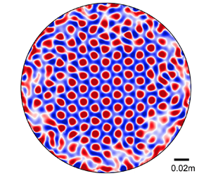
Figure 2. (a–c) Instantaneous vertical vorticity distribution  $\omega /\omega _{std}$, where $\omega _{std}$ is the standard deviation of $\omega$. Results are for the reference cell (a), the square-patterned cell (b) and the hexagon-patterned cell (c), with $\varOmega = 1.12 \times 10^4$ and $\varepsilon = 0.49$. The spacing of the raised cylinders is $\lambda = 14.14$ mm (b) and $17.32$ mm (c). (d–f) Fourier spectra $F(\boldsymbol {k})$ of the vorticity field, determined by $\omega (\boldsymbol {r})$ in the central region of $60 \times 60$ mm $^2$ shown in (a–c), respectively. The arrow in (d) shows the mean radius $k_0$ of the crater-like structure. The arrows in (e) and (f) represent the characteristic wave vectors $\boldsymbol {k}_{f} = \boldsymbol {k}_i$ ( $i = 1,2\ldots$) of the imposed textures. Movies for (a–c) are available (see supplementary movies at https://doi.org/10.1017/jfm.2022.780).
For flow visualization, a particle image velocimetry system is installed on the co-rotating frame. A thin light-sheet powered by a solid-state laser illuminates the seed particles in a horizontal plane at a fluid height  $z = H/4$. Images of the particle are captured through the top sapphire window by a high-resolution camera. Two-dimensional velocity fields are extracted by cross-correlating two consecutive particle images. To investigate the long-term stability of the flow pattern near onset (e.g. figures 2b and 2c), we take image sequences over eight hours at a time interval of 0.5 s.
The experiment is conducted with a constant Prandtl number  $Pr = \nu /{\kappa } = 4.38$ and in the range $2.0 \times 10^6 \le Ra \le 1.0 \times 10^8$ of the Rayleigh number ${Ra} = {\alpha }g{{\rm \Delta} }TH^3/{\kappa }{\nu }$. Here $g$ is the gravitational acceleration, while $\alpha$ and $\kappa$ are respectively the isobaric thermal expansion coefficient and the thermal diffusivity of the fluid. Deionized water is used as the working fluid. Rotating angular velocities of $0.6 \le {\varOmega _{D}} \le 2.0$ rad s $^{-1}$ are used; thus $3.6 \times 10^3 \le {\varOmega } \le 1.2 \times 10^4$. The reduced Rayleigh number, $\varepsilon = ({Ra} - {Ra}_{c})/{Ra}_{c}$, spans the range $- 0.6 \le {\varepsilon } \le 13.5$. The onset value of ${{\rm \Delta} }T_{c}$ for convection is determined from the theoretical prediction using an asymptotic method (Niiler & Bisshopp Reference Niiler and Bisshopp1965), i.e. ${Ra}_{c}({{\rm \Delta} }T_{c}) = a {Ek}^{-4/3}$, with $a = 8.70 - 9.63 {Ek}^{1/6}$ and the Ekman number ${Ek} = \nu /2{\varOmega _{D}}H^2$; and also from the measured intensity of the vorticity field in the cell (see panel c in figure 4). For $\varOmega = 1.12 \times 10^{4}$, the two determinations of ${{\rm \Delta} }T_{c}$ agree to within 0.02 K. The Froude number, ${Fr} = {\varOmega }_{D}^2d/2g$, covers the range $4.4 \times 10^{ - 3} \le {Fr} \le 0.05$.
3. Results and discussions
3.1. Convection patterns
Figure 2 presents the flow patterns at the measured fluid height with  $\varOmega = 1.12 \times 10^4$ and $\varepsilon = 0.49$. When a flat bottom plate is used (i.e. the reference cell without external forcing), the flow fields of the vertical vorticity $\omega (\boldsymbol {r})$ are characterized by columnar vortices, which exhibit stochastic horizontal motions as reported in previous studies (Chong et al. Reference Chong, Shi, Ding, Ding, Lu, Zhong and Xia2020; Ding et al. Reference Ding, Chong, Shi, Ding, Lu, Xia and Zhong2021). Despite their random motion, the vortices maintain approximately a constant distance $\lambda _0 = 13.75{\pm }1.57$ mm from their neighbouring vortices (figure 2a). In the spatial Fourier spectrum $F(\boldsymbol {k})$ of the vorticity field calculated in the central region (figure 2d), a crater-like structure with radius $k_0 = 2{{\rm \pi} }/\lambda _0 (457.1{\pm }52.4$ m $^{-1}$) is apparent, indicating that the vortices are distributed with random orientations but with a preferred spacing. When periodic topographic structures are constructed on the bottom plate, they modulate both the local temperature and the shearing interaction of the fluid with the solid surface, leading to new convection patterns. Figures 2b and 2c show the vorticity fields when the bottom surface is textured with a square and a hexagonal array of cylinders, respectively, with their spacing $\lambda$ chosen close to the intrinsic wavelength of the vorticity field $\lambda _0$. Since the fluid overlying the raised cylinders is relatively hotter than the background fluid at the same fluid height, upwelling vortices, i.e. cyclones when observed in the lower half of the fluid layer (see e.g. Sakai (Reference Sakai1997), King & Aurnou (Reference King and Aurnou2012), for illustrations), tend to form above the cylinders, forming a 1 : 1 commensurate structure with respect to the bottom texture. The downwelling vortices (anticyclones), however, appear in between the raised cylinders. In the square-patterned cell (figure 2b), both the cyclones and anticyclones constitute a regular square lattice. The flow pattern induced by a hexagonal array of cylinders (figure 2c), however, consists of a hexagonal lattice of anticyclones with a cyclone located at the hexagon centre. Such patterns are stationary and persist during the experiment. Figures 2e and 2f present the Fourier spectra of the vorticity fields in the central region of figures 2b and 2c, respectively. In these spectra we see clear peaks located precisely at the wave vectors $\boldsymbol {k}_{f} = \boldsymbol {k}_i$ ( $i = 1,2\ldots$) of the periodically imposed textures. These peaks of $F(\boldsymbol {k})$ are all sharp and their amplitudes are approximately equal, suggesting that regular patterns with prescribed periodicity and symmetry are developed. Near the sidewall region ( $r\,{\ge }\,100$ mm) where the imposed texture is absent, the flow field is time-varying and the vortex dynamics is largely influenced by the retrograde travelling plumes within the region of the boundary zonal flow (de Wit et al. Reference de Wit, Aguirre Guzmán, Madonia, Cheng, Clercx and Kunnen2020; Zhang et al. Reference Zhang, van Gils, Horn, Wedi, Zwirner, Ahlers, Ecke, Weiss, Bodenschatz and Shishkina2020).
3.2. General features of the patterns in the  $k_f - {\varepsilon }$ phase diagram

The observed spatial pattern can be quantified by the radial distribution function  $g(r)$ of the vortices, which is defined as the ratio of the actual number of cyclones lying within an annulus region of $r$ and $r + {\delta }r$, to the expected number for uniform vortex distribution (Chong et al. Reference Chong, Shi, Ding, Ding, Lu, Zhong and Xia2020). Figure 3(a) shows $g(r)$ for cyclonic distribution for various $\varepsilon$ in the square-patterned cell with $\lambda = 14.14$ mm. Near onset ( $\varepsilon = 0.09$), multiple sharp peaks appear in $g(r)$, which are located at distances that match the main and subharmonic wavelengths $r_{ij}$ of the forced square pattern at the bottom plate, fulfilling the condition $r_{ij} = {\lambda }\sqrt {i^2 + j^2}$ (for $i,j = 0,1,2\ldots$ and $i + j\,{\ge }\,1$). With increasing $\varepsilon$, the peak amplitudes in $g(r)$ decrease while the peak widths increase, signifying a less regular flow pattern. The multiple-peak structure is eventually flattened, and $g(r)$ becomes close to a uniform distribution for $\varepsilon \,{\ge }\,4.0$, where we see the vortices exhibit apparent horizontal motions. We examine as well the role of the periodicity of external forcing on the convection pattern. Figure 3(b) presents results for $g(r)$ near onset ( $\varepsilon = 0.49$) for various cylinder spacings $\lambda = 10.00, 14.14, 20.00, 28.28$ mm. We see that multiple peaks still appear at the main and subharmonic wavelengths $r_{ij}(\lambda )$. For $\lambda \,{\ge }\,20.00$ mm, the first peak is found near $r = \lambda _0$, which is associated with the intrinsic wavelength of the flow field. When $\lambda$ is far from $\lambda _0$, the maxima of $g(r)$ become less dominant and $g(r)$ approaches the result of the reference cell.

Figure 3. (a,b) Radial distribution function  $g(r)$ of cyclones in the square-patterned cell. Results are for various $\varepsilon$ with a constant cylinder spacing $\lambda = 14.14$ mm in (a), and for various $\lambda$ with $\varepsilon = 0.49$ in (b). The red, blue and green arrows in (b) denote the main and subharmonic wavelengths $r_{ij}/{\lambda _0}$ of the imposed pattern for $\lambda = 14.14, 20.00$ and $28.28$ mm, respectively. The dotted line in (b) shows the results for the reference cell. (c) Contour plot of the cross-correlation coefficient $C$ of the vorticity field and bottom texture in the $k_f/k_0 - \varepsilon$ phase diagram. Open symbols are data points measured in the square-patterned cell; colour contours are estimated from interpolation between these points. Results are for $\varOmega = 1.12 \times 10^4$.
The degree of matching between the flow pattern and the bottom texture can be evaluated through the cross-correlation coefficient  $C$ of the vorticity field and the bottom texture, defined as $C = {\langle }(\omega (\boldsymbol {r}) - \bar {\omega })(M(\boldsymbol {r}) - \bar {M}){\rangle }/\sqrt {{\langle }(\omega (\boldsymbol {r}) - \bar {\omega })^2{\rangle }{\langle }(M(\boldsymbol {r}) - \bar {M})^2{\rangle }}$, with $M(\boldsymbol {r}) = 0$ (or $- 1$) for the flat (or raised) area representing the bottom surface profile. Angle brackets ${\langle }{{\,\cdot\, }}{\rangle }$ denote a spatial average. Figure 3(c) summarizes the results for $C$ in the square-patterned cell for varying $\varepsilon$ and wave vector $k_{f} = {\vert }\boldsymbol {k}_1{\vert } = {\vert }\boldsymbol {k}_2{\vert }$ of the external forcing. In this phase diagram, we see that $C(k_{f},\varepsilon )$ has a single maximum ( $C\,{\approx }\,0.7$) occurring at ( $k_{m} = 0.97k_0, \varepsilon _{m} = 0.09$), which implies the optimal conditions for pattern selection. In the vicinity of $(k_{m}, \varepsilon _{m})$, the spatial distribution of the vortices closely conforms to the bottom texture. The coefficient $C$ decreases if the control parameters $(k_{f}, \varepsilon )$ deviate from $(k_{m}, \varepsilon _{m})$. The decreasing rate of $C$ with increasing $\varepsilon$ is lowest when a near-resonant external forcing $(k_{f}\,{\approx }\,k_0)$ is chosen. The convection pattern and the imposed texture become essentially uncorrelated (with $C \le 0.1$) when $(k_{f}, \varepsilon )$ are set apart from $(k_{m}, \varepsilon _{m})$. Interestingly, when $k_{f}\,{\approx }\,k_{m}$, $C$ remains well above zero for $\varepsilon < 0$, suggesting that under external forcing, convection sets in with finite amplitude in the subcritical regime.
3.3. Variations of the vorticity field near onset
We measure the time-averaged vorticity modulus  ${\langle }{\vert }{\omega }{\vert }{\rangle }$ in an area of $65.8 \times 54.8$ mm $^2$ at the centre of the cell, while slowly scanning ${{\rm \Delta} }T$ in the near-onset range $-0.4 \le \varepsilon \le 0.4$. Results for ${\langle }{\vert }{\omega }{\vert }{\rangle }(\varepsilon )$ for the reference cell and two forced cells are shown in figure 4. Overall, these data suggest two distinct types of bifurcations when $\varepsilon$ increases from below and crosses zero. The reference cell data reveal a sharp transition from a non-convection state with ${\langle }{\vert }{\omega }{\vert }{\rangle } = 0$ for $\varepsilon \le 0$, to a convection state in which ${\langle }{\vert }{\omega }{\vert }{\rangle }$ increases rapidly for $\varepsilon \,{>}\,0$. For both forced cells, however, ${\langle }{\vert }{\omega }{\vert }{\rangle }$ remains positive for $\varepsilon \,{\ge }-\!0.4$ and grows relatively slowly with increasing $\varepsilon$, suggesting a smooth transition. The three inset panels in figure 4 present the vorticity fields captured in the three cells with approximately the same subcriticality ( $\varepsilon \,{\approx }-\!0.1$). They demonstrate that while the fluid is still quiescent in the reference cell, apparent square and hexagonal lattices of convective vortices have formed in the forced cells.

Figure 4. Bifurcation curves of  ${\langle }{\vert }{\omega }{\vert }{\rangle }(\varepsilon )$ near onset. The circles represent the data of the reference cell. The squares and triangles represent respectively data for the square-patterned cell with $\lambda = 14.14$ mm and the hexagon-patterned cell with $\lambda = 17.32$ mm. Error bars denote the standard deviation. The dotted line shows the fitted square-root law for the reference cell, and the solid lines are the predicted imperfect bifurcation curves for the forced cells. Inset panels: time-averaged vorticity fields of the three cells for $\varepsilon \approx {-}0.1$. Data are for $\varOmega = 1.12 \times 10^4$.
3.4. A theoretical model of the bifurcation dynamics
In an effort to understand the  $\varepsilon$-dependence of ${\langle }{\vert }{\omega }{\vert }{\rangle }$ near onset, we propose a phenomenological Ginzburg–Landau-like model for the convection amplitude $A_j$ of rotating RBC in the presence of external periodic forcing (Kelly & Pal Reference Kelly and Pal1978; Coullet Reference Coullet1986; McCoy Reference McCoy2007; Seiden et al. Reference Seiden, Weiss, McCoy, Pesch and Bodenschatz2008):
 \begin{equation} {\partial}_tA_j = {\varepsilon}A_j + {\xi}_0^2{\nabla}^2A_j - \sum_{i = 1}^ng_0^{ij}|A_i|^2A_j + g_2^j{\delta}_jA_j^{{\ast}m - 1}. \end{equation}
In this model we describe the influence of the imposed bottom texture on the multiple-mode flow pattern by mapping the bottom surface profile to a temperature modulation of the bottom plate (Kelly & Pal Reference Kelly and Pal1978; Seiden et al. Reference Seiden, Weiss, McCoy, Pesch and Bodenschatz2008). The quantity  $g_0^{ij}$ is the nonlinear coupling coefficient between the Fourier modes $i$ and $j$ of the flow pattern (Scheel, Mutyaba & Kimmel Reference Scheel, Mutyaba and Kimmel2010); $n$ is the number of dominant modes, i.e. $n = 2$ (3) for the square (hexagonal) pattern; and $\delta _j = c_jh/H$ represents the strength of the external forcing, with the coefficient $c_j = ({1}/{L_xL_y})\int _{ - L_x/2}^{L_x/2}\int _{ - L_y/2}^{L_y/2}2M(x,y) \cos (2{{\rm \pi} }k_x^j{x}+2{{\rm \pi} }k_y^j{y})\, {\rm d}\kern0.06em x\, {\rm d} y$ representing the bottom surface profile (Kelly & Pal Reference Kelly and Pal1978; Seiden et al. Reference Seiden, Weiss, McCoy, Pesch and Bodenschatz2008). We use an area of $60 \times 60$ mm $^2$
$^2$  $(L_x = L_y = 60$ mm) to evaluate $c_j$, and we obtain $c_j = 0.226$ and 0.172 for the square and hexagonal bottom textures, respectively. The quantity $A_j$ is the normalized complex amplitude, which satisfies the relationship ${\sum _{j=1}^n}{\vert }A_j{\vert }^2 = {(Nu - 1)Ra/Ra}_{c}$ (Cross Reference Cross1980; Cross & Hohenberg Reference Cross and Hohenberg1993), with the Nusselt number ${Nu} = QH/{\lambda }{{\rm \Delta} }T$ representing the global heat transport. Here $Q$ is the heat flux through the fluid layer and ${\lambda }$ is the thermal conductivity of the fluid. The quantity $A_j^{\ast }$ is the complex conjugate of $A_j$. The integer $m$ denotes the degree of resonance, and we consider here resonant forcing ( $k_{f}\,{\approx }\,k_0$ and $m = 1$). The coefficients $\xi _0$ and $g_2^j$ represent the spatial variation of $A_j$ and the degree of imperfection, which depend on $\boldsymbol {k}_{f}$ and $\varOmega$.
In view of the symmetry of the flow patterns shown in figures 2b and 2c, one may reconstruct the square pattern with two plane waves with their characteristic wave vectors ( $\boldsymbol {k}_1,\boldsymbol {k}_2$) perpendicular to each other (figure 2e), and the hexagonal pattern using three wave vectors ( $\boldsymbol {k}_1, \boldsymbol {k}_2, \boldsymbol {k}_3$) equally spaced (figure 2f). Since these convection modes are stationary, with the amplitude of each Fourier mode being equal to that of the others, we have $A_i = A_j$, and the measured amplitude is the superposition of the convection amplitudes in all modes: $A = {\sum _{i = 1}^n}A_i = nA_i$. The coupling coefficient $g_0^{ij} = g_0$ and the imperfection coefficient $g_2^j = g_2$ are set to constants for all modes $(i, j)$.
We consider here a stationary solution for the near-onset flow regime. For each modulation mode the spatial variation of  $A$ is negligible since the flow field is nearly periodic (figures 2b and 2c). Accounting for a shift $\varepsilon _0$ of the onset owing to a local increase of the temperature gradient over the bottom texture (McCoy Reference McCoy2007; Seiden et al. Reference Seiden, Weiss, McCoy, Pesch and Bodenschatz2008) and for each imposed pattern $\boldsymbol {k}_{f}\,{\ne }\,\boldsymbol {k}_0$ (Cross Reference Cross1980), we arrive at an amplitude equation for the forced cells: ${(\varepsilon + \varepsilon _0)}A - g_0{\vert }A{\vert }^2A/n + g_2{\delta } = 0$, with $\delta = \sum _{j = 1}^n{\delta }_j$. When the external forcing is absent, $\delta = 0$ and $\boldsymbol {k}_{f} = \boldsymbol {k}_0$. The amplitude equation for the reference cell is thus reduced to ${\varepsilon }A - g_0^rA^3 = 0$, with $g_0^r$ being the nonlinear coupling constant for the reference cell.
In rapidly rotating RBC, the columnar vortices possess similar spatial profiles of temperature, vertical velocity and vertical vorticity (Portegies et al. Reference Portegies, Kunnen, van Heijst and Molenaar2008; Grooms et al. Reference Grooms, Julien, Weiss and Knobloch2010). The amplitude  $A$ is thus related to the mean vertical vorticity modulus ${\langle }{\vert }{\omega }{\vert }{\rangle }$ through a scale factor $S$,
$S$,  $A = S{\langle }{\vert }{\omega }{\vert }{\rangle }$, yielding the following bifurcation equations for ${\langle }{\vert }{\omega }{\vert }{\rangle }$:
 \begin{equation} (\varepsilon + {\varepsilon}_0^s){\langle}{\vert}{\omega}{\vert}{\rangle} - g_0^sS^2{\langle}{\vert}{\omega}{\vert}{\rangle}^3/2 + g_2^s{\delta}^s/S = 0 \end{equation}
for the square-patterned cell,
 \begin{equation} (\varepsilon + {\varepsilon}_0^h){\langle}{\vert}{\omega}{\vert}{\rangle} - g_0^hS^2{\langle}{\vert}{\omega}{\vert}{\rangle}^3/3 + g_2^h{\delta}^h/S = 0 \end{equation}
for the hexagon-patterned cell, and
 \begin{equation} {\varepsilon}{\langle}{\vert}{\omega}{\vert}{\rangle} - g_0^rS^2{\langle}{\vert}{\omega}{\vert}{\rangle}^3 = 0\end{equation}
for the reference cell. Here the superscripts  $s,h$ denote coefficients for the square and hexagonal patterns, respectively. We fitted the experimental data for ${\langle }{\vert }{\omega }{\vert }{\rangle }(\varepsilon )$ to the theoretical predictions of (3.2)–(3.4) for the forced cells and the reference cell, respectively. In figure 4, both the experimental data and the theoretical curve show clearly the signature of a forward bifurcation near $\varepsilon = 0$ in the reference cell when the external forcing is absent. Meanwhile the pronounced rounding of the transition in the two forced cells suggests an imperfect bifurcation, for which we find the values of the bifurcation terms $g_2^s{\delta }^sS^{-1} = 4.38 \times 10^{-4}(s^{-1})$ and ${g_2^h{\delta }^hS^{-1} = 5.00 \times 10^{-4}}(s^{-1})$. The offsets of the convection onset are found to be $\varepsilon _0^s = 1.0 \times 10^{-3}$ and $\varepsilon _0^h = 1.26 \times 10^{-2}$, signifying that the bottom textures increase the local temperature gradient and destabilize the convection system. Moreover we obtain the coefficient of the coupling terms as $g_0S^2 = (2.60 \times 10^2, 4.16 \times 10^2, 6.81 \times 10^2)(s^2)$ for the reference cell, square-patterned cell and hexagon-patterned cell, respectively.
We consider a dimensionless bifurcation parameter,  $G = \sqrt {g_0}g_2$, which reveals the transitional property of the bifurcation curve ${\langle }{\vert }{\omega }{\vert }{\rangle }(\varepsilon )$ near onset. For the two forced cells we find $G^s = \sqrt {g_0^s}g_2^s = 0.416$, $G^h = \sqrt {g_0^h}g_2^h = 0.530$; both are independent of the scale factor $S$. Although there exists to date no complete theory of near-onset bifurcation for rotating convection with external forcing, the amplitude equation of RBC subject to a spatially periodic modulation has been formulated (Kelly & Pal Reference Kelly and Pal1978; McCoy Reference McCoy2007); these papers show that the external forcing results in an imperfection term with a coefficient $g_2^{\ast } = 0.144$, and a coupling coefficient in the cubic term $g_0^{\ast } = 13.05$, in their chosen units. Therefore, the theoretically predicted value of the bifurcation parameter for non-rotating convection, $G^{\ast } = \sqrt {g_0^{\ast }}g_2^{\ast } = 0.520$, appears close to our results for $G^s$ and $G^h$ for the square- and hexagon-patterned cells in rotating convection. Lastly, the agreement between the experimental and theoretical results shown in figure 4 suggests that the physics of external modulation near the onset of rotating convection is well described by the present Ginzburg–Landau-like model.
4. Concluding remarks
The flow pattern in geostrophic convection is characterized by columnar vortices exhibiting stochastic horizontal motion (see e.g. Noto et al. Reference Noto, Tasaka, Yanagisawa and Murai2019; Chong et al. Reference Chong, Shi, Ding, Ding, Lu, Zhong and Xia2020; Ding et al. Reference Ding, Chong, Shi, Ding, Lu, Xia and Zhong2021). We have shown that when a periodically topographic structure is introduced on the heated surface, these vortex motions can be strictly controlled to form stationary convection patterns with prescribed symmetries. We demonstrate that the new patterns arise through a dynamical process of imperfect bifurcation, with the nature of the bifurcation to finite-amplitude convection well described by a Ginzburg–Landau-like model. It is reported that these coherent vortex structures play a crucial role in heat and mass transport in rotating convection (Veronis Reference Veronis1959; Julien et al. Reference Julien, Legg, Mcwilliams and Werne1999; King & Aurnou Reference King and Aurnou2012) and have significant influence on geophysical and astrophysical phenomena (Balme & Greeley Reference Balme and Greeley2006; Jones Reference Jones2011, et al.). Our findings of a parameter regime in the vicinity of convection onset ( $\varepsilon \le 10$) to manipulate these vortices through topographical forcing may enable a new experimental methodology to control and exploit local heat and energy exchange through rotating flows. There are still experimental challenges in extending investigations of spatial forcing on rotating convection to geophysically relevant ranges of parameters. The richness of patterns in modulated rotating convection observed in this study may stimulate further theoretical and numerical investigations, and contribute to our understanding of non-equilibrium systems constrained by non-uniform boundary conditions.
Supplementary movies
Supplementary movies are available at https://doi.org/10.1017/jfm.2022.780.
Funding
This work was supported by the National Natural Science Foundation of China under grant nos 92152105 and 11772235, the Research Program of the Science and Technology Commission of Shanghai Municipality, and the Fundamental Research Funds for the Central Universities in China.
Declaration of interests
The authors report no conflict of interest.


