


1. Introduction
Shallow flows through arrays of obstacles are ubiquitous in natural and engineered systems, such as flows through patches of aquatic vegetation (Chen et al. Reference Chen, Ortiz, Zong and Nepf2012), groups of bridge piers (Sumer & Fredsøe Reference Sumer and Fredsøe1997), pile foundations (Ball et al. Reference Ball, Stansby, Allison and Strouhal1996; Coulbourne et al. Reference Coulbourne2011) and arrays of tidal stream turbines (Creed et al. Reference Creed, Draper, Nishino and Borthwick2017). Drag on an obstacle array creates a region of low momentum fluid immediately downstream (the wake). Depending on the balance of forces in the wake, the wake can take a variety of different forms. To first approximation, these obstacle arrays can be modelled by a circular array of cylinders, which allows for studying fundamental fluid mechanics of wake structure relevant to practical applications. The wake structure controls the transport of mass and momentum behind these arrays (e.g. Follett & Nepf Reference Follett and Nepf2012; Zong & Nepf Reference Zong and Nepf2012).
Taking flow through a patch of aquatic vegetation as a canonical example, the wake structure was shown to have significant ecological and geomorphological implications. The wake structure has been demonstrated to control the morphology of mobile bed sediments in the lee of aquatic vegetation. Wakes with a von Kármán vortex street were observed to spread sediment towards the wake centreline, whilst wakes without the vortex street spread sediment away from the wake centreline (Follett & Nepf Reference Follett and Nepf2012). Flow passing through the vegetation patch can generate a steady flow region immediately behind the patch with relatively low velocity and turbulence levels (Zong & Nepf Reference Zong and Nepf2012), such that sediment erosion is reduced and fine particle deposition is elevated in the region (Chen et al. Reference Chen, Ortiz, Zong and Nepf2012). The steady wake region, whose scale can vary widely with flow and vegetation characteristics, is therefore a suitable site for the establishment of seeds and is favourable for new plant growth by providing a stable substrate (Follett & Nepf Reference Follett and Nepf2012). Because of this, vegetation patches in channels have been found to propagate predominantly in the downstream direction, forming a streamlined shape extensively observed in the field (Duarte & Sand-Jensen Reference Duarte and Sand-Jensen1990; Gurnell et al. Reference Gurnell, Petts, Hannah, Smith, Edwards, Kollmann, Ward and Tockner2001). These practical implications highlight the importance of understanding the wake structure in shallow flow, in particular if prediction of the wake structure can inform the design of vegetation restoration projects.
A range of parameters has been proposed for classification of wake structure behind an array of cylinders in vertically unbounded flow (without bed). These parameters include the gap ratio G/d (where G is the centre-to-centre distance between the nearest tandem cylinders in a staggered array and d is the cylinder diameter) (Ball et al. Reference Ball, Stansby, Allison and Strouhal1996; Takemura & Tanaka Reference Takemura and Tanaka2007) and the solid volume fraction ( $\phi = ({\rm \pi} /4)n{d^\textrm{2}}$, where n is the number of cylinders per unit area) (Nicolle & Eames Reference Nicolle and Eames2011; Zong & Nepf Reference Zong and Nepf2012). These two geometric parameters describe the local cylinder configuration within the array but without considering the influence of the array size D/d defined by Chang & Constantinescu (Reference Chang and Constantinescu2015) (D is the array diameter).
By varying these geometric parameters, three different wake regimes have been identified (Nicolle & Eames Reference Nicolle and Eames2011; Zong & Nepf Reference Zong and Nepf2012): (i) coupled individual wake (CI), in which the array wake is dominated by individual wakes of the cylinders making up the array; (ii) ‘steady + shedding’ wake (SS), in which a steady wake region occurs behind the array, followed downstream by a von Kármán vortex street; and (iii) vortex street wake (VS), in which a von Kármán vortex street forms immediately behind the array. However, some flows reported in literature cannot be classified into these three regimes. Whilst these unclassified flows do not exhibit a von Kármán vortex street, the array shear layers are unstable with large-scale undulatory motions (Zong & Nepf Reference Zong and Nepf2012; Chang & Constantinescu Reference Chang and Constantinescu2015). It appears that these cases might fall into a fourth regime that requires further investigation, which is one of the motivations for the present work.
The critical values of solid volume fraction and gap ratio defining the same wake transition are inconsistent across different systems. For instance, it was shown by Nicolle & Eames (Reference Nicolle and Eames2011) that the wake transits from regime CI to SS and to VS at  $\phi = 0.05$ and 0.15, respectively. In contrast, the wake transition from regime CI to SS was found in the range of ϕ = 0.05–0.1 by Chang & Constantinescu (Reference Chang and Constantinescu2015) and at ϕ = 0.04 by Zong & Nepf (Reference Zong and Nepf2012). Similarly, wake transition from CI and SS occurred in the range of G/d = 1–2 reported by Takemura & Tanaka (Reference Takemura and Tanaka2007) and distinctly at G/d > 8 reported by Ball et al. (Reference Ball, Stansby, Allison and Strouhal1996). These critical G/d values correspond to ϕ = 0.23–0.91 for Takemura & Tanaka (Reference Takemura and Tanaka2007) and ϕ > 0.01 for Ball et al. (Reference Ball, Stansby, Allison and Strouhal1996) (taking $\phi = (\sqrt 3 {\rm \pi}/6){d^2}/{G^2}$ for their staggered arrays). The difference in the threshold of the same wake transition between different studies indicates that neither $\phi $ nor $G/d$ completely defines the wake structure.
Physically, in vertically unbounded flow, the wake structure behind an array of cylinders depends on the velocity of bleeding flow due to the stabilisation effect of bleeding flow on the wake (Nicolle & Eames Reference Nicolle and Eames2011). This bleeding velocity has been shown to be a function of the dimensionless flow blockage parameter (Chang & Constantinescu Reference Chang and Constantinescu2015):
 \begin{equation}{\varGamma _D} = \frac{{{C_d}aD}}{{(1 - \phi )}},\end{equation}
where a = nd is the frontal area of cylinders within the array per volume, D is the array diameter and  ${C_d}$ is the average drag coefficient of individual cylinders, defined as
 \begin{equation}{C_d} = \frac{F}{{{\textstyle{1 \over 2}}\rho N\,{d}\langle\bar{u}\rangle_d^2}},\end{equation}
in which F is the total drag force acting on cylinders per unit depth,  ${\langle\bar{u}\rangle_d}$ is the spatial average of velocities over the domain occupied by fluids in the array (Eames, Hunt & Belcher Reference Eames, Hunt and Belcher2004), ρ is the fluid density and N is the total number of cylinders within the array. This parameter represents the scaling ratio of two terms in the streamwise momentum equation: the drag on the array elements retarding the flow and the streamwise advection term describing flow deceleration through the array (Rominger & Nepf Reference Rominger and Nepf2011). Importantly, it is seen that ${\varGamma _D}$, defining the blockage of an array to flow, is not only dependent on ϕ but is also governed by ${C_d}$ and the dimensionless array size $D/d$ ((1.1) can be re-written as ${\varGamma _D} = (4{C_d}/{\rm \pi})(\phi /(1 - \phi ))(D/d)$). The incompleteness of using $G/d$ and $\phi $ to define the array-induced flow blockage may explain the inconsistency in existing wake classification approaches based on $G/d$ and $\phi $. The flow blockage parameter has been used to describe the bleeding flow through a submerged cylinder array by Belcher, Jerram & Hunt (Reference Belcher, Jerram and Hunt2003), an infinitely long array of cylinders by Rominger & Nepf (Reference Rominger and Nepf2011) and a finite, circular array by Chang & Constantinescu (Reference Chang and Constantinescu2015). However, the influence of ${\varGamma _D}$ on wake structure behind a cylinder array has not been investigated yet.
When the water depth is small relative to the horizontal scale of the array (‘shallow’), flow shallowness is also physically important in controlling wake structure. The effect of flow shallowness is not well understood for an array of cylinders but it has been explored in more detail for an isolated solid cylinder (for which ϕ = 1,  ${\varGamma _D} = \infty$). The shallowness influences the wake development behind an isolated cylinder in two ways (Chen & Jirka Reference Chen and Jirka1995): (i) it restricts spanwise motions such that the wake structure is largely two-dimensional; and (ii) bed friction acts to suppress the transverse motion of large-scale disturbances such as vortex shedding.
The shallowness effects on the wake structure behind the isolated cylinder can be described by the wake stability parameter:
 \begin{equation}{S_C} = \frac{{{C_f}D}}{h}\textrm{,}\end{equation}
where Cf is the bed friction coefficient and h is the water depth (Ingram & Chu Reference Ingram and Chu1987). This parameter represents the scaling ratio between the energy production from the mean shear and energy dissipation by bed friction in the turbulent kinetic energy equation (Chu, Wu & Khayat Reference Chu, Wu and Khayat1991). Hence, it is a measure of the stabilising influence of bed friction relative to the destabilising influence of transverse shear on the development of wake instabilities downstream of the isolated cylinder.
Extending this wake stability parameter to an array of cylinders is, however, not limited to only quantifying the shallowness influences on wake development downstream of the array because it may also describe the shallowness effect on the bleeding flow that stabilises the wake. For a cylinder array, this wake stability parameter also represents the scaling ratio between the bed friction term and the inertial term in the streamwise momentum equation for the flow diverted around the array (termed ‘diverted flow’) (White & Nepf Reference White and Nepf2007). The bed friction has been shown to impede the faster diverted flow, which in turn increases the velocity of bleeding flow (Creed et al. Reference Creed, Draper, Nishino and Borthwick2017). The increased bleeding velocity will lead to a more stabilised wake (Nicolle & Eames Reference Nicolle and Eames2011). Despite being implied by the energy and momentum conservation, the combined influence of SC on wake structure of an array of cylinders has not been experimentally explored and confirmed.
The wake structure behind an isolated cylinder was found to be solely controlled by wake stability parameter when the depth Reynolds number (where Reh = U∞ h/ν in which ν is the kinematic viscosity and  ${U _{\infty}}$ is velocity upstream of the obstacle) is higher than 1500 (Chen & Jirka Reference Chen and Jirka1995). However, this is not the case for an array of cylinders. The wake stability parameter basically is a relative measure of strength of the transverse shear to the bed shear. For an isolated cylinder, the strength of transverse shear scales on the body diameter D (Ingram & Chu Reference Ingram and Chu1987) that is incorporated in SC. In contrast, for an array of cylinders, the transverse shear strength is determined by the difference between the bleeding flow and diverted flow (Chang & Constantinescu Reference Chang and Constantinescu2015). The strength is not a simple scaling relation with D but is associated with ${\varGamma _D}$ that controls the bleeding velocity. This means that the threshold of SC for the same wake transition should be dependent on ${\varGamma _D}$. Although this argument has not been confirmed by varying ${\varGamma _D}$ systematically, it is, to some extent, supported by the observation with varying ϕ by Wang et al. (Reference Wang, Zhang, Liang and Gan2019). In their study, vortex street was shown behind a cylinder array with ϕ = 0.1 at SC = 0.03 but was absent for the array with ϕ = 0.03 at the same SC value. Note that the two solid volume fractions correspond to two different values of flow blockage parameter $({\varGamma _D} = 1.7,4.9)$.
Considering the findings described above, it is apparent that none of gap ratio, solid volume fraction and wake stability parameter independently provides a universal description about wake structure behind an array of cylinders in shallow flow. This motivates the present study to integrate and reconcile wake classification approaches into one that is consistent across different flow-array systems and different parts of the parameter space for ϕ,  $G/d$ and SC. Applying energy and momentum conservation to the system as described above implies that the wake structure associated with shallow flow through an array of cylinders should be, to first order, controlled by both flow blockage and wake stability parameters ( ${\varGamma _D}$, SC). This combined parameter set contributes to a new integrated, transferable approach for wake classification.
This integrated approach will be validated by a thorough experimental exploration of wake structure across physically important flow conditions that have not been investigated before. Table 1 indicates that existing work has largely focused on flows with SC < 0.01. However, the SC value exceeds 0.01 for many systems of interest. Taking reeds in rivers and seagrasses in oceans as two archetypal examples, the typical patch widths are D ∼ O(1–100 m), with per-volume frontal areas of a ∼ O(0.1–1 m–1) (e.g. Wang & Wang Reference Wang and Wang2007; Kotschy & Rogers Reference Kotschy and Rogers2008; Boulord et al. Reference Boulord, Mei, Tian-Hou, Xiao-Ming and Jiguet2012). For flow depths h ∼ O(0.1–1 m), bed friction coefficients Cf ∼ O(0.001) (Ingram & Chu Reference Ingram and Chu1987; Nezu & Nakagawa Reference Nezu and Nakagawa1993) and average drag coefficients  ${C_d}\sim O(1)$ (Tanino & Nepf Reference Tanino and Nepf2008; Ghisalberti Reference Ghisalberti2009), the two key parameters will therefore have ranges of SC ∼ O(0.01–0.1) and ${\varGamma}_D \sim O(0.1\hbox{--}100)$. Mapping out wake regimes across this practical parameter space will lead to a predictive framework for the wake structure behind an array of obstacles. Replicating existing results concerning wake structure in subsets of this parameter space will be a starting point for developing this framework.
Table 1. Summary of existing studies that investigated the wake structure behind obstacle systems. Note: Exp, laboratory experiment; Num, numerical simulation.

Designing high-fidelity physical and numerical modelling studies across the full practical parameter space of  $\varGamma_{D}$ and $S_{C}$ has proven challenging. In shallow water systems, the horizontal scale of the obstacle is significantly larger than the water depth. Laboratory-scale modelling of these shallow systems while keeping the channel wall blockage ratio (D/W) small enough to have negligible influence necessitates an experimental flume facility that is very wide and capable of generating flow with very small water depth (even down to 1 cm). Such flumes are not commonly available. Numerical modelling of flow through an array of cylinders in vertically unbounded flow requires resolving both the wakes of individual cylinders within the array and the wake behind the array, which is computationally demanding (He Reference He2023). When considering shallow flow, the presence of the bottom bed imparts both dynamic (no slip) and kinematic (no flux) restrictions on the flow, resulting in a three-dimensional (3-D) flow. This bed-induced three dimensionality makes the numerical simulations of shallow flow through an array of cylinders much more computationally expensive.
Motivated by the apparent gap in existing data, together with the prevalence of shallow waters in natural and engineered systems and the need for further understanding of shallow wakes, this study explores the controlling influence of  ${\varGamma _D}$ and SC on shallow wake structures for arrays of cylinders. By combining the present experimental results with existing work, this study aims to: (i) allow prediction of the wake regime for any given circular array of cylinders in shallow flow; (ii) understand instantaneous and time-averaged flow fields within each wake regime; and (iii) reveal the underlying physical mechanisms governing transitions between wake regimes, and their dependence upon ${\varGamma _D}$ and SC.
2. Experimental methods
2.1. Shallow flow facility and model set-up
Experiments were conducted in a recirculating glass flume with a testing section of width (W) 1.85 m, length 6.0 m and maximum depth 0.35 m (figure 1a). An array of polycarbonate flow straighteners and sponges were installed at the inlet of the flume to create uniform unidirectional incident flow.

Figure 1. (a) Schematic diagram (plan view) of the experimental set-up; (b) photograph of a large array (D = 41 cm) in the flume and dye injection system, taken by camera A; (c) photograph of a small array (D = 16 cm) in a narrow channel created by an acrylic splitting plate; (d) photograph of the piezometer set-up. The velocity measurement locations for the transverse profiles (I, red hollow square), point sampling (II, green solid circle), streamwise profile (IV, blue solid square) described in § 2.3 are sketched in panel (a).
To map out wake regimes across the practical parameter space of  ${\varGamma _D}$ and SC, 71 large arrays of acrylic clear circular cylinders with d = 1.0 cm and D = 42.5 ± 1.5 cm were tested. The cylinders were organised in a staggered arrangement and extended from the flume bed through the water surface (figure 1b). Individual cylinders were held in place by a perforated acrylic plate above the water surface. The channel blockage ratio of the flume (D/W) was approximately 22 %. The ambient velocity ${U _{\infty}}$ was maintained at 10.0 cm s−1. The flow depth h ranged from 1 to 11 cm, and the depth Reynolds number Reh ranged from 1000 to 11 000.
As wake stability parameter not only varies with the flow depth but also with the array diameter, there is a need to confirm that the classification of wake regimes based on these large arrays (with virtually constant D) is independent of the array size. To do this, the wake structure is compared between six pairs of arrays, each of which has the same values of  ${\varGamma _D}$, SC and d but different dimensionless sizes (D/d). It will be shown in § 3.1.2 that these six pairs of cases locate near the transition boundaries between different regimes. In this comparison, to keep the channel wall ratio D/W constant, for these experiments with small arrays, an acrylic splitting plate was put in the flume to form a new channel with smaller width (see figure 1c).
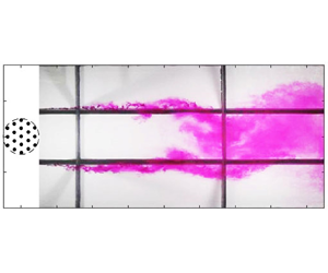
The bed friction coefficient Cf embedded in SC was estimated based on the Blasius equation  ${C_f} = 0.056/Re_h^{0.25}$ (Chow Reference Chow1959) for a smooth wall. Following Chen & Jirka (Reference Chen and Jirka1995), the estimated values were checked by measuring fractional change in water elevation for small water depth (1–2.1 cm) with a piezometer (see figure 1d). Two piezometer tubes were installed 400 cm apart (in the streamwise direction) and 20 cm away from the channel wall to measure the frictional change across these two locations. The 400 cm length covers approximately a 10D wake length in this study. A fixed Canon camera was used to obtain frames of the water levels in the piezometer tubes. KeystoneTM Rhodamine dye in magenta was added into the two tubes to illuminate the water columns. The fractional change in water depth $\mathrm{\Delta }h$ (hence streamwise pressure gradient) between the two locations was calculated using image pixels. Based on momentum balance between the bed shear and the pressure gradient, the bed friction coefficient can be experimentally calculated and compared with the predictions from the Blasius equation (see table 2).
Table 2. Comparison between the measured and predicted (by Blasius equation) bed friction coefficients. Here,  $\Delta h$ is the frictional change in water depth over 400 cm streamwise length, and h is the depth of incident flow at the upstream end of the testing section.

Table 2 reveals that the Blasius equation predicts Cf to within 5 % of the measured values even for the lowest water depth  $(h = \textrm{1}\textrm{.0}\ \textrm{cm)}$. This validates the use of the Blasius equation in estimating Cf across the studied range of $\textrm{1}\textrm{.0} \le h \le \textrm{11}\textrm{.0}\ \textrm{cm}$ (92 % of cases in this study are in the range of $h \ge 1.5\ \textrm{cm}$). This is consistent with Chen & Jirka (Reference Chen and Jirka1995), where the similar relation of Moody friction diagram was found to be valid for a water depth as low as 1.0 cm. The small depth change ratio, $\Delta h/h \le 19.3\,\%$, suggests that the water depth remains virtually invariant along the wake for $h \ge \textrm{1}\textrm{.0}\ \textrm{cm}$. Hence, the wake stability parameter defined based on the incident flow depth is representative (to within 19.3 %) of that over the entire wake region (0 < x < 10D).
The average drag coefficient Cd embedded in  ${\varGamma _D}$ was estimated by the method proposed by He et al. (Reference He, Draper, Ghisalberti, An and Branson2023). Specifically, based on the knowledge of the array geometry and the depth and velocity of the incident flow, the average drag coefficient can be calculated by running an iterative solution between the actuator disc theory (Garrett & Cummins Reference Garrett and Cummins2007) and the empirical drag model (Tanino & Nepf Reference Tanino and Nepf2008).
2.2. Experimental methods
Flow visualisation through dye injection was used to classify wake regimes. The wake classification will be detailed in § 3.1. A dye injection system (figure 1b) was used with a mixture of KeyacidTM Rhodamine WT liquid in magenta (Keystone company, Item ID: 703-010-27), full cream milk (Brownes Dairy, Australia) and 100 % ethanol (Chem-Supply company) that was injected as the flow tracer at two locations (x/D, y/D) = (−0.5, ± 0.5) (figure 1a). The ratio of the volume between the milk, dye and ethanol was approximately 11 : 1 : 2 to match the density of the ambient fluid. The fattiness of milk apparently retarded diffusion of the dye solution into the ambient bulk of water to stabilise the dye filaments, and at the same time, the high reflectivity of the milk particles provided high visibility. A syringe pump was used to inject the dye steadily through a needle of inner diameter equal to 0.8 mm at mid-depth, with an injection velocity matching the local mean flow velocity.
Dye streaks were recorded with three 4K Panasonic cameras at a frame rate of 25 Hz, located outside of the flume and facing inwards towards the flume (see figure 1a). Cameras A and B, facing upstream and downstream, respectively, and camera C (side-looking) provide visualisation of the near wake of the array. Due to the wide range of the array wake and limitation of facility, it is difficult to set the cameras in a top-down view while covering the whole wake. Hence, all the cameras captured the wake structure in oblique views. The resultant oblique images were transformed into plan (top-down) view images through two-dimensional perspective transformation (using inbuilt transformation functions ‘fitgeotrans’ and ‘imwarp’ in MATLAB). To obtain images that clearly defined the wake structure, light diffusion films were placed on the underside of the glass flume base, with LED white lights positioned underneath the flume to illuminate the dye through the light diffusion film (figure 1b). Markers were put on the four corners of the flume to help establish the cartesian coordinate system on the image for further statistical image analysis.
The statistical image analysis was based on the distribution of the green intensity in pixels G(x, y) (in RGB colour, with a maximum of 255) in the wake. Note that, in the RGB colour system, magenta is a secondary colour, made by combining equal amounts of red and blue colours at a high intensity. In this system, magenta is the complementary colour of green, and combining green and magenta colours will create the white colour. Therefore, the dye absorbed white light over the green wavelength range in the light spectrum such that G(x,y) is qualitatively representative of the local dye concentration. The temporal variation of G(x,y) is indicative of the local intensity of coherent motions, which may be quantified using a coefficient of variation as
 \begin{equation}{C_V} = \frac{{{\sigma _G}}}{\mu }\textrm{,}\end{equation}
where  ${\sigma _G}$ is the temporal standard deviation of G(x, y) and μ is the time mean of G(x,y).
Videos were recorded throughout each test, but only the last 100 seconds were used for the image analysis, covering at least five array-scale vortex shedding periods. Taking case H1 as an example (table 3),  ${\sigma _G}$ sampled at (x/D, y/D) = (3, 0) converged after 45 seconds such that $({\sigma _{G.t}} - {\sigma _{G.t + \Delta t}})/\Delta t < 0.4\,\%$ (figure 2a), suggesting a sampling length of 100 seconds was sufficient for statistical convergence.
Table 3. Experimental conditions employed in this study. Testing cases numbered from ‘79’ to ‘83’ represent the dye visualisation cases without array models. Cases with numbered text (e.g. ‘A1’) are those for which wake velocity fields were measured and roman numeral (e.g. ‘I’) denotes the type of velocity measurement.


Figure 2. Variations of temporal standard deviation of (a) green colour intensity  $({\sigma _G})$ and (b) transverse velocity $({\sigma _v})$ with sample length (t) in case H1 (table 3). The horizontal axis t represents the width of a time window (starting from zero) over which ${\sigma _G}$ and ${\sigma _v}$ were calculated. The convergence of ${\sigma _G}$ at a time of 45 seconds and of ${\sigma _v}$ at a time of 260 seconds suggests that sampling periods of 100 and 300 seconds for data from the flow visualisation and velocity measurements, respectively, met statistical convergence.
The evolution of dye streaks was visualised first without the array models to allow comparison with the rate of spread of dye streaks in the presence of the arrays. It was observed that the dye streaks in the empty flume largely remained parallel without merging as they advected downstream (figure 3). The lateral spreading of the dye streaks visible in figure 3 was induced by turbulent diffusion associated with background turbulence.

Figure 3. Evolution of dye streaks in the flow (h = 7 cm) with no array. (a) Instantaneous streak structure; (b) the spatial distribution of CV. The array diameter D used for normalisation is equal to 43 cm. There is lateral spreading of dye streaks due to ‘background’ diffusion, which will be used as a point of comparison for dye streaks in the presence of cylinder arrays.
Velocity measurement was undertaken to help characterise each wake regime. A Sontek two-dimensional side-looking acoustic Doppler velocimeter (ADV) was used to measure the velocity components u(t) and v(t), at mid-depth, in the streamwise (x) and transverse (y) directions, respectively. The ADV works in water depths down to 2 cm. In shallow flow, the velocity measured at mid-depth is a good representation of the depth-average velocity (White & Nepf Reference White and Nepf2007). At each measurement location, the velocity was sampled for 5 mins at a frequency of 25 Hz. As an example, the standard deviation of v(t)  $({\sigma _v})$ sampled at (x/D, y/D) = (3, 0) was converged at a length of 260 seconds after which $({\sigma _{v.t}} - {\sigma _{v.t + \Delta t}})/\Delta t < 2\,\%$ for case H1 (see figure 2b), suggesting the velocity sample duration (300 s) was statistically sufficient. Measurement durations of 600 and 1200 s were required in certain cases to examine the strongly oscillating near wake flow (x/D = 1) of regime VS and the intermittent velocity oscillations of regime KH (introduced later), respectively. Each velocity record was decomposed into time-averaged $(\bar{u},\bar{v})$ and fluctuating components (u′, v′). The turbulence intensity in the ambient flow was calculated as $\sqrt {\overline {{{u^{\prime}}^2}} } /{U_\infty }$, which was typically less than 3 %. Spectra of transverse velocity were used to examine oscillations in the wake; all spectra were smoothed using a Parzen window of width 10. The continuous wavelet transform in MATLAB was used to obtain the spectrogram of v'(t), to examine the variation of oscillation frequency with time.
2.3. Test matrix
The testing conditions for all cases are detailed in table 3. In total, flow visualisation was performed across 78 experimental cases to assess the variation of wake structure across the parameter space. Among these, detailed velocity measurements were undertaken in 22 cases (table 3) to achieve the following five objectives:
(I) to investigate the evolution of array shear layers, five transverse profiles were measured along x/D = 1.0, 3.0, 5.0, 7.0 and 8.5, respectively, for 14 cases. Each transverse profile was sampled from y/D = 0 to 1.6, which included 20 data locations, on average;
(II) to quantify the bleeding flow, velocities at (x/D, y/D) ≈ 0.5 were measured;
(III) to confirm the wake classification by flow visualisation, point measurements at (x/D, y/D) = (7, 0.5), (8.5, 0.5) and (8.5, 0) were collected in some cases near the regime transition boundaries;
(IV) to quantify the length of the steady wake region, velocities along the line of y/D = 0.05 were measured from x/D = 0.5 to 8.5 with high resolution in case F1;
(V) to confirm that the array-scale wake structure is independent of array size, the wake profiles for the small arrays were measured at x/D = 1.0 for comparison to those of large arrays.
The sample locations for I, II and IV are sketched in figure 1(a) as typical examples for the transverse profile, streamwise profile and point measurement, respectively. Each type of velocity measurement is denoted by I, II, III, IV, V in table 3, respectively.
3. Results
3.1. Wake regimes in shallow flow through an array of cylinders
3.1.1. Wake classification
By varying flow blockage and wake stability parameters, four wake regimes are observed behind an array of cylinders in the present experimental program: (i) vortex street wake (VS); (ii) ‘steady + shedding’ wake (SS); (iii) Kelvin–Helmholtz instability wake (KH); and (iv) coupled individual wake (CI).
Figure 4 illustrates the key flow characteristics in each wake regime. The first column shows a snapshot of dye streaks to visualise the instantaneous wake structure (see also the supplementary movies 1–5 available at https://doi.org/10.1017/jfm.2024.338), the second column presents CV to indicate the time-averaged wake structure and the third column plots the power spectral density of the transverse velocity at (x/D, y/D) = (8.5, 0.5).

Figure 4. Wake regimes are well distinguished by the instantaneous wake structure (snapshot of dye streaks), the time-averaged flow structure (field of CV) and power spectral density (Svv) of transverse velocity. The incoming flow is directed upwards. Transverse velocities v for calculating the spectra were sampled at (x/D, y/D) = (8.5, 0.5). The four rows present (in order) cases H1, F1, C1 and A1. The steady wake region in panel (e) is roughly indicated by the black arrow. The series of KH vortices formed in the array shear layer in regime KH in panel (g) is marked by grey arrows.
Regime VS is characterised by a classical von Kármán vortex street formed immediately behind the array (figure 4a). The time-averaged wake structure behind the cylinder array (figure 4b) is similar to the classical wake of a single solid cylinder (Zdravkovich Reference Zdravkovich1997). At any given streamwise location, the value of CV is higher near the wake boundaries than along the wake centreline. Near the wake boundaries, von Kármán vortices continuously entrain the ambient uncoloured fluid into the wake, leading to a sharp change in temporal variation of colour intensity CV from nearly zero to very high values. The von Kármán vortex street behind the cylinder array creates a sharp peak in the spectrum of transverse velocity (figure 4c). The corresponding array Strouhal number (defined as  $S{t_D} = fD/{U_\infty }$) for the case shown is 0.23, which is close to the value $(S{t_D} \approx 0.2)$ of an isolated solid cylinder in a vertically unbounded flow (Sumer & Fredsøe Reference Sumer and Fredsøe1997). Cylinder arrays in the VS regime thus behave similarly to a single solid obstacle in terms of the wake structure.
The ‘steady + shedding’ wake (SS) is characterised by a steady wake region attached behind the array, followed downstream by a von Kármán vortex street. The two array shear layers remain stable in the steady region, before interacting to result in the vortex street downstream. The merging of the dye streaks at the wake centreline (at x/D ≈ 5 in figure 4d) coincides with the end of the steady wake region, as demonstrated by Zong & Nepf (Reference Zong and Nepf2012). The steady wake region is delineated approximately by a region of nearly zero CV in figure 4(e). The vortex street is associated with a sharp peak in the spectrum at StD = 0.21 (figure 4f), which is again similar to that of a single solid cylinder. The formation of a steady wake region immediately downstream of the array is the key feature that differentiates regime SS from regime VS.
The regime KH is identified by the occurrence of a Kelvin–Helmholtz (KH) instability in the array shear layers, through flow visualisation and analysis of the velocity spectrum (described in more detail in § 3.1.3). The array-scale KH vortices (grey arrows in figure 4g) are distinctly different from those in regimes SS and VS in four ways:
(i) the two dye streaks do not mix together at the location where the vortices are initially formed, suggesting the vortices are not generated through the direct interaction between the two shear layers, i.e. vortex shedding;
(ii) the rows of coherent vortices within each array shear layer are not shed from alternating sides of the array (see also the online supplementary movie 3), which indicates that there is minimal temporal correlation between the coherent structures across the two shear layers. This is distinct from that observed in the SS regime where the von Kármán vortices are shed alternately from either side of the array (supplementary movie 2);
(iii) at a given streamwise location, the KH vortices are barely perceptible within either array shear layer at some instants, whereas at other instants, discrete KH vortices had developed in the shear layer (see supplementary movies 3 and 4). This indicates the irregular generation of coherent vortices in array shear layers;
(iv) the frequency content of the wake is different. In contrast to the narrow-banded peak in regimes SS and VS (figure 4c,f), a broadband peak is detected within the array shear layers in the KH regime (figure 4i). The broadband peak, defined as the range in which the power spectral density is larger than 20 % of its maximum, is in the range of approximately $0.16 < fD/{U_\infty } < 0.41$. The broadband peak is indicative of a KH instability in shear flows with a convective nature (Cardell Reference Cardell1993; Prasad & Williamson Reference Prasad and Williamson1997; White & Nepf Reference White and Nepf2007).

In the coupled individual wake (CI), the wakes from the elements of the array are the dominant flow feature in the array wake. The array shear layers still exist in this regime, but they are stable, such that no KH instability or vortex shedding occurs. This is indicated by the similarity of downstream evolution of dye streaks to that of the case without the array (see figures 3a and 4j). The dye streaks expand in the transverse direction smoothly downstream, without rolling up into any coherent vortex structures (figure 4j). The CV value is high near the array and decreases along the wake for regime CI (figure 4k), which is indicative of lower lateral mixing rate downstream and hence no instability developing in the array shear layers in regime CI. The stabilisation of the wake flow is also confirmed by the velocity spectrum, with no identifiable dominant frequency across the entire frequency range (figure 4l).
The differences in the dye streak pattern, spatial CV distribution and spectrum between these four regimes demonstrate the generation of stable array shear layers in regime CI and unstable array shear layers creating coherent vortex structures in regimes KH, SS and VS. A summary of principal features for these four regimes is given in table 4, together with a schematic of the wake structure for each regime.
Table 4. Characteristic flow features of the four wake regimes behind an array of cylinders. Dashed circle represents the edge of a cylinder array, and the incident flow points upwards. Shear layers are considered ‘unstable’ when they generate coherent vortex structures.

3.1.2. Controlling influence of ${\varGamma _D}$ and SC on wake structure

The wake flow regimes observed behind 71 large arrays of cylinders  $(D/d \approx 42.5)$ in shallow flow are mapped out in the ( ${\varGamma _D}$, SC) parameter space in figure 5 (solid symbols), combined with existing data (hollow symbols). From the bottom-right corner to the top-left corner of the ${\varGamma _D}\unicode{x2013} {S_C}$ plane, the wake structure varies from a vortex street wake (VS) to a ‘steady + shedding’ wake (SS), then to a Kelvin–Helmholtz instability wake (KH), and finally to a ‘coupled individual wake’ (CI). This indicates that increases in SC and reductions in ${\varGamma _D}$ tend to suppress the generation of large-scale coherent vortex structures, resulting in more stable wakes.

Figure 5. Separation, in the  ${\textrm{S}_C}\unicode{x2013} {\varGamma _D}$ parameter space, of wake regimes in flows through an array of cylinders. Filled and unfilled markers represent data from this work and previous studies, respectively. Six filled symbols with black edges represent the pairs of cases tested with arrays of both large and small dimensionless array sizes (D/d). The dashed ellipses denote two cases with close values of ${\varGamma _D}$ or SC, but with an approximately 50 % difference in D/d. This chart shows that a wake transition can be caused by variation of either ${\varGamma _D}$ or SC and allows prediction of the wake regime behind an array of cylinders.
Figure 5 shows that data points generated with these large arrays and compiled from the literature, associated with each regime, cluster together within the parameter space. Data points of each regime are separated, forming clear boundary lines between them (as delineated by dashed lines). This clear separation suggests that the wake structure is, to first order, controlled by flow blockage and wake stability parameters, as hypothesised in § 1.
The curved regime boundaries between regimes implies that the wake structure behind a cylinder array depends on both  ${\varGamma _D}$ and SC nonlinearly. With increasing SC, the regime boundary lines become increasingly horizontal (figure 5). This indicates that wake transition depends increasingly on SC as it increases. Figure 5 suggests that there is an upper limited for SC ≈ 0.6 above which only regime CI is found. This is expected as for ${S_C}\mathrm{\ \mathbin{\lower.3ex\hbox{$\buildrel> \over {\smash{\scriptstyle\sim}\vphantom{_x}}$}}\ }0.6$ the wake flow is fully stabilised without any oscillation for an isolated cylinder (Chen & Jirka Reference Chen and Jirka1997). The isolated cylinder, however, has much stronger shear layers than the cylinder array (demonstrated later in § 4.2) and, unlike the porous array, there is no stabilising influence of bleeding flow on the wake. This suggests that SC ≈ 0.6 is conservative for the cylinder array, above which all the instability associated with array shear layers will be completely suppressed. Increasing ${\varGamma _D}$ can have a similar effect to decreasing SC in causing transitions between regimes. Because of the nonlinear dependency, it is difficult to collapse ${\varGamma _D}$ and SC down to one single parameter that defines the wake structure.
As bleeding flow has controlling influence on the wake structure (Wood Reference Wood1967; Zong & Nepf Reference Zong and Nepf2012; Chang & Constantinescu Reference Chang and Constantinescu2015), especially at low wake stability parameter, the shape of the boundary lines between different regimes can be interpreted by scaling terms in the momentum equation. Within the array, the time-mean flow in the streamwise direction is governed by the following equation:
 \begin{equation}\bar{u}\frac{{\partial
\bar{u}}}{{\partial x}} + \bar{v}\frac{{\partial
\bar{u}}}{{\partial y}} =- \frac{1}{\rho }\frac{{\partial
\bar{p}}}{{\partial x}} - \frac{{{C_d}a}}{{2(1 - \phi )}}\bar{u}{({\bar{u}^2} +
{\bar{v}^2})^{1/2}} - \frac{{{C_f}}}{{2h}}{ \bar{u}({\bar{u}^2} +
{\bar{v}^2})^{1/2}},\end{equation}
\begin{equation}\bar{u}\frac{{\partial
\bar{u}}}{{\partial x}} + \bar{v}\frac{{\partial
\bar{u}}}{{\partial y}} =- \frac{1}{\rho }\frac{{\partial
\bar{p}}}{{\partial x}} - \frac{{{C_d}a}}{{2(1 - \phi )}}\bar{u}{({\bar{u}^2} +
{\bar{v}^2})^{1/2}} - \frac{{{C_f}}}{{2h}}{ \bar{u}({\bar{u}^2} +
{\bar{v}^2})^{1/2}},\end{equation}
where  $\bar{p}$ is the time-mean pressure. Similarly, the diverted flow in the streamwise direction at either side of the array is controlled by
 \begin{equation}\bar{u}\frac{{\partial
\bar{u}}}{{\partial x}} + \bar{v}\frac{{\partial
\bar{u}}}{{\partial y}} =- \frac{1}{\rho }\frac{{\partial
\bar{p}}}{{\partial x}} - \frac{{{C_f}}}{{2h}}{\bar{u}({\bar{u}^2}
+
{\bar{v}^2})^{1/2}}.\end{equation}
\begin{equation}\bar{u}\frac{{\partial
\bar{u}}}{{\partial x}} + \bar{v}\frac{{\partial
\bar{u}}}{{\partial y}} =- \frac{1}{\rho }\frac{{\partial
\bar{p}}}{{\partial x}} - \frac{{{C_f}}}{{2h}}{\bar{u}({\bar{u}^2}
+
{\bar{v}^2})^{1/2}}.\end{equation}
When the array flow blockage ( ${\varGamma _D}$) is low, it is normally assumed that the pressure gradient $(\partial \bar{p}/\partial x)$ approaches zero and hence the pressure terms in both (3.1) and (3.2) drop out; if the array flow blockage is high, the flow will become fully developed with the streamwise pressure gradient in the array equal to that in the diverted flow, and hence the pressure gradients in (3.1) and (3.2) are cancelled out (Rominger & Nepf Reference Rominger and Nepf2011). To first approximation, the fraction of flow passing through the array (bleeding flow velocity, ${\bar{u}_b}$) therefore depends on the ratio between the flow resistances in the array and in the diverted flow as
 \begin{equation}\frac{{{{\bar{u}}_b}}}{{{U_\infty
}}} = f\left( {\frac{{ -
\dfrac{{{C_f}}}{{2h}}{{\bar{u}({{\bar{u}}^2} +
{{\bar{v}}^2})}^{\frac{1}{2}}}}}{{ - \dfrac{{{C_d}a}}{{2(1 - \phi )}}{{\bar{u}({{\bar{u}}^2} +
{{\bar{v}}^2})}^{\frac{1}{2}}} -
\dfrac{{{C_f}}}{{2h}}{{\bar{u}({{\bar{u}}^2} +
{{\bar{v}}^2})}^{\frac{1}{2}}}}}}
\right)\!.\end{equation}
\begin{equation}\frac{{{{\bar{u}}_b}}}{{{U_\infty
}}} = f\left( {\frac{{ -
\dfrac{{{C_f}}}{{2h}}{{\bar{u}({{\bar{u}}^2} +
{{\bar{v}}^2})}^{\frac{1}{2}}}}}{{ - \dfrac{{{C_d}a}}{{2(1 - \phi )}}{{\bar{u}({{\bar{u}}^2} +
{{\bar{v}}^2})}^{\frac{1}{2}}} -
\dfrac{{{C_f}}}{{2h}}{{\bar{u}({{\bar{u}}^2} +
{{\bar{v}}^2})}^{\frac{1}{2}}}}}}
\right)\!.\end{equation}Simplifying (3.3) gives
 \begin{equation}{f^{ - 1}}\left( {\frac{{{{\bar{u}}_b}}}{{{U_\infty }}}} \right) = \frac{{{S_C}}}{{{S_C} + {\varGamma _D}}}.\end{equation}
Rearranging (3.4) yields
 \begin{equation}{S_C} = \frac{{{f^{ - 1}}\left( {\dfrac{{{{\bar{u}}_b}}}{{{U_\infty }}}} \right)}}{{1 - {f^{ - 1}}\left( {\dfrac{{{{\bar{u}}_b}}}{{{U_\infty }}}} \right)}}{\varGamma _D}.\end{equation}
With a critical value of  ${f^{ - 1}}({\bar{u}_b}/{U_\infty })$, the relationship in (3.5) for the bleeding flow can be mapped out into the SC– ${\varGamma _D}$ space, which sets a boundary line between the two adjacent regimes in the regime chart in figure 5. Clearly, for a constant value of ${f^{ - 1}}({\bar{u}_b}/{U_\infty })$, SC is proportional to ${\varGamma _D}$ and hence the boundary line between each of the two adjacent regimes (e.g. CI, KH) should be a straight line in the log-scale regime chart. This is valid only when the wake stability parameter is low and the influence of bleeding flow dominates the wake transition. For a high value of SC, the bed friction not only affects the bleeding flow velocity (as described in (3.5)) but also plays an important role in suppressing the instabilities in the far wake. This suppression effect of bed friction on the instabilities has been demonstrated for the single mixing layer (Chu et al. Reference Chu, Wu and Khayat1991) and the wake behind an isolated cylinder (Chen & Jirka Reference Chen and Jirka1995, Reference Chen and Jirka1997) in shallow water. This suppression effect will be demonstrated for an array of cylinders later in § 4.1.2. With this bed friction effect on wake instabilities, the boundary lines between adjacent regimes should deviate downwards from linear lines for a high value of SC.
These scaling arguments are consistent with the experimental observations. Figure 5 shows that the boundary lines between different regimes are close to linear at  ${S_C} \mathrm{\ \mathbin{\lower.3ex\hbox{$\buildrel< \over {\smash{\scriptstyle\sim}\vphantom{_x}}$}}\ }0.1$, whereas boundary lines increasingly deviate downwards from linear lines to be horizontal with the increase of SC for ${S_C} \mathrm{\ \mathbin{\lower.3ex\hbox{$\buildrel> \over {\smash{\scriptstyle\sim}\vphantom{_x}}$}}\ }0.1$. This indicates that the wake transitions for ${S_C} \mathrm{\ \mathbin{\lower.3ex\hbox{$\buildrel< \over {\smash{\scriptstyle\sim}\vphantom{_x}}$}}\ }0.1$ and ${S_C} \mathrm{\ \mathbin{\lower.3ex\hbox{$\buildrel> \over {\smash{\scriptstyle\sim}\vphantom{_x}}$}}\ }0.1$ are primarily governed by the array-induced flow blockage and shallowness, respectively.
The regime chart in figure 5 is initially established by varying the water depth while keeping the array diameter virtually constant  $(D \approx 42.5\ \textrm{cm)}$ since it is more effective to change SC through varying h rather than D. This means that the observed wake transition along the SC-axis of the regime chart reflects the influence of limited water depth rather than the complete range of SC. To further demonstrate the controlling influence of SC and ${\varGamma _D}$, here, the dependence of this regime chart on the array size $D/d$ is explored. In particular, the model array diameter was halved in the particular cases that fell near regime boundaries (symbols with black edge in figure 5), while maintaining the same values of SC, ${\varGamma _D}$ and d (cases ‘72–77’ listed in table 3).
Flow visualisation shows that halving the array diameter has minimal impact on the wake structure. In total, six pairs of scenarios in the neighbourhood of regime boundaries were examined (see table 5). It is seen that flows with the same governing parameter set ( ${\varGamma _D}$, SC) but with an approximately 50 % difference in D/d display the same wake form. This independence of wake structure on the dimensionless array size is also confirmed through measurement of the transverse profile of mean velocity in the wake. There is good agreement of transverse profiles of streamwise velocity $(\bar{u}/{U_\infty })$ at x/D = 1 between the large and small arrays with the same values of ${\varGamma _D}$ and SC (see figure 6).
Table 5. Comparison of visualised wake regimes for pairs of cases with the same values of  ${\varGamma _D}$ and SC, but different size (D/d). Note that the cylinder diameters for all cases are d = 1 cm. In all pairs, there is no change of wake form when the array diameter is halved, confirming that the wake structure is primarily controlled by ${\varGamma _D}$ and SC.


Figure 6. Comparison of wake profiles of  $\bar{u}/{U_\infty }$ at x/D = 1 between the cases of large and small D/d values. The pair of cases in each panel have the same values of ${\varGamma _D}$ and SC, but an approximately 50 % difference in D/d. There is negligible difference between the pair of velocity profiles in panels (a)–(d), demonstrating the independence of wake structure on the array size.
The independence of this regime chart on dimensionless array size is also confirmed by the consistency of wake regimes between different studies for the same values of  $\varGamma_{D}$ and $S_{C}$. Table 6 summarises the broad range of dimensionless array size (D/d), Reynolds numbers defined based on the element diameter (Red), array diameter (ReD) and water depth (Reh) for independent studies. Despite large difference in values of D/d, Red, ReD and Reh, near the transition boundaries, the data points with close values of ${\varGamma _D}$, SC lie in the same wake regimes (CI, KH, SS). For instance, the data points from the present study and those from existing work (Zong & Nepf Reference Zong and Nepf2012; Chang et al. Reference Chang, Constantinescu and Tsai2017; Wang et al. Reference Wang, Zhang, Liang and Gan2019) (marked with dashed ellipses in figure 5) with close values of ${\varGamma _D}$ and SC all share the same wake regimes despite their D/d values varying by a factor of two. In summary, the similarity of wake structures between arrays with the same values of ${\varGamma _D}$ and SC but different values of D/d (in the range $3.5 < D/d < 81.9$) demonstrates the controlling influence of flow blockage and wake stability parameters on wake structure, and thus the insensitivity of this regime chart to array size.
Table 6. Summary of array size (D/d), Reynolds number defined based on element diameter (Red), array diameter (ReD) and water depth (Reh) for different studies shown in figure 5. Note that the velocity upstream of the obstacle is used in the definitions of different Reynolds numbers. Despite the broad range of Red, ReD and Reh, the data points with the same value of  ${\varGamma _D}$ and SC but different D/d from these different studies lie in the same wake regimes in figure 5.

Provided that one knows the array geometry, and the depth and velocity of the incident flow (allows for calculation of  ${\varGamma _D}$ and SC), this regime chart can be used to predict wake structure behind a cylinder array across entire relevant practical parameter space.
3.1.3. Regime KH
Regimes VS, SS and CI in vertically unbounded flow are well established in the literature and demonstrated for the shallow flow in § 3.1.1. In comparison to this, the identification of the new regime KH is more novel and needs to be further established.
To start it is useful to demonstrate the consistency between the observed peak frequencies in the spectrum of transverse velocity and those predicted from linear stability analysis of a classical mixing layer (e.g. Ho & Huerre Reference Ho and Huerre1984). The analogy between an array shear layer and a mixing layer serves as the basis for this demonstration. The velocity profile in a mixing layer can be described by a hyperbolic tangent function:
 \begin{equation}\frac{{\bar{u} - \bar{U}}}{{\Delta U}} = \frac{1}{2}\tanh \frac{{y - \bar{y}}}{{2\theta }},\end{equation}
where  $\bar{U}$ is the arithmetic mean of ${\bar{u}_1}$ and ${\bar{u}_2}$ (low- and high-stream velocities), $\Delta U = {\bar{u}_2}\unicode{x2013} {\bar{u}_1}$, $\bar{y}$ is the transverse location where $\bar{u} = \bar{U}$, and θ is the momentum thickness of the mixing layer, defined as
 \begin{equation}\theta = \int_{ - \infty }^\infty {\left[ {\frac{1}{4} - {{\left( {\frac{{\bar{u} - \bar{U}}}{{\Delta U}}} \right)}^2}} \right]\textrm{d}y} .\end{equation}
Velocity profiles in array shear layers within regime KH collapse to this hyperbolic tangent function (figure 7). As the shear layer profile remains self-similar, this collapse is independent of downstream location. The consistency between the experimental and analytical results indicates that the array shear layers are analogous to classical mixing layers.

Figure 7. Comparison of measured mean velocity profiles at x/D = 3 (all cases in regime KH) to the function presented in (3.6). Here,  $\bar{y}$ occurs at $y/D \approx \mathrm{\ \pm 0}\textrm{.5}$ in all cases. The agreement between the measured velocity profiles and the hyperbolic tangent profile of a mixing layer is strong, highlighting the validity of the mixing layer analogy for the array shear layers.
In the linear local stability analysis, infinitesimal perturbations of the stream function can be defined in the form:
 \begin{equation}\psi (x,y,t) = \eta (\kern0.7pt y)\,{\textrm{e}^{ - \textrm{i}(\alpha x - \omega t)}} + \textrm{c}\textrm{.c}\textrm{.,}\end{equation}
where  $\omega = 2{\rm \pi} f$ is the angular frequency, α is the wave number, c.c. represents the complex conjugate, and the eigenfunction of $\eta (\kern0.7pt y)$ can be obtained by solving the linear Rayleigh equation (Ho & Huerre Reference Ho and Huerre1984). It has been shown that the dimensionless spatial growth rate (−αiθ, i subscript denotes imaginary part) of the perturbation peaks at $f_{KH}^\ast= {f_{KH}}\theta /\bar{U} = 0.032$ for the hyperbolic-tangent profile (3.6) (e.g. Monkewitz & Huerre Reference Monkewitz and Huerre1982). This ${f_{KH}}$ is often termed the natural frequency of the mixing layer.
The broadband peaks in the velocity spectra of regime KH all span  $f_{KH}^\ast $ (figure 8). The arithmetic mean value of the lower and upper bounds of the observed KH frequency ( $\kern0.7pt f_1^\ast $ and $f_2^\ast $ defined by chosen critical value of ${S_{vv}}/{({S_{vv}})_{max}}( = 0.2)$, dot-dashed line in figure 8) for these three cases is 0.036 ± 0.004, fairly consistent with $f_{KH}^\ast $. Similar agreement between the experimentally observed broadband peak and the natural KH frequency has been observed in the wake of a single solid cylinder with a permeable wake splitter plate (Cardell Reference Cardell1993) and the transverse shear flow adjacent to an infinitely long array of cylinders (White & Nepf Reference White and Nepf2007). This agreement supports the conclusion that the broadband peak observed in regime KH (figure 4i) is indicative of Kelvin–Helmholtz instability, which generates the coherent vortices seen in figure 4(g).

Figure 8. Collapse of spectrum of transverse velocity for three regime KH flows. The power spectral density is normalised by its maximum, and the frequency is normalised as  ${f^\ast } = f\theta /\bar{U}$. All the spectra were sampled at y/D = 0.5 upstream of where two array shear layers merge. The horizontal dashed line represents the chosen critical value of Svv/(Svv)max (= 0.2) to determine the upper and lower bounds $(f_1^\ast ,f_2^\ast )$ of the observed KH frequency. The observed broadband peaks always span the normalised natural frequency $(f_{KH}^\ast= 0.032)$, indicating the occurrence of KH instability in these three cases.
In regime KH, Kelvin–Helmholtz vortices appear to be the first vortex structures observed along the wake. Further downstream, the two array shear layers grow and eventually merge at the centreline (figure 4h), raising the question of whether a von Kármán vortex street forms downstream of the merging point. Dye streaks in regime KH did not manifest distinct regular oscillations as those in regime SS, indicative of the absence of von Kármán vortex street (see supplementary movies 3 and 4). To further confirm this, the spectrogram is evaluated at two locations: upstream (figure 9a,c) and downstream (figure 9b,d) of where the two array shear layers merge. The merging location is identified through dye flow visualisation and the increase in streamwise velocity along the wake centreline according to Zong & Nepf (Reference Zong and Nepf2012). Upstream of the merging location, energetic high frequencies (fD/U∞ > 1), associated with small vortices shed from the array elements, are detected in regime SS (figure 9a). These are randomly distributed in time and at frequencies much higher than that predicted for the KH instability, i.e. fKH (solid line in figure 9a). Hence, it appears that no KH instability develops within the array shear layers in regime SS. In contrast, lower dominant frequencies (fD/U∞ < 0.6) are observed in regime KH (figure 9c), which are more concentrated in time and closer to the predicted value of KH instability (fKH). If there was von Kármán vortex shedding, the instantaneous oscillation frequency and oscillation amplitude would be expected to remain constant with time (at the vortex shedding frequency) as observed in regime SS flow (see figure 9b). However, the primary frequency around fD/U∞ = 0.2 (dashed line) for regime KH was intermittent over time, with much lower oscillation magnitude relative to regime SS (figure 9d). The intermittency of transverse velocity downstream of the merging point has been confirmed for other regime KH flows (e.g. cases B1, D1, D2, H2) with a quadrupled sample length (1200 s) (spectrogram omitted for simplicity). This is consistent with the observation of an intermittent wake oscillation for a cylinder array with  $\varGamma_{D} \approx 2$ by Ball et al. (Reference Ball, Stansby, Allison and Strouhal1996). Therefore, both flow visualisation and wavelet analysis of velocity fluctuations show that in regime KH, the von Kármán vortex street is absent downstream of where the array shear layers merge and start to interact.

Figure 9. Variation of the velocity spectrum with time. The colour bar represents the amplitude of  $v^{\prime}(t)$ with units of cm s $^{-1}$. The spectrograms are separated into two groups, i.e. (a,c) upstream and (b,d) downstream of the merging of array shear layers at the centreline. The velocities upstream and downstream of the merging point were sampled at y/D = 0.5, 0, respectively. x/D = (a) 5, (b) 8.5, (c) 1 and (d) 5. The solid lines in panels (a,c) denote the predicted values from linear stability theory $(\,{f_{KH}}D/{U_\infty })$ and the dashed lines in panels (a–d) represent the typical Strouhal number 0.2 of an isolated solid cylinder. Whilst the von Kármán vortex street is characterised by a constant frequency and oscillation amplitude downstream of the merging point in panel (b), the dominant frequencies associated with KH vortices are intermittent over time regardless of location in panels (c,d).
In the two-dimensional numerical simulations of flow through a circular array (He et al. Reference He, Draper, Ghisalberti, An, Branson, Cheng and Ren2022), it was found that the two array shear layers, containing these large-scale KH vortices, interact with each other to form a secondary vortex street further downstream of the merging point. This secondary vortex is not visible in figure 4(g) due to the limited wake length visualised in the shallow flume for the large array. To confirm the presence of secondary vortex street in shallow flow for regime KH, a small array with D/d = 24 is created, allowing to examine the wake structure with length up to 16D downstream of the array.
Figure 10(a) shows that the two array shear layers grow, driven by KH instability, to merge and interact at x/D ≈ 8, forming a secondary vortex street downstream. Although the secondary vortex street is similar to the von Kármán vortex street in regimes SS and VS in terms of the meandering form (comparing figure 10a with figures 4a,d), the generation of secondary vortex street is very irregular with time. This is evidenced by figure 10(b) where the large-scale oscillations of transverse velocity (such as an example at (x/D, y/D) = (8, 0)), indicating generation of the secondary vortex street, occur in the time range of  $t{U_\infty }/D \approx 15\unicode{x2013} 75$ but cease in the range of 75–100.

Figure 10. Characteristics of secondary vortex street for case D3* with ( ${\varGamma _D}$, SC) = (8.12, 0.06) in regime KH. (a) Instantaneous wake structure; (b) the time history of $v^{\prime}$ sampled at (x/D, y/D) = (8, 0) (located at the blue dot in panel a). Although the secondary vortex street in panel (a) is similar to the von Kármán vortex street in figure 4(a) in terms of meandering form, the secondary vortex street is generated irregularly over time as indicated by discontinuous oscillations in panel (b).
Physically, the secondary vortex street is a result of interaction between two rows of KH vortices at either side of the array. These KH vortices in each array shear layer are, however, generated irregularly over time, as indicated by irregularity of oscillations in time histories of  $v^{\prime}/{U_\infty }$ upstream of the merging point (x/D = 2, 6, not shown). In the two-dimensional flow (He et al. Reference He, Draper, Ghisalberti, An, Branson, Cheng and Ren2022), the irregularly generated KH vortices will merge randomly within either array shear layer, before interacting with merged KH vortices in the other array shear layer. The irregularity of generation of KH vortices and the random amalgamation of KH vortices are expected to be the reason for the irregularity of the secondary vortex street in shallow flow.
The results in figures 9 and 10 combined with numerical results from He et al. (Reference He, Draper, Ghisalberti, An, Branson, Cheng and Ren2022) illustrate the fundamental distinction between regimes KH and SS, although the normalised dominant frequency in the two regimes both approach 0.2 in the far wake (see figure 9b,d). This finding may answer the question raised in previous studies (Zong & Nepf Reference Zong and Nepf2012; Chang & Constantinescu Reference Chang and Constantinescu2015) as to why a dominant frequency close to the typical Strouhal number of 0.2 can be detected despite the absence of a clear vortex shedding pattern when the two array shear layers merge and interact. The Strouhal number of ∼0.2 in regime KH corresponds to the secondary vortex street.
With these distinctive features for regime KH, the evidence for classifying the data points from existing work into regime KH in figure 5 is explained. First, despite the absence of a von Kármán vortex street, the array shear layers have been found to display large-scale undulatory motions (Chang & Constantinescu Reference Chang and Constantinescu2015) (denoted ‘∇’ in figure 5); second, the two array shear layers eventually merge with the formation of a meandering wake flow downstream instead of vortex shedding (Zong & Nepf Reference Zong and Nepf2012) (denoted ‘□’); third, a frequency  $(fD/{U_\infty })$, detected in the array wake, is close to that expected for von Kármán vortex shedding $({\varGamma _D} \approx 0.2)$ (Zong & Nepf Reference Zong and Nepf2012; Chang & Constantinescu Reference Chang and Constantinescu2015). It appears that the large-scale undulatory motions and the characteristic frequency $(fD/{U_\infty } \approx 0.2)$are consistent with the KH instability, and a secondary vortex street may be responsible for the wake meandering downstream of merging point. In addition to these cases, there is one case (‘Δ’ near ${\varGamma _D} = 2.2$) from figure 10(c) of Nicolle & Eames (Reference Nicolle and Eames2011), for which two rows of coherent structures are formed without von Kármán vortex shedding and the two rows then interact downstream to develop a vortex street. It appears that this case, originally classified as regime CI by Nicolle & Eames (Reference Nicolle and Eames2011), is also consistent with regime KH. These cases from previous studies are therefore tentatively classified into regime KH (red hollow squares in figure 5).
Regime KH was also observed in the wake of other porous obstacle systems, for example, the wake of a porous plate (Huang & Keffer Reference Huang and Keffer1996) and a screen cylinder (Sun et al. Reference Sun, Azmi, Leontini, Zhu and Zhou2021). Fundamentally, the bleeding flow for the system of porous obstacles acts to suppress the interaction of array shear layers. Accordingly, the absolute instability (Huerre & Monkewitz Reference Huerre and Monkewitz1985), manifested by von Kármán vortex shedding, is suppressed. Following this, flow features associated with the KH instability (convective instability) become dominant in the wake.
3.2. Wake flow characteristics
3.2.1. Shear layer growth
As the wake structure is a result of the development of array shear layers (Zong & Nepf Reference Zong and Nepf2012), in this section, a comparison of the downstream growth of array shear layers in regimes SS, KH and CI is presented, which helps to reveal the difference in formation mechanism between the three regimes. Note that in regime VS, array shear layers have limited growth behind the array and are not considered here. The shear layer growth is quantified through transverse profiles of the normalised Reynolds shear stress  $- \overline {u^{\prime}v^{\prime}} /U_\infty ^2$ (figure 11). Edges of the array shear layers where Reynolds shear stress is less than 20 % of its maximum in a profile at any streamwise location are marked with red dashed lines.

Figure 11. Comparison of the growth of array shear layers in (a) the SS regime (case F1), (b) the KH regime (case C1) and (c) the CI regime (case A1). The red dashed lines mark the edges of shear layers, which are defined by the transverse location where the Reynolds shear stress is less than 20 % of the maximum in the profile. Hashed region represents the steady wake region in the field of view. The shear layer growth rate decreases as the wake flow varies from regime SS to KH and to CI.
Focusing on regime SS first, it is evident that the array shear layer grows slowly close to the array, with width increasing from 0.30D at x/D = 1 to 0.37D at x/D = 3 (figure 11a). It then experiences rapid growth between 3 < x/D < 5, with the width almost doubling. As a result, the two shear layers on either side of the array merge at the centreline near x/D = 5, which is consistent with the flow visualisation (CV contour) in figure 4(e). From x/D = 3 to 5, the shear layer growth coincides with an increase in the rate of lateral momentum transport across the shear layer, as indicated by an increase in the magnitude of  $- \overline {u^{\prime}v^{\prime}} /U_\infty ^2$. This rapid growth is associated with the formation of the von Kármán vortex street, as evidenced by the non-zero $- \overline {u^{\prime}v^{\prime}} /U_\infty ^2$ next to the centreline, the rapid increase in the magnitude of $- \overline {u^{\prime}v^{\prime}} /U_\infty ^2$ along the centreline for 5 < x/D < 8.5 and vortex shedding starting at x/D ≈ 5 (see dye streaks in figure 4d).
In contrast to regime SS, the array shear layers in regime KH grow slowly along the wake (figure 11b), indicating that the KH vortices are less efficient at driving shear layer growth. This results in a delayed merging of the two array shear layers at x/D ≈ 8.5 in regime KH (compare figures 11a and 11b). Again, the linear growth of the shear layers, indicated by velocity measurements, is consistent with that shown by the CV contours (figure 4h), which indicates merging at the same location (x/D ≈ 8.5).
Finally, the shear layer evolution for regime CI is different from both regimes SS and KH. The shear layer grows initially, with its width tripled from x/D = 1 to 7 (figure 11c). However, the shear layer stops growing further downstream, as shown by the virtually constant shear layer width at x/D > 7 (figure 11c). The maximum value of  $- \overline {u^{\prime}v^{\prime}} /U_\infty ^2$ decreases steadily with x/D, suggesting that no instability develops within the array shear layers in regime CI. The magnitude of $- \overline {u^{\prime}v^{\prime}} /U_\infty ^2$ reduces in regime KH and CI compared with SS (figure 11a–c), indicating a decreasing trend in the rate of turbulent lateral momentum transport as flow varies from regime SS to CI. This is further indicative of increasingly stabilised wake flow.
Despite the differences, the shear layers preferentially grow towards the centreline rather than into the diverted flow in regimes SS and KH, as seen from the expansion of two edges in each flow (figure 11a,b). In other words, the shear layer tends to grow into the low-velocity stream rather than the high-velocity stream, which is consistent with plane mixing layers in both vertically unbounded (Champagne, Pao & Wygnanski Reference Champagne, Pao and Wygnanski1976) and shallow (van Prooijen & Uijttewaal Reference van Prooijen and Uijttewaal2002) flows.
The development of array shear layers as predicted by an existing analytical model is in good agreement with the measurements (see figure 12). The model used to predict the shear layer width  $\delta (x)$ was developed based on integration of the shallow water equations both for high- and low-velocity sides of a mixing layer (van Prooijen & Uijttewaal Reference van Prooijen and Uijttewaal2002; Van Prooijen Reference van Prooijen2004) and can be expressed by
 \begin{equation}\frac{{\delta (x)}}{D} = \gamma \frac{{\Delta U}}{{\bar{U}}}\frac{1}{{{S_C}}}\left( {1 - \exp \left( {{S_C}\frac{x}{D}} \right)} \right) + \frac{{{\delta _0}}}{D},\end{equation}
where  $\gamma $ is the entrainment coefficient for vertically unbounded flow with an empirical value of $\gamma = 0.085$, and ${\delta _0}$ is initial width of the mixing layer and is approximately ${\delta _0} = h$.

Figure 12. Agreement between the measured and modelled (by (3.9)) development of array shear layer for the cases A1 (regime CI) and C1 (regime KH) both at SC = 0.04. Superscripts ‘m’ and ‘p’ represents measurements and predictions, respectively.
Figure 12 shows that with increasing flow blockage parameter, the measured shear layer grows faster. The measured widths of array shear layer agree with those predicted by (3.9), with the root mean squared error less than 3 % along the array shear layer for the two cases. This demonstrates the applicability of the analytical model developed based on one single mixing layer to the shear layers generated at either side of the array upstream of where the two shear layers interact.
3.2.2. Steady wake region
As discussed in § 1, the existence and extent of the steady wake region has practical implications for aquatic vegetated systems (e.g. Chen et al. Reference Chen, Ortiz, Zong and Nepf2012; Follett & Nepf Reference Follett and Nepf2012). An understanding of its occurrence and streamwise extent L is therefore practically critical and contributes to fully defining shallow wakes. Given that L = 0 in regime VS and L = ∞ in regime CI, the steady wake region length is only defined for regimes SS and KH.
Conventionally, L represents the distance along the centreline from the array to the point where the two array shear layers merge (Zong & Nepf Reference Zong and Nepf2012). There are two existing methods to quantify L (Zong & Nepf Reference Zong and Nepf2012). One is based on velocity measurements as the distance along the centreline from the array to the point where the streamwise velocity starts to increase. The second is based on dye flow visualisation as the distance from the array to the point where dye streaks emerging from either side of the array merge together at the centreline. Here, it is proposed that the first point of non-zero lateral turbulent momentum transport along the centreline also provides a robust description of steady wake region length.
The three techniques above agree reasonably with each other in the estimation of L. First, it is seen that the normalised Reynolds shear stress remains zero  $( - \overline {u^{\prime}v^{\prime}} /U_\infty ^2 < 0.001)$ until x/D = 5.1 and then starts to increase rapidly (figure 13a). Note that the Reynolds shear stress profile was sampled along the line of y/D = 0.05, which was slightly shifted outwards from the centreline where the Reynolds shear stress is always zero due to its anti-symmetry about the centreline. Since the steady wake region is characterised by nearly zero Reynolds shear stress (hashed region in figure 11), the profile of $- \overline {u^{\prime}v^{\prime}} /U_\infty ^2$ gives L equal to 4.6D. Figure 13(b) shows that the streamwise velocity $\bar{u}/{U_\infty }$ first decreases slightly along the line of y/D = 0.05 and then remains at ${\sim} 0.05{U_\infty }$ until the formation of a recirculation bubble between 4.0 < x/D < 4.9; the extent of the recirculation bubble is defined as the region where $\bar{u}/{U_\infty } < 0$ (see the inset of figure 13b), following Zong & Nepf (Reference Zong and Nepf2012). Further downstream, the streamwise velocity continuously increases presumably due to the momentum transport to the centreline induced by the vortex street. The identification based on $\bar{u}/{U_\infty }$ gives L equal to 4.4D. Finally, the coefficient of colour variation (CV) shows a similar variation with x/D to $- \overline {u^{\prime}v^{\prime}} /U_\infty ^2$ in figure 13(c). The CV remains almost zero in the near wake and then increases sharply from x/D = 4.6, which gives L = 4.1D. Therefore, the L values estimated by the profile $- \overline {u^{\prime}v^{\prime}} /U_\infty ^2$, $\bar{u}/{U_\infty }$ and CV along the wake centreline are reasonably consistent. Given that velocity measurements were conducted for only some cases in this study, estimation of L based on flow visualisation (CV) is employed across the whole testing parameter space.

Figure 13. Comparison between the streamwise variations of (a) normalised Reynolds shear stress  $- \overline {u^{\prime}v^{\prime}} /U_\infty ^2$, (b) normalised mean streamwise velocity $\bar{u}/{U_\infty }$ and (c) coefficient of variation CV for a regime SS flow (case F1). All the data points in panels (a–c) were sampled along the line of y/D = 0.05. The end of the steady wake region is identified as the points where values of $- \overline {u^{\prime}v^{\prime}} /U_\infty ^2$, $\bar{u}/{U_\infty }$ and CV start to increase in the streamwise direction.
The measured length L combined with observations from existing work indicate that the length generally increases with a decrease of  ${\varGamma _D}$ and an increase of SC (figure 14a). However, the L values of the present study (hexagons) are larger than those of previous studies for a given ${\varGamma _D}$ as the flows in this study are shallower (larger SC) than others, highlighting the role of shallowness in modifying the wake structure. The measured L combined with that from previous work is generally decreased as the wake flow transits from regime KH (hashed region) to SS, which means that regimes KH and SS can be reasonably differentiated by L.

Figure 14. (a) Variation of the steady region length L as a function of  ${\varGamma _D}$ and SC. Hexagons, the present study; symbols denoting other studies refer to figure 5. Cases in regime KH are in the hashed region; (b) the comparison of measured values of L with the predictions by (3.10). Some cases in panel (a) are not shown in panel (b) due to lack of velocity measurements for these cases. The steady region length generally increases with increasing SC in panel (a) and is largely underpredicted by (3.10) in panel (b), highlighting the role of shallowness in controlling shear layer growth.
The entrainment theory model developed by Zong & Nepf (Reference Zong and Nepf2012) predicts that the steady wake region has a length
 \begin{equation}L = \frac{{D/4}}{{{S_\delta }}}\left[ {\frac{{1 + \overline {{u_1}} /\overline {{u_2}} }}{{1 - \overline {{u_1}} /\overline {{u_2}} }}} \right]\!,\end{equation}
where Sδ is a constant empirical entrainment coefficient (0.098) in the absence of shallowness over a wide range of  ${\bar{u}_1}/{\bar{u}_2}$ (Champagne et al. Reference Champagne, Pao and Wygnanski1976; Zong & Nepf Reference Zong and Nepf2012). It is seen here that (3.10) may underpredict L (figure 14b) due most likely to the influence of bed friction. In shallow flow, bed friction has been found to be capable of increasingly inhibiting the shear layer growth downstream (van Prooijen & Uijttewaal Reference van Prooijen and Uijttewaal2002), leading to delayed merging of the array shear layers and hence longer steady wake regions. This explains the discrepancy between the measurements and model predictions in figure 14(b).
4. Discussion
4.1. Physical mechanisms causing changes in wake structure
In § 3, it has been shown that different wake regimes occur as a result of variation of either  ${\varGamma _D}$ or SC. Underlying physical mechanisms associated with the changes in wake structure caused by these two governing parameters will be discussed in the following subsections.
4.1.1. Influence of ${\varGamma _D}$ on wake structure

The mechanism of wake transition along the horizontal axis ( ${\varGamma _D}$) of figure 5 is considered first. It is shown in figure 5 that the increase of ${\varGamma _D}$ leads to increasingly unstable wake associated with generating vortex structures in more coherence. This destabilising influence of ${\varGamma _D}$ is associated with its influence on the bleeding flow through the array, as discussed in § 1. Given the interdependent relationship between the stabilising influence of ${\varGamma _D}$ and the bleeding flow, the relationship between ${\varGamma _D}$ and the bleeding velocity ${\bar{u}_b}/{U_\infty }$ (measured at (x/D, y/D) ≈ (0.5, 0)) is investigated in figure 15. Data from previous studies are also compiled in figure 15. The bleeding velocity is shown to generally decrease with increasing ${\varGamma _D}$. The reduced bleeding velocity imposes less stabilisation on the wake development (Nicolle & Eames Reference Nicolle and Eames2011; Chang & Constantinescu Reference Chang and Constantinescu2015). Therefore, the wake flow becomes more receptive to instability and will transition into a more unstable regime with the increase of ${\varGamma _D}$.

Figure 15. Variation of normalised bleeding velocity  ${\bar{u}_b}/{U_\infty }$ with ${\varGamma _D}$. While the bleeding velocity is chiefly controlled by, and decreases with, ${\varGamma _D}$, there is a secondary influence of SC.
4.1.2. Influence of SC on wake structure
The mechanism of the wake structure transition along the vertical axis (SC) of figure 5 is now considered. The stabilising effects of SC in the array wake include two parts: (i) suppression of wake instabilities in the far wake; and (ii) secondary influence on the bleeding flow that stabilises the wake.
The primary effect (i) is demonstrated by examining streamwise evolution of velocity and Reynolds shear stress profiles in two characteristic flows with the same value of  ${\varGamma _D}$ but different values of SC; the flows are in the KH and CI wake regimes, respectively. The two flows (SC = 0.06, 0.17) have near-identical velocity profiles in the near wake (x/D = 1) (figure 16a), indicating similar values of the bleeding velocity and initial transverse shear. However, the evolution of the array shear layer downstream for the two flows is very different. Specifically, as the wake evolves from x/D = 1 to 8.5 at low SC, the local maximum of $- \overline {u^{\prime}v^{\prime}} /U_\infty ^2$ increases significantly and shifts towards the wake centreline (figure 16b,c). The dominant contribution to the Reynolds shear stress in this flow is the KH vortices, as seen from the time histories of $u^{\prime}\ \textrm{and}\ v^{\prime}$. Therefore, the increase in peak values of $- \overline {u^{\prime}v^{\prime}} /U_\infty ^2$ suggests a growing wake instability within the array shear layers, as observed in the flow visualisation (see supplementary movie 4). In contrast, at higher SC, the primary peak observed at x/D = 1 (figure 16b) does not increase and does not shift towards the wake centreline when moving downstream to x/D = 8.5 (figure 16c). The $- \overline {u^{\prime}v^{\prime}} /U_\infty ^2$ value is almost zero in the range 0 < x/D < 0.6 at x/D = 8.5 (figure 16c), which indicates that $u^{\prime}$ and $v^{\prime}$ are nearly non-correlated. Clearly, the lateral momentum transport in the array shear layers and hence wake instability are suppressed downstream. The contrast in the downstream evolution of array shear layers demonstrates that with increasing SC, the wake flow is progressively stabilised.

Figure 16. Stabilising effects of SC on wake instability in two flows (cases D2, D3) at the same  ${\varGamma _D}$ (= 6.5) but different SC (= 0.06, 0.17). The velocity profiles shown in panel (a) were sampled at x/D = 1 and the Reynolds shear stress profiles are shown for x/D = 1 in panel (b) and 8.5 in panel (c). Hollow and solid squares in panels (a, b, c) denote the cases with SC = 0.06 (regime KH), 0.17 (regime CI), respectively. The wake instability is growing (from panel b to panel c) within array shear layers for the regime KH flow with low SC = 0.06 but is stabilised for the regime CI flow with high SC = 0.17 despite the same bleeding flow for the two cases in panel (a).
The stabilising effect of SC on the wake instability can be interpreted with reference to the budget of turbulent kinetic energy (TKE) in shear flows. This turbulent kinetic energy equation has been proposed for a single mixing layer in shallow water by Chu et al. (Reference Chu, Wu and Khayat1991) as
 \begin{equation}
\frac{{\partial k}}{{\partial t}} + \bar{u}\frac{{\partial k}}{{\partial x}}
= \underbrace{{ - \overline{\left( u^{\prime}\frac{{\partial
p^{\prime}}}{{\partial x}} + v^{\prime}\frac{{\partial
p^{\prime}}}{{\partial y}}\right)}}}_{\textrm{I}}\underbrace{{ -
\overline {u^{\prime}v^{\prime}} \frac{{\partial
\bar{u}}}{{\partial y}}}}_{{\textrm{II}}}\underbrace{{ -
\frac{{{C_f}\bar{u}}}{{2h}}\left[2\overline{u^{\prime2}} +
\overline{v^{\prime2}}\right]}}_{{\textrm{III}}},\end{equation}
\begin{equation}
\frac{{\partial k}}{{\partial t}} + \bar{u}\frac{{\partial k}}{{\partial x}}
= \underbrace{{ - \overline{\left( u^{\prime}\frac{{\partial
p^{\prime}}}{{\partial x}} + v^{\prime}\frac{{\partial
p^{\prime}}}{{\partial y}}\right)}}}_{\textrm{I}}\underbrace{{ -
\overline {u^{\prime}v^{\prime}} \frac{{\partial
\bar{u}}}{{\partial y}}}}_{{\textrm{II}}}\underbrace{{ -
\frac{{{C_f}\bar{u}}}{{2h}}\left[2\overline{u^{\prime2}} +
\overline{v^{\prime2}}\right]}}_{{\textrm{III}}},\end{equation}
where  $k=(1/2)(\overline{{u^\prime}^2}+\overline{{v^\prime}^2})$ is the TKE and $p^{\prime}$ is the fluctuating component of pressure. The first term (I) on the right-hand-side of (4.1) is the pressure-strain term which represents the redistribution of TKE by velocity and pressure fluctuations; the production term (II) represents the rate of TKE extracted from the mean flow by the action of Reynolds stresses and the extracted TKE drives the growth of shear layers; the dissipation term (III) represents the rate of dissipation of TKE by the bed friction. The stabilising influence of bed friction on the shear layer growth can be quantified by the ratio between the production (II) and dissipation (III) terms, which defines the well-known bed friction number:
 \begin{equation}{S^\ast } = \frac{{{C_f}}}{2h}\frac{{\bar{U}}}{{{U_y}}},\end{equation}
where  ${U_y}$ is the maximum velocity gradient across the shear layer. A higher bed friction number results in a stronger stabilising influence of the bed friction on the transverse flow motion, a result of wake instability. The wake instability would be suppressed if dissipation is countered exactly by production, that is, ${S^\ast } = 1$. Equation (4.2) can be scaled using of following characteristic values:
 \begin{equation}{U_y} \sim \frac{{{U_\infty }}}{D},\quad \bar{U}\sim \frac{{{U_\infty }}}{2}.\end{equation}
The scaled equation gives exactly the wake stability parameter SC. This wake stability parameter has also been derived from the shallow water stability equation that describes the influence of bed friction on the development of instability in the wake of an isolated cylinder (Chen & Jirka Reference Chen and Jirka1997). Shallow flow through an array of cylinders is somewhere between the mixing layer and the single cylinder wake in shallow water. This explains the stabilising effects of SC.
In addition to inhibiting wake instabilities in the far wake, the influence of SC is also seen through its secondary influence on bleeding flow approximately in the range  ${\varGamma _D} = 3\unicode{x2013} 50$ (figure 15). In this intermediate range, the bleeding velocity is generally increased with increasing SC. It can be increased by an order of magnitude as SC increases from 0.01 to 0.1. This general increasing trend of bleeding velocity can be interpreted with the momentum balance. The pressure gradient is balanced by the bed shear in the diverted flow (Rominger & Nepf Reference Rominger and Nepf2011). The increase of SC, equivalently bed shear, will retard the diverted flow and hence force more flow to pass through the array due to continuity (Creed et al. Reference Creed, Draper, Nishino and Borthwick2017). At some typical SC values, the bleeding velocity also reduces with an increase in SC. The data of the present study (e.g. ${\varGamma _D} = 3.9$) and Wang et al. (Reference Wang, Zhang, Liang and Gan2019) (e.g. ${\varGamma _D} = 9.4$) presented in figure 15 support this finding. This indicates that the variation of bleeding velocity with SC is not completely monotonic and the influence of bed friction on bleeding velocity is nonlinear. Overall, whilst the flow blockage parameter acts as the chief controller of bleeding velocity across the practical parameter range (figure 15), the wake stability parameter influences the wake development downstream of the array (figure 16) and, to a lesser extent, influences the bleeding velocity (figure 15).
These mechanisms for wake transitions associated with  ${\varGamma _D}$ and SC are consistent with (3.9) that describes the growth of a shear layer in shallow flow. Equation (3.9) explicitly describes the stabilising influence of SC and implicitly reflects on the destabilising influence of ${\varGamma _D}$ through $\Delta U/\bar{U}$ since the bleeding velocity is a function of ${\varGamma _D}$ and SC in (3.4). The occurrence of vortex streets (secondary vortex street in regime KH, von Kármán vortex street in regimes SS, VS) can be considered as a result of two array shear layers growing onto the wake centreline and interacting. Equation (3.9) indicates that for a constant value of $\Delta U/\bar{U}$, a higher SC value results in a lower growth rate of the shear layer. With slower growth, it takes a longer distance for two array shear layers to grow onto the wake centreline and interact to form a vortex street (i.e. increasingly inhibited instabilities). This is how the increase of SC contributes to suppressing the wake instabilities. In comparison to this, as ${\varGamma _D}$ increases, the bleeding velocity is decreased and hence the term $\Delta U/\bar{U}$ is increased, which leads to higher growth rate. This shows how the increases of ${\varGamma _D}$ favours the development of wake instabilities through changing the bleeding velocity.
The nonlinear variation of bleeding velocity with wake stability parameter may be associated with the limitation of the use of flow blockage parameter to quantify the dimensionless array-induced blockage to the flow. In practice, the limitation is that the average drag coefficient of individual elements Cd embedded in  ${\varGamma _D}$ will normally not be known a priori. In the present study, the average drag coefficient is predicted by the approach of He et al. (Reference He, Draper, Ghisalberti, An and Branson2023). As d/h of the present study is in the range of 0.1–1, the individual elements within the array are subjected to moderately shallow conditions according to Zeng & Constantinescu (Reference Zeng and Constantinescu2017). Therefore, the bed friction not only influences the array-scale wake but may also stabilise the wake of individual elements. The wake stabilisation tends to increase the drag coefficient for an isolated solid cylinder (e.g. Sumer & Fredsøe Reference Sumer and Fredsøe1997). However, the influence of bed friction on ${C_d}$ is not considered in the predictive approach of ${C_d}$ by He et al. (Reference He, Draper, Ghisalberti, An and Branson2023), such that increasing SC may generate a greater-than-predicted value of ${C_d}$. Therefore, it is difficult to keep the flow blockage parameter truly constant while varying the wake stability parameter. With increasing SC, the increase of element drag counteracts the increase of bed shear in adjusting the bleeding velocity. Depending on the balance between the two counteracting effects, an increase of SC can either increase or decrease the bleeding flow, i.e. nonlinear variation.
When decreasing water depth to increase SC, the incident flow will transition from the turbulent to laminar state. This state transition may lead to additional stabilisation influence on the wake structure on the top of shallowness effects (bed friction, vertical dimension constraint). In the laboratory experiments, it is observed that the turbulent diffusion of dye streaks injected in the empty flume disappears when  $h \le 1.5\ \textrm{cm}\ ({S_C} > 0.24\textrm{)}$. This suggests that this transition occurs around $R{e_h} = 1500$, which is consistent with the findings of Chen & Jirka (Reference Chen and Jirka1995). Therefore, the stabilising influence on the wake structure with increasing SC above 0.24 in the present study is not only due to shallowness effects, but is also related to the transition into laminar incident flow.
In addition to the flow blockage and wake stability parameters, there are other factors that could play a secondary role to influence the wake structures, such as the relative bottom boundary layer thickness (δt/D where δt is the turbulent boundary layer thickness in the ambient flow) (Taddei, Manes & Ganapathisubramani Reference Taddei, Manes and Ganapathisubramani2016), the laboratory channel wall blockage ratio (D/W) (Creed et al. Reference Creed, Draper, Nishino and Borthwick2017) and the arrangement of individual elements within an array (Gijón Mancheño et al. Reference Gijón Mancheño, Jansen, Winterwerp and Uijttewaal2021). Further work is recommended to explore the influence of these additional factors on wake characteristics.
4.2. Comparison between the cylinder array and an isolated cylinder
The wake structure behind an isolated cylinder is well understood in the literature (e.g. Sumer & Fredsøe Reference Sumer and Fredsøe1997). This classical scenario sets the limit for the cylinder array when the array becomes very solid ( ${\varGamma _D} = \infty $, with the same diameter as the array). Comparing the wake structure between the array and the isolated cylinder can help to create a link between results of the cylinder array and well-established knowledge about the isolated cylinder and interpret the array wake structure.
While there is some similarity of wake structure between the cylinder array and the isolated solid cylinder, flow through an array of cylinders is distinct due to two physical reasons: (i) a portion of incoming flow passes through gaps between individual cylinders (bleeding flow) into the array-scale wake; (ii) element-scale vortices shed from individual cylinders within the array significantly influence the array-scale vortices forming behind the array. As a result, the array-scale wake characteristics behind the cylinder array are different compared with the isolated solid cylinder, as detailed below.
The presence of bleeding flow contributes to forming a region of steady flow (with positive streamwise velocity) behind the array, which generates three characteristic wake regimes, namely, coupled individual wake (CI), Kelvin–Helmholtz instability wake (KH) and ‘steady + shedding’ wake (SS) (as detailed in § 3.1.1). These three regimes are, however, absent for the isolated solid cylinder. Figure 15 shows that when the flow blockage of the cylinder array becomes very large, the bleeding flow would approach zero. The cylinder array is then characterised by a ‘vortex street’ wake similar to the solid body is (see the ‘vortex street’ wake (VS) in the regime chart in figure 5).
Despite similarity of wake form in regime VS, the presence of bleeding flow leads to a wider flow separation angle to the array perimeter and weaker shear layer for the cylinder array relative to the solid cylinder. Figure 17 presents the comparison of Reynolds shear stress profile (at x/D = 1) between the cylinder array and the isolated cylinder in the same regime VS. The maximum of  $- \overline {u^{\prime}v^{\prime}} /U_\infty ^2$ for the solid cylinder is shown to be approximately 1.4 times larger than that of the cylinder array. This suggests that the array shear layers are weaker than the shear layers separated from the solid cylinder, highlighting the influence of bleeding flow in reducing the array shear layer strength for the cylinder array. The Reynolds shear stress peaks at y/D ≈ 0.4 for the cylinder array, in contrast to y/D ≈ 0.2 for the solid cylinder. As this peak location represents the time mean location of oscillating shear layer, the larger y/D value indicates that the array shear layers have a wider separation angle to the array perimeter in comparison to the separated shear layers of the solid cylinder. This is because the bleeding flow exiting either side of the array pushes the shear layer away from the array perimeter (Taddei et al. Reference Taddei, Manes and Ganapathisubramani2016). A similar finding of a wider separation angle was presented by Nicolle & Eames (Reference Nicolle and Eames2011) through flow visualisation.

Figure 17. Comparison of profile of Reynolds shear stress at x/D = 1 between a cylinder array and an isolated cylinder in regime VS. ( ${\varGamma _D}$, SC) = (308.5, 0.04) for the cylinder array and ( ${\varGamma _D}$, SC) = (∞, 0.04) for the solid cylinder. The array has the same diameter as the solid cylinder (D = 41.3 cm). The peak value of $- \overline {u^{\prime}v^{\prime}} /U_\infty ^2$ for the cylinder array is much lower and the peak location is far away from the wake centreline (y/D = 0), suggesting weaker array shear layers and wider separation angle of array shear layers in comparison to these of the isolated solid cylinder.
The bleeding flow also makes the development of KH instability in the array wake different from that in the solid cylinder wake. In the wake of an isolated cylinder, it has been found that the separated shear layers initially develop KH vortices with vortex shedding subsequently generated in the near wake (Prasad & Williamson Reference Prasad and Williamson1997). That is, KH vortices and von Kármán vortices coexist for the separated shear layers. However, across the parameter space of  ${\varGamma _D}$ and SC considered herein, such a coexistence is not observed in the array wake. This is expected to be associated with the bleeding flow reducing the strength of the array shear layers, such that there is not sufficient shear to sustain the vortex shedding after the formation of KH instability vortices within array shear layers. The frequency of KH instability is one order of magnitude larger than that of vortex shedding at $R{e_D}\sim O({10^4})$ (Prasad & Williamson Reference Prasad and Williamson1997) for the isolated cylinder. However, spectral peaks in regimes KH, SS and VS in the cylinder array wake explored here have similar magnitudes and normalised frequencies ( $\,fD/{U_\infty } \approx 0.2$, similar to an isolated cylinder) (see figure 4c,f,i). As the KH instability frequency is inversely proportional to the momentum thickness θ, the contrast in the KH instability frequency between the cylinder array and the isolated solid cylinder is due to the difference in the momentum thickness between them. The momentum thickness is of the order of $\theta /D\sim O({10^{ - 2}})$ in the near wake of a cylinder array with the presence of bleeding flow, which is just one order of magnitude larger than that for the isolated cylinder (figure 15 of Prasad & Williamson Reference Prasad and Williamson1997). This explains the difference in the KH instability frequency between the two systems.
The threshold of wake transition for the cylinder array is also one order of magnitude lower than that of the solid cylinder due to the presence of bleeding flow. For an isolated solid cylinder  $({\varGamma _D} = \infty )$, the critical value of SC for the shallowness influence to cause wake transition is 0.2 according to Chen & Jirka (Reference Chen and Jirka1995). However, for an array of cylinders considered in the present study, the transition into a relatively stable wake can occur even at SC = 0.01 (see figure 5), which is one order of magnitude lower than that for the isolated cylinder. This highlights the importance of investigating the shallowness influence on the wake structure behind an array of cylinders. Instabilities in the array wake are much easier to stabilise due to shallowness than those in the single cylinder wake due to the additional stabilising effects of bleeding flow. This means that a lower SC value is needed for the wake transition into a relatively stabilised regime for the cylinder array, in comparison to that of the solid cylinder.
The element-scale vortices shed from individual cylinders have several impacts on the array-scale wake according to literature and experiments in this study. First, the element-scale vortices merge together to generate strong turbulence in the near wake of a cylinder array. This is demonstrated by velocity measurements where high-frequency velocity fluctuations are observed (not shown here). This was also reported in the existing literature (e.g. Chen et al. Reference Chen, Ortiz, Zong and Nepf2012; Zong & Nepf Reference Zong and Nepf2012). Second, in comparison to the solid cylinder, the element-scale vortices from cylinders are advected into the array shear layers, as visualised in our experiments (not shown). This can help trigger the instability of array shear layers (Ball et al. Reference Ball, Stansby, Allison and Strouhal1996). Finally, the element-scale vortices advected into the array shear layers contribute to developing the three dimensionality of the array-scale wake (Chang & Constantinescu Reference Chang and Constantinescu2015). The three dimensionality of the solid cylinder wake is however primarily developed from either an elliptic instability of the primary vortex cores or the hyperbolic instability of the braid shear layer region (Williamson Reference Williamson1996; Jiang et al. Reference Jiang, Cheng, Draper, An and Tong2016).
5. Conclusions
In this paper, a predictive framework for the wake structure behind an array of emergent cylinders is developed based on the dimensionless flow blockage parameter  ${\varGamma _D}$ and wake stability parameter SC, over a wide, practical parameter space of ( ${\varGamma _D}$, SC) = (1 → ∞, 0–0.5). Development of this framework is underpinned by a series of laboratory experiments that use dye flow visualisation and velocity measurements to characterise the wake structure in shallow flow. The controlling influence of ${\varGamma _D}$ and SC on the wake structure is demonstrated as two arrays with the same values of ${\varGamma _D}$ and SC, but different dimensionless array sizes (D/d) display the same wake structure. The dependence of the wake structure on ${\varGamma _D}$ and SC has been demonstrated to be a consequence of (i) the influence of the flow blockage parameter on the bleeding flow that stabilises the wake and (ii) the ability of shallowness to suppress wake instabilities and (to a lesser extent) also influence the bleeding flow.
The framework predicts four wake regimes: (i) the vortex street wake (VS), in which a von Kármán vortex street forms immediately behind the array; (ii) the ‘steady + shedding’ wake (SS), in which a steady wake region occurs behind the array, followed downstream by a von Kármán vortex street; (iii) the Kelvin–Helmholtz instability wake (KH), where large-scale vortices associated with the Kelvin–Helmholtz instability are formed within the array shear layers; and (iv) the coupled individual wake (CI), in which the array wake is dominated by individual wakes of the cylinders within the array and the array shear layers are stabilised. Systems progress in order through regimes (i) → (iv) with either decreasing  ${\varGamma _D}$ or increasing SC over the parameter space investigated. Flow characteristics for each wake regime are presented. All wake regimes can be distinguished in wake characteristics such as the instantaneous and time-averaged flow fields, transverse velocity oscillations, and the rate of shear layer growth.
Regime KH is a new regime identified in this study. The distinctive feature for regime KH is that a series of Kelvin–Helmholtz vortices growing downstream is observed within array shear layers. Accordingly, there is a broadband peak in the spectrum of transverse velocity, in contrast to the sharp peak observed for regime SS and the absence of dominant peaks for regime CI; the dominant oscillation frequencies of transverse velocity in regime KH are intermittent over time. Further downstream, the two rows of KH vortices respectively in two array shear layers interact with each other to form a second vortex street.
Shallowness suppresses the downstream growth of array shear layers, as it does to a single mixing layer in shallow water. As a result, the analytical model developed based on the single plane mixing layer by Van Prooijen (Reference van Prooijen2004) predicts well the development of array shear layers. In contrast, the model of entrainment theory (Zong & Nepf Reference Zong and Nepf2012) without considering the shallowness effects underpredicts the length of the steady wake region for shallow flow. The steady wake region length generally increases with SC.
Prediction of wake structure for an array of obstacles using this developed framework requires only the knowledge of the array geometry and the depth and velocity of incident flow (to calculate  ${\varGamma _D}$ and SC). The predictive framework and accompanying results of flow characteristics allow for a more complete understanding of the influence of array density and flow depth on the mean and turbulent flow fields behind obstacle arrays. Across a range of natural and engineered systems, they can serve as the basis for describing variation in the downstream length over which there is steady flow, the scale and strength of coherent structures in the wake, and rates of lateral mass transport.
Supplementary movies
Supplementary movies are available at https://doi.org/10.1017/jfm.2024.338.
Acknowledgements
F.H. would like to acknowledge the support from the Australian Government and the University of Western Australia by providing RTP and UPA scholarships for a doctoral degree. We are grateful for helpful suggestions from Dr S.U. Villota at the University of Melbourne on ADV velocity measurements.
Funding
This research received no specific grant from any funding agency, commercial or not-for-profit sectors.
Declaration of interests
The authors report no conflict of interest.


 Open access