


1. Introduction
Moving atmospheric pressure disturbances can be generated by a number of processes. The most common cause is associated with a weather event (i.e. low-pressure fronts, storms or hurricanes), which, in turn, produce a sea level anomaly, also known as storm surge (e.g. Bode & Hardy Reference Bode and Hardy1997; Pelinovsky et al. Reference Pelinovsky, Talipova, Kurkin and Kharif2001). Typically, the low atmospheric pressure fronts propagate at a speed  $C_p$ that is slower than the celerity of long gravity water waves,
  $\sqrt {gh}$, where
  $h$ is the typical ocean depth. The storm surges, acting as free long waves, propagate away from the locked long waves, which are locked in phase with the moving atmospheric pressure (Vennell Reference Vennell2007). When these two speeds are close, especially over a shallow bathymetry, the Proudman resonance condition (Proudman Reference Proudman1929) may be nearly satisfied, producing larger surge responses, which are often called meteotsunamis (Monserrat, Vilibić & Rabinovich Reference Monserrat, Vilibić and Rabinovich2006).
Another source of atmospheric pressure disturbances is related to volcanic explosions. For example, the 1983 Krakatoa volcanic explosion in Indonesia (Harkrider & Press Reference Harkrider and Press1967; Garrett Reference Garrett1970) and the 2022 Hunga Tonga-Hunga Ha'apai underwater volcano explosion (see Amores et al. Reference Amores, Montserrat, Marcos, Argüeso, Villalonga, Jordà and Gomis2022; Carvajal et al. Reference Carvajal, Sepúlveda, Gubler and Garreaud2022) in the Pacific Ocean not only produced atmospheric pressure disturbances, but also generated tsunami-like long water waves. During the 2022 Tonga event, tsunami waves were reported across the Pacific Ocean and beyond, measured by the Deep-ocean Assessment and Reporting of Tsunamis (DART) buoy system in deep water, and by tidal gauges placed at shallower coasts (Kataoka, Winn & Touber Reference Kataoka, Winn and Touber2022), including places not directly connected to the water body surrounding the Tonga volcano (e.g. Atlantic Ocean and Caribbean and Mediterranean Seas).
In both the Krakatoa and Tonga events, the leading tsunami waves were highly correlated with the propagation speed of the atmospheric pressure waves. During the Tonga event, this speed was estimated as  $307\ {\rm m}\ {\rm s}^{-1}$ (Amores et al. Reference Amores, Montserrat, Marcos, Argüeso, Villalonga, Jordà and Gomis2022), which yields a Froude number
  $Fr \approx 1.5$ over the Pacific Ocean. In addition, a trailing train of tsunami waves, propagating at long water wave celerity
  $\sqrt {gh}$, was also recorded in the Pacific Ocean. These trailing tsunami waves have been attributed to other tsunami generation mechanisms associated with the volcano explosion and collapse (Lynett et al. Reference Lynett2022).
A clear distinction between the weather-system-generated storm surge/meteotsunami and the volcano-explosion-generated tsunamis is the relative speeds of the atmospheric pressure wave and the tsunami celerity. As mentioned earlier, in the case of storm surges/meteotsunamis, the former is slower than the latter, which is defined as the subcritical condition. However, for the volcanic-explosion-generated tsunamis, the opposite is true and is defined as the supercritical condition. The resulting water wave characteristics are quite different under these different conditions. The focus of most of the existing references in the literature has been on subcritical flow conditions.
The objective of this paper is to use simple analytical solutions to better explain the relationships among the forcing atmospheric pressure waves, the resulting tsunami waves, and the DART buoy observations during the Tonga event.
To facilitate the investigation, the linear wave theory is adopted and a constant ocean depth is assumed. In areas in which the Froude number is in the near-critical regime ( $Fr \approx 1$), upstream radiation of solitary waves is known to be produced, as predicted by the forced Korteweg–de Vries equation (Akylas Reference Akylas1984) and the Boussinesq equations (Wu & Wu Reference Wu and Wu1982). Lee, Yates & Wu (Reference Lee, Yates and Wu1989) found that ‘as the Froude number is increased beyond
  $Fr \approx 1.2$, the precursor soliton phenomenon was found also to evanesce’. Therefore, since the Froude number in the Tonga event is approximately 1.5, linear wave theory was deemed applicable.
For the one-dimensional in the horizontal direction (1DH) problem (to be presented in § 2.1), exact solutions for both frequency dispersive and non-dispersive waves are obtained. Using the fixed coordinate system, the derivation utilizes the Fourier–Laplace transform. If a moving coordinate system, travelling with the atmospheric pressure, is employed, then the present solution can be deduced to that presented in Chapter 7.4 of Stoker (Reference Stoker1957), entitled ‘Unsteady waves created by a disturbance on the surface of a running stream’. The asymptotic far-field and large-time solution forms for both locked waves and free waves are derived, which cannot be found in Stoker (Reference Stoker1957).
To interpret the Tonga event data, the non-dispersive wave solutions are sufficient, since the atmospheric pressure wave was very long relative to the water depth of the Pacific Ocean. Thus in § 2.2, the general solutions for the dispersive waves are deduced to those for non-dispersive waves. These results can be derived directly from the depth-integrated linear shallow-water equations, and have been reported in the literature (Pelinovsky et al. Reference Pelinovsky, Talipova, Kurkin and Kharif2001; Vennell Reference Vennell2007). However, previous works have focused mostly on the subcritical condition.
To construct an axisymmetric two-dimensional in the horizontal direction (2DH) solution to mimic the Tonga event (§ 3), the atmospheric pressure strength is assumed to decay as  $1/\sqrt {r}$, where
  $r$ measures the distance from the origin. The obtained analytical solutions are first utilized to correct the DART buoy free surface elevation measurements taken during the Tonga event (§ 4). Simple analytical model solutions are used to interpret the other observed tsunami wave characteristics, such as the amplitude ratios between the leading and trailing waves. Finally, concluding remarks are provided in § 5.
2. 1DH formulation and solutions
2.1. General (dispersive) wave solutions
Consider ocean waves generated by a prescribed atmospheric pressure field  $P_a(x,t)$ on the free surface
  $z = \eta (x,t)$ in the two-dimensional vertical plane
  $(x,z)$. Neglecting viscous effects, the velocity potential
  $\varPhi (x,z,t)$ satisfies the continuity equation
 \begin{equation} \frac{\partial^{2}\varPhi}{\partial x^{2}} + \frac{\partial^{2}\varPhi}{\partial z^{2}}=0. \end{equation}
The ocean bottom is approximated as a horizontal solid surface,  $z=-h$. Thus the no-flux boundary condition requires
 \begin{equation} \frac{\partial \varPhi}{\partial z} = 0\quad \text{at } z={-}h. \end{equation}
Anticipating that the generated wave amplitude is small, the linearized free surface boundary conditions are applied on the still water surface ( $z=0$) as
 \begin{equation} \frac{\partial \varPhi}{\partial z} =\frac{\partial \eta}{\partial t} \quad \text{and} \quad \frac{\partial \varPhi}{\partial t} + g\eta ={-}\frac{P_a(x,t)}{\rho}\quad \text{at } z=0, \end{equation}
where  $\rho$ is the density of water, and
  $g$ is the gravity acceleration. These two free surface boundary conditions can be combined by eliminating
  $\eta$, yielding
 \begin{equation} \frac{\partial \varPhi}{\partial z} ={-}\frac{1}{\rho g}\left [\rho\, \frac{\partial^{2} \varPhi}{\partial t^{2}} + \frac{\partial P_a}{\partial t}\right ]\quad \text{at } z=0. \end{equation}
 In this paper,  $P_a$ is prescribed as a moving pressure field with a constant speed
  $C_p$, starting at
  $t=0$. Thus
  $P_a(x,t) = P_a(x - C_p t)$. Moreover, the wave motions begin from the quiescent state, i.e.
  $\eta (x, t=0^{-}) = \varPhi (x,z,t= 0^{-}) =0$.
Applying the Laplace and Fourier transforms, namely
 \begin{equation} \bar{\varPhi} (x,z,s) =\int_0^{\infty} {\rm e}^{{-}st}\,\varPhi (x,z,t)\,{\rm d}t \quad \text{and} \quad \hat{\varPhi}(k,z,t) =\int_{-\infty}^{\infty} {\rm e}^{-{\rm i}kx}\,\varPhi (x,z,t)\,{{\rm d} x}, \end{equation}
to the initial boundary value problem stated above, the solutions for the transformed velocity potential and free surface elevation can be obtained readily as }
 $$\begin{gather} \hat{\bar{\varPhi}}(k,z,s)={-}\frac{\hat{P}_a (k)}{\rho}\left(\frac{s}{\omega^{2}+s^{2}}\right)\left(\frac{1}{s+{\rm i}kC_p}\right)\frac{\cosh k(z+h)}{\cosh kh}, \end{gather}$$
 $$\begin{gather}\hat{\bar{\eta}}(k,s)={-}\frac{\hat{P}_a (k)}{\rho g}\left(\frac{\omega^{2}}{\omega^{2}+s^{2}}\right)\left(\frac{1}{s+{\rm i}kC_p}\right), \end{gather}$$
}
where  $\omega ^{2} =gk \tanh kh$ is the dispersion relation, and
  $\hat {P}_a (k)$ denotes the Fourier transform of
  $P_a$ at
  $t=0$. Applying the inverse Fourier and Laplace transforms to (2.6) and (2.7), the velocity potential and free surface elevation can be obtained. The inverse Laplace transform on (2.6) and (2.7) will be performed first. There are three simple poles in (2.7),
  $s =\pm {\rm i} \omega$ and
  $-{\rm i}kC_p$. Applying the Cauchy residue theorem, the inverse Laplace transform yields
 \begin{align} \hat{\varPhi} &={-}{\rm i}\,\frac{\hat{P}_a (k)}{\rho}\,\frac{\cosh k(z+h)}{\cosh kh}\left \{ \left ( \frac{-kC_p}{\omega^{2} -k^{2}C_p^{2}}\right ) {\rm e}^{-{\rm i}kC_pt} + \frac{1}{2}\left (\frac{1}{\omega -kC_p}\right ) {\rm e}^{-{\rm i}\omega t} \right.\nonumber\\ &\quad \left .{}-\frac{1}{2}\left (\frac{1}{\omega +kC_p} \right ) {\rm e}^{{\rm i}\omega t} \right \} \end{align}
and
 \begin{align} \hat{\eta} ={-}\frac{\hat{P}_a (k)}{\rho g}\left \{ \left ( \frac{\omega^{2}}{\omega^{2} -k^{2}C_p^{2}}\right ) {\rm e}^{-{\rm i}kC_pt} - \frac{1}{2}\left (\frac{\omega}{\omega -kC_p}\right ) {\rm e}^{-{\rm i}\omega t} -\frac{1}{2}\left (\frac{\omega}{\omega +kC_p} \right ) {\rm e}^{{\rm i}\omega t} \right \}. \end{align}
Now, applying the inverse Fourier transform to the equations above yields the velocity potential function and free surface elevation in the physical space as follows:
 \begin{equation}
\left.\begin{gathered} \varPhi (x,z, t) =\varPhi_p
+\varPhi_+{+} \varPhi_-, \\
\varPhi_p =\frac{-{\rm i}}{\rho}\,\frac{1}{\sqrt{2
{\rm \pi}}}\int_{-\infty}^{\infty}\frac{\cosh k(z+h)}{k\cosh
kh}\left ( \frac{C_p}{C_p^{2} -C^{2}} \right )\hat{P}_a (k)
\exp({{\rm i}k(x-C_pt)}) \,{\rm d}k,\\
\varPhi_+{=}\frac{-{\rm i}}{\rho}\,\frac{1}{\sqrt{2
{\rm \pi}}}\int_{-\infty}^{\infty}\frac{\cosh k(z+h)}{k \cosh
kh}\,\frac{1}{2}\left ( \frac{1}{C -C_p} \right )\hat{P}_a
(k) \exp({{\rm i}k(x-C t)})\,{\rm d}k,\\
\varPhi_-{=}\frac{{\rm i}}{\rho }\,\frac{1}{\sqrt{2
{\rm \pi}}}\int_{-\infty}^{\infty}\frac{\cosh k(z+h)}{k\cosh
kh}\,\frac{1}{2}\left ( \frac{1}{C +C_p} \right )\hat{P}_a
(k) \exp({{\rm i}k(x+C t)})\,{\rm d}k,
\end{gathered}\right\}\end{equation}
\begin{equation}
\left.\begin{gathered} \varPhi (x,z, t) =\varPhi_p
+\varPhi_+{+} \varPhi_-, \\
\varPhi_p =\frac{-{\rm i}}{\rho}\,\frac{1}{\sqrt{2
{\rm \pi}}}\int_{-\infty}^{\infty}\frac{\cosh k(z+h)}{k\cosh
kh}\left ( \frac{C_p}{C_p^{2} -C^{2}} \right )\hat{P}_a (k)
\exp({{\rm i}k(x-C_pt)}) \,{\rm d}k,\\
\varPhi_+{=}\frac{-{\rm i}}{\rho}\,\frac{1}{\sqrt{2
{\rm \pi}}}\int_{-\infty}^{\infty}\frac{\cosh k(z+h)}{k \cosh
kh}\,\frac{1}{2}\left ( \frac{1}{C -C_p} \right )\hat{P}_a
(k) \exp({{\rm i}k(x-C t)})\,{\rm d}k,\\
\varPhi_-{=}\frac{{\rm i}}{\rho }\,\frac{1}{\sqrt{2
{\rm \pi}}}\int_{-\infty}^{\infty}\frac{\cosh k(z+h)}{k\cosh
kh}\,\frac{1}{2}\left ( \frac{1}{C +C_p} \right )\hat{P}_a
(k) \exp({{\rm i}k(x+C t)})\,{\rm d}k,
\end{gathered}\right\}\end{equation}and
 \begin{equation}
\left.\begin{gathered} \eta (x,t) =\eta_p +\eta_+ +
\eta_-, \\
\eta_p =\frac{1}{\rho g}\,\frac{1}{\sqrt{2 {\rm \pi}}}\int_{-\infty}^{\infty}\left (
\frac{C^{2}}{C_p^{2} -C^{2}} \right )\hat{P}_a (k)
\exp({{\rm i}k(x-C_pt)})\,{\rm d}k,\\
\eta_+ =\frac{1}{\rho g}\,\frac{1}{\sqrt{2
{\rm \pi}}}\int_{-\infty}^{\infty}\frac{1}{2}\left ( \frac{C}{C
-C_p} \right )\hat{P}_a (k) \exp({{\rm i}k(x-C t)})\,{\rm
d}k,\\
\eta_- =\frac{1}{\rho g}\,\frac{1}{\sqrt{2
{\rm \pi}}}\int_{-\infty}^{\infty}\frac{1}{2}\left ( \frac{C}{C
+C_p} \right )\hat{P}_a (k) \exp({{\rm i}k(x+C t)})\,{\rm
d}k,
\end{gathered}\right\}\end{equation}
\begin{equation}
\left.\begin{gathered} \eta (x,t) =\eta_p +\eta_+ +
\eta_-, \\
\eta_p =\frac{1}{\rho g}\,\frac{1}{\sqrt{2 {\rm \pi}}}\int_{-\infty}^{\infty}\left (
\frac{C^{2}}{C_p^{2} -C^{2}} \right )\hat{P}_a (k)
\exp({{\rm i}k(x-C_pt)})\,{\rm d}k,\\
\eta_+ =\frac{1}{\rho g}\,\frac{1}{\sqrt{2
{\rm \pi}}}\int_{-\infty}^{\infty}\frac{1}{2}\left ( \frac{C}{C
-C_p} \right )\hat{P}_a (k) \exp({{\rm i}k(x-C t)})\,{\rm
d}k,\\
\eta_- =\frac{1}{\rho g}\,\frac{1}{\sqrt{2
{\rm \pi}}}\int_{-\infty}^{\infty}\frac{1}{2}\left ( \frac{C}{C
+C_p} \right )\hat{P}_a (k) \exp({{\rm i}k(x+C t)})\,{\rm
d}k,
\end{gathered}\right\}\end{equation}
where  $C(k) =\omega /k$ represents the celerity of the generated wave component with wavenumber
  $k$ satisfying the dispersion relation
  $\omega ^{2}=gk \tanh kh$. For a given water depth
  $h$, the maximum celerity is
  $\sqrt {gh}$ as
  $k \rightarrow 0$.
The solutions given in (2.10) and (2.11) are written in integral forms, which can be integrated numerically once the atmospheric pressure and its Fourier transform  $\hat {P}_a$ are provided. The solutions consist of three components. The first component (
 $\varPhi _p$ and
  $\eta _p$) represents a wave train, being ‘locked’ with the moving atmospheric pressure with propagation speed
  $C_p$. The second and third components (
 $\varPhi _+,\eta _+$ and
  $\varPhi _-,\eta _-$) represent ‘free’ waves, propagating in the
  $\pm x$-directions with speed
  $C(k)$, respectively. The free surface shapes of these wave components are determined by the product of the atmospheric pressure spectral density
  $\hat {P}_a(k)$ and a modification function. For the locked wave, the modification function is
  $C^{2}/(C_p^{2} -C^{2})$, while for the free waves,
  $\eta _+$ and
  $\eta _-$, the modification functions are
  $C/(2(C -C_p))$ and
  $C/(2(C+C_p))$, respectively.
These modification functions are plotted against  $C_p/C(k)$ in figure 1. Note that since
  $0 < C < \sqrt {gh}$, the applicable range of these curves for a given
  $C_p$ is
  $Fr < C_p/C < \infty$, where
  $Fr = C_p/\sqrt {gh}$ can be viewed as the Froude number of the problem. When the atmospheric wave (and the locked wave) propagates faster than the fastest free wave speed
  $\sqrt {gh}$, it is called the supercritical condition (
 $Fr > 1$). The locked wave,
  $\eta _p$, is the leading wave moving in the
  $+ x$-direction. On the other hand,
  $Fr <1$ is called the subcritical condition, and the longest free wave component is the leading wave. For
  $Fr =1$, the propagation speed of the locked wave is the same as that of the fastest free wave, creating a resonance situation, which is called the critical condition.

Figure 1. Modification functions of  $\eta _p$ (blue line),
  $\eta _{+}$ (red line) and
  $\eta _{-}$ (orange line). The horizontal axis corresponds to
  $C_p/C(k)$ for the 1DH dispersive solution, and to
  $Fr = C_p/\sqrt {g h}$ for the 1DH shallow-water solution.
The sign and shape of free surface elevation depend on  $\hat {P}_a$ over a range of
  $k$. From figure 1, the modification function for
  $\eta _p$ is positive for
  $Fr >1$. Therefore, the locked wave free surface elevation has the same sign as that of the atmospheric pressure wave, although their shapes are not necessarily the same. The modification function changes sign at
  $C_p/C =1$, which is an integrable singularity, and becomes negative for
  $Fr<1$. The modification function for the free wave,
  $\eta _+$, has the opposite sign to that for the locked wave, resulting in the opposite sign in free surface elevations. On the other hand, the modification function for the free wave,
  $\eta _-$, is always positive so that the free surface elevation has the same sign as that of the atmospheric pressure. Finally, the magnitude of the modification function for
  $\eta _-$ is relatively small compared with the magnitudes of the other two wave propagation modes, implying that the amplitude of the left-going free wave is also relatively small.
2.1.1. Further analysis of the far-field solution as  $x \rightarrow \infty$

For a large time  $t$, the most important contribution to the generated water waves comes from the long wave component,
  $k \approx 0$. The locked wave in (2.11) can be approximated as
 \begin{align} \eta_{p} \approx \frac{1}{\rho g}\left (\frac{gh}{C_p^{2} - gh} \right )\frac{1}{\sqrt{2 {\rm \pi}}}\int_{-\infty}^{\infty}\hat{P}_a (k) \exp({{\rm i}k(x-C_pt)}) \,{\rm d}k =\left (\frac{1}{Fr^{2} - 1} \right )\frac{P_a (x-C_pt)}{\rho g}. \end{align}
Therefore, the free surface profile of the locked wave has the same shape as  $P_a$. However, its magnitude is multiplied by the modification factor
  $1/(Fr^{2}- 1)$, which is also shown in figure 1, with the horizontal axis being replaced by
  $Fr$. In the supercritical regime (
 $Fr > 1$), the locked wave is the leading wave and this factor is positive (see the blue line in figure 1). Therefore, the free surface profile and atmospheric pressure have the same sign, i.e. the positive atmospheric pressure induces the elevated (positive) free surface profile. The modification factor becomes greater than 1 for
  $Fr < \sqrt {2}$, and the amplitude of the locked wave diminishes to 0 as
  $Fr \rightarrow \infty$ (i.e. the atmospheric pressure moves too fast for the water to respond). In the critical condition (
 $Fr = 1$), resonance occurs as
  $Fr \rightarrow 1$. Under the subcritical condition (
 $Fr < 1$), the modification factor for
  $\eta _{p}$ is negative (see the blue line in figure 1), and the free surface profile of the locked wave and atmospheric pressure have opposite signs. Thus the positive atmospheric pressure induces a depression (negative elevation) in the locked wave free surface profile. It is noted that for
  $Fr <1$, the free wave becomes the leading wave.
Applying the stationary phase approximation to  $\eta _+$ in (2.11), the far-field solution can be expressed as,
 \begin{equation} \eta_{+} \approx \frac{1}{2\rho g}\,\frac{1}{Fr-1}\left [{-}M_0\left (\frac{2}{\sqrt{gh}\,h^{2} t} \right)^{1/3} {\rm Ai}(Z) +M_1\left (\frac{2}{\sqrt{gh}\,h^{2} t} \right)^{2/3} {\rm Ai}^{\prime}(Z) + \cdots \right ], \end{equation}
where
 \begin{equation} M_0 = \int_{-\infty}^{\infty}P_a (x)\, {{\rm d} x} \quad \text{and}\quad M_1 = \int_{-\infty}^{\infty}x\,P_a (x) \,{{\rm d} x} \end{equation}
represent the area and the first moment under the atmospheric pressure curve, respectively. In the solution (2.13),  ${\rm Ai}(Z)$ is the Airy function:
 \begin{equation} {\rm Ai}(Z) = \frac{1}{2{\rm \pi}}\int_{-\infty}^{\infty} \cos\left(Zq+\frac{q^{3}}{3}\right) {\rm d}q, \quad \text{with} \ Z=\left (\frac{2}{\sqrt{gh}\,h^{2} t} \right)^{1/3}(x - \sqrt{gh}\,t), \end{equation}
and  ${\rm Ai}^{\prime } (Z)$ is its first derivative (see figures 2.5 and 2.6 in Mei, Stiassnie & Yue Reference Mei, Stiassnie and Yue2005). Both functions are oscillatory for
  $Z < 0$ and decay exponentially for
  $Z > 0$. However,
  ${\rm Ai}(Z) > 0$ and
  ${\rm Ai}^{\prime } (Z) < 0$ for
  $Z > 0$. For the case where the first term dominates (
 $|M_0| \gg |M_1|$), the leading free waves decay as
  $t^{-1/3}$. However, in the case where
  $M_0 = 0$ (e.g. the atmospheric pressure distribution has the shape of an isosceles
  $N$-wave), the free wave is represented by the second term in (2.13), which decays faster as
  $t^{-2/3}$. Finally, the sign of
  $\eta _+$ depends on the sign of
  $M_0$ and whether it is under supercritical or subcritical conditions.
According to Lynett et al. (Reference Lynett2022) and Ren, Higuera & Liu (Reference Ren, Higuera and Liu2022), the atmospheric pressure for the Tonga event takes an  $N$-wave shape that is not isosceles, and
  $M_0 > 0$. The order of magnitude of the ratio of the locked wave amplitude to that of the free wave at the far field can be estimated from (2.12) and (2.13) as
 \begin{equation} \frac{O(\eta_{p})}{O(\eta_{+})} =O\left (-\frac{2^{5/3}}{Fr+ 1}\,\frac{P_a^{c}}{M_0}\left (\frac{1}{\sqrt{gh}\,h^{2} t} \right)^{{-}1/3} \right ), \end{equation}
where  $P_a^{c}$ denotes the crest value of
  $P_a$, and
 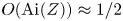 $O({\rm Ai}(Z)) \approx 1/2$ has been applied. Denoting
  $S = \sqrt {gh}\,t$ as the distance that the front of the trailing wave has travelled at time
  $t$, the equation above can be simplified as
 \begin{equation} \frac{O(\eta_{p})}{O(\eta_{+})} =O\left (-\frac{P_a^{c} h}{M_0}\left (2^{5}\,\frac{S}{h} \right)^{1/3} (Fr + 1)^{{-}1} \right ). \end{equation}
The influence of the free waves diminishes as the atmospheric pressure wave propagates to infinity, i.e.  $S \rightarrow \infty$. For the free wave amplitude to be the same order of magnitude as the leading wave,
  $O(\eta _{p})/O(\eta _{+}) = O(1)$, the travelling distance of the free wave must be within the relative distance
 \begin{equation} \frac{S}{h} < \frac{1}{2^{5}}\left (\frac{M_0}{P_a^{c} h}\right)^{3}(Fr +1 )^{3}. \end{equation}
These points will be illustrated further in § 4 with DART data captured during the 2022 Tonga event.
2.2. Shallow-water wave solutions
When the horizontal length scale of the atmospheric pressure wave is very long in comparison with the water depth, the generated water waves are non-dispersive long waves. The simplified solutions can be deduced readily from (2.11) by setting  $C \rightarrow \sqrt {gh}$. Thus the free surface shallow-water wave solutions can be expressed as
 \begin{equation}
\left.\begin{gathered} \eta =\eta_p +\eta_+ +
\eta_-, \\
\eta_p = \frac{1}{\rho g}\,\frac{1}{Fr^{2}
-1}\,P_a(x-C_pt), \\
\eta_+ = -\frac{1}{\rho
g}\,\frac{1}{2(Fr-1)}\,P_a(x-\sqrt{gh}\,t), \\
\eta_- = \frac{1}{\rho
g}\,\frac{1}{2(Fr+1)}\,P_a(x+\sqrt{gh}\,t).
\end{gathered}\right\}\end{equation}
\begin{equation}
\left.\begin{gathered} \eta =\eta_p +\eta_+ +
\eta_-, \\
\eta_p = \frac{1}{\rho g}\,\frac{1}{Fr^{2}
-1}\,P_a(x-C_pt), \\
\eta_+ = -\frac{1}{\rho
g}\,\frac{1}{2(Fr-1)}\,P_a(x-\sqrt{gh}\,t), \\
\eta_- = \frac{1}{\rho
g}\,\frac{1}{2(Fr+1)}\,P_a(x+\sqrt{gh}\,t).
\end{gathered}\right\}\end{equation}The solutions above, which can also be found in Pelinovsky et al. (Reference Pelinovsky, Talipova, Kurkin and Kharif2001) and Vennell (Reference Vennell2007), satisfy the linear shallow-water wave equations
 \begin{equation} \frac{\partial^{2} \eta}{\partial t^{2}} - gh\,\frac{\partial^{2} \eta}{\partial x^{2}} = \frac{gh}{\rho g}\,\frac{\partial^{2} P_a}{\partial x^{2}}, \end{equation}
with the assumption that wave motions start from the quiescent condition. Note that similar solutions for waves generated by moving pressure in a narrow channel (Dogan et al. Reference Dogan, Pelinovsky, Zaytsev, Metin, Tarakcioglu, Yalciner, Yalciner and Didenkulova2021) and moving obstacles (e.g. landslide, ship) have also been obtained (Tinti, Bortolucci & Chiavettieri Reference Tinti, Bortolucci and Chiavettieri2001; Lo Reference Lo2021). In addition, Vennell (Reference Vennell2007) studied the effect of bathymetric variations.
The corresponding horizontal velocity field can be expressed as
 \begin{equation}
\left.\begin{gathered} u =u_p +u_+ + u_-, \\
u_p ={-} \frac{1}{\rho C}\,\frac{Fr}{Fr^{2} -1}\,P_a(x-C_pt), \\
u_+ = -\frac{1}{\rho C}\,\frac{1}{2(Fr-1)}\,P_a(x-\sqrt{gh}\,t), \\
u_- = \frac{1}{\rho C}\,\frac{1}{2(Fr+1)}\,P_a(x+\sqrt{gh}\,t).
\end{gathered}\right\}\end{equation}
\begin{equation}
\left.\begin{gathered} u =u_p +u_+ + u_-, \\
u_p ={-} \frac{1}{\rho C}\,\frac{Fr}{Fr^{2} -1}\,P_a(x-C_pt), \\
u_+ = -\frac{1}{\rho C}\,\frac{1}{2(Fr-1)}\,P_a(x-\sqrt{gh}\,t), \\
u_- = \frac{1}{\rho C}\,\frac{1}{2(Fr+1)}\,P_a(x+\sqrt{gh}\,t).
\end{gathered}\right\}\end{equation} Lacking the frequency dispersion, the resulting wave patterns are much simpler and are easier to interpret. Moreover, most of the descriptions provided in § 2.1.1 remain valid, as captured in figure 1 (note that the horizontal axis represents  $Fr$ in this case). The ratio between the free wave and the locked wave can now be calculated as
 \begin{equation} O\left (\frac{\eta_p}{\eta_+}\right) = \frac{-2}{Fr + 1}. \end{equation}
For the subcritical condition ( $Fr < 1$), the locked wave is always larger than the free wave, up to a factor of 2 when
  $Fr \rightarrow 0$; for the supercritical condition (
 $Fr > 1$), the free wave becomes larger than the locked wave.
2.2.1. Comparison between dispersive and shallow-water solutions
The importance of the frequency dispersive effects is accumulative in time and space, and can be assessed by evaluating the ‘dispersion parameter’  $\tau$ (Glimsdal et al. Reference Glimsdal, Pedersen, Harbitz and Løvholt2013):
 \begin{equation} \tau = \frac{6 h^{2} D}{L^{3}}, \end{equation}
where  $L$ denotes the characteristic wavelength,
  $D$ represents the propagation distance, and
  $h$ is the water depth. Typically, if
  $\tau < 0.01$, then the frequency dispersion effects are negligible, whereas they are significant if
  $\tau > 0.1$. Consider the Tonga event (more details will be discussed in § 4): the typical water depth in the Pacific Ocean is
  $h = 4$ km, and the characteristic wavelength is
  $L = 800$ km. The dispersion parameter becomes
  $\tau = 0.002$ after the waves have travelled a distance 10 000 km. Therefore, the dispersion effects can be considered insignificant in the Pacific Ocean during the Tonga event. For dispersion effects to be significant (e.g.
  $\tau = 0.2$) under the same conditions, the propagation distance must be
  $D = 1.07 \times 10^{6}\ \textrm {km} \approx 1350 L$.
To portray the differences between the dispersive and non-dispersive solutions, we will apply (2.11) and (2.19) to an atmospheric pressure disturbance with the soliton shape,
 \begin{equation} P(x,t) = P_0 \operatorname{sech}^{2}[K(x - C_p t)], \end{equation}
in which  $P_0$ is the amplitude of pressure,
  $K = 2{\rm \pi} /L$ is the wave number, and
  $C_p$ is the fixed pressure wave celerity. This simple wave shape is convenient because its Fourier transform has an analytical expression:
 \begin{equation} \hat{P}(k) = \frac{k {\rm \pi}}{K^{2}}\,P_0 \operatorname{csch} \left[\frac{k {\rm \pi}}{2 K}\right]. \end{equation}
Yet calculating (2.11) requires a numerical integration procedure.
The values selected for the first test case are  $P_0 = 100$ hPa – which would translate into approximately 1 m free surface difference under static conditions –
  $C_p = 319\ \textrm {m}\ \textrm {s}^{-1}$,
  $L = 800$ km and
  $h = 4$ km, which are representative of the Tonga event. Under these conditions,
  $Fr = 1.61$. Figure 2 presents the comparison of the dispersive (2.11) and non-dispersive (2.19) solutions at different instants. Figure 2(a) presents the instant at which the trailing free waves have travelled 10 000 km, which is approximately the longest distance that the tsunami wave can travel from Tonga. According to the previous analysis based on Glimsdal et al. (Reference Glimsdal, Pedersen, Harbitz and Løvholt2013),
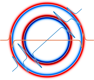
  $\tau = 0.002$, no significant dispersive effects are expected, and the results confirm that both solutions are virtually identical, both in the general overview and in the individual plots below it (which zoom in to each component). In addition, this validates that the shallow-water assumption is applicable for the given conditions. Figure 2(b) shows an extreme case in which the trailing waves have propagated over 1500 wavelengths, and have accumulated significant dispersive effects according to the previous analysis. Both free waves clearly show that the dispersive effects (blue line solution, (2.11)), with fast-decaying oscillating waves, are observed trailing the first wave, which is lower in height but longer than the shallow-water solution (red line). The ‘far-field’ approximation (yellow line) solution for the trailing free wave (
 $\eta _{+}$) presents a high resemblance with the fully dispersive solution, although the former presents a significant larger height. These differences can be attributed to the approximations inherent in (2.13) and the distance travelled, which may still not be large enough. The leading locked wave, however, does not show any differences between the three (dispersive, non-dispersive and ‘far-field’ approximation) solutions. Since this wave is forced by the pressure wave, this means that the leading wave propagates with a permanent shape and is effectively in the shallow-water regime.

Figure 2. Comparison between the dispersive ((2.11), in blue), non-dispersive ((2.19), in red) and ‘far-field’ approximation ((2.12) and (2.13), in yellow, bottom plots only) solutions at different instants. The pressure distribution is represented by a black line. Parameters:  $P_0 = 100$ hPa,
  $C_p = 319\ \textrm {m}\ \textrm {s}^{-1}$,
  $L = 800$ km and
  $h = 4$ km.
An additional case in which the pressure wave is much shorter ( $L = 1$ km) and the rest of parameters from the previous case are the same is shown in figure 3. The short wavelength,
  $h/L = 4$, means that these waves are in the deep-water regime. Therefore, the non-dispersive solution is not applicable, although it will be presented to enable a more direct comparison. Two snapshots are presented, when the free wave has propagated for 2 and 12.5 wavelengths (2 km and 12.5 km). In both cases
  $\tau \gtrapprox 200$, which means that dispersive effects are several orders of magnitude more important than in the previous case. Regarding the dispersive solution, the amplitude of the leading wave is significantly smaller, and the effective wavelength is longer, than the values for the non-dispersive solution. (The theoretical wavelength of a soliton is infinite. For convenience, the effective wavelength can be defined as the distance between those points at which the free surface elevation has reduced to a small fraction, e.g. 1 %, of the wave amplitude.) This is a direct result of (2.11), which, as discussed before, applies a scaling factor for each of the components. Since the pressure wave here is significantly shorter than before, each of these components will propagate at a much smaller celerity than long-wave celerity (
 $\sqrt {g h}$). Therefore, the effective amplification factor is also smaller, because
  $C_p$ remains constant. The free waves at both sides are way behind the non-dispersive solution due to the slower wave celerity. Dispersive effects can be noticed best in figure 3(b), presenting oscillations that are similar to those observed for the previous case.


These results point out that the dispersive solution is important when dealing with cases in which the pressure wave is not a long wave, or when waves propagate over a significant distance.
3. 2DH axisymmetric shallow-water wave problem
In the Tonga event, the atmospheric pressure is nearly axisymmetric and decays in the radial direction (Amores et al. Reference Amores, Montserrat, Marcos, Argüeso, Villalonga, Jordà and Gomis2022; Lynett et al. Reference Lynett2022). In this section, approximate solutions are sought for axisymmetric shallow-water waves being forced by an atmospheric pressure field. Thus in terms of the free surface elevation  $\eta (r,t)$, the governing equation is well-known:
 \begin{equation} \frac{\partial^{2} \eta}{\partial t^{2}} - gh\, \frac{1}{r}\,\frac{\partial}{\partial r}\left( r\,\frac{\partial \eta}{\partial r} \right ) = \frac{h}{\rho}\, \frac{1}{r}\,\frac{\partial}{\partial r}\left( r\,\frac{\partial P_a}{\partial r} \right ), \end{equation}
which can be rewritten in the form
 \begin{equation} \frac{\partial^{2} \sqrt{r}\,\eta}{\partial t^{2}} - gh\left(\frac{\partial^{2} \sqrt{r}\,\eta}{\partial r^{2}} + \frac{\sqrt{r}\,\eta}{4r^{2}}\right) = \frac{h}{\rho}\left(\frac{\partial^{2} \sqrt{r}\,P_a}{\partial r^{2}} + \frac{\sqrt{r}\,P_a}{4r^{2}}\right). \end{equation}
Consider  $l$ as the characteristic length scale of the atmospheric pressure and the induced water wave. For large
  $r\gg l$, the second term, relative to the first term inside the brackets of the equation above, is
  $O (l/r)^{2} \ll 1$ and can be neglected, resulting in an approximate governing equation in the far field as
 \begin{equation} \frac{\partial^{2} \sqrt{r}\,\eta}{\partial t^{2}} - gh\left(\frac{\partial^{2} \sqrt{r}\,\eta}{\partial r^{2}}\right) = \frac{h}{\rho}\left(\frac{\partial^{2} \sqrt{r}\,P_a}{\partial r^{2}}\right) . \end{equation}
Assuming that the atmospheric pressure takes the form
 \begin{equation} P_a = \sqrt{\frac{r_0}{r}}\,P_0(r-C_pt), \end{equation}
where  $r_0$ is a constant defining the radial location at which
  $P_a = P_0(r_0-C_pt)$, the analytical solution for (3.3) can be obtained as
 \begin{equation} \eta =\frac{1}{\rho g}\,\frac{1}{Fr^{2}-1}\,\sqrt{\frac{{r_0}}{{r}}}\left [ P_0(r-C_pt) - P_0(r-\sqrt{gh}\,t) \right ]. \end{equation}
This result can also be obtained by summing up the wave components of the 1DH solutions presented in (2.19), and multiplying the resulting expression by the radial decay factor  $\sqrt { r_0/r}$, since
  $\eta _{-}$ also propagates in the
  $r$-direction (due to radial symmetry).
4. Applications to the 2022 Tonga event
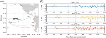
The theoretical far-field solutions are used to check the three DART station measurements (32 411, 32 401 and 32 404) during the Tonga event, shown in figure 4(a). The paths for the tsunamis reaching these stations are practically uninterrupted from the source. DART stations measure dynamic pressure at the bottom of the ocean. Normally, DART data are reported every 15 min; when the system detects a tsunami, the reported data resolution is improved to every 15 s. The reported data  $\zeta$ are calculated as follows (Rabinovich & Eblé Reference Rabinovich and Eblé2015):
 \begin{equation} \zeta = \eta + \frac{P_a}{\rho g}, \end{equation}
capturing both the atmospheric pressure disturbances and the induced water waves for the leading (locked) wave. These data need to be corrected to identify the actual water wave surface profile  $\eta$. For the Tonga event, the atmospheric pressure wave is long (
 $\sim$800 km) and propagates within the supercritical regime (
 $Fr \approx 1.5$) (Amores et al. Reference Amores, Montserrat, Marcos, Argüeso, Villalonga, Jordà and Gomis2022; Lynett et al. Reference Lynett2022). Thus the free surface elevation of the leading locked wave has the same sign and shape as the atmospheric pressure wave, and (2.19) can be used in (4.1) to find the following relationships:
 \begin{equation} P_a = \rho g \left( \frac{Fr^{2} - 1}{Fr^{2}} \right) \zeta \quad \text{and} \quad \eta = \frac{1}{Fr^{2}}\,\zeta. \end{equation}
This implies that the actual free surface elevation is smaller than the reported DART data, since  $Fr^{2} >1$. In addition, the first expression in (4.2a,b) provides a formula for estimating the magnitude of the atmospheric pressure at the DART station, using the reported
  $\zeta$. The time series shown in figure 4(b) contain both the reported DART data and the corrected data (black line) as per (4.2a,b).

Figure 4. (a) Geographical locations and (b) time series of free surface elevation reported by DART stations. The free surface elevations corrected by (4.2a,b) are in black lines. Grey arrows mark the arrival times of the leading locked waves and trailing free waves.
Practical information for the DART stations, such as the distance to Tonga and the average depth along the path, is listed in table 1. The arrival times for the leading and trailing waves are marked with grey arrows in figure 4(b) and listed along with the separation times (in the last column) in table 1. Based on the DART data at these stations, the Froude numbers range from 1.48 to 1.58, with average 1.54, confirming that the Tonga event is under the supercritical condition.
Table 1. Basic information from DART stations:  ${{S}}$ is great-circle distance from Tonga to the station in km;
  $\bar {{h}}$ is average depth along the path in m;
  ${t}_{{\eta }_{{p}}}$ and
  ${t}_{{\eta }_{{+}}}$ are arrival times of
  ${\eta }_{{p}}$ and
  ${\eta }_{{+}}$ in min;
  $\overline {{C}_{{p}}}$ and
  $\bar {{C}}$ are average celerities of
  ${\eta }_{{p}}$ and
  ${\eta }_{{+}}$ in
  $\textrm {km}\ \textrm {h}^{ -1}$;
  $\overline {Fr}$ is the average Froude number;
  ${A}_{{\eta }_{{p}}}$ and
  ${A'}_{{\eta }_{{p}}}$ are wave amplitudes of
  ${\eta }_{{p}}$ and their corrections (see (4.2a,b)) in cm;
  ${P}_{{\eta }_{{p}}}$ is the estimated peak pressure (see (4.2a,b)) in hPa;
  ${A}_{{\eta }_{{+}}}$ is the wave amplitude of
  ${\eta }_{{+}}$ in cm;
  ${\Delta t}_{{{theo}}}$ and
  ${\Delta t}_{{{obs}}}$ are time differences between the leading and trailing wave arrival times, from theoretical results and observations, in min.

During the event, the atmospheric pressure wave travels at the average velocity  $C_p \approx 1100\ \textrm {km}\ \textrm {h}^{-1}$ in the Pacific Ocean (Lynett et al. Reference Lynett2022), and the wave celerity of long water waves can be estimated as
  $C \approx 713\ \textrm {km}\ \textrm {h}^{-1}$, corresponding to average depth 4 km, representative of the Pacific Ocean. The theoretical time differences in the arrival times of the leading locked wave and the trailing free wave are listed in the second to last column in table 1. The differences between the theoretical and observed time lapses are below 10 % for DART stations 32 411 and 32 401. The difference for station 32 404 is larger, as the trailing (free) waves arrive 37 min faster than expected.
The observed and corrected amplitudes of the leading and trailing waves, and the estimated peak atmospheric pressure according to (4.2a,b), are also recorded in table 1. The peak pressures among these three DART stations range from 0.81 hPa to 1.28 hPa, with average 1.05 hPa, which is very close to 1.11 hPa, the value provided by the empirical model in Lynett et al. (Reference Lynett2022).
In table 2, the values of  $\eta _p/\eta +$ at each station are listed, including the reported and corrected DART data and various analytical solutions. The ratio is always negative for all cases, indicating that the leading and trailing waves have opposite sign. All the analytical solutions show that the amplitude ratios are close to 1, indicating that the shallow-water wave theory is adequate in describing this event. As expected, applying the correction (4.2a,b) reduces the amplitude of the leading locked wave, thus also decreases the value of the
  $\eta _p/\eta +$ ratio from average
  $-0.63$ to
  $-0.27$. These corrected values are significantly smaller than any of the analytical values. Nevertheless, the measured data and analytical solutions are in agreement in the order of magnitude. The differences between the measured data and theoretical solutions reflect the complexity of the problem, which includes effects of bathymetry, Earth's curvature and additional wave generation mechanisms related to the volcano explosion, which will travel together as part of the trailing wave package.
Table 2. Comparison of the  $\eta _p/\eta +$ ratio for the uncorrected (DART) and corrected (CDART) data, and the analytical solutions.

5. Concluding remarks
The analytical expressions developed herein cover dispersive and non-dispersive solutions, and can be applied to model water waves generated by atmospheric pressure disturbances travelling at supercritical and subcritical speeds. They provide significant insights into the resulting water wave characteristics, and can be used as benchmarks for numerical models. It is shown that the wave patterns generated under the supercritical condition are fundamentally different from those generated by a pressure disturbance propagating in a subcritical condition. Under the supercritical conditions, the atmospheric pressure disturbances induce a leading ‘locked’ wave with the same sign, i.e. a positive atmospheric pressure generates an elevated wave, which is counter-intuitive. Under the subcritical conditions, the locked wave is trailing and has opposite sign. Moreover, in the case in which the pressure wave is a long wave, the resulting water wave will have its same shape.
Atmospheric pressure disturbances also generate ‘free’ waves, whose sign and shape are also determined by the Froude number. These free waves are generated at the initial instant, and any other long waves produced during the explosion (e.g. mechanical blast, collapse of the caldera; Lynett et al. Reference Lynett2022) would also be travelling as part of the same wave package. Therefore, not all free waves that reach a location at the expected arrival time (based on the typical tsunami propagation celerity) are produced by the alternative mechanisms. In addition, locked waves are known to produce additional free waves due to scattering when they propagate over bathymetry changes (Vennell Reference Vennell2007). Thus any long waves arriving between the leading wave and pressure-driven trailing wave are likely to have been produced by this mechanism. Further study regarding the characteristics of these waves will be performed in a future paper.
We would also like to remark the importance of the dispersive effects when the pressure wave is short, relative to water depth, and/or if the waves propagate over a significant distance. In such cases, the frequency dispersive expressions provide the most accurate solution. Therefore, the dispersive solutions are required to generalize the problem of waves generated by pressure disturbances to account for potentially smaller eruptions or explosions.
Probably the most important conclusion of this work is that bottom-mounted pressure gauge measurements related to the locked waves need to be corrected to account for the additional pressure variations caused by the atmospheric pressure disturbances, which can be especially significant in the near field of the volcano explosion. The correction method presented in (4.2a,b) is novel, simple and useful in instances when simultaneous and co-located atmospheric pressure measurements to the DART system (or any pressure-based free surface elevation gauge) are not available.
In short, the analytical theories presented in this paper can explain the positive leading wave observed during Tonga's event, which is locked to the atmospheric pressure wave and thus arrives faster than expected based on the long-wave celerity.
Acknowledgements
P.L.-F.L. would like to acknowledge a National University of Singapore research grant (NRF2018NRF-NSFC003ES-002). This research was also supported in part by the Yushan Programme, Ministry of Education in Taiwan.
Declaration of interests
The authors report no conflict of interest.


 Open access