

1. Introduction
On a calving tidewater glacier, the position of the ice front is determined by a balance between the ice speed and the calving rate at the terminus.(Herein, and in most discussions of glacier calving, calving rate includes all processes by which ice is removed from a calving face, including calving of fragments ranging in size from individual crystals to icebergs the size of a building, as well as submarine melting.) For a terminus position to remain roughly constant, these two speeds must obviously be nearly equal. If that equality is not satisfied at a given time, then the terminus position will move until changed conditions of water depth against the calving face, valley geometry and mass input re-establish a balance.
Of the two rates that control a glacier’s position, only ice speed is reasonably well understood, physically and mathematically: given a geometry, reasonable assumptions about flow-law parameters and basal shear stress can provide suffcient information to estimate flow speeds from a numerical calculation. No such direct, physical calculation can be done for the calving rate, perhaps owing to the variety of scales and types of processes involved. A fundamental tenet of the above calculation is that glaciers that are thicker at the calving face move faster. Furthermore, glaciers that are thicker at the calving face end in deeper water because the subaerial part of a calving face is of relatively uniform height. Thus, if we consider a population consisting of a number of tidewater glaciers. with stable terminus positions, the thicker ones must have higher calving rates. The empirical relationship of calving speed to water depth at the calving face found by Reference Brown, Meier and PostBrown and others (1982) is an example of such a monotonic relationship between water depth and calving speed, and it has been applied with some success in a predictive manner on Columbia Glacier, Alaska, U.S.A. (Reference MeierMeier,1997).
In an earlier paper (Reference Hanson and HookeHanson and Hooke 2000, hereinafter referred to as HH), we presented a model of stresses and flow fields near the face of a grounded, tidewater calving glacier. In that paper, we investigated the stress field near and at a vertical calving face under various assumptions about the shape of the glacier surface profile and the basal stress conditions. One fundamental result was that the highest horizontal speeds at the calving face were in a zone extending from slightly above to just below the waterline. This created a tendency for the ice at the waterline to project out over the ice beneath the water, a result that might have been anticipated from Reference Hughes, Ruddiman and WrightHughes (1987). A second result was that the rate of overhang development (or the difference between maximum speed near the waterline and sliding speed at the base) increased with increasing water depth. The longitudinal deviatoric stress near the bed just back from the calving face also increased with increasing water depth, possibly facilitating bottom crevassing. These effects were not presented as a prediction of calving rate, but rather as a triggering mechanism. Ice near the calving face was presumed to be sufficiently crevassed that the only additional condition needed for calving was a tilt or buckling, creating a larger impetus to fall into the water than to remain with the glacier. These results may provide a physically based mechanism for the calving-speed/water-depth relationship found by Reference Brown, Meier and PostBrown and others (1982).
A different paradigm for calving models uses a kinematic boundary condition to control the terminus position (Reference Van der VeenVan der Veen, 1996, Reference Van der Veen2002). Van der Veen’s model focuses on the minimum total glacier thickness needed to avoid flotation. In the modified form used by Reference Vieli, Funk and BlatterVieli and others (2001) to model terminus changes at Hansbreen on Spitsbergen, the model is controlled by
where ρ w and ρ i are densities of water and ice, h w is the water depth at the calving face, h 0min is the minimum allowable total thickness ofthe glacier at the calving face, and q is a small number (<1) that will vary from glacier to glacier but presumably be constant with time at a given glacier over some range of terminus positions. The calving rate, u c, in this method arises from the change in terminus position required to maintain the minimum thickness. Although the apparent dependence of calving rate on water depth is obscured in Equation (1), implementation of this model still produces a calving rate that varies linearly with water depth (Reference Vieli, Funk and BlatterVieli and others, 2001, fig. 9).
The change with time in position ofthe terminus of the glacier (or change in glacier length, L) is given by dL
in which u 0 is glacier speed at the terminus. Because u c cannot be measured directly, it is always obtained as a residual in Equation (2) after measuring dL/dt and u 0. Normally, dL/dt ≪ u 0, so u c and u 0 will appear to be well correlated. The flotation model proposed by Reference Van der VeenVan der Veen (1996) requires this correlation, and assumes that it is always valid. No direct, causal connection has been proposed between calving speed and flow speed. They may be mutually correlated via their common dependence on ice thickness and hence water depth, as well as via the necessity of ice movement to continually recreate the conditions needed for calving. The dependence of the patterns noted in HH upon water depth supports such a connection. Reference Van der VeenVan der Veen (2002) calls the correlation between calving speeds and height spurious, implying that they result from sampling and would vanish if sufficient data were collected. We disagree. Many quantities (speed, overhang rate, various stress components) increase with either glacier thickness or water depth (which are themselves strongly correlated), and to claim that these have no influence on calving rate is unfounded, given our lack of understanding of calving processes such as fracture initiation and propagation and submarine melt.
The results in HH were robust with respect to assumptions regarding basal sliding speed, surface profile, height of the subaerial calving face, lateral stress shape factor, presence or absence of crevasses, and ice rheology. All of these factors affected the rate of overhang development to a greater or lesser degree, and hence, presumably, could affect the calving speed, but none of them obscured the increase of overhang development with submarine calving-face height (for families of simulations in which thickness was varied while all other factors were held constant). Several other robust features that might affect calving were also noted in HH. The highest values of the longitudinal deviatoric stress, ![]() were near the waterline height a few tens of meters back from the calving face. Also, a small zone of compressive deviatoric longitudinal stress appeared at the surface of the glacier a short distance (30–40 m) back from the calving face.
were near the waterline height a few tens of meters back from the calving face. Also, a small zone of compressive deviatoric longitudinal stress appeared at the surface of the glacier a short distance (30–40 m) back from the calving face.
This paper further explores simulated stress fields near a calving face, expanding on HH by showing the influence of rheological parameters on both the surface compressive zone and the tendency of the calving face to bulge out near the waterline. Additionally, the effects of subaerial calvingface height variations are explored, whereas HH was primarily concerned with water-depth variations.
2. The Model
As in HH, the model used in this study is the vertical flowplane finite-element model described by Reference HansonHanson (1990). As used in these studies, the model solves steady conservation of momentum and incompressible conservation of mass:

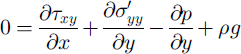

in which x is a horizontal coordinate and y is directed vertically upward, u and v are their corresponding velocity components, ![]() and
and ![]() are the corresponding deviatoric stresses from the diagonal of the stress tensor, τxy
= τyx
is the shear stress, g is acceleration of gravity, p is pressure and ρ is density (constant at 900 kg m−3 in all simulations). These equations are solved using a Reference GlenGlen (1955)-type power law,
are the corresponding deviatoric stresses from the diagonal of the stress tensor, τxy
= τyx
is the shear stress, g is acceleration of gravity, p is pressure and ρ is density (constant at 900 kg m−3 in all simulations). These equations are solved using a Reference GlenGlen (1955)-type power law,
where τ
ij
and ![]() are any corresponding elements of the deviatoric-stress and strain-rate tensors, and
are any corresponding elements of the deviatoric-stress and strain-rate tensors, and ![]() is the effective strain rate,
is the effective strain rate, ![]() . All of these simulations were carried out with constant B = 200 kPa a1/n
, and most were carried out with a constant enhancement factor, E = 1 except as discussed in section 3.2 on near-surface softening. The flow-law exponent, n, was a constant within any given simulation, and n = 3 was used in all simulations except those where variation of n between simulations is specifically discussed. The equations are solved using Galerkin’s method on linear quadrilateral elements, in which the non-linear rheologies (n ≠ 1) require iteration.
. All of these simulations were carried out with constant B = 200 kPa a1/n
, and most were carried out with a constant enhancement factor, E = 1 except as discussed in section 3.2 on near-surface softening. The flow-law exponent, n, was a constant within any given simulation, and n = 3 was used in all simulations except those where variation of n between simulations is specifically discussed. The equations are solved using Galerkin’s method on linear quadrilateral elements, in which the non-linear rheologies (n ≠ 1) require iteration.
The finite-element grids for tidewater calving glaciers consisted of elements in columns 5 m wide everywhere, with element heights of 5 m at the calving face. The element height increased back from the calving face in order to span the increasing glacier thickness with a constant number of elements. All of the grids for these experiments had perfectly flat bottoms and a simulated length up-ice from the calving face of 2000 m.(The coordinate system and some of the notation are illustrated in Figure 1a.) The origin of the coordinate system is always the bottom of the glacier terminus. In these and some later contour diagrams, a horizontal axis is labeled as −x, which is equivalent to “distance from calving face”. Use of the negative coordinate within the model preserved the usual sense of x increasing left-to-right and positive horizontal velocity, while allowing the convenience of x = 0 at the calving face. Only the section within a few hundred meters ofthe calving face was analyzed; the remainder of the simulation was primarily intended to buffer the calving face from effects of the up-ice boundary conditions.

Fig. 1. Contour diagrams of simulated fields for a run in which total height of the calving face, h
0, is 200 m, water depth, h
w, is 140 m, and surface softening was not used, E
max = 1. Arrows and notations in (a) point out features that are tabulated for this and other simulations. Speeds are in m a−1, stresses in kPa. Gray bars indicate the water level against the calving face. (a) Horizontal speed, u. (b) Vertical speed, v (downward velocities plotted positive here). (c) Deviatoric longitudinal stress, ![]() ; contours dashed when negative. (d) Shear stress, τ
xy. The sense of shear implied by differing signs of τ
xy is schematically illustrated by diagrams showing the approximate deformation with time of an initially square piece of the flowplane.
; contours dashed when negative. (d) Shear stress, τ
xy. The sense of shear implied by differing signs of τ
xy is schematically illustrated by diagrams showing the approximate deformation with time of an initially square piece of the flowplane.
The base of the simulated glacier tongue was subjected to a mixed boundary condition of velocity and stress. At each basal node, the vertical component of velocity was set to zero. Horizontal velocity components at these nodes were not fixed to particular values by boundary conditions, but were subjected to a resistive stress. The amount of resistive stress applied in a given simulation varied with the thickness at the calving face in that simulation. Basal shear stress τ b was assumed to increase with margin thickness according to a linear relation discussed in HH, τ b = a + bh 0, where a = 81 kPa and b = 0:668 kPa m−1. That relationwasbased on a force-balance analysis of glaciers used by Reference Brown, Meier and PostBrown and others (1982). When applied to glaciers with front thicknesses, h 0, of 100–300 m, this produces basal resistive stresses of 147–281 kPa, with a value of 214 kPa at h 0 = 200 m. These were applied uniformly as resistive stresses (horizontal stresses against the direction of flow) along the entire base of the glacier.
Other boundary conditions included a horizontal inflow of ∼1000 m a−1 at the up-glacier end of the simulated domain and a water pressure applied to the submerged portion of the calving face. The velocity at the up-ice boundary increased slightly with height, following the plane-strain solution of Reference NyeNye (1957). As in HH, the inflow boundary conditions turn out to be entirely irrelevant in producing the stress and deformation fields near the glacier margin. The subaerial portion of the calving face and the upper surface of the glacier were free surfaces, mathematically equivalent to an applied stress boundary condition of zero magnitude.
3. Effects of Rheology on Near-Surface Stress Patterns
3.1. Control run
As a basis for comparison with other simulations, we made a control run with a glacier thickness of 200 m in water 140 m deep. Following the procedure described in HH, this glacier had a parabolic surface profile that provided a constant driving stress τ
d = ρgh(x) α(x) = 214 kPa, where α(x) and h(x) represent the slope and height along the surface (Fig. 1a). The value of 214 kPa comes from the linear relationship described above. Fields of horizontal velocity, u, vertical velocity, v, shear stress, τxy
, and deviatoric longitudinal stress, ![]() , for this control run are presented in Figure 1. (These are pure flowplane simulations with no parameterized lateral strains, so
, for this control run are presented in Figure 1. (These are pure flowplane simulations with no parameterized lateral strains, so ![]() ) The difference from model runs in HH is primarily in the use of a unit lateral-stress shape factor.
) The difference from model runs in HH is primarily in the use of a unit lateral-stress shape factor.
Near the calving face, the horizontal speed and longitudinal strain rates are highest in a zone extending from slightly above to somewhat below the waterline, with highest strain rates 30–60 m up-ice from, and highest speeds directly at, the calving face (Fig. 1). This zone of maximum velocity represents a form of extrusion flow, inasmuch as the velocity increases from the top of the calving face to slightly below the waterline (see the shear diagrams in Figure 1d for the sense of the deformation). All of these simulations show a maximum in τxy just above the waterline, where the extrusional deformation is strongest.
A puzzling result, clearly present in this control run and in all simulations discussed in HH, is a small area of compressive deviatoric longitudinal stress at the surface near the calving face that is barely visible in Figure 1c. With the model formulation used here, the sign of the longitudinal deviatoric stresses always matches the sign of the corresponding strain-rate tensor component, so compressive motion is implied. The higher horizontal speeds and longitudinal strain rates at the waterline require, via conservation of mass, a considerable downward vertical velocity in the area 50–100 m up-ice from the calving face. The compressional zone at the top near the calving face usually extends from about 20 m to about 60 m back from the face, and normally encompasses only the uppermost ∼5 m thick layer of elements.
Situations such as that above, in which velocity increases with depth, can only occur under special circumstances, and a vertical wall of ice unsupported by either water or ice certainly constitutes such a special circumstance. Simply put, the unsupported wall tends to buckle outward rather than tip over. This buckling was first noticed during early development of the finite-element model described by Reference Hooke, Raymond, Hotchkiss and GustafsonHooke and others (1979), which was a precursor to the model used in the present paper. In those earlier simulations, a rectangular column of ice, unsupported except at the base, would bulge out near the base while sinking more rapidly in the center than at the outer edges. Similar simulations using the current finite-element model show that this buckling occurs whether the column is frozen to the bed or freely sliding (Fig. 2). The effect is extreme enough that the uppermost velocity vectors take a very slight backwards direction (not visible at the scale of Figure 2). The components of the largest vectors at the top of Figure 2 are roughly v = 6 m a−1 and u = −0:3 m a−1. In these column simulations, the element size was reduced to 2 m squares, so the compressive zone goes deeper than a single layer of elements.

Fig. 2. Velocity vectors (arrows) and ![]() fields (contours in k Pa) for simulations of a 40 m tall vertical column of ice that is unsupported on the right side, using 2 m square elements. Left sides are fixed at zero horizontal velocity as if this were the right half of a symmetric, 40 m wide column. Heavy dotted lines indicate the shape each column would have were it allowed to deform at these velocities for one half-year. Velocity vectors are shown at every other node in each dimension. (a) Basal velocity fixed at zero. (b) Basal horizontal velocity free to slide, with no applied shear resistance.
fields (contours in k Pa) for simulations of a 40 m tall vertical column of ice that is unsupported on the right side, using 2 m square elements. Left sides are fixed at zero horizontal velocity as if this were the right half of a symmetric, 40 m wide column. Heavy dotted lines indicate the shape each column would have were it allowed to deform at these velocities for one half-year. Velocity vectors are shown at every other node in each dimension. (a) Basal velocity fixed at zero. (b) Basal horizontal velocity free to slide, with no applied shear resistance.
The compressive zone was present in all simulations calculated for HH. This compressive zone is not removed by any surface-profile or basal shear-stress assumption that we have tried. Nor is it removed by including modest departures from the purely vertical calving face. A variety of simulations, mostly using the control run heights (h 0 = 200m, h c = 60m), tested non-vertical terminus faces. Simulations in which the subaerial calving face sloped backwards linearly from the waterline so that the top position was as much as 20 m back from the waterline did not remove it, nor did less physically justifiable simulations in which the subaerial calving face leaned outward above the waterline. Departures from vertical of the face below the waterline, whether of an overhanging calving face or of an extending submarine toe, have very little effect on the finite-element solution above the waterline.
This compressive zone provides a distinct contrast with perceived reality. Although we lack measurements of surface strain-rate fields near a calving face, our qualitative observations and many pictures in Reference Post and LaChapellePost and LaChapelle (2000) indicate that tidewater calving glaciers are usually heavily crevassed near their margins. This would seem to be incompatible with compression. However, the compression rates (negative longitudinal strain rates) obtained in our simulations would not necessarily show up in aerial photography. In nature, crevasses form well up-glacier from the location, in our models, of the zone of compression. In order-of-magnitude terms: a compression rate of 0.1 a−1 (based on our simulations) acting over a distance of tens of meters on a glacier that is moving at speeds of meters per day will only close a large crevasse by a few centimeters before the crevasse becomes (temporarily) the calving face, en route to becoming an iceberg face. Thus, while we have no evidence that such a compressive zone exists in any real calving tidewater glaciers, images of heavily crevassed glacier surfaces do not rule out the possibility. However, further simulations modifying the rheology of the ice have shown that it is possible to remove the compressive zone.
3.2. Surface softening
A finite-element model, used properly, calculates numerically accurate solutions to the mathematical principles that we think describe glacier motion. The numerical scheme and its computer-program implementation used here have been sufficiently tested in previous studies to ensure that this is the case for this program. Three mathematically expressed principles are used in creating the model: a steady, viscous force balance (Equations (3) and (4)), conservation of mass for an incompressible fluid (Equation (5)) and the Reference GlenGlen (1955) power law for flow with constant B and n (Equation (6)).
Incompressibility on the large scale may be too strong an assumption for a heavily crevassed glacier surface. While it would be very easy to specify a smaller in the top few layers of elements, doing so only adds another variable that must be interpreted, and minor reductions in density have no significant effect on the results shown. Movement deep in the ice controls the surface motion, and removing a few tons of ice from the empty crevasses has only a minor effect on the dynamics of the deeper ice. A more tractable departure from our fundamental principles is to modify the flow law in the upper layers of the glacier in response to the crevassing. Once again, we have no specific law to apply, but, on a sufficiently large scale (larger than the scale of seracs), ice will be softened by the presence of cracks and crevasses. This is not an actual softening of the ice; rather it reflects the fact that stress can be relieved by motions along pre-existing cracks more easily than in uncrevassed ice. This softening can be introduced into the model by means of an enhancement factor, E in Equation (6), such as is traditionally introduced to simulate the effects of preferred crystal orientation. Reducing the viscosity to simulate pervasive cracking may not be common for glacier modeling. However, in sea-ice modeling, a plastic rheology or other stress-limited rheology is commonly used to account for the fact that once cracking has been initiated, the ability of ice to sustain stress is severely reduced (e.g. Reference Sammonds, Rist, Dempsey, Shen and ShapiroSammonds and Rist, 2000).
In the surface-softened simulations used here, a certain enhancement factor is chosen for the topmost layer of elements. In layers below the top, the enhancement factor is reduced linearly until it is back to unity in the ninth element layer. Thus, the upper 40 m of ice are at least partially softened near the calving face, and the thickness of the softened layer increases slightly as element thicknesses increase back from the calving face. The pattern of softening was extended back from the calving face uniformly for 500 m.
A series of simulations using the same geometry as the control simulation (E
max = 1) were generated with values of E
max of 2, 5, 10 and 20, respectively (Table 1). Following through the 200 m thick simulations, as the softening increased, the maximum in ![]() (Table 1, column a) slightly below the waterline and up-ice from the calving face increases in magnitude, without significantly changing position (Table 1, column a). The region of compressive (negative)
(Table 1, column a) slightly below the waterline and up-ice from the calving face increases in magnitude, without significantly changing position (Table 1, column a). The region of compressive (negative) ![]() (Fig. 3; Table 1, column c) gets smaller with E
max = 2, becomes very small for E
max = 5, and becomes undetectable with higher softenings.
(Fig. 3; Table 1, column c) gets smaller with E
max = 2, becomes very small for E
max = 5, and becomes undetectable with higher softenings.

Fig. 3. Contour diagrams of ![]() for simulations in which the crevasse softening factor, E, varies. Softening increases linearly from E
max = 1 at 40 m depth to the given maximum E
max at the surface. All simulations were 200 m thick at the margin; only the top 100 m is shown. Gray bars indicate the level of water against the calving face. Contour interval is 20 k Pa. (a) E
max = 2; (b) E
max = 5; (c) E
max = 10; (d) E
max = 20. (Compare with Figure 1c for E
max = 1.)
for simulations in which the crevasse softening factor, E, varies. Softening increases linearly from E
max = 1 at 40 m depth to the given maximum E
max at the surface. All simulations were 200 m thick at the margin; only the top 100 m is shown. Gray bars indicate the level of water against the calving face. Contour interval is 20 k Pa. (a) E
max = 2; (b) E
max = 5; (c) E
max = 10; (d) E
max = 20. (Compare with Figure 1c for E
max = 1.)
Table 1. Summary of a series of model runs distinguished by their calving-face thicknesses h 0 and the maximum degree of surface softening E max. All positions in m, speeds in m a−1, stresses in k Pa

The value of ![]() must approach zero at the upper corner of the calving face. (Stress tensor components and pressures are calculated as constants within each element in this finite element formulation, so
must approach zero at the upper corner of the calving face. (Stress tensor components and pressures are calculated as constants within each element in this finite element formulation, so ![]() is not precisely zero in the upper corner element because that element is an almost square 5 m by 5 m region — small but not infinitesimal.) Once the softening is adequate to prevent the formation of a compressive zone (E
max ≥ 10), the pattern of
is not precisely zero in the upper corner element because that element is an almost square 5 m by 5 m region — small but not infinitesimal.) Once the softening is adequate to prevent the formation of a compressive zone (E
max ≥ 10), the pattern of ![]() near the surface becomes quite simple. Up-ice from a position 100 m or so back from the calving face, near-surface deviatoric longitudinal stresses have values nearly independent of x (contours become more parallel to the surface as softnesses increase in Figures 1c and 3). Moving upward in the first column of elements at the calving face,
near the surface becomes quite simple. Up-ice from a position 100 m or so back from the calving face, near-surface deviatoric longitudinal stresses have values nearly independent of x (contours become more parallel to the surface as softnesses increase in Figures 1c and 3). Moving upward in the first column of elements at the calving face, ![]() decreases monotonically and nearly linearly toward the corner element. The value of
decreases monotonically and nearly linearly toward the corner element. The value of ![]() in the upper part of the glacier decreases with increased softening (Table 1, column a), as should be expected, but this decrease is not nearly as great, proportionally, as the change in enhancement factor. However, as the softening increases, the position of the onset of softening at approximately 40 m depth becomes well delineated by a strong gradient in contours of
in the upper part of the glacier decreases with increased softening (Table 1, column a), as should be expected, but this decrease is not nearly as great, proportionally, as the change in enhancement factor. However, as the softening increases, the position of the onset of softening at approximately 40 m depth becomes well delineated by a strong gradient in contours of ![]() (Fig.3c and d in particular).
(Fig.3c and d in particular).
Shear stresses τxy also change as the softening increases. Consider the maximum shear stress maintained in the region of the glacier above the waterline. As softening increases, these shear stress maxima decrease in magnitude and move back from the calving face (Table 1, column b). While the shear stress (and implied slumping-out rotation) decreases with increased softening, it remains significant, so the tendency for the calving face to buckle outward at the waterline is not removed in these simulations.
A primary result of HH was that increasing submarine calving-face height (with a constant h c = 60 m) produced an increasing rate of overhang development near the waterline. Sets of runs at each of five terminus thicknesses (h 0 varying from 100 to 300 m in 50 m increments) were carried out with three different maximum E max values: 1, 5 and 10. For any given softening as the ice got thicker, both u max and v max generally got larger (Table 1, columns d and e). The fundamental results from HH are thus maintained at all softnesses.
The differences between the maximum speed at the calving face and the speeds at the top and base of the ice front serve as measures of the rate of overhang development. Let us define two departures Δu top = u max − u top and Δu base = u max − u base, where all u values are at the calving face (i.e. x = const = 0 and only y varies between the points considered). Looking at these departures (Table 1, columns f and g) the increase in overhang development with height indicated by the Δu base values is large at all softnesses, and the effect increases with increasing E max. The Δu top values show that buckling-out behavior is reduced with the softening, which again correlates well with the removal of the compressive zone.
3.3. Effects of varying the flow-law exponent
Our objective in this subsection is to explain the compressive zone at the surface. To focus on this zone, experiments were carried out with the column model described earlier. The bed was assumed to be frozen, as in the simulation shown in Figure 2a.
The pressure in the center of the column (left edge of panels in Fig. 4) increases with depth, roughly linearly as cryostatic pressure is the dominant effect. However, the pressure along the free face (rightedge of panels in Fig. 4) is atmospheric. Thus, the size of the horizontal pressure gradient from the center to the edge ofthe column increases (linearly) with depth and, as in any fluid, this results in an increase in u with depth along the free surface. This increase in u with depth is nearly linear in the upper part of the column, but close to the bed it is modified by basal drag.

Fig. 4. Contours of u, v, ![]() and τ
xy for simulations of a 40 m tall vertical column of ice (symmetric about the left side, as in Figure 2) using 2 m square elements. Each column presents fields from a different simulation, with the only variation between simulations being the value of the flow-law exponent, n. A no-slip basal boundary condition was used. The sense of shear of τ
xy is illustrated schematically with deforming squares, as in Figure 1d. (All vertical velocities, v, are downward but are plotted with positive, solid contours to clarify the graphs.)
and τ
xy for simulations of a 40 m tall vertical column of ice (symmetric about the left side, as in Figure 2) using 2 m square elements. Each column presents fields from a different simulation, with the only variation between simulations being the value of the flow-law exponent, n. A no-slip basal boundary condition was used. The sense of shear of τ
xy is illustrated schematically with deforming squares, as in Figure 1d. (All vertical velocities, v, are downward but are plotted with positive, solid contours to clarify the graphs.)
In a power-law fluid, the viscosity decreases as effective stress increases, whereas in a Newtonian fluid (n = 1) the viscosity is independent of stress. High stresses in these columns are concentrated near the bottom (third and fourth rows of Fig. 4). Therefore, lower viscosities will also be concentrated near the bottom of the columns for which n > 1, and the higher the value of n, the more the softening near the bottom.
However, the horizontal pressure-gradient field will be approximately the same in all cases, increasing linearly with depth. When this pressure-gradient field is applied to material that is softer on the bottom and stiffer on top, the greater response at the bottom causes a net counterclockwise rotation of the column. The changing sense of the deformation is visible in the changing slope of the vertical velocity contour lines near the bottom of each column (Fig. 4, second row). The downward flow in the Newtonian case (n = 1) is relatively even across the column, indicated by nearly horizontal contour lines. As n increases, the concentration of downward flow near the left side (symmetric axis) of the column (at the top of the column) increases, indicated by a higher slope of the contour lines of v. With this increased concentration of vertical flow near the symmetry axis, u near the surface becomes negative as ice falls backward into the area of maximum downward flow.
3.4. Discussion
In the previous subsections, the compressive zone near the top of the glacier could be removed by relative softening in two different ways: (1) direct viscous modification via enhancement factors, and (2) reducing the power-law exponent. The experiments with varying n show how this phenomenon can arise in ice. The softer bottom and stiffer upper ice in a power-law fluid provide a weak analogy to the pratfall of slipping on a banana peel (or on a glacier after a fresh rain) in which the feet slip out so rapidly that the head moves backwards.
As discussed above, we cannot rule out the possibility that such a compressive zone occurs in nature. However, emulating pervasive crevassing via direct modification of the viscosity removed the compressive zone near the surface, but did not change any of the other essential results of HH. Softening the near-surface ice is not a direct simulation of the effect of crevassing, of course. The softened ice has the mass and hence driving force of uncrevassed ice, and hence overstates the driving force. It is also less compressible than crevassed ice. As a result of these differences between model and reality, and the subtle character of the effects, we have no way of knowing whether the compressive zone should be expected in real tidewater calving glaciers. However, we believe we have shown: (1) that it is not a numerical artifice, and (2) that the presence or absence of such a compressive zone does not affect the basic conclusions of HH, and may actually enhance the development of the submarine overhang.
4. Effects of Subaerial Calving-Face Height
4.1. Subaerial calving faces above water
In all of the runs discussed in section 3, we used a subaerial calving-face height, h c, of 60 m. On the glaciers studied by Reference Brown, Meier and PostBrown and others (1982), h c ranged from 30 to 92 m with a mean of 61m; only 4 of their 17 glaciers had subaerial calving-face heights outside the range 48–70 m. Reference Brown, Meier and PostBrown and others (1982) could not find any statistical relation between calving speed and h c.
Because simulations in HH did not test the u c vs h c relationship, we report here a set of experiments designed to do that. The simulations with varying h c were carried out with two forms of variation: for a water depth, h w, of 100 m, h c was allowed to vary from 20 to 100 m, and for a constant total face height, h 0 = 200 m, h c was allowed to vary from 30 to 100 m (Fig. 5; see Fig. 1a for notation). Water levels were, in some cases, near, but never above, flotation level. (Simulations with water levels above flotation produce physically unreasonable results because the basal boundary conditions — vertical velocities specified at zero — do not allow the glacier to float. Our interest herein is in tidewater glaciers, not ice shelves, so this limitation is not a concern.) These runs were repeated with near-surface softening of E max = 1 and E max = 10. Softening did not affect the results discussed here, so only the E max = 10 results are shown because of the simpler stress pattern that results when the compression zone is removed.

Fig. 5. Variation of velocity and stress indices with subaerial calving-face height, h
c (vertical axis). Points are labeled with values of total height at margin, h
0, commonly with two points being visually indistinguishable. (a) Speeds, including Δu
max, Δu
base and Δu
top. Values <1 m a−1are omitted. (b) Maximum stresses, including ![]() and τ
xy.
and τ
xy.
In these simulations, all of the following increase with subaerial calving-face height, h
c: the maximum speed at the calving face, u
max; the slumping-out rate, Δu
top; the overhang rate, Δu
base; ![]() at the maximum behind the waterline; and τxy
at the maximum behind the waterline (Fig. 5). Of these parameters, only Δu
base varies appreciably with h
w, as shown by the fact that the points for a given h
c but with different h
0 are indistinguishable, or almost so, in the other curves in Figure 5.
at the maximum behind the waterline; and τxy
at the maximum behind the waterline (Fig. 5). Of these parameters, only Δu
base varies appreciably with h
w, as shown by the fact that the points for a given h
c but with different h
0 are indistinguishable, or almost so, in the other curves in Figure 5.
We cannot calculate calving speed, u c, directly with the finite-element model because this model does not simulate failure. However, if we are correct in relating u c to Δu base as in HH, the increase in Δu base with h c suggests that u c should be positively correlated with h c. This effect is more pronounced for the situation in which h c increases with h 0 held constant (i.e. in the left branch of the curves for Δu base in Figure 5, water depth, h w is constant at 100 m so the slope of the curve indicates a positive relationship between h c and Δu base). Reference Brown, Meier and PostBrown and others (1982) may not have found this correlation owing to the limited range of h c in their dataset and the influence of other factors.
The change in ![]() with h
c (Fig. 5b) may indicate that h
c has an important role as a limiting factor. The tensile stress necessary to induce crevassing in a real glacier is not known, but Reference IkenIken (1978) used 100 kPa as a rule of thumb for onset of crevassing, and similar numbers have been used as yield stress in plastic-flow models (Reference PatersonPaterson,1994). While the tensile strength of pure ice can be three times to more than ten times higher than this (Reference Higashi, Riehl, Bullemer and EngelhardtHigashi,1969; Reference HobbsHobbs,1975), Reference KeneallyKeneally (2003) found that a tensile stress of 100 kPa produced crevasses of reasonable depths (∼30 m) whereas 250 kPa produced maximum crevasse depths of >70 m in a theoretical calculation involving plastic deformation. Within this model, longitudinal deviatoric stresses are used rather than full tensile stresses, but these are near the surface of the ice. We see that with h
c of 20 m, near-surface values of
with h
c (Fig. 5b) may indicate that h
c has an important role as a limiting factor. The tensile stress necessary to induce crevassing in a real glacier is not known, but Reference IkenIken (1978) used 100 kPa as a rule of thumb for onset of crevassing, and similar numbers have been used as yield stress in plastic-flow models (Reference PatersonPaterson,1994). While the tensile strength of pure ice can be three times to more than ten times higher than this (Reference Higashi, Riehl, Bullemer and EngelhardtHigashi,1969; Reference HobbsHobbs,1975), Reference KeneallyKeneally (2003) found that a tensile stress of 100 kPa produced crevasses of reasonable depths (∼30 m) whereas 250 kPa produced maximum crevasse depths of >70 m in a theoretical calculation involving plastic deformation. Within this model, longitudinal deviatoric stresses are used rather than full tensile stresses, but these are near the surface of the ice. We see that with h
c of 20 m, near-surface values of ![]() are around 40 kPa, and
are around 40 kPa, and ![]() reaches 96 kPa only at a the local maximum (see Fig. 1c for an example of the spatial variation in
reaches 96 kPa only at a the local maximum (see Fig. 1c for an example of the spatial variation in ![]() ) . General (as opposed to maximum) near-surface longitudinal stress deviators do not approach 100 kPa until h
c is about 60 m.
) . General (as opposed to maximum) near-surface longitudinal stress deviators do not approach 100 kPa until h
c is about 60 m.
These simulations raise the possibility that calving rates are indeed influenced by h
c in a way that the Reference Brown, Meier and PostBrown and others (1982) dataset cannot show. Simply put, a glacier with a low calving face, h
c
< 40 m or so, would be less susceptible to deep crevassing and would have a low calving rate. A glacier with h
c near the high end of these simulations, approaching 100 m, has very high ![]() and would presumably be very weak. Higher h
c also leads to a rapidly increasing slumping rate, Δu
top (note the concave upward shape of the Δu
top graph and logarithmic abscissa in Figure 5a). A potential implication that subaerial calving-face heights are limited in both minimum and maximum height by
and would presumably be very weak. Higher h
c also leads to a rapidly increasing slumping rate, Δu
top (note the concave upward shape of the Δu
top graph and logarithmic abscissa in Figure 5a). A potential implication that subaerial calving-face heights are limited in both minimum and maximum height by ![]() is explored further in section 4.2.
is explored further in section 4.2.
4.2. Subaerial calving faces without water
As an additional check on this result, simulations were performed on glaciers with vertical faces that do not terminate in water. These simulations were partly inspired by Antarctic dry-valley glaciers, which in some cases have vertical calving faces from which bergs spall off without apparent buckling (personal communication from B. Hallet, 1999). These glaciers are frozen to their beds (temperatures everywhere below −20°C) and are much thinner and slower (Reference ChinnChinn, 1988) than the tidewater glaciers that have been the topic so far.
For these simulations, element thicknesses were reduced to 2 m to accommodate the much smaller overall thickness of the glaciers. The driving-stress/thickness relation derived in HH cannot be expected to hold under these circumstances, so the surface slope at and just up-glacier from the calving face was set at 0.05, and a parabolic surface profile was calculated to hold driving stress constant. The temperature-dependent viscosity factor B was set to 575 kPa a1/n , consistent with a constant temperature of −20°C and the equation for B given in Reference HookeHooke (1981). Glacier thickness in these simulations ranged from 20 to 100 m (Table 2 upper group; Fig. 6).

Fig. 6. Variation of velocity and stress indices with face height for water-free, zero basal velocity simulations listed in Table 2. (a) Speeds, including u
max and Δu
top along with the height at which u
max occurs on the face, read against the upper axis. (b) Maximum values of ![]() and τxy
in the flowplane.
and τxy
in the flowplane.
Table 2. Summary of a series of model runs with no water at the face, distinguished by face heights, h 0. All positions in m, speeds in m a−1, stresses in kPa

A second set of waterless glacier simulations was performed in which the glacier was allowed to slide freely with an applied basal stress equal to the driving stress (Table 2 lower group). These produce substantially higher speeds than the simulations in which the ice is frozen to the bed, but the nature of the variation with height is the same, including the increase in bulging rate with thickness.
As with conventional tidewater glaciers, these simulations produce bulging in the lower part of the (subaerial) face. However, the bulging rate (Δu top) is negligible for the thinnest glaciers, so the toppling character of calving events on dry-valley glaciers is reasonable. In these simulations, the tendency of the glacier to produce a bulge low in the calving face is demonstrated at all thicknesses, with a maximum velocity at about a quarter of the total height (the y(u max) curve in Fig. 6).
From these waterless simulations, we learn that: (1) the results of section 4.1 regarding variation of h
c are not unique to glaciers that terminate in water, and (2) the “slumping” results of the column-model simulations illustrated in Figures 2 and 4 are not unique to a collapsing column with insignificant horizontal extent. For a low value of h
c = h
0 in the waterless simulations, say 20–40 m, the character of the velocity field near the margin is mostly established only within a few tens of meters of the margin (Fig. 7). These simulations also show that the increase of ![]() with h
c (Table 2; Fig. 6b) does not depend dramatically on either the presence of water or the presence of an underlying sliding or deformation speed beneath the ice cliff (compare
with h
c (Table 2; Fig. 6b) does not depend dramatically on either the presence of water or the presence of an underlying sliding or deformation speed beneath the ice cliff (compare ![]() values in Figures 5b and 6b, also visible in Figure 7). Simulations herein show that the majority calving faces in Reference Brown, Meier and PostBrown and others (1982) have h
c values in the range for which
values in Figures 5b and 6b, also visible in Figure 7). Simulations herein show that the majority calving faces in Reference Brown, Meier and PostBrown and others (1982) have h
c values in the range for which ![]() is in the range 150–300 kPa (Figs 5 and 6). This range should not be thought of as a measure of the tensile strength of the ice before crevassing ensues, so much as an index that increases rapidly with h
c and which presumably also correlates with tensile stresses close to the calving face. However, these simulations reinforce the fact that extensional stresses increase rapidly with subaerial calving-face height, raising the possibility that ice-cliff faces are limited by their extensional stress fields. Cliffs <40 m high may have difficulty producing extensive, deep crevassing, while ice faces >80 m high may be so pervasively subject to crevassing well up-glacier of the margin that they are unlikely to persist.
is in the range 150–300 kPa (Figs 5 and 6). This range should not be thought of as a measure of the tensile strength of the ice before crevassing ensues, so much as an index that increases rapidly with h
c and which presumably also correlates with tensile stresses close to the calving face. However, these simulations reinforce the fact that extensional stresses increase rapidly with subaerial calving-face height, raising the possibility that ice-cliff faces are limited by their extensional stress fields. Cliffs <40 m high may have difficulty producing extensive, deep crevassing, while ice faces >80 m high may be so pervasively subject to crevassing well up-glacier of the margin that they are unlikely to persist.

Fig. 7. Variation in ![]() (contours, 10 kPa interval) and velocity (vectors) for water-free, zero basal velocity simulations, where h
0(= h
c) varies from 20 m to 80 m in 20 m increments. Velocity vectors are shown at every other node for clarity. Scale of the velocity vectors varies dramatically with h
0: maxima given in Table 2 are scaled to a common length.
(contours, 10 kPa interval) and velocity (vectors) for water-free, zero basal velocity simulations, where h
0(= h
c) varies from 20 m to 80 m in 20 m increments. Velocity vectors are shown at every other node for clarity. Scale of the velocity vectors varies dramatically with h
0: maxima given in Table 2 are scaled to a common length.
5. Conclusions
This paper should be seen, in part, as a sequel to Reference Hanson and HookeHanson and Hooke (2000) in which we proposed some plausible physical explanations for the relation between calving rate and water depth. Both the previous paper and this one show that in a tidewater calving glacier, development of a speed maximum at the calving face near the waterline is a persistent feature of finite-element models under a variety of reasonable assumptions about basal stress, surface profile and ice rheology. In this paper we focused on the stress patterns generated near a vertical calving face. The pattern of longitudinal deviatoric stress produced by the subaerial calving face includes a tensile maximum up-ice from the calving face and below the waterline. This stress decreases towards the surface, becoming negative (compressive) at the surface near the calving face. For a subaerial calving face in excess of 40 m high, the maximum ![]() is typically >200 kPa, and near-surface values are ≥100 kPa, depending on surface rheology (crevassing) assumptions.
is typically >200 kPa, and near-surface values are ≥100 kPa, depending on surface rheology (crevassing) assumptions.
The compressive strain-rate zone in the near-surface ice just up-glacier from the calving face found by HH can be removed by a pervasive near-surface softening of the ice that loosely emulates the crevassing that is common on tidewater calving glaciers, or by reducing n, at least in our column models. Depending on the role of crevasses and the ice rheology, we see no reason why this compressive zone may not exist in at least some real glaciers.
The relationship between overhang development and submarine calving-face height is stronger with the softened ice than without. Hence, these simulations strengthen our argument that the rate of overhang development is a key physical element in explaining the u c vs h w relation.
The tensile-stress maximum up-ice from the calving face and below the waterline leads to development of bulging, owing to a velocity maximum that is below the ice surface at the calving face. This feature appears in all variations in the models of tidewater calving glaciers, and also appears in water-free simulations, either frozen to the bed or freely sliding. It appears to be a natural and unavoidable consequence of a vertical free surface behind which there is a cryostatic pressure that increases with depth.
Finally, we present a tenuous but intriguing idea that the consistency of h
c = 60 ± 10m on tidewater glaciers is caused by limiting factors related to the longitudinal deviatoric-stress field. Longitudinal deviatoric stresses near the calving faces increase dramatically with h
c, and we can presume the existence of an uncertain lower limit of ![]() below which crevassing is unlikely to happen, and a higher limit of
below which crevassing is unlikely to happen, and a higher limit of ![]() above which a calving face becomes too weak from crevassing to maintain itself. Lower calving faces are stronger because they would lack pervasive crevassing, and higher faces are unstable because of the weakening effect of the crevassing. The lack of a relation between calving-face height and calving rate found by Reference Brown, Meier and PostBrown and others (1982) may be a consequence of the fact that only a few calving-face heights deviated significantly from the median value of 60 m in their dataset.
above which a calving face becomes too weak from crevassing to maintain itself. Lower calving faces are stronger because they would lack pervasive crevassing, and higher faces are unstable because of the weakening effect of the crevassing. The lack of a relation between calving-face height and calving rate found by Reference Brown, Meier and PostBrown and others (1982) may be a consequence of the fact that only a few calving-face heights deviated significantly from the median value of 60 m in their dataset.
Acknowledgements
This paper has benefited from discussions withT. J. Hughes and from helpful comments by A. Vieli, H. Blatter and J. Meysonnier. This project also benefited from U.S. National Science Foundation grant OPP-9818645.


