

Introduction
Ground-penetrating radars (GPRs) have become vital tools for studying glaciers since their first introduction in the field in the 1960s (Reference Waite and SchmidtWaite and Schmidt, 1962; Reference EvansEvans, 1963; Reference Robin, Evans and BaileyRobin and others, 1969). This suitability is due to the good properties of ice for electromagnetic wave propagation, particularly its low attenuation. The presence of englacial or subglacial water, even in small amounts, introduces many difficulties for radio-wave propagation. Scattering by water inclusions in temperate ice leads to a reduction in signal strength from the primary target, which is often the base of the glacier (Reference Smith and EvansSmith and Evans, 1972; Reference GoodmanGoodman, 1975; Reference Watts and EnglandWatts and England, 1976). On the other hand, cold glaciers, as are present in Greenland and Antarctica, are often kilometers thick, and imaging the base in those conditions can also be problematic.
Therefore, ideally an ice-penetrating radar should be usable on both thick ice sheets made up of cold ice as well as thinner temperate glaciers made up of ice with liquid water inclusions or significant quantities of water at grain boundaries. It should be designed to measure large cold glacier thicknesses, as well as having a resolution high enough for detecting thin internal layers, which is useful for snow and firn stratigraphy studies. It should be lightweight to increase portability for ease of use in remote or inaccessible areas.
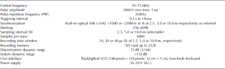
Since the first proposals for ice- and snow-penetrating radars (Reference CookCook, 1960) and their field implementation by Reference Evans and SmithEvans and Smith (1969), there have been many innovations in radar design, including those of Reference Matsuoka, Saito and NaruseMatsuoka and others (2004), Reference Mingo and FlowersMingo and Flowers (2010) and Reference Ye, Zhou, Wu, Zhao and FangYe and others (2011). In this paper we introduce a novel compact lightweight impulse ice-penetrating radar optimized for operating in a frequency range from 10 to 75 MHz (dependent on the antenna), with a high signal-to-noise ratio (SNR), a high transmitter power, a long recording time window, very low power consumption and storage capacity that allows for continuous recording of >250000 radar traces (i.e. >250 km of profiles at one trace m−1). Table 1 summarizes the capabilities of the radar. The system design allows it to be used for different geophysical measurements, such as common-offset profiling, common-midpoint (CMP) measurements or transillumination. It has a user-friendly interface. It can be operated easily on a snowmobile and sledge convoy or it can be carried in a backpack by a single person. The main system features are discussed in this paper. Further details can be found in Reference Machío RegidorMachío Regidor (2011)
Table 1. Main features of the radar system
System Design Considerations
The radar system consists of two main subsystems (Figs 1 and 2): the transmitter (TX) and the receiver (RX), with a synchronization system in between. For versatility and noise reduction purposes, the RX has been implemented as two separate modules: a receiver amplifier (RA), directly connected to the receiving antenna, and a control and recording unit (CRU).

Fig. 1. (a) The TX is connected to a power supply (12.6 V) and the transmitting antenna and receives a synchronization signal from the RX. The RX (CRU+ RA) controls the system and is connected to the receiving antenna, a power supply (12.6 V), a GPS receiver and a possible odometer, and transmits the synchronization signal to the TX. (b) The analog signal from the RA received at the CRU is 12-bit digitized, stacked and recorded using 16 bit per sample (four zero bits added) on the SD card.

Fig. 2. View of the radar system elements. The TX subsystem is shown on the left and the two units of the RX subsystem are shown in the centre (RA) and on the right (CRU).
Each module and the antennas were designed and developed from basic electronic components at the Universidad Politécnica de Madrid. Dimensions, masses and current consumptions of each unit are shown in Table 1. Two separate 10–20 V power supplies are needed, one for the CRU, through which the RA is powered, and the other for the TX. The most commonly used power sources are standard 12.6 V batteries. The dynamic range of the whole system including antennas (defined as the quotient of the peak power of the transmitter and the minimum power detectable by the receiver) is >132 dB.
Transmitter subsystem (TX)
The core of this subsystem is a pulse generator, triggered by the reception of a synchronization signal from the CRU. Several synchronization systems are possible, though the standard one is the optical synchronization link. Therefore, the TX unit includes both an optical synchronizing receiver as well as a connector for an external synchronization link, such as a radio signal (Fig. 2).
A previous version of the pulse generator was developed by Reference Vasilenko, Sokolov, Macheret, Glazovsky, Cuadrado and NavarroVasilenko and others (2002), which was inspired by an earlier one of Reference Wright, Hodge, Bradley, Grover and JacobelWright and others (1990). An array of eight avalanche transistors generates the pulse of the nonresonant impulse generator. Each transistor has its own power circuit, avoiding the need for high voltages within the unit. The peak-to-peak amplitude of the resulting pulse waveform is 2800 V with a rise time of 1 ns. The TX has a pulse-repetition frequency (PRF) of 20 kHz (i.e. pulse interval of 50 μs, allowing for a unique maximum range of ∼4 km of ice).
The rise time of this TX allows it to operate at frequencies up to 350 MHz. However, due to the high capacitance of low-frequency antennas, in practice, central frequencies lower than 10 MHz are not suitable.
Receiver subsystem (RX)
In this subsystem, which controls the radar, the RA has been implemented as a separate unit from the CRU to avoid noise generation in the receive signal. The RA is connected directly to the feed point at the centre of the receiving antenna. This allows use of the GPR with the receiving antenna separated from the CRU, thus increasing the versatility of the system.
Receiver amplifier module (RA)
This module consists of a symmetrical impedance-matching stage built using high-frequency low-noise bipolar transistors and an amplifier based on a high-performance single-chip solution (Analog Devices AD8367). The input impedance of the RA is ∼800Ω and the amplification can be set within the range 0–45 dB according to the particular needs (e.g. type of glacier ice, environmental noise level, type of antenna, etc.).
Control and recording unit module (CRU)
The CRU is the core of this ice-penetrating radar. It performs several functions, including synchronizing the pulse generation, sampling and digitizing the received signal, real-time stacking of signals, saving the resulting traces to memory and interfacing with the user for trace visualization and for setting the system parameters.
The block diagram of the CRU is shown in Figure 1b. The received signal from the RA is first sampled and digitized with a 12-bit analog-to-digital converter (ADC: Analog Devices AD9430), which has a maximum sampling frequency of 210 MHz. The digitized signal is then stacked and averaged in real time using a field programmable gate array (FPGA: Altera Cyclone EP1C12Q240I7N). A 16-bit micro-controller unit (MCU: Microchip dsPIC33F) is in charge of the management of synchronization, user interface input and output, and saves the resulting file on an SD card. The simulation and programming of our design on the FPGA was done using Quartus software from Altera, while the MCU has been configured and programmed in C, using the MPLAB C compiler from Microchip. The CRU circuits are implemented in three multilayer printed circuit boards (PCBs). The power supply and the interconnection PCBs are two-layered and the main CRU PCB is four-layered.
While the CRU is in recording mode, and until the arrival of a ‘stop recording’ command, each triggering signal initiates recording of a new trace and begins synchronization with the TX pulse generation. The triggering signal can be generated internally by a timer with user-selectable time-step from 0.1 s to 1 hour or through an external triggering signal. The latter can be generated by either an odometer or a manually operated switch.
We have implemented an optical synchronizing transmitter as a part of this module, although the 0183 (US National Marine Electronics Association) GGA (Global Positioning System Fix Data) standard sentences are then stored in the trace header. Storage using other synchronization can also be done externally (e.g. by radio link) using the connector provided. For trace-positioning purposes, an external GPS can be connected to the receiver, and NMEAGPS standards can be programmed if needed.
Each radar trace (Fig. 3) consists of 4000 samples of the signal. The sampling interval can be selected from one of 2.5, 5.0 or 10.0 ns (sampling frequency of 400, 200 or 100 MHz, respectively). The ADC employed restricts the sampling frequency to a maximum of 210 MHz. However, this radar includes an option of 400 MHz (sampling period 2.5 ns). In this case the CRU samples two consecutive signals at periods of 5 ns, with the second signal delayed by 2.5 ns. When the two traces are combined, an effective sampling interval of 2.5 ns is achieved. In order to reduce incoherent noise and increase the SNR, the CRU averages the signals in real time. The user can select the number of traces to include in the average, choosing from 2 n traces, where n = 8, 9,… 12 (i.e. stacking from 256 to 4096 traces). Following this process, an 8 kB trace, consisting of 4000 samples of the signal amplitude (2 bytes per sample) and a header (192 bytes), is saved to memory.

Fig. 3. An example of trace recorded using the 20 MHz antennas with a RX–TX separation of 12 m (Tavlebreen, Svalbard, April 2010). The amplitude is normalized by the maximum value of the recorded signal (in the figure, 91.55% of the saturation value). The zero of the two-way travel time (TWTT) is indicated by the red line. Because the direct wave through the air is the first arrival, TWTT = 0 occurs at a time before the onset of the direct wave given by the quotient between antenna separation and the radio-wave velocity in the air. The inset in the top right corner details the bedrock reflection. The high-frequency noise in the direct wave was induced on the large cables (∼2 m) used for connecting the GPS and the odometer to the CRU. It appears because of the large bandwidth of the system and could be avoided by diminishing the cable lengths or by adding a low-pass filter. Instead, we can implement low-pass filtering as a data-processing step (not done in the example shown).
A file is created whenever the first trace of a given profile is saved to memory, and is closed when a ‘stop recording’ command is issued. An SD memory card, up to 2 GB in size, is used by the CRU for storing traces. Therefore, it can store >250 000 traces (e.g. >250 km of profiles at one trace m−1).
The time needed to record a trace depends on the amount of stacking requested by the user. With high-speed SD cards, the trace-recording interval is 0.8 s for the highest stacking value (4096 traces). This time will be better than 0.3 s if the stacking number is 2048 or lower. At travel speeds of 4.5 km h−1, the system gathers one trace m−1 using a stacking number of 4096. At a travel speed of 12 km h−1 the user must choose a stacking number of 2048 or lower to achieve a horizontal trace spacing of 1 m.
The maximum sampling frequency of 400 MHz limits recording frequencies to values below 200 MHz. Taking into account the antenna bandwidth, antennas with central frequencies greater than 75 MHz are not suitable.
The CRU is located in a metal (aluminum) box to reduce external noise and interference. Its size, weight and power consumption are shown in Table 2. For ease of access, connectors, controls and screen are all located on the upper side of the box. Each connector is of a different type to avoid damage by accidental misconnection. The CRU has an interactive user interface menu to display the radar traces and to set the system parameter values using a very simple keyboard consisting of four knobs. The screen is a 12 cm × 7 cm (240 × 128 character) LCD with optional backlight. The main system settings, the GPS coordinates and the trace being recorded are shown on the LCD while profiling.
Table 2. Physical dimensions, mass and current consumption of the different modules of the radar system. The latter were measured with the system powered by standard batteries of 12.6 V. The consumption of the RX system with its LED backlight switched on (nonstandard use) is given in parentheses

We use the term recording time window to refer to the maximum time recorded in each trace. Because of the fixed number of samples per trace, the sampling period chosen also determines the maximum time window. The three allowed sampling intervals of 2.5, 5.0 and 10.0 ns result in recording time windows of 10, 20 or 40 μs, which allows sampling ice depths of 800, 1600 and 3300 m, assuming a radio-wave velocity in ice of 0.168 m ns−1 .
Antennas
The antennas follow the Wu–King design (Reference Wu and KingWu and King, 1965; corrections by Reference Shen and KingShen and King, 1965). We have built two sets of flexible lightweight 80%-resistively loaded dipoles, with central frequencies of 20 and 75 MHz. Their corresponding lengths are 5.8 and 1.7 m, and masses are 450 and 200 g, respectively. Each dipole consists of 18 resistors and 20 metal wires, all of them cored by a polypropylene cable, allowing us to tie the antennas to the sledge or slings.
Synchronization
The pulse generation by the TX is triggered by the arrival of a synchronization signal from the CRU of the RX, starting the recording of each new trace. This synchronization is achieved by means of an optical link. The synchronization transmitter is located in the CRU of the RX, while the synchronization receiver is located in the TX.
Once the CRU starts recording (zero time of the trace), the synchronization signal is sent from the CRU to the TX, at which time the TX transmits its pulse. This time we define as the zero time of the TWTT (Fig. 3). The delay associated with the transit of the synchronization signal through the optical cable effectively shortens the recording time window. As a result, optical cables of 500, 1000 and 2000 m in length should be used according to recording time windows of 10, 20 or 40 μs, respectively. Such cable lengths are especially useful for measurement techniques such as CMP or transillumination. However, for common-offset profiling, as is commonly done from sledge- or backpack-based work, an optical cable length of 15 m is sufficient.
An alternative synchronization by means of a radio link is also available through dedicated connectors implemented in both the CRU of the RX, and the TX. However, the optical link is more reliable and should be used whenever the field configuration can support a physical connection between the TX and the RX.
Field Operation
The system can be operated in the field in different configurations, such as a snowmobile and sledge convoy or walking. The system units are interconnected as shown in Figure 1a. Figure 4 shows a possible field configuration for a parallel end-fire common-offset profiling, in which the convoy consists of a snowmobile pulling two sledges. At the end of the convoy, a friction element pulled by a rope acts as a brake, keeping the trailing dipole extended. Usually, a second snowmobile is located at the end of the convoy. In addition to keeping the antenna extended, this provides additional security, acting as a retaining element should the leading scooter fall into a crevasse. In backpack-mounted profiling by a single operator, it is convenient to place the CRU in front of the operator in a chest-mounted harness and the RA is kept separate from the CRU at the centre of the receiving antenna. The TX must also be towed by the operator. Skis or small sledges can be used for this purpose, depending on snow/ice conditions.
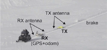
Fig. 4. Profiling during spring 2010 field tests in Svalbard using the 20 MHz antennas. A single scooter is leading the convoy, with the RX and TX placed on separate small sledges. An odometer is placed on the leading sledge.
As mentioned, the default TX–RX synchronization uses an optical cable link. Optical fiber cables are nowadays strong and flexible enough for field campaign use. Since 2003 we have successfully used 3 mm single-mode SM 10/125 optical fiber that allows up to 200 N of traction (350 N of instantaneous traction) and has a curvature radius of 45 mm. If sharper bends are introduced, the optical cable does not break, though signaling is interrupted. Simply straightening the cable restores the synchronization. When profiling in common-offset configuration, and depending on the roughness of the ice/snow cover, we either loosely tie the optical cable to the main traction rope, protect it in a lightweight corrugated plastic pipe or hold the cable above the ground using poles at the TX and RX locations. No special care is needed with the optical fiber when recording a CMP measurement.
To start recording, the operator must select the triggering system (timer, odometer, manual) and the corresponding triggering period/distance, the number of signals that must be averaged to build each recorded trace (stacking number), the sampling frequency and the name of the profile. Once the recording starts, each time the operator stops it, a new file is saved and the filename is automatically incremented by one unit. In this way, the typical operation during glacier profiling is limited to pushing the start/stop button at the start and end points of each profile and checking the proper working of the system. Of course, the system parameters and the filename can be set independently for each profile.
Field Tests
The complete radar system was tested in Svalbard during the spring of 2010 and 2011. Prototype versions of some of its modules were tested in earlier campaigns. The field tests of April 2010 were made on Tavlebreen (77°58′ N, 15°07′ E), a polythermal glacier in Spitsbergen. Figure 4 shows the set-up used during these field tests. In April 2011 measurements were undertaken on Hansbreen (77°04′ N, 15°35′ E), Recherchebreen (77°25′ N, 14°52′ E), Hogstebreen (77°20′ N, 15°05′ E) and Amundsenisen (77°18′ N, 15°30′ E), a set of polythermal/temperate glaciers/ice fields in Spitsbergen. The bedrock was reached in all cases. A sample profile is shown in Figure 5. On Amundsenisen we clearly detected the bed under ∼690 m of temperate ice. This is the thickest ice that we have surveyed so far. Considering the strong scattering in temperate ice and the quality of our records, we estimate that in cold ice we would be able to image up to the limit imposed by the recording time window (40 μs, i.e. ∼3300 m depth).
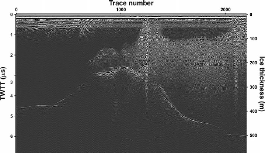
Fig. 5. An example of a radar profile recorded using the 20 MHz antennas (Recherchebreen and Hogstebreen, Svalbard, April 2011). The left axis shows the TWTT while the right axis displays the ice thickness, assuming a radio-wave velocity of 0.168 m ns−1. Bedrock is clearly visible below 500 m of wet ice.
Concluding Remarks
We have designed and implemented a compact lightweight impulse GPR for glaciological applications. Notable features include real-time stacking of up to 4096 traces to build a final trace. This stacking capability, along with the high transmitted power (peak voltage 2800 V) and stable transmitter, provides a dynamic range of the whole system larger than 132 dB. Such features combined with the large recording time window available (up to 40 μs) make this radar suitable for sounding thick temperate ice.
The system memory uses removable standard SD flash cards (up to 2 GB). This gives the radar the capability to record, without interruption, >250 km of profiles at a rate of one trace m−1. If a larger storage capacity is required, all that is needed is to replace the SD card. If such a rate is aimed for, profiling velocities of 12 km h−1 can be reached using stacking values up to 2048.
To avoid coupling effects or interference with the antennas, the system uses, by default, an optical synchronization link although other external synchronization systems are also possible (e.g. by radio link). Distances between the TX and RX up to 2000 m are possible, thus allowing many kinds of geophysical measurements (common-offset profiling, CMP, transillumination, etc.).
The entire system can be operated by a single person. Owing to its modularity, low weight and low power consumption, this radar can be carried easily in a backpack. Profiling for >7 hours is possible with a total system weight of <9 kg including antennas and batteries.
Acknowledgements
This research was supported by grant CTM2008-05878/ANT from the Spanish Ministry of Science and Technology (National Plan for R&D). We thank the crews of the research station of the Russian Academy of Sciences in Barentsburg and the Polish Polar Station in Hornsund, both in Svalbard, for their support in our field tests. We thank two anonymous reviewers whose comments and suggestions substantially improved the manuscript. We also thank S. Anandakrishnan for his technical comments and review of the writing style.


