


1. INTRODUCTION
Iceberg calving from marine-terminating glaciers and ice shelves accounts for ~50% of the mass lost from both the Greenland and Antarctic ice sheets (Jacobs and others, Reference Jacobs, Hellmer, Doake, Jenkins and Frolich1992; Bigg, Reference Bigg1999; Rignot and others, Reference Rignot2008, Reference Rignot, Jacobs, Mouginot and Scheuchl2013; Logan and others, Reference Logan, Catania, Lavier and Choi2013; Liu and others, Reference Liu2015). Calving from floating ice shelves or ice tongues can critically disrupt the stability of ice sheets and glaciers by diminishing the ice shelves' buttressing force and promoting further retreat and glacier speed up (MacGregor and others, Reference MacGregor, Catania, Markowski and Andrews2012). However, calving is a natural process that occurs when a combination of surface and basal crevasses (fractures) propagates through the entire thickness of the ice shelf or glacier, leading to the formation of icebergs. Hydro-fracture, the process in which ice is fractured by the pressure of water in crevasses, plays an important role in iceberg calving in marine-terminating glaciers, and the calving rate has been linked to surface meltwater availability and warm ocean waters (Benn and others, Reference Benn, Warren and Mottram2007; Nick and others, Reference Nick, der Veen, Vieli and Benn2010). DeConto and Pollard (Reference DeConto and Pollard2016) argued that contributions of at least a meter to sea-level rise within the 21st and 22nd century are plausible when iceberg calving is linked to climate dynamics through processes such as hydro-fracturing in surface and basal crevasses. Given the broader societal implications that calving has for future sea-level rise, researchers have recently used linear elastic fracture mechanics (LEFM) models in conjunction with numerical ice-sheet models to improve the simulation of crevasse propagation and iceberg calving (Krug and others, Reference Krug, Weiss, Gagliardini and Durand2014; Yu and others, Reference Yu, Rignot, Morlighem and Seroussi2017). The objective of this paper is to investigate (using the finite element method) whether the evaluation of the stress intensity factor in the calving (or crevasse) models using LEFM (van der Veen, Reference van der Veen1998a, Reference van der Veenb; Krug and others, Reference Krug, Weiss, Gagliardini and Durand2014) is appropriate for grounded glaciers and floating ice shelves.
The LEFM approach to modeling the propagation of fractures in brittle materials is based on the mathematical theory of elasticity, which states that the stresses asymptotically tend to infinity at the crack tip (i.e., stress singularity). A material cannot realistically sustain infinite stress, and in true scenarios, the stresses close to the crack tip are bounded by a plastic or cohesive zone (Dugdale, Reference Dugdale1960). Even so, if the size of the plastic zone is sufficiently small (e.g., as in brittle failure of ice), then LEFM is appropriate for describing fracture propagation. According to LEFM theory (Griffith, Reference Griffith1921), the crack grows when the strain energy released by crack propagation is equal to the surface energy required to expand the crack. The so-called Griffith energy or critical strain energy release rate is a material property that represents the energy released per unit distance as the crack grows. In practice, however, it is more common to describe crack growth in terms of the stress intensity factor (SIF) in relation to the critical SIF (also called fracture toughness), which is a material property inherently related to the Griffith energy. The stress intensity factor (not to be confused with the stress concentration factor) was introduced by Irwin (Reference Irwin1957) to characterize the state of stress within the vicinity of a crack tip in an elastic material under applied loading. The SIF is a function of the loading conditions, domain geometry, crack orientation, and crack size and is directly proportional to the applied stress and the square root of crack size. The crack will propagate when the SIF is greater than the critical SIF, thus providing a simple failure criterion for brittle materials. However, it is questionable whether LEFM is appropriate for modeling crevasse or rift propagation in glacier ice, whose nonlinear viscous rheology is better described by the Glen's flow law over long timescales (Cuffey and Paterson, Reference Cuffey and Paterson2010). In this context, damage mechanics approaches hold promise for modeling creep fracture in viscous/viscoelastic ice (Pralong and Funk, Reference Pralong and Funk2005; Duddu and Waisman, Reference Duddu and Waisman2013; Mobasher and others, Reference Mobasher, Duddu, Bassis and Waisman2016; Jiménez and others, Reference Jiménez, Duddu and Bassis2017), but they are computationally more expensive than the LEFM approaches.
Despite its limitations, the SIF-based LEFM approach has been widely applied by the glaciology community to predict the penetration depth of water-filled crevasses through glaciers (see Colgan and others, Reference Colgan2016, for an in-depth review). The advantage of the LEFM models is that they provide both a physical basis for estimating crevasse penetration depths and computational efficiency for implementation into numerical ice-sheet models. Smith (Reference Smith1976) first proposed a simple LEFM model for estimating the penetration depth of water-filled crevasses based on the assumption that ice thickness is infinite, but it is applicable only when the crevasse depth is much less than the ice thickness. To account for the finite ice thickness of glaciers, van der Veen (Reference van der Veen1998a, Reference van der Veenb) proposed a LEFM model that incorporated weight functions into the SIF evaluation, as given by Tada and others (Reference Tada, Paris and Irwin1973, Reference Tada, Paris and Irwin2000). Recently, Krug and others (Reference Krug, Weiss, Gagliardini and Durand2014) employed a more accurate weight function into the SIF evaluation, as given by Glinka and Shen (Reference Glinka and Shen1991); Moftakhar and Glinka (Reference Moftakhar and Glinka1992a). However, these weight functions were originally formulated for evaluating the SIF for a rectangular, finite-width plate with a single edge-crack subjected to far-field uniaxial normal stress, which may not be suited for crevasses within grounded glaciers or ice shelves owing to differences in boundary conditions. Therefore, in this paper, we investigate the appropriateness of the SIF functions used in van der Veen (Reference van der Veen1998a, Reference van der Veenb); Krug and others (Reference Krug, Weiss, Gagliardini and Durand2014), for water-filled surface and basal crevasses in idealized rectangular ice slabs with different basal boundary conditions.
The rest of the paper is organized as follows: first, we will review the weight function method, the equations for evaluating the SIF in van der Veen (Reference van der Veen1998a, Reference van der Veenb) and Krug and others (Reference Krug, Weiss, Gagliardini and Durand2014) LEFM models and the finite element method-based evaluation of the SIF using the displacement correlation method (Gupta and others, Reference Gupta, Duarte and Dhankhar2017); second, we will compare the SIFs computed numerically against those calculated from the analytical LEFM models and illustrate their suitability in relation to the basal boundary condition; finally, we will provide a few concluding remarks regarding the modeling of calving in ice-sheet models. Thus, we explore the reasons for the discrepancy between analytically and numerically evaluated SIFs in existing crevasse/calving models using LEFM and we address the broader implications of this discrepancy for calving models applied to grounded glaciers with different basal boundary conditions and floating ice shelves.
2. LEFM MODELS AND METHODS
2.1. Stress state in ice
Throughout this paper, we consider a rectangular ice slab with height H and length L with water-filled surface and/or basal crevasses, as depicted in Figure 1. Typically, crevasse opening is regarded as mode I fracture driven by the longitudinal (horizontal) normal stress σ xx through the ice thickness, which is dependent on the boundary conditions. In a freely floating ice shelf (i.e., no tangential traction at the base), the far-field horizontal Cauchy (normal) stress σ xx varies linearly with depth, assuming that ice is incompressible and the Glen's law viscosity coefficient is a constant (Weertman, Reference Weertman1957). This longitudinal stress can be decomposed into ‘resistive’ and lithostatic components as (van der Veen, Reference van der Veen1998a)
 $$\sigma_{xx}(z) = R_{xx} - \rho_{\rm i} g \left\langle H-z \right\rangle, $$
where R xx is the so-called resistive stress which is directly related to the deviatoric stress, ρ i is the density of ice, g is the acceleration due to gravity, z is the vertical coordinate measured from the bottom of the domain, and the Macaulay brackets 〈x〉 = (|x| + x)/2. The resistive stress becomes constant with depth in the ‘far-field’ region of the domain (i.e., far from the terminus and the grounding line) and can be determined by applying a depth-integrated force balance, that is, we equate the depth-integrated Cauchy stress with the depth-integrated terminus pressure (Bassis and Walker, Reference Bassis and Walker2012) to obtain
 $$R_{xx} = {1 \over 2} \rho_{\rm i} g H - {1 \over 2} \rho_{\rm w} g {h_{\rm w}^2 \over H}, $$
where ρ w = 1020 kg m−3 is the density of seawater and h w is the seawater depth at the glacier terminus. The key concept here is that the far-field normal stress and the resistive stress are constitutively independent so long as incompressibility of ice deformation is assumed. Consequently, a linear elastic material model is sufficient to describe the stress state in ice in the far-field regions.
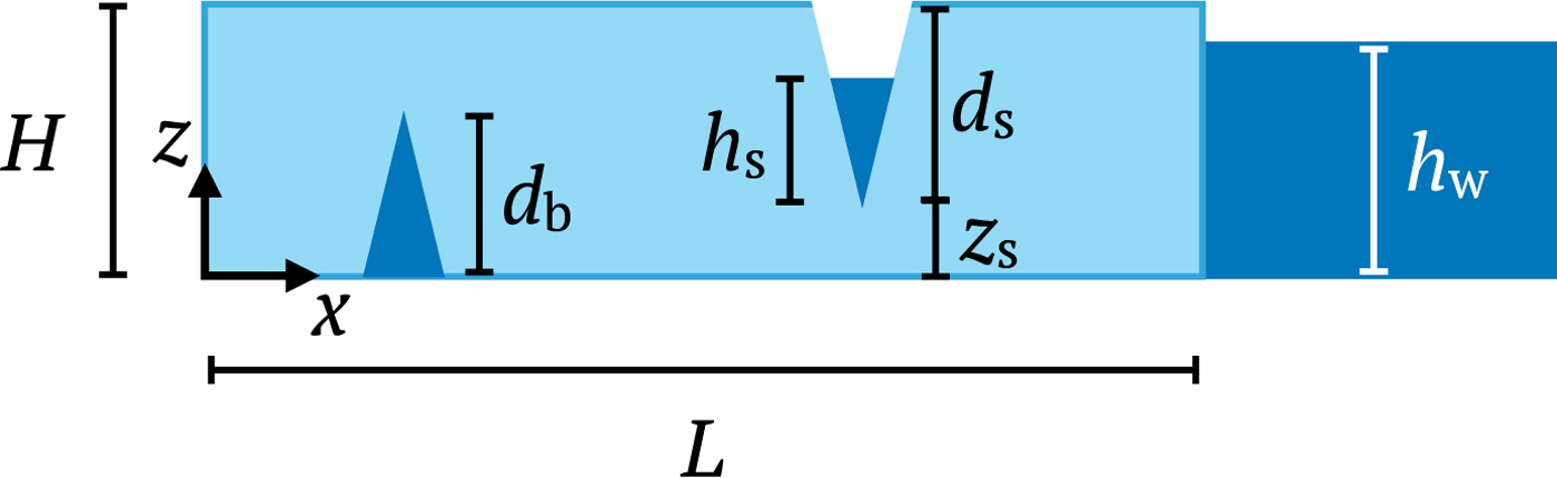
Fig. 1. Rectangular glacier with height H, length L, seawater level h w, surface crevasse depth d s, water level h s within the surface crevasse and basal crevasse depth d b. The origin is set at the lower-left corner with x and z denoting the horizontal and vertical coordinates, respectively.
To account for the hydraulic pressure exerted on the crack walls in water-filled crevasses, we introduce an additional loading term
 $$\sigma_{\rm w}(z) = \left\{ \matrix{\rho_{\rm w} g \langle{h_{\rm s} - (z - z_{\rm s})}\rangle, & \hbox{in surface crevasses} \cr \!\!\!\!\!\!\!\!\!\!\!\!\!\rho_{\rm w} g \langle{h_{\rm w} - z}\rangle, &\!\! \hbox{in basal crevasses},} \right. $$
where h s and z s are the water height within the surface crevasse and the vertical coordinate of the surface crevasse tip, respectively. Because the hydraulic pressure acts to open the crack walls, it is assumed that σ w exerts a positive (tensile) stress. The net longitudinal stress that causes crevasse opening is given by (Jezek, Reference Jezek1984; Nick and others, Reference Nick, der Veen, Vieli and Benn2010; Bassis, Reference Bassis2011)
 $$\eqalign{\sigma_{\rm net}(z) & = \sigma_{xx}(z) + \sigma_{\rm w}(z) \cr &= R_{xx} - \rho_{\rm i} g \left\langle H-z \right\rangle + \sigma_{\rm w}(z)}$$
Equations (1)–(4) are still valid for an idealized rectangular grounded glacier with free-slip (i.e., no tangential traction) at the base and without any lateral drag from the sides (van der Veen, Reference van der Veen1998a); however, these equations are not valid for a rectangular grounded glacier that is either frozen to the bedrock or subjected to basal friction.
2.2. Weight function method
In the analytical LEFM models, the stress intensity factor (SIF) is often calculated using the weight function method (Bueckner, Reference Bueckner1970; Rice, Reference Rice1972). The mode I SIF, denoted K I, is evaluated by integrating a generic weight function m(z, t, d) and the normal stress σ(z) along the potential crack surface over its length d as (Glinka and Shen, Reference Glinka and Shen1991)
 $$K_{\rm I} = \int_{0}^{d} m(z,t,d)\sigma(z) \; {\rm d}z. $$
where t is a geometry parameter (e.g., width or thickness) of the cracked body. This method can be extended to problems where the loading is applied not just on the crack surface, but also on the exterior boundaries using the principle of linear superposition. As shown in Figure 2, the linear elastic stress state in Case a (with a traction-free crack and applied far-field stress) can be obtained by superposing the stress state in Case b (without a crack and applied far-field stress) and Case c (with traction loading only on the crack surface). Therefore, the SIF at the tip of the crack in Case a is equal to the SIF in Case c, so it can be computed using (5) if the appropriate weight function is known. Petroski and Achenbach (Reference Petroski and Achenbach1978) proposed a general method for deriving the weight function m(z, t, d), which was later extended by several researchers to improve the accuracy of SIF evaluation (see Glinka and Shen Reference Glinka and Shen1991 for more details). Thus, the advantage of the weight function method is that the SIF for any complex stress field applied to the body can be easily calculated by (numerical) integration; however, it is important to note that the weight function should be determined appropriately for the particular geometry of the cracked body and boundary conditions.
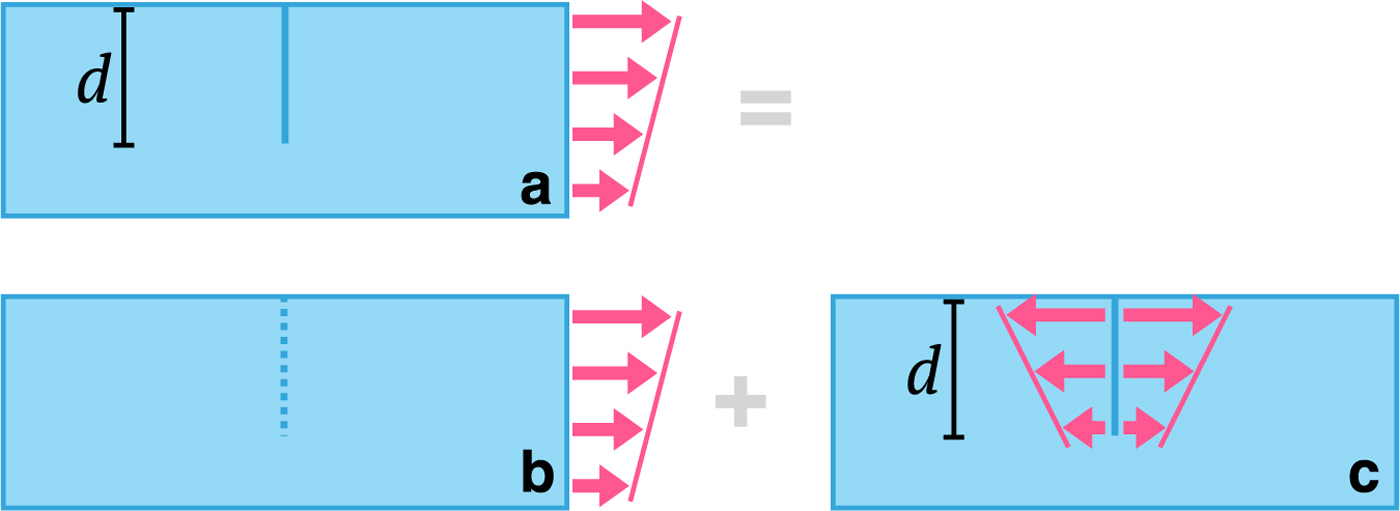
Fig. 2. Superposition principle demonstrated in domains a, b and c. The dashed line in domain b indicates a potential crack surface.
From a glaciology standpoint, three idealized cases of a finite-thickness cracked rectangular slab becomes relevant in two dimensions:
(1) the single edge crack case, shown in Figure 3(a), which represents a surface or basal crevasse in a floating ice tongue or ice shelf;
(2) the central through crack case, shown in Figure 3(b), which represents a basal crevasse in a grounded glacier with free tangential slip;
(3) the double edge cracks case, shown in Figure 3(c), which represents a surface crevasse in a grounded glacier with free tangential slip.
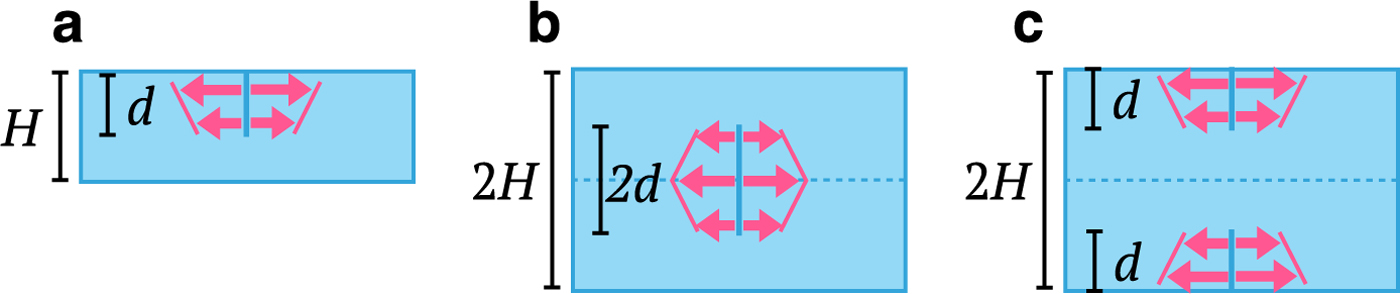
Fig. 3. (a) Single edge crack, (b) central through crackand (c) double edge cracks through finite slabs of width H with crack length d. The magenta arrows indicate applied loading on the crack surface. The (dashed) lines of symmetry in (b) and (c) represent the free slip basal surface of the glacier.
We note that the single edge crack case is not an exact analogy to a crevasse in a floating ice shelf because of the buoyancy force on the basal boundary. We also note that in the central through crack and double edge cracks cases, the horizontal line of symmetry represents the free slip basal surface of the glacier. In the following sections, we will describe three analytical LEFM models for evaluating crevasse penetration depths in grounded glaciers and floating ice shelves that employ different weight functions derived for the single edge crack case. In Appendix A, we provide the weight functions m C(z, H, d) and m D(z, H, d) corresponding to the central through crack and double edge cracks cases, respectively.
2.3. van der Veen (Reference van der Veen1998a) LEFM model
The LEFM model presented by van der Veen (Reference van der Veen1998a) was originally applied to determine the penetration depth of dry and water-filled surface crevasses in glaciers. For an assumed crevasse penetration depth d s, the net mode I SIF  $K_{\rm I}^{\rm net}$ at the crack tip can be evaluated as
 $$K_{\rm I}^{\rm net} = K_{\rm I}^{(1)}(R_{xx}, d_{\rm s}) + K_{\rm I}^{(2)}(d_{\rm s}) + K_{\rm I}^{(3)}(h_{\rm s}, d_{\rm s}), $$
where  $K_{\rm I}^{(1)}$, $K_{\rm I}^{(2)}$ and $K_{\rm I}^{(3)}$ are the SIFs resulting from the resistive stress, ice overburden pressure and water pressure within the crevasse, respectively. Using the weight function method, these terms can be evaluated as
 $$K_{\rm I}^{(1)} = F(\lambda) R_{xx} \sqrt{\pi d_{\rm s}}, $$
 $$K_{\rm I}^{(2)} = \int_0^{d_{\rm s}} \left[ {-2 \rho_{\rm i} g z^\prime \over \sqrt{\pi d_{\rm s}}} G(\lambda, \gamma) \right] {\rm d}z^\prime, $$
 $$K_{\rm I}^{(3)} = \int_{0}^{d_{\rm s}} \left[ {2 \rho_{\rm w} g \langle z^\prime - h' \rangle \over \sqrt{\pi d_{\rm s}}} G(\lambda, \gamma) \right] {\rm d}z^\prime, $$
where z′ = H − z is the vertical coordinate measured from the top of the glacier, and the depth of the dry portion of a water-filled crevasse h′ = d s − h s. Because the resistive stress R xx is not a function of depth, (7) gives the integrated weight function F(λ). The expressions for the weight functions F(λ) and G(λ, γ) are provided in Appendix B. The parameters λ = d s/H and γ = z′/d s, and thus λ accounts for finite domain size (i.e., ice thickness). It is important to note that these weight functions were originally derived for a rectangular finite-width plate with a single edge crack under applied far-field normal stress (Tada and others, Reference Tada, Paris and Irwin1973, Reference Tada, Paris and Irwin2000), as depicted in Figure 3(a), so they are not generally applicable for all loading configurations and domain boundary conditions.
2.4. van der Veen (Reference van der Veen1998b) LEFM model
The LEFM model presented by van der Veen (Reference van der Veen1998b) was originally applied to determine the penetration depth of water-filled basal crevasses in glaciers. The key difference between the van der Veen (Reference van der Veen1998a) and van der Veen (Reference van der Veen1998b) models is that the latter only uses the weight function G(λ, γ) and applies it to the net Cauchy stress σ net defined in (4). Using the weight function method the net SIF is evaluated as
 $$K_{\rm I}^{\rm net} = \int_{0}^{d_{\rm b}} \left[ 2 {\sigma_{\rm net}(z) \over \sqrt{\pi d_{\rm b}}} G(\gamma, \lambda) \right] \; {\rm d}z. $$
In the above equation, we can numerically integrate the integrand along the depth of the basal crevasse, that is, from the base of the glacier at z=0 to the tip of the basal crevasse at z = d b. The equation may also be applied to compute  $K_{\rm I}^{\rm net}$ at the tip of a water-filled surface crevasse by integrating along the depth of the surface crevasse, that is, from the tip of the surface crevasse at z = z s to the top surface of the glacier at z=H.
2.5. Krug and others (Reference Krug, Weiss, Gagliardini and Durand2014) LEFM model
The LEFM model applied by Krug and others (Reference Krug, Weiss, Gagliardini and Durand2014) is similar to the van der Veen (Reference van der Veen1998b) model in that the net Cauchy stress is multiplied by a single weight function and integrated over the depth of the crack to obtain the net SIF. Thus, using the weight function method, net SIF at the tip of a surface crevasse is calculated as
 $$K_{\rm I}^{\rm net} = \int_{0}^{d_{\rm s}} \beta(z',H,d_{\rm s}) \sigma_{\rm net}(z') \; {\rm d}z' $$
and at the tip of a basal crevasse is calculated as
 $$K_{\rm I}^{\rm net} = \int_{0}^{d_{\rm b}} \beta(z,H,d_{\rm b}) \sigma_{\rm net}(z) \;{\rm d}z $$
where β is the universal weight function provided in Appendix C (Glinka, Reference Glinka1996). The term ‘universal weight function’ is slightly deceiving here because the parameters M i in the expression for β (see Appendix C) change with the geometry and boundary conditions of the cracked body. Moftakhar and Glinka (Reference Moftakhar and Glinka1992b) reported different high-order polynomial functions for the parameters M i using the least squares fitting technique to match the weight functions corresponding to different geometries of the cracked body and boundary conditions (i.e., symmetric versus unsymmetric plates). Although the LEFM model discussed in Krug and others (Reference Krug, Weiss, Gagliardini and Durand2014) used the universal weight function, it only considered the parameters M i for the single edge crack case for a rectangular slab with finite thickness, as depicted in Figure 3(a).
2.6. Displacement correlation method
The displacement correlation method (DCM) is a simple technique for computing the SIF at the crack tip using the crack opening displacements obtained from the finite element method (Banks-Sills and Sherman, Reference Banks-Sills and Sherman1986). For an isotropic, homogeneous linear elastic solid, the SIF can be approximated as
 $$K_{\rm I}^{\ast}(r) = \sqrt{{2 \pi \over r}} {\mu \over \kappa + 1} [\![u_n(r)]\!], $$
where  $[\![u_n(r)]\!] = u_n^{+}(r) - u_n^{-}(r)$ is the jump in the normal component of the displacement across the crack surface (i.e., crack opening displacement) and is computed by taking the difference between normal displacements $u_n^{+}(r)$ and $u_n^{-}(r)$ along opposing crack surfaces at a distance r from the crack tip. The parameter μ = E/(2(1 + ν)) is the shear modulus; E is the Young's modulus; ν is the Poisson's ratio; and κ = 3 − 4ν is the Kolosov constant. In the above equation, the * in the superscript indicates that the SIF approximation has first order accuracy (i.e., ${\cal O}(r)$ error). However, by applying a Richardson extrapolation (Heath, Reference Heath1997), the SIF can be computed with second order accuracy (i.e., ${\cal O}(r^2)$ error) as
 $$K_{\rm I}^{\rm net} = K_{\rm I}^{\ast}(r_{\rm a}) + {r_{\rm a} \over r_{\rm b} - r_{\rm a}} \left( K_{\rm I}^{\ast}(r_{\rm a}) - K_{\rm I}^{\ast}(r_{\rm b}) \right), $$
where  $K_{\rm I}^{\ast}(r_{\rm a})$ and $K_{\rm I}^{\ast}(r_{\rm b})$ are the SIFs (with first order accuracy) computed at two different locations with radii r a and r b, where r b > r a. To compute the SIF using the DCM in conjunction with the finite element method, we first solve the governing equations of the elasticity boundary value problem in the rectangular ice domain and obtain the displacement vector field u at the finite element nodes. Next, we compute the crack opening displacement $[\![ u_n(r) ]\!] = [\![{\bi u}(r) ]\!] \cdot {\bi n}$ at any two locations r = r a and r = r b along the crack, where n is the unit vector normal to the crack interface and the dot (·) denotes the scalar product of vectors. Finally, we apply (13) and (14) to compute $K_{\rm I}^{\rm net}$. The advantage of the DCM is that it is simpler to implement than the J-integral (Rice, Reference Rice1968) and gives consistent results even when the crack surfaces are subjected to hydraulic pressure (Gupta and Duarte, Reference Gupta and Duarte2018). For a more detailed review of the DCM and its advantages over other numerical techniques for SIF evaluation, the reader is referred to Gupta and others (Reference Gupta, Duarte and Dhankhar2017).
3. NUMERICAL RESULTS
In this section, we compare the net SIFs calculated from the calving models using LEFM (van der Veen, Reference van der Veen1998a,Reference van der Veenb; Krug and others, Reference Krug, Weiss, Gagliardini and Durand2014) against the net SIFs calculated using the DCM in conjunction with finite element analysis for crevasses in grounded glaciers and floating ice shelves. For grounded glaciers, we consider two extreme scenarios for the basal boundary condition, namely, free slip along the flat bedrock surface and fixed (i.e., frozen) to the bedrock surface. We also consider different seawater depths at the terminus for marine-terminating grounded glaciers. For conducting finite element analysis, we utilize the open source software FEniCS (Alnæs and others, Reference Alnæs2015) and apply mixed-order finite elements to avoid volumetric locking resulting from the incompressibility of ice deformation. We use a total-Lagrangian reference frame so as to be consistent with the small deformation assumption of analytical LEFM models. The material properties for incompressible, linear elastic ice are taken as follows: the elastic modulus E = 9500 MPa, the Poisson's ratio ν = 0.5, and the density of ice ρ i = 917 kg m−3. To obtain the SIF from the analytical models, we apply (5)–(12) and employ Simpson's rule for numerical integration. For the single edge crack case, we utilize the weight functions described in the calving models (van der Veen, Reference van der Veen1998a, Reference van der Veenb; Krug and others, Reference Krug, Weiss, Gagliardini and Durand2014); whereas for the double edge cracks and central through crack cases, we apply (5) and substitute in the appropriate weighting functions m D(z, H, d) and m C(z, H, d) from Appendix A.
3.1. SIF evaluation in grounded glaciers with free slip at the base
Our aim in this section is to demonstrate using the finite element method and the DCM that the SIFs calculated by the LEFM models of van der Veen (Reference van der Veen1998a, Reference van der Veenb); Krug and others (Reference Krug, Weiss, Gagliardini and Durand2014) are consistent with the edge-loaded cantilever beam configuration, but are not consistent with the gravity-loaded grounded slab configuration. Instead, the SIFs calculated from the double edge cracks case is consistent with the gravity-loaded grounded slab configuration. In each finite element simulation, we consider an idealized, rectangular domain with length L = 1000 m and height H = 125 m under plane strain assumptions (i.e., the out-of-plane component of strain is zero). The domain is subjected to either of the following two loading configurations:
(1) The gravity-loaded grounded slab configuration, wherein we apply free-slip boundary conditions at the left and bottom edges of the domain (indicated by rollers) and apply gravity loading as a body force with magnitude ρ ig in the vertical direction, as illustrated in Figure 4(a). In the case when seawater pressure is acting at the glacier terminus, we apply a hydrostatic load with hydraulic head h w to the right domain edge as a depth-varying (triangularly) distributed load. This loading configuration has glaciological significance as it represents a land or marine-terminating glacier resting over a free-slip surface and deforming under its self-weight. We also note that this gravity-loaded grounded slab configuration is equivalent to the top half of the symmetric domain with double edge cracks in Figure 3(c), because there can be no vertical displacement at the line of symmetry, but horizontal displacement is allowed.
(2) The edge-loaded cantilever beam configuration, wherein we apply a free-slip boundary condition at the left domain edge and apply a depth-varying stress σ xx(z, h w) to the right domain edge as a traction boundary condition, as illustrated in Figure 4(b). Therefore, the horizontal Cauchy stress along any vertical section is given by (1) because there are no applied body forces. To prevent rigid body translation we restrain or pin the bottom left corner (indicated by a triangle). Applying the superposition principle, we can show that this loading configuration is equivalent to the finite-thickness slab with a single edge crack as shown in Figure 3(a) for the purpose of evaluating the SIF at the crack tip. This loading configuration has some glaciological significance as it represents a floating ice tongue deforming under its self-weight; however, a major difference is that basal boundary of the floating ice shelf has normal traction due to buoyancy.

Fig. 4. Loading configurations for the (a) gravity-loaded slab and (b) loaded cantilever beam with H = 125 m and L = 1000 m. The horizontal Cauchy stress σ xx contour resulting from the gravity-loaded slab and loaded cantilever beam configurations are shown in Subfigures (c) and (d), respectively, when d s = 0.
The contour plots of longitudinal stress σ xx obtained through finite element analysis for the gravity-loaded grounded slab and edge-loaded cantilever beam configurations are shown in Figs. 4(c) and 4(d), respectively. We note that in the far-field (i.e., away from the terminus), σ xx resulting from both loading configurations is identical and has the same linear variation with depth, described by (1). However, in the gravity-loaded slab configuration, the stress distribution is locally affected by the traction-free edge at the terminus. Therefore, for each simulation we position the surface (or basal) crevasse at the point x = L/2, which is sufficiently far from the terminus so that the edge effects vanish. Even though the far-field stress is identical for both configurations, the deformation of the domain and the displacement jump across the crack surface is quite different as shown in Figure 5. Next, to account for water within the crevasse, we apply hydrostatic pressure as a Neumann boundary condition normal to the crack walls in the simulation studies; whereas, in the LEFM models, we assume that the net horizontal Cauchy stress is given by the expression in (4) based on the linear superposition principle, as done in van der Veen (Reference van der Veen1998a, Reference van der Veenb); Nick and others (Reference Nick, der Veen, Vieli and Benn2010).

Fig. 5. Deformed shapes of (a) the gravity-loaded slab configuration and (b) the loaded cantilever beam configuration. The purpose of these plots is to show qualitatively the deformed configuration and the crack tip opening. We, therefore, do not show the color bar for the stress contours.
We now present the net SIF versus crevasse depth curves for three different cases: dry surface crevasses and water-filled surface and basal crevasses. In Figure 6–8, we plot  $K_{\rm I}^{\rm net}$ at the crack tip for different surface crevasse depths d s and different basal crevasse depths d b for the two previously described loading configurations. In Figure 6, we plot $K_{\rm I}^{\rm net}$ for dry surface crevasses considering two different seawater depths h w = 0% and h w = ρ i/ρ w ≈ 90% at the terminus (i.e., near-floating); in Figs. 7 and 8, we plot $K_{\rm I}^{\rm net}$ for water-filled surface crevasses and water-filled basal crevasses, respectively, with the near-floating condition at the terminus. The water-filled surface crevasses are fully filled (i.e., h s/d s = 100%), and the water-filled basal crevasses have a hydraulic head of h w. The three LEFM models (van der Veen, Reference van der Veen1998a, Reference van der Veenb; Krug and others, Reference Krug, Weiss, Gagliardini and Durand2014) show good agreement with each other, but the van der Veen (Reference van der Veen1998a) model diverges in the h w/H = 0% case with dry surface crevasses (see Fig. 6) owing to the discrepancy in the use of the weight functions. The numerically extracted $K_{\rm I}^{\rm net}$ using the DCM in the edge-loaded cantilever beam configuration shows excellent agreement with the three LEFM models; whereas, the numerically extracted $K_{\rm I}^{\rm net}$ in the gravity-loaded grounded slab configuration shows better agreement only when using the weight functions for the double edge cracks and central through crack cases for surface and basal crevasses, respectively. We also make the following observations regarding crevasse propagation and calving:
(1) the SIFs predicted by the DCM and double edge crack for dry surface crevasses in land-terminating glaciers (i.e., h w/H = 0%) are positive only for d s/H < 95% (see Fig. 6), so full depth crevasse propagation is not likely to occur (calving does not occur);
(2) the SIFs predicted by all the LEFM models and the DCM for dry surface crevasses in near floatation glaciers (i.e., h w/H = 90%) are negative (see Fig. 6), so dry surface crevasses located far away from the terminus will not open or propagate (calving does not occur);
(3) the SIFs at the tips of fully water-filled surface crevasses are positive regardless of the crevasse depth (see Fig. 7), which indicates that a fully water-filled surface crevasse can penetrate through the full depth of a near-floatation grounded glacier (calving occurs);
(4) the SIFs at the tips of water-filled basal crevasses are positive only for d s/H < 80% (see Fig. 8), which indicates that a water-filled basal crevasse cannot penetrate through the full depth of a near-floatation grounded glacier (calving does not occur).

Fig. 6. Mode I net stress intensity factor  $K_{\rm I}^{\rm net}$ computed at the tip of a dry surface crevasse with depth d s penetrating through a grounded glacier with thickness H = 125 m. The word ‘gravity’ indicates that the DCM result was obtained using the gravity-loaded slab configuration in the finite element simulation, whereas the word ‘cantilever’ corresponds to the edge-loaded cantilever beam configuration. The DCM result continues to match the van der Veen (Reference van der Veen1998b) and Krug and others (Reference Krug, Weiss, Gagliardini and Durand2014) result for d s/H > 0.7 in the Cantilever subfigures, however, the lines extend beyond the bounds of the plot.

Fig. 7. Mode I net stress intensity factor  $K_{\rm I}^{\rm net}$ computed at the tip of a water-filled surface crevasse with depth d s penetrating through a grounded glacier with thickness H = 125 m. The seawater level h w = ρ i/ρ wH. The word ‘gravity’ indicates that the DCM result was obtained using the gravity-loaded slab configuration in the finite element simulation, whereas the word ‘cantilever’ corresponds to the edge-loaded cantilever beam configuration. The DCM result continues to match the van der Veen (Reference van der Veen1998b) and Krug and others (Reference Krug, Weiss, Gagliardini and Durand2014) result for d s/H > 0.7 in the Cantilever Subfigure, however, the lines extend beyond the bounds of the plot.

Fig. 8. Mode I net stress intensity factor  $K_{\rm I}^{\rm net}$ computed at the tip of a water-filled basal crevasse with depth d b penetrating through a grounded glacier with thickness H = 125 m. The seawater level h w = ρ i/ρ wH. The word ‘gravity’ indicates that the DCM result was obtained using the gravity-loaded slab configuration in the finite element simulation, whereas the word ‘cantilever’ corresponds to the edge-loaded cantilever beam configuration. The DCM result continues to match the van der Veen (Reference van der Veen1998b) and Krug and others (Reference Krug, Weiss, Gagliardini and Durand2014) result for d s/H > 0.8 in the Cantilever Subfigure, however, the lines extend beyond the bounds of the plot.
The results presented in this section illustrate two important points: (1) the basal boundary condition (i.e., grounded or cantilevered) significantly changes the SIF, even though the net longitudinal stress is the same sufficiently far away from the terminus; and (2) the weight functions F(λ), G(λ, γ), and β(z, H, d) in the calving models using LEFM (originally developed with the assumption that the ice domain is a finite-thickness rectangular slab with a single edge crack) are applicable to the edge-loaded cantilever beam configuration, but not applicable to the gravity-loaded grounded slab configuration. From this, we conclude that the existing calving models using LEFM are not appropriate for evaluating SIFs at surface or basal crevasses in grounded glaciers, except for shallow crevasses (i.e., d s/H < 30% or d b/H < 20%).
3.2. SIF evaluation in grounded glaciers frozen to bedrock
In each simulation, we consider the same rectangular ice slab as before with length L = 1000 m and height H = 125 m under plane strain assumptions, but we apply a no-slip basal boundary condition by restricting both vertical and horizontal movement, as shown in Figure 9. Roller boundary conditions are applied to the left domain edge to prevent horizontal motion, and hydrostatic pressure is applied to the right domain edge with seawater height h w. Because we do not have an analytical solution for the depth-varying horizontal Cauchy stress σ xx(z) ((1) is not valid for this loading scenario, we supply the σ xx(z) profile obtained from finite element simulations into the LEFM models to compute the SIFs. Thus, we follow the approach used to incorporate the calving models using LEFM into numerical ice-sheet models (Krug and others, Reference Krug, Weiss, Gagliardini and Durand2014; Yu and others, Reference Yu, Rignot, Morlighem and Seroussi2017). Specifically, we take the σ xx profile at the point x = L/2, which is sufficiently far from the terminus so that edge effects on the stress distribution vanish. We then determine the best-fit polynomial for this far-field σ xx(z) as function of depth and use it to calculate the net mode I SIF using the weight function method.
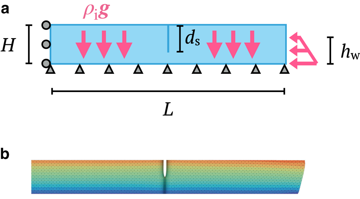
Fig. 9. (a) Loading configuration for the grounded glacier with height H = 125 m and length L = 1000 m and a no-slip boundary condition at the base. (b) Deformed configuration of the grounded glacier with a water-filled surface crevasse located at x = L/2. The purpose of this plot is to show qualitatively the deformed configuration and the crack tip opening. We, therefore, do not show the color bar for the stress contours.
We now present the net SIF versus crevasse depth curves for two different cases: dry surface crevasses and water-filled surface crevasses. In Figs. 10 and 11, we plot  $K_{\rm I}^{\rm net}$ at the crack tip for different surface crevasse depths d s while considering seawater depths h w/H = 0% and h w/H = ρ i/ρ w ≈ 90% (i.e, near-floatation) at the glacier terminus. Hydrostatic pressure is applied along the crevasse walls with hydraulic head h s/d s = 100% using a Neumann boundary condition. For both values of h w, the numerically extracted $K_{\rm I}^{\rm net}$ shows better agreement with the LEFM approach when using weight functions for the double edge cracks case rather than the single edge crack case. We also make the following observations regarding crevasse propagation and calving:
(1) the SIFs predicted by all models at the tips of dry surface crevasses are negative regardless of the seawater depth h w (see Fig. 10), which means that dry surface crevasses located far away from the terminus will not propagate in grounded glaciers frozen to the bedrock (calving does not occur);
(2) the SIFs in water-filled crevasses are positive regardless of the crevasse depth and seawater depth (see Fig. 11), which indicates that a water-filled surface crevasse can penetrate through the full depth of a grounded glacier frozen to the bedrock (calving occurs).
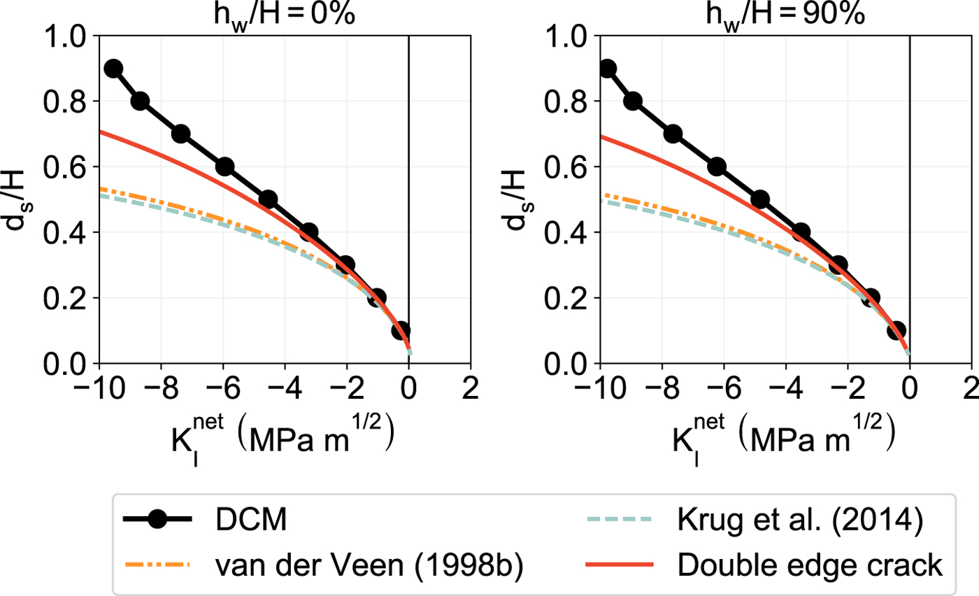
Fig. 10. Mode I net stress intensity factor  $K_{\rm I}^{\rm net}$ computed at the tip of a dry surface crevasse with depth d s penetrating through a grounded glacier with thickness H = 125 m and a no-slip boundary condition at the base.
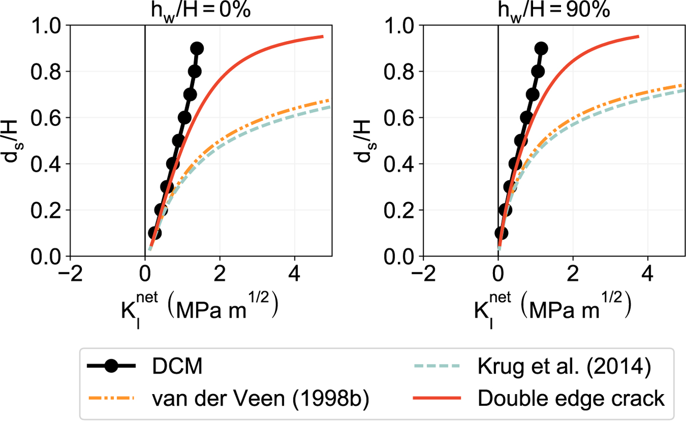
Fig. 11. Mode I net stress intensity factor  $K_{\rm I}^{\rm net}$ computed at the tip of a water-filled surface crevasse with depth d s penetrating through a grounded glacier with thickness H = 125 m and a no-slip boundary condition at the base.
The results presented thus far illustrate that the calving models using LEFM are not appropriate for grounded glaciers with a free slip or no-slip basal boundary condition because of the inappropriate assumption of weight functions in the SIF evaluation. This implies that the calving models in their present form (van der Veen, Reference van der Veen1998a, Reference van der Veenb; Krug and others, Reference Krug, Weiss, Gagliardini and Durand2014) would not be appropriate for grounded glaciers with frictional slip either.
3.3. SIF evaluation in floating ice shelves
In this section, we investigate whether the existing LEFM models are appropriate for floating ice tongues or ice shelves. For each finite element simulation, we consider an idealized, rectangular domain with length L = 4000 m and height H = 125 m under plane strain assumptions, as depicted in Figure 12. A free-slip (roller) boundary condition is applied to the left edge to prevent horizontal motion. A Robin-type boundary condition is applied to the bottom domain edge in order to simulate buoyancy of the floating ice shelf in seawater (indicated by the purple arrows in Figure 12). Hydrostatic pressure is applied as a Neumann boundary condition to the right domain edge with seawater level h w/H = ρ i/ρ w, which is the floating depth of ice. Gravity loading is applied as a body force with magnitude ρ ig, resulting in a linear variation of the horizontal Cauchy stress σ xx with depth as described in (1) in the ‘far-field’ region of the domain (i.e., sufficiently far from the terminus and the grounding line). For each simulation, we position the crevasse at x = L/2 where terminus effects vanish so that the numerically computed σ xx matches the theoretical value in (1). We compute  $K_{\rm I}^{\rm net}$ at the tip of the crevasse using each LEFM model assuming the ice shelf is a finite-thickness slab with a single edge crack (see Fig. 3a).

Fig. 12. (a) Loading configuration for the fully floating ice shelf with height H = 125 m and length L = 4000 m. (b) Deformed configuration of the fully floating ice shelf with a water-filled basal crevasse located at x = L/2. The purpose of this plot is to show qualitatively the deformed configuration and the crack tip opening. We, therefore, do not show the color bar for the stress contours.
We now present the SIF versus crevasse depth curves for three different cases: dry surface crevasses, water-filled surface and basal crevasses. In Figs. 13–15, we plot  $K_{\rm I}^{\rm net}$ at the crack tip for different surface crevasse depths d s and basal crevasse depths d b. In Figure 13, we plot $K_{\rm I}^{\rm net}$ for dry surface crevasses; and in Figs. 14 and 15 we plot $K_{\rm I}^{\rm net}$ for water-filled surface and water-filled basal crevasses, respectively. The numerically extracted $K_{\rm I}^{\rm net}$ shows good agreement with the LEFM models until the point d s/H = 60%, after which the LEFM models overestimate the SIF in comparison with the DCM. Because the net far-field longitudinal stress (i.e., away from the terminus and the grounding line) is the same for a floating ice shelf and a grounded glacier of the same thickness, the SIF versus crevasse penetration depth curves obtained from the LEFM models are the same in both cases, which is not correct. The numerically evaluated SIF versus crevasse depth curves for the floating ice shelf are indeed different from those for the grounded ice slab, owing to the difference in the basal boundary condition. We also make the following observations regarding crevasse propagation and calving:
(1) the SIFs at the tips of dry surface crevasses are negative for all depths, as shown in Figure 13, indicating that such crevasses will not propagate in a floating ice shelf (calving does not occur);
(2) the SIFs at the tips of water-filled surface and basal crevasses are positive for all depths, as shown in Figs. 14 and 15, indicating that such crevasses will propagate the entire thickness of a floating ice shelf (calving occurs);

Fig. 13. Mode I net stress intensity factor  $K_{\rm I}^{\rm net}$ computed at the tip of a dry surface crevasse with depth d s penetrating through a floating ice shelf with thickness H = 125 m. The DCM result continues to deviate from the van der Veen (Reference van der Veen1998b) and Krug and others (Reference Krug, Weiss, Gagliardini and Durand2014) result for d s/H > 0.8, however, the lines extend beyond the bounds of the plot.

Fig. 14. Mode I net stress intensity factor  $K_{\rm I}^{\rm net}$ computed at the tip of a water-filled surface crevasse with depth d s penetrating through a floating ice shelf with thickness H = 125 m. The hydrostatic pressure within the surface crevasse has a hydraulic head h s = d s (i.e., fully-filled crevasse).

Fig. 15. Mode I net stress intensity factor  $K_{\rm I}^{\rm net}$ computed at the tip of a water-filled basal crevasse with depth d b penetrating through a floating ice shelf with thickness H = 125 m. The hydrostatic pressure within the basal crevasse has a hydraulic head h w = 0.9 H.
The results presented in this section indicate that the SIFs at the tips of surface and basal crevasses in a floating ice shelf are quite different from those in grounded glaciers with free basal slip, even if the far-field longitudinal Cauchy stress σ xx is the same in both cases. The LEFM models assuming the domain as a finite-thickness ice slab with a single edge crack predict SIFs that are in good agreement with those computed from the DCM for d s/H < 60% or d b/H < 60%, but the two approaches diverge for d s/H > 60% or d b/H > 60%. Therefore, we conclude that the calving models using LEFM in their present form are not entirely appropriate for evaluating SIFs at the crevasse tips in floating ice shelves due to the assumption of a traction-free basal boundary condition. However, from an iceberg calving perspective, this discrepancy would not significantly affect the outcome (i.e., whether calving will occur) because both the analytically and numerically computed SIFs are generally much greater than the fracture toughness for ice (K Ic = 0.1 − 0.4 MPa m1/2). Consequently, the calving models presented in van der Veen (Reference van der Veen1998a,Reference van der Veenb); Krug and others (Reference Krug, Weiss, Gagliardini and Durand2014) may be consistently predicting iceberg calving from floating ice shelves, despite the discrepancy in calculating the SIF.
4. CONCLUSIONS
In this paper, we reviewed several LEFM models for finite-thickness rectangular slabs with a single edge crack, double edge cracks, and a central through the crack. We considered three calving models using LEFM from the glaciology literature (van der Veen, Reference van der Veen1998a,Reference van der Veenb; Krug and others, Reference Krug, Weiss, Gagliardini and Durand2014) and evaluated their appropriateness for evaluating the SIF at the tips of surface and basal crevasses within grounded, cantilevered, and floating ice slabs. Model-predicted SIFs were compared, against the SIF values obtained using the DCM together with finite element analysis. The results of our study reveal several important findings:
(1) The basal boundary condition (e.g., grounded with free slip at the base, cantilevered, or floating) significantly changes the SIF, even if the net longitudinal stress in the far-field (sufficiently far away from the terminus or the grounding line) is the same;
(2) The weight functions F(λ), G(λ, γ) and β(z, H, d) in the calving models using LEFM, which were originally developed assuming the ice slab to be a finite-thickness slab with a single edge crack and zero traction on the base, are not applicable to the gravity-loaded grounded glaciers with free-slip or no-slip (frozen) boundary conditions at the base, as shown in Figs. 6 – 11. The broader implication for calving criteria is that the LEFM models of van der Veen (Reference van der Veen1998a, Reference van der Veenb); Krug and others (Reference Krug, Weiss, Gagliardini and Durand2014) are appropriate only for certain cases, despite the discrepancies in SIF computation. For example, in the case where the SIF is negative, the discrepancy does not matter because the crevasse will not propagate and calving will not occur. Similarly, when the SIF is positive and greater than the fracture toughness of ice, the discrepancy does not matter because the crevasse will propagate full depth and calving occurs.
(3) The calving models using LEFM seem to be appropriate for surface and basal crevasses in floating ice shelves, however, discrepancies in model-predicted and numerically-evaluated SIFs arise for deeper crevasses (i.e., d s/H > 0.6 and d b/H > 0.6), as shown in Figs. 13–15. The broader implication for calving criteria is that the LEFM models of van der Veen (Reference van der Veen1998a, Reference van der Veenb); Krug and others (Reference Krug, Weiss, Gagliardini and Durand2014) may be appropriate for floating ice shelves, despite the discrepancies in SIF computation, for the reasons mentioned above in point 2.
The important finding of this paper is that the calving models using LEFM (van der Veen, Reference van der Veen1998a, Reference van der Veenb; Krug and others, Reference Krug, Weiss, Gagliardini and Durand2014) may be appropriate for floating ice tongues or shelves, but not for grounded glaciers. Therefore, we wish to caution ice-sheet modelers against applying these LEFM calving models to grounded glaciers and instead recommend the use of the correct weight functions provided in Appendix A. We recognize that calving models using LEFM are attractive because they can be efficiently incorporated into numerical ice-sheet models to study large-scale calving dynamics. Because the SIF evaluation in the LEFM models is largely dependent on the domain geometry and boundary conditions (i.e., single edge crack or double edge cracks), we recommend using numerical techniques for SIF evaluation within ice-sheet models for real glaciers and ice shelves with arbitrary geometries and/or boundary conditions. The DCM employed in this paper can provide a simple and accurate means of evaluating the SIF compared with other methods, such as the J-integral (Rice, Reference Rice1968) or contour integral method (Stern and others, Reference Stern, Becker and Dunham1976). Because the calculation of SIFs using the DCM can be done in a perfectly parallel manner on high-performance computing platforms, it may be a viable method for implementing calving laws based on LEFM theory into numerical ice-sheet models. However, there are a couple of technical questions relevant to iceberg calving to be addressed in future research:
(1) Knowing that ice behaves like a Maxwell viscoelastic solid on shorter timescales and like a viscous non-Newtonian fluid on longer timescales, we do not know whether LEFM theory is appropriate to model crevasse propagation within Stokes flow-based ice-sheet models. Specifically, is it appropriate to calculate SIFs in the small-deformation LEFM models with the quasi steady-state stress field obtained by solving the full Stokes equations (or their approximations) in large-deformation nonlinearly viscous ice flow models? To address this question comprehensively, we need to apply viscoelastic fracture mechanics theory and evaluate time-dependent SIFs. This can be accomplished by applying the elastic-viscoelastic correspondence principle to the associated elastic solution in the Laplace domain (Garzon, Reference Garzon2013). However, the mathematics of viscoelastic fracture mechanics can be complicated; instead, creep damage mechanics within a Stokes flow formulation may provide a computationally viable method (Jiménez and others, Reference Jiménez, Duddu and Bassis2017).
(2) Knowing that the failure of ice can be quasi-brittle in nature, we do not know whether LEFM theory is appropriate to model crevasse propagation in glaciers and ice sheets at very low strain rates. Specifically, is the fracture process zone at the tip of a crevasse sufficiently smaller than the crevasse length for LEFM theory to be valid? An approximate estimate of the fracture process zone size is given by (Hillerborg and others, Reference Hillerborg, Modéer and Petersson1976)
(15)If we assume Poisson's ratio ν = 0.35, fracture toughness K Ic = 0.1 − 0.4 MPa m1/2 (van der Veen, Reference van der Veen1998a) and critical stress under uniaxial tension σ c = 0.01–0.2 MPa (Pralong and Funk, Reference Pralong and Funk2005; Krug and others, Reference Krug, Weiss, Gagliardini and Durand2014), then l c ≈ 0.2–1400 m for glacier ice. The estimated range of l c indicates the large uncertainty in the size of the fracture process zone and the limitation of applying LEFM theory to crevasse propagation. Therefore, to address this question, a comprehensive validation of LEFM models against observational data on calving from real glaciers is necessary. Mottram and Benn (Reference Mottram and Benn2009) have tested crevasse depth models using a field study at Breiðamerkurjökull, Iceland, but remarked that measuring crevasse depths accurately is difficult, dangerous and time-consuming. $$l_{\rm c} \approx {K_{\rm Ic}^2(1-\nu^2) \over \sigma_{\rm c}^2}. $$

Additionally, simulating crevasse propagation using LEFM theory is sensitive to the location and size of pre-existing crevasses and is computationally cumbersome because it requires geometry update or re-meshing, as discussed in Yu and others (Reference Yu, Rignot, Morlighem and Seroussi2017). To overcome the modeling and numerical issues associated with the LEFM approach, we support the development of the creep damage mechanics approach in conjunction with Stokes flow formulations (Jiménez and others, Reference Jiménez, Duddu and Bassis2017) to study crevasse propagation and calving. Although the damage mechanics approach is computationally more expensive than the LEFM approaches, it can be implemented in a feasible manner in depth-integrated shallow shelf formulations (Keller and Hutter, Reference Keller and Hutter2014).
ACKNOWLEDGMENTS
We gratefully acknowledge the funding support provided by the National Science Foundation's Office of Polar Programs via grants #PLR-1341428. We thank Prof. Jeremy Bassis for the helpful discussion on calving models and Prof. Armando Duarte for his insights on the numerical evaluation of stress intensity factor. We also thank scientific editor Ralf Greve and two reviewers, Arne Keller and an anonymous reviewer, for valuable comments that helped improve the manuscript.
APPENDIX A
The weight function m C(z, H, d) for the finite-thickness slab with a central through the crack is given as (Tada and others, Reference Tada, Paris and Irwin1973, Reference Tada, Paris and Irwin2000),
 $$m_{\rm C}(z, H, d) = {2 \over \sqrt{2H}} \left\{ 1 + 0.297\sqrt{1 - \left({z \over d} \right)^2} \right. $$
 $$\quad\quad\quad\quad \times \left. \left[ 1 - \cos \left( {\pi d \over 2 H} \right) \right] \right\} \phi \left({d \over H}, {z \over d}\right), $$
where z is the coordinate along the length of the crack, H is half of the slab thickness (see Fig. 3b-c), and d is the crack length. The function ϕ is given by,
 $$\phi \left({d \over H}, {z \over d}\right) = {\sqrt{\tan \left({\pi d\over 2H} \right)} \over \sqrt{1 - \left({\cos \left({\pi d \over 2 H}\right)}{\big /}{\cos \left({\pi z \over 2 H} \right)}\right)^2}}. $$
Similarly, the weight function m D(z, H, d) for the finite-thickness slab with double edge cracks is given as (Tada and others, Reference Tada, Paris and Irwin1973, Reference Tada, Paris and Irwin2000),
 $$m_{\rm D}(z, H, d) = {2 \over \sqrt{2H}} \left[ 1 + f_1 \left({z \over d} \right) f_2 \left( {d \over H} \right) \right] \phi \left({d \over H}, {z \over d}\right), $$
where the function f 1 is given as,
 $$f_1 \left( {z \over d} \right) = 0.3 \left[1 - \left({z\over d} \right)^{5/4} \right], $$
and the function f 2 is given as,
 $$f_2 \left( {d \over H} \right) = {1 \over 2} \left[1 - \sin \left( {\pi d \over 2H} \right) \right]\left[2 + \sin \left( {\pi d \over 2H} \right) \right]. $$
The weight functions m C(z, H, d) and m D(z, H, d) may be substituted in place of the term m(z, t, d) in (5) to compute the stress intensity factor at the tip of a crack with length d. For either weight function, (5) must be integrated from the base of the crack (z = 0) to the crack tip (z = d).
APPENDIX B
The weight functions F(λ) used and G(λ, γ) utilized by the van der Veen (Reference van der Veen1998a, Reference van der Veenb) LEFM models are given by,
 $$\eqalign{F(\lambda) & = 1.12 - 0.23 \lambda + 10.55 \lambda^2 - 21.72 \lambda^3 \cr & \quad + 30.39 \lambda^4,}$$
and
 $$\eqalign{G(\lambda, \gamma) & = \left[{3.52(1-\gamma) \over (1-\lambda)^{3/2}} \right] - \left[{4.35 - 5.28\gamma \over (1 - \lambda)^{1/2}} \right] \cr & \quad + \left[ {1.3 - 0.3 \gamma^{3/2} \over (1 - \gamma^2)^{1/2}} + 0.83 - 1.76 \gamma \right] \left[ 1 - (1-\gamma) \lambda \right]},$$
where the terms λ = d s/H and γ = z′/H; and z′ = H − z is the vertical coordinate measured from the top of the domain.
APPENDIX C
The weight function β utilized in the Krug and others (Reference Krug, Weiss, Gagliardini and Durand2014) LEFM model is given by,
 $$\eqalign{\beta(y,H,d) &= {2 \over \sqrt{2\pi(d-y)}} \Bigg[ 1 + M_1 \left(1 - {y \over d}\right)^{1/2} \cr & \quad + M_2 \left(1 - {y \over d} \right) + M_3 \left(1 - {y \over d} \right)^{3/2} \Bigg].}$$
where y is the vertical coordinate, H is the domain height, and d is the crevasse height. For surface crevasses, y = z′ = H − z and d = d s. For basal crevasses, y=z and d = d b. The constants M 1, M 2, and M 3 are given by polynomial functions that account for the geometry of the ice slab,
 $$\eqalign{M_1 &= 0.0719768 - 1.513476 \lambda - 61.1001 \lambda^2 \cr &\quad + 1554.95 \lambda^3 - 14583.8 \lambda^4 + 71590.7 \lambda^5 \cr &\quad - 20\,5384 \lambda^6 + 35\,6469 \lambda^7 - 36\,8270 \lambda^8 \cr & \quad + 20\,8233 \lambda^9 - 4\,9544 \lambda^{10},}$$
 $$\eqalign{M_2 &= 0.246984 + 6.47583 \lambda + 176.456 \lambda^2 \cr &\quad - 4058.76 \lambda^3 + 37303.8 \lambda^4 - 18\,1755 \lambda^5 \cr & \quad + 52\,0551 \lambda^6 - 90\,4370 \lambda^7 + 93\,6863 \lambda^8 \cr &\quad - 53\,1940 \lambda^9 + 12\,7291 \lambda^{10},}$$
 $$\eqalign{M_3 &= 0.529659 - 22.3235 \lambda + 532.074 \lambda^2 \cr &\quad - 5479.53 \lambda^3 + 28592.2 \lambda^4 - 81388.6 \lambda^5 \cr & \quad + 12\,8746 \lambda^6 - 10\,6246 \lambda^7 + 35780.7 \lambda^8,}$$
where the term λ = d/H.


 Open access