
1 INTRODUCTION
The story of the language known in former Yugoslavia as Serbo-Croatian is a telling example of the complex interaction between linguistic microvariation and its political environment. This story has been told many times from many different points of view and no version is likely to be accepted by all interested parties. In fact, the protagonists of this story are not only Croats and Serbs living in Croatia and Serbia respectively, but a whole range of ethnic groups living on the territory of four present-day countries and former Yugoslav republics, Bosnia-Herzegovina, Croatia, Montenegro, and Serbia, whose official standard languages now carry the respective country names: Bosnian, Croatian, Montenegrin, and Serbian (BCMS).
The questions of the unity of the language and its name(s)—Is it a single language with multiple names, or multiple languages each with a single name?—have spurred long and passionate debates often leading to absurd political decisions and social phenomena. A good example of the current linguistic paradox appears in what is supposed to be a relatively straightforward description of the population of a state: the distribution of mother tongues in Montenegro’s 2011 census (number of speakers in parentheses):Footnote 1 Montenegrin (229,251), Serbian (265,895), Bosnian (33,077), Albanian (32,671), Croatian (2,791), Montenegrin-Serbian (369), English (185), Croatian-Serbian (224), Bosniak (3,662), Hungarian (225), Macedonian (529), Mother tongue (3,318), German (129), Roma (5,169), Romanian (101), Russian (1,026), Slovenian (107), Serbo-Croat (12,559), Serbo-Montenegrin (618), Other (2,917), Regional languages (458), Does not want to declare (24,748).
Taking the census entries literally, one would think that more than 20 distinct languages are spoken in a population of the size of around 620,000. A reader a little more familiar with the linguistic practices in the country could say that 10 of these entries (in bold), covering around 90% of the population, are just different names for the same linguistic entity. The latter interpretation, however, would be a crude simplification of the linguistic reality, neglecting the very fact recorded in the census, namely the need for different names. Linguistic grouping remains poorly understood in all four former Yugoslav republics, playing at the same time an important role in political moves.
The separation of the former Yugoslav republics into independent states during the wars in the 1990s only revived linguistic debates, which had been going on since the first steps towards unifying South Slavic groups in the early 19th century. Throughout this time, the focus has been on prescribing (through grammars, dictionaries, and orthographic manuals) and imposing (through regulatory acts) a particular set of words or writing rules on a particular territory. Linguists, writers, and other scholars have taken part in the debate by publishing opinionated articles, signing written agreements and declarations.Footnote 2 All these publications aim at defining how the language should be used, with less interest in understanding how it is used in reality.
In contrast to its perceived political importance, regional linguistic variation on the territory of BCMS is not systematically monitored. The most recent comprehensive overview of the dialectal variation is Pavle Ivić’s handbook published in 1956. Subsequent dialectological studies have resulted in numerous individual descriptions of rural idioms, but no broad-coverage surveys have been conducted. Beside a small number of “ideal” dialectological informants,Footnote 3 little is known on how people on the territory of BCMS actually speak.
Until recently, urban varieties were not considered an interesting research topic, under the assumption that they conform to the standard language prescribed in official grammars and dictionaries or otherwise are not valuable. Changes in communication technology leading to a democratization of public communication allowed more variation in language use to be observed in public spaces. This contributed to a raised awareness of regional variation beyond the traditional dialectological framework. The language of blogs, comments, and posts tends to be highly varied, including both regional and social variation. Moreover, a lot of this language use is recorded and accessible for research. This situation creates a new opportunity for an objective, broad-coverage study of the delicate issue of linguistic practices in BCMS.
The goal of our study is to measure empirically the most commonly cited regional differences between Bosnian, Croatian, Montenegrin and Serbian using large data sets available through user-generated content on the Internet. We aim to establish spatial spreads of the categories in question and the degree to which they follow the current borders between the four countries. A potential agreement between linguistic and administrative boundaries can be expected given some traditional differences and considering that the four countries have been conducting independent standardizations since the split of the former Yugoslavia. However, the opposite can be expected based on what is known about the history of language use in this region: while administrative borders changed often, at no point in time did they coincide with linguistic boundaries. Our analysis is intended to provide empirical evidence that can serve in picturing the current state of language use. It is highly automated, which means that the procedure can be repeated at regular time points in the future with relatively low costs. In this way, we can monitor directly historical changes in the spatial distribution of linguistic features to see whether and how importantly changes in political conditions contribute to deepening the divide between successors to a once common standard language.
We limit our study to the language used on the social network Twitter, a typical modern means of communication that allows non-professionals to express publicly their own observations, comments, or opinions. Twitter is especially interesting for studying regional variation because it allows geo-localization of the posts. The language of Twitter is usually considered to be highly non-standard. However, we expect to see an impact, to a significant degree, of language standardization, since recent work (Fišer, Erjavec, Ljubešić & Miličević Reference Fišer, Erjavec, Ljubešić and Miličević2015) has shown that as much as 90% of Twitter content follows the linguistic norms. Speakers who create this content are mostly sensitive to the effects of language standardization: they are typically educated and in constant contact with public communication. With the lack of comprehensive linguistic surveys, the language on Twitter is currently the closest approximation of the real language used in everyday life in the territory of BCMS.
2 RELATED WORK
Most of our study falls within the domain of modern dialectology. The difference between traditional and modern dialectology has been underlined by several researchers who gradually introduced new goals and methods in the study of regional linguistic variation (Chambers & Trudgill, Reference Chambers and Trudgill1998; Britain, Reference Britain2002).
Traditional dialectology, instantiated in the study by Ivić (Reference Ivić1956) mentioned above, tracks phonetic (different pronunciation of the same word known to vary) and lexical (different terms used to express the same content) variation. Its goals changed over time from the 19th-century focus on reconstructing the history of a language to the 20th-century efforts to pin down the borders between dialects and to preserve non-standard varieties that are disappearing under the pressure of standardization.
Modern dialectology, often overlapping with sociolinguistics, is concerned with the full range of regional variation including urban varieties and, especially, social diversification. Introduction of social factors in the study of linguistic variation is often attributed to Labov (Reference Labov1963), who showed that the variation in centralized vs. open pronunciation of an English diphthong has a “social meaning”: it distinguishes the native inhabitants of an island (Martha’s Vineyard) from visitors. Sociolinguistics has since become a wide field, with only part of it focusing on social factors in relation to regional variation, mainly following the goals set by Trudgill (Reference Trudgill1974). Our study continues this strand, whose central topics are dialect levelling and formation of new varieties (Hornsby, Reference Hornsby2009; Trudgill, Gordon, Lewis & MacLagan, Reference Trudgill, Gordon, Lewis and MacLagan2000). The difference between our and previous studies is that we do not address multiple social factors that might be involved in linguistic variation and potential change in our target region. We focus instead on one feature: the recent emergence of state borders that cut across the territory of a single dialect.
A setting similar to the one that we study is addressed by Woolhiser (Reference Woolhiser2005), who analyzes the effects of the state border between Poland and Belarus, established for the first time after World War II and dividing a Belarusian dialect into two countries. Woolhiser identifies a number of features that show divergent developments on the two sides of the border. The variant on the Belarusian side tends to converge with the standard Belarusian and Russian, while the variant of the dialect on the Polish side moves away from both the Belarusian version of the dialect and standard Polish. While we ask questions similar to those asked by Woolhiser (Reference Woolhiser2005), the context of the potential linguistic change is quite different. First, the standard “roof” languages in our case are not as easily identifiable as in the case of Polish and Belarussian (as explained in more detail below). Second, the data that we analyze cannot be taken as representing a dialect as opposed to a standard language. As mentioned above, the language of Twitter is more likely to be situated somewhere between these two points of Woolhiser’s “vertical” variation axis. Finally, while Woolhiser (Reference Woolhiser2005) discusses in depth the prevalence of just a few features on a few locations, our analysis involves relatively large datasets from many locations collected and analyzed automatically.
Automatic quantitative analysis is what our study has in common with dialectometry, a line of research that is considered a part of modern dialectology, where methods are proposed to measure linguistic distance between language varieties. The first quantification of linguistic distance was proposed by Séguy (Reference Séguy1971), who counts the number of lexical items that are shared by two varieties and compares this measure with geographical distance. Linguistic distance measures are subsequently refined to take into account various facts about the distributions of linguistic features. Goebl (Reference Goebl1982, Reference Goebl1984) introduces feature weights as a function of their frequency to take into account the fact that some features are more spread across varieties and therefore not indicative of the similarity of any particular pair. Similarity at the word level is taken into account by Nerbonne, Heeringa, van den Hout, van der Kooi, Otten & van de Viset (Reference Nerbonne, Heeringa, Erik van den Hout, van der Kooi, Otten and van de Vis1995) and Nerbonne, Heeringa & Kleiweg (Reference Nerbonne, Heeringa and Kleiweg1999) using string edit distance. While dialectometry is traditionally focused on spatial variation, Wieling, Nerbonne & Baayen (Reference Wieling, Nerbonne and Baayen2011) propose an integrative analysis where social and regional factors of variation are included in a single (mixed-effects) model which predicts the distance of a number of Dutch dialects from the standard language. All these studies rely on data sets collected in traditional dialectological surveys. These sets, as mentioned above, contain lexical and phonetic realizations of selected words known to vary. While we employ some of the techniques elaborated in dialectometry, our data set includes a wider range of features, including morphology and syntax.
An important novelty in modern dialectology is the interest in a wider structural range, including morpho-syntax (Bart, Glaser, Sibler & Weibel, Reference Bart, Glaser, Sibler and Weibel2013; Glaser, Reference Glaser2013; Szmrecsanyi, Reference Szmrecsanyi2008), discourse, and pragmatics (Pichler & Hessen, Reference Pichler and Hesson2016). As speakers’ intuitions about formal or high-level phenomena are not easily captured with traditional questionnaires, extending the scope of research was only possible thanks to new methods of data collection.
Language corpora represent a new data source suitable for studying a wider variety of features. Introduction of corpus data into the study of regional variation (Speelman, Grondelaers & Geeraerts, Reference Speelman, Grondelaers and Geeraerts2003; Kortman & Wagner, Reference Kortmann and Wagner2005; Szmrecsanyi, Reference Szmrecsanyi2008) allows collecting information about text frequency of the varying forms and constructions as they are spontaneously produced. The main disadvantages of this data source are uneven spatial coverage (naturally occurring texts tend to be more concentrated in particular regions) and sparseness of linguistic phenomena.Footnote 4 Our collection of Twitter messages can be considered a corpus consisting of micro-texts. It allows studying various phenomena related to language use. Unlike corpora employed in previous studies, which are collected by experts, our texts are automatically harvested from a social network.
Data from social networks have already been used to study linguistic variation in relation to social and geographical factors, mostly in the field of computational linguistics. Here we focus on the work involving Twitter. This network has become a popular data source for computational experiments thanks to its application programming interface (API), which allows automatic collection of many messages and user metadata for research purposes.
Unlike previously reviewed work, which is primarily concerned with the varied forms of semantically equivalent items, the research on Twitter includes content analysis (enabled by the fact that Twitter is essentially text). Eisenstein, O’Connor, Smith & Xing (Reference Eisenstein, O’Connor, Smith and Xing2010,Reference Eisenstein, O’Connor, Smith and Xing) propose a hierarchical model that learns (with moderate success) to associate a particular topic with a particular geographic region. Most of the subsequent studies look for significant associations between textual features and demographic characteristics of the speakers (Eisenstein, Smith & Xing, Reference Eisenstein, Smith and Xing2011; Nguyen, Smith & Rosé, Reference Nguyen, Smith and Rosé2011), but several studies address geographical factors. Doyle (Reference Doyle2014) shows that the spatial distribution of linguistic features extracted from Twitter corresponds to the distributions previously established with traditional dialectological methods. Eisenstein, O’Connor, Smith & Xing (Reference Eisenstein, O’Connor, Smith and Xing2014) model the spatial diffusion of new linguistic features in time, showing that it is strongly influenced by demographic factors. In these studies, uneven spatial distribution and data sparsity are addressed with sophisticated statistical models involving latent variables and various transformations of initial counts. Our analysis is primarily exploratory (and not inferential), but we employ sampling and smoothing techniques to abstract from initial observations and identify patterns in regional variation.
Twitter language studies outside of (American) English are rather rare. Gonçalves & Sánchez (Reference Gonçalves and Sánchez2014) try to cluster worldwide Spanish varieties regionally, but they find a predominant urban vs. rural divide. Scheffler, Gontrum, Wegel & Wendler (Reference Scheffler, Gontrum, Wegel and Wendler2014) attempt to assign German tweets to one of the given regions by calculating regional probability of words, but without taking into account potential topic variation. Our work builds upon previous studies on automatic discrimination between BCMS in newspaper texts (Ljubešić, Mikelić & Boras, Reference Ljubešić, Mikelić and Boras2007), as well as Twitter data (Ljubešić & Kranjčić, Reference Ljubešić and Kranjčić2015). Previous work has shown that good discrimination can be obtained for practical purposes; we apply automatic analysis to address specific questions of interest to the general study of language use and change.
3 LANGUAGE CONVERGENCE AND DIVERGENCE IN BCMS
The current linguistic situation on the territory of BCMS is a result of linguistic, political, and cultural developments that have interacted in complex ways throughout history. A comprehensive account of these developments is Alexander’s (Reference Alexander2013) chapter on language and identity in BCMS. Alexander (Reference Alexander2013) shows that today’s situation is not substantially different from any other historical period since the beginning of the 19th century and the first attempts at creating strategic language policies in the region. These attempts were well embedded in general tendencies throughout 19th-century Europe, when most of the currently known national states were established. Language standardization was an integral part of creating national identities.
Creation of a standard language usually involves: 1) choosing a single (predominant or prestigious) linguistic variety to be imposed on a clearly delimited territory; 2) codifying the chosen variety with official grammars and dictionaries; 3) imposing the codified variety through the state administration. Political power—and not only in BCMS—is often expressed in terms of language standardization.
Linguistic standardization in BCMS took place in a political context where none of the main cultural centers, Belgrade (Serbia), Zagreb (Croatia), Sarajevo (Bosnia-Herzegovina), or Cetinje (Montenegro),Footnote 5 had the political power to fully implement it. The territory was split between two big empires, Austro-Hungarian and Ottoman, with different degrees of autonomy exercised by the Slavic population on the territory of today’s BCMS. Montenegro and Serbia were the first to obtain full independence in 1878, but not with the same borders as today. In this context, the choice of the variety to be standardized in the cultural centers was strongly influenced by the romantic vision of a common future of all Slavic groups living in a single independent Slavic state. However, this vision was not strong enough to fully overtake more local, regional traditions, that insisted on cultural and, especially, religious differences. This interplay between two opposite interests of all involved parties—integration and separation—remained constant until the present day.
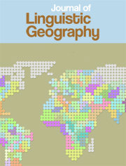
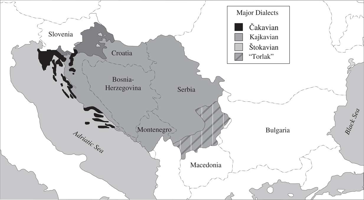
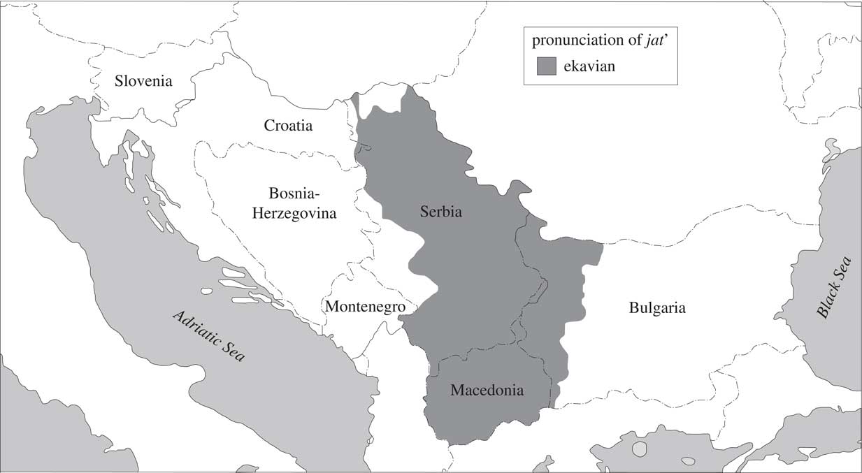
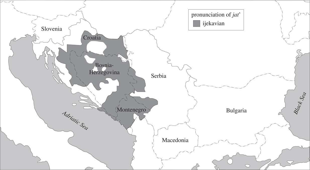
Regional linguistic varieties in BCMS are best identified by the values of two prominent features: 1) the form of the question word what, and 2) the phonetic reflex of the Proto-Slavic vowel jat’. The value of the first feature, clustering with a number of others, gives the most distinctive varieties, which can be labelled as ‘što’, ‘kaj’, and ‘ča’. The spatial distribution of these varieties, which constitute separate dialects, if not languages, is plotted in Map 1, taken from Alexander (Reference Alexander2013:346). Variation with respect to the second feature gives more nuanced, but still prominent varieties ‘e’, ‘je’, ‘i’. Its spatial distribution is also plotted in Maps 2–4, taken from Alexander (Reference Alexander2013:350–352).
Map 1 Čakavian, kajkavian and štokavian dialects.
Map 2 Area of ekavian pronunciation.
Map 3 Area of ijekavian pronunciation.
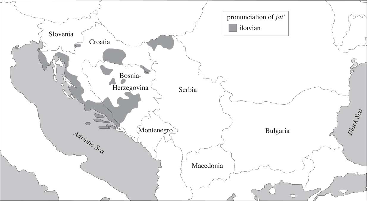
Map 4 Area of ikavian pronunciation.
As can be seen in the maps, spatial distributions of the two features are rather different. The ‘ča’ variety mostly has ‘i’ for the other feature, and ‘kaj’ has ‘e’. The most widely spread ‘što’ variety can have all three values for the other feature. Note also that these different feature values were already characteristic of the vernaculars spoken in the territory of today’s BCMS in the 19th century. Their geographical placement has not changed since, but the domain of their use has shrunk in those varieties that did not become part of the standard in the meantime.
We can see all these varieties as possible choices for the future standard language in the period immediately preceding the standardization efforts. The options to choose from in the four cultural-administrative centers are summarized as follows:
∙ Belgrade: ‘što + e’ or ‘što + je’. The first option was (and still is) predominant on its territory, but the second one was also used, especially in folk tales and poems, highly valued at the time. The second option also allowed a connection with the Serbian-oriented (Orthodox) population outside the territory under the influence of Belgrade.Footnote 6
∙ Zagreb: ‘kaj + e’ or ‘ča +i’ or ‘što + je’. There was no clear preference for any of the three options. The first one was (and still is) spoken in the city of Zagreb and had a literary tradition. The second one also had a rich literary tradition and prestige, mostly in Dalmatia. The third one was (and still is) most widely spread in the Croatian-oriented (Catholic) population.
∙ Sarajevo: ‘što + je’ was the only option.
∙ Cetinje: ‘što + je’ was the only option.
It is clear from this summary that the best choice for a common language was ‘što + je’. This is precisely the option that was proposed by Vuk Karadžić, the prominent Serbian language reformer supported by the Austrian authorities. His proposal was accepted in Zagreb, the center of the Illyrian movement which had the goal of unifying all South Slavs and countering the dominance of German and Hungarian language in that area. The proposal was accepted just partly in Belgrade, where the Vukovian reform was eventually accepted in everything except that the ‘što + e’ version was kept. The adoption of the ‘Vukovian’ proposal meant that almost the same variety was codified in all four centers. This provided the basis for further unification efforts, especially during the time of Yugoslavia, whose main official language became Serbo-Croatian (or Croato-Serbian).
Unification tendencies are, however, just one half of the story. Throughout this time, almost equally strong were the opposite tendencies that called for keeping local varieties and connections with the literary tradition. This was especially the case in Zagreb, where unification required the biggest effort due to the existence of the Štokavian, but also Kajkavian and Čakavian literary traditions, and where unification was seen as Serbian predominance. Divergences were codified through two “variants” in the 1960s, an “eastern” (Belgrade) and a “western” (Zagreb) one, and by constitutionally allowing separate “standard idioms” in the four Serbo-Croatian speaking republics in 1974. After the breakup of Yugoslavia, the separationist position became predominant in all four centers.Footnote 7 Despite the desire on the part of all concerned to separate the four standards as much as possible, all four centers still have “almost the same” variety as a base, the one that was chosen for codification in the 19th century. This variety is now being re-codified in four different directions to mark the political breakup.
Our study addresses the effects which the above processes have had on everyday language use in contemporary BCMS.
4 DATA EXTRACTION
4.1 Dataset
The data for our study were collected with TweetCat (Ljubešić, Fišer & Erjavec, Reference Ljubešić, Fišer and Erjavec2014), a tool for harvesting Twitter data in low-density languages, i.e., languages infrequently occurring in the Twitter stream. The collection method uses the Twitter Search API and high frequency words specific to the language(s) of interest, searching for authors who use these words, and performing language identification on the whole language production of each candidate user. All candidate users who pass the language identification filter are added to the user index and their tweet production is collected. Both the user identification and the user data collection procedures are run iteratively for as long as required. In our collection method we defined a single list of high-frequency words and therefore ran a single process for collecting the data. This process was run from June 2013 up to the end of 2016.
Throughout this collection period we gathered data from 70,107 users who in turn produced 38,726,488 tweets. For the purposes of this study, we only kept the data geo-encoded in the four countries of interest (Bosnia, Croatia, Montenegro, Serbia). This restriction left us with 17,172 users and 1,755,525 tweets, i.e., 4.5% of the initial data points. After extracting the 16 variables of interest, we removed all data points (tweets) that contained no value for any of our variables, and therefore no relevant data. Our final dataset thereby consists of 13,102 users and 693,111 tweets, meaning that our 16 variables are present in 40% of geo-encoded tweets.
There is a well-known phenomenon in social media that a small number of users, often automated processes (also called bots), post the majority of content. Before moving forward, we checked our user distribution for such phenomena and found that they were not present. Our most prominent user has 1,526 published tweets, i.e., 0.22% of the entire dataset, publishing on average one tweet per day. The second and third most prominent users account for 0.18% tweets, the fourth, fifth and sixth 0.16% tweets, etc., showing that our user-dependent distribution does not have a dominating head and that there is no need for discarding or even underrepresenting the most prominent users.
An early analysis of our dataset already confirmed our assumption that the Twitter usage across the four countries of interest varies greatly. In Table 1 we present the distribution of tweets, reporting the number of tweets from each country, as well as the percentage of tweets covered by that country. We also compare the distribution of tweets with the distribution of country areas. The numbers show that three countries are underrepresented given their area, while one (Serbia) is vastly overrepresented, accounting for 81% of Twitter content, but only 39% of territory. For this reason, we used our full dataset while performing country-conditioned calculations, whereas for calculations that are not performed on specific countries, but on the area in general, we worked with a sampled dataset in which the distribution of tweets by country follows the country area distribution. We constructed the sampled dataset by randomly drawing from our initial dataset. In that sampled dataset the percentage of tweets follows the percentage of the area of a country, both percentages for Serbia, for instance, being 39%.
Table 1 Distribution of tweets by country, compared to the area distribution by country, and the sampled dataset following the area country distribution.

4.2 Variables of Interest
We look at 16 two-level categorical variables, summarized in Table 2. Variable names, levels and examples are provided, as well as their raw and relative frequencies. The frequencies were calculated on the sampled dataset, in order to overcome the danger of over-quantifying variables more frequently occurring in Serbia and vice versa.
Table 2 A summary of variables whose spatial distribution was studied.
As can be seen from the table, the variables belong to three levels of linguistic structure: phonetics, lexis, and morphosyntax. They were selected from a larger set of candidates based on the criteria of linguistic relevance, ease of automatic retrieval, and sufficient coverage in the data.
Linguistic relevance was determined through a literature review. Variables mentioned in a number of works were considered, including traditional grammars and orthography manuals (for Serbian: Pešikan, Jerković & Pižurica, Reference Pešikan, Jerković and Pižurica2010; Stanojčić & Popović, Reference Stanojčić and Popović2008; Stevanović, Reference Stevanović1989; for Croatian: Barić, Lončarić, Malić, Pavešić, Peti, Zečević & Znika, Reference Barić, Lončarić, Malic, Pavešić, Peti, Zečević and Znika1997; for Bosnian: Halilović, Reference Halilović2004; Jahić, Halilović & Palić, Reference Jahić, Halilović and Palić2000; for Montenegrin: Čirgić, Pranjković & Silić, Reference Čirgić, Pranjković and Silić2010,Reference Eisenstein, O’Connor, Smith and Xing; Perović, Silić & Vasiljeva, Reference Perović, Silić and Vasiljeva2009), as well as studies explicitly dealing with differences between the new standard languages (cited below, with reference to individual variables).Footnote 8 Expectedly, most works deal with Serbian and Croatian, and their mutual differences. Tošović (Reference Tošović2008) conducted an extensive overview of reference works for the four languages and found that, out of 289 resources consulted, 57% were descriptions of Serbian, 41% descriptions of Croatian, 2.8% descriptions of Bosnian, and only 0.1% descriptions of Montenegrin. The studies dealing with differences were initially also heavily focused on Serbian and Croatian, but Bosnian has subsequently received a lot of attention, largely due to attempts to disentangle its Croatian-like and Serbian-like features. The youngest of the standard languages, Montenegrin, is, as expected, the least covered one. Note also that the available studies mostly target the standard as described in reference works, with little empirical data about actual language use.
We focus on variables that can be automatically identified based on the surface form of words, and/or the entries in the available morphological lexicons (hrLex and srLexFootnote 9 ; Ljubešić, Klubička, Agić & Jazbec, Reference Ljubešić, Klubička, Agić and Jazbec2016).Footnote 10 We exclude those variables that are difficult or impossible to retrieve in an automatic manner, something which is often due to homonymy; for instance, the contrast between te (characteristic of Croatian) and pa (more typical of Serbian), both meaning ‘then’, was not studied due to te also being the accusative singular 2nd person personal pronoun (as in vidim te ‘I see you’), as well as the feminine nominative/accusative form of a demonstrative pronoun (as in te kuće ‘those houses’).
The variables also had to be frequent enough to provide a meaningful number of data points for the analysis of spatial distribution. One of the main consequences of this constraint meant that under lexical variables we only look at function words, despite the differences in the inventory of lexical words being typically listed as the most prominent ones (see e.g. Brown & Alt, Reference Browne and Alt2004:7; Piper, Reference Piper2009:549-550; Tošović, Reference Tošović2008:183).Footnote 11 It should also be mentioned that it was impossible to reach a sufficient number of variables with similar frequencies; the implications of the large differences in frequency will be discussed when necessary in the results section.
In what follows, we provide more detailed descriptions of individual variables and the procedures used in their extraction.
e:je
The e:je variable concerns one of the features central to defining the dialects on the territory of BCMS—the Proto-Slavic vowel jat’ and its different contemporary reflexes (described in more detail in Section 3). We look at e (as in mleko ‘milk’, or pesma ‘song’) and (i)je (mlijeko, pjesma). The e reflex is characteristic of Serbia, while (i)je is found in Croatia, Bosnia-Herzegovina and Montenegro. Based on reference descriptions, this is the variable whose geographical distribution is expected to be most straightforward.Footnote 12 It is at the same time the most frequent variable we look at.
The e:je variable was extracted using a lexicon file containing the list of target items in one column, and variable values in another (as illustrated by the examples in Table 3; see also Ljubešić, Samardžić & Derungs, Reference Ljubešić, Samardžić and Derungs2016). The list was automatically generated from the inflectional morphological lexicons hrLex and srLex (Ljubešić et al., Reference Ljubešić, Samardžić and Derungs2016) by searching for pairs of words in which both had the same morphosyntactic description and identical word forms except for the transformations (ije vs. e or je vs. e), and both had just one possible canonical form (lemma). A total of 146,864 word forms were listed.
Table 3 A sample of the feature extraction lexicon used for e:je.

rdrop
In some words in BCMS, e.g., jučer/juče ‘yesterday’, the final r can either occur or be dropped; the former option is more typical of Croatian, and the latter of Serbian (see frequencies in Tošović, Reference Tošović2009). The specific words we look at are juče(r) ‘yesterday’, prekjuče(r) ‘day before yesterday’, veče(r) ‘evening’, naveče(r) ‘in the evening’, uveče(r) ‘in the evening’, predveče(r) ‘in the early evening’, and takođe(r) ‘also’.
This variable was also extracted through a lexicon file. The file was created manually; it only included the words listed above, and for each of them the value with regard to r drop.
k:h
The k:h alternation is another systematic phonetic phenomenon often cited as a differential marker between Croatian and Serbian. It occurs at word beginning in words of Greek origin which started with ch-, so in contemporary BCMS we find word pairs such as kemija/hemija ‘chemistry’, or kirurg/hirurg ‘surgeon’ (more examples in Silić, 2008). K is consistently used in Croatian, and h in Serbian. At the level of the norm, Bosnian and Montenegrin pattern with Serbian and use h (Halilović Reference Halilović2004:48; Perović et al., Reference Perović, Silić and Vasiljeva2009); however, k seems to also be possible in Bosnia-Herzegovina, as will be shown in our later analyses.
The k:h variable was extracted using a manually created lexicon file. All inflected forms of each relevant lemma were included, for a total of 587 word forms. The lemmas were identified through the lists reported in the literature and through dictionary searches.
h:noh
The last of our phonetic variables is related to the presence/absence of h, which is sometimes omitted at word beginning, and omitted or replaced with an alternative (typically j or v) within a word. Examples of pairs with(out) an initial h drop are hrđa/rđa ‘rust’ and hrvanje/rvanje ‘wrestling’. In non-initial positions, snaha/snaja ‘sister/daughter-in-law’, čahura / čaura ‘cocoon; capsule’, and gluh/gluv ‘deaf’ exemplify the contrast.
The problem of where h is to be written and pronounced dates back to the 19th century, when a general rule was developed stating that it should be used where it was required by etymological criteria; this rule was kept in the orthographic norm of Serbo-Croatian, but it was differentially adopted in the different variants, with Serbian mostly allowing both forms, and Croatian and Bosnian keeping the h (Čedić, Reference Čedić2001).Footnote 13 The presence of h is particularly characteristic of Bosnian, where it is added in some words that do not contain it in Croatian and did not necessarily contain it etymologically—kahva ‘coffee’ (Croatian kava, Serbian kafa), lahko ‘easily’ (Croatian and Serbian lako), and similar. These forms were non-standard in Serbo-Croatian, but they entered the norm for Bosnian later on (Halilović, Reference Halilović2004:22-23). The Bosnian norm also banned the possibility of using suv ‘dry’, duvan ‘tobacco’, and other similar Serbo-Croatian forms allowed alongside suh and duhan. Montenegrin seems to pattern with Serbian, but without a clearly formulated rule, and with some inconsistencies—the orthography manual lists only snaha, only gluv, and both čaura and čahura (Perović et al., Reference Perović, Silić and Vasiljeva2009).
The lexicon of words relevant for the h:noh variable was compiled manually, taking into account all inflected forms; a total of 1088 word forms were included. Note that the forms that are highly specific of Bosnian were omitted, as they do not belong to the etymological pattern the normative rules were based on, and sometimes also have multiple equivalents in the other standards (cf. kahva / kava / kafa).
sto:sta
Our first lexical variable has to do with the feature behind the first major division in BCMS. In the dialects based on što (as opposed to kaj and ča), the standard form of the interrogative pronoun ‘what’ is što in Croatian, Bosnian and Montenegrin, and šta in Serbian (both šta and što are listed in the reference works, but šta is more common). Tošović (Reference Tošović2009) reports corpus frequencies that show što (including its other uses, as a relative pronoun and as a short form for zašto ‘why’) to be 10-20 times more frequent than šta in Bosnian and Croatian; in Serbian, šta is about 4 times more frequent than što (which is also used as a relative pronoun and a short form for zašto).
In terms of automatic extraction, this variable is very simple in one sense, as it is based on a very short lexicon file, but not so straightforward in another, due to the presence of a diacritic sign. We included in the lexicon file the forms što and šta. We were not able to follow the general approach of disregarding diacritics in the analysis—that is taking sto and sta into account—due to homonymy of sto, meaning ‘table’ and ‘one hundred’.
dali:jeli
In BCMS, yes/no questions are asked using interrogative particles je li and da li. Je li is the norm in Croatian, where da li only occurs in the colloquial register (Hudeček & Vukojević, Reference Hudeček and Vukojevic2007). Serbian uses both forms, but je li is commonly shortened to je l’, jel’ or jel and used colloquially, while the preferred full form is da li. Bosnian seems to be mixed, with a moderate preference for Croatian-type question forms (see Špago-Ćumurija, 2009). The Montenegrin orthography manual lists both je li and da li (Perović et al., Reference Perović, Silić and Vasiljeva2009).
As a multi-word variable, dali:jeli was extracted using regular expressions, ‘\bda li\b’ and ‘\bje li\b’ respectively. The shorter alternatives (je l’, jel’, jel) were not included, as they could not be treated as a separate variable level (recall that we focus on two-level variables) and merging them with the more formal je li would bias the results.
s:sa
The preposition s(a) ‘with’ is another point of divergence in BCMS. In standard Croatian, the choice between the forms s and sa is based on phonetic factors—sa is to be used before s, š, z, ž (sa šlagom ‘with cream’), before consonant clusters such as ks or ps (sa Ksenijom ‘with Ksenija’), and before the instrumental form of the 1st singular pronoun ja (sa mnom ‘with me’); s should be used in all other cases (s ledom ‘with ice’, s Ivanom ‘with Ivan’). In standard Serbian, there is a rule about using sa before similar-sounding consonants, and about using s in fixed expressions such as s jedne strane ‘on the one hand’, but the choice is explicitly left to the speakers in all other cases.Footnote 14 Tošović (Reference Tošović2009) reports the relevant frequencies in the parallel corpus GRALIS, showing that s is around four times more frequent than sa in Croatian and around twice as frequent in Bosnian, while in Serbian sa is around 2.5 times more frequent than s.
In terms of extraction, s:sa was one of the simplest variables, obtained using a two-form manual lexicon file.
mnogo:puno
The intensifying adverbs mnogo and puno ‘many, a lot’, are both used in all variants of BCMS, but puno is particularly typical of Croatian, and mnogo of Serbian. The use of puno in Serbian is the subject of numerous discussions, and some normativists have long been trying to ban it, claiming that its only meaning is that of an adverb derived from the adjective pun ‘full’. For this reason, it is often perceived as colloquial.
This variable was also extracted through a two-form manually created lexicon file.
ko:tko
The interrogative pronoun meaning ‘who’ takes the form ko in Serbian, Bosnian, and Montenegrin, and tko in Croatian; the same goes for the derived pronouns neko/netko ‘somebody’, niko/nitko ‘nobody’, svako/svatko ‘everybody’, and iko/itko ‘anybody’. Tko is the older form, and some authors use its survival in Croatian as an argument for its greater conservativeness compared to Serbian (see Pranjković, 1997). We focus on the derived forms and leave out the actual tko and ko, due to ko also being used as a very frequent short form of kao ‘like, as’. Ne(t)ko and sva(t)ko are excluded as well, due to also being neuter singular forms of the demonstratives neki ‘some’ and svaki ‘every’, leaving in the analysis ni(t)ko ‘nobody’ and i(t)ko ‘anybody’.
This variable was also obtained using a manual lexicon. Only nominative forms were listed, as t is absent in the other cases for both tko and ko type pronouns, which would bias the results.
long:shortinf
The full infinitival form of verbs in BCMS ends in either - ti or - ći (pisati ‘write’; ići ‘go’). In Croatian, it is quite common to shorten the infinitives by removing the final i (as in pisat, ić), sometimes because of the rule for future formation (for verbs ending in -ti, e.g., pisat ću ‘I will write’; more detail below, under the synth:nonsynth variable), and sometimes colloquially (see Miličević & Ljubešić, Reference Miličević and Ljubešić2016; Miličević, Ljubešić & Fišer, Reference Miličević, Ljubešić and Fišer2017); this phenomenon is virtually non-existent in Serbian.
The extraction of infinitives was based on a lexicon file derived from hrLex and srLex, from which all infinitives were obtained based on the morphosyntactic descriptions. The short forms were defined by taking away the final - i.
da:inf
One of the features most often cited as differentiating between the syntax of Serbian and Croatian is the composition of complex predicates containing modal (moći ‘can’, morati ‘must’, smeti ‘dare, may’, trebati ‘need’) or phasal verbs (početi ‘begin’, završiti ‘end’), which in Serbian tend to take as complement da (‘that’) + present tense form of the verb, a construction typical of the Balkan Sprachbund (as in volim da pišem ‘I like to write’), while in Croatian, infinitives are used when the subject remains the same (volim pisati) (Kovačić, Reference Kovačić2005; Piper, Reference Piper2009; Tošović, Reference Tošović2008). In Bosnian, the two constructions are normatively equal (Čedić, Reference Čedić2001).
We extracted this variable using a list of verb infinitives and present tense forms from the hrLex and srLex morphological lexicons.
synth:nonsynth
The future tense has a synthetic form for most verbs in Serbian, with clitic forms of the auxiliary hteti ‘want’ merged with the verb (as in pisaću ‘I will write’), while the analytic form is used in Croatian, with the infinitive (short form) and the auxiliary as separate words (pisat ću); the analytic form is used in Serbian too when the verb ends in - ći (reći ću ‘I will say’). This variable is very frequently mentioned in discussions of the relationship between Serbian and Croatian (see Bekavac, Seljan & Simeon, Reference Bekavac, Seljan and Simeon2008; Kovačić, Reference Kovačić2005; Piper, Reference Piper2009; Tošović, Reference Tošović2008). Bosnian uses both kinds of forms, and there does not seem to be a very clear preference for one or the other (for conflicting views in the literature see Bekavac et al., Reference Bekavac, Seljan and Simeon2008; Silić, Reference Silić2008; Špago-Ćumurija, 2009). The Montenegrin norm allows both types of future formation, underlining that synthetic forms are more common (Perović et al., Reference Perović, Silić and Vasiljeva2009).
Again, as with previous morphosyntactic variables, the extraction process was based on the hrLex and srLex lexicons, the latter containing synthetic future forms.
adjg
In adjectival inflection in BCMS it is sometimes possible to append a vowel at the end of a word for easier pronunciation and/or stylistic markedness. The most typical case is - a in genitive singular forms of masculine adjectives; e.g., novoga ‘of the new’ is fairly frequently used in standard Croatian instead of novog, more typical of Serbian.
This variable was obtained again by exploiting the hrLex and srLex morphological lexicons.
ira:isa:ova
This variable concerns the morphological composition of verbs. When deriving borrowings from international verbs, Croatian typically uses the verbal suffix - ira (as in promovirati ‘promote’, registrirati ‘register’), while - isa and - ova prevail in Serbian (promovisati, registrovati). As far as Bosnian is concerned, Čedić (Reference Čedić2001) mentions that in the past two decades - ira verbs have become more frequent than - isa and - ova verbs, but that it also happens that an - ira infinitive and an inflected form belonging to the - ova paradigm appear in the same text (e.g., organizirati plus organizuju instead of organiziraju).
To extract this variable, a similar procedure was followed as for e:je, with the difference that canonical forms rather than word forms were matched for everything but the ira vs. isa/ova suffix. From the identified canonical forms, lexicons of all word forms were produced.
treba
In standard Serbian, the modal verb trebati ‘need’ is often used impersonally. This is the result of a prescriptive tradition that bans constructions such as trebam da idem ‘I need.1SG to go.PRES.1SG’ and requires treba da idem ‘I need.3SG to go.PRES.1SG’. No such rule is instantiated in the grammar of Croatian, where personal forms are normally accompanied by infinitives, as in trebam ići ‘I need.1SG go.INF’. Interestingly, this difference is not commonly listed in the works dealing with the differences between Croatian and Serbian.
The variable treba was extracted using the regular expressions ‘\btreba(m|s|mo|te|ju)\b|\btreba(?! da)’, covering present tense forms of the verb (without the adjacent da), and ‘\btreba da\b’, for the impersonal form of the verb.
ica:ka
Our last variable concerns the suffixes used for deriving feminine agent nouns, which partly overlap, and partly differ across BCMS. The suffix -ica (as in nastavnica ‘teacher’) is present in all languages, but it is dominant only in Croatian and Bosnian, while in Serbian the suffixes -ka (čitateljka ‘reader’) and -inja (laborantkinja ‘lab technician’) are very frequent as well (Dražić & Vojinović, Reference Dražić and Vojinović2009; Šehović, Reference Šehović2009). The choice of the suffix also depends on the ending of the masculine noun from which the feminine form is derived—inter-varietal differences between - ica and - ka mostly occur after - or and - ar (as in profesor – profesorica / profesorka ‘professor’, or zubar – zubarica / zubarka ‘dentist’). For the purposes of this paper, we thus only looked at - rica and -rka, as both - ica and -ka are too generic as word endings and do not always mark agents.Footnote 15
The variable was extracted by identifying feminine noun lemmata in the hrLex and srLex lexicons that end in the corresponding suffix pairs. The extracted list was additionally checked by hand.
Given that the variables were extracted automatically, and some of them could only be approximated, some noise in the data was inevitable. This is very often due to diacritic omissions, which are fairly common on Twitter, and which we disregarded (e.g., noc was treated equally as noć ‘night’). This approach led to some atypical cases of homonymy. Such cases were sometimes easily predictable, and we adjusted the procedure to avoid them, as for the sto:sta variable. However, unpredictable overlaps also occurred. The frequent ones (whether related to diacritic omissions or not) were spotted during the analysis; e.g., the form braće, which can be the future tense of the verb brati ‘pick (fruits, flowers, etc.)’, but is much more often the genitive plural of the noun brat ‘brother’—in the final analysis of the future forms we disregarded such cases, keeping only those for which no match with other lemmas in the lexicon were found. Some less frequent overlaps were discovered only later and were deemed infrequent enough not to have a major impact on the results; e.g., the string glasace was classified as a synthetic future form (glasaće ‘he/she/it/they will vote’), even though in some contexts in the data it actually means glasače ‘voters.ACC’).
Note also that for most variables the situation is not expected to be black and white as to the geographical distribution of levels, given that both values are often attested within the same standard languages. What we are more likely to witness is a dominance of one level in some areas, and the other level in another, possibly corresponding to the patterns prescribed or described as characteristic in normative works. This is understandable given the shared recent history, and the literature does often say the current differences are more often a matter of frequency of use and/or stylistic value, than complete divergence (see e.g. Piper, Reference Piper2009:543; Tošović, Reference Tošović2009).
5 ANALYSES
We performed two main types of analyses: a) estimating the spatial distribution of the set of variables described above, and b) computing linguistic distance between the four administrative regions (BCMS) given the described variables and the current state borders. In the first case, we looked for linguistic boundaries irrespective of administrative borders, and once the linguistic boundaries were identified, we compared them to administrative borders. In the second case, we measured linguistic similarity given the state territory. The second analysis contains a measure of similarity between the states and a measure of internal consistency in the choice of specific variable levels within one state. In this way, we measured both inter- and intrastate similarity. We refer to interstate similarity as distance (directly inverse similarity) and to the intrasimilarity as a country’s variable consistency.
We performed all calculations in the statistical software R,Footnote 16 mostly exploiting existing packages, but defining functions ourselves when necessary.
5.1 Estimating Spatial Distributions
The goal of the spatial analysis is to establish which level of a variable is dominant on which territory, regardless of the known state borders. We smoothed and extrapolated the originally observed counts using kernel density estimation (KDE), a well-established method for representing point observations as density surfaces. We show the areas of dominance on a map and call those visualizations level dominance plots. We performed this calculation for each of our 16 variables and compared its output manually with the BCMS state borders.
The local value of a density surface corresponds to the number of observations of the respective feature level proximate to this location. A kernel function is applied for smoothing the signal, and thus account for local noise. After computing density surfaces for each feature level individually, local intensities are compared and only the level with maximum local intensity is preserved and mapped as the dominant level. Hence, the level dominance plot function visually represents linguistic areas dominated by individual feature levels.
It is important to note that KDE distributes the probability of a variable level over a unit area under the curve. The probability of a variable level in one area is thus relative to its probability in other areas. An extremely high probability of a level in one observation region leaves little probability to be assigned to this level in other areas. This is an important shortcoming of KDE in the case of uneven spatial distribution of observations. If there is a high-density area for one level, but no such area exists for the other level, the dominance of the level for which there is a high-density area will be systematically underestimated in all the areas outside of the high-density area. To give one example, the long infinitive form is overall more frequent than the short form and its dominance should spread over most of the territory of BCMS. However, calculating KDE on the initial observations would show a different spread, more concentrated on a smaller region (Serbia in this case). This would happen because the territory of Serbia includes a high-density area (the city of Belgrade), where the longer form is dominant. The extremely high density of the predominant longer form in this area would leave little probability to be assigned to the long form in other regions. Since there is no such high-density point for the short form, its probability will be more evenly distributed across regions and thus estimated by KDE as higher than the probability of the long form in many regions where this is, in fact, not true.
To address this issue, we performed KDE on balanced samples. We randomly selected observations so that the number of observations used for KDE is proportional to the territory of each of the four countries. By doing this, we simulate a more even distribution of observations, making our data set more suitable for KDE.
The same feature of KDE that is inconvenient in dealing with uneven spatial distribution of observations becomes crucial for eliminating the general frequency bias in cases where one variable level is generally much more frequent than the other. Transforming the original counts into a probability distribution with per-level normalization allows us to detect the variation in the differences between levels across regions. Without this transformation the more frequent levels would be perceived as dominant on the whole territory.
5.2 Computing Linguistic Distance
We continue our analyses by focusing on the differences in distributions of our variables in the four countries. We perform these analyses on the full dataset as disproportional amounts of data available in different countries does not impact the per-country distributions that we base our analyses on. In these analyses, we primarily exploit the information-theoretic measure of Jensen-Shannon divergence (JSD), which quantifies the information loss occurring if we assume one distribution over another.
We calculated two basic types of distance: distance between variables and distance between countries. The distance between variables tells us how similar the chosen linguistic features are to one another, and also whether some features tend to cluster together. High feature clustering is indicative of distinct varieties. The distance between countries provides an aggregate score of how much the language used in the four countries differs.
When calculating the distance between two countries, we calculate for each variable JSD between the two country distributions, obtaining thereby 16 distances which we average. To give an example, when calculating the distance between Bosnia-Herzegovina and Croatia, we calculated JSD over their distributions for the e:je variable, as well as for the 15 remaining variables, finally averaging over the 16 obtained distances.
For calculating the distance between two variables, we used the same initial variable distributions as when calculating the distance between two countries, but grouped them now not by variable, but by country. To obtain a single distance we again averaged the JSDs obtained on each distribution pair, the pairs now coming from different variables in identical countries. To give a similar example to the previous one, for calculating the distance between the e:je and ica:ka variables, we calculated JSD over the Bosnian distributions of these two variables, repeating the procedure on the three remaining countries.Footnote 17 Finally, we calculated the average of the four obtained distances.
Finally, to quantify the consistency of each country with regard to our 16 variables of interest, we used an index calculated as the average of the lower ratios of all the variables. The two extremes of this metric are 0.0 if in each of the variables one level covers the whole distribution, and 0.5 if each of the variables has an equiprobable distribution, therefore both levels of a variable having the probability of 0.5.
6 RESULTS
6.1 Estimating Spatial Distributions
Given that Twitter is known to be used more in densely populated areas, while analyzing the level dominance plots, we take into account the amount of data available from specific regions. Namely, some of the regions are known to be sparsely populated, therefore a level dominance in these areas can be due to generalization over small amounts or even no data. We represent the amount of data available in Map 5 in the form of a heatmap. As expected, the map shows the largest cities in the area to be the centers of content production. The only area completely lacking Twitter data is the Dinarides area on the border between Croatia and Bosnia-Herzegovina, known to be largely unpopulated. While most of Serbia is well covered with data, Croatia seems to have the least consistent coverage, with large areas in the northeast and the central part showing very scarce data coverage. A similar, but less drastic situation can be observed in southwestern Bosnia-Herzegovina and in border areas between Bosnia-Herzegovina and Montenegro, and Montenegro and Serbia.
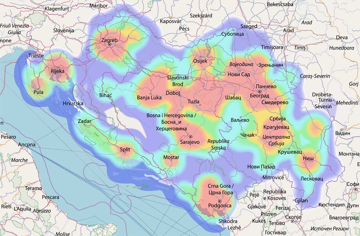
Map 5 Heatmap representing the spatial distribution of data points in our sampled dataset.
To simplify the presentation of the level dominance plots of each of the 16 variables, we organize them into four basic groups given the state patterns they follow:
1. Croatia vs. remaining countries
2. Croatia and Bosnia-Herzegovina vs. Montenegro and Serbia
3. Serbia vs. remaining countries
4. No visible state pattern
An overview of the variables in the four state patterns is given in Table 4 (with color-coded variable types). The table shows that for most of our variables of choice, more precisely for three-fourths of them, a strict state pattern can be observed. There does not seem to be any correspondence between variable types and state patterns; no pattern contains only a single variable type. The most productive pattern, covering half of our variables, is the west vs. east, i.e., Croatia, Bosnia-Herzegovina vs. Montenegro, Serbia pattern. The least productive, at least in terms of the number of variables, is the Serbia vs. remaining countries pattern, although it covers the overall most frequent phenomenon, the jat’ reflex. One should notice that all patterns actually follow a relaxed west vs. east pattern, in which Bosnia-Herzegovina and Montenegro incline either to the east or to the west.
Table 4 Overview of variables given the state pattern they are grouped in. Type of variable is encoded with colour.

Map 6 depicts the level dominance plots following the Croatia vs. remaining countries pattern. While the ira:isa:ova and ko:tko variables follow the pattern in full, especially if we take into account the complex shape of Croatia, while the variables k:h and rdrop show a deviation in southern Bosnia-Herzegovina, predominantly using the Croatian-preferred level. This does not come as a surprise, given the large Croatian population living in this area.
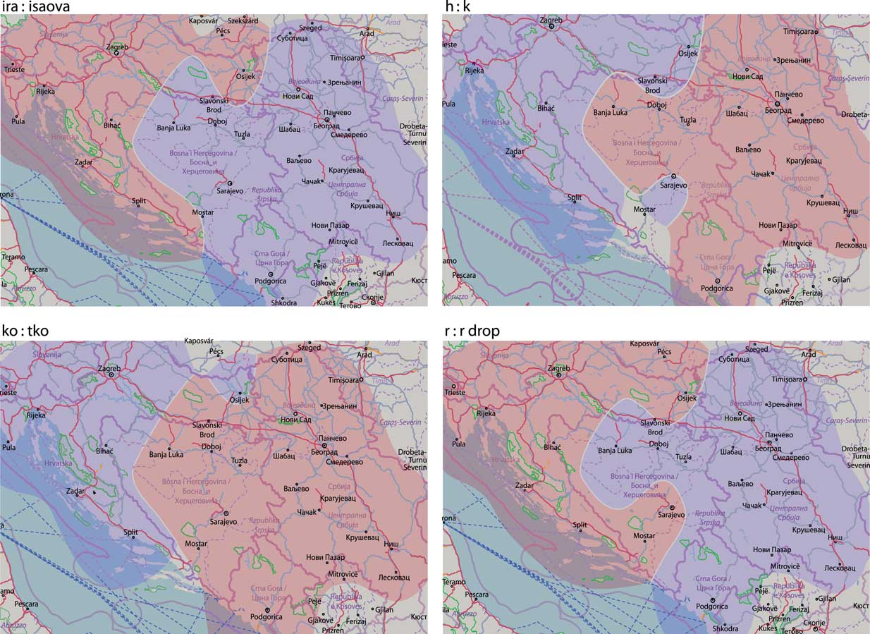
Map 6 Level dominance plots grouped in the Croatia vs. remaining countries pattern.
In Map 7, the dominance plots following the second, Croatia, Bosnia-Herzegovina vs. Montenegro, Serbia, state pattern are given. Similarly to the previous pattern, the variables da:inf, mnogo:puno and treba follow the pattern in full, while h:noh, synth: nonsynth and s:sa show a deviation, this time in the area of central-northern Bosnia-Herzegovina mostly populated by ethnic Serbs, which follows the eastern-preferred levels.
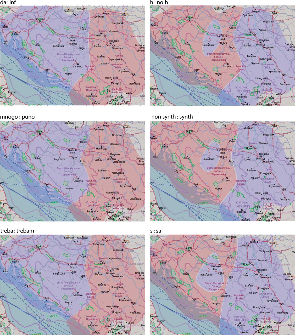
Map 7 Level dominance plots grouped in the Croatia, Bosnia-Herzegovina vs. Montenegro, Serbia pattern.
Map 8 depicts the dominance plots that follow the Serbia vs. remaining countries state pattern, namely the e:je variable and the ica:ka variable. The latter variable lacks coverage in southern Croatia, where the level dominant in the remainder of Croatia and the neighboring countries can be expected.
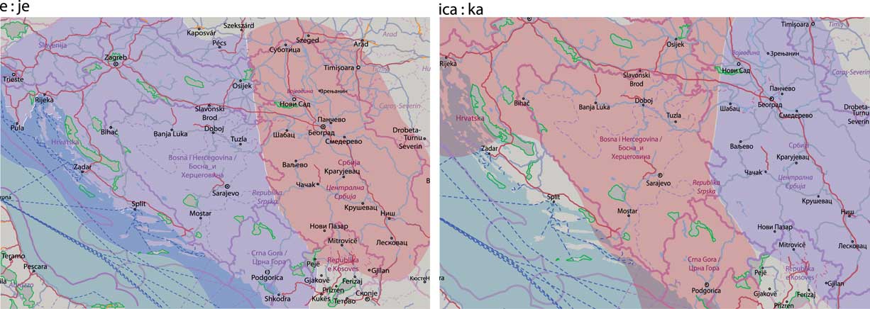
Map 8 Level dominance plots grouped in the Serbia vs. remaining countries pattern.
Finally, Map 9 contains the dominance plots showing no or partial state patterns. While dali:jeli and long:shortinf very roughly follow the Serbia vs. remaining countries pattern, the sto:sta and adjg variables show signs of a pattern not observed in the previous variables: Croatia and Montenegro leaning on one, Bosnia-Herzegovina and Serbia on the other side.
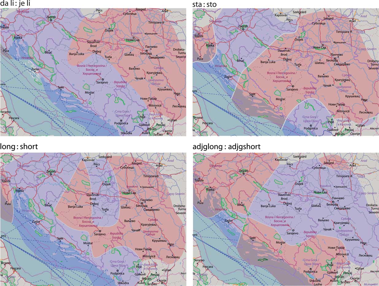
Map 9 Level dominance plots grouped in the no state pattern.
There are three main conclusions we can draw from the presented results. The first one is that most variables follow state borders, reflecting long-standing linguistic and normative differences, as well as the recent separate standardization processes. The second conclusion is that there is an overall east vs. west pattern in which Bosnia-Herzegovina and Montenegro tend to incline either to the east or to the west. The final conclusion relaxes the first one as a significant number of variables, more precisely five, break the state pattern in Bosnia-Herzegovina, with parts heavily populated either with ethnic Croats or Serbs leaning towards the level dominant in the respective “mother country.”
6.2 Computing Linguistic Distance
In Figure 1 we show the distributions of each variable in each country, grouped by variables. These distributions are the basis for the calculations whose results are given in the remainder of this section.
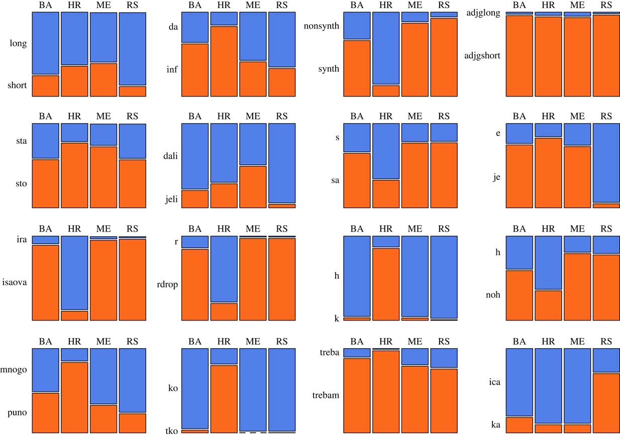
Figure 1 Per-country distribution plot of the 16 variables taken under consideration for Bosnia (BA), Croatia (HR), Montenegro (ME) and Serbia (RS).
We start from the variable distance matrix, which we represent in the form of a dendrogram (Figure 2). Our goal is to compare this border-obeying clustering of features with the results of dominance plot groupings performed in the previous section. Note that the setting of the two analyses is very different. While the previous analysis used country borders as possible explanations for the obtained dominance plots, which did not have access to border information, in this analysis these borders are our starting point by calculating per-country variable distributions. The primary goal of the comparison of the two analyses is to either challenge or further strengthen our previous conclusions.
The first cluster in the dendrogram, containing the variables k:h, ko:tko, ira:isa:ova and rdrop, fully corresponds to the pattern Croatia vs. remaining countries from the previous section. The second cluster from the left, comprising the synth:nonsynth, mnogo:puno, s:sa and h:noh variables, covers four out of six variables clustered previously in the Croatia, Bosnia-Herzegovina vs. Montenegro, Serbia pattern. The large cluster present in the right side of the figure corresponds to a smaller extent to the previously observed state patterns. The Serbia vs. remaining countries pattern, comprising the e:je and ica:ka variables, can be identified as a separate cluster, long:shortinf and dali:jeli similarly forming a cluster and being part of the no state pattern. The remaining two clusters (adjg and treba, da:inf and sto:sta) do not correspond to previously identified patterns.
We can conclude that this first analysis strongly backs our previous conclusions that dominance plots follow specific state patterns. Namely, three-fourths of the variables that are clustered together in this analysis were previously grouped into the same state patterns, and in the case of one-half of the variables, large clusters of four variables fully correspond to previously constructed state patterns.
We next analyze the calculated country distance matrix. The distances between countries are based on our 16 variables and we should stress right here that these distances do not take into account the natural frequency of occurrence of the phenomena operationalized in these variables. The country distance matrix is presented in Table 5.
Table 5 Country distance matrix calculated as average JSD.

The distance matrix shows that the most similar country pair is Bosnia-Herzegovina and Montenegro, followed by Bosnia-Herzegovina and Serbia, and Montenegro and Serbia. The least similar countries are Croatia and Serbia. These distances again follow our observations from the previous section, Croatia and Serbia presenting two extremes, and Bosnia-Herzegovina and Montenegro falling somewhere in between, but being overall closer to Serbia than to Croatia. However, as already stated, these distances are based on 16 variables that have very different frequencies of occurrence. Calculating the distance between the same languages on running text would primarily rely on the four most frequent variables that cover 81% of variable occurrences, namely e:je (Serbia vs. remaining countries), da:inf (Croatia and Bosnia vs. Montenegro and Serbia), long:shortinf (partially Serbia vs. remaining countries) and s:sa (Croatia and Bosnia vs. Montenegro and Serbia). These four variables draw Bosnia-Herzegovina much closer to Croatia, leaving Montenegro still closer to Serbia, which matches the results seen in the automatic classification of Twitter users presented in Ljubešić & Kranjčić (Reference Ljubešić and Kranjčić2015), where most of the errors come from confusing Bosnian and Croatian users on one side and Serbian and Montenegrin users on the other.
The previously presented country distance matrix can be transformed in a single-country table by averaging all the distances of a country to the remaining countries, thereby quantifying the overall distance of a country to its neighbors, i.e., its linguistic distinctness. These average distances are the following: for Bosnia it is 0.060, for Croatia 0.167, for Montenegro 0.075, and for Serbia 0.106. The results reveal Croatia to be most distant and therefore, most distinct linguistically (at least regarding the 16 chosen variables). Croatia is followed, but not closely, by Serbia, with Montenegro and Bosnia-Herzegovina being the two least distinct countries.
We wrap up this series of analyses by quantifying the variable consistency index of each country. The quantifications are the following: for Bosnia it is 0.23, for Croatia 0.18, for Montenegro 0.19, while for Serbia it is 0.14. These findings show Serbia to be the most consistent country given our variables, which can be explained by the fact that it is more compact dialect-wise than Croatia, and more centralized standard-wise than Bosnia-Herzegovina and Montenegro. Croatia and Montenegro are very close to each other and take the middle ground, while Bosnia-Herzegovina, as expected, is linguistically the most diverse country by far, in all likelihood because of the competing influences of Croatia and Serbia.
This series of analyses has once again shown that Croatia and Serbia represent linguistic extremes among our four countries of interest. Bosnia-Herzegovina and Montenegro seem to be closer to Serbia in our per-variable setting. The most linguistically distinct country is Croatia (most distant from the other countries), and the most consistent country regarding our 16 variables is Serbia.
7 DISCUSSION
The goal of our study was to empirically measure the spread of some of the features considered indicative of regional differences in BCMS, looking in particular at the extent to which this spread corresponds to the current state borders. Historical developments, including the recent separation of former Yugoslavia, give rise to opposing expectations: a match between linguistic and administrative borders can be interpreted as an effect of rather constant divergent norming tendencies, emphasized by the most recent political split; no match can be interpreted as an effect of equally constant unifying trends and a common dialectal basis of the standard languages.
Although our analysis does not provide a simple answer, we can draw several generalizations regarding the regional distribution of a set of features, and we can show how these features constitute differences between the language used in the four countries.
At the most general level, Croatian and Serbian represent two extremes, while Montenegrin and especially Bosnian fall in between them, changing sides depending on the variable; overall, Montenegro leans more frequently to Serbia, and Bosnia-Herzegovina to Croatia. However, when each language is contrasted to the other three languages, Croatian is more distinct from the rest than Serbian; along similar lines, Bosnian and Montenegrin are overall closer to Serbian than to Croatian. The country that most frequently does not correspond to variable level boundaries is Bosnia-Herzegovina, depicting the ethnic heterogeneity of the population, and the strong role of language as a differentiating factor.
Our findings reflect quite closely the recent history of the languages in question. Since the first 19th century attempts at joint standardization, Croatia and Serbia have always constituted two opposed poles of the shared standard, each with its own historical baggage and its own agenda—Serbia more focused on the unifying potential of a common literary language in the Yugoslav context, and Croatia intent on preserving at least some of its diversity and its distinctive features in a situation that it perceived as Serbian dominance.Footnote 18 The language spoken in Montenegro was seen as a variant of Serbian and, until Montenegro gained independence, it was largely absent from the disputes. Bosnia-Herzegovina, on the other hand, had the advantage that its majority native speech fully corresponded to the chosen standard, but it also had to keep focus on maintaining a fragile balance among its different ethnic and religious groups (Croats, Serbs and Muslims), siding with Croatian on some language features, with Serbian on others, and enriching its lexical base with words of Turkish origin. As our data show, these tendencies are especially distinguishable today.
As far as different linguistic features are concerned, the feature that certainly carries the most linguistic relevance is our e:je variable, on which Serbia is distinct from the remainder of the countries in prevalently using e forms such as mleko ‘milk’ rather than (i)je forms (mlijeko). This feature reflects a prominent dialectal distinction that played an important role in establishing a standard diasystem instead of a single standard already in the 19th century. Regarding the other features, we observe a considerable degree of bundling, but we do not find plausible linguistic explanations for the clusters of features.
Divergent language norming, from the 1960s “variants” and the 1970s “standard idioms” to more recent separate standardizations, seems to have brought the desired divergent results for some features (e.g., the synthetic and analytic forms of the future tense, a point of much dispute within the wider question of phonetic vs. etymological spelling), but not so clearly for others (note in particular the widespread use of da li in Croatia). Features that are felt as being more related to what sounds natural than to strict normative rules also lead to clear patterns in some cases. For example, the fairly high incidence of short infinitives in Montenegro can be related to the properties of a major dialect; even more prominently, the - ka suffix in Serbian is one of its distinguishing features despite not being emphasized in prescriptive rules. Again, it is difficult to draw a conclusion applying to most features of the same type.
When it comes to the results concerning the internal variable consistency of the four countries, the situation is somewhat surprising at first sight. While the Croatian norm is usually described as being purist and strict, and the Serbian one as allowing multiple options and more free choice based on the speakers’ intuitions, for our sample of variables the country that is most consistent in its choices of variable values is actually Serbia. Croatia and Montenegro are less stable, with Bosnia-Herzegovina, expectedly, being the most varied from this point of view too.
A possible explanation is again essentially a historical-linguistic one, having to do with the fact that standardization required different levels of adaptation in different countries. The native speech of Serbia’s cultural centers was not only closer to the proposed standard compared to the native speech of Croatia’s center, but Serbia was overall more centralized and more unified in terms of the vernacular even before standardization—the speech of Belgrade and Novi Sad had clear prestige, which it still does. The diversity of Croatia’s dialects with their rich literary tradition meant that strict rules were needed if a common base was to be created. However, strict rules did not eliminate the regional variation, which continues to show up in everyday speech.
8 CONCLUDING REMARKS
Overall, we can conclude that in BCMS linguistic boundaries do, to some extent, match administrative boundaries, as well as ethnic divides in Bosnia-Herzegovina. However, the match is never complete, and boundaries differ for different variables. The dominant boundary establishes a west vs. east divide, where Croatia and Serbia are fairly stable on their respective ends, while Bosnia-Herzegovina and Montenegro align sometimes with one, and sometimes with the other.
Of course, the results that we obtained depend heavily on the specific variables we selected and should ideally be expanded by including additional variables. However, given that we focused on some of the core features brought up in almost all works dealing with differences within BCMS, our findings can be seen as empirical evidence that should not be ignored in further linguistic accounts of the linguistic situation in BCMS. In future work, we will study more variables, looking more closely at the distinction between rules grounded in actual language use and the purely normative ones, as well as apply approaches where variables are not defined in advance, but where the full amount of linguistic signal is processed in search for the most distinguishing features of that signal.
Finally, our results seem to lend support to the view of Twitter as a new source of data for deriving spatial distributions of linguistic features. Given a medium level adoption of Twitter in most of the countries, we can expect other, more popular social media, primarily Facebook, to be an even better source of linguistically relevant spatial signal.
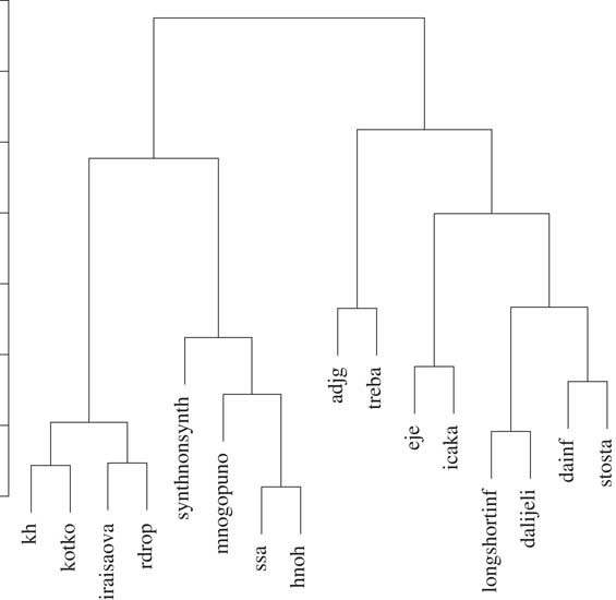
Figure 2 Dendrogram based on the variable distances calculated via average JSD.
Acknowledgments
The work presented here is partially funded by the SNSF grant 160501 and by a special grant awarded by the UZH URPP ‘Language and Space.’


