
1 Motivation
Commonly in linguistic geography, important questions are associated with the distribution, relations and changes of linguistic phenomena in space and time. In dialectology, in order to understand the processes behind spatiotemporal patterns of dialect evolution and area formation, researchers traditionally investigated the distribution patterns of individual linguistic phenomena in search of overlaps and correspondences in space. Such research often involved drawing boundaries between the usage areas of dialectal variants that corresponded to a certain survey question in a dialectal survey. Two conceptualizations describe these spatial transitions and boundaries. The concept of isoglosses idealizes sharp boundaries between the usage areas of dialectal variants. The concept of dialect continua implies that since dialect areas cannot be sharply delimited due to individual variables (i.e., the survey question) following different patterns of regional variation (e.g., Chambers & Trudgill, Reference Chambers and Trudgill2004), gradual transitions ought to be expected between dominance areas of variants for individual variables as well (cf., Bach, Reference Bach1950:58–62; Fischer, Reference Fischer1895:80–81, as referred to in Pickl, Reference Pickl2013b). There is an agreement in variationist linguistics today (e.g. Girnth, Reference Girnth2010:112-116; Pickl, Reference Pickl2013; Wieling & Nerbonne, Reference Wieling and Nerbonne2015) that spatial distributions are usually not as sharply delimited as isoglosses drawn on maps would suggest (Haag, Reference Haag1898; Maurer, Reference Maurer1942; Viereck, Reference Viereck1986); thus continua are present. Nevertheless, dialectology still discusses both concepts of dialectal interfaces in parallel, without a clear concept resolving the different types of transitions (Chambers & Trudgill, Reference Chambers and Trudgill2004:105). The presence of vague definitions of spatial boundaries in areal linguistics points toward a research gap worth investigating from a more geographic perspective, using methods of the spatial sciences. Since linguistic boundaries are in essence conceptualized as transitions of varying steepness, ranging from the abrupt changes assumed by isoglosses to the more gentle transitions represented in dialect continua, we propose quantitative modeling of linguistic boundaries and transitions between dialectal variants as gradients.
Most dialectal variants have an only vaguely defined dominance zone which, instead of sharp boundaries, more or less gradually transitions into the dominance zone of another variant (cf., Chambers & Trudgill, Reference Chambers and Trudgill2004; Heeringa & Nerbonne, Reference Heeringa and Nerbonne2001; Kessler, Reference Kessler1995; Pickl & Rumpf, Reference Pickl and Rumpf2012). Despite the continuing interest in boundaries, the focus in linguistic research has been admittedly on the internal homogeneity of linguistic clusters in space (Haas, Reference Haas2010:664), with little quantitative account given on the behavior and gradual nature of the interfaces (e.g., Girard & Larmouth, Reference Girard and Larmouth1993; Seiler, Reference Seiler2005). However, if it was possible to compare distribution and transition patterns across linguistic variables more objectively, it would become easier to describe their (dis)similarity and develop hypotheses regarding the potential reasons for differences in distributions. Moreover, such comparison would facilitate inferences on the spatial distribution and change patterns in other, linguistically or structurally related phenomena.
Research on language change and dialect contact has also established that in the temporal dimension, the transition between two variants (e.g., the adaptation of an innovation) is mostly gradual—a process with an undeniable spatial dimension (e.g., Chambers & Trudgill, Reference Chambers and Trudgill2004: 166–186). This points towards additional interests in the spatial quantification of interdialectal transitions: knowing their gradients might contribute to testing hypotheses related to the diffusion of linguistic innovations; to formulating hypotheses regarding future diffusion scenarios of variants; and further, to reconstructing historical linguistic changes.
Against this background, this paper introduces a methodology to model interdialectal transitions from the perspective of gradients. The methodology consists of a set of individual methods, ranging from exploratory visualization techniques to methods of curve and surface fitting, as a way of quantitatively modeling, describing, analyzing and comparing the gradients of transitions between dialectal variants.
2 Background
2.1 Boundaries in Space
Although spatial boundaries have found great interest in linguistics, significant conceptual work has also been contributed by geography and related disciplines. Parker (Reference Parker2006) offers a conceptual framework—the “continuum of boundary dynamics”—for the ‘fluidity’ of boundaries in space. According to his approach (Parker, Reference Parker2006:82), boundaries can be described and placed along a spectrum of increasing graduality. In spatial analysis, Leung (Reference Leung1987) quantifies regions in between dominance zones (‘cores’) of attributes using gradual transitions, with the decrease of Attribute A and the increase of another Attribute B. His example of climatic zones can be likened to areal patterns structuring dialect ‘landscapes’.
As noted above, dialectology approaches the spatial distribution of dialectal variants as areas that are either sharply separated or gradually transition into each other. These two opposing approaches correspond to the conceptualization of boundaries in geographic information science (GIScience) as objects and fields, respectively (e.g., Galton, 2004). “In a field-based model, a transition zone can be represented analogically as a transition zone, with the intermediate field values directly representing the gradation in the underlying reality. In an object-based model, on the other hand, everything is biased towards a crisp all-or-nothing style of representation [...]” (Galton, Reference Galton2003:169). Thus, in order to represent indeterminate boundaries in object-based models, one has to define transition zones with sharp outer boundaries. This duality described by Galton can be discovered in a very similar way in dialectology’s two approaches to describing dialectal variation in space: isoglosses and dialect continua.
2.2 Boundary Concepts in Dialectology
Traditionally in dialectology, isoglosses were drawn based on point symbol maps derived from dialect surveys (e.g., Haag, Reference Haag1898; Maurer, Reference Maurer1942; Viereck, Reference Viereck1986). Isoglosses are usually represented as clear-cut lines on maps and thus, importantly, leave room for misinterpretations about the possible graduality of the transition. Interestingly, isoglosses indicate a major focus on class boundaries, while in general through the classification of sample locations, most attention is paid to class-affiliations, with boundaries themselves often being an implicit side product, as is also the case in most dialectological research (e.g., Daan and Blok, Reference Daan and Blok1969; Heeringa and Nerbonne, Reference Heeringa and Nerbonne2001; Heeringa, Reference Heeringa2004; Rumpf, Pickl, Elspaß, König & Schmidt, Reference Rumpf, Pickl, Elspaß, König and Schmidt2009).
From a gradient point of view, isoglosses can be viewed as sharp transitions between the usage areas of two variants. However, individual linguistic variables rarely display this type of clear-cut regional pattern and it is acknowledged in dialectology that there is “linguistic variability that underlies the isogloss and is literally hidden by it” (Chambers & Trudgill, Reference Chambers and Trudgill2004:104). Francis (Reference Francis1983:5) states that such boundaries do “not mark a sharp switch from one word to the other, but the center of a transitional area where one comes to be somewhat favored over the other.” Since Séguy’s (Reference Séguy1971) introduction of spatially defining dialect areas through the aggregation of variables, researchers have striven to quantitatively account for the similarity of dialects through grouping locations along multiple dimensions (e.g., Goebl, Reference Goebl1982; Heeringa, Reference Heeringa2004; Kessler, Reference Kessler1995), confirming non-sharp boundaries. Noting the conflict between isoglosses and the concept of dialect continua (e.g., Chambers & Trudgill, Reference Chambers and Trudgill2004:105), the issue of delimitations in the dialect landscape has not ceased to form a key question in dialectology, and isoglosses are thus still a common feature in dialectological studies for representing interdialectal transitions in space. One driving force behind linguistic classification and group and area formation appears to be the inherent human need for categorization in phenomena that essentially vary on a continuous basis. This trait is broadly discussed in cognitive psychology (Lakoff, Reference Lakoff1987; Rosch, Reference Rosch1973; Smith and Medin, Reference Smith and Medin1981). As it relates to questions of dialect area formation and the interactions between dialect areas, the quality and effect of the boundaries in individual variables, and their gradual or sharp nature is relevant for linguistics (cf., Wattel and Reenen, Reference Wattel and Reenen2010).
2.3 Diffusion of Language Change; Transition Zones
Transition zones are often described and used in dialectology (Girard & Larmouth, Reference Girard and Larmouth1993; Pickl, Reference Pickl2013; Scherrer, Reference Scherrer2012; Scholz, Lampoltshammer, Bartelme & Wandl-Vogt, 2016). However, the concept lacks a clear definition. Based on the wave-theory and S-curve models of language diffusion (G. Bailey, Wilke, Tillery & Sand, Reference Bailey, Wilke, Tillery and Sand1991; Blythe & Croft, Reference Blythe and Croft2012; Willis, Reference Willis2017; Yokoyama & Sanada, Reference Yokoyama and Sanada2009) and the cascade model (e.g., Britain, Reference Britain, David2010), it is assumed in language change studies that the majority of the transition in the adoption of an innovation happens within a specific time frame. Linguistic changes identified in the temporal dimension ought to manifest themselves in space as well (e.g., Willis, Reference Willis2017), with the majority of changes in favor of a certain variant happening in specific areas (i.e., the transition zones), as opposed to dominance zones. Transition zones between variants, thus, may indicate ongoing change. From another point of view, as shown in the studies of Dros-Hendriks (Reference Dros-Hendriks2018), Seiler (Reference Seiler2004) and Glaser (Reference Glaser2013), the overlapping presence of two or more dialectal variants may present the transition zone as grammatically stable. Therefore, appointing the location of transition zones with regards to individual variables would be beneficial for dialect change studies investigating if, for instance, ongoing diachronic change or a conversion towards a merged grammar is present.
2.4 Quantitative Methods in Dialect Area Formation
Numerous studies have been conducted with the aim of quantitatively accounting for variant areas in individual variables (e.g., Grieve, Speelmann & Geeraerts, 2011; Seiler, Reference Seiler2005; Sibler, Weibel, Glaser & Bart, Reference Sibler, Weibel, Glaser and Bart2012; Stoeckle, Reference Stoeckle2018; Willis, Reference Willis2017) and, in an aggregate manner, for dialectal areas (e.g., Goebl, Reference Goebl1983; Heeringa, Reference Heeringa2004; Kellerhals, Reference Kellerhals2014; Nerbonne, Heeringa & Kleiweg, Reference Nerbonne, Heeringa and Kleiweg1999; Scherrer, Reference Scherrer2012; Scherrer & Stoeckle, Reference Scherrer and Stoeckle2016; Shackleton, Reference Shackleton2007; Wieling & Nerbonne, Reference Wieling and Nerbonne2011). Notably, Grieve et al. (Reference Grieve, Speelman and Geeraerts2011) proposed a quantitative implementation of the traditional analysis in dialect area formation, which consists of identifying isoglosses, bundles of isoglosses, and finally dialect regions using spatial autocorrelation, factor analysis and cluster analysis, respectively. Factor analysis has been used for studying aggregate dialectal variation to reduce dimensionality and extract the key factors responsible for the aggregate differences in large sets of dialectal variables (Nerbonne, Reference Nerbonne2006; Pröll, Pickl & Spettl, Reference Pröll, Pickl and Spettl2014). Rumpf et al. (Reference Rumpf, Pickl, Elspaß, König and Schmidt2009) used spatial interpolation methods (kernel density estimation) to infer the most probable variant at each location and reveal structure in variables. They devised measures to estimate the homogeneity, complexity and compactness of dominance areas and thus compared maps of different lexical phenomena. These studies, however, feature sharp and fuzzy boundaries solely as implicit products; the focus was rather on the internal homogeneity of the spatial linguistic clusters found (Haas, Reference Haas2010:664). Automatic drawing of isoglosses has been implemented using different methods (Burridge, Reference Burridge2018; Chagnaud, Garat, Davoine, Carpitelli & Vincent, Reference Chagnaud, Garat, Davoine, Carpitelli and Vincent2017; Labov, Ash & Boberg, Reference Labov, Ash and Boberg2006), but these endeavors mostly used dialectal data with single ‘NORMs’ (non-mobile old rural males) at each survey site. With such data the local inter-individual variability between speakers remains hidden, and it is thus not possible to quantify or characterize the true graduality of transitions.
Dialectal surveys relying on multiple informants per survey site may alleviate this limitation. For example the Lexical Atlas of Tuscany (ALT) (Giacomelli, Agostiniani, Bellucci, Gianelli, Montemagni, Nesi, Paoli, Picchi & Poggi Salani, Reference Giacomelli, Agostiniani, Bellucci, Gianelli, Montemagni, Nesi, Paoli, Picchi and Salani2000), the Syntax of Hessian dialects (SyHD) (Fleischer, Kasper & Lenz, Reference Fleischer, Kasper and Lenz2012), and the Sprachatlas von Bayerisch-Schwaben (SBS) (König, 1996–Reference Werner2009) better facilitate the discovery of local dialectal variation. Such data have the potential to reveal different transition patterns between the usage areas of dialectal variants. As dialect areas are traditionally proposed based on the dispersions shared in different individual variables, the spatial characterization and comparison of boundaries and transitions in these dispersions becomes essential. Visual representations of isoglosses as sharp boundaries have the drawback of hiding the underlying possible gradual transition. Mapping survey data with multiple informants often uses area class maps (termed here intensity maps) which present the proportion (i.e., the ‘intensity’) of usage of locally dominant variants. This, however, hides the contribution of other, less dominant variants, posing a research gap in the visual analytics of interdialectal transitions.
The involvement of GIScience, so far, has been mostly confined to visualization, despite some proposals and recommendations (Hoch & Hayes, Reference Hoch and Hayes2010; J. Lee & Kretzschmar, Reference Lee and Kretzschmar1993). Beyond visualization, notably, Sibler et al. (Reference Sibler, Weibel, Glaser and Bart2012) used point pattern analysis, interpolation methods (including trend surfaces) and analysis of spatial autocorrelation on Swiss German syntax data. To model sharp and indeterminate linguistic boundaries, Scholz et al. (Reference Scholz, Thomas, Bartelme and Wandl-Vogt2016) advocated the use of fuzzy set theory, also taking topography into account.
2.5 Research Gaps
The quantitative characterization of transitions at the interface between dialectal variants is missing. Quantitative models are needed to interpret the boundary transitions, their graduality and their stability in space and time, for the purpose of studying potential language contact and change, and to make inferences on patterns in related phenomena, such as geographical covariates. Such quantitative models would allow the placement of transitions present in particular dialectal variables along the graduality continuum of boundary transitions, and thus facilitate the comparison of the graduality degree of transitions present in different dialectal variables. The studies by Sibler et al. (Reference Sibler, Weibel, Glaser and Bart2012) and Scholz et al. (Reference Scholz, Thomas, Bartelme and Wandl-Vogt2016) offer first hints at methods that might be used to model boundary transitions. Most studies, however, have concentrated on area formation at the global level. Thus, methodologies for the local analysis of geographic factors affecting language change and more informed approximation of contact possibilities are insufficient. Therefore, this work proposes methods to quantitatively model transitions between dialectal variants, conceptualizing them as gradients, in different spatial scopes.
For exploratory analysis of the input data, as well as for the assessment and communication of results, visualization can provide indispensable assistance. Thus, we also propose several visualization methods that complement the quantitative models for characterizing interdialectal transitions.
3 Data
The study of geographical structures relating to syntax was long neglected because, according to Löffler (2003:109, 116), syntactic variation across dialects was assumed to be explained by principles of oral language production and not to differ from the syntax of the standard language (as noted in Glaser, Reference Glaser2013). Nonetheless, most dialectologists have come to agree that syntactic variants, too, can show structured spatial distribution (Glaser, Reference Glaser2013). Recently, research on the spatial variation in syntax has thus seen an increased interest (e.g., Fleischer, Kasper & Lenz, Reference Fleischer, Kasper and Lenz2012; Barbiers, Bennis, De Vogelaer, Devos & van der Ham, Reference Barbiers, Hans, Vogelaer, Devos and van der Ham2005). Glaser (Reference Glaser2013) hypothesized that the large mixing zones mentioned earlier are typical for syntax, more so than for other linguistic levels. The database used for this work, the Syntactic Atlas of German-speaking Switzerland (SADS) (Bucheli & Glaser, Reference Bucheli and Glaser2002; Glaser & Bart, Reference Glaser and Bart2015), was also called to life by the hypothesis that syntactic variation is spatially structured.
Swiss German is an umbrella term for all the dialectal varieties spoken in German-speaking Switzerland, which are high prestige varieties in everyday conversation, while Standard German is reserved for legislation, administrative use and formal education. The SADS aims at capturing the (morpho)syntactic diversity of Swiss German, focusing on phenomena with notable geographic distribution. To create the SADS, a series of four surveys were conducted by researchers of the German Department at the University of Zurich between 2000 and 2002 (Bucheli & Glaser, Reference Bucheli and Glaser2002; Glaser & Bart, Reference Glaser and Bart2015). Close to 3,200 respondents participated in 383 survey sites, which corresponds to approximately one quarter of the German-speaking Swiss municipalities (survey sites shown in Map 2). This coverage provides a high spatial resolution, remarkable among dialect surveys of such scale. As the population density in Switzerland is highly constrained by topography, the density of survey sites has been designed to be roughly uniform across the whole study area, in order to be representative of mountainous areas as well. The respondents were from different age groups, with the more senior age-groups overrepresented. The surveys contained 118 questions (referred to by the term variable in this work), corresponding to 54 (morpho)syntactic phenomena (i.e., some phenomena were addressed by multiple questions). To preserve authenticity, it was required of the respondents (and at least one of their parents) to have spent most of their lives at the particular survey site.
Importantly, to capture local linguistic diversity that might be present within a settlement owing to, for instance, cultural, age, and professional differences, SADS researchers ensured multiple respondents (3 to 26) at each survey site (median=7). Capturing this endemic variation enables accounting for the spatial variability of variants in linguistic variables with a better attribute granularity and thus creates the basis necessary to study interdialectal transitions in space. Importantly, the proportion to which a certain variant is used at a survey site is termed the intensity of that variant. These intensity values can be mapped (Map 1) to show the distribution of certain variants, and further, they can be regarded as the third dimension in visualizations, similarly to a digital elevation model (DEM), conceptually establishing intensity surfaces.
4 Modeling transitions between dialectal variants
Dialectology often discusses, beside isoglosses, the notion of gradual transitions. Importantly, Seiler (Reference Seiler2005) proposes a theoretical model for gradual transitions, termed ‘inclined planes’, which posits gradual transitions between the core areas of dialectal variants. He also notes that different variables tend to follow different patterns of regional variation, even if the variables correspond to the same linguistic phenomenon. Based on his observations, Glaser (Reference Glaser2013:214) calls for “systematically comparing the areal distribution of the variants and the (non-)correspondence of the respective geographic areas in a comprehensive manner”, and she notes, adding to Seiler’s (Reference Seiler2004) observations, that “transition areas are defined not simply by a random mix of two (or more) ‘consistent’ neighboring grammars, but attest grammars of their own,” which holds for syntax too. These qualitative statements point toward the need for quantification of transitions at the interface of variants’ prevalence areas.
Firstly, on the global scale and secondly, considering transitions in space as spatial subsets, with the majority of change in the variant usage expected in a specific zone (i.e., in a transition zone).
The aim of this work is to model dialectal variants so that comparison is possible across variables. Distribution patterns in variables can be diverse. In order to compare across variables with regards to the transitions at the interface of variants, they need to share a general distribution pattern. Then, a mathematical model is needed, the parameters of which compress the diverse characteristics of variants into more easily interpretable values, and deliver more information about trends than intensity values in tables or visualizations do.
The general distribution patterns have to be identified, to be able to model across variables. The objective of this work, aiming at the revision of dialectology’s interest in isoglosses, directs us to look at areas where the dominance of a certain variant (in a sharp or gradual fashion) transitions into the dominance of another variant. That is, the proposed models should be applied in areas with the transition happening at the interface between two variants rather than characterizing the transition of one variant into multiple others. The requirement of a single interface also assumes a certain directionality.
Following from the above, a suitable mathematical model is required to represent the transition concepts prevailing in dialectology, the isogloss and the dialect continuum. Due to its potential fit to values gradually increasing along a dimension as well as to one sudden increase, the shape of a logistic function is chosen as our primary model. In language change studies, the observed S-shaped diachronic change is often modelled using logistic functions (e.g., Kroch, Reference Kroch1989; Willis, Reference Willis2017). Figure 1 shows how the shape of the function varies with the change of its two parameters, slope (the steepness of the curve) and intercept (the position of the inflection point). This logistic model as a mathematical function can fit the entire breadth of boundary concepts; a sharp transition between 0 and 1 corresponds to a typical isogloss, while transitions with more moderate slopes can fit continuous transitions of different graduality (Figure 1). This work adopts the logistic function as a spatial model, however, applying it in the form of three dimensional sets of intensity values (latitude, longitude, intensity) and along two dimensional profiles (geographic distance along a cross section through the ‘surface’ of intensity values).
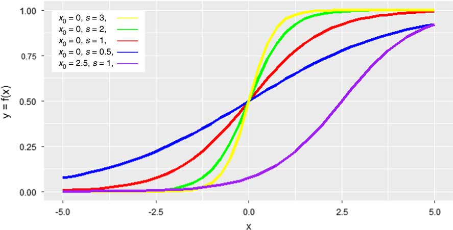
Fig. 1 Shapes of logistic functions, depending on the intercept position (x 0 ) and slope (s) values.
Transitions may show various gradualities in different directions across the interface, owing to the complexity of language contact, but fitting one global model (or trend) to the intensity values overlooks the regional variation. Therefore, a thorough comparison needs supporting analyses at local levels to characterize the true nature of the transition. Importantly, we apply models in spatial subsets, proposing dominance zones and transition zones, assuming the discovery of the homogeneous and inhomogeneous spatial subdivisions of variables, respectively.
5 Methodology
The proposed methodology relies largely on methods of curve and surface fitting, as used similarly in spatial analysis for trend surface and regression analysis, and is applied within three spatial scopes. First, the analysis extends over the entire study area (termed global level). Second, the analysis is conducted on spatial subsets, dependent on the distribution characteristics of the linguistic variable in question. Third, transitions are analyzed in profiles along cross sections. We used Esri ArcGIS 10.4 and the statistics scripting system R—packages akima (Akima & Gebhardt, Reference Akima and Gebhardt2016), ggplot2 (Wickham, Reference Wickham2016), landsat (Goslee, Reference Goslee2011) and rgl (Adler, Murdoch et al., Reference Adler2018) —for the analysis and illustrations of this work.
The following chain of methods demonstrates an increasingly fine-grained analysis. However, the methods involved can also be used independently as analytical tools for particular purposes.
Step 1: Variable selection. The conceptual model of viewing transitions between variants as gradients works best for dialectal variables that have two main variants that are ‘competing’ with each other in space. Importantly, these variables have to be distinguished from those where one main variant seems to occur almost everywhere in the study area, while other variants are reaching only regional dominance. Both of these variable types have been described by Glaser & Bart (Reference Glaser and Bart2015) for Swiss German syntax. The two main variants should also have their ‘core areas’ located preferably towards the edges of the study area, to assure the presence of one main interface between the two. Map 1 shows the intensity maps depicting eight of the syntax variables that have been selected for this work from the SADS and that represent the variable type of interest (see also Section 6.1). Table 1 gives a summary of these eight variables. While the intensity maps of Map 1 only depict the usage proportions (i.e., intensities) of the locally dominant variants, the proportions of all variants corresponding to a particular variable are used in the subsequent analysis, retaining the degree to which a certain variant becomes dominant or subordinate.
Table 1 The eight SADS variables shown in this paper. MC=multiple choice question, MV1=first main variant (red color in figures), MV2=second main variant (blue color in figures).
To find such variables, planar trend surfaces are fitted to the intensity surfaces of each variant, in order to establish the main aspect (i.e., compass direction) of the transition gradient. If the planar trend surfaces of two variants are inclined towards each other, that means that the two variants’ intensities complement each other, that is, the variants compete with each other at an interface. Calculating the aspect angles of these trend surfaces, variables with opposing aspects—that is, aspect differences close to 180° in their two main variants—are chosen as suitable for the proposed gradient fitting method. The aspect differences λ are calculated as λ=180°−|Aspect 1 -Aspect 2 | and are given in Map 1 for each variable.
Step 2: Intensity maps. Area-class maps (termed intensity maps here) can be used to chart the intensity values of variants, similarly to other studies (e.g., Rumpf et al., Reference Rumpf, Pickl, Elspaß, König and Schmidt2009). These maps use a Voronoi tessellation to spatially interpolate between the point locations of survey sites in order to obtain full spatial coverage, as often done in dialectometry (e.g., Goebl, Reference Goebl1982; J. Lee & Kretzschmar, Reference Lee and Kretzschmar1993; Rumpf et al., Reference Rumpf, Pickl, Elspaß, König and Schmidt2009). As noted above, Map 1 shows intensity maps for eight variables used in this work. The colors of the Voronoi polygons correspond to the locally dominant variant (except where no variant reaches dominance, in which case the color is grey). The brightness of the color corresponds to its intensity. Intensity maps have the drawback of only showing the locally dominant variants. Furthermore, it is hard to compare gradual transitions across maps based on colors. For example, the colors in the dominance zones can be lighter on average, still the transition itself may be relatively sharp (e.g., Question D in Map 1).
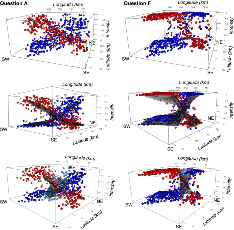
Step 3: Interactive 3-D plots. In order to reveal the intensity values of non-dominant variants, and to better understand the interplay of the different variants, interactive 3-D plots were generated (with rotation and zooming possible). Some examples are shown in a static version in Figure 2; an interactive version can be found in the online supplementary material. Beside the latitude and longitude values of survey sites, the intensities of the two main variants are used as the third dimension, similarly to a DEM.

Fig. 2 Static versions of the interactive 3-D visualizations representing intensity landscapes and different regression strategies. The top row presents the intensity values at each survey site, the middle row shows the fitted logistic models, and the bottom row shows the fitted planar regression surfaces in the transition zones. The cardinal directions on the plots (SW, SE, NE) indicate the survey sites’ geographic position. Interactive 3-D plots of these three types are shown in the online supplementary material for Questions A to H, with zooming and rotation possible.
Intensity maps (Map 1) and interactive 3-D plots (Figure 2) allow three initial observations. First, these visualizations demonstrate the existence of dominance zones and transition zones. For some variables the dominance zones seem to have more clear-cut boundaries, while for others the transition is more gradual (showing broad transition zones). Second, neither of these zones appear necessarily to be homogeneous. Third, the gradients of transitions are not uniform; patterns of change may be different at different positions and in different directions. This observation provides the motivation to also investigate the transition zones and the dominance zones separately.
Already based on these visualizations it seems possible to determine if sharp isoglosses characterize a certain variable. This allows making hypotheses about potential reasons for sharp boundaries and their locations. In addition, interactive 3-D plots allow us to see large- and small-scale trends in the intensity surfaces, and thus to make more informed qualitative statements about the spatial patterns present.
Step 4: Model fitting. Using intensity values as the third dimension, a logistic model can be spatially fitted to the intensity landscape. Function stats::glm in R uses iteratively reweighted least squares (IWLS) for the fitting. The returned model parameters and derived measures quantitatively describe the model, which is a smoothed representation of the variants’ intensity surfaces, characterizing the main trends of the main transitions. The comparison across variables is possible based on the slope value of these logistic models. The deviance measure represents the fit in a logistic regression model analogously to the sum of squares calculations in linear regression analysis (Hosmer, Taber & Lemeshow, Reference Hosmer, Taber and Lemeshow1991). The smaller the deviance, the better the fit. Because the model is always fitted to data from all survey sites, it is possible to compare across variables based on these models. The surface model can also be visualized in the interactive 3-D plots using its fitted values (Figure 2), allowing visual comparison.
Step 5: Profile analysis. In order to get an impression of local characteristics beside global gradient properties, and to analyze the transitions in different directions, the intensity landscapes are also investigated in profiles along cross sections (similarly to Burridge, Reference Burridge2017:14; Davis & Huock, Reference Davis and Huock1992; Girard & Larmouth, Reference Girard and Larmouth1993).
Profiles are constructed across the study area along straight lines, which are placed in the aspect angle of the main direction of change. More precisely, the direction of the profile is equivalent to the bisecting angle of the two main variants’ aspect angles, as they oppose each other in small, acute angle differences (λ) indicated in Map 1. Several parallel profiles are constructed to better cover the study area and to potentially represent the different transition characteristics and gradualities in different parts of the study area. In this work, for each variable, four profiles were placed at stratified random distances (Map 2; cross sections are numbered from NW to SE). The final step of the spatial construction of profiles is shown in Figure 3. The profile line is intersected with the Voronoi polygons of survey sites. Then, for each line segment bounded by a polygon, the midpoint is computed, and the intensity value of the polygon is assigned to the midpoint, resulting in an intensity profile.
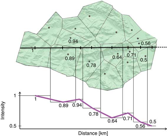
Fig. 3 Constructing profiles in geographic space and registering the intensity values of a fictive variable along the cross section (2-D map view and profile view).
Logistic curves are then fitted to the intensity profiles of the main variants. While the deviance value gives the goodness of fit of the model, the slope and intercept values characterize the graduality of the transition and its position. To characterize the profile more by its variation in intensity in the particular direction, a volatility measure is calculated by the summed change in intensity along the profile. In the fictive example of Figure 3, the intensity changes (0.11+0.05+0.16+0.14+0.07+0.15+0.06) would add up to a volatility value of 0.74. The volatility value accumulating along a profile is usually at least 1, as intensity values normally range from 1.0 to 0.0 along the profile, and more survey sites are involved than in the simple example of Figure 3. The relative volatility is given by dividing the volatility value by the number of survey sites along the profile. In the case of Figure 3 this would come to 0.74/8=0.0925. Since in the relative volatility, values have been normalized, they can be compared across profiles.
Step 6: Gradient subdivisions. In the type of variables examined, the gradient change is expected to occur predominantly in transition zones, as opposed to dominance zones. Two subdivision strategies are proposed to investigate the validity of the two conceptual models of dialectal transitions (isoglosses vs. dialect continua), and thereby test the isogloss hypothesis, for each individual variable.
The first subdivision strategy consists of a bipartite subdivision, in which two partitions are established at the level of the entire study area. In this strategy, a dense grid is first interpolated for each of the two dialectal variants using kernel density estimation (KDE) smoothing (Sibler et al., Reference Sibler, Weibel, Glaser and Bart2012). Then, for each pixel, the dominant of the two variants is determined. The line separating one dominant variant from the other then forms the isogloss that can be used to subdivide the study area into two partitions. The survey sites falling into either of these partitions are then passed separately to the trend model fitting operation, fitting a different planar model (linear model in case of the profiles) to each of the two partitions.
Bipartite subdivisions serve to test the dialect continuum concept or isogloss concept, respectively, by calculating the sum of squared residuals (SSR) to the constants 1.0 and 0.0. These are the expected intensity values in the respective dominance zones of the two main variants, in a perfectly binary spatial distribution (i.e., in the isogloss scenario).
Conversely, the tripartite subdivision strategy defines two dominance zones and a transition zone in between, based on the intensity profiles. As the linguistic literature does not formally define outer boundaries of transition zones, we attempt a definition based on unequivocal dominance. The boundaries of a transition zone for each profile are defined by a steep drop in the intensity in the two variants, with the following rules: 1) In order to define a transition zone, both variants’ intensity values need to approach the expected values (0.0 and 1.0) along the profile (i.e., there has to be a marked change in intensity values); 2) the boundary is placed at the largest intensity value change (drop) along the profile; 3) if there are several similar intensity changes, the one after which there is no more substantial increase present is used. Additionally, if less than two survey sites would be assigned to a transition zone (i.e., if the support is too small to allow fitting a trend model), only the two dominance zones are created.
To construct the tripartite subdivisions at the level of the entire study area, the breakpoints calculated in the four corresponding profiles of a particular dialectal variable are connected by their spatial coordinates, taking into account further local patterns of the transition present between the breakpoints in the intensity maps. Then, each survey site in the study area is assigned to one of the three partitions it falls into. Fitting of trend models to dominance zones is carried out in the same way as performed for the bipartite subdivision strategy.
In addition, a planar trend surface (or planar trend line in profiles) is fitted in the transition zone, to model the change assumed to be happening in this area. Several measures are then calculated for the fitted trend in the transition zone. The slope of the fitted function characterizes the gradual nature of the transition. The goodness of fit of the planar model is given by the SSR. Besides, the width of the transition zone is given as the geographic distance along the profile between the threshold points in the two main variants. The volatility and the relative volatility are also calculated. For the fitted planar trend surfaces, additionally the average of the widths in the four corresponding profiles is obtained.
6 Results
6.1 Patterns of Transition in Intensity Maps
Based on the values of aspect differences (shown also in Map 1), about 40% of the variables in SADS are eligible to be analyzed with our methodology. In this section, results for a subset of eight variables (Table 1) are shown, representing typical patterns of transitions, including diverse gradualities and different overall directions of transition. From each respondent, only the variant with which they most strongly associated was taken into account.
Four out of the eight survey questions—Questions A, B, C and D, addressing the phenomenon infinitival purposive clause—were already used in other studies involving the authors (Jeszenszky, Stoeckle, Glaser & Weibel, Reference Jeszenszky, Stoeckle, Glaser and Weibel2017; Sibler et al., Reference Sibler, Weibel, Glaser and Bart2012). Questions A, B, C were also used by Seiler (Reference Seiler2005). The answers to the questions regarding the infinitival purposive clause reveal two main competing variants ‘für’ and ‘zum’ (shown in red and blue, respectively, in the top four maps of Map 1) and also some minor variants, including the Standard German variant ‘um… zu’ (shown in green). All four infinitival purposive clause questions feature the dominance of the ‘für’ variant (red) in the southwest, while the ‘zum’ variant (blue) is dominant in the northeast of the study area. Importantly, transitions between the two main variants occur in different regions of the study area, with different gradualities observable. In Question B, notably, the red ‘für’ appears to dominate the southwest less than in other variables. Further, the ‘um…zu’ variant (green), plays a more important role in Question A than in Questions B to D. This and other subordinate variants seem to be more randomly distributed in space than the main variants.
The remaining four survey questions (Questions E to H in Table 1) are related to different syntactic phenomena. Question E and Question F, respectively, deal with the position of the non-finite verb in perfect tense and in the infinitive particle (Jeszenszky & Weibel, Reference Jeszenszky and Weibel2015; Scherrer, Reference Scherrer2012). Question G addresses the occurrence of the infinitive particle (Stoeckle, Reference Stoeckle2018) and Question H relates to the adnominal possessive.
The expected transition patterns based on exploratory analysis using intensity maps and interactive 3-D visualization (similar to those shown in Map 1 and Figure 2, respectively, along with the supplementary material) are included in Table 1. The variables represented by Questions A, B, C and, to a certain degree, D seem to show a gradual transition, while Questions F and G are typical representatives of variables with a sharp transition. Questions E and H also show gradual transition patterns but at certain locations sharp transitions are further visible. Also, in Question G both main variants have small areas embedded in the dominance zones of the opposing main variant, where they become locally dominant.
The general direction of transitions, as visible in Map 1 and reflected in the placement of profiles in Map 2, is southwest – northeast (SW–NE), also corresponding to the direction of the main population corridor of the densely populated Swiss Plateau. In contrast, Question H represents another main trend of transition, occurring in the N–S direction and reflecting the cross section from the Alps to the Swiss Plateau, which is also characteristic in Swiss German (Haas, 2000:61-63).
6.2 Logistic Regression Surfaces
Logistic models were fitted to the intensity surfaces of each main variant (e.g., Figure 2, middle row, and supplementary material). The slope values calculated for each surface are given in Table 2. In a typical isogloss scenario, high slope values are expected, and the more gradual the transition, the lower slope values are expected. The fit of the model to the intensity surfaces is given by the deviance value. Lower deviance values mean a better fit. Also, comparison across logistic models is more reliable when their deviance values are lower.
Table 2 Slope and deviance (goodness of fit) values of the global logistic models.
6.3 Patterns in Intensity Profiles
In the eight variables presented, each profile incorporates 17 to 37 survey sites into the linear subset of their intensity profiles (median=26), with Question H having the shortest profiles and hence encompassing the least survey sites.
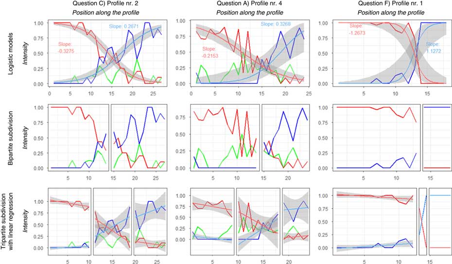
Figure 4 presents a typical gradual transition (Question C) in the left column, a sharp transition (Question F) in the right column, and a somewhat undecided transition pattern (Question A) in the middle column. It is interesting to note that above we described Question A as one with a gradual transition at the global scale (Table 1), but this particular profile (A4, cutting through parts of the Alps) in Figure 4 exhibits a rather noisy pattern. The intensity values of the two main variants are given taking all other variants into account (such as the values of the ‘um… zu’ variant, which are also plotted, in green). In the top row, the fitted logistic regression curves are displayed along with their slope values. In the middle and bottom rows, respectively, subdivisions resulting from the bipartite and tripartite subdivision strategies are presented, with the linear model fitted in the latter. Bipartite subdivisions show two fairly homogeneous areas for Question F, while for Questions A and C the split between the two dominance areas does not mean exclusive usage of the locally dominant variants. In the tripartite subdivision it is visible that by defining a transition zone the dominance zones can be kept more homogeneous and the undecided patterns are more confined (i.e., they remain in the transition zone).
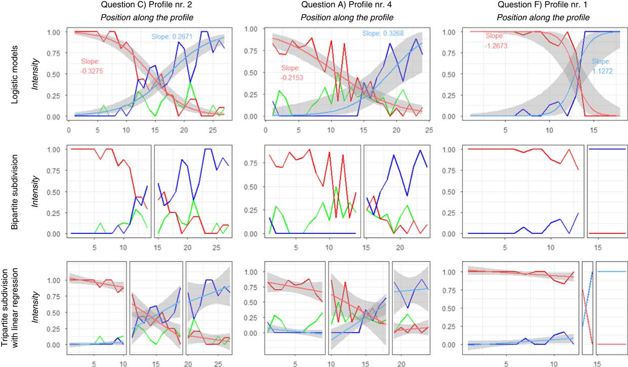
Fig. 4 Profile analysis: profiles corresponding to typical transition patterns in theories: left column – gradual transition (dialect continuum), right column – sharp transition (isogloss). The middle column shows a profile with more mixed patterns. Red and blue lines, respectively, are used to depict the two main variants, while green is used for a third, minor variant (if present). The top row also presents the fitted logistic regression curve for the two main variants, with the 95% confidence band shown in grey. The middle and the bottom row show the subdivisions resulting from the bipartite and tripartite strategies with linear trendlines fitted in the latter.
The slope values of the logistic curves in the intensity profiles are given in Table 3, along with their deviance values, the position of the intercept (relative to the midpoint of the profile), the volatility and the relative volatility for Questions A, C and F.
Table 3 Parameters (slope and intercept) and goodness of fit (deviance) values of the logistic regression curves in intensity profiles (numbered as shown in Map 2), along with the volatility measures of the intensities. The rows highlighted by black frames correspond to the profiles shown in Figure 4. Negative steepness means sloping towards right. Deviance and volatility are color coded based on their values. Green values correspond to better fit and to less change in intensity along the profile. Barplots indicate if slope values of the logistic models are sloping towards the left (red variant of Figure 4) or right (blue variant). The barplots illustrating intercept values correspond to the position of the logistic models’ inflection point relative to the geographical midpoint (0) of the profile (with -1 and 1 indicating the left and right endpoints of the profile, respectively). MV2 in F4 is an extreme outlier, having a perfect sharp transition in this profile, therefore in the slope column has its cell fully colored in blue. In A1, the logistic function in MV2’s model is so elongated towards the right that its intercept position is outside the profile.
6.4 Patterns in Subdivisions
In the dominance zones resulting from both spatial subdivision strategies, fits of the planes corresponding to maximal intensity and zero intensity values are calculated. The fits are given as SSR for both main variants, in their respective dominance zones as deviation from a plane of 1.0 (meaning 100% intensity) and in the opposing dominance zone from a plane of 0.0 (0% intensity). Table 4 presents these SSR values, for Questions A, C and F, similarly to Figure 4. An ideal sharp transition in a variable would show values close to zero in the second and third columns in both main variants (MV1 and MV2). And in the case of a perfect isogloss scenario, the values for the bipartite and tripartite subdivision would be equal, as no transition zone could be defined in the tripartite case.
Table 4 Goodness of fit values (sums of squared residuals – SSR) in the spatial subsets. The smaller the value, the better the planar surface fits the expected value given in Section 5, Step 6. Dom-1=the dominance zone of MV1, Dom-2=the dominance zone of MV2. Questions A, C and F are the example variables used in Figure 4.
Table 5 presents the findings of the tripartite subdivision at the scale of the entire study area, showing the slope and fit values (SSR) of planar trend surfaces fitted in the transition zones, along with the average of the transition zone widths in the four intensity profiles.
Table 5 Spatial subsets: slope and goodness of fit values (SSR) of planar regression surfaces in the transition zones resulting from the tripartite subdivision, together with the average width of transition zones in intensity profiles. For Question B only three transition zones were found, while for Question F, only two. Barplots indicate the slope of the trend surface (the longer the bar, the steeper) and the average width of the transition zones (the longer, the wider). Fit values are color coded, with green indicating the best fit.
Significance of the slope values deviating from 0.0: *** p<0.001, ** p<0.01, * p<0.05
Table 6 presents the results of the subdivision analysis in the intensity profiles by giving the slope and fits (SSR) of the linear models fitted in the transition zones, along with the widths of the transition zones (in km), the volatility and the relative volatility in the transition zones.
Table 6 Subsets in intensity profiles: slope and goodness of fit values (SSR) of linear regression in the transition zones resulting from the tripartite subdivision, together with the volatility, relative volatility, and width of the transition zones. Questions A, C and F are the example variables used in Figure 4. Barplots illustrate slope values of the logistic models sloping towards the right and left, representing the red and the blue variants in Figure 4, respectively. Barplots are also used to show the width of the transition zones: the longer the bars, the wider the transition zone. SSR and volatility values are color coded. Green values correspond to better fit and to less change in intensity along the profile, respectively.
In the intensity profiles of typical isogloss scenarios (Figure 4, lower row, right) the tripartite subdivisions may become very similar to the bipartite subdivision, causing narrow transition zones (such as in the case of Question F).
7 Discussion
The main aim of this work is the quantitative characterization of transitions at the interface of dialectal variants, which allows comparison across variables. The methods proposed address this issue from the point of view of gradients. We model the spatial variation of dialectal variants with the spatial application of S-shaped curves often described in the temporal dimension in the fields of dialect contact and language change (Blythe & Croft, Reference Blythe and Croft2012; Willis, Reference Willis2017; Yokoyama & Sanada, Reference Yokoyama and Sanada2009).
As the focus of this paper is on developing methods that could be generalized to be applied on different databases, the discussion concentrates on evaluating the performance of the proposed methods and their implications for dialectological research, rather than the linguistic interpretation of the results. In the following, we will discuss the main quantitative results in the light of the theoretical expectations and the supplementary measures. First, however, we will briefly turn to the role of visualizations in supporting qualitative analysis.
7.1 Visualizing Dialectal Transitions
While not a methodological contribution per se, the intensity maps (Map 1) and particularly the 3-D plots (Figure 2 and supplementary material) used in this article have shown the potential to facilitate an initial understanding of the spatial variation present in different dialectal variants, and the transitions between them. Visualizations also facilitate developing hypotheses regarding the nature of transitions. For the SADS variables used in this work, in most cases it is easy to see in the visualizations that the hypothesis of the presence of sharp isoglosses can be discarded. Nevertheless, using these simple maps and plots, trained analysts may already be able to identify the cases where isoglosses are genuinely present. However, solely based on visualizations no quantitative comparison is possible.
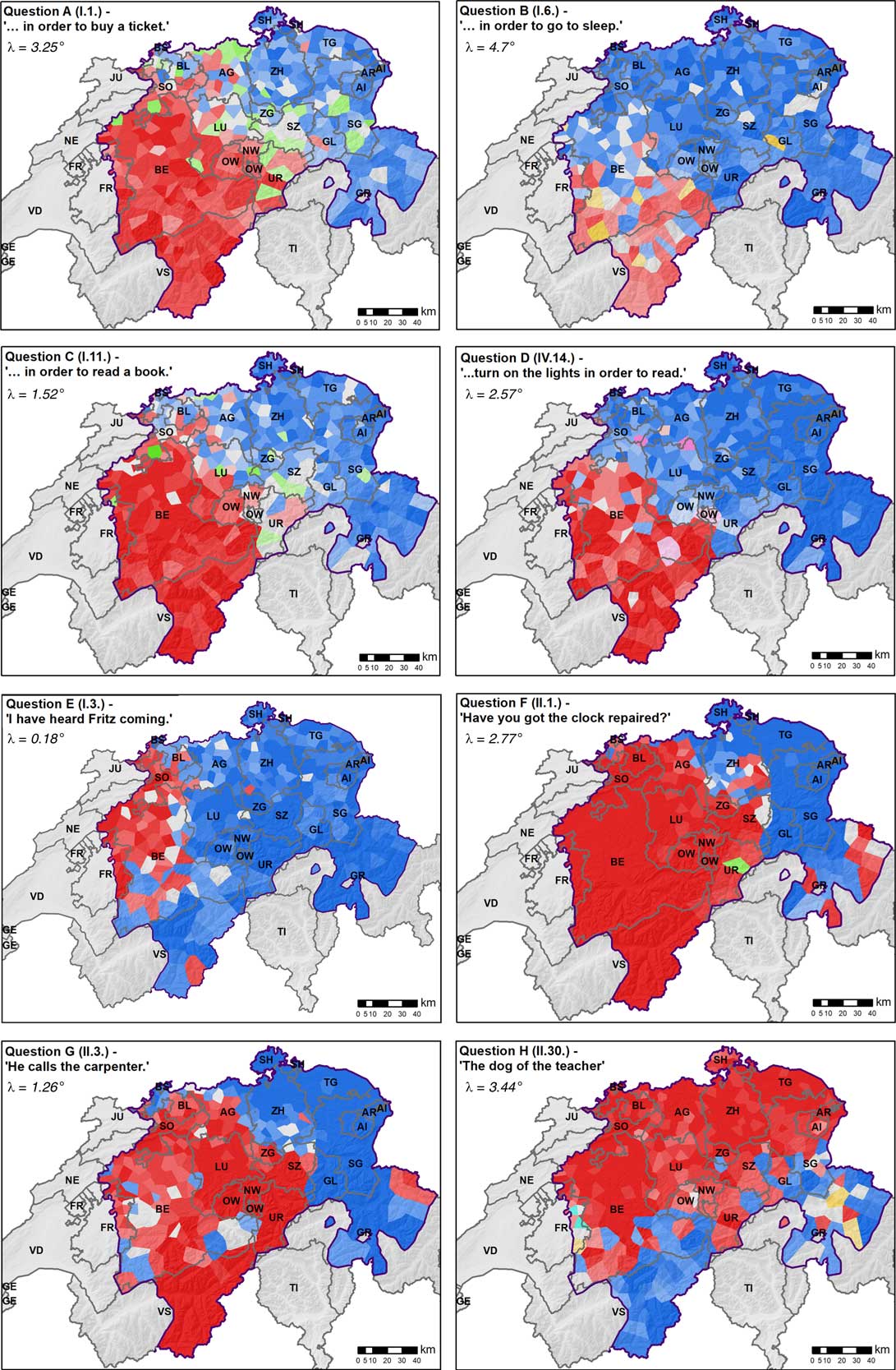
Map 1 Intensity maps of eight variables used, along with the aspect differences (λ) calculated in Step 1.
7.2 Modeling Spatial Transitions Using Logistic Models
The S-curve model, often used to characterize transition in the temporal dimension, was assumed also to have a spatial manifestation in the shape of a wave (e.g., C.-J. Bailey, Reference Bailey1973; Britain, Reference Britain2002; Willis, Reference Willis2017). As a cross section of a wave resembles the shape of a logistic function, the use of logistic regression model fitting is intuitive. Willis (Reference Willis2017) uses three types of logistic regression models, a global (non-geographic) logistic regression, a logistic regression model based on geographic administrative units, and logistic models fitted using geographically weighted regression (GWR), in an apparent-time study of the spatial diffusion of morphosyntactic change. While Willis’ study focused on the temporal dimension of the diffusion process, we propose to use logistic regression as a spatial model, focusing on the shape of the logistic model as fitted to the underlying intensity values, and as characterized by a set of descriptive measures. Our focus is thus on the transition zones.
Since at the level of the whole study area the logistic models are always fitted to the same set of points and the density of points is generally consistent throughout the study area, the models can be compared using their slope parameter (Table 2). The goodness of fit of the logistic surfaces is given by the deviance value, which depends on the homogeneity in the variant’s intensity values, thus on the degree of spatial variation in the given variant. Questions E to H have large deviance values, meaning poorer fit of the logistic regression surface. Regarding slope values, typical representatives of gradual and sharp transitions (Question A: 0.4339 and 0.4793, and Question F: 1.0531 and 1.1603 respectively) correspond to the expectations raised by the visualizations (last column in Table 1). This is, however, not always true about the other variables: in cases of high deviance, slope values can be less reliably determined, as there is more spatial variation and hence more uncertainty involved. For example, Question G, which, by inspecting the intensity map (Map 1), was characterized as having a sharp transition (Table 1), shows some of the lowest slope values (0.4211 and 0.4156) in Table 2. This is due to additional areas of mixture beside a main transition, towards the western part of the study area (e.g., canton Berne - BE).
Using a ‘single number’ to characterize dialectal transitions falls short of rendering the complex nature of such mixture zones. Thus, we now turn to the results obtained from applying the proposed supplementary measures, analyzing the transitions at different, more local scopes.
7.3 Profile Analysis
Patterns identified in the four intensity profiles constructed for each variable can contribute to the interpretation of the intensity maps and the measures obtained from the analysis at the global level. In Table 3, three rows are highlighted by a frame, showing a typical gradual (C2), a typical sharp (F1), and a more variable transition (A4), corresponding to the profiles shown in Figure 4.
In Table 3, slope and deviance values in general correspond to the expectations (Table 1) based on the visualizations, with Question F having high slope values (all above 0.4, as also shown by the longer horizontal bars and outliers), while the gradual transition variables of Questions A and C, reach relatively low slope values (between 0.11 and 0.34, respectively). At the same time, the highlighted A4, C2 and F1 profiles show relatively low deviance values, indicating a good fit (and cells filled in greenish colors). F1 has one of the steepest logistic curves recorded, coupled with a good fit, confirming its typical sharp transition. For other profiles, slope values seem to show a mixed picture, which might indicate the sensitivity of regression to the rather low number of intensity values (17 to 37) making up the profiles, and transition trends having diverging characteristics in different profiles. Low deviance and volatility values would indicate if intensity values perfectly fitted the logistic model, regardless of their slope. Conversely, higher values (e.g., the relative volatility values mean 10.46% to 17.18% average change for each step in Question A, and 9.85% and 14% for C3) indicate the presence of fluctuations, therefore fuzzier transition patterns.
The intercept (which may range between -1 and 1) gives an indication of the position of the inflection point of the logistic function relative to the geographical midpoint in the profile. In other words, this value informs us about the symmetry of the two MVs and helps compare the spatial patterns of variables belonging to the same phenomenon. For this reason, we use horizontal bars in Table 3 to show both the magnitude and relative position of the intercepts. The majority of intercepts is located to the right of the geographical midpoint, indicated by blue color (the color of MV2; cf. Map 1). This is true for all of the MV2 intercepts, and only 4 out of 12 intercepts of MV2 are located to the left. This either hints, as in the case of Questions A and C, at the weaker dominance of these variants, or shows that their dominance is confined to a smaller area (Question F).
Intensity values tend to fluctuate along the profiles, forming local peaks and depressions, often deviating from the fitted logistic and linear regression curve (Figure 4). This variability is measured by the volatility (and relative volatility) values in intensity profiles. For the three variables presented in Table 3, the sharp transition F1 profile shows low relative volatility values (green hues), whereas the A4 profile, characterized as an undecided pattern, shows a higher value (red hues) for MV1 and a lower value for MV2, illustrating the different types of transition patterns playing together in these profiles. Note that the absolute volatility values also depend on the survey sites visited along the profiles. Thus, a certain bias may be present and relative volatility is preferred for comparisons between different variants and variables.
7.4 Bipartite and T ripartite Subdivisions
One contribution of the bipartite and tripartite subdivision strategies is to show how much of the spatial transition is confined to a particular transition zone. Table 4 shows the fits of expected values according to the two subdivision strategies. The expectation in the bipartite strategy is for intensity values of both main variants to be maximal (1.0) in their respective dominance zones and minimal (0.0) in the opposing dominance zone. The same is expected in the tripartite strategy with the difference that a transition zone comes in between, assumed to hold most values other than 0.0 and 1.0, in an ideal case. For Question F, consistent SSR values are seen in the bipartite strategy (all around 11.75), which means that the residuals are evenly distributed in the two dominance zones. For Questions A and C, SSR values are in all cases higher in their respective dominance zone than in the opposing dominance zone, which means that there is better correspondence to the expectations with regards to the absence of a variant than to its dominance. In the tripartite strategy, the SSR values are lower in general, meaning that a lot of survey sites with intensities other than 0.0 or 1.0 are located within the transition zone. This effect is much stronger, however, for Questions A and C, where the SSR values drop dramatically in the tripartite strategy compared to the bipartite strategy. This suggests that the tripartite subdivision strategy is useful in characterizing the transitions between dialectal variants.
Widths. In this work, transition zone widths are the most important supplementary measures. In Table 6 narrower transition zones (as also indicated by horizontal barplots) imply that the transition is happening in a spatially more restricted area, suggesting a sharper transition. Small average transition zone widths and lacking transition zones (i.e., not determinable for all four profiles) in Table 5 suggest an isogloss scenario, while wider transition zones are assumed to correspond to more gradual transitions.Typical variables with gradual transition (Questions A, C) have widths above 50 km on average, while sharp transition variables (Questions F, G) stay typically below 30 km on average and have missing transition zones (Tables 5 and 6, respectively).
Although up to four transition zones per variable contribute to the average width, the results of the width measure should be interpreted with some caution, as the actual values depend on the placement of the profiles and the determination of drop points may be affected by the variability of intensity values concerned. Nevertheless, the width measures do contribute to the greater picture of characterizing the graduality of transitions in different directions.
Trends. Linear trends in transition zones of profiles were determined in order to help confirm the fuzzy nature of transition zones and to gauge if most of the transition is indeed confined to the transition zones. Table 6 gives the numerical values of slopes found in the transition zones of the tripartite subdivisions, and it further visualizes the magnitude and direction of the slopes by colored bars. In this table, for example, both slopes for A1 are negative, meaning that the transition zone’s trend is so different from the global trend that not even their slope directions (aspects) correspond. In narrow transition zones, these linear models also typically do not show a significant fit, contrary to wider transition zones, which are more often marked by asterisks to indicate significance of slope values. In Table 5, characterizing the transition zones resulting from the spatial subdivision, the planar model fits (SSR) to transition zones show rather poor values, regardless of the widths of the transition zones, hinting at the presence of rather high variability of intensity values in the transitions. These planes, however, have significant slopes (Table 5), except for Question E and H (which were both described as ‘mixed pattern’ variables in Table 1). In the significant cases, which correspond to the variables described in Table 1 as having either sharp or gradual transitions, the slope values help quantify the strength of the transition. For example, Question G’s sharp looking main transition is not found in Table 2 due to the mixture present, but through the tripartite subdivision it becomes visible in the slope values of Table 5 and is further supported by transition zone width values.
Volatility. Volatility indicates the presence of variation and thus shows why some fits are poorer than others. In Tables 3 and 6, volatility often vastly exceeds the value of 1, the value corresponding to an ideal (i.e., monotonic) transition, indicating that fluctuations are present in the corresponding transitions. If the volatility in the transition zones in Table 6 was equal to the volatility in the entire intensity profile (Table 3), it would indicate that the entire transition is happening within the transition zone. For example, for the two MV of F2, 1.87 and 1.97 in the transition zone (Table 6) out of the 1.97 and 2.08 in the entire profile (Table 3), respectively, means that roughly 95% of volatility values in the entire intensity profile are confined to the (narrow) transition zone. At the same time this proportion is relatively low for profiles A2 and A3 (i.e., between 48% and 74%), indicating that fluctuations occur both in the transition zone as well as the dominance zone. Transition zone widths also help the interpretation of volatility, as volatility values in Table 6 have, of course, more chance to reach higher values in a wider transition zone. In case intensity values do not reach the two extremes (0 or 1), volatility can, theoretically, also stay below 1. Relative volatility is, however, instantly comparable across variables, showing the average intensity change with each step in the profile. Comparing relative volatility values between Table 3 and Table 6 reveals that the values for Question F in Table 6 are about four to five times higher than those in Table 3, which, knowing the widths of transition zones, indicates a very sharp change in the transition zone. For Question A, the increase in relative volatility values between Tables 3 and 6 is usually less than double, indicating a more gradual transition.
7.5 Implications for Linguistic Research
It is the contact between people that drives the natural change in language, including the propagation of a new variant within and beyond linguistic communities (e.g., Chambers & Trudgill, Reference Chambers and Trudgill2004; S. Lee & Hasegawa, Reference Lee and Hasegawa2014). Thus, there is a very strong spatial component to language change. Based on contact patterns between people, one could hypothesize about the spatial and linguistic characteristics of change and type of transition to be expected. Hence, given the influence of topography, the transportation system and the prevailing mobility patterns of the Swiss population, for the SADS data, one could hypothesize wider transition zones and more gradual transitions in the flatter Swiss Plateau (German: ‘Mittelland’) with a more mobile society and minimal topographic barriers, contrasted by sharper transitions in mountainous areas. We believe that the methods presented here could be of help in testing this, and similar, spatially inspired hypotheses, in particular the methods proposed for directional (intensity profiles) and regional analysis (spatial subdivisions), coupled with exploratory visualizations.
The proposed methods enable more informed decisions, but of course cannot replace the expertise of the trained dialectologist. With the quantification of the spatial transitions, supported by different visualizations as shown in this article, one may identify the variables worth investigating more in detail and the scenarios that are more interesting to study from the point of view of language change and dialect contact. Knowing the gradients in different variables may help testing diffusion-related hypotheses (Willis, Reference Willis2017). For example, sharp boundaries would indicate a more static relationship between two variants while a gradual transition would hint at ongoing change. For instance, inspired by Glaser’s (Reference Glaser2013:214) observation concerning Swiss German morphosyntax mentioned in Section 4, testing if trends move towards a usage of mixed grammar with both variants could be interesting. The possibility of comparing linguistic variables with regards to their transitions facilitates inferences concerning areal patterns with respect to their relationships. Thus, the methods proposed allow the identification of patterns of similar and different areal behavior of linguistic variables, assisting the development of further questions regarding the dialect contact mechanism for different linguistic phenomena (and possibly different time frames). Further, the quantitative methods help linguistic analysts test hypotheses based on the visualization of large volumes of data points.
Demonstrating the practical usability of the proposed methodology, the infinitival purposive clause (Questions A-D), can be characterized and compared based on the results reported in Section 6. In the intensity maps (Map 1), each of them appears to show a gradual transition, with Question D possibly having a somewhat sharper transition. Although the four questions address the same linguistic phenomenon, the transitions happen at different locations. Questions A and C are similar with regards to their transitive linguistic structure, and their intensity maps show similar spatial patterns as well (Map 1). Questions B and D also have similarities with regards to grammatical structure, as neither of the purposive clauses include an object. Still, their differences in transition patterns do not fully reflect this similarity, contrary to intuitive expectations (cf. Labov et al., Reference Labov, Ash and Boberg2006:305). Comparing the slope values of the spatial logistic models of each main variant (Table 2), the MV1 of Question D has the sharpest transition, followed by MV1 in Question B, both also showing the smallest deviance values. These observations allow the development of hypotheses on potentially ongoing language change or a tendency of merging grammars, with the patterns of this transitional behavior being different depending on factors like grammatical context and the function the variable plays in the language (as discussed in Glaser, Reference Glaser2013; Seiler, Reference Seiler2004:380, 2005). Logistic models in the profiles of Questions A and C (Table 3) present significant differences with regards to slope values across profiles (A4 MV2 – 0.3268 vs. A1 MV2 – 0.1119; C4 MV2 – 0.3402 vs. C3 MV2 – 0.1734, with both A4 and C4 profiles located in the Alps, as shown on Map 2). Besides, their volatility values show significant differences along the profiles (Table 3). This might stem from different isolation and contact factors acting in different areas and might indicate the uncertainty and bias engrained in the profiles’ construction. Table 5 shows highly significant slope values for Questions A to D, with very varied slope values in the transition zones, however. This observation is also somewhat visible in the intensity maps but confirmed by the interactive 3-D visualizations in the supplementary material.
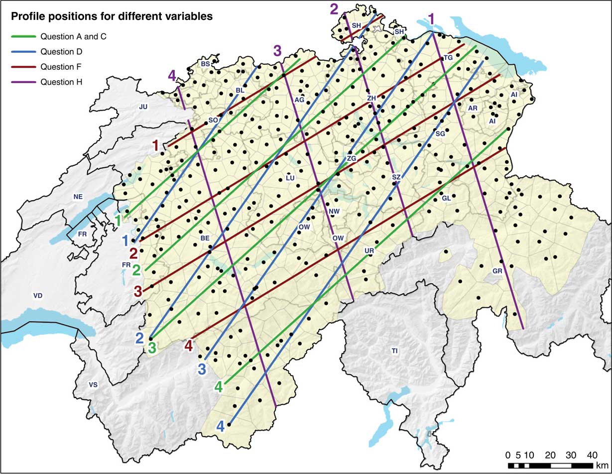
Map 2 Intensity profile positions, overlaid on the SADS survey site map.
7.6 Limitations
One clear limitation of the methodology is that it can only be used to characterize the transition between exactly two variants belonging to a variable, at a single interface. This type of configuration, however, is not uncommon, particularly in morphosyntax (Glaser, Reference Glaser2013; Willis, Reference Willis2017). Hence, the proposed approach has the potential to be applied rather widely.
The drawback of fitting logistic surface functions to intensity surfaces is that they are the spatial extension of the logistic curve, fitting a single, unidirectional ‘wave’ (as visible in Figure 2), meaning that only one transition can be explained in a variable. Therefore, the study area for the application of the logistic model should ideally be chosen not to include other areas of mixture, in order to focus on the actual transition in question. More subtle, gradual transitions occurring in certain areas, such as those described by Seiler (Reference Seiler2005), however, can still be quantified with this method without having to arbitrarily delineate the transition zone.
Spatial subsetting, as performed in profile construction as well as in the spatial subdivision strategies, mean a reduced number of survey sites included in subsets, leading to increased local uncertainty and causing some model fits to be non-significant. On the positive side, the paucity of survey sites in narrow or non-existent transition zones established in tripartite subdivision may also serve as an indicator of sharp transitions.
Some bias in intensity profiles stems from the construction of the profiles (Figure 3). Geographic distances between reference points of polygons (the midpoints of the transecting line in each polygon) do not correspond to the actual Euclidean distance between neighboring survey sites. Also, the order in which survey sites are linked after one another along the profile might not follow natural paths of contact, especially in mountainous areas. The tripartite subdivision strategy, however, handles this bias to a certain degree by taking the fluctuation of intensities into account when defining transition zones.
8 Conclusions
This work introduced a methodology consisting of a set of methods and measures which aim to support the quantitative characterization of spatial transitions in dialectal variables. Conceptualizing transitions between areas of dialectal variants as gradients, and using logistic model fitting as our main tool, we have been able to make the following methodological contributions:
As the proposed methodology is suited primarily for dialect variables with two main competing variants (Figure 2), we have developed a method that allows the automatic detection of such variables in a database, fitting a planar trend surface to each variant and determining the difference in their main aspect angles.
We have devised a method for logistic surface fitting to the intensity values of dialectal variants. We have further proposed a method for profile construction from intensity values, and logistic curve fitting to these profiles.
While the slope of the fitted logistic function is arguably the most important descriptive parameter, as it is the basis of comparison across variables and it directly relates to the question of whether or not a particular dialectal transition resembles an isogloss, we have proposed a number of supplementary measures that allow the characterization of different aspects of transitions, including: the intercept of the logistic function; the deviance (goodness of fit) of the logistic model to the actual intensity values; the volatility and relative volatility; and the width of the transition zone.
We have developed two different spatial subdivision strategies that allow testing for the presence of isoglosses, with the bipartite subdivision assuming a perfect isogloss model, with no transition zone present, and the tripartite subdivision assuming a transition zone.
The proposed approach of fitting logistic models represents a spatial counterpart to using logistic functions in the temporal dimension in the field of language contact and change (e.g., Kroch, Reference Kroch1989; Willis, Reference Willis2017; Yokoyama & Sanada, Reference Yokoyama and Sanada2009). Through these methods, it becomes possible to quantitatively compare different dialectal variables regarding their prevailing transitions. With the support of several supplementary measures, a more informative and differentiated quantitative characterization of the dialectal transitions is possible, bearing in mind that the complexity of dialectal transitions cannot be fully rendered by a single characteristic. In particular the tripartite subdivision strategy helps demarcate transition zones, where most of the change is supposed to take place between dominance zones of dialectal variants, and thus may allow the development of hypotheses about diffusion and grammar merging in dialects. Thus, the methods proposed allow the grouping of variants based on their behavior in the transition zones.
Since assumptions are only made with regard to the spatial distribution of the input data, the methodology is potentially generalizable to further linguistic levels or other spatial variables with appropriate spatial granularity.
Several directions for future research may be noted. As a direct extension, residual maps could be generated for visual diagnostics. Mapping the residuals of the logistic models in the intensity landscape, and thereby the goodness of fit, could help assess the patterns of the transition and the spatial distribution of the variants (Beale, Lennon, Yearsley, Brewer & Elston, Reference Beale, Lennon, Yearsley, Brewer and Elston2010). As another extension, transitions can be tested for respondents in different age groups, unravelling ongoing dialect change based on the apparent time construct (e.g., G. Bailey et al., Reference Bailey, Wilke, Tillery and Sand1991; Willis, Reference Willis2017). Also, the robustness of spatial patterns could be tested by Monte Carlo simulations. Beyond direct improvements, the proposed methods and measures could be applied to other dialect databases to evaluate whether they are also applicable to other study areas and data configurations. Similarly, the methodology could also be applied to the study of transitions between opposing categorical variables in other fields, such as demographics or soil science. And finally, it would also be interesting to compare the boundaries of dominance and transition zones to extralinguistic geographical boundaries.
Supplementary material
To view supplementary material for this article, please visit https://doi.org/10.1017/jlg.2019.1
Acknowledgements
The research reported in this paper partly represents the PhD project of the first author. Funding by the Swiss National Science Foundation through projects “Modeling morphosyntactic area formation in Swiss German (SynMod and SynMod+)” (SNF Project no. 140716 and no. 162760) is gratefully acknowledged. We are grateful to Gabi Bart and Sandro Bachmann of the Syntactic Atlas of German-speaking Switzerland (SADS) project for the provision and professional help with the linguistic data. Further, we would like to thank the comments of the anonymous reviewers and the editors of the Journal of Linguistic Geography.