

1. Introduction
In dialectology, the neogrammarian tradition of describing a single local dialect with all the relevant features through an Ortsgrammatik (i.e., a grammar of a local dialect) was still prevalent in the first half of the twentieth century (Murray, Reference Murray, Auer and Erich Schmidt2010). Around the same time, however, the tradition of dialect geography evolved, where the spatial distribution of linguistic features or lexemes were mapped and interpreted (Schrambke, Reference Schrambke, Auer and Erich Schmidt2010). Originally, dialect geography focused on mapping single linguistic features or single lexemes one at a time (Girnth, Reference Girnth, Lameli, Kehrein and Rabanus2010). In the late twentieth century, this approach was criticized and accused of missing general patterns of dialect variation (Wieling et al., Reference Wieling and Nerbonne2015). At the same time, language atlases became available, and novel computational methods were developed, which sparked the development of dialectometry, a quantitative branch of dialect geography (Nerbonne & Kretzschmar, Jr., Reference Nerbonne and Kretzschmar2013). Dialectometry explores the general spatial variation of dialects using distance or similarity measures rather than single features (Goebl et al., Reference Goebl, Jaberg and Gilliéron1984).
Dialectometry was first introduced by Séguy (Reference Séguy1973) who analyzed the dialectal variation in the Gascogne in southwest France using the Hamming distance metric (HD) (Hamming, Reference Hamming1950), which captures the co-occurrence of linguistic features at different locations. Later, Goebl (Reference Goebl1982) introduced the Weighted Identity Value (WIV), a similarity measure that also accounts for the rareness of a linguistic feature. Both HD and WIV take categorical or nominal features as inputs, which makes them especially well-suited for syntactic and morphological data. For example, HD was used to explore the syntactic variation in Dutch (Spruit et al., Reference Spruit2008) and French dialects (Goebl, Reference Goebl, Lameli, Kehrein and Rabanus2010). By contrast, Levenshtein distance (LD) takes strings or words as input. LD computes the minimum number of single-character operations (insertions, deletions, or substitutions) required to change one string to another (Levenshtein, Reference Levenshtein1966). LD was first introduced to dialectometry by Kessler (Reference Kessler1995) and was later used to measure phonetic and lexical distances between dialect variants, such as in Dutch (Heeringa, Reference Heeringa2004), Norwegian (Gooskens et al., Reference Gooskens and Heeringa2004), and Catalan (Valls et al., Reference Valls, Nerbonne, Prokić, Wieling, Clue and Rosa Lloret2012).
HD, WIV, LD, and other distance and similarity measures gave rise to the use of cluster analysis to explore dialect variation. Cluster analysis partitions a set of objects into similar groups, such that distances within the group are minimized while distances between groups are maximized. Initially, researchers predominately applied hard-clustering methods to dialect data, such as Hierarchical Clustering (Goebl, Reference Goebl2008; Prokić et al., Reference Prokić and Nerbonne2008; Scherrer et al., Reference Syrjänen, Honkola, Lehtinen, Leino and Vesakoski2016; Szmrecsanyi, Reference Szmrecsanyi2011) or k-means clustering (Lundberg, Reference Lundberg2005). Hard- clustering assigns each object to a single group, generating clear-cut boundaries between groups. Thus, hard-clustering methods miss out on gradual variations in continuous dialect data.
In contrast, dimensionality reduction (DR) aims to reduce the number of variables in a dataset while preserving the variation as much as possible. DR allows for mapping complex patterns in high-dimensional data to low-dimensional space. Methods of dimensionality reduction, such as Multidimensional Scaling, Principal Component Analysis, and Factor Analysis have been applied to explore patterns in dialect data (Embleton, Reference Embleton1993; W. J. Heeringa, Reference Heeringa2004; Nerbonne, W. Heeringa, et al., Reference Nerbonne, Heeringa and Kleiweg1999; Pröll et al., Reference Pröll, Pickl and Spettl2014; Shackleton Jr., Reference Shackleton2005). While DR appropriately reflects dialect continua, the resulting patterns are not always informative, since the remaining dimensions might not fully capture the variation in the data (Wieling et al., Reference Wieling and Nerbonne2015). More problematic still, there is no direct way of mapping visual patterns to explicit clusters.
Unlike DR, Bayesian clustering (BC) both captures the gradual variation in dialects and returns explicit clusters instead of mere visualizations. In BC, the assignment of objects to clusters is fuzzy: each object belongs to every cluster with a certain probability. Bayesian clustering yields core regions where objects predominantly belong to a single cluster and gradual boundaries where objects belong to multiple clusters with almost equal probabilities. BC was initially developed in evolutionary biology: the STRUCTURE algorithm aims to infer population structure from individual genotypes and gene frequencies (Pritchard et al., Reference Pritchard, Stephens and Donnelly2000). Genotypes are usually admixed. Due to genetic exchange, individuals carry genetic information from several different populations. Using Markov Chain Monte Carlo sampling (MCMC), STRUCTURE estimates both the unknown populations and the degree to which an individual belongs to each population.
Spatial Bayesian clustering (Durand, Jay, et al., Reference Durand, Jay, Gaggiotti and François2009; Chen et al., Reference Chen, Durand, Forbes and François2007; Corander et al., Reference Corander, Sirén and Arjas2008, Guillot et al., Reference Guillot, Mortier and Estoup2005) is largely based on the Structure algorithm, but, in addition, accounts for spatial trends—the systematic increase or decrease of a variable along a spatial axis, and spatial autocorrelation—the similarity of neighboring objects in space. While BC has been applied to both languages and dialects, including Tasmanian (Bowern, Reference Bowern2012), Sahul (Reesink et al., Reference Reesink, Singer and Dunn2009), Melanesian (Dunn et al., Reference Dunn, Levinson, Lindström, Reesink and Terrill2008), and Finnish (Syrjänen et al., Reference Syrjänen, Honkola, Lehtinen, Leino and Vesakoski2016), spatial Bayesian clustering has not yet been applied to linguistic data. This is surprising, especially given that geography has long been identified as a key factor of dialect variation (Nerbonne and Kleiweg, Reference Nerbonne and Kleiweg2007).
In this article, we contribute to closing this research gap. We apply TESS (Chen et al., Reference Chen, Durand, Forbes and François2007; Durand, Jay, et al., Reference Durand, Jay, Gaggiotti and François2009), a spatial Bayesian clustering algorithm, to Swiss German dialect data. The data are adopted from the Syntaktischer Atlas der deutschen Schweiz (SADS) (Bachmann et al., Reference Bachmann, Bart and Glaser2021; Glaser & Bart, Reference Glaser and Bart2021). The SADS data comprise syntactical and morphosyntactical constructions in Swiss German, seeking to complement the Sprachatlas der deutschen Schweiz (SDS) (Hotzenköcherle, Trüb, et al., Reference Hotzenköcherle and Trüb1962–2003), which largely focuses on lexical items as well as phonological and morphological features. Recently, several studies have used quantitative methods to explore both the SDS and SADS data (see Bart et al., Reference Bart, Glaser, Sibler and Weibel2013; Jeszenszky, Stoeckle, et al., Reference Jeszenszky, Stoeckle, Glaser and Weibel2017; Kellerhals, Reference Kellerhals2014; Leemann, Reference Leemann2016; Scherrer et al., Reference Syrjänen, Honkola, Lehtinen, Leino and Vesakoski2016; Sibler et al., Reference Sibler, Weibel, Glaser and Bart2012).
TESS models admixture levels using both global trends and local spatial autocorrelation. We test three different models: (1) a nonspatial model, largely equivalent to the original Structure algorithm; (2) a spatial trend model, which accounts for global spatial trends in the admixture levels; and (3) a spatial full-trend model, which accounts for both global trends and local spatial autocorrelation. We apply all three models to the SADS data, evaluate their performance, and identify the most suitable model for inferring clusters.
2. Dialectal and biological populations
Parallels in biological and linguistic evolution were already noted by Darwin (Reference Darwin1859), and many analogies between the two fields have since been made, especially between biology and dialectology. While unrelated or distantly related varieties (“languages”) are investigated at a macrogeographic scale, the study of closely related varieties (“dialects”) looks into microgeographic areas where speakers can understand each other without significant effort. Related dialect speakers are what is called mutually intelligible and, thus, likely to influence each other and interchange linguistic features (Hock et al., Reference Hock and Joseph2009; Reesink et al., Reference Reesink, Singer and Dunn2009), leading to analogous processes as observed in evolutionary biology, as summarized in Figure 1.
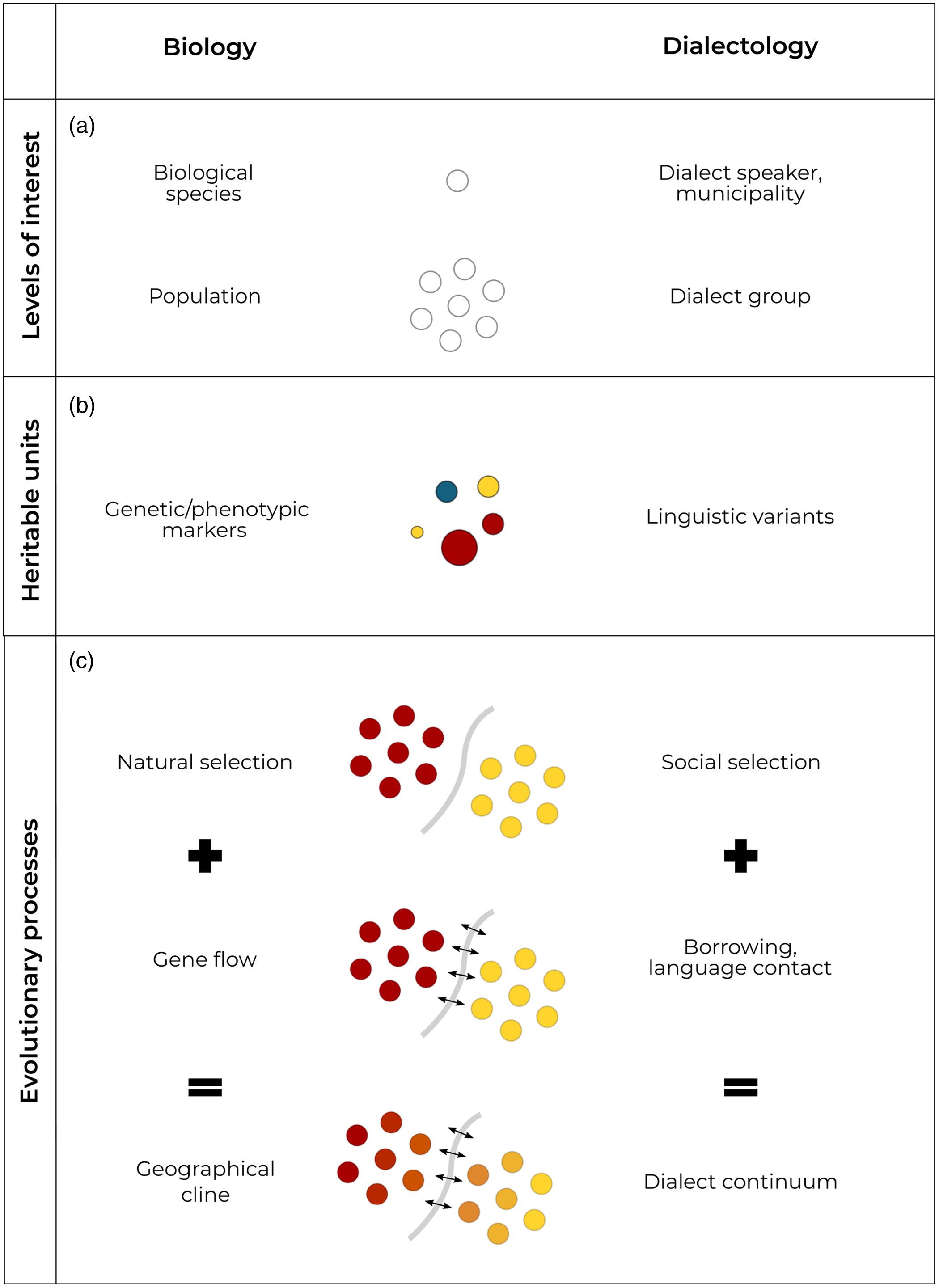
Figure 1. Parallels between biology and dialectology. Table adapted from Atkinson (Reference Atkinson and Gray2005).
Biological populations and dialect groups undergo similar evolutionary processes (Figure 1.C). Natural selection occurs when species adapt to a specific environment and their genetic information changes across generations. A similar process can be found in dialects in the form of social selection (Atkinson et al., Reference Atkinson and Gray2005; Pagel, Reference Pagel2009), for instance caused by the presence of administrative boundaries or natural barriers. Gene flow occurs when two distinct biological populations come into contact and transfer genetic information between populations (Jobling et al., Reference Jobling, Hurles and Tyler-Smith2013). The counterpart of gene flow in linguistics is termed borrowing (Atkinson et al., Reference Atkinson and Gray2005; Pagel, Reference Pagel2009), which can occur when languages or dialect speakers from different regions come in contact and influence each other. As was explained above, borrowing is more likely between related languages and dialects. In biology, gene flow opposes the divergent force of selection in the areas where populations come into contact, thus blurring interpopulation transitions. This leads to the formation of geographical clines, a gradual change in a biological trait across space. Similarly, a dialect continuum results from the mutual intelligibility between neighboring dialects; the linguistic difference between dialects increases with distance and vice versa, creating a continuum rather than discrete boundaries.
These parallels show that treating dialect data analogous to genetic evidence is far from arbitrary. From a data perspective, dialectal phenomena are expected to be continuous and dialect groups are likely admixed due to borrowing and contact. Bayesian clustering is tailored to finding populations in admixed traits, making it well-suited to cluster dialect data.
3. Materials and methods
3.1 Data
The Syntaktischer Atlas der deutschen Schweiz (SADS) (Bucheli et al., Reference Bucheli and Glaser2002; Glaser & Bart, Reference Glaser and Bart2015) was created to capture the morphosyntactic variation in Swiss German. Between 2000 and 2002, a total of three thousand participants in 383 Swiss German-speaking municipalities were surveyed, with three to twenty-six individuals per municipality (median value of 6.5). The SADS data are particular in that they have multiple samples per municipality, while comparable data campaigns only interviewed a single respondent per spatial unit (Jeszenszky & Weibel, Reference Jeszenszky and Weibel2015), leading to less robust conclusions about linguistic variation. For this study, only respondents with a known geographic origin were considered, resulting in 2,970 individuals (Map 1) for which 211 morphosyntactic variants were collected. From these we derived the variables for the analysis, of which ultimately eighty-eight moderately associated variables were used for clustering (Figure 2).
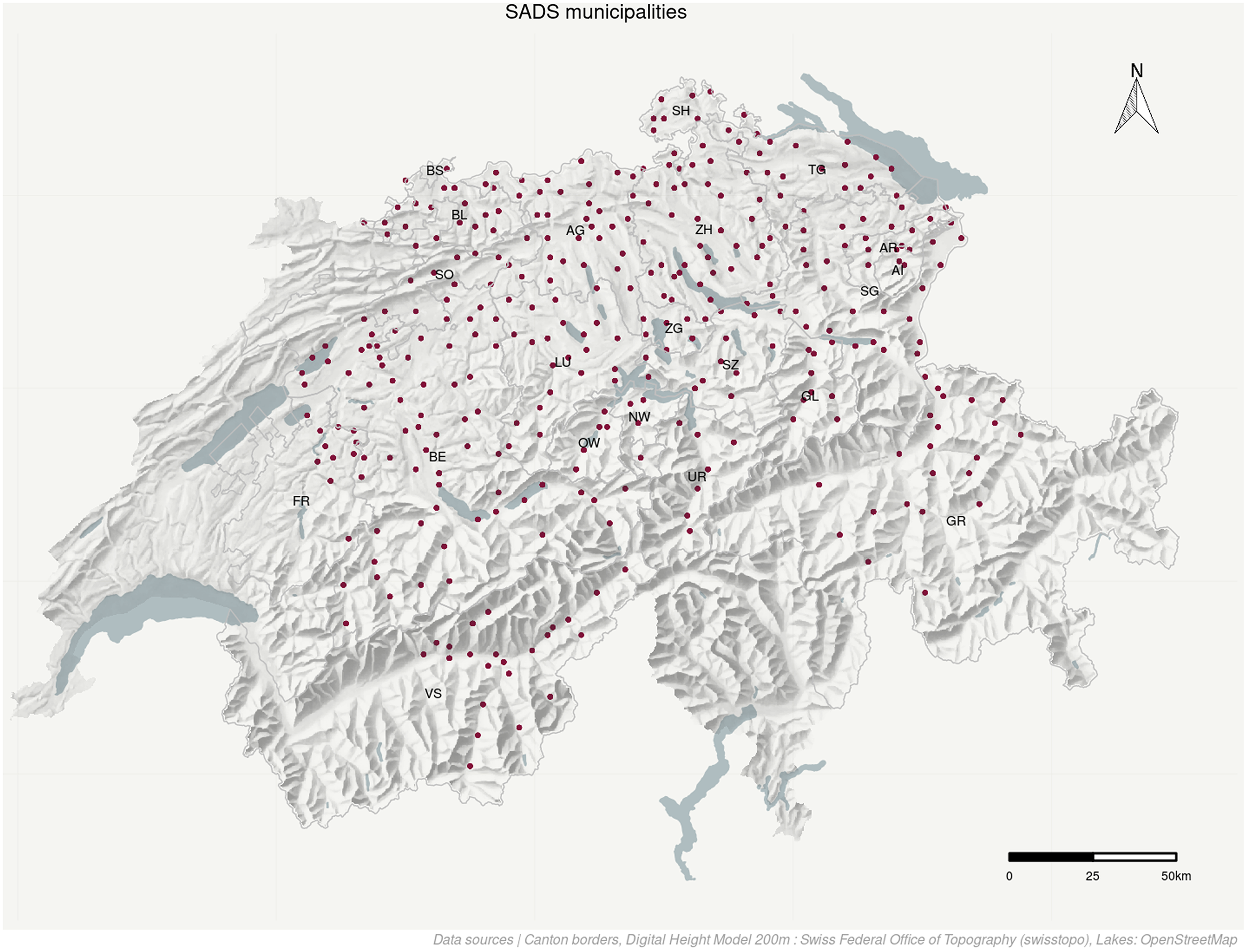
Map 1. All municipalities in the SADS data
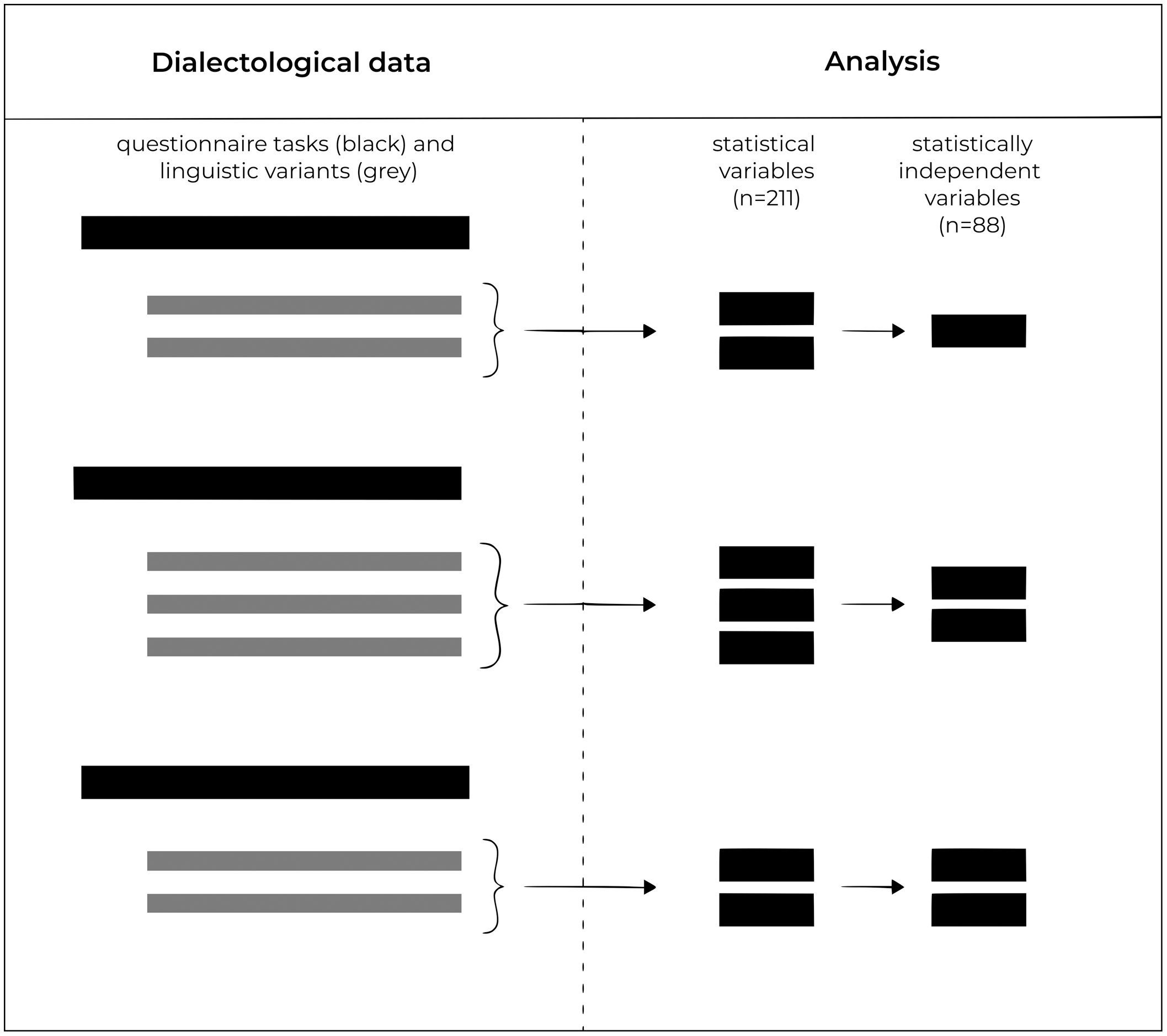
Figure 2. Pre-processing the dialectological data: the SADS derives linguistic variants from questionnaire tasks. These serve as statistical variables for the analysis, of which only the statistically independent ones were used for Bayesian clustering.
3.2 Population structure
We applied TESS 2.3 (Chen et al., Reference Chen, Durand, Forbes and François2007; Durand, Jay, et al., Reference Durand, Jay, Gaggiotti and François2009) to cluster the dialect data. TESS is a spatial Bayesian clustering algorithm inspired by STRUCTURE, a widely used algorithm in population genetics to infer population structure from multilocus genotype data. TESS assumes that individuals have mixed ancestry, such that each individual has traits from at most K max populations. A so-called admixture model infers the unknown ancestral populations, which—having been in continuous contact with each other–—give rise to individuals with mixed ancestry. For Swiss German extensive interdialectal contact is expected, which is why we consider the admixture model well-suited for clustering the SADS data.
When inferring ancestral populations, TESS assumes alleles at different loci to be independent within populations, which is referred to as linkage equilibrium in evolutionary biology. This biological assumption cannot be fully paralleled in linguistics since linguistic features are not carried in a specific physical location such as loci in biology. However, the strong association between linguistic variants could be interpreted as a linkage disequilibrium state. We computed Cramer’s V to measure the association between all morphosyntactic features in the SADS data and retained only those that were moderately associated (V ≤ 0.3). While moderate correlations in the data improve the clustering, strong correlations could lead to biased, overly confident clusters and overestimate the number of inferred populations (Falush et al., Reference Falush, Stephens and Pritchard2003; Kaeuffer et al., Reference Kaeuffer, Réale, Coltman and Pontier2007). For comparison, we also performed the cluster analysis on the full dataset, resulting in similar but overly clear-cut clusters (see supplementary materials).
TESS 2.3 incorporates spatial priors to account for global and local spatial effects. Global spatial priors assume that the influence of population K changes gradually along a spatial trend surface with gradients β K . Local spatial priors assume that the probability of an individual to belong to population K depends on its spatial neighbors. We tested three models with different spatial priors (Durand, Jay, et al., Reference Durand, Jay, Gaggiotti and François2009):
-
the nonspatial model without a spatial prior (similar to STRUCTURE);
-
the spatial trend model with global spatial priors;
-
the spatial full-trend model, with both global and local spatial priors.
TESS estimates population structure using Markov Chain Monte Carlo (MCMC) sampling. For the SADS data, 30,000 iterations were sufficient for the MCMC to converge to a stationary distribution. We discarded the first ten thousand iterations as burn-in, ensuring to sample from high probability regions. We tested different numbers of ancestral populations (K ∈ 2, …, 8). For each K we ran fifteen independent runs. To have better estimates for the individual admixture proportions (Durand, Chen, et al., Reference Durand, Chen and François2009), the results were averaged over the five best runs using the software CLUMPP (Jakobsson et al., Reference Jakobsson and Rosenberg2007).
3.3 Model performance
TESS provides a statistical measure—the Deviance Information Criterion (DIC)—for testing which model and which number of ancestral populations best fit the data (Durand, Jay, et al., Reference Durand, Jay, Gaggiotti and François2009; Spiegelhalter et al., Reference Spiegelhalter, Best, Carlin and Van Der Linde2002). The DIC comprises two terms: an estimate of model fit and an estimate of the effective number of parameters, which for TESS correspond to the number of ancestral populations K. There is a trade-off between model fit and the number of parameters: increasing K improves the fit, making it easier to capture the variation in the data but at the same time makes the model more likely to overfit and pick up random noise in the data. In general, the lower the DIC, the better the model. As a rule of thumb, the most suitable number of populations is where the DIC levels off, such that adding more populations decreases or only marginally improves performance.
4. Results
4.1 Number of ancestral populations
Figure 3 shows the DIC for K ∈ 2, …, eight for the nonspatial model, the spatial trend model and the spatial full-trend model averaged over the five best runs. For all three models, the DIC levels off between five and seven populations. For K > 5 the spatial trend model outperforms the nonspatial model. For K > 6 the spatial full-trend model outperforms all other models.

Figure 3. Average Deviance Information Criteria (DIC) of the five best MCMC runs for each model. The DIC levels off between five and seven populations. For K = 5 the spatial trend model outperforms both the spatial full-trend model and the nonspatial model.
The purpose of cluster analysis is that of generalization: we apply TESS to reveal the main patterns of dialectal diversity in Swiss German morphosyntax.
If supported by the data, large clusters are preferred over small ones as they provide a higher level of generalization and, thus, deeper linguistic insights not apparent from the raw data. Considering that there is at best a moderate increase between K = 5 and K = 7 over all three models, we concluded that five populations best explain the structure in the data. For K = 5 the spatial trend model outperforms all other models. In the next section, we present both the spatial distribution of all five population clusters and their spatial trends. For comparison, we provide additional results for K = 6 in the supplementary materials.
4.2 Spatial distribution of populations
Population 1 (Map 2) is predominantly present in canton VS and becomes gradually less present toward the border with BE in the north, the eastern part of FR, and some municipalities in the center of Switzerland (for Swiss canton codes see Table 1). The population continues eastward through OW, NW, SZ, and UR, eventually reaching the canton of GR. We refer to this population as Oberwallis population.

Map 2. Admixture proportions of Oberwallis population
Table 1. Swiss canton codes

Population 2 (Map 3) covers most municipalities in the cantons of BE and FR. The population spreads upward to BS and BL in the north, the border to VS in the south, and to ZH and SZ in the east. As the core of the population is in BE, we refer to this population as the Bern population.

Map 3. Admixture proportions of Bern population
Population 3 (Map 4) has its core in northern Switzerland (canton SH) and gradually decreases in frequency to the cantons SO, LU, UR, OW, GL, SG, AI, and AR in the south. Accordingly, we label it as Northern population.
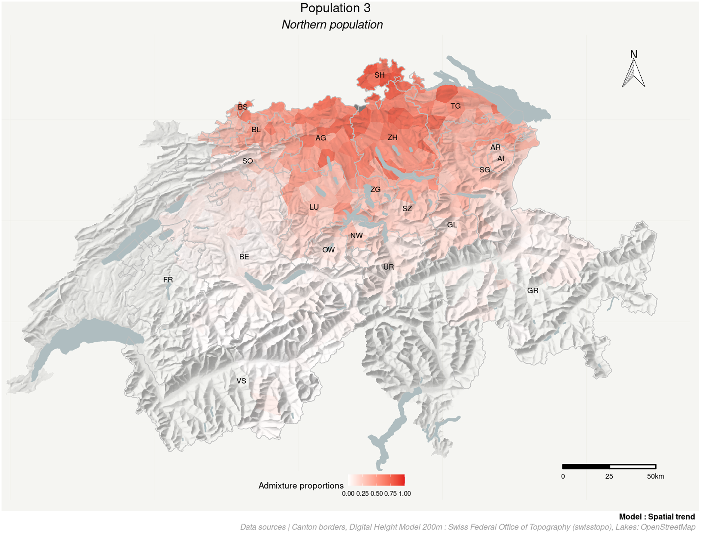
Map 4. Admixture proportions of Northern population
Population 4 (Map 5) does not show a distinctive spatial pattern. It lacks a clear core, and most municipalities seem to partly belong to it. Therefore, we refer to this population as the Swiss base population.
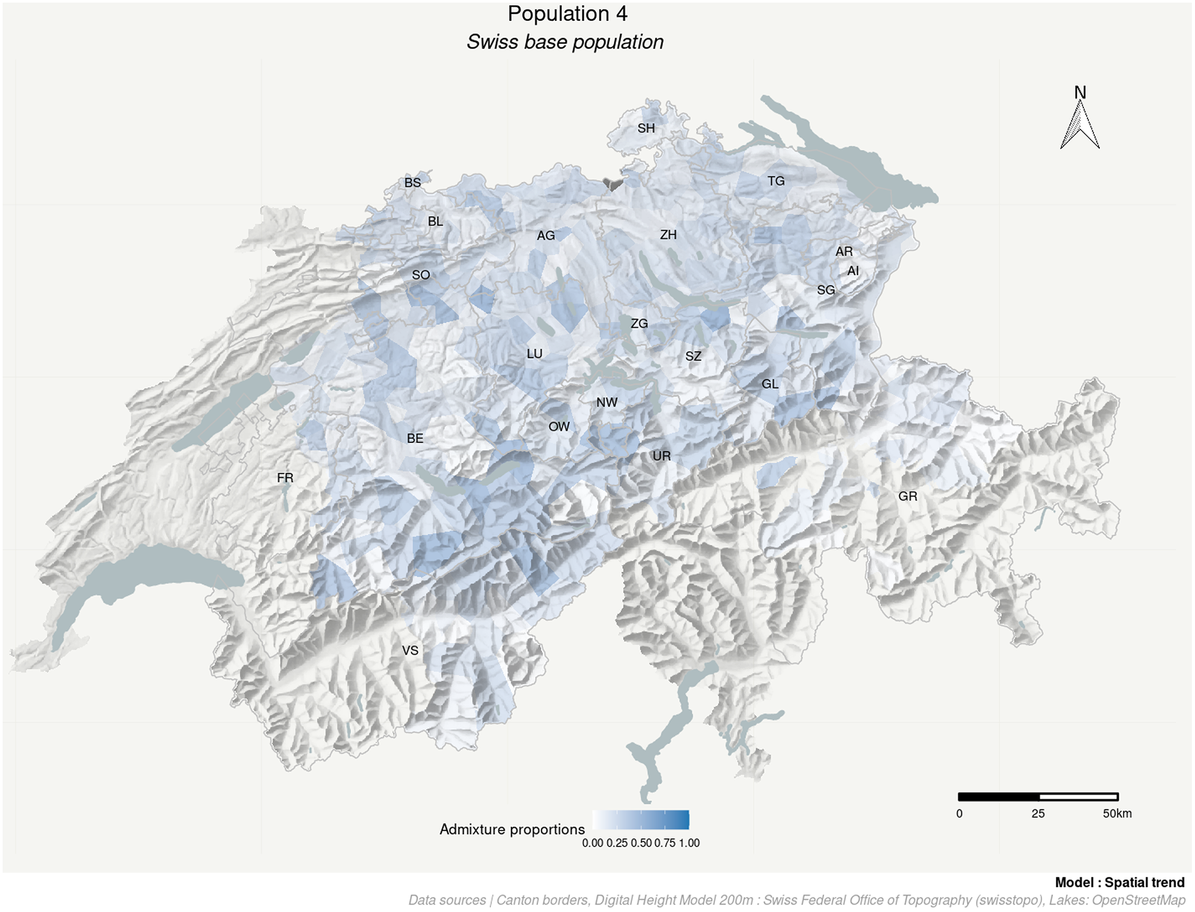
Map 5. Admixture proportions of Swiss base population
Population 5 (Map 6) is located in the southeastern part of Switzerland. Its core is in GR from where it continues to cantons UR, LU, AG, ZH, SH, and TG, gradually decreasing toward the west. Therefore, we label the population as the Graubünden population.

Map 6. Admixture proportions of Graubünden population
4.3 Spatial trends
The β coefficients quantify the magnitude of the trend surface in the spatial trend model. Table 2 shows the β coefficients and their relative Credible Intervals (CI) for all five populations.
Table 2. β estimates and relative Credible Intervals (CI). Positive β long represents west to east trends, meaning that the admixture proportions increase eastward. Positive β lat represents south to north trends, meaning that the admixture proportions increase northward

The Oberwallis population has a significant southward-pointing latitudinal trend but no longitudinal trend (the CI of β long includes 0). On the contrary, the Bern population shows a significant westward-pointing longitudinal trend but no latitudinal trend. The Northern population has a significant northward-pointing latitudinal trend with no longitudinal trend. The Swiss base population does not show any spatial trend (the CI of both β long and β lat trend center around zero). The Graubünden population has small but significant latitudinal and longitudinal trends.
5. Discussion
We identified five populations in the SADS data, for which the spatial trend model outperforms both the nonspatial and the spatial full-trend model. When comparing admixture levels of the municipalities to traditional dialect regions (Hotzenköcherle, Bigler, et al., Reference Hotzenköcherle, Bigler, Schläpfer and Börlin1984), we find four correspondences: the areas of dialectal populations 1, 2, 3, and 5 match the four traditional dialectal macroregions constituted by bundles of North-South and East-West isoglosses (Glaser, Reference Glaser2014:25–26; Christen et al., Reference Christen, Glaser and Friedli2019:29–30). Population 4, on the contrary, can be interpreted as a “base” population, which has left traces in all Swiss German dialects. Population 1 (Oberwallis population) corresponds to the dialect region commonly classified as Highest Alemannic, whereas populations 2, 3, and 5 together are commonly classified as High Alemannic (Hotzenköcherle, Bigler, et al., Reference Hotzenköcherle, Bigler, Schläpfer and Börlin1984).Footnote 1
In traditional dialectology and folk linguistics, dialect boundaries are usually discrete rather than gradual (Stoeckle, Reference Stoeckle, Sandra Hansen, Stoeckle and Streck2012), as they are constructed by few salient, overlapping isoglosses. This is also the case for Swiss German dialects. In contrast, the populations in our study do not exhibit clear-cut boundaries since grammar—and to a certain extent even single linguistic features (Seiler, Reference Seiler2005:330–33)—show gradual transitions (Glaser & Bart, Reference Glaser and Bart2015:90–92). Similar findings have also been made by other quantitative studies on Swiss German. Jeszensky and Weibel (Reference Jeszenszky and Weibel2016) show that syntactic features often show gradual transitions, even for individual features.
Depending on the linguistic feature and the way the data were collected, individual variables can show both crisp or gradual boundaries (Glaser, Reference Glaser2014; Jeszenszky, Stoeckle, et al., Reference Jeszenszky, Stoeckle, Glaser and Weibel2018; Scherrer et al., Reference Scherrer and Stoeckle2016). Bayesian clustering is flexible enough to adapt to the signal in the data and faithfully identifies both gradual transitions and clear-cut boundaries. On the contrary, discrete clustering will always yield discrete dialect regions, which in some cases “may not be an accurate representation of reality” (Grieve et al., Reference Grieve, Speelman and Geeraerts2011).
Concerning the spatial distribution of the populations, our results correspond to those by Kellerhals (Reference Kellerhals2014), who identified similar dialect regions in the SADS data (depending on the method sometimes represented by more than a single area). Scherrer et al. (Reference Scherrer and Stoeckle2016) compare the SADS data to phonological, morphological, and lexical data from the SDS and prove that all three follow a similar spatial distribution. The traditional dialect boundaries have also been confirmed recently by Lameli et al. (Reference Lameli, Glaser and Stoeckle2020) using data from the Deutsche Sprachatlas (Wenker et al., Reference Wenker, Lameli, Heil and Wellendorf2013).
Four out of the five populations show an evident spatial structure with clear cores and a gradual increase of admixture toward the center. The β coefficients (Table 2)—which correspond to the spatial gradient of the admixture levels—are always oriented in the direction of the core: southward for the Oberwallis population, westward for the Bern population, northward for Northern population, and eastward for the Graubünden population. This is in line with the wave model of Schmidt (Reference Schmidt1872), which claims that language traits spread gradually from a central point.
The cores of the clusters are located at the borders of the study area and admixture gradually increases toward the center. This suggests that there is more dialect diversity—with respect to the features in the SADS—in the center of the study area and less so at the borders. We compute the Shannon diversity index (H), a statistical measure of diversity (Shannon, Reference Shannon2001), to further test this. Map 7 shows that the least diverse municipalities with the lowest H are indeed located at the edges of the study area and overlap with the cores of the four populations, whereas the most diverse municipalities with the highest H are in the center.

Map 7. Dialectal diversity expressed in terms of the Shannon diversity index (H)
In this study, we treat dialect features as heritable units (Syrjänen et al., Reference Syrjänen, Honkola, Lehtinen, Leino and Vesakoski2016), analogous to genotypic and phenotypic markers (Figure 1). Our findings show that this analogy is indeed reasonable. The spatial pattern of the Oberwallis population (Map 2), for example, reflects one of the most relevant historical migration events in Swiss history known as the Walser migration. Due to particular sovereign rights in the area (Waibel, Reference Waibel2013), several groups of people emigrated in the 13–15th centuries from the Oberwallis to the Berner Oberland, Uri, and Graubünden (Lessmann-Della Pietra, Reference Lessmann-Della Pietra, Bachmann and Glaser2019; Waibel, Reference Waibel2013). The migration of the Walser population to Northern regions corresponds to a spread of dialects with Highest Alemannic features. The lighter areas in Graubünden in Map 6 would then be explained by the layering of the Oberwallis population with its Highest Alemannic features as a superstratum on top of the more prevalent Graubünden population. At the same time, the lighter areas in Fribourg and Central Switzerland in Map 3 would be explained by a case of substratum layering, where the Oberwallis population’s dialects are superimposed by Bern population dialects. This pattern is confirmed in Map 2: the core of the cluster is in VS, from where it continues toward the east along the migration corridor, reaching municipalities in the cantons UR and GR.
Bayesian clustering rests on several assumptions that must be met to yield meaningful results. We briefly summarize how our analysis satisfies these assumptions. First, the analysis is based on a sufficient number of linguistically independent features, which are likely to cause balanced and unbiased populations. The dialect sample is dense and evenly distributed over the study area, which is key for estimating both spatial trends and spatial autocorrelation. All dialects are related and are likely to belong to a single continuum. This in line with the objectives of the admixture model and the DIC, which aim to assign data points to as few meaningful clusters as possible. Reliable information about the historical background of the dialects is available and was used as an implicit prior to decide for an optimal number of clusters (Brooks et al., Reference Brooks, Smith, Vehtari, Plummer, Stone, Robert, Titterington, Nelder, Atkinson and Dawid2002). Finally, TESS infers populations that are as close as possible to Hardy-Weinberg equilibrium (HWE). HWE assumes that the allele frequencies in populations do not change between generations, which in the context of dialects implies that ancestral linguistic features do not change over time. This assumption seems contradictory for dialects in contact, which are likely to interchange features and are expected to evolve faster than biological populations (Boyd et al., Reference Boyd and Richerson2005; Dawkins, Reference Dawkins1976). If HWE does not hold, the resulting clusters might not adequately represent ancestral populations but rather reflect current population structure. This is why one must be careful when interpreting the five populations with regard to evolutionary history. All the same our results suggest that historical events, such as the Walser migration, are indeed picked up in the SADS data.
6. Conclusion
In this study, we applied TESS, a spatial Bayesian clustering algorithm from population genetics to Swiss German morphosyntactic dialect data. TESS reveals five populations, which largely correspond to traditional dialect regions. The model returns probabilistic clusters with fuzzy rather than discrete boundaries, appropriately reflecting the continuous nature of dialects.
From a linguistic point of view, Bayesian clustering revealed the structure of Swiss German dialectal strata (here: populations) and their diatopic/geographical distribution rather accurately, which is corroborated not only by earlier quantitative studies but also by traditional qualitative data and linguistic atlases. Thus, the results can be rated robust. As geographical patterns of linguistic features often reflect the diffusion paths of said features, there is reason to assume that inferring historical developments from populations may be possible to a certain degree (Nerbonne, Reference Nerbonne2010; Trudgill, Reference Trudgill1974; Wolfram et al., Reference Wolfram, Schilling-Estes, Joseph and Janda2003). Naturally, (especially more general) assumptions on diachronic developments become fuzzier with greater temporal depth. One example where Bayesian clustering reveals the connection between spatial patterns and linguistic change over time with almost absolute certainty is the Walser migration. At this point, most interpretations of other diachronic developments remain uncertain, since there is no historical data to which we could compare the results, and, hence, there is no conclusive answer as to which extent Bayesian clustering can truly reveal spatiotemporal aspects of linguistic change. Nevertheless, the validity of such an interpretation might be more likely in light of the fact that a temporal aspect of this kind is inherently attributed to the model. However, caution in terms of interpreting historical developments from Bayesian clustering applies for both population genetics and dialectology.
Acknowledgments
This research was supported by the University of Zurich Research Priority Program ‘Language and Space’
Data Availability Statement
All TESS results (fifteen runs) may be found at https://github.com/romanoe/mapping-dialects/tree/master/TESS. To explore the interactive maps choosing six populations, please visit: Mapping Swiss German dialects: https://www.noemiromano.ch/mapping-dialects. For full dataset (correlated features not removed), please visit: https://github.com/romanoe/mapping-dialects/tree/master/Raw%20data
Supplementary material
To view supplementary material for this article, please visit https://doi.org/10.1017/jlg.2021.12


 Open access