

[T]he search for language boundaries is a waste of time.
(Hudson, Reference Hudson1996:36)1. Introduction
In modern linguistic research, the concept of a variety is not restricted to geographical factors, as it is generally used to label a range of language-internal subsystems. “Variety” indicates the co-occurrence of predictable, systematically used linguistic features (variants) with social or functional factors (see Berruto, Reference Berruto1987:263–64). The assumption of a “national variety” specifically, even though often implicitly (see Dürscheid, Elspaß & Ziegler, Reference Dürscheid, Elspaß and Ziegler2017:71), suggests that national borders coincide with linguistic differences, resulting in labels like “Swiss” or “Austrian” German. The corresponding nation-specific linguistic features are expected to appear on all linguistic levels (Dittmar & Schmidt-Regener, Reference Dittmar, Schmidt-Regener, Gerhard Helbig, Henrici and Krumm2001), even though the majority of studies and codices focus on the lexical dimension (see, e.g., Ammon, Bickel & Lenz, Reference Ammon, Bickel and Lenz2016). By contrast, the following analysis draws on grammatically annotated data compiled in the course of the international research project Handbook of Grammatical Variation in Standard German (see section 2.1). In section 2.2, it is discussed how the data from this project might be useful(ly adapted) for statistically approaching the question of national standard variation in the grammar of German. A selection of variants from the project data is subjected to spatial statistical methods: based on so-called intensity maps displaying calculated geographical distribution patterns of 194 grammatical variants, Cluster Analysis and Factor Analysis (see section 3) are applied to see (1) if these patterns significantly show common tendencies, and (2) if they correlate to a significant degree with national borders (see section 4). All calculations are performed with GeoLing, a statistical software for geolinguistic data, openly accessible via www.geoling.net. Section 5 sums up the main results, and their implication for the status of standard varieties in German are discussed. The statistical support for assuming nationally bound grammatical variation would be a necessary precondition for adopting the hypothesis of national standard varieties of German in the first place. Its rejection would put the assumption of national varieties as a whole in question.
2. Standard(s) in German linguistics
Ever since the concepts of general variability of language and “inner multilingualism” (see Wandruszka, Reference Wandruszka1979) found broad consensus in linguistic research, the concomitant discussion about the status of a presumed standard variety set in. In the case of German linguistics, differences in theoretic assumptions concerning the role national borders play in explaining linguistic variability culminated in a veritable debate. Supporters of the pluricentric concept claim that national standard varieties are the result of specific political and historical developments (de Cillia & Ransmayr, Reference Cillia and Ransmayr2019:26). Central arguments for assuming a fully established national variety are linguistic and pragmatic distance, its official status, the lay-linguistic recognition of the variety, and especially the codification of variants in dictionaries and reference books (see Clyne, Reference Clyne1992; Muhr, Reference Muhr, de Cillia and Vetter2013; Schmidlin, Reference Schmidlin2011). One of the major weak spots of the pluricentric position in general is that it leaves too much room for interpretation, especially when considering its quantitative-empirical Footnote 1 evidence: which data-base is used and actually adequate for detecting national differences? How does one exactly measure linguistic distance? How much variability is considered to be sufficient for assuming a national variety, and on which linguistic levels does it occur? Is the existence of codices (which ones?) really a suitable indicator for assessing standard varieties (Auer, Reference Auer and Soares da Silva2013)? Provided that these questions would find a satisfactory answer, the verification of national borders being the dominant factors for linguistic variation—particularly in times of strongly reinforced globalization, personal mobility and migration, digital communication, and trans-national media—still seems to be an unfeasible endeavor. In any case, the current state of research concerning national standard variation and, thereby, its codification is mostly limited to lexical phenomena (frequently used terms of administration, technical terms, or proper nouns). Statistically robust evidence for nation-specific use (“variant A is the significantly dominant standard variant in and only in nation X”) is still pending in the vast majority of cases. Taking the demand seriously that variable characteristics of an assumed variety should be empirically describable on all linguistic levels (phonology, grammar, and lexis at least, see Dittmar & Schmidt-Regener, Reference Dittmar, Schmidt-Regener, Gerhard Helbig, Henrici and Krumm2001:521), the assumption of national varieties of German currently remains an idle speculation.
In contrast to pluricentric assumptions, pluriareal positions reject the a priori equating of linguistic and national boarders (Wolf, Reference Wolf2012:499) in favor of a strictly descriptive, data-driven approach of analyzing the geographical distribution of variants. The role of national borders is considered to be marginal in comparison to other assumed factors like the expansion of dialect Footnote 2 areas, transnational communication channels, cross-border media, intranational federal structures, or the dominance of larger cities (Spiekermann, Reference Spiekermann, Hans-Jürgen, Hufeisen and Riemer2010:350). However, it is important that these assumed influencing factors are not set beforehand as categories of analysis. At best they can be derived after the analysis of data, mostly collected in natural (spoken or written) speech production. Because of this strict empirical focus, pluriareal studies often speak of Gebrauchsstandard ‘usage-based standard’ as their object of investigation to adequately take into consideration the inherent horizontal (regional) variability of communication in formal settings (Elspaß, Dürscheid & Ziegler, Reference Elspaß, Dürscheid, Ziegler, Eichinger and Plewnia2019:322). This change of perspective regards transnational distributions of variants (Niehaus, Reference Niehaus2017:85) and intranational variation, explicable, for instance, through cross-border dialectal isoglosses (Dürscheid et al., Reference Dürscheid, Elspaß and Ziegler2015:211). Pluriareal approaches particularly consider the predominant share of relative variants, variants that, albeit restricted to certain areas, compete with one or more alternatives (Dürscheid et al., Reference Dürscheid, Elspaß and Ziegler2015; Scheuringer, Reference Scheuringer1996:152). For instance, considering the distribution of variant x at location X, at least four different scenarios can be assumed, scenarios that can be calculated and expressed in numerical terms (see section 3): (1) variant x is the only variant at location X, making it a highly important variant for location X and the surrounding areas; (2) variant x is the dominant variant at location X alongside the also documented variant y, diminishing the importance of variant x; (3) variant y is the dominant variant at location X, variant x is still documented but its influencing force is diminished; and (4) variant y is the only one, variant x does not appear at location X.
In this light, it is obvious that large corpora are the ideal empirical basis for grasping the variable German usage-based standard. Whereas quantitative studies on phonological variants, for instance, on variable pronunciation (König, Reference König1989; Atlas zur Aussprache des deutschen Gebrauchsstandards AADG http://prowiki.ids-mannheim.de/bin/view/AADG/WebHome) or extensive corpus studies on lexical variation (Ammon, Bickel & Lenz, Reference Ammon, Bickel and Lenz2016) have been available for quite some time, comparable investigations of grammatical standard variation remained a grave desideratum up until recently. Aiming at systematically compiling a corpus of written language, the international research project Handbook of Grammatical Variation in Standard German Footnote 3 was conducted from 2011 to 2019. It comprises all of the European German-speaking areas and is well-suited for evaluating grammatical variation on a solid empirical basis. The main results are available in an open-access online reference book, which since 2018 has been hosted at the Leibniz-Institut für Deutsche Sprache (IDS) in Mannheim, http://mediawiki.ids-mannheim.de/VarGra.
2.1 The research project Handbook of Grammatical Variation in Standard German
In detail, the project corpus consists of almost six hundred million tokens of (information-based) newspaper articles from the regional news sections of sixty-eight supraregionally distributed newspapers Footnote 4 published in Austria, Germany, Switzerland, East Belgium, Liechtenstein, Luxembourg, and South Tyrol. This coherent, German-speaking region was divided into fifteen areas (roughly following Ammon et al., Reference Ammon, Bickel and Lenz2016), with the aim of adequately analyzing areal variation and leaving out the relevance of national borders for the time being. Footnote 5 For the structural analysis of the data, the annotation of part of speech, morphology, proper nouns, word order, and grammatical function was conducted automatically (TreeTagger, RFTagger, Morphisto, Stanford NER, semtracks, and ParZu). On this data basis, the areal distribution of a total of over 3,000 assumed standard variants Footnote 6 was observed. Statistical methods were applied for testing if areal variation must be ascribed to random appearances or if the frequencies are sufficiently high for assuming significant patterns: for single variants (i.e., for variants with no alternative variant, variant-type A) like progressive forms with am, beim, or in, the Chi-square test calculated the deviation from random distributions against the background of the total number of tokens, phrases, or articles. If the variant showed significant frequency, it was tested if it was evenly distributed over the German-speaking area or, if not, which area was the outlier (significance testing via standardized Pearson Residuals). If the assumed variants appeared in pairs (i.e., variants with alternative variant[s], variant-type B) as is the case, for instance, with strong versus weak verbal inflection, the Chi-square test checked the respective frequency distributions for significance. Footnote 7 Those and only those variants (types A and B) that showed a significant tendency toward one or more areas were integrated into the digital handbook, converted into a MediaWiki user interface (http://mediawiki.ids-mannheim.de/VarGra). Experts, teachers, as well as the interested public can now browse through a total of about 1,200 entries comprising single variants (e.g., perfect tense formation of fahren ‘to drive’) as well as aggregations of single variants to general tendencies of grammatical subfields (e.g. perfect tense formation). Maps 1 and 2 illustrate such frequency distributions as they are shown in the handbook entries (besides the comprehensive verbal explanations).

Map 1. Relative frequency distribution of perfect tense formation of fahren (‘to drive’) with haben (left) versus sein. Lined/ruled areas show a number of cases below a certain threshold. Footnote 7

Map 2. Combinatory display of relative frequency distributions, perfect tense formation with haben (blue) versus sein in the case of fahren (‘to drive’).
To sum up, the project’s results give a strictly data-driven picture of the distribution of variants, easily accessible and useful to everyone searching for reliable information regarding distribution patterns of grammatical standard variation.
2.2 Linking variant distributions to varieties
Even though the project’s results give statistically firm information regarding individual variant distribution, the question is now if they can also indicate the relevance of parameters such as dialect areas or maybe even national borders. In other words: can we draw conclusions from the result regarding the overall variation space of grammatical standard variation? Even though the combined analysis of variants and the consideration of relative frequency are valuable advancements, it is obvious that this approach still does not give much indication on how the distribution of grammatical variants on the whole can be interpreted. Accordingly, it might be understandable that neglecting variant distributions (for whatever reason) displayed in Map 3a and attaching more importance to such as shown in Map 3b could lead to the conclusion that national varieties do exist. Not only in studies regarding standard variation but generally in analyses on regional variation, it is very common that “variant’s spatial distributions can vary so dramatically from map to map that this cannot be attributed to mere random fluctuation” (Rumpf et al., Reference Rumpf, Simon Pickl, König and Schmidt2009:281). What the project data show very clearly is the (empirically significant) areal characteristics of individual distribution patterns; this alone, however, does not speak for assuming more or less heterogeneous varieties, or at least it is not self-evident how to link an individual variant’s distributions to general tendencies.
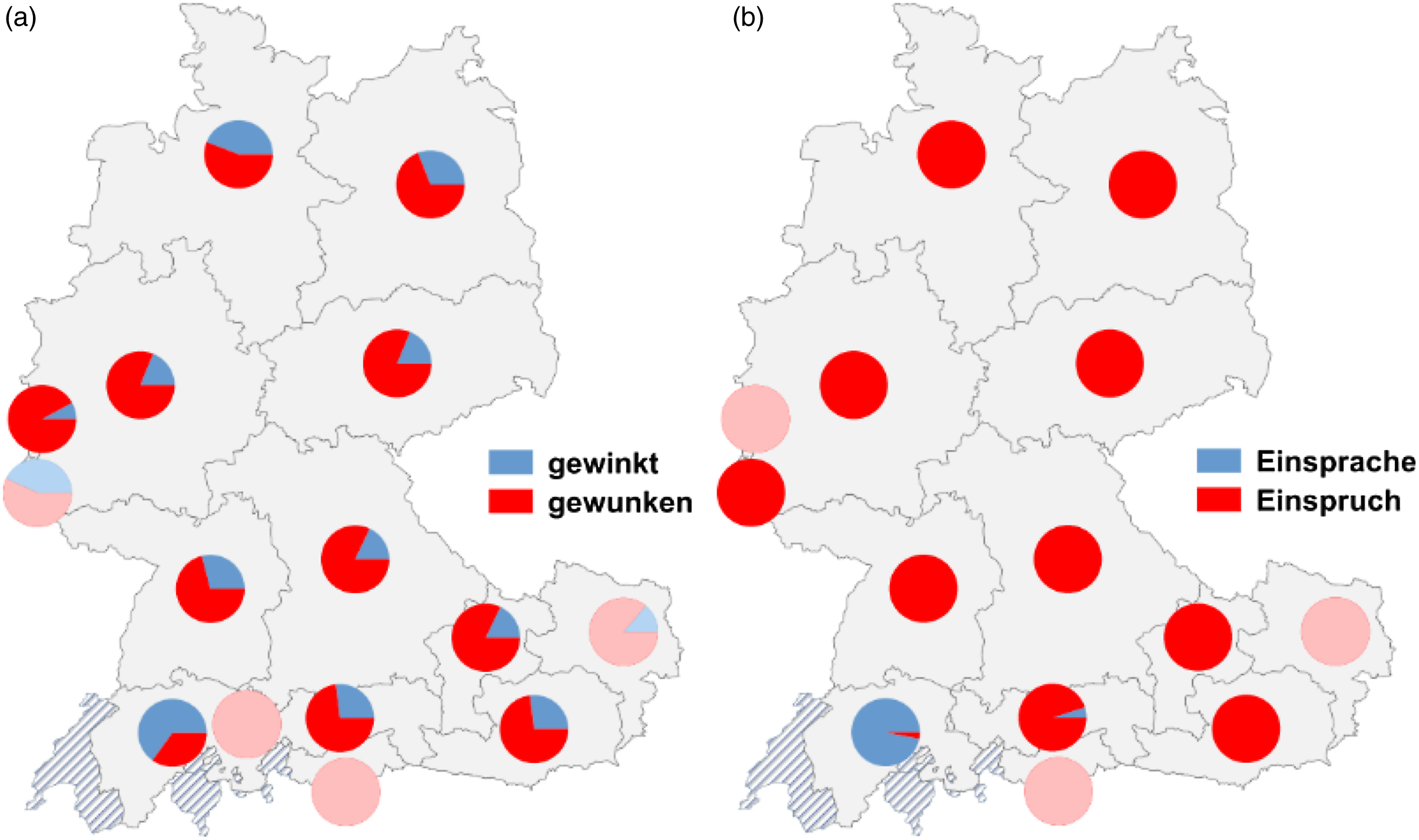
Map 3. Contradicting variant distributions. 3a (left): strong/weak participle inflection of winken ‘to wave’; 3b (right): differences in noun derivation of Einsprache versus Einspruch ‘objection.’
Against this background, an integrative analysis of all variables (bundles of functionally more or less equivalent variants) would be necessary to get an idea of the overall picture or to contribute to the discussion of relevant influencing factors. From an empirical perspective, it would be essential to aggregate the results in some way. On completion of the project, the corpus data as well as the statistical analyses were archived in a project-internal database so that the absolute and relative frequencies as well as the statistical results are available for further processing.
3. Spatial statistics for approaching standard variation
From a statistical point of view, there are a handful of tried and tested methods for abstracting more general tendencies from a certain quantity of individual instances. Regression models, for example, are increasingly used in linguistics as “a conceptually simple method for investigating functional relationships among variables” (Chatterjee, Hadi & Price, Reference Chatterjee, Hadi and Price2012:XIII). Applied to the case of standard variation, it is possible to define the single variant distributions (e.g., the relative frequencies) in a multiple logistic regression model as predictors and the defined areas as dependent variables to deduce their relation (“Variants a, b, c… are significant characteristics for the areas A, B, C…”). What is tested here are the relations between (dependent and independent) variables in a given dataset, which however does not address the question of establishing general tendencies in the sense of a varietal space: the areas are determined beforehand, they are not directly deduced from the data. Likewise, the frequently used t-test (bivariate) or the Analysis of Variance (ANOVA, multivariate) answer to the question of degrees of significance between predefined groups of variants. Those are ideal methods for answering research questions such as “Do speakers in area A use weak verbal inflection significantly more often than speakers in area B?” The distributional factors across areal borders, however, are not taken into consideration (see Rietveld & van Hout, Reference Rietveld and van Hout2005:1). For the purpose of the present study, alternative methods are better suited, methods that meet the following conditions: (1) the mathematical procedures are not based on predefined language areas (Rietveld & van Hout, Reference Rietveld and van Hout2005:49) as this is exactly what pluriareal concepts seek to avoid; and (2) the spatial dimension nevertheless must be one of the relevant influencing factors for estimating variant distributions. In section 3.1, statistical solutions for these demands are discussed, and section 3.2 describes the integration of spatial information in these methods. Section 4 contains the application of the proposed approaches to grammatical standard variation.
3.1 The search for similarities: Factor analysis and clustering
The need for automatically construing types or patterns has led to the development of a range of statistical analyses. Among the most commonly used are Factor Analysis (FA) and Clustering (CA). Footnote 8 FA is an approach for deriving one (or more) “synthetic,” not predefined independent variable(s) for the data. Footnote 9 Initially developed for research questions in psychology, its application in linguistics consists of comparing correlations of distributions of measured variables with the goal of construing one (or more) ideal “best-fit” distribution(s), correlating with most of the observed occurrences (Nerbonne, Reference Nerbonne2006). These so-called latent factors can explain most, yet not all, of the observed variances. For estimating general tendencies with regard to standard language variation, FA allows for the calculation of patterns of observed (measurable) variances. Explorative FA is usually carried out on the basis of a correlation matrix of all scores of instances followed by the elicitation of hypothetical factors, of “bundles” of correlating variant distributions. The optimal number of factors is not generally fixed but individually calculated by different methods, ranging from comparing the eigenvalue Footnote 10 to determining a number of factors in advance. The estimated factor loadings display the correlation between the generated factors and the measured variant distributions, which gives an indication of how “important” a factor is for the observed data. Footnote 11 In the specific case of grammatical variability, FA is used to generate groups of regions (factors) that show variability to a significant degree compared to an even distribution across the whole German-speaking area. It is crucial to note that the factors reflect the common variability in the data and not primarily the stable characteristics. For instance, when in the areas A and B, the dominating variant shows a relative frequency of 52%, and in the areas C and D, the same dominating variant shows a relative frequency of 98%. The first two areas could be ascribed to one factor, the second two to another. Still, it is important to notice that all four areas show the same dominating variant, hence the commonalities in fact exceed the variations. The relevance of this effect will be further discussed in section 3.3.
In the spatially influenced modification of Cluster Analysis applied here, the main goal is to aggregate those variant distributions that show similar characteristics. Clustering in general means to automatically unite patterns (or objects, depending on the research questions) that show a relative degree of homogeneity in comparison to the other defined groupings. One precondition of this method is to ensure the measurability of distance between the observed variants in order to set a numerical proximity measure. Among the most prevalently used is the Euclidian distance, the square root of the addition of squared differences of measures of every variant pair, hence the distance of two points in a two- or three-dimensional space. The next step in the analysis consists of choosing the algorithm (mostly partitioning or hierarchical methods) Footnote 12 by which the grouping of variants should be conducted (Backhaus et al., Reference Backhaus, Erichson, Plinke and Weiber2018:438). Comparing the defined distance measures, the algorithm of hierarchical agglomerative methods, for instance, successively combines the individual variants (beginning at the ones that show the smallest distance measures) until they are all united in one single group. The last step of clustering consists of deciding which number of clusters provides the “best” solution for the given research question. Widely used approaches for this assessment are the elbow-criterion (Scree-plot) or mathematical processes like the Stopping Rule method (Calinski & Harabasz, Reference Calinski and Harabasz1974). Rumpf et al. (Reference Rumpf, Simon Pickl, König and Schmidt2010:83) use a statistical method where the grouping of variants is stopped when the smallest distance between clusters exceeds a certain threshold, depending on the average of distance measured between two joined clusters (m), their variability (s) and the parameter k (= 1.7, Rumpf et al., Reference Rumpf, Simon Pickl, König and Schmidt2010:83). Under certain circumstances, however, it can also be useful to predefine a fixed number of clusters for approaching general tendencies (see section 4).
It will be shown below how FA and CA can produce important insights when applying them to the Variantengrammatik-project data: the evidence of general variability in the data, on the one hand, and the similarity of distribution patterns of dominating variants, on the other. Those are two different aspects of grammatical variation that should be assessed accordingly.
3.2 The spatial dimension
The recognition of space as one central factor involved in the variability of language is the pivot especially for dialectological studies. Footnote 13 In this field of research, the gathering of data has always gone hand in hand with its representation on geographical maps, showing variant distributions within a coherent language area (e.g. the German-speaking dialect regions). To abstract from singular maps or to establish relations between dialect areas, the aggregation of data was pursued, first and foremost by dialectometric methods (Nerbonne & Kretzschmar, Reference Nerbonne2006). In this field, the measuring of linguistic similarity and the integration of geographical distance in statistical estimations are seen as important parameters in defining a dialect space. Statistical methods allow for the quantitative description of variability, of continuous, merging distributions and fuzzy borders, in contrast to the mosaic of linguistically distinct areas with clear-cut borders often conceptualized in earlier studies (Francis, Reference Francis1983:158). With the aid of a symmetric matrix of locations (place × place), Goebl (Reference Goebl, Mattheier and Wiesinger1994, Reference Goebl2006) first determined the similarity between all points on a map, not only the relations between neighboring locations, resulting in a reduced data structure displaying similarities of lects. Those lects are not principally linked to a geographical region, only as a second step they are ascribed to a specific point in space (Goebl, Reference Goebl, Mattheier and Wiesinger1994:172). In contrast, more recent approaches in dialectometry view geographical locations as the central points of interest with variant distributions seen as the results of “spatial diffusion processes” (Pickl & Rumpf, Reference Pickl, Rumpf, Sandra Hansen, Stoeckle and Streck2012:207). The focus of these studies is not primarily the distribution of lects in space but the distribution of single variants in space (Pickl & Rumpf, Reference Pickl, Rumpf, Sandra Hansen, Stoeckle and Streck2012) with their joint analysis eventually supporting the assumption of generalized patterns. In the course of the pioneer research project New Dialectometry Using Methods from Stochastic Image Analysis (University of Augsburg and Ulm University), a bottom-up quantitative approach was elaborated that aggregates single variant distributions to establish interrelations between maps (Pickl & Rumpf, Reference Pickl and Rumpf2011, Reference Pickl, Rumpf, Sandra Hansen, Stoeckle and Streck2012; Pickl et al., Reference Pickl, Aaron Spettl, Elspaß, König and Schmidt2014; Rumpf et al., Reference Rumpf, Simon Pickl, König and Schmidt2009). Initially developed for and applied to dialectological research endeavors, the project’s basic methodology is suitable also for questions regarding standard variation, which is why its architecture is explained in further detail below. Footnote 14
Aiming at statistically revealing patterns that run through collected data, the first step is converting single distributions of variants into so-called area-class maps via intensity estimation. Footnote 15 This method rests on the assumption that linguistic distance/similarity is related to geographical distance/proximity: two identical variants are likely to belong to the same variant area, especially if they are located in neighboring locations. If they are distant to each other, or if a competing variant is also documented, their status as belonging to the same variant area is gradually weakened (Pickl & Rumpf, Reference Pickl, Rumpf, Sandra Hansen, Stoeckle and Streck2012:209). For every location of recording (see the dots in Map 4), the intensity estimates for each variant can be calculated from the share of a certain variant with regard to the frequencies of the alternative variant and with regard to the frequency of both in the surrounding area. Hence, the occurrence values for each variant (see quote) at a given location are set off against the occurrence values in the surrounding regions creating an intensity value for each location.

Map 4. Estimated intensities of perfect tense formation with haben (red) versus sein in the case of stehen (‘to stand’).
Each record location t is assigned an occurrence value l x (t) of the variant x: if x is the only variant occurring in the point-symbol map of location t, it is assigned the value l x (t) = 1. Otherwise, it is assigned its relative frequency of occurrence. For example, if x is one of three different variants occurring at location t, l x (t) = 1/3. Once a set of variant-occurrence maps is obtained from the raw data, a continuous intensity field is estimated for each variant-occurrence map. Informally speaking, at every location on the map, a variant’s intensity field indicates the likelihood of that variant occurring at the respective location (Rumpf et al., Reference Rumpf, Simon Pickl, König and Schmidt2009:6).
With this kernel estimation, Footnote 16 an intensity map for each variant can be generated, displaying the likelihood of its occurrence at any given location. This likelihood can be displayed by shaded area-maps (Voronoi-cells): varying colors are given to different variants of one variable, varying hues express varying degrees of likelihood for the respective variant. The richer the color the more dominant the variant in the specific area. A difference of color indicates a different dominating variant. Map 4 displays the calculated distributions of perfect formation with haben versus sein in the case of stehen (‘to stand’). The map clearly shows that in the north and in the mid-section of the German-speaking area, the dominant variant is the haben-perfect, whereas in large parts of the southern region, the sein-variant is apparently more frequent (with decreasing frequencies in the eastern regions of Switzerland and South Tyrol). Footnote 17
The estimated intensities, calculated for each and every variant, are the basic prerequisites for further stochastic analyses. Combining the estimated intensities of all recorded variants at all possible locations, the outcome should be an integrative area-class map, at best displaying a number of co-occurring variant patterns and their transition range. Applied to the question of grammatical standard variation in German and to the corresponding data basis, the graphical implementation of these results should directly display relevant standard varieties with regard to grammar and the course of possible borders. For this aggregation process, FA and CA are implemented in the GeoLing software.
4. Applying spatial statistics to the Variantengrammatik data
As explained above, the entries in the Handbook of Grammatical Variation in Standard German are based on data collected from sixty-eight newspapers evenly distributed over the coherent German-speaking area. This data is permanently saved in a project-internal database. The documents contain the plain search results, the statistical analyses and, vitally important for reconstructing the variants’ areal distributions, the relative frequencies of each and every observed variant in each of the eighteen predefined language areas (see section 2.2). One additional advantage of this specific database is that the relative frequencies are already checked for statistical significance, so that the exclusion of presumably accidental variant distributions was already performed in the course of the research project. For further analysis regarding spatial implications, however, the data has to be processed in two steps. First, the relevance of the predefined language areas needs to be abandoned, as any kind of spatial allocation should solely be the result of the data-driven analyses. Instead of language areas, the texts themselves, that is, the texts of the regional sections of the single newspapers, are defined as “informants.” Accordingly, the mailing addresses of the local newsrooms are roughly defined as record locations, occasionally also considering the respective newspaper’s distribution area. Footnote 18 As a second step in data processing, the relevant frequencies are converted to an Excel file with every line standing for a hypothetical informant’s answer. This is due to the fact that the GeoLing architecture is designed for a constant set of responses that emerges, for instance, from a dialectological questionnaire survey. As the relative frequencies were manually transformed into a fictional survey of one hundred “answers” per newspaper, for the time being, the analysis described in this paper is limited to the fields of verbal and nominal inflection and verbal and nominal word formation. Footnote 19 The missing-value-problem Footnote 20 leads to a limitation on variants with one or more alternative variant(s) per variable to avoid empty cells. In total, 92 variables (194 variant maps) were implemented for further processing.
For each of these variables, an intensity estimation (see section 3.2) and a corresponding area-class map can be generated. Apart from the graphical impression, the values of estimated intensities are displayed plus the statistical values of the maps’ compactness or the total border length (Rumpf et al., Reference Rumpf, Simon Pickl, König and Schmidt2010:76ff.). The example of Map 4, for instance (perfect tense formation with haben (red) versus sein in the case of stehen (‘to stand’), shows a variant border length of around 1,220 kilometers. Theoretically, if every point of measurement would show a different dominating variant than the neighboring areas, a border length of almost 10,000 kilometers would be possible; this speaks for a rather clear structure of areas in Map 4. The compactness of a map l¯ x explains which share of all variants is represented by assigning a point of location to a specific area as this aggregation process means to disregard the appearances of the nondominant variants. The occurrence value l x =1 would mean that at a given location only one variant x is documented, and no information gets lost when assigning it to the respective colored area. Occurrences of a competing variant y could lower the value of l x , if the location is ascribed to the area x, however, y will not be represented in the map. The overall compactness l¯ x of a map is the mean value of all variant occurrences for x at every location L¯ is the weighted mean of all l¯ x . In Map 4, for instance, the weighted mean L¯ = 0.8 indicates that the map represents 80% of the variable’s raw data. Footnote 21
Considering the individual maps, however, it is obvious that the definition of a general pattern in standard variation faces the exact same problem as noticed before and generally in quantitative studies: variants frequently show diverse geographical distributions (Grieve, Speelman & Geeraerts, Reference Grieve, Speelman and Geeraerts2011:202). In fact, there are a few maps where national borders seem to play a role in the variants’ occurrences (see Map 5a), others speak for the relevance of dialect regions (see Map 5b), and some do not display any obvious systematic segmentation (see Map 5c). Apart from this intuitive assessment, the application of statistical methods gives us a more reliable result.

Map 5. Distributions of the variables (a) Entscheid (blue) – Entscheidung (‘verdict’), (b) Werkstätte (red) – Werkstatt (‘garage’), and (c) preterite inflection of backen (backte (red) – buk) (‘to bake’).
Statistically speaking, varieties are regions ascribed to one common language but characterized by linguistic differences bigger than expected compared to an assumed homogeneous overall spatial variation (Pickl, Reference Pickl, Christen, Gilles and Purschke2017:263). To clarify if this is the case in our data, CA is applied to group similar variant distribution patterns. In the case of GeoLing, CA aggregates the maps themselves, hence the distribution patterns of the linguistic variables. It should be noted that this approach certainly deviates from the way CA is usually performed in dialectology where it clusters locations (see Leinonen, Çöltekin & Nerbonne, Reference Leinonen, Çölteki and Nerbonne2016), not distribution patterns. We are interested, however, in answering the question if the areal distributions of variants correlate, that is, if they show clusters of similar variation patterns. Instead of analyzing distributions of single variants, we search for similarities of variation patterns. To this end, hierarchical agglomerative clustering is applied to all implemented variables with the calculated relative intensities as distance measures between the maps and a standard normal distribution as the kernel function. The distance between clusters is set to complete linkage, Footnote 22 that is, the maximum of distances within one group is considered in the aggregation process (see section 2.1). For calculating the optimal bandwidth (for assessing the distance of influence for each record location), least-squares cross-validation (LSCV) is applied. This method finds a bandwidth that minimizes the mean squared difference of the calculated intensity estimate of a certain area from the observed intensity (Rumpf et al., Reference Rumpf, Simon Pickl, König and Schmidt2009:287). Footnote 23 As a threshold for stopping the clustering-process, k=1.7 is set in accordance with the program’s default value (Rumpf et al., Reference Rumpf, Simon Pickl, König and Schmidt2010:83), the clustering algorithm stops accordingly when the distance between clusters exceeds this level.
To support the idea of national varieties, CA should aggregate the maps of variant distributions (i.e., the estimated relative intensities of the single maps) according to, for instance, three clusters corresponding to the main centers: Austria, Germany, and Switzerland. This, however, is clearly not the case. The total of 92 analyzed variant distributions are aggregated to 85 clusters, hence most of the variant distributions are considered to be too different for being joined together. This may be seen as an effect of complete linkage: when focusing on the maximum of distances between already existing clusters and singular maps, the heterogeneous distributions (caused for instance by frequent outliers) may prevent the aggregation process. When inversely focusing on the average distances between maps, however, all maps are classified as belonging to the same single cluster. This effect suggests that the distributions in the data as a whole are too heterogeneous for reasonably assuming a general tendency. Strikingly, these results are repeated even when focusing on a smaller grammatical field such as verbal inflection or word formation. With complete linkage, the total of 58 variables of verbal inflection, for instance, are aggregated to fifty clusters, which shows that even within this limited grammatical area, most of the variant distributions are (at least in parts) too heterogeneous for deducing a common language area or variety. Footnote 24 The only area that shows slightly better results is nominal word formation. A total of 49 variables are aggregated to 18 clusters with the most comprehensive three groupings showing two comparatively homogeneous variant distribution patterns diffusing from (1) the southwest and (b) the southeast of the German-speaking area (see Maps 8 and 9). Note, however, that even in these cases, no clear correlation between the national border and the variant’s distribution can be deduced. Footnote 25 Rather, it seems conceivable that the dialect areas (see for instance Alemannic/Bavarian) play a role in the diffusion of variants in the standard language use, of course here too without the implication of clear-cut borders.
Just as the data-driven and mathematically calculated clustering does not support homogeneous language areas in the sense of varieties or national standard languages, the same must be assumed when predefining exactly three clusters, that is, when “forcing” the algorithm to aggregate three groups of (relative) similar distribution patterns. As Map 10 shows, the outcome is three clusters of, in each case, a few (two to eight) maps that in fact show alternating variants for certain areas, whereby here too national borders play a minor role. Besides the aforementioned areas of the southwestern and southeastern parts of the German-speaking area, cluster 4 displays general north-south differences that mainly concern the perfect tense formation (haben versus sein). The vast majority of distributions (72 variables out of 92) does not show alternating dominant variants but only differences in the distribution patterns of one and the same dominating variant. These differences occasionally might be explained roughly by the correlation with national borders. The maps clearly show, however, that the dominating variant usually stays the same (see Map 11). Footnote 26
As an intermediate result, we can say now that CA did not suggest clearly defined language varieties as the dominating variants. Rather, they seem to be evenly distributed across borders. Can we deduce from this result now that the coherent German language area is characterized by the use of a homogeneous German standard language? Probably not. As singular maps already have shown, there is variability in the data. To statistically approach this question, FA is applied to show if the nondominating component of grammatical variation significantly reveals areal tendencies. As discussed in section 3.1, the defined factors in FA are estimated vectors for correlating variances. Put simply, it calculates which factors best explain the differences in the data, a certain (and for each factor differing) degree of variability found in the analyzed data. Hence, subjecting the previously computed intensity maps to a FA should identify common spatial patterns of variability (Grieve, Speelman & Geeraerts, Reference Grieve, Speelman and Geeraerts2011). In contrast to CA implemented in GeoLing, FA aggregates singular variant distributions, not the estimated intensities. Thus, frequencies of alternating variants are not cumulated. The corresponding map of factors generated by GeoLing, comprising all of the implemented variants’ distributions, is displayed in Map 6. Here we see that the varying factors in fact show national tendencies, with the three generated areas explaining the recorded variability. The factor loadings in Table 1 illustrate the relevance of a location for a factor representing observed differences. We see that the share of explained variability is relatively high with an accumulated 78% for all three factors. The calculated factorial areas and the locations with the highest factor loadings (0.839 to 0.886) too are roughly representative for Germany (midwest), Austria (southeast), and Switzerland. This result indeed indicates the existence of statistically relevant grammatical variation considering the three biggest countries in the area under investigation. The observed variability of nation-specific grammatical variation, however, does not justify deducing standard varieties. Footnote 28 Such a conclusion would mean to blunder into the same trap as proponents of pluricentric approaches do on a more introspective-intuitive level: too much weight is given to differing variants while the largely existing linguistic homogeneity of consistent dominating variants is often ignored in the process. Map 7 underpins this argument. It illustrates three representative examples of variants that suggest the existence of three relevant factors, one for Austria, one for Germany, and one for Switzerland. The hues of the estimated relative intensities show, however, that the respective dominant variant is distributed more or less homogeneously over all of the German-speaking area. Accordingly, the factors are deduced predominantly by the decrease of relative frequency, not (only) by the occurrence of different dominating variants. Considering both the results from CA and FA, it is obvious that grammatical variability per se is a necessary but not sufficient precondition for assuming (national) standard varieties.

Map 6. Factor analysis resulting in three main factors (red-green-blue) roughly corresponding with national borders. (Underlying map: Google Maps 11.5.2021, maps.google.com)

Map 7. Distribution of (a) nominal inflection with -eur (versus -or), (b) genitive inflection with -es (versus -s), and (c) verbal inflection with -ieren (ersus -en).

Map 8. Cluster 4 of the variation patterns within nominal word formation: (a) word-formation with umlaut (i.e., Klassler/Klässler ‘pupil’), (b) diminutive-formation with –ler/-chen+umlaut (i.e., Tascherl/Täschchen ‘small bag’), and (c) word-formation with -er/-er+umlaut (i.e., Geher/Gänger ‘walker/goer’).

Map 9. Cluster 3 of the variation patterns within nominal word formation: (a) word-formation with -er/-ler+umlaut (i.e., Bezieher/Bezügler ‘recipient/subscriber’), (b) word-formation with Ø/-e (i.e., Limit/Limite ‘limit’ accompanied by gender differences), and (c) word-formation with Ø/-ung (i.e., Verlad/Verladung (‘loading/shipping’).

Map 10. Example distributions of three predefined clusters.

Map 11. Part of the variant distributions not aggregated to one of the three clusters of Map 11, in each case displaying one dominating variant.
Table 1. Explained variance, accumulated scores, and factor loadings for the three main factors displayed in Map 6.

5. Discussion
More than forty years after the first attempts of arguing for national varieties of German (Brandt & Freudenberg, Reference Brandt and Freudenberg1983:6; Clyne, Reference Clyne1984), solid corpus linguistic proof for these assumptions is still lacking. If we take the claim seriously that national varieties should systematically and significantly differ in at least all three core linguistic areas of phonology, grammar, and lexis (Dittmar & Schmidt-Regener, Reference Dittmar, Schmidt-Regener, Gerhard Helbig, Henrici and Krumm2001:521, differences in pragmatics are also often mentioned, see Berruto, Reference Berruto, Auer and Erich Schmidt2010:229; Schmidlin, Reference Schmidlin2011:85), the results of the present study neither support the idea of an uniform German standard language across borders, nor do they underpin the assumption of pluricentric varieties for German, as they do not confirm differences in the distribution of diverging—dominant!—grammatical variants. Footnote 29
The results of FA make it obvious that a careful interpretation of statistical methods is advisable. The conceptual difference between variable diffusion patterns of the same dominant variant on the one hand and the variable use of (nation-specific) variants on the other must be stressed for avoiding false conclusions. Focusing simply on differences between the estimated intensities, the existence of an alternative yet recessive variant b (that potentially could be nationally distributed) is displayed in FA by the further diminished occurrence of variant a. As a consequence, the factors display significant differences in distribution patterns, which, however, does not automatically reveal the areal specificity of alternating variants. The variation between different dominating variants, thus, is of secondary importance for calculating factors; it is, however, of primary importance for assuming nation-specific variants. Footnote 30 At the same time, the presented results of course do not speak for a homogeneous German standard language; they confirm regional, dialect-induced, or maybe even national differences that result from the existence of areal- or nation-specific secondary variants. Importantly, however, in most cases they are not competing with the supraregional variant predominantly used in the analyzed standard language settings. As mentioned before, FA reflects the intuition of assuming standard varieties as it captures lesser used, but at the same time, supposedly more salient language features. Variants different from what is perceived as one’s standard language use attract attention on the perception level. This alone, however, does not imply their linguistic dominance.
Similarly, the results of CA do not confirm the legitimacy of grouping together areal-specific distribution patterns, as they are evaluated as being too different. From the total of 92 analyzed variables, only 20 show alternating variants in the sense that there is a clear areal variability regarding the dominating variant. What is more, it has been shown that these areas by and large do not suggest significant correlations with national borders—at least, not all of them (see Map 10). Those 20 variables can be grouped together when determining a number of clusters in advance. Considering their comparatively rare occurrences, the significance of this endeavor seems doubtable. Generally speaking, CA confirms the assumed “Ein-Räumlichkeit” (Scheuringer, Reference Scheuringer1996:152) [‘one-spatiality,’ E.S./A.Z.] of the German variation space regarding dominating standard language variants.
One important remark must finally be made. The present paper puts aside the perceptional/cognitive dimension regarding the speakers themselves. Without discussing these emic approaches further at this point, it must be emphasized that the definition of a variety in perception linguistics is of fundamental difference to the one presented in the course of the present paper, supposedly leading to diverging and, in any case, noncomparable results (Maitz, Reference Maitz, Gilles, Scharloth and Ziegler2010:15). What is considered as being a variety on the one hand and what is practiced in real (standard) communication settings on the other are two different objects of research (Auer, Reference Auer2002, Reference Auer2004). The present study suggests that the mixing-up of these dimensions as well as hasty interpretations of statistical tests lead to conceptually grounded misunderstandings. When it is argued that quantitative corpus analysis and stochastics do not support the claim of national varieties, it is of course not to say that national varieties cannot be subjectively perceived by the speakers. It is simply not significantly displayed by their linguistic behavior.
Acknowledgments
The findings of this paper rest on data gathered and processed in the course of the research project Handbook of Grammatical Variation in Standard German (2011-2019), funded by Austrian Science Fund (FWF) I716-G18/I2067-G23, Deutsche Forschungsgemeinschaft (DFG) EL 500/3-1 and Schweizerischer Nationalfonds (SNF) 100015L_134895/156613). The authors acknowledge the financial support of the University of Graz.
Competing interests
The authors declare none.


 Open access