


1. Introduction
A dusty plasma is a complex plasma where the electrons are depleted onto the micrometre-sized and nanometre-sized dust grains, charging them negatively leaving the positive ions as dominant lighter charge carriers, in contrast to the electron–ion plasma where the electrons are the most mobile. We note that positively charged grains are also possible with sufficiently strong photo-ionisation. Dusty plasmas are common in laboratory experiments and astrophysical environments; examples range from the semiconductor industry to the Moon's surface, planetary ring systems, cometary tails, interstellar dust clouds and protoplanetary discs (Sagan & Khare Reference Sagan and Khare1979; Bliokh, Sinitsin & Yaroshenko Reference Bliokh, Sinitsin and Yaroshenko1995; Li & Mann Reference Li and Mann2012). In addition to gravity, drag and radiation pressure, they are highly affected by both the electric and magnetic fields (Horányi Reference Horányi1996; Shukla, Mendis & Chow Reference Shukla, Mendis and Chow1996). Therefore, the presence of the charged dust can modify various well-known physical processes in normal (non-dusty) plasmas such as turbulence (Tiwari et al. Reference Tiwari, Dharodi, Das, Patel and Kaw2015), wave modes propagation (Kotsarenko, Koshevaya & Kotsarenko Reference Kotsarenko, Koshevaya and Kotsarenko1998; Verheest Reference Verheest2001), electric conductivities in ionospheres (Shebanits et al. Reference Shebanits, Hadid, Cao, Morooka, Hunt, Dougherty, Wahlund, Waite and Müller-Wodarg2020) and the Enceladus plume (Yaroshenko & Lühr Reference Yaroshenko and Lühr2016; Simon et al. Reference Simon, Saur, Kriegel, Neubauer, Motschmann and Dougherty2011) and ambipolar diffusion (or ambipolar drift) (Amiranashvili & Yu Reference Amiranashvili and Yu2002). Ambipolar diffusion is a unique phenomena for plasmas that forms as a direct consequence of charge imbalance caused by the fast motion of the more mobile particles and the tendency of the plasma to remain neutral on spatial scales larger than a Debye length. For collisionless space plasmas, it plays an essential role in the transport of the charged particles and in regulating the star formation rate (Li & Mann Reference Li and Mann2012). Despite the increasing scientific interest of dusty plasmas in the last 40 years, the effect of the nanometre-sized charged dust on the ambipolar diffusion process in our solar system has not been studied in situ. In this work we address this topic in Saturn's environment, as it offers a unique opportunity with its dusty rings and the availability of Cassini's in situ data, in particular from the Radio and Plasma Waves Science (RPWS) instrument.
In the rapidly corotating magnetosphere of Saturn (Sittler et al. Reference Sittler, Thomsen, Johnson, Hartle, Burger, Chornay, Shappirio, Simpson, Smith and Coates2006), the gravitational and centrifugal forces play a major role in the distribution of the charged particles along the magnetic field lines, particularly in the presence of heavy ions such as oxygen ions (such as $\text {O}_{2}^+$ and $\text {O}^+$
 ). Along the field lines, the effect of the centrifugal force increases outward from Saturn, and confines the ions near the equatorial plane creating a plasma sheet-like structure, whereas the effect of the gravitational force increases inwards and pulls them back into Saturn (Northrop & Hill Reference Northrop and Hill1982, Reference Northrop and Hill1983). Due to a large mass difference between the electrons and ions, the centrifugal force causes a slight charge separation between them. This creates a polarisation electrostatic field along the magnetic field lines (hereafter, parallel electrostatic field, $\boldsymbol {E}_{\parallel }$
 ) that acts to preserve quasi-neutrality on a larger scale (Persson Reference Persson1963). As a consequence, under the effect of $\boldsymbol {E}_{\parallel }$
 , the ions and the electrons remain coupled to each other and diffuse together as a single fluid. Since the Voyager era, ambipolar diffusion has been identified as one of the main processes that governs the behaviour of the plasma along the magnetic field lines in the inner magnetosphere of Saturn and various plasma density models were developed to map the distribution of the electrons and ions in the planet's magnetosphere (Wilson & Waite Reference Wilson and Waite1989; Richardson & Sittler Reference Richardson and Sittler1990; Maurice et al. Reference Maurice, Blanc, Prangé and Sittler1997; Richardson & Jurac Reference Richardson and Jurac2004; Persoon et al. Reference Persoon, Gurnett, Santolik, Kurth, Faden, Groene, Lewis, Coates, Wilson and Tokar2009). Using multi-component simulations, Maurice et al. (Reference Maurice, Blanc, Prangé and Sittler1997) estimated $\lVert \boldsymbol {E}_{\parallel } \rVert$
 and investigated its effect on the distribution of the plasma particles along the field lines up to 20 $\text {R}_{s}$
 . They showed that $\lVert \boldsymbol {E}_{\parallel } \rVert$
 increases with distance from the planet because of the increase of the centrifugal force, and reaches a maximum value of the order of $10^{-7} \, \text {V}\, \text {m}^{-1}$
 around $7.5 \, \text {R}_{s}$
 between latitudes of approximately $4^{\circ }$
 and $11^{\circ }$
 . Moreover, they showed that the light ions ($\text {H}^+$
 ) are redistributed by the electrostatic field and float off the equator, whereas the heavier particles ($\text {O}^+$
 ) are confined at the equator. More complete and detailed characterisation of the spatial distribution of the electrons and ions at Saturn's equatorial regions were possible after the entry of the Cassini–Huygens spacecraft into orbit around Saturn (SOI) in July 2004. Persoon et al. (Reference Persoon, Gurnett, Santolik, Kurth, Faden, Groene, Lewis, Coates, Wilson and Tokar2009) used a diffusive equilibrium model to describe the distribution of the water group ions, protons, and electrons in the E ring region (between 3.6 $\text {R}_{s}$
 and 10 $\text {R}_{s}$
 ), by determining the equatorial ions densities and investigating the relative importance of the different terms in the force balance equation. Their model showed that for equatorial latitudes ${\lesssim }20^\circ$
 and L-shells ${\lesssim }5 \, \text {R}_{s}$
 , the distribution of the protons peaks above the ring plane, as a consequence of the significant importance of the ambipolar force. However, the heavier ions were shown to be confined to the ring plane as they are mostly affected by the centrifugal force (in agreement with Maurice et al. Reference Maurice, Blanc, Prangé and Sittler1997). Similar behaviour of the ions were also showed by Sittler et al. (Reference Sittler, Thomsen, Johnson, Hartle, Burger, Chornay, Shappirio, Simpson, Smith and Coates2006, Reference Sittler, Andre, Blanc, Burger, Johnson, Coates, Rymer, Reisenfeld, Thomsen and Persoon2008) using the in situ Cassini Plasma Spectrometer (CAPS) data. In addition to the E ring, ambipolar diffusion has been identified as one of the key driving processes along the main rings-connecting flux tubes. Using the in situ RPWS data and thanks to Cassini's final proximal orbits, Farrell et al. (Reference Farrell, Hadid, Morooka, Kurth, Wahlund, MacDowall, Sulaiman, Persoon and Gurnett2018) demonstrated the presence of strong ambipolar forces that draw out the cold ionospheric plasma along the field lines to replenish the flux tubes connected to the A and B rings. These findings were consistent with the presence of the ring-plasma cavity feature observed during SOI at the footprint of the same field lines close to the main rings (Farrell et al. Reference Farrell, Kurth, Gurnett, Persoon and MacDowall2017). Although these different studies have revealed the important role of the ambipolar electrostatic field in the magnetosphere of Saturn, the presence of the charged dust particles, with low charge-to-mass ratio, and their effect on the ambipolar diffusion process remain open questions.
The Cassini particle instruments have confirmed that the E ring consists of neutrals, plasma and predominantly negatively charged nanometre-sized dust grains (Jones et al. Reference Jones, Arridge, Coates, Lewis, Kanani, Wellbrock, Young, Crary, Tokar and Wilson2009; Wahlund et al. Reference Wahlund, André, Eriksson, Lundberg, Morooka, Shafiq, Averkamp, Gurnett, Hospodarsky and Kurth2009; Morooka et al. Reference Morooka, Wahlund, Eriksson, Farrell, Gurnett, Kurth, Persoon, Shafiq, André and Holmberg2011; Hill et al. Reference Hill, Thomsen, Tokar, Coates, Lewis, Young, Crary, Baragiola, Johnson and Dong2012) that originate from the southern pole exhaust plumes on Enceladus (Jones et al. Reference Jones, Arridge, Coates, Lewis, Kanani, Wellbrock, Young, Crary, Tokar and Wilson2009). Other diffuse rings of Saturn include the F, Janus and Epimetheus rings. They are populated with dust particles and located at the outer edge of the main rings around 2.5 $\text {R}_{s}$ close to the orbits of Janus and Epimetheus moons. The Cassini spacecraft had the special opportunity to investigate this dusty region using both remote sensing and in situ measurements during the 20 near-polar ‘ring-grazing’ orbits that crossed the ring plane at a distance of approximately $2.5 \, \text {R}_{s}$
 between 30 November 2016 and 22 April 2017. The Wide Band Receiver of the RPWS instrument and the Cosmic Dust Analyzer (CDA) high-rate detector could provide direct measurements of the micrometre-sized dust densities and distribution (Ye et al. Reference Ye, Kurth, Hospodarsky, Persoon, Gurnett, Morooka, Wahlund, Hsu, Seiß and Srama2018). Furthermore, from the difference of the electron and ion densities measured by the Langmuir Probe (LP), part of the RPWS consortium, the number densities of the micrometre- and sub-micrometre-sized dust could be inferred by Morooka et al. (Reference Morooka, Wahlund, Andrews, Persoon, Ye, Kurth, Gurnett and Farrell2018). They showed that Janus and Epimitheus rings are dominated by negatively charged nanometre-sized grains (and/for negative cluster ions) up to approximately $0.1\, \text {R}_{s}$
 in the vertical direction from the ring plane ($Z$
 ). A core layer of micrometre-sized dust was also evidenced to be confined in a very narrow region ($\vert \text {Z} \vert \leq 0.02 \, \text {R}_{s}$
 ). It is worth noting that in this region, close to Saturn's F ring, the dusty plasma condition is satisfied. This condition is such that $a_d \ll d \ll \lambda _D$
 , where $a_d$
 , $d$
, $d$ and $\lambda _D$
 are the typical grain radius, the inter-grain distance and the dust Debye length, respectively (Shukla & Mamun Reference Shukla and Mamun2002). Therefore, the ions, electrons and the nanometre-sized charged dust can be considered as a collective dusty plasma ensemble and play an important role in plasma dynamics in Saturn's rings. In fact, electrostatic coupling of micrometre-sized dust with the plasma is thought to be responsible for the ‘spokes’ formation by rapid transport or levitation of the charged dust in the visible inner rings (Smith et al. Reference Smith, Soderblom, Beebe, Boyce, Briggs, Bunker, Collins, Hansen, Johnson and Mitchell1981; Hill & Mendis Reference Hill and Mendis1982; Goertz Reference Goertz1984; Goertz et al. Reference Goertz, Morfill, Ip and Havnes1986; Horányi et al. Reference Horányi, Hartquist, Havnes, Mendis and Morfill2004).
In this paper, we study the effect of the negatively charged nanometre-sized grains on the ambipolar diffusion process, by focusing on the RPWS/LP data during the F-ring-grazing orbits that were analysed by Morooka et al. (Reference Morooka, Wahlund, Andrews, Persoon, Ye, Kurth, Gurnett and Farrell2018). In addition to the RPWS/LP data we also use the magnetic field data from the MAG instrument (Dougherty et al. Reference Dougherty, Kellock, Southwood, Balogh, Smith, Tsurutani, Gerlach, Glassmeier, Gleim and Russell2002). We divide this work into two parts, theoretical and data analysis. First, in § 2, we derive a general expression of $\boldsymbol {E}_{\parallel }$ in the presence of negatively charged dust. Then, in § 3, we briefly explain the measurement principles of the LP and describe the methodology we use in this study. In § 4, we estimate $\lVert \boldsymbol {E}_{\parallel }\rVert$
 based on the LP and MAG data and compare the relative importance of the different terms in the force balance equation. Finally, in §§ 5 and 6, we discuss and conclude the different results.
2. Polarisation electrostatic field and ambipolar diffusion
Assuming a partially ionised plasma corotating with a planetary magnetosphere, the general momentum balance equation for charged particles is given by (Schunk & Nagy Reference Schunk and Nagy2009)

where for a fluid of species $s$ , the left-hand side is the sum of the local and convective motion terms, and the right-hand side is the sum of acting forces: the net force imposed by the pressure gradient, the Lorentz force, the gravitational and inertial forces, the drag force and the magnetic mirror force, respectively. We note that the heat flow, stress and all higher-order moments are being neglected. The bulk velocity, pressure, number density, the mass and the charge number of the species $s$
 are denoted by $\boldsymbol {u}_{s}$
 , $p_s$
 , $n_s$
 , $m_s$
 and $z_s$
 , respectively. Here $\nu _{st}$
 is the momentum transfer collision frequency between a source species $s$
 and target species $t$
 , and $\boldsymbol E$
 and $\boldsymbol B$
 denote the electric and magnetic fields, respectively, and $\mu _s=mv_{s\perp }^2/2B$
 . The sum of the gravitational, centrifugal and coriolis acceleration is $\boldsymbol {G}= \boldsymbol {g}-{\boldsymbol \omega _s}\times ({\boldsymbol \omega _s} \times \boldsymbol {r})-2 {\boldsymbol \omega _s}\times \boldsymbol {u}$
 , where $\boldsymbol \omega _s$
 is the angular velocity of the species $s$
 and $\boldsymbol r$
 the position vector from the rotation axis of the planet. Considering Saturn's magnetosphere, as the motion of the particles along $\boldsymbol {B}$
 close to the equatorial plane is almost parallel to the rotation axis of Saturn, one can neglect the coriolis force. Moreover, considering spherical coordinates, for a particle located around Saturn, the gravitational acceleration vector is given by $\boldsymbol {g}=-g \boldsymbol {\hat e_r}$
 (where $g\approx 3.8 \times 10^{16}r^{-2}$
 m s$^{-2}$
 ) and the centrifugal acceleration vector by ${\boldsymbol \omega _s}\times ({\boldsymbol \omega _s} \times \boldsymbol {r})= r{\omega }^2 \cos ^2 \theta \boldsymbol {\hat e_r} + r{\omega }^2 \cos \theta \sin {\theta } \boldsymbol {\hat e_\theta }$
 , where $\theta$
 is the elevation angle and $r$
 is the radial distance from the centre of the planet. We assume the ions’ and electrons’ co-rotation angular velocity to be the same as Saturn's angular velocity $(\omega _S \approx 1.66 \times 10^{-4}$
 rad s$^{-1}$
 ) and the dust to have an orbital angular velocity.
We consider a three-component collisional dusty plasma consisting of electrons, singly and positively charged ions and negatively charged dust particles ($q_d < 0$ with $q_d = -q_ez_d$
 ), embedded in a strongly magnetised environment where the $\boldsymbol {B}$
 field is nearly vertical. For convenience, we also consider a dominant neutral species $(n)$
 . Moreover, we assume zero current (one ensemble of dusty plasma), diffusive equilibrium (subsonic, $\boldsymbol {u}_s \boldsymbol {\cdot } \boldsymbol {\nabla } \boldsymbol {u}_s \rightarrow 0$
 and slowly varying flow, ${\partial }/{\partial t} \rightarrow 0$
 ), and the motion parallel to the $\boldsymbol {B}$
 field ($\boldsymbol {u}_s\times \boldsymbol {B} \rightarrow 0$
 ). Following these assumptions, the momentum balance equation (2.1) for the ions $(i)$
 , electrons $(e)$
 and dust $(d)$
 reduces to

where $\boldsymbol {E}_{\parallel }$ is the parallel polarisation electrostatic field that develops because of the slight separation between two oppositely charged particles in the presence of charged dust, and $\nu _{id}$
 represents the Coulomb collision frequency, $\nu _{in}$
 the elastic collision frequency and $\nu _{dn}$
 the hard-sphere collision frequency. The expressions of the collision frequencies are given in appendix A. We note that in this particular case study, the use of the magnetic mirror force is valid, as both the protons and dust gyroradius ($\rho _{iL}$
 and $\rho _{dL}$
 , respectively) are much smaller than the length scales of the magnetic field variations ($1/\rho _{iL} \sim 10^{-2}$
 m$^{-1}$
 and $1/\rho _{dL} \sim 10^{-3}\,\textrm {m}^{-1}\gg \boldsymbol {\nabla }_{\parallel }B/B \sim 10^{-10}\,\textrm {m}^{-1}$
 ).
).
To obtain a general expression of $\boldsymbol {E}_{\parallel }$ , we solve $(i)-(e)-(d)$
 . Using the charge neutrality condition in the dominance of negatively charged grains ($n_i=n_e+z_d n_d$
 ) and the fact that $n_sm_s\nu _{st}=n_t m_t\nu _{ts}$
 (Schunk & Nagy Reference Schunk and Nagy2009), $\boldsymbol {E}_{\parallel }$
 becomes

Neglecting the terms that contain $m_e$ ($m_e \ll m_i,m_d$
 ):
):

For case studies where the contribution of the neutrals and the magnetic mirror forces are negligible (see the discussion in § 5), one obtains a reduced form of $\boldsymbol {E}_{\parallel }$ :
:

Note that in the absence of dust, (2.5) reduces to the classical expression of the polarisation electrostatic field (Schunk & Nagy Reference Schunk and Nagy2009):

3. Measurement principles and methodology
3.1. Ions and electrons parameters
The ions and electrons parameters are inferred from the sweep mode of the Langmuir probe, one of the main components of Cassini's RPWS consortium (Gurnett et al. Reference Gurnett, Kurth, Kirchner, Hospodarsky, Averkamp, Zarka, Lecacheux, Manning, Roux and Canu2004). The 5 cm spherical probe is mounted on an approximately $1.5 \, \textrm {m}$ boom and measures the current of the charged particles in two different modes, the voltage sweep mode and a high-resolution 20 Hz continuous mode (Gurnett et al. Reference Gurnett, Kurth, Kirchner, Hospodarsky, Averkamp, Zarka, Lecacheux, Manning, Roux and Canu2004). During the sweep mode, and for the considered ring-grazing orbits, the probe measures the plasma current across the bias voltage interval of ${\pm }$
 32 V every 48 s. From the current–voltage curve it is possible to derive the electron ($n_e$
 ) and ion densities ($n_i$
 ) as well as the electron temperatures ($T_e$
 ) and the spacecraft potential ($U_{sc}$
 ) (Fahleson Reference Fahleson1967; Wahlund et al. Reference Wahlund, André, Eriksson, Lundberg, Morooka, Shafiq, Averkamp, Gurnett, Hospodarsky and Kurth2009; Morooka et al. Reference Morooka, Wahlund, Eriksson, Farrell, Gurnett, Kurth, Persoon, Shafiq, André and Holmberg2011; Holmberg et al. Reference Holmberg, Wahlund, Morooka and Persoon2012; Shebanits et al. Reference Shebanits, Wahlund, Edberg, Crary, Wellbrock, Andrews, Vigren, Desai, Coates and Mandt2016; Holmberg et al. Reference Holmberg, Shebanits, Wahlund, Morooka, Vigren, André, Garnier, Persoon, Génot and Gilbert2017).
3.2. Dust parameters
None of the Cassini particles instruments was designed to directly measure sub-micrometre charged grains. The CDA could only detect particles of radii $a \gtrsim 1 \, \mathrm {\mu }$ m (Srama et al. Reference Srama, Kempf, Moragas-Klostermeyer, Helfert, Ahrens, Altobelli, Auer, Beckmann, Bradley and Burton2006; Kempf et al. Reference Kempf, Beckmann, Moragas-Klostermeyer, Postberg, Srama, Economou, Schmidt, Spahn and Grün2008), and the RPWS electric antennae were only sensitive to charged grains larger than a few micrometres (Gurnett et al. Reference Gurnett, Kurth, Kirchner, Hospodarsky, Averkamp, Zarka, Lecacheux, Manning, Roux and Canu2004; Ye et al. Reference Ye, Gurnett, Kurth, Averkamp, Kempf, Hsu, Srama and Grün2014; Ye, Gurnett & Kurth Reference Ye, Gurnett and Kurth2016; Ye et al. Reference Ye, Kurth, Hospodarsky, Persoon, Gurnett, Morooka, Wahlund, Hsu, Seiß and Srama2018). Nevertheless, due to the absorption of the electrons by all the grains, including the nanoparticles, the existence of the nanometre-sized grains and their total charge densities ($z_dn_d$
 ) can be inferred directly from the LP-derived ion and electron densities as $z_dn_d = n_i-n_e$
 as a consequence from the charge neutrality (Wahlund et al. Reference Wahlund, André, Eriksson, Lundberg, Morooka, Shafiq, Averkamp, Gurnett, Hospodarsky and Kurth2009; Shafiq et al. Reference Shafiq, Wahlund, Morooka, Kurth and Farrell2011; Shebanits et al. Reference Shebanits, Wahlund, Mandt, Ågren, Edberg and Waite2013; Engelhardt et al. Reference Engelhardt, Wahlund, Andrews, Eriksson, Ye, Kurth, Gurnett, Morooka, Farrell and Dougherty2015; Shebanits et al. Reference Shebanits, Wahlund, Edberg, Crary, Wellbrock, Andrews, Vigren, Desai, Coates and Mandt2016; Morooka et al. Reference Morooka, Wahlund, Andrews, Persoon, Ye, Kurth, Gurnett and Farrell2018, Reference Morooka, Wahlund, Hadid, Eriksson, Edberg, Vigren, Andrews, Persoon, Kurth and Gurnett2019). The general expression for the total dust density ($n_d$
 ) of radius $a$
 can be obtained from a power law differential size distribution of the dust (Yaroshenko et al. Reference Yaroshenko, Ratynskaia, Olson, Brenning, Wahlund, Morooka, Kurth, Gurnett and Morfill2009):

where $a$ is the size of the grain in the interval [$a_\textrm {min},a_\textrm {max}$
 ], $\mu$
 is the power law index and $K$
 is a normalisation constant. Then $n_d$
 is given by

where $q_e$ is the elementary charge, $\epsilon _0$
 the vacuum permittivity and

Assuming a spherical shape for the dust particles, and considering that water ice grains are dominant in Saturn's rings (mass density of the water ice, $\rho =920 \, \textrm {kg}\,\textrm {m}^{-3}$ ), the mass density of the dust particles of radius ranging from $a_\textrm {min}$
 to $a_\textrm {max}$
 , can be estimated as

3.3. Method
Using the ions, electrons and dust parameters inferred from the RPWS/LP measurements (Morooka et al. Reference Morooka, Wahlund, Andrews, Persoon, Ye, Kurth, Gurnett and Farrell2018), and assuming a negligible contribution of the neutrals and the magnetic mirror forces (see the discussion in § 5), we quantify the polarisationelectrostatic field in the presence ($\boldsymbol {E}_{\parallel }$ ) and absence ($\boldsymbol {E}^{\prime }_{\parallel }$
 ) of dust from (2.5) and (2.6), respectively, and investigate the contribution of the different forces: the pressure gradient ($\boldsymbol {E}_{\parallel p}$
 ), gravitational ($\boldsymbol {E}_{\parallel g}$
 ) and the centrifugal ($\boldsymbol {E}_{\parallel \textrm {cf}}$
 ) force. As measurements of the ion and dust velocities were not available during the F-ring-grazing orbits, we first neglect the ion–dust drag force ($\boldsymbol {E}_{\parallel \Delta u_{id}}=n_im_i\nu _{id}(\boldsymbol {u}_i-\boldsymbol {u}_d)_{\parallel }/2q_en_i$
 ) and then discuss its contribution in § 5. We note that the parallel component of the electrostatic field is obtained by projecting the different terms on the magnetic field data measured by the MAG instrument. For convenience, we rewrite $\boldsymbol {E_{\parallel }}$
 as
as

where

Similarly, $\boldsymbol {E^\prime _{\parallel }}$ is written as

where

We use the plasma parameters inferred directly from the LP: $n_e$ , $n_{i}$
 , $n_d$
 and $T_e$
 and consider the presence of the dominant ions ($\textrm {O}_{2}^+$
 and $\textrm {H}_{2}^+$
 ) near the F ring (Tseng, Johnson & Elrod Reference Tseng, Johnson and Elrod2013). For the ion temperature ($T_i$
 ), we assume the temperature of the water group ions inside the dusty region ($-0.12 \, \textrm {R}_{s} < \textrm {Z} < 0.11\, \textrm {R}_{s}$
 ) and the proton temperature outside, using $T_{\textrm {W}^+}=0.22*(L/4)^{2.5}$
 and $T_{\textrm {H}^+}=3.5*(L/4)^{2}$
 , respectively, from (Sittler et al. Reference Sittler, Thomsen, Johnson, Hartle, Burger, Chornay, Shappirio, Simpson, Smith and Coates2006). The average ion mass of the dominant ion species ions is calculated as

using the modelled ion densities by Tseng et al. (Reference Tseng, Johnson and Elrod2013). On average, we have $m_i \sim 29 \, \textrm {amu}$ , $T_{H^+} \sim 0.07 \, \textrm {eV}$
 and $T_{W^+} \sim 1.4 \, \textrm {eV}$
 . There was no measurements of the dust temperature ($T_d$
 ) in the F ring region. However, because the F ring and the Cassini Division (CD) have similar optical depth values ($\tau \sim 0.1$
 ), we assume that $T_d \sim T_{F} \sim T_{CD} \sim 88\, \textrm {K}$
 as observed by the Composite Infrared Spectrometer (CIRS) during the ring-grazing orbits of Cassini (Tiscareno et al. Reference Tiscareno, Nicholson, Cuzzi, Spilker, Murray, Hedman, Colwell, Burns, Brooks and Clark2019).
4. Data analysis: Cassini's F-ring-grazing orbits
4.1. RPWS/LP data
Using the data collected by the RPWS/LP instrument (§ 3) during Cassini's F-ring-grazing orbits, we focus the analysis on the near-equatorial plane ($\vert \textrm {Z} \vert \lesssim 0.4\, \textrm {R}_{s}$ , latitude $< 10^{\circ }$
 ) and select the cases for which the inferred ion and electron density profiles were smooth (absence of large fluctuations) and were converging to similar values (as expected from quasi-neutrality for $\vert \textrm {Z} \vert \gtrsim 0.1\, \textrm {R}_{s}$
 ). This constraint leads to five orbits: revs 253, 254, 266, 267 and 268.
In figure 1, we show the plasma data for rev 254 that has been discussed in detail in Morooka et al. (Reference Morooka, Wahlund, Andrews, Persoon, Ye, Kurth, Gurnett and Farrell2018). In figure 1(a), the green and blue curves represent the ion ($n_i$ ) and electron ($n_e$
 ) LP-derived charge densities, respectively, plotted versus the vertical distance ($\textrm {Z}$
 ) from the ring plane. Briefly summarising the observations from (Morooka et al. Reference Morooka, Wahlund, Andrews, Persoon, Ye, Kurth, Gurnett and Farrell2018), one can see that, away from the equator ($\vert \textrm {Z} \vert \gtrsim 0.1\, \textrm {R}_{s}$
 ), the electron and ion number densities are very comparable and increase gradually for decreasing $\textrm {Z}$
 . A clear difference between $n_i$
 and $n_e$
 , with $n_e < n_i$
 , can be noted close to Saturn's equatorial plane between around $-0.12 \, \textrm {R}_{s} < \textrm {Z} < 0.11\, \textrm {R}_{s}$
 (grey shaded area), where $n_i$
 increases sharply to approximately $200 \, \textrm {cm}^{-3}$
 whereas $n_e$
 remains lower at approximately $50 \, \textrm {cm}^{-3}$
 . The authors have shown that this deficiency in the electron number density was caused by the dominance of the negatively charged nanometre-sized grains in this region ($\vert \textrm {Z} \vert \lesssim 0.1\, \textrm {R}_{s}$
 ) with a total charged dust density ($n_d$
 ) of approximately $100\, \textrm {cm}^{-3}$
 . The dust number density inferred from the LP measurements is represented by the solid red curve. Using the same parameters as in Morooka et al. (Reference Morooka, Wahlund, Andrews, Persoon, Ye, Kurth, Gurnett and Farrell2018), $n_d$
 is computed from (3.2) for a dust particle of radius $a$
 varying from $a_\textrm {min}=1 \, \textrm {nm}$
 to $a_\textrm {max}=100 \, \textrm {nm}$
 and a power law distribution index $\mu =5$
 (see Morooka et al. (Reference Morooka, Wahlund, Andrews, Persoon, Ye, Kurth, Gurnett and Farrell2018) for more details). The data in dashed lines are calculated assuming an exponential decay of the dust densities, $n_d=n_{d0}\exp (-\textrm {Z}/\textrm {H})^2$
 , where $n_{d0}$
 represents the charged dust number density for $\textrm {Z}=0$
 and $\textrm {H}=0.054 \, \textrm {R}_{s}$
 is the estimated scale height of the nanometre-sized grains (Morooka et al. Reference Morooka, Wahlund, Andrews, Persoon, Ye, Kurth, Gurnett and Farrell2018). In the absence of dust ($\vert \textrm {Z} \vert \gtrsim 0.1\, \textrm {R}_{s}$
 ), the plasma is quasi-neutral and the measured difference between $n_e$
 and $n_i$
 is due to the low signal-to-noise ratio of the LP in this region, where the plasma density ($\sim 10 \, \textrm {cm}^{-3}$
 ) approaches the measurement limits of the LP (Morooka et al. Reference Morooka, Wahlund, Andrews, Persoon, Ye, Kurth, Gurnett and Farrell2018). Therefore, to avoid numerical errors from the noise in the derivation of $\boldsymbol {E_{\|}}$
 , we strictly enforce the quasi-neutrality, approximating the ion densities to be equal to the electron densities for $\vert \textrm {Z} \vert \gtrsim 0.1\, \textrm {R}_{s}$
 . These approximated ion densities ($n_{i,\,approx}$
 ) are represented by the dashed yellow line. The modelled dominant molecular hydrogen and oxygen ion and neutral densities (Tseng et al. Reference Tseng, Johnson and Elrod2013) are given in figure 1(b) for reference. As expected, the neutral densities dominate close to the ring plane. In particular, $n_{\textrm {H}_{2}}$
 reaches a maximum value of approximately $10^3 \, \textrm {cm}^{-3}$
 , about one order of magnitude larger than the oxygen ion ($n_{\textrm {O}_{2}^+}$
 ) densities. The electron temperature ($T_e$
 , figure 1(c)) increases from approximately $0.5 \, \textrm {eV}$
 to approximately $2 \, \textrm {eV}$
 away from the equatorial plane, due to convection. The local increase at the equator is attributed to the presence of the negatively charged dust that induces electron heating in their potential well (Farrell et al. Reference Farrell, Kurth, Gurnett, Persoon and MacDowall2017; Morooka et al. Reference Morooka, Wahlund, Andrews, Persoon, Ye, Kurth, Gurnett and Farrell2018).

Figure 1. Plasma parameters for rev 254 versus the vertical distance from the ring plane ($\textrm {Z}$ ). (a) The LP-derived number density of the electrons ($n_e$
 ) is shown in blue and the ions ($n_i$
 ) in green. In order to enforce quasi-neutrality outside the dusty region, we set $n_i=n_e$
 for $\vert \textrm {Z} \vert \gtrsim 0.1\, \textrm {R}_{s}$
 shown in yellow dashed line as the approximated ion density ($n_{i,\,\textrm {approx}}$
 ). The total dust densities ($n_d$
 , solid red line) is computed from (3.2) for a nanometre-sized particle of size $a$
 varying from $a_\textrm {min}=1 \, \textrm {nm}$
 to $a_\textrm {max}=100 \, \textrm {nm}$
 and a power law index $\mu =5$
 . For $\vert \textrm {Z} \vert > 0.1\, \textrm {R}_{s}$
 (dashed red line), $n_d$
 is calculated assuming an exponential decay with a scale height value $\textrm {H}=0.054\,\textrm {R}_{s}$
 . (b) The modelled ions ($\textrm {O}_{2}^+$
 , $\textrm {H}_{2}^+$
 ) and neutral ($\textrm {O}_{2}$
 , $\textrm {H}_{2}$
 ) densities adapted from Tseng et al. (Reference Tseng, Johnson and Elrod2013). (c) The electron temperature inferred from the LP. The grey area highlights the region where the negatively charged dust dominate ($-0.12 \, \textrm {R}_{s} < \textrm {Z} < 0.11\, \textrm {R}_{s}$
 ). The grey and black dashed lines represent respectively the magnetic and kronographic equators.
4.2. Ambipolar electrostatic field estimation
We start by calculating the parallel electrostatic field terms in the presence ($\boldsymbol {E}_{\parallel \textrm {tot}}$ ) and absence ($\boldsymbol {E}^{\prime }_{\parallel \textrm {tot}}$
 ) of negatively charged dust for rev 254, as expressed in (3.5)–(3.7). In figure 2(a) and 2(b), we show the relative importance of the parallel electrostatic field terms versus $\textrm {Z}$
 . In the no dust case (figure 2a), close to the ring plane in the grey shaded area, the pressure gradient term ($\boldsymbol {E}^{\prime }_{\parallel p}$
 , in green) dominates over the gravitational and centrifugal terms ($\boldsymbol {E}^{\prime }_{\parallel g}$
 , in blue and $\boldsymbol {E}^{\prime }_{\parallel \textrm {cf}}$
 , in orange), whereas at higher latitudes, the centrifugal force $\boldsymbol {E}^{\prime }_{\parallel \textrm {cf}}$
 takes over the other terms, as expected. On the other hand, in the dust case (figure 2b), the contribution of the gravitational ($\boldsymbol {E}_{\parallel g}$
 , in blue), and the centrifugal terms ($\boldsymbol {E}_{\parallel \textrm {cf}}$
 , in orange) are larger than the pressure gradient term ($\boldsymbol {E}_{\parallel p}$
 , in green) at any distance from the equator. It is worth noting that in this narrow equatorial region, the centrifugal force still dominates over the pressure gradient and gravitational forces, in agreement with the diffusive model of Persoon et al. (Reference Persoon, Gurnett, Santolik, Kurth, Faden, Groene, Lewis, Coates, Wilson and Tokar2009) for the heavy plasma species. More importantly, one can see that the pressure gradient force in the absence (figure 2a) and presence (figure 2b) of dust have similar magnitudes but opposite directions. This highlights the importance of taking into account the dust particles in the estimation of the parallel electrostatic field as discussed more in details in § 5.

Figure 2. Ambipolar electrostatic field terms of (a) $\boldsymbol{E}^{\prime}_{\parallel \textrm {tot}}$ without dust (3.7) and (b) $\boldsymbol {E}_{\parallel \textrm {tot}}$
 with dust (3.5) plotted versus the distance from the ring plane $Z$
 , and (c) the corresponding total fields. The grey shaded area highlights the region where the negatively charged dust dominates ($-0.12 \, \textrm {R}_{s} < \textrm {Z} < 0.11\, \textrm {R}_{s}$
 ). The grey and black dashed lines represent the magnetic and kronographic equators, respectively.
In figure 2(c), we show the estimation of the total parallel electrostatic field. In the absence of dust, $\boldsymbol {E}^{\prime }_{\parallel \textrm {tot}} \sim 10^{-7} \, \textrm {V}\, \textrm {m}^{-1}$ (consistent with previous modelling results of Maurice et al. Reference Maurice, Blanc, Prangé and Sittler1997) and is positive in the northern and negative in the southern hemisphere (black curve), or in vector terms, it is directed towards the kronographic equator, acting to remove the electrons from it. However, in the presence of dust, $\boldsymbol {E}_{\parallel \textrm {tot}}$
 (red curve) is amplified by two orders of magnitude (approximately $10^{-5} \, \textrm {V}\, \textrm {m}^{-1}$
 , in the southern hemisphere) and exhibits an asymmetry around the magnetic equator, with larger values southward. This asymmetry with respect to the magnetic equator is consistent with the northward offset of Saturn's magnetic field around $0.047\, \textrm {R}_{s}$
 (Dougherty et al. Reference Dougherty, Cao, Khurana, Hunt, Provan, Kellock, Burton, Burk, Bunce and Cowley2018) further enhanced by the ring-plane bound ions and dust grains. Furthermore, a clear change in the direction of $\boldsymbol {E}_{\parallel \textrm {tot}}$
 can be noted inside the dusty region with respect to the magnetic equator: it is parallel (positive) for $-0.12 \, \textrm {R}_{s} < \textrm {Z} <0.047 \, \textrm {R}_{s}$
 and anti-parallel (negative) for $0.047 \, \textrm {R}_{s} < \textrm {Z} <0.11 \, \textrm {R}_{s}$
 . Outside the dusty region $\boldsymbol {E}_{\parallel \textrm {tot}}$
 converges to the same amplitude and sign of the no-dust case. In vector terms, in the dusty region ($\vert \textrm {Z} \vert \lesssim 0.11 \, \textrm {R}_{s}$
 ), $\boldsymbol {E}_{\parallel \textrm {tot}}$
 is directed away from the magnetic equator, acting to confine the electrons on it. That is reversed compared with the case of neglecting the presence of dust ($\boldsymbol {E}^{\prime }_{\parallel \textrm {tot}}$
 ).
).
4.3. Ambipolar electrostatic potential estimation
Another way to illustrate the effect of $\boldsymbol {E}_{\parallel \textrm {tot}}$ on confining the electrons to the magnetic equator, is to plot the electrostatic potential with respect to the ring plane, $\varPhi =-\int _{z_0}^{z} \boldsymbol {E}_{\parallel \textrm {tot}} \,{\mathrm d} z$
 with dust (figure 3a) and without dust (figure 3b). In the dust-free environment, $\varPhi$
 would be characterised by a local peak close to the kronographic equator. The electrons are therefore in an unstable equilibrium and will be accelerated towards higher latitudes. However, in the presence of negatively charged dust, $\varPhi$
 is characterised by a potential well centred on the magnetic equator with asymmetrical barrier, with much higher values southward ($\Delta \textrm {V} \approx 110 \, \textrm {V}$
 ) than northward ($\Delta \textrm {V} \approx 10 \, \textrm {V}$
 ). To put this into perspective, the electron temperature in the same region (figure 3b) is of the order of 1 eV, implying that the electrons cannot escape the potential well towards higher latitudes. This result puts constraints on the plasma influx from the F ring into the ionosphere, known as ‘ring rain’ (Northrop & Connerney Reference Northrop and Connerney1987; O'Donoghue et al. Reference O'Donoghue, Moore, Connerney, Melin, Stallard, Miller and Baines2019) for particles with energy $\lesssim 10 \, \textrm {eV}$
 (or $\lesssim 110 \, \textrm {eV}$
 south of the magnetic equator).

Figure 3. Electrostatic potential versus $\textrm {Z}$ (a) including and (b) excluding dust. (c) Electron temperature inferred from the LP (same as in figure 1). The grey area highlights the region where the negatively charged dust dominate ($-0.12 \, \textrm {R}_{s} < \textrm {Z} < 0.11\, \textrm {R}_{s}$
 ). The horizontal grey and black dashed lines represent the magnetic and kronographic equators, respectively.
4.4. Statistical results
In figure 4, we show the total dust density (figure 4a), $\boldsymbol {E}_{\parallel \textrm {tot}}$ in the presence (coloured) and absence (black) of dust (figure 4b), and the corresponding electrostatic potential in the presence (coloured) and absence (black) of dust (figure 4c), for all the analysed orbits revs 253, 254, 266, 267 and 268. The dark grey area ($-0.12 \, \textrm {R}_{s} \lesssim \textrm {Z} \lesssim 0.11 \, \textrm {R}_{s}$
 ) highlights the region within which $\boldsymbol {E}_{\parallel \textrm {tot}}$
 is amplified for the lowest charged dust distribution (rev 254). The outermost light grey areas ($0.11 \, \textrm {R}_{s} \lesssim \textrm {Z} \lesssim 0.2 \, \textrm {R}_{s}$
 and $-0.13 \, \textrm {R}_{s} \lesssim \textrm {Z} \lesssim -0.12 \, \textrm {R}_{s}$
 ) indicate the extended regions where $\boldsymbol {E}_{\parallel \textrm {tot}}$
 is amplified due to the variation of the dust density distribution. This highlights the direct effect of the charged dust densities on $\boldsymbol {E}_{\parallel }$
 : the larger the distribution of $n_d$
 , the more extended the effect of $\boldsymbol {E}_{\parallel }$
 (e.g. rev 267). As one can see, the magnitude and direction of $\boldsymbol {E}_{\parallel \textrm {tot}}$
 and the electrostatic potential are consistent for all the analysed orbits: revs 253, 254, 266, 267 and 268.

Figure 4. (a) Total dust density, (b) total $\boldsymbol {E}_{\parallel \textrm {tot}}$ in the presence (coloured) and absence (black) of dust and (c) the corresponding electrostatic potential in the presence (coloured) and absence (black) of dust, for all the analysed orbits revs 253, 254, 266, 267 and 268. The dark grey area ($-0.12 \, \textrm {R}_{s} \lesssim \textrm {Z} \lesssim 0.11 \, \textrm {R}_{s}$
 ) highlights the region within which $\boldsymbol {E}_{\parallel \textrm {tot}}$
 is amplified for the lowest charged dust distribution (rev 254). The outermost light grey areas ($0.11 \, \textrm {R}_{s} \lesssim \textrm {Z} \lesssim 0.2 \, \textrm {R}_{s}$
 and $-0.13 \, \textrm {R}_{s} \lesssim \textrm {Z} \lesssim -0.12 \, \textrm {R}_{s}$
 ) indicate the extended regions where $\boldsymbol {E}_{\parallel \textrm {tot}}$
 is amplified due to the variation of the dust density distribution. The horizontal grey and black dashed lines represent respectively the magnetic and kronographic equators.
These results indicate the important role of the negatively charged dust grains (where present) in the motion and distribution of the plasma along the magnetic field lines. Because the ambipolar electric field is set up by the dominant light species, there is an important distinction between the dust-free and dusty plasmas. If there is no dust, $\boldsymbol {E^\prime }_{\parallel }$ is set up by the electrons and can be derived from the electron momentum equation (2.6). In the dusty case, the electrons are depleted by the dust grains and $\boldsymbol {E}_{\parallel }$
 is instead set up by the positive ions and can be then derived directly from the ion momentum equation (2.5, discussed in more detail in § 5). As a consequence, one would expect the electrons to be pushed towards the magnetic equator, in the opposite direction of $\boldsymbol {E}_{\parallel }$
 , and the lighter ions away from the magnetic equator, in the direction of $\boldsymbol {E}_{\parallel }$
 . We note that no dust levitation effects were observed near the F ring. A likely reason is that the measured ambipolar electrostatic field is not strong enough to pull the charged dust off the ring plane. Nevertheless, on average the charged dust are observed between $-0.13 \, \textrm {R}_{s} \lesssim \textrm {Z} \lesssim 0.2\, \textrm {R}_{s}$
 , slightly shifted towards the northern hemisphere. However, to confirm this offset as the effect of the ambipolar electrostatic field, the current dataset is not sufficient.
This overall picture is in agreement with the LP measurements presented by Morooka et al. (Reference Morooka, Wahlund, Andrews, Persoon, Ye, Kurth, Gurnett and Farrell2018) (see figure 2 in their work) who showed that the ions are concentrated on the equatorial plane (below the magnetic equator), whereas the electrons are more dominant above the ring plane than below it. However, the reason for the electron density asymmetry with respect to the kronographic equator was not clear until now.
4.5. Indications of electron confinement towards the northern hemisphere
The confinement of the electrons and ions towards the magnetic and kronographic equators, respectively, is readily illustrated by the density profiles. The ion density profiles of included orbits are shown in figure 5 together with their respective inverted (mirrored) profiles with respect to the kronographic (figure 5a and 5c) and magnetic (figure 5b and 5d) equators. The electron density profiles are shown in the same fashion in figure 5(e)–5(h). It is clear that the peaks of the ion densities are centred on the kronographic equator and tend to be symmetric around it. Another way to show this, is to calculate the difference between the measured and mirrored profiles, and its averaged standard deviation (figure 5c and 5d), which are significantly smaller for the inversionaround the kronographic equator (figure 5c). The results from the electron measurements are not as convincing as the ion measurements, because no clear peak in the density can be detected. Nevertheless, the alignment of the profiles in figure 5(f) and the difference in the average standard deviation indicates that the electrons are confined above the ring plane at the magnetic equator.
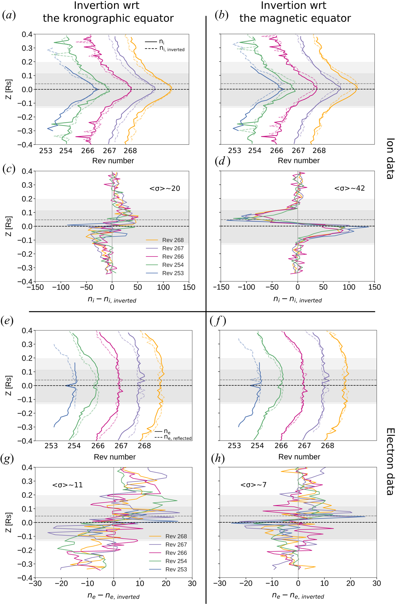
Figure 5. (a), (b) Ion density profiles ($n_{i}$ , solid lines) for all the analysed orbits compared with their mirror image ($n_{i,\, \textrm {inverted}}$
 , coloured dashed lines) with respect to the (a) kronographic equator and the (b) magnetic equator. (c), (d) Differences between the density profiles ($n_{i}$
 –$n_{i,\, \textrm {inverted}}$
 ) for (c) the equatorial plane symmetry and (d) the magnetic equator symmetry. (e)–(h) Same as (a)–(d), respectively, but for the electrons. The averaged standard deviation is given by $\langle \sigma \rangle$
 . The grey area highlights the dusty region defined as in figure 4. The grey and black dashed lines represent the magnetic and kronographic equators, respectively.
5. Discussion
Before summarising the main finding of the present work, we discuss some important points related to the estimation of $\boldsymbol {E}_{\parallel }$ near the F ring of Saturn. First, we give an estimate of the ion–dust drag force by comparing $\boldsymbol {E}_{\parallel }$
 from the individual momentum equations and highlight the importance of taking into account the presence of the charged dust. Then we address some assumptions we made in order to use the reduced form of $\boldsymbol {E}_{\parallel }$
 from (2.5).
5.1. Estimation of the ion–dust drag force
As mentioned in § 4.4, in the presence of negatively charged dust, $\boldsymbol {E}_{\parallel }$ is set up by the motion of the ions, the lighter species which are oppositely charged to the charged grains. As a consequence, $\boldsymbol {E}_{\parallel }$
 may be directly estimated using the momentum equation of the ions, given by

and should be consistent with $\boldsymbol {E}_{\parallel \textrm {tot}}$ which is derived from the combination of the force balance equations (2.5). In figure 6, we compare $\boldsymbol {E}^{(i)}_{\parallel }$
 (orange) and $\boldsymbol {E}_{\parallel \textrm {tot}}$
 (magenta) excluding the ion–dust drag term ($\boldsymbol {E}_{\Delta \boldsymbol {u}_{id}}=n_i m_i \nu _{id} (\boldsymbol {u}_d-\boldsymbol {u}_i)_{\parallel }/{q_en_i}$
 ). As one can see, in the dusty region highlighted in grey, $\boldsymbol {E}^{(i)}_{\parallel }$
 is underestimated by about two orders of magnitude. This is expected as we have neglected the dust dependance from the collisional term in expression of $\boldsymbol {E}^{(i)}_{\parallel }$
 . Therefore, the difference between $\boldsymbol {E}_{\parallel \textrm {tot}}$
 and $\boldsymbol {E}^{(i)}_{\parallel }$
 must be corrected by the ion–dust drag term that was not taken into account. Hence, in order for $\boldsymbol {E}^{(i)}_{\parallel }$
 to be of similar magnitude to $\boldsymbol {E}_{\parallel \textrm {tot}}$
 , $\boldsymbol {E}_{\Delta \boldsymbol {u}_{id}}$
 needs to be at least of the order of $5\times 10^{-6} \, \textrm {V}\, \textrm {m}^{-1}$
 . Moreover, we have added for comparison (in green) $\boldsymbol {E}^{(d)}_{\parallel }$
 obtained using the momentum equation of the dust (also neglecting the collision terms). The dominance of $\boldsymbol {E}^{(d)}_{\parallel }$
 over the other terms shows the important role of the dust in amplifying the electrostatic field. In order for $\boldsymbol {E}^{(d)}_{\parallel } \approx \boldsymbol {E}_{\parallel \textrm {tot}}$
 implies that $\boldsymbol {E}_{\Delta \boldsymbol {u}_{id}}$
 should be approximately $10^{-5} \, \textrm {V}\, \textrm {m}^{-1}$
 . The light blue curve represents $\boldsymbol {E}^{(e)}_{\parallel } \approx ({-\boldsymbol {\nabla }{_\parallel }p_e})/{q_en_e}$
 estimated using the momentum equation of the electrons. As one can note, the magnitude of $\boldsymbol {E}^{(e)}_{\parallel }$
 is about a factor of $10^2$
 less with the opposite sign. In the non-dusty scenario, one can estimate $\boldsymbol {E}_{\parallel }$
 using only the electron momentum equation; however, this is no longer valid in the presence of dust, as it leads to underestimation and the wrong direction of the ambipolar electrostatic field being obtained.

Figure 6. Ambipolar electrostatic field computed using separately the momentum equation of the ions ($\boldsymbol {E}^{(i)}_{\parallel }$ ), the electrons ($\boldsymbol {E}^{(e)}_{\parallel }$
 ) and from the general expression in (2.5) ($\boldsymbol {E}_{\parallel \textrm {tot}}$
 ). Similarly to the other figures, the grey area highlights the averaged dusty region that varied in $-0.12 \, \textrm {R}_{s} < \textrm {Z} <0.11 \, \textrm {R}_{s}$
 . The grey and black dashed lines represent the magnetic and kronographic equators, respectively.
5.2. Validity of the assumptions
Two major assumptions were made to use the reduced form of $\boldsymbol {E}_{\parallel \textrm {tot}}$ from (2.5). In the first, we neglect the presence of the magnetic mirror forces. This is justified by the near-equatorial latitudes ($< 10^\circ$
 ) at which we are focusing our analysis. As has been shown by Persoon et al. (Reference Persoon, Gurnett, Santolik, Kurth, Faden, Groene, Lewis, Coates, Wilson and Tokar2009), the role of the magnetic mirror force in Saturn's inner magnetosphere is negligible in the diffusive transport at low L-shell values ($\lesssim 5.6$
 ) and latitudes ($\lesssim 20^\circ$
 ).
).
Regarding the second assumption, we assume the sub-dominance of the neutral terms and more specifically the dust–neutral and ion–neutral drag forces in (2.4). As the measurements of neutral, dust and ion velocities along the field lines were not available during the F ring orbits, estimations of the relative velocities, $(\boldsymbol {u}_i-\boldsymbol {u}_d)_{\parallel }$ , $(\boldsymbol {u}_i-\boldsymbol {u}_n)_{\parallel }$
 and $(\boldsymbol {u}_d-\boldsymbol {u}_n)_{\parallel }$
 are not possible and neither are direct comparisons of the momentum transfer terms ($\boldsymbol {E}_{\Delta \boldsymbol {u}_{st}}=n_sm_s \nu _{st}(\boldsymbol {u}_s-\boldsymbol {u}_t)_{\parallel }/2q_en_i$
 ). Nevertheless, using the modelled ions (${\textrm {H}_{2}^+}, \, {\textrm {O}_{2}^+}$
 ) and neutral (${\textrm {H}_{2}}, \, {\textrm {O}_{2}}$
 ) densities by Tseng et al. (Reference Tseng, Johnson and Elrod2013) (figure 1b), we could estimate the collision terms $\boldsymbol {E}_{\Delta \boldsymbol {u}_{st}}/\Delta \boldsymbol {u}_{st}$
 from (2.4) and evaluate the relative values of $\Delta \boldsymbol {u}_{st}$
 . The ion–dust, ion–neutral and dust–neutral collision terms are shown in figure 7 and their expressions are respectively given by

As one can see from figure 7, ${\boldsymbol {E}_{\Delta \boldsymbol {u}_{id}}}/{\Delta \boldsymbol {u}_{id}}$ is at about two orders of magnitude larger than ${\boldsymbol {E}_{\Delta \boldsymbol {u}_{in}}}/{\Delta \boldsymbol {u}_{in}}$
 and ${\boldsymbol {E}_{\Delta \boldsymbol {u}_{dn}}}/{\Delta \boldsymbol {u}_{dn}}$
 . In other words, along the magnetic field lines, supposing that the neutrals are stationary ($\boldsymbol {u}_{n}=0$
 ), matching the dust–neutral and ion–neutral collision terms (light blue and dark blue curves,respectively) to the ion–dust term (pink curve) requires $\boldsymbol {u}_{i}-\boldsymbol {u}_{d}\sim 10^{-2} \times \boldsymbol {u}_{i}$
 at the same time as $\boldsymbol {u}_{i}-\boldsymbol {u}_{d}\sim 10^{-2} \times \boldsymbol {u}_{d}$
 , which is not possible as $\boldsymbol {u}_{d} \ll \boldsymbol {u}_{i}$
 . Therefore we can safely neglect the contribution of the neutral terms. Furthermore, as $\boldsymbol {E}_{\Delta \boldsymbol {u}_{id}}$
 should be at least $10^{-5} \, \textrm {V}\, \textrm {m}^{-1}$
 (as discussed in the previous subsection), this puts an upper limit on $\Delta \boldsymbol {u}_{id}$
 , where $\boldsymbol {u}_{i}-\boldsymbol {u}_{d} \sim 10^{6} \, \textrm {m}\,\textrm {s}^{-1} =10^{3} \, \textrm {km}\,\textrm {s}^{-1}$
 along the field lines.

Figure 7. Comparison between the ion–dust ($\boldsymbol {E}_{\Delta \boldsymbol {u}_{id}}/\Delta \boldsymbol {u}_{id}$ ), dust–neutral ($\boldsymbol {E}_{\Delta \boldsymbol {u}_{dn}}/\Delta \boldsymbol {u}_{dn}$
 ) and ion–neutral ($\boldsymbol {E}_{\Delta \boldsymbol {u}_{in}}/\Delta \boldsymbol {u}_{in}$
 ) collision terms.
6. Summary and conclusions
In summary, in this paper, we have studied the effect of the negatively charged dust on the ambipolar electrostatic field. Starting from the force balance equation and assuming diffusive equilibrium, we have derived a general expression of the magnetic field aligned ambipolar electrostatic field in the presence of negatively charged dust ($\boldsymbol {E}_{\parallel \textrm {tot}}$ ). Similarly to the dust-free plasma, the general form of $\boldsymbol {E}_{\parallel \textrm {tot}}$
 has been expressed as a function of the pressure gradient, gravitational, centrifugal, mirror and ion–neutral drag forces. In addition to these ‘classical’ terms, we have shown that $\boldsymbol {E}_{\parallel \textrm {tot}}$
 also depends on the ion–dust and dust–neutral drag forces.
Using the RPWS/LP data collected near the F ring during Cassini's ‘ring-grazing’ (Morooka et al. Reference Morooka, Wahlund, Andrews, Persoon, Ye, Kurth, Gurnett and Farrell2018), we have estimated for the first time in situ $\lVert {\boldsymbol {E}_{\parallel }}\rVert$ (approximately $10^{-5} \, \textrm {V}\, \textrm {m}^{-1}$
 ). We have shown that the nanometre-sized charged grains play an essential role in the diffusive transport of the plasma and must be taken into account: their presence amplifies the ambipolar electrostatic field by about two orders of magnitudes due to their gravitational and inertial forces. Another important result is that in the dusty region, $\boldsymbol {E}_{\parallel \textrm {tot}}$
 is asymmetric with respect to the magnetic equator (southern > northern) and reverses its direction, completely changing the dynamics in this region. Furthermore, we have discussed the role of the collision terms, in particular the ion–dust drag force, in amplifying $\boldsymbol {E}_{\parallel }$
 and give some constraints on $\boldsymbol {u}_{i}-\boldsymbol {u}_{d}$
 along the field lines. In figure 8, we summarise all these results as Cassini went through the equatorial plane close to Janus and Epimetheus faint rings, outside the main rings (see the inset).

Figure 8. Estimation of the ambipolar electrostatic field in the presence of dust (colour coded) for orbits revs 253, 254, 266, 267 and 268 as Cassini crossed the equatorial plane close to Janus and Epimetheus rings. The coordinates are defined as $X$ in the solar equatorial plane positive towards the Sun, $Z$
 northward along the spin axis of the planet and $Y$
 completing the right-handed orthogonal set. The black arrows represent the directions of $\boldsymbol {E}_{\parallel \textrm {tot}}$
 inside and outside the dusty region highlighted in grey. The inserted figure gives an overview of geometry of the highly inclined ‘ring-grazing’ orbits crossing the equatorial plane close to the F ring. The magnetic field lines were computed using the internal magnetic field model of Burton, Dougherty & Russell (Reference Burton, Dougherty and Russell2010).
Acknowledgements
Editor F. Califano thanks the referees for their advice in evaluating this article.
Declaration of interests
The authors report no conflict of interest.
Data availability statement
The Cassini RPWS/LP data are available at the University of Iowa, the Swedish Institute of Space Physics and the NASA Planetary Data System (https://pds.jpl.nasa.gov). The magnetic field data from the MAG instrument are also available on the NASA Planetary Data System archive.
Appendix A
The ion–dust collision term is given by

where $n_i$ is the total ion density measured by the LP,

is the averaged ion mass, and $\nu _{id}$ represents the Coulomb collision frequencies integrated over all the radii of the negatively charged dust that vary from $a_\textrm {min}=10^{-9} \, \textrm {m}$
 to $a_\textrm {max}=10^{-7} \, \textrm {m}$
 (expression 4.142 from Schunk & Nagy Reference Schunk and Nagy2009):

where

are the reduced mass in atomic mass units and reduced temperature in kelvins, respectively. Here $n_d=10^{-6}Ka^{-\mu }$ in $\textrm {cm}^{-3}$
 (3.1) and $m_d= \frac {4}{3}{\rm \pi} \rho a^3$
 , where $\rho =920 \, \textrm {kg}\,\textrm {m}^{-3}$
 , $K$
, $K$ (given by (3.3)) and $a$
 are in SI units.
The ion–neutral collision term is given by

where $\nu _{i\textrm {O}_2}$ and $\nu _{i\textrm {H}_2}$
 represent the elastic collision frequencies between the ions and neutrals:

where the subscript $n$ denotes the different neutral species $({\rm O}_2,H_2)$
 , $n_n$
 the corresponding neutral densities, $M_{in}$
 the reduced mass of the colliding particles and $\gamma _{{\rm H}_{2}}=0.82\times 10^{-24} \, \textrm {cm}^{3}$
 and $\gamma _{{{\rm O}_2}}=1.6 \times 10^{-24} \, \textrm {cm}^{3}$
 are the H$_2$
 and O${}_2$
 polarisabilities (table 4.1 from Schunk & Nagy Reference Schunk and Nagy2009), all expressed in cgs units.
The dust–neutral collision term is given by

where $\nu _{d\textrm {O}_2}$ and $\nu _{d\textrm {H}_2}$
 represent hard-sphere collision frequencies of the colliding particles. For them, we use expression 4.156 of Schunk & Nagy (Reference Schunk and Nagy2009):

where $k_B$ is the Boltzmann constant, and $M_{dn}$
 and $T_{dn}$
 are the reduced mass and temperature, respectively, all expressed in SI units.


 Open access