


1. Introduction
This paper investigates the role of anomalous diffusion, caused by a magnetohydrodynamic (MHD) instability, in spreading freshly accreted matter at the bottom of the massive accretion columns at the magnetic poles of ultra-luminous X-Ray (ULX) pulsars: accreting neutron stars with strong ( $B \gtrsim 10^{13}\ \textrm {G}$) magnetic fields. It should help understand the data from several X-Ray spacecraft observing ULX sources in external nearby galaxies. These objects have extremely high X-ray luminosities of approximately $10^{40}\text {--}10^{41}\ \textrm {erg}\ \textrm {s}^{-1}$, exceeding, by orders of magnitude, the Eddington luminosity $10^{38}\,(M/M_\odot)\ \textrm {erg}\ \textrm {s}^{-1}$ at which the radiation pressure force on the electrons equals the gravitational attraction on protons by an object with mass $M$. The majority of observers have traditionally believed that these sources are ‘intermediate-mass’ black holes with masses of the order of hundreds or thousands solar masses. Recently, however, the NuSTAR and Swift spacecraft detected regular pulsations with periods of the order of a second from several of such objects, implying that they are neutron stars with huge accretion rates.
X-ray binary star emission is believed to arise from mass falling from an accretion disc onto a neutron star (see Basko & Sunyaev Reference Basko and Sunyaev1976). The binary consists of a neutron star and a normal star. The normal star evolves and fills its Roche lobe with plasma that flows into the accretion disc around the neutron star. This mass is driven radially inward through the disc until it comes into contact with those outermost magnetic field lines of the neutron star. Then magnetic reconnection allows the mass to transfer to these magnetic field lines.
As the contact point of this transfer is very far from the neutron star compared with its radius, the mass is transferred to the outermost field lines, which are anchored in a very small polar region about the neutron star's magnetic axis. Then, gravity pulls the mass onto the neutron star with great velocity along the field lines and onto this polar region. We assume the radius of this region is of order of several hundred metres.
The actual details of the falling material, how it is slowed down by a radiative shock, and finally reaches the neutron star surface, are discussed by Basko & Sunyaev (Reference Basko and Sunyaev1976). In the present paper we assume that it arrives on the surface and accumulates at rest there. Our concern is what happens subsequently and how this added mass manages to merge with the ambient mass of the neutron star shell.
We assume that the neutron star has a very strong, solid, highly conducting crust below its surface. This crust forms a strong lower boundary to the outer shell of the neutron star. The plasma in this shell consists of protons and highly degenerate zero-temperature electrons. Its pressure is mainly due to the Fermi energy of the electrons. This plasma acts very much like an ordinary high-temperature plasma of high electrical conductivity. In the absence of instabilities it is strongly frozen onto the field lines of the strong  $10^{12}$– $10^{ 13}$ Gauss magnetic field of the neutron star.
The weight of the accumulating plasma quickly becomes too great to be supported by the neutron star surface and a large portion of it sinks below its surface under the influence of the gravitational field of the neutron star, and adds a large amount of pressure to the original ambient pressure of the neutron star shell. This additional pressure, localized to the polar region, pushes the shell outward from the polar axis, and as a result distorts the magnetic field.
Over time this pressure forces the incoming plasma to spread over the entire surface, greatly distorting the magnetic field of the neutron star in a way that can be observed externally. (See figures 1 and 2.)

Figure 1. There are four regions involved in the infalling plasma. In region A, the plasma is slowed down by radiation that is being emitted by the neutron star. In region B, the plasma comes to rest or is slowed down and its accumulated weight presses down on the neutron star and it submerges below the surface. In region C, the ambient plasma is pressed down and its pressure is increased. It expands radially against the plasma on closed lines. Region D, which lies on closed lines, has no new plasma until flow across the magnetic field lines occurs.
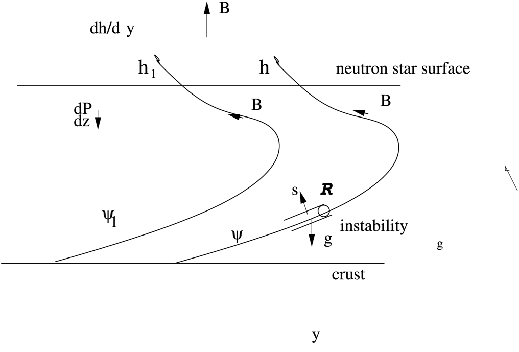
Figure 2. The region,  $\mathcal {R}$, where the instability occurs. This region is on the lower part of a line of force. The $\boldsymbol {s}$ direction perpendicular to the line of force is shown. Owing to the increase of force because of a finite gradient in $h(\psi)$, the pressure can increase in this direction and produce the instability, which always occurs on the lower part of the distorted line containing the instability.
In this paper, we explore this distorted magnetic field and the resulting redistribution of the additional plasma in the neutron star's outer shell. These depend on the flux freezing interaction between the plasma and the magnetic field. We show that when these distortions are large enough an ideal plasma instability will develop that will lead to breaking the flux-freezing constraint and allow the plasma to flow across the field lines. This cross-field flow plays an important role in the redistribution of the field lines and matter over the surface of the neutron star.
If there were no such cross-field flow, then, at any time, the amount of mass on each field line, between the crust and the surface would be equal to the amount of plasma that has fallen on it plus the ambient plasma initially on this line. For the lines on which plasma is falling, the extra mass on these lines would be equal to the amount of plasma that has flown along this line up to this time. In this paper, we refer to the inflowing plasma as simply the plasma and the ambient plasma as simply the ambient plasma.
On the other hand, in the case of no flux freezing, the mass of plasma in the outer neutron star shell will be redistributed and determined by a method we present in this paper.
Now, the distortion of the plasma and field at any time is determined by solving a certain partial differential equation called the Grad–Shafranov equation, after its relation to a similar equation in plasma physics. However, the unique solution of this equation depends on the total mass on each of the magnetic flux tubes. For this reason, it is important to show that, after the magnetic field is sufficiently stressed, a local instability develops on each field line. These instabilities cause the plasma to flow across the field lines to an extent we will determine. Thus, the equilibrium will determine the instabilities and the instabilities will determine the distribution of the plasma on the field lines, which will, in turn, determine the equilibrium.
Our theory of these instabilities is based on the similar situation that occurs in the convective region of the Sun and other stars. There, an analogous instability convects the luminosity across this region. The instability adjusts its strength to just the level necessary to provide the right convection. If the instability is too strong, too much heat flows, and if the instability is too weak, not enough heat flows. As the convective zone must carry the excess heat not carried by radiation, the instability is crucial to the structure of the Sun and stars. It turns out that the strength of this instability makes the entropy nearly adiabatic. A very similar situation holds in the neutron star's outer shell where the instability forces the magnetic type of entropy to be nearly constant, and allows the mass to flow across the magnetic field. It is this analogy which has guided our understanding of our problem.
The paper is divided into the following sections. Section 2 describes the condition for static equilibrium.
Section 3 describes the instability and the conditions for the equilibrium to be unstable to it on any line.
In § 4, we describe the nonlinear properties of the instability and describe the cascade of fluctuations of the magnetic field strength and plasma density which it produces. We present a simple physical picture as to how, when the eddies reach the resistive scale, the magnetic strength and plasma density fluctuations cause mass to cross the magnetic field lines.
In § 5, the analytic details of the evolution of the cascade is presented and the rate of cross-field flow is calculated. An example is given to show how close to marginality all the instabilities need to be for a steady state in an actual case.
Section 6 shows that the quasi-static equilibrium is a sequence of marginally stable states and how they are controlled by the plasma inflow onto the neutron star.
Section 7 describes other research on this problem.
Section 8 summarizes the results and draws the conclusion promised in the introduction as to the method of determining the distribution of the mass per flux and the distortion of the outer shell.
There are several appendices that supplement the calculations in the text. Appendix D presents a very approximate attempt to predict the long-time behaviour of the neutron star's shape distorted by the flow.
2. The equilibrium
The rate of the infalling plasma on the neutron star is slow enough that the equilibrium, under the combined pressure gradient, gravitational and magnetic forces, is essentially static. (We neglect the centrifugal force owing to the star's rotation.) At first, we consider the equilibrium only in the region near the north pole. The symmetric solution holds near the south pole.
This equilibrium is described by the so-called Grad–Shafranov equation.
Let the incoming matter and the neutron star's magnetic field be axisymmetric about its axis and have no toroidal component. At first, we restrict ourselves to times before the infalling matter has spread over a large region of the neutron star's surface, so that we are able to treat the ambient surface as planar. We employ cylindrical coordinates,  $r, \theta , z$, and take the ambient outward magnetic field that existed before the infall of any matter, as uniform, of constant strength $B_0$ and parallel to the axis of symmetry. The $\boldsymbol {z}$ coordinate increases radially inward so that $z$ gives the depth below the ambient surface. Therefore, $\boldsymbol {B}_0$ is in the negative $\hat {z}$ direction (i.e. vertically upward). We assume that the gravitational field $\boldsymbol {g}$ is constant, of magnitude $g$ and is in the positive (downward) $z$ direction. The surface $z=0$ is the ambient neutron star surface, that exists before any mass has fallen. All quantities are in cgs units.
The components of the magnetic field can be expressed in terms of its flux function  $\psi$ as
 \begin{equation} B_r= -\frac{1}{r} \frac{\partial \psi }{\partial z} ; \quad B_z= \frac{1}{r} \frac{\partial \psi }{\partial r} . \end{equation}
Here  $\psi=$ constant is a flux surface (as $\boldsymbol {B} \boldsymbol {\cdot } \boldsymbol {\nabla } \psi =0$). The function $\psi (r,z)$ is, thus, equal to $1/2 {\rm \pi}$ times the magnetic flux enclosed by the magnetic surface through $r$ and $z$.
$z$.
The current density,  $\boldsymbol {j}$, which is in the $\theta$ direction, is
 \begin{align} 4 {\rm \pi} j_\theta &= \frac{ \partial B_r}{\partial z}- \frac{ \partial B_z}{\partial r} \nonumber\\ &= -\frac{\varDelta^{*} \psi }{r}, \end{align}
where
 \begin{equation} \varDelta^{*} \equiv \left(\frac{\partial^2 }{\partial r^2} -\frac{1}{r} \frac{\partial }{\partial r} + \frac{\partial^2 }{\partial z^2} \right). \end{equation}
Now, for a magnetostatic equilibrium,
 \begin{equation} \boldsymbol{j} \times \boldsymbol{B} = \boldsymbol{\nabla} p -\rho \boldsymbol{g} . \end{equation}
The radial component of this equation is
 \begin{equation} - \frac{1}{4 {\rm \pi} r^2} (\varDelta^*\psi) \frac{\partial \psi }{\partial r}= \left( \frac{\partial p }{\partial r} \right)_z , \end{equation}
where  $p$ is at first taken as a function of $z$ and $r$.
$r$.
The neutron star pressure is mainly due to cold degenerate electrons for which  $p= p(\rho)$. Non-relativistically, in cgs units $p =1.0 \times 10^{ 13} \rho ^{5/3}$, and ultrarelativistically, $p= 1.5 \times 10^{ 15} \rho ^{4/3}$. In general, we write $p=K \rho ^{\gamma _{A}}$ where $\gamma _{A}$ is the adiabatic index, 5/3 in the non-relativistic limit and 4/3 in the ultrarelativistic limit.
The component of (2.4) parallel to the magnetic field is
 \begin{equation} \frac{\textrm{d} p}{\textrm{d} \rho } \left( \frac{\partial \rho }{\partial z}\right)_{\psi} = \rho g , \end{equation}
where the subscript  $\psi$ indicates the $z$ variation at constant $\psi$, i.e. taken along a fixed line $\psi$. Its non-relativistic solution is
 \begin{equation} \rho(z, \psi) = 22.6 (z+\textrm{const})^{3/2} . \end{equation}
We have taken  $g= 2 \times 10^{14}\ \textrm {cm}\ \textrm {s}^{-2}$. The integration constant is to be determined on each line by the boundary condition at the surface. It should be zero when $z = -h(\psi)$ at the top of the accumulated plasma, which rises a height $h(\psi)$ above the ambient surface. Thus,
 \begin{equation} \rho(\psi,z) =22.6 [z+h(\psi)]^{3/2}\ \textrm{g}\ \textrm{cm}^{-3} , \end{equation}
and
 \begin{equation} p(z,h)=1.83 \times 10^{ 15}(z+h)^{5/2}\ \textrm{ergs}\ \textrm{cm}^{-3} . \end{equation}
Cancelling the factor  $(\partial \psi /\partial r)$, the non-relativistic Grad–Shafranov becomes
 \begin{equation} - \frac{\varDelta^* \psi }{4 {\rm \pi} r^2} = 4.58 \times 10^{ 15} [z+h(\psi)]^{3/2} \frac{\textrm{d} h}{\textrm{d} \psi } . \end{equation}
 In the relativistic region, the pressure is more complex because when the electron Fermi energy is greater than 2 MeV, the electrons combine with protons to make neutrons. The resulting equation of state for relativistic degenerate electrons in neutron stars is quite complicated and is discussed in chapter 3 of Shapiro & Teukolsky (Reference Shapiro and Teukolsky1983). We do not get into the details and simply use  $P_{\textrm {am}} (z)$ for the ambient non-relativistic and relativistic pressures.
For the general case, let  $P_{\textrm {am}}(z)$ and $\rho _{\textrm {am}}(z)$ be the hydrostatic solution for the ambient pressure and density. Then, because the hydrostatic equation (2.6) does not involve $z$,
$z$,  $P_{\textrm {am}}[z+h(\psi)]$ and $\rho _{\textrm {am}}[z+h (\psi)]$ are also solutions along $B$ with the pressure and density still related by the same equation of state. This latter solution is the hydrostatic solution of a column of plasma lifted by a height $h(\psi)$ along the line of force $\psi$. Thus, we have
 \begin{equation} p(z, \psi) = P_{\textrm{am}}[z+h(\psi)] \end{equation}
is valid for a plasma that rises a height  $h(\psi)$ above the neutron star surface. The general Grad–Shafranov equation (2.5) is then
 \begin{equation} -\frac{1}{4 {\rm \pi} r^2} \varDelta^* \psi = \frac{\partial P_{\textrm{am}}}{\partial z} \left[ z+h(\psi)\right] \frac{\textrm{d} h}{\textrm{d} \psi }. \end{equation}
 However, the equations for the pressure and density are not valid within a distance  $h(\psi)$ of the crust and the pressure and density have been extended by a Taylor expansion of $p$ and $\rho$. To lowest order, in this expansion the density is a constant equal to the ambient density at the crust, $\rho _{\textrm {crust}}$. In addition, the conductivity of the crust is so large that the magnetic lines of force are frozen in it and do not move during the distortion. The primeval mass per flux in the extension is equal to this density times the volume which equals the height times the cross-sectional area of the flux tube; therefore, $m(\psi)$, the extra mass of the fallen matter per $\textrm {d} \psi$, is
 \begin{equation} m(\psi) = \frac{h(\psi) \rho_{\textrm{crust}}}{B_0} . \end{equation}
 Here  $2 {\rm \pi} m(\psi)$ is the mass per flux. We see that the function $h(\psi)$ has three different interpretations. It gives the height of the plasma above the neutron star surface, the extra mass per unit flux and the right-hand side of the Grad–Shafranov equation. As it gives the distribution of mass, it should lead to a unique static solution as can be seen by an energy argument. The equilibrium state with a given distribution of mass on flux tubes is the lowest energy state with this constraint.
Thus, the determination of  $h(\psi)$ is a fundamental problem. Its determination is related to our main question of whether there are any cross-field flows. The answer to this question is related to the existence of an instability on each line which has the capacity to drive these flows. A quasi-steady state depends on there being some cross-field flows at every line of force and, therefore, on there being an instability driving turbulent transport.
3. The instability
In general, every line of force in the static equilibrium may be subject to our instability. We present a simplified derivation of this instability here. A more rigorous derivation, based on the MHD energy principle, is given in appendix A.
In figure 2, consider a particular small region on the lower part of a line of force, and let us visualize it in local coordinates (see figure 3).
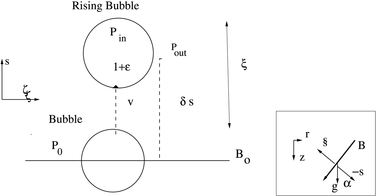
Figure 3. The diagram of the elementary physics of the buoyant instability. The orientation of the instability is indicated by the direction  $\boldsymbol {s}$ in which the buoyancy occurs. This direction is at an angle to $\boldsymbol {g}$. The coordinates of the instability are indicated, and $\alpha$ is the angle between $-\boldsymbol {s}$ and $\boldsymbol {g}$.
The instability occupies a cylindrical region  $\mathcal {R}$ on the lower part of a line of force as shown in figure 2. It extends a distance $\ell$ along this line of force. We describe the instability in the localized Cartesian coordinates, $s,y,\zeta$, where $\zeta$ is taken along the line on which the plasma is unstable, $y$ is in the $\theta$ direction and $s$ is perpendicular to $\zeta$ in the $r z$ plane and increases towards the axis. Here $g_s = g \cos \alpha$ is the component of $\boldsymbol {g}$ in the negative $\boldsymbol {s}$ direction where $\alpha$ is the angle between $-\boldsymbol {s}$ and $\boldsymbol {z}$.
We assume that the region  $\mathcal {R}$ extends a sufficient distance along the magnetic line that locally the motions are two-dimensional and independent of $\zeta$. The lines that are straight and rigid will roll over each other. At first, we ignore any tension forces associated with the ends of the region.
In these coordinates, the initial ambient pressure,  $p$, decreases along $\boldsymbol {s}$ as $\psi$ decreases, but after being upshifted by $h(\psi)$ the total distorted pressure may actually increase. The magnetic field strength $B$ decreases along $\boldsymbol {s}$ because the magnetic field is pushed outward by the added infalling mass.
As in the solar case, described in Schwarzschild (Reference Schwarzschild1958), consider a two-dimensional (cylindrical) bubble rising a small distance  $\delta s$ away from the original line. Let the bubble expand its volume slightly by a factor $1 + \epsilon$. Inside the bubble, the density will change by the factor $(1 -\epsilon)$ and the plasma and the magnetic pressures will change by factors of $(1 -\epsilon) ^{\gamma _A}$ and $(1 -\epsilon)^{2}$.
The total pressure inside the bubble will be
 \begin{align} P_{\textrm{in}} =\left( p +\frac{B^2}{8 {\rm \pi} }\right) &= p_0 (1 -\epsilon)^{\gamma_A} +\frac{B_0^2}{8 {\rm \pi} } (1-\epsilon)^2 \nonumber\\ &= p_0 + \frac{B_0^2}{8 {\rm \pi} } - \left( \gamma_A p_0 + 2 \frac{B_0^2}{8 {\rm \pi} }\right) \epsilon , \end{align}
where the zero index refers to the bubble's initial pressure and magnetic field strength. The total pressure outside the bubble in the undisturbed plasma and magnetic field is
 \begin{equation} P_{\textrm{out}} =\left( p_0 +\frac{B_0^2}{8 {\rm \pi} }\right) + \left( p'_0 + \frac{B_0 B_0'}{4 {\rm \pi}} \right) \delta s , \end{equation}
where throughout the rest of this paper (except in one case), a prime will always denote an  $s$ derivative.
If the bubble rises slowly enough, the total pressure inside the bubble must equal that outside it. Thus,  $P_{\textrm {in}}= P_{\textrm {out}}$ and, hence,
 \begin{equation} \epsilon = \frac{-P_0'}{\varGamma P_0} \delta s . \end{equation}
where  $\varGamma P_0 = \gamma _A p_0 +2 B_0^2/8 {\rm \pi}$. Thus, $\varGamma$ is the effective adiabatic index for the total pressure $P_0 = p_0+ B_0^2/8 {\rm \pi}$.
The gravitational (buoyancy) force per unit volume on the bubble in the  $\boldsymbol {s}$ direction, $F_s$, is
 \begin{equation} F_s =-g_s( \rho_{\textrm{in}} -\rho_{\textrm{out}}) = -g_s [ -\epsilon \rho_0 -(\delta s) \rho_0')] = - g_s \rho \left( \frac{ P_0'}{\varGamma P_0 } -\frac{\rho'_0}{\rho_0} \right) \delta s . \end{equation}
 Now, from our equation of state  $p'/p = \gamma _A \rho ' /\rho$, so expanding the expression in the parentheses and dropping the zero subscripts, we obtain
 \begin{align} \frac{P'}{\varGamma P}-\frac{\rho' }{\rho } &=\frac{ P'}{\varGamma P }-\frac{p' }{\gamma_A p } \nonumber\\ &= \frac{1}{4{\rm \pi} \varGamma P \gamma_A p}[\gamma_A p ( B B' + 4{\rm \pi} p') - p' ( B^2+ 4 {\rm \pi} \gamma_{A} p)] \nonumber\\ &= \frac{1}{4 {\rm \pi} \varGamma P \gamma_A p} ( \gamma_A p B' B - p' B^2) \nonumber\\ &= \frac{B^2}{4 {\rm \pi} \varGamma P \gamma_A } \left( \frac{\gamma_A B' }{B } - \frac{ p' }{p } \right)= \frac{1}{\gamma_A (1+\gamma_A \beta/2)} \left( \frac{ \gamma_{A} B'}{B}-\frac{p'}{ p}\right) . \end{align}
 As a result the force in the  $\boldsymbol {s}$ direction is
 \begin{equation} F_s =\frac{g_s \rho}{\gamma_A} \frac{\varDelta }{ (1 + \gamma_A \beta/2) } \delta s =g_s \rho \frac{\varDelta }{C} \delta s , \end{equation}
where
 \begin{align} \varDelta &= \frac{p'}{p} -\gamma_A \frac{B'}{B} \nonumber\\ =& \frac{\textrm{d}}{\textrm{d}s} \ln{ \left( \frac{p}{B^{\gamma_A}}\right) } , \end{align}
and
 \begin{equation} C=\gamma_{A} (1+\gamma_{A} \beta /2). \end{equation}
As usual,  $\beta \equiv 8 {\rm \pi} p/B^2$. In the ambient medium $\beta = 4.6 \times 10^{ -8} z^{2.5}$ for $B=10^{ 12} \ \textrm {G}$. The factor $C$ depends on $\beta$. When $\beta$ is small, $C$ is $\approx \gamma _{A}$, and when $\beta$ is large, $C$ is of the order of $\gamma _{A}^2 \beta /2$. We treat $C$ as of order one in our estimates.
The product  $g_s \varDelta$ is the critical stability quantity. Assuming $g_s >0$, as is the case on the lower part of a line of force (see figure 2), $\varDelta$ must be positive for instability. If $g_s < 0$, as is the case on the upper part of the line, then $\varDelta <0$ is the condition. However, on this upper part of the line $\varDelta$ is almost always positive and there is no instability.
This instability was discovered by Newcomb (Reference Newcomb1961), and he derived its force in the form given in the parentheses of (3.4). We have reduced it to the form given in (3.6), which is more convenient for our purposes.
It is useful to express  $\varDelta$ approximately in terms of the density gradient. In the local approximation, we assume $p' + B B'/4 {\rm \pi} \approx 0$ because the gravitational and curvature forces are small compared with the gradient forces in a thin region. In addition, $p'/p =\gamma _{A} \rho '/\rho$ for degenerate electrons.
Then it is easy to show that
 \begin{equation} \varDelta \approx C \frac{\rho'}{\rho} , \end{equation}
thus we have an instability if  $\rho '$ (or $p'$) is greater than zero on the lower parts of the lines.
Further, using (2.11), we obtain
 \begin{align} p' &= \frac{\textrm{d} P_{\textrm{am}}[z + h] }{\textrm{d} s} = \frac{\textrm{d} P_{\textrm{am}}}{\textrm{d} z} \left( \frac{\textrm{d} z}{\textrm{d} s} +\frac{\textrm{d} h}{\textrm{d} s} \right) \nonumber\\ &= \frac{\textrm{d} P_{\textrm{am}}}{\textrm{d} z}(-\cos \alpha +\textrm{d}h/\textrm{d}s) , \end{align}
where  $\alpha$ is the angle between the $- \boldsymbol {s}$ and $\boldsymbol {z}$. Therefore, (because $\textrm {d} P_{\textrm {am}}/\textrm {d} z$ is positive), on the lower part of the line where $g_s>0$ the plasma is unstable if and only if
 \begin{equation} \frac{\textrm{d} h}{\textrm{d}s} > \cos \alpha . \end{equation}
 Thus, if  $h$ changes fast enough in the $s$ direction, then one has instability. In other words, if too much mass accumulates inside the flux surface of the line, $\textrm {d}h/\textrm {d}s$ will be large enough to produce the instability as was hinted at in the introduction.
In our derivation of the stability condition, we have neglected the fact that our cylindrical bubble has ends and we have assumed that the magnetic field is only locally perturbed along a length  $\ell$ and is unperturbed outside. However, there is a tension force ${\rm \pi} B_0^2(\delta s/\ell ^2)$ per unit volume. Thus, $\varDelta$ must be greater than zero for instability. An estimate shows that the critical value of $\varDelta$ for instability is
 \begin{equation} \varDelta_{\textrm{crit}} =\frac{{\rm \pi}^2 v_A^2 C}{g_s \ell^2 }. \end{equation}
 Thus, the critical condition for instability is  $\varDelta '= \varDelta -\varDelta _{\textrm {crit}} >0$. (This prime does not refer to a derivative.) When necessary, we can take care of the tension forces by replacing $\varDelta$ by $\varDelta '$. It turns out that in our applications $\varDelta '$ is very close to $\varDelta$ so, where appropriate in our subsequent discussions, we can replace $\varDelta '$ by $\varDelta$.
The quantity  $\varDelta$ is a function of $s$ through the $s$ dependence of $p'/p$ and $B'/B$, so that the force $F_s$ will be positive over a limited region $- \xi < s < \xi$, where $\xi$ is a mixing length, whose magnitude we estimate in § 5. The force $F_s$ is the gradient of a local potential. If, for simplicity, we take the potential as parabolic, its depth is
 \begin{equation} \phi = \rho g_s \frac{\varDelta }{2 C} \xi^2 . \end{equation}
As an approximation to the nonlinear orbit of the unstable fluid element, we can take its corresponding velocity as a harmonic motion with amplitude
 \begin{equation} v_0 = \xi \sqrt{\frac{g_s \varDelta }{C}}\ \textrm{cm}\ \textrm{s}^{-1}. \end{equation}
 It is useful to have some idea as to the magnitude of these quantities. With  $g = 2 \times 10^{14} \ \textrm {cm}\ \textrm {s}^{-2}$ and the mixing length $\xi =10^{3}\ \textrm {cm}$, the velocity is $v_0 =1.4 \times 10^{10} \sqrt { \varDelta /C}\ \textrm {cm}\ \textrm {s}^{-1}$. We expect $\varDelta$ to be at most of order $10^{-4}\ \textrm {cm}^{-1}$ because it is the difference of the gradient of two equilibrium quantities and we take their scale heights as of order $10^{4}\ \textrm {cm}$. Thus, (in this case) $v_0$ should be at most $1.4 \times 10^{8}\ \textrm {cm}\ \textrm {s}^{-1}$. The nonlinear growth rate $\gamma _{\textrm {nl}} \equiv k_0 v_0/2$, where $k_0 =2 {\rm \pi} / \xi$, is from (3.14)
 \begin{equation} \gamma_{\textrm{nl}} =\frac{k_0 v_o}{2} ={\rm \pi} \sqrt{\frac{g_s \varDelta }{C}}, \end{equation}
thus  $\gamma _{\textrm {nl}} =4.4 \times 10^{ 7} \sqrt {\varDelta /C}\ \textrm {s}^{-1}$, or at most $4.4 \times 10^{ 5}\ \textrm {s}^{-1}$.
When the instability becomes nonlinear, we expect there to be many such independent unstable modes in the unstable  $k$ region. Treating the modes as independent, and adding all of these modes, we can treat the resulting velocity field statistically.
Expand  $\boldsymbol {v}$ in a two-dimensional Fourier series in $\boldsymbol {k}$ and a Fourier integral over $\omega$,
 \begin{equation} \boldsymbol{v} = \varSigma_{\boldsymbol{k}} \int\ \textrm{d} \omega \boldsymbol{v}_{\boldsymbol{k}\omega } \exp({\textrm{i} \boldsymbol{k} \boldsymbol{\cdot} \boldsymbol{r} - \textrm{i}\omega t}). \end{equation}
We assume that  $\boldsymbol {v}$ is perpendicular to $\boldsymbol {B}_0$ and independent of $\zeta$, the coordinate along $\boldsymbol {B}_0$.
Then, we use the random phase approximation to write
 \begin{equation} \langle \boldsymbol{v}_{\boldsymbol{k'}\omega'}^{*} \boldsymbol{v}_{\boldsymbol{k}\omega }\rangle = J(k,\omega) \delta_{\boldsymbol{k'} \boldsymbol{k}} \delta (\omega' - \omega) (\boldsymbol{I} - \hat{\boldsymbol{k}} \hat{\boldsymbol{k} } ) . \end{equation}
Here,  $J(k, \omega)$ is the turbulent velocity spectrum that we assume axisymmetric about the magnetic field direction.
Although one expects nonlinear effects to spread the unstable velocities over many different wave length scales, we make the simplifying assumption that all the velocity modes remain on the scale of the inverse mixing length,  $k_o= 2 {\rm \pi} / \xi = 6.7 \times 10^{-3}\ \textrm {cm}^{-1}$. However, the frequency of the velocity modes is not monotonic.
4. The cascade of the fluctuations of the magnetic field strength
Using these facts about the instability, we are now in a position to discuss the nonlinear cascade developed by the instability, when it saturates and how it can move plasma across the very strong neutron star magnetic field lines.
We assume that the turbulent velocities are localized to the cylindrical region  $\mathcal {R}$ of radius $\xi$ and length $\ell$ along a given field line. Outside this region in the longitudinal direction along $\boldsymbol {B}_0$, or in the radial direction across $\boldsymbol {B}_0$, the plasma will be stable and there will be no turbulent velocity (see figure 2). Owing to the great strength of the magnetic field, its lines of force will be straight and rigid during the perturbations. However, as they are displaced, the magnetic strength at a fixed point varies.
Inside  $\mathcal {R}$, the turbulent velocities move the straight magnetic field lines around, mixing them up. These lines will remain tied to the static outside lines so this line tying will lead to tension that will try to keep the lines in $\mathcal {R}$ from moving. As long as the instability persists owing to a non-zero (positive) $\varDelta ^{*}$, the unstable forces will be able to overcome the tension forces and mixing will continue.
Even though we have assumed that the transverse turbulent velocities remain on the mixing length scale  $k_0$, these velocities will have a shear that can generate magnetic and density perturbations at much smaller scales. As long as the plasma is ideal, these perturbations will extend down to the smallest conceivable scales. However, at sufficiently small scales, resistive effects become important and truncate the magnetic and density spectra. On these scales, the plasma will no longer be ideally tied to individual lines, and resistivity can lead to transfer of mass between different lines.
The combination of these two effects, namely the propagation of the perturbations down to resistive scales and the transfer of mass to different lines on these scales, leads to systematic motions of the plasma across the lines. With time, these motions flatten the density gradient, which was driving the instability and it will terminate. Finally, the lines in  $\mathcal {R}$ will have returned to their original position under the influence of the tension force tying the lines to the external region, but the plasma will not have returned to its original position. On the contrary, some of the plasma will have moved downstream in the negative $s$ direction. In this way, flux freezing will be broken, there will be a bulk motion of the plasma across the lines and the accumulated infalling mass will be able to spread over the neutron star without completely dragging the field lines with it.
The rest of the paper is devoted to deriving the rate at which this all happens.
Before proceeding to an analytical treatment of the evolution of the fluctuation spectrum let us pause and understand in a general way what is going on. We do this by making use of a simple model (see figures 4 and 5).

Figure 4. Side view of the model. The region  $\mathcal {R}$ is indicated in which the rods exist. Their size is the resistive size. Two particular rods $\phi _1$ and $\phi _2$ are shown. They are being mixed up by the eddies produced by the turbulent velocity shear.

Figure 5. End-on view of the model.  $(a)$ The two rods $\phi _1$ and $\phi _2$ with different densities are initially some distance apart. $(b)$ After some time they are brought close together and resistive effects will cause the plasma to flow between the rods and equalize their densities. A repetition of these collisions will equalize the densities of all the rods. $(c)$ Plot of how the density would vanish along a cross cut of the region.
Imagine the magnetic field strength and density having fluctuations at only a single scale, say the scale  $k_{\eta }$. Ignoring the region along $\boldsymbol {B}_0$ outside of $\mathcal {R}$, which is stable, let us replace the magnetic field by a large collection of rigid rods oriented in the $\boldsymbol {B}_0$ direction with radii of the order of this scale (see figure 4). Let each of the rods, which we label by $\phi$, internally contain a uniform plasma and magnetic field, whose density and strength can be different for different rods. Let the rods be moved around randomly by the shear of large-scale turbulent velocities, which are perpendicular to the rods and uniform in $\ell$ (i.e. rolls).
As the rods move, let them remain rigid. Initially, let the different plasmas in the rods vary in space in a way consistent with the unstable equilibrium. Let the mass in each individual rod remain constant as the rods move.
In figure 5, we display an end view of the rods. At first, neighbouring rods will have nearly the same densities. After the rods are mixed up by transverse motions, two rods  $\phi _1$ and $\phi _2$ in figure 5(a) with quite different densities and field strengths may come close together as in figure 5(b). When this happens a surface current $\boldsymbol {j}$ develops between the two rods. From Ohm's law in the frame of motion $\boldsymbol {v} \times \boldsymbol {B} = \eta \boldsymbol {j}$, this current will give rise to diffusional velocity of plasma between the two rods. It is easy to see that if the rods both have the same total pressure $p + B^2/8 {\rm \pi}$ the diffusion is from the high-density to the low-density rods and this equalizes their two densities.
If the mixing continues long enough, all the neighbouring pairs in the same neighbourhood will approach each other and all the densities in the entire cylindrical region will equalize. As a consequence the unstable density gradient  $\rho ' = \rho \varDelta /C$ driving the instability will be reduced to zero, and the turbulent velocity driving the mixing will cease.
However, when one compares the original density, which had a finite gradient, with the final density, which has a stable gradient, we see that the plasma will have been shifted relative to the magnetic field lines, see figure 6. Thus, when the turbulent cascade reaches the resistive scale, it is truncated by the resistive effects described previously, which flatten the magnetic and density gradients and damp the instability.

Figure 6. An explanation of why some mass can cross magnetic field lines. A plot of the density before and after the instability. Before the instability develops, there is an unstable gradient of the density in the  $s$ direction, which produces a cascade (here, $s$ increases to the left). After the cascade saturates, the density gradient vanishes and the mass distribution becomes different, so that there is less mass upstream (positive $s$) and more mass downstream, violating flux freezing. The density before is indicated by lines slanting to the left and after lines slanted to the right.
We see that the cascade proceeds in two stages. In the first stage, the fluctuations of  $B$ and $\rho$ cascade down the scales to a size where resistive effects come into play. We show in the next section that this happens at a rate of order $\gamma _{\textrm {nl}}/16$, see also appendix B. In the second stage, the resistive effects will flatten the density spectrum at the resistive diffusion rate $k^2 \eta$ (see appendix C). At large scales, this diffusion rate is small compared with the cascading rate, but at a certain scale $k_{\textrm {eq}}$, it will balance the rate of flow of the first stage so as the fluctuations propagate down the cascade they will be damped by the second stage effects. This scale will be roughly equal to $k_{\eta }$ where
 \begin{equation} k_{\eta}^2 \eta = \gamma_{\textrm{nl}} . \end{equation}
At still shorter wave lengths there will be no fluctuations.
We will separate these two stages. In the first stage, treated in the next section, we will derive the evolution of the magnetic strength fluctuations as though there were no resistivity. In the second stage treated in appendix C we will derive the resistive damping for  $k \approx k_{\eta }$. Then we will match the two rates to find the scale $k_{\textrm {eq}}$ where the two rates balance. The first scale is characterized by a the time $t_{\gamma , D}$ for the cascade to reach $k_{\eta }$. and the second is characterized by the resistive time, $t_{\eta ,D}$, at $k_{\eta }$. Once the two times have been found a simple iteration leads us to $k_{\textrm {eq}}$. We will find that the two times do not balance. We will then alter $k$ to get balance, and find $k_{\textrm {eq}} = 4.5 k_{\eta }$.
The mathematical details of the first stage are given in the next section and the second stage in appendix C.
The total life of the instability from its initial time to the time when it is terminated is
 \begin{equation} t_D = t_{D \gamma } + t_{D \eta} \end{equation}
with the times first evaluated for  $k = k_{\eta }$ and then for $k_{\textrm {eq}}$.
4.1. The rate of mass flow across magnetic lines
We can express the flow rate in terms of the instability lifetime  $t_D$ as follows. After the instability is terminated, the initial density gradient has been reduced by
 \begin{equation} \delta \rho' = \rho_0 \varDelta / C , \end{equation}
where  $\rho '$ is the initial gradient and the final gradient is zero, see (3.9).
After the cascade has terminated an amount of mass per unit area
 \begin{equation} \delta M = \frac{\xi^2 \delta \rho'}{ 2} = \frac{\varDelta}{C} \frac{\rho_0 \xi^2}{2 } \ \textrm{g}\ \textrm{cm}^2\ \textrm{s}^{-1} \end{equation}
will have been transferred across the plane  $s =0$ by the cascade, see figure 6. Dividing this mass by $t_D$, the life of the instability, we obtain the average rate of the local mass flow across the magnetic lines during the life of this instability
 \begin{equation} \frac{ \delta M}{t_D} = \frac{\rho_0 \xi^2}{2 t_D} \frac{\varDelta}{C} . \end{equation}
 So far, we have concentrated on the flow of local mass in region  $\mathcal {R}$ crossing the magnetic field the field line. However, in a steady state all the mass in the entire flux tube must cross the field (see figure 7). However, the flow along the field line is easy so that as the local mass is removed from the unstable region, a pressure gradient will exist along the line which will pull the plasma to the unstable region. This happens fast enough that one sees a continual flow of the total mass across the field. If $\epsilon$ is the fraction of the line's length in the unstable region, then the amount of mass needed to be transferred will be larger by a factor approximately $1/\epsilon$. However, the time for complete transfer will be longer by the same factor. Thus, (4.5) still gives the mean flow during the life of the instability.

Figure 7. The correction for the flow along field lines. The mass along the entire fluid slows along the tube until it reaches the instability and crosses the line at that point, increasing the length of the flow time, but increasing the amount of mass during the longer time.
Assuming that the instabilities are continually excited with the same  $\varDelta$, this expression yields the relation between the mean cross-flow rate and $\varDelta$, once the life of the instability $t_D$ is known. Our goal is thus reduced to evaluating $t_D$.
5. The evolution of the cascade
In this section, we derive the ideal equation for the time-dependent spectrum of the intensity of the magnetic fluctuations at a general point and time of the quasi-static equilibrium.
Let the field strength be
 \begin{equation} B=B_0 + b(\boldsymbol{x} ,t), \end{equation}
where  $B_0$ is the unperturbed quasi-static magnetic field. The initial unstable gradient of the magnetic field strength is included in $b$.
$b$.
We assume  $\boldsymbol {\nabla } \boldsymbol {\cdot } \boldsymbol {v} =0$ because the magnetic field is so strong. Then the magnetic field strength satisfies the scalar equation
 \begin{equation} \frac{\partial b}{\partial t} = -\boldsymbol{\nabla} \boldsymbol{\cdot} (\boldsymbol{v} b) . \end{equation}
 If we perform a Fourier analysis of  $b$,
$b$,
 \begin{equation} b= \varSigma_{\boldsymbol{k}} b_{\boldsymbol{k}}(t) \exp({\textrm{i} \boldsymbol{k} \boldsymbol{\cdot} \boldsymbol{x} }), \end{equation}
then this equation can be written as
 \begin{equation} \frac{\partial b_{\boldsymbol{k}} }{\partial t} = - \textrm{i} \boldsymbol{k} \boldsymbol{\cdot} \int \varSigma_{\boldsymbol{k''}} \left( \boldsymbol{v}_{\boldsymbol{k''}} b_{\boldsymbol{k'} } \right) \,\textrm{d} \omega , \end{equation}
where we use the notation
 \begin{equation} \boldsymbol{k} = \boldsymbol{k'} + \boldsymbol{k^{\prime\prime}} . \end{equation}
This equation can be interpreted as a  $\boldsymbol {k}$ magnetic mode being changed by the interaction of a $\boldsymbol {k''}$ velocity mode with another $\boldsymbol {k'}$ magnetic mode. The integration over $\textrm {d}\omega$ allows for the time dependence of the turbulent velocity.
This equation is of the same type as the dynamo equation treated by Kulsrud & Anderson (Reference Kulsrud and Anderson1992), which itself is equivalent to the direct-interaction formalism of Kraichnan & Nagarajan (Reference Kraichnan and Nagarajan1967). It can be solved in a similar way with two changes. Here the perturbed magnetic field strength  $b$ is the passive scalar. Further, the velocities are perpendicular to the unperturbed $\boldsymbol {B}_0$ and independent of the position along the unperturbed field line. The details of the solution, with the appropriate modifications, are given in appendix B.
We have used discrete Fourier modes for the analysis because they make the direct interaction between the turbulent velocity and the magnetic field clearer. The Fourier series are most easily interpreted in terms of continuous functions, so with box normalization, we replace an axisymmetric sum of the square of the Fourier modes by
 \begin{equation} \varSigma_k |b_{\boldsymbol{k}}|^2 = \int M(k)\,\textrm{d}k. \end{equation}
Thus,  $M(k)$, is the spectrum of the intensity of the perturbations in the magnetic field strength. In the box normalization formalism $M(k)$ is defined by
 \begin{equation} M(k) = \left(\frac{L}{2 {\rm \pi} } \right)^2 \int |b_{\boldsymbol{k}}|^2 k\,\textrm{d} \hat{\boldsymbol{k}}, \end{equation}
where  $L^2$ is the two-dimensional volume of our box, $k$ is a scalar, $\boldsymbol {\hat {k}}$ is a unit vector and the integral is over a cylindrical surface of radius $k$.
$k$.
As shown in appendix B, for  $k \gg k_0$ the time evolution of $M(k)$ is given by the differential equation
 \begin{equation} \frac{\partial M}{\partial t} = \frac{\gamma }{16} \left( k^2 \frac{\partial^2 M}{\partial k^2} +k \frac{\partial M}{\partial k} - M \right), \end{equation}
where from (B 28)
 \begin{equation} \gamma = \left( \frac{L}{2 {\rm \pi} } \right)^2 \int k''^2 J(k'',0) d \boldsymbol{k}'' . \end{equation}
 (This ignores the fact that (5.8) for  $\partial M(k)/\partial t$ is actually the large $k$ limit of an integral equation. Assuming the differential equation is valid down to $k_0$ does make a small error. However, because the range in $k$ is very large this is probably not serious.)
We have assumed that the velocity spectrum is concentrated at  $k_0$. Then from this equation for $\gamma$ and (3.17)
 \begin{equation} v_0^2 = 2 \left(\frac{L}{2 {\rm \pi} } \right)^2 \int J((k^{\prime\prime},\omega)\,\textrm{d}^2 \boldsymbol{k}^{\prime\prime}\,\textrm{d} \omega , \end{equation}
it follows that
 \begin{equation} \frac{\gamma}{ v_0^2} = \frac{k_0^2}{2} \frac{ J(k,0)}{\int J(k,\omega)\,\textrm{d} \omega } = \frac{k_0^2 }{2 (\varDelta \omega) } \sim \frac{k_0^2}{2 k_0 v_0} , \end{equation}
where  $v_0$ is the root-mean-square (rms) velocity. In this equation, $(\varDelta \,\omega)$, is the decorrelation rate of the turbulence, and is roughly equal to $k_0 v_0/2$, one half the turnover rate of the eddy. Thus, a reasonable approximation for $\gamma$ is the nonlinear growth rate $\gamma _{\textrm {nl}}$ given in (3.15). We see that $\gamma = \gamma _{\textrm {nl}}$ is also the turnover rate of the turbulent velocity, and is given in our numerical example in § 3 as $4.4 \times 10^{ 7 } \sqrt { \varDelta /C}\ \textrm {s}^{-1}$.
To solve (5.8), we transform the independent variable  $k$ to
 \begin{equation} x= \ln (k/k_0) , \end{equation}
Then, the equation for  $M$ becomes
 \begin{equation} \frac{\partial M}{\partial t} = \frac{\gamma }{16} \left( \frac{\partial^2 M}{\partial x^2} - M \right) . \end{equation}
 This is a damped diffusion equation. Its solution, normalized so that the initial level of fluctuations  $\left [\int M(k) \,\textrm {d}k =k_0 \int M(x) \textrm {e}^{x}\,\textrm {d}x\right]$ is unity, at $t=0$ is
 \begin{equation} M(x,t) =\frac{4 }{ k_0 \sqrt { {\rm \pi} \gamma t}} \exp({- \gamma t/16 -4 x^2/\gamma t}) . \end{equation}
 (In fact,  $M$ should be normalized by the initial condition $(\delta B)^2/B_0^2= (\gamma \beta /2 C) \varDelta$, but we do not make any use of this normalization.)
Although it turns out that  $k_{\textrm {eq}}$ is not exactly equal to $k_{\eta }$ it is of the same order of magnitude. Thus, we are first interested in the integrated energy about $k_{\eta }$,
 \begin{equation} k_{ \eta } M(k_{ \eta },t) = \frac{4 }{\sqrt{ {\rm \pi} \tau }} \exp({- \tau /16 -4 x_{\eta}^2/\tau + x_{\eta} }), \end{equation}
where  $k_{\eta } = \sqrt { \gamma /\eta }$, $\tau = \gamma t$ and $x_{\eta }= \ln (k_{\eta } /k_0$. If we take $\eta =1.0\ \textrm {cm}^2\ \textrm {s}^{-1}$ and $\varDelta = 10^{-4}\ \textrm {cm}^{-1}$, we find $x_{\eta } =9.26$.
The value of the resistivity in the conditions of the neutron star shell is somewhat controversial. (As the resistivity enters into our results only logarithmically, we may choose the value of unity given by Shapiro & Teukolsky (Reference Shapiro and Teukolsky1983) for it.)
For a fixed  $x_{\eta }$, (5.15) is a function of $\tau$ alone. Its asymptotic expression for large $x_{\eta }$ can be found by expanding its exponent about its maximum value $\tau = \tau _0 =8 x_{\eta }$. The result is
 \begin{equation} k_{ \eta } M(k_{ \eta } ,t)= \frac{4 k_0 } {\sqrt{ {\rm \pi} \tau_0 }} \exp{ \frac{-(\tau-\tau_0)^2}{16 \tau_0}} . \end{equation}
 Thus, the time for the eddies to cascade down to  $k_{\eta }$ is $t_{D \gamma } = \tau _0/\gamma = 8 x_{\eta } /\gamma =74 /\gamma \ \textrm {s}$.
A similar result holds for the density whose spectrum is given by  $N(k,t)$.
These results give the initial condition for the second stage: the resistive evolution of  $b$ and $\delta$, the perturbed magnetic strength and density, respectively, at $k_{\eta }$. In appendix C, it is shown that $\delta$ and $b$ satisfy a third-order system of differential equations. Their solution can be expressed in terms of three normal modes. One mode damps at the rate $k_{\eta }^2 \eta /2 = \gamma /2$, and the other two at the rate $\gamma /4$. Therefore, all these modes should disappear in a time of order $4/\gamma$.
Hence, it would seem that the total time during which the instability lasts,  $t_D$, is
 \begin{equation} t_D = t_{D \gamma } + t_{D \eta } = \frac{74 }{ \gamma} + \frac{4}{\gamma }, \end{equation}
we see that the first term dominates.
However, the two times, or rates, are different for stage one and two. This is because we chose  $k_{\eta }$ only as a first guess for $k_{\textrm {eq}}$. Thus, our guess for $k_{\textrm {eq}}$ must be adjusted. Note that the first stage time $t_{\gamma ,D}$ depends only logarithmically on the terminal $k$, but the second stage time depends on its square. Thus, as a first iteration we may keep $t_{\gamma ,D}$ fixed and vary $k$ to make the second time equal to the first. This gives $k_{\textrm {eq}} = 4.3 k_{\eta }$ and the total time will be just twice the unchanged first time.
Thus, the total decay time is
 \begin{equation} t_D = \frac{16 x_{\eta} }{\gamma }= \frac{148}{k_0 \xi \sqrt{ g_s \varDelta/C}} = \frac{24}{\sqrt{g_s \varDelta/C} } . \end{equation}
In this formula, we use  $x_{\eta } = 9.26$ rather than the more correct value of $x_{\eta } =13.87-0.5 \times \ln (\varDelta /C)$. This is slightly inaccurate, but it keeps the results more compact.
5.1. The mean rate of flow across the field lines
Let  $u_F$ be the velocity of mass transfer across the field lines. Then $\rho _0 u_F$ is given by the total mass divided by $t_D$, which from (4.5) is
 \begin{equation} \rho_0 u_F = \frac{\delta M}{ t_D}= \frac{1 }{48 } \rho_0 \sqrt{ g_s} \xi^2 \left( \frac{\varDelta}{C} \right)^{3/2} , \end{equation}
thus
 \begin{equation} u_F= \frac{1}{48} \sqrt{ g_s} \xi^2 \left(\frac{\varDelta}{C} \right)^{3/2} \ \textrm{cm}\ \textrm{s}^{-1}. \end{equation}
 To determine the mixing length  $\xi$ we use the fact that the critical quantity $\varDelta$ is only positive over a limited range $-\xi < s < +\xi$ as in the figure 3. Now, when $\varDelta$ is considered to be a function of $s$, then $2 \xi$ is the difference between its zeros. The maximum value of $\varDelta (s)$ is the critical value $\varDelta$ so $\varDelta = -(\xi ^2/2) (\textrm {d}^2 \varDelta)(\textrm {d} s^2)$. However, $\varDelta$ is itself a logarithmic derivative, thus
 \begin{equation} (\textrm{d}^2 \varDelta/\textrm{d} s^2) =- \frac{\textrm{d}^3 \ln (p/B^{\gamma})}{\textrm{d} s^3} , \end{equation}
is of order  $-1/\lambda ^3$, where the length, $\lambda$, depends on the actual equilibrium. Without knowing the detailed equilibrium obtainable from a numerical calculation, we can only guess at the value of $\lambda$, but presumably it is of the order of magnitude of the two scale heights of $B$ and $p$. Estimating $\xi$ in this way, we have
 \begin{equation} \xi^2 \approx 2 \lambda^3 (\varDelta/C) . \end{equation}
 Thus, with this estimate for  $\xi$,
 \begin{equation} u_F =\frac{1}{48} \sqrt{ g_s} \left( \frac{\varDelta}{C}\right)^{3/2} \xi^2 =\frac{1 }{24 } \lambda^3 \sqrt{ g_s} \left( \frac{\varDelta }{C} \right)^{5/2}\ \textrm{cm}\ \textrm{s}^{-1}. \end{equation}
 This result gives the relation between the instability parameter  $\varDelta$ and the flow velocity of matter across the strong neutron star field lines. It can be considered indicative of the rate of loss of flux freezing.
5.2. The magnitude of  $\varDelta$

We have stated that positive values of  $\varDelta$ in our normal solutions can be treated small enough as to be considered negligible. To indicate that this is true, we estimate mass flow across a general surface. Then use (5.23) to calculate $\varDelta$ and verify that it is indeed small.
Let  $\dot {M_{\textrm {total}}}$ be the time derivative of $M_{\textrm {total}}$ equal to $6 \times 10^{ 17} L$ grams per second, which is equivalent to $10^{ -9 } L$ solar masses per year. In a quasi-steady state $\dot {M_{\textrm {total}}}$ is the same for all surfaces except those close to the poloidal axis. The surface area of any given flux tube is its mean radius $r$ times its vertical curved length, which we approximate as $D_c$, the depth of the crust. Then the mean flow velocity across the surface, $U_F$, is given by
 \begin{equation} \dot{M_{\textrm{total}}} = 2 {\rm \pi} \rho_0 r D_c U_F . \end{equation}
For  $D_c = 1\ \textrm {km}$ and $\rho _0 = 10^{ 11}\ \textrm {g}\ \textrm {cm}^{-3}$, we find
 \begin{equation} U_F = \frac{\dot{M_{\textrm{total}}}}{2 {\rm \pi} \rho_0 r D_c } \approx \frac{10 L}{r}\ \textrm{cm}\ \textrm{s}^{-1} . \end{equation}
This velocity is slow because the huge mass near the crust flows along the field to the instability and across the flux line.
Taking  $\lambda \approx 10^{4}\ \textrm {cm}$ and $g_s =2 \times 10^{ 14 }\ \textrm {cm} \ \textrm {s}^{-2}$, we find from (5.23) that
 \begin{equation} u_F = 5 \times 10^{17} \left( \frac{\varDelta }{C } \right)^{5/2}\ \textrm{cm}\ \textrm{s}^{-1} , \end{equation}
so equating this to  $U_F$ ,
 \begin{equation} \frac{\varDelta }{C} = (5 \times 10^{ -17} L/r)^{2/5} \approx 2.1 \times 10^{ -7} \left( \frac{L}{r} \right)^{2/5}\ \textrm{cm} . \end{equation}
 (Here  $r$ is in centimetres. For $r$ in metres, we have $\varDelta = 3.3 \times 10^{ -8 } (L/r_m)^{2/5}$.) Remembering that an arbitrary $\varDelta$ would be of order $10^{ -4}$, its small size here is due to the cancellation of $p'/p$ and $\gamma B'/B$. We see that the effective value of $\varDelta$ is smaller than expected by a factor of $2.1 \times 10^{ -3 }/r$.
Thus, we may consider the effective value  $\varDelta$ to be very small. This estimate justifies our claim that $\varDelta$ is negligibly small.
6. The evolution of the quasi-steady equilibrium as a sequence of self-organized criticality states
We can make use of the smallness of  $\varDelta$ to determine the evolution of the quasi-static states. We have treated the instabilities as starting from a marginal state and considering the amplitude growing to a magnitude that can balance the damping of the instability owing to the flow of mass across the neutron star surface, and then decreasing to zero. It would be more realistic to imagine the instabilities are always at the amplitude corresponding to equation (5.27).
We do not expect the amplitudes of each instability to be constant, but rather the rms of their amplitudes to be such as to lead to a balance between the dissipation rates of all the amplitudes and their growth rates.
That is, the mean value of the square of the amplitudes gives the correct flow according to (5.23), and the size of the  $\varDelta$ is such as to continually balance the dissipation rate.
We do not need to know the actual value of  $\varDelta$ because their magnitude is small enough that they do not affect the quasi-static equilibrium so we may simply take the size of the $\varDelta$ at the instability sites large enough to balance the damping of the unstable modes. We call a quasi-static state normal if there is a point on every line such that $\varDelta$ is zero and is non-positive everywhere else.
This situation is duplicated in stellar convection zones where, in practice, the radial entropy gradient  $\boldsymbol {\nabla } \ln (p/\rho ^\gamma)$ can be taken as zero everywhere in the convection zone (except near the surface). There the gradient is small and just positive enough for the instability amplitude to drive the necessary amount of convective heat flow, but not large enough to be noticeable, so in the convective zone the gradient of the entropy can be taken to be zero.
The significant difference between our treatment of the distribution of mass on the neutron star surface and the distribution of temperature in the convection zone is that our  $\varDelta$ need to be zero only on a limited region of each magnetic surface and negative everywhere else.
It should be noted that our critical quantity for stability  $\varDelta = \boldsymbol {\nabla } [\log (p/B^\gamma)]$ is the gradient of the magnetic form of entropy.
Thus, to find the quasi-steady state at  $t$ we find the normal state in which the total excess mass $M_{\textrm {total}}$ is equal to the total mass that has fallen up to this time. We believe such normal states only depend on $M_{\textrm {total}}$ and are unique solutions of the Grad–Shafranov equation. As $M_{\textrm {total}}$ increases from zero they give the correct evolution of the problem of fallen mass on the surface of a neutron star.
These normal states are marginally stable states that are often referred to in the literature as ‘self-organized criticality states’.
From the fact that in our steady state, the flow across the field would seem to occur so freely, one might conclude that the field itself would not be changing. This cannot be the case because the flow across the lines can only occur if there is an instability and this instability will only occur under certain conditions. These conditions change as the amount of accumulated mass changes and to accommodate this the magnetic field itself must change. To find these changes, one must rely on there always being instabilities and the system must in a marginal state and satisfy the Grad–Shafranov equation.
In appendix D, we speculate as to the long-time behaviour of the evolution of the neutron star's external shell.
7. Comparison with other research
There has been a large number of papers presented on this problem. We found the following to be noteworthy.
Hameury et al. (Reference Hameury, Bonazzola, Heyvaerts and Lasota1983) were the first to derive the Grad–Shafranov as the equation for equilibrium. They solved this equation for special cases of what we refer to as  $h(\psi)$ equilibrium equations. Then Geppert & Urpin (Reference Geppert and Urpin1994), and later Cumming, Zweibel & Bildsten (Reference Cumming, Zweibel and Bildsten2001), assumed that the incoming mass was not magnetized, but they included resistivity to see whether the mass penetrated the neutron star field. Brown & Bildsten (Reference Brown and Bildsten1998) assumed that the mass did not spread out radially, but simply sunk into the neutron star. Litwin, Brown & Rosner (Reference Litwin, Brown and Rosner2001) discovered and analysed the Newcomb instability of the equilibrium and determined critical conditions for instability. Melatos & Phinney (Reference Melatos and Phinney2001), in a seminal paper, investigated conditions when a very large amount of infalling neutral mass, comparable with $10^{ -5}$– $10^{ -2 }$ solar masses, accumulated on the neutron star. They could not be definite about their results because of their uncertainty as to whether flux freezing or resistive diffusion dominated. However, they did discuss the possibility that this amount of mass could reduce the magnetic moment of the neutron star. Then Payne & Melatos (Reference Payne and Melatos2004, Reference Payne and Melatos2007), Vigelius & Melatos (Reference Vigelius and Melatos2008) and others made extensive numerical simulations of the time evolution of the mass. However, in these papers it was assumed that the neutron star surface was rigid so that none of the new mass penetrated the surface. They further explored the depression of the magnetic moment and investigated the size of the resulting quadrupole moment of the neutron star, to see whether there could be significant emission of gravitational radiation. However, because it is now appreciated that the mass does penetrate the surface, the significance of their results is uncertain. In most of these papers, the emphasis was on nuclear reactions that would be produced by the infalling mass rather than on the equilibrium itself.
Priymak, Melatos & Payne (Reference Priymak, Melatos and Payne2011) returned to the stability question. They approached it by time-integrating the dynamic equations after a strong perturbation was produced by adding random extra mass. This led to some results on the gross instabilities, but they could not reach the small-scale instabilities discussed by Litwin et al. (Reference Litwin, Brown and Rosner2001) and those studied in our present paper.
Mukherjee & Bhattacharya (Reference Mukherjee and Bhattacharya2012) and Mukherjee, Bhattacharya & Mignone (Reference Mukherjee, Bhattacharya and Mignone2013) carried out a similar approach to the stability question with similar results.
Some attempts (e.g. Urpin & Geppert Reference Urpin and Geppert1995; Urpin Reference Urpin2005) were made to find mechanisms to enhance the resistivity by the effects of the infalling mass, but apparently they were not successful.
8. Summary and conclusions
The main goal of this paper has been to show that when external mass flows onto a neutron star, it may not be inhibited by flux freezing, from flowing across the neutron star's magnetic field from the pole towards the equator. We have shown that when the flow of mass from the other star sets in, stresses lead to an instability that allows mass to cross field lines. Although the instability is ideal on its initial scale, it nonlinearly generates a cascade of magnetic field strength fluctuations that extends down to resistivity scales where flux freezing is broken and matter is allowed to cross the field lines.
By an analytical analysis, we show that the instability is so strong that even a small increase in the parameter for instability,  $\varDelta$, above its critical condition, will lead to the necessary amount of flow to balance the inflow.
This flow leads to a redistribution of the excess mass per flux over the neutron star surface. (This distribution of mass uniquely determines the magnetostatic equilibrium.) However, the latter is very difficult to derive from the properties of the instability, because the amount of flow is so sensitive to its amplitude.
Instead the flow is determined indirectly at any time  $t$, by finding a distribution of the mass that allows a normal solution of the equations for a quasi-static equilibrium. We call a solution normal if it leads to an instability on every flux surface. (An additional requirement is that the equilibrium contain the amount of excess mass that has accumulated up to this time.) The necessary flow between the states can be found from the different equilibria at neighbouring times. These flows can be used to calculate the amplitude of the instability that we have shown to be very small.
In this paper, we first derive the equation for magnetostatic equilibrium and show that its solution depends on the distribution of mass per flux. We next derive the ideal instability and show that it indeed leads to a cascade of fluctuations.
Then we carry out a two-dimensional ‘Kulsrud–Anderson’ analysis (Kulsrud & Anderson Reference Kulsrud and Anderson1992) (first developed for dynamo theory) to derive the equation for the time-dependent evolution of the cascade. We apply resistive MHD theory to calculate the amount of cross-field flow that results from these fluctuations and relate it to the marginal value  $\varDelta$. Then we demonstrate that, for the rate of flow of mass onto the neutron star, very small values of $\varDelta$ are needed.
Because these values of  $\varDelta$ are so small, this is all the information we need from the instability. The whole problem reduces to looking for the sequence of normal states. This result was our goal.
Based on these results and making use of a very crude marginal condition for instability, we speculate in appendix D about what might happen on longer time scales. This approximate condition can be expressed in terms of  $h(\psi)$, the variation of the height of the mass above the ambient neutron star surface. It is $\textrm {d} h/\textrm {d}r < \cos \alpha$, where $r$ is the distance measured along the neutron star surface and $\alpha$ is a certain angle, which we cannot ascertain without a detailed numerical calculation.
Assuming that mass flow on the star is  $10^{ -9 }$ solar masses per year, we find that it will take $\approx 12/a$ thousand years for the mass to finally reach the equator, where $a = \cos \alpha$. The height of the mass will be ( $1.5/a$) kilometres at the poles and will be a linear decreasing function of $r$.
$r$.
We found that our normal states may not stretch all the way to the equator with free cross-field flows. Instead, if the neutron star field is less than  $10^{13}$ Gauss, there will be an unmagnetized cylindrical region near the neutron star pole where the plasma may be field free and allow the flowing mass to fill this unmagnetized region with no trouble. This region would be surrounded by a normal type of solution. This, in turn, could be surrounded by an undisturbed region where the remaining flux is compressed.
Needless to say these speculations are unlikely to be even qualitatively valid, because they are based on a highly approximate treatment of the instability. However, they do yield interesting results. They predict the form of the altered surface magnetic field over the entire surface and indicate a time-dependent macroscopic change in the neutron star dipole field. After a few tens of thousand of years, a steady state for the magnetic field will be reached. The neutron star will still increase its mass owing to more mass falling on it and its radius will increase at about one-tenth of a centimetre per year, but the distribution of mass and magnetic field will be in a steady state and the neutron star will slowly increase its radius under all this new mass to accommodate its inflow.
Acknowledgements
The authors are extremely grateful to D. Uzdensky for two very careful and constructive readings of our paper. His many useful and insightful comments led to a very substantial improvement to our paper.
Editor Dmitri Uzdensky thanks the referees for their advice in evaluating this article.
Declaration of interests
The authors report no conflict of interest.
Appendix A. The energy principle derivation of the instability
The existence of the instability and its critical condition can be shown from the  $\delta W$ formulation of the MHD energy principle (Bernstein et al. Reference Bernstein, Frieman, Kruskal and Kulsrud1958). This principle states that if the perturbed energy under a perturbation $\xi (\boldsymbol {r})$,
 \begin{align} \delta W (\xi) &= \frac{1}{2} \int \left[ \frac{\boldsymbol{Q}^2}{4 {\rm \pi}} + \boldsymbol{j} \boldsymbol{\cdot} (\xi \times \boldsymbol{Q}) + \gamma_{A} p (\boldsymbol{\nabla} \boldsymbol{\cdot} \xi)^2 +(\xi \boldsymbol{\cdot} \boldsymbol{\nabla} p)( \boldsymbol{\nabla} \boldsymbol{\cdot} \xi)\right. \nonumber\\ &\quad\left. + (\boldsymbol{g} \boldsymbol{\cdot} \xi) \boldsymbol{\nabla} \boldsymbol{\cdot} (\rho \xi) \vphantom{\frac{\boldsymbol{Q}^2}{4 {\rm \pi}}}\right]\,\textrm{d}^3 \boldsymbol{x} \end{align}
is negative, for a single perturbation  $\xi _0(\boldsymbol {r})$, then there exists initial conditions and an exact unstable solution for which
 \begin{equation} K(\xi ,t) > K(\xi ,t_0) \exp{ 2 \gamma_0 t}, \end{equation}
where
 \begin{equation} \gamma_0^2 = \frac{- \delta W(\xi_0)}{K(\xi_0)}, \end{equation}
and where  $K(\xi ,t)$ is the integral
 \begin{equation} K(\xi) = \tfrac{1}{2} \int \rho \xi^2\,\textrm{d}^3 \boldsymbol{x}, \end{equation}
see Laval, Mercier & Pellat (Reference Laval, Mercier and Pellat1965).
By this we mean that a perturbation  $\xi (\boldsymbol {r},t)$ that satisfies the initial conditions $\xi (\boldsymbol {r},0) = \xi _0(\boldsymbol {r}) : \partial \xi / \partial t (\boldsymbol {r} ,0) = \gamma _0 \xi _0(\boldsymbol {r})$ will make $K(\xi (\boldsymbol {r},t))$ greater than $K(\xi _0)) \exp { 2 \gamma _0 t }$ for all $t$ in the linear regime. (Note that here $\xi$ and $\gamma$ are not the same as the $\xi$ and $\gamma$ in the main text.)
If our goal is to show that there is such an instability, then we have considerable choice in choosing our  $\xi$ to make $\delta W$ negative.
To find such a  $\xi$, go to local coordinates again as in figure 2, with $x$ perpendicular to $\boldsymbol {B}$, $y$ in the $\theta$ direction and $z$ along $\boldsymbol {B}$.
In (A 1)
 \begin{equation} \boldsymbol{Q} = \boldsymbol{\nabla} \times ( \xi \times \boldsymbol{B}) = \boldsymbol{B} \boldsymbol{\cdot} \boldsymbol{\nabla} \xi - \xi \boldsymbol{\cdot} \boldsymbol{\nabla} B - \boldsymbol{B} ( \boldsymbol{\nabla} \boldsymbol{\cdot} \xi). \end{equation}
As stated previously, we can choose our  $\xi$ perpendicular to $\boldsymbol {B}$ in our search for an unstable $\xi$. In addition, for convenience, let us replace $\xi _x$ and $\xi _y$ and by $\xi _x$ and
 \begin{equation} D= \boldsymbol{\nabla} \boldsymbol{\cdot} \xi, \end{equation}
and then write  $\xi _x$ as simply $\xi$. In addition, for notational compactness, let us replace $x$ derivatives by primes.
Breaking  $\boldsymbol {Q}$ into perpendicular and parallel parts, we have
 \begin{equation} \left. \begin{aligned} \boldsymbol{Q}_{\perp } & = B \frac{\partial \xi }{\partial z},\\ \boldsymbol{Q}_{\parallel } & = -\xi B' - B D. \end{aligned} \right\} \end{equation}
In  $\boldsymbol {Q} _ {\parallel }$ we violate our convention by letting $\xi$ be the total perpendicular vector.
Now, with these conventions, we have
 \begin{equation} \left. \begin{aligned} \frac{\boldsymbol{Q} _{\parallel}^2 }{4 {\rm \pi} } & = \frac{1}{4 {\rm \pi} } (\xi B'+B D)^2 \\ \boldsymbol{j} \boldsymbol{\cdot} \xi \times \boldsymbol{Q} & = -\frac{1}{4 {\rm \pi} }\xi B' \left(\xi B'+BD\right) \\ (\xi \boldsymbol{\cdot} \boldsymbol{\nabla} p)( \boldsymbol{\nabla} \boldsymbol{\cdot} \xi) + \gamma_{A} p ( \boldsymbol{\nabla} \boldsymbol{\cdot} \xi)^2 & = \xi p' D + \gamma_{A} p D^2\\ \xi \boldsymbol{\cdot} \boldsymbol{g} \boldsymbol{\nabla} \boldsymbol{\cdot} (\rho \xi) & = \left(p' +\frac{B B'}{4 {\rm \pi} } \right) \left(\xi D + \xi^2 \frac{ \rho' }{\rho}\right). \end{aligned} \right\} \end{equation}
 In these equations we have used  $j= - B'/4 {\rm \pi}$ and the equilibrium equation $\rho g =-( p' + B B'/4 {\rm \pi})$. Collecting all these terms, we find that their sum is
 \begin{equation} 2 (\delta W)_{\textrm{sum}} = \int \varGamma P \left[ D^2 + \frac{2 P' \xi D}{\varGamma P} \right] +P' \frac{\rho '}{\rho } \xi^2 + \frac{1}{4 {\rm \pi} } \left(B \frac{\partial \xi }{\partial z}\right)^2 \textrm{d}^3\boldsymbol{x}, \end{equation}
where, as in the main text,  $\varGamma P = \gamma _{A }p- +\boldsymbol {B}^2/4 {\rm \pi}$ and $P =p+ B^2/ 8 {\rm \pi}$.
We now minimize the bracket over  $D$ to obtain
 \begin{equation} 2 \delta W = - \int \left[ P' \xi^2 \left( \frac{P'}{\varGamma P} - \frac{\rho' }{\rho } \right) + \frac{1}{4 {\rm \pi} } \left(B \frac{\partial \xi }{\partial z}\right) ^2 \right]\,\textrm{d}^3\boldsymbol{x} . \end{equation}
Now from (3.7)
 \begin{equation} - P' \left( \frac{P'}{\varGamma P} - \frac{\rho'}{\rho } \right) = - g_s \rho \frac{\varDelta }{C} , \end{equation}
where  $C$ and $\varDelta$ are defined as $C \equiv \gamma _{A} (1+\gamma \beta /2)$ and
 \begin{equation} \varDelta = \left( \frac{p'}{p}- \frac{\gamma B'}{B} \right) >0 . \end{equation}
Note that the choice of  $D$ to minimize $\delta W$, $D= - (\varGamma ' P \xi)/\varGamma$, is the same as that used in the heuristic argument in the main text to derive $\epsilon$.
Now if the region where  $\varDelta$ is positive is of length $\ell$, then we can choose $\xi$ to vary with $z$ as $\xi = \cos ({\rm \pi} z \ell)$. The average value of the last term in (A 10) is $(B^2/ 4 {\rm \pi}) ({\rm \pi} ^2/2 \ell ^2) \xi ^2$, and the resulting value of $2 \delta W$ is
 \begin{equation} 2 \delta W_c = \int \left[-g_s \rho \frac{\varDelta }{C} + \frac{{\rm \pi}^2 }{ \ell^2} \frac{B^2 }{4 {\rm \pi} } \right] \xi^2\,\textrm{d}^3 x \end{equation}
and the integration is between  $-\ell /2 < z <\ell /2$.
The modified sufficient condition for instability is now
 \begin{equation} \frac{\varDelta }{C} > \frac{{\rm \pi} v_A^2}{8 \ell^2 g_s } \end{equation}
over a region of length  $\ell$ where $\lambda _B$ is the mixed scale height $p$ and $B$. Thus, the critical value of $\varDelta$ is shifted upward by magnetic tension.
The energy principle was applied by Litwin et al. (Reference Litwin, Brown and Rosner2001) to search for instabilities, but as they carried out a more detailed calculation to find the actual stability condition, their more detailed expression is much more complicated than our simpler one, which is really only a sufficient condition. With the simpler expression, we have been able to uncover the physically significant results presented in this paper.
A similar stability investigation was carried out numerically by Priymak et al. (Reference Priymak, Melatos and Payne2011) who also looked for instabilities in neutron stars with a heavy overlay of materials. They did not explicitly find our instability, although it was visible in their data.
Appendix B. The derivation of the $M$ equation

We present the derivation of the equation for  $M(k)$ when $k$ is large: (5.8).
Starting from the basic (5.2),
 \begin{equation} \frac{\partial b }{\partial t} = -\boldsymbol{v} \boldsymbol{\cdot} \boldsymbol{\nabla} b = -\boldsymbol{\nabla} \boldsymbol{\cdot} (\boldsymbol{v} b) , \end{equation}
the plasma velocity is
 \begin{equation} \boldsymbol{v} =\int \varSigma_{\boldsymbol{k}} \exp({\textrm{i} \boldsymbol{k} \boldsymbol{\cdot} \boldsymbol{x} -\textrm{i} \omega t })\,\textrm{d} \omega. \end{equation}
The velocity depends on the frequency  $\omega$ as well as $\boldsymbol {k}$, because at any $\boldsymbol {k}$ it has a spread in positive frequencies. In our equations, we do not write out the $\omega$ integrals, but indicate their presence by the differential $\textrm {d}\omega$.
The statistics of the random turbulent velocities are given by (3.17).
 \begin{equation} \langle\boldsymbol{v}^*_{\boldsymbol{k'}, \omega'} \boldsymbol{v}_{\boldsymbol{k}, \omega } \rangle = J(k,\omega) \delta_{\boldsymbol{k'} \boldsymbol{k}} \delta (\omega' - \omega ) (\boldsymbol{I} - \hat{\boldsymbol{k}} \hat{\boldsymbol{k} } ). \end{equation}
 The expansion of  $b$ in a Fourier series is
 \begin{equation} b(t)= \varSigma_{\boldsymbol{k}} b_{\boldsymbol{k}}(t) \exp({\textrm{i} \boldsymbol{k} \boldsymbol{r} }). \end{equation}
Then (B 1) becomes
 \begin{equation} \frac{\partial b_{\boldsymbol{k}}}{\partial t}= - \textrm{i} \varSigma_{\boldsymbol{k''}} \boldsymbol{k} \boldsymbol{\cdot} \left( \boldsymbol{v}_{\boldsymbol{k''}} b_{\boldsymbol{k'}}\right) \cdot \exp({-\textrm{i} \omega t})\, \textrm{d} \omega. \end{equation}
We stick with the convention from the main text that  $\boldsymbol {k} = \boldsymbol {k}' +\boldsymbol {k}''$.
We use this equation to carry  $b_{\boldsymbol {k}}(t)$ forward a small time $\textrm {d}t = \tau$, and expand this equation to second order in $\tau$.
Before continuing, we should state the philosophy we use in our calculation. We imagine that all the fluctuations are random and decorrelated after a given decorrelation time. Therefore, each of our perturbations start form zero and disappear after the decorrelation time. There are many and we are interested in the sum of their squares.
All of the magnetic fields are in the  $\boldsymbol {B}$ direction and all of the $\boldsymbol {k}$ and $\boldsymbol {v}$ are perpendicular to $\boldsymbol {B}$, so that we can treat $b_{\boldsymbol {k}}$ as a scalar and work in the two dimensions perpendicular to $\boldsymbol {B}$. For notational simplicity,we write $\boldsymbol {v}_{\boldsymbol {k}} = \boldsymbol {v}(\boldsymbol {k})$ and sometimes write $\boldsymbol {v}(\boldsymbol {k'}) = \boldsymbol {v'}$ and even write $b (\boldsymbol {k'})$ as $b'$, etc.
With these conventions, the basic equation now reads
 \begin{equation} \frac{\partial b_{\boldsymbol{k}} }{ \partial t} =- \textrm{i} \varSigma_{\boldsymbol{k''}}(\boldsymbol{k} \boldsymbol{\cdot} \boldsymbol{v''}) b' \exp({-\textrm{i} \omega'' t})\,\textrm{d} \omega'' . \end{equation}
Its solution after a short time  $\tau$ can be expanded in $\tau$ as $b(t+ \tau) = b^{(0)} + b^{(1)} + b^{(2)}$ where the superscripts denote the orders in $\tau$. The lowest-order term, $b^{(0)}$, is independent of $t$ and we will drop the zero superscript, except we will keep it when necessary for clarity.
The first-order solution that vanishes at  $\tau = 0$ is
 \begin{equation} b^{(1)}_{\boldsymbol{k}} = -2\textrm{i} \varSigma_{\boldsymbol{k''}} (\boldsymbol{k} \boldsymbol{\cdot} \boldsymbol{v''}) b_{\boldsymbol{k'}} \exp({-\textrm{i} \omega'' \tau/2 }) \frac{\sin (\omega'' \tau/2) }{\omega''}\,\textrm{d} \omega''. \end{equation}
A complex form of this solution is
 \begin{equation} b^{(1) *}_{\boldsymbol{k}} = 2\textrm{i} \varSigma_{\boldsymbol{k}^{\textrm{i}v}} (\boldsymbol{k} \boldsymbol{\cdot} \boldsymbol{v}^{\textrm{i}v *}) b^{\prime\prime\prime*} \exp({+\textrm{i} \omega^{\textrm{i}v} \tau/2 }) \frac{\sin \omega^{\textrm{i}v} \tau/2 }{\omega^{\textrm{i}v} }\,\textrm{d} \omega^{\textrm{i}v}, \end{equation}
where  $\boldsymbol {k}''' + \boldsymbol {k}^{\textrm {i}v} = \boldsymbol {k}$.
We take the product of (B 7) and (B 8) and ensemble average using (3.17) to find that  $\boldsymbol {k}^{(\textrm {i}v)} = \boldsymbol {k}^{\prime \prime }$ and, consequently, $\boldsymbol {k}''' = \boldsymbol {k}'$ and $\omega ^{\textrm {i}v} = \omega ''$.
Thus,
 \begin{equation} |b^{(1)}(\boldsymbol{k}) |^2 = 4 \varSigma_{\boldsymbol{k''}} \boldsymbol{k} \boldsymbol{\cdot} (\boldsymbol{I} -\hat{\boldsymbol{k}'' } \hat{\boldsymbol{k}'' }) \boldsymbol{\cdot} \boldsymbol{k} J(\boldsymbol{k},\omega'') |b_{\boldsymbol{k}'}|^2 \frac{\sin^2 \omega'' \tau/2 }{\omega''^2 }\,\textrm{d} \omega'' . \end{equation}
 Now, if  $\tau$ is large enough, then the limiting value of $[\sin (\omega '' \tau /2)/\omega '']^2$ can be replaced by $\tau ({\rm \pi} /2) \delta (\omega '')$, so (B 9) becomes
 \begin{equation} | b^{(1)}_{\boldsymbol{k}} |^2 = 2 {\rm \pi} \tau \varSigma_{\boldsymbol{k''}} \boldsymbol{k}_{\perp }^2 J(\boldsymbol{k}'',0) |b^{0)}_{\boldsymbol{k}'} |^2, \end{equation}
where the product in the brackets has been reduced to  $\boldsymbol {k}_{\perp }^2$, where $\boldsymbol {k}_{\perp }$ indicates the part of $\boldsymbol {k}$ perpendicular to $\boldsymbol {k}''$. We also have $\boldsymbol {k'}_{\perp } = \boldsymbol {k}_{\perp }$ because $\boldsymbol {k}' = \boldsymbol {k} - \boldsymbol {k}''$. (However, see the note at the end of this appendix.)
Now, consider  $b_{\boldsymbol {k}}$ to be a continuous function of $\boldsymbol {k}$.
Define  $M(k)$, as the $b^2$ intensity in $\textrm {d} k$. With a box normalization of size $L$,
$L$,
 \begin{equation} \int M(k)\,\textrm{d} k =\varSigma_{\boldsymbol{k}} |b_{\boldsymbol{k}} |^2 = \left( \frac{L}{2 {\rm \pi} } \right)^2 2 {\rm \pi} k |b_{\boldsymbol{k}}|^2 , \end{equation}
and
 \begin{equation} M(k) = \left( \frac{L}{2 {\rm \pi} } \right)^2 \int k\,\textrm{d} \hat{k} |b_{{\boldsymbol{k} }}|^2 , \end{equation}
where  $L$ is the box size and $\hat {\boldsymbol {k} }$ is a unit vector.
Then
 \begin{align} \int M(t + \tau)\,\textrm{d}k &= \left( \frac{L}{2 {\rm \pi} } \right)^2 \int [|b^{(0)}|^2_{\boldsymbol{k}} + (b^{(0)*} b^{(1)})_{\boldsymbol{k}} +\textrm{c.c.}\nonumber\\ &\quad + (b^{(2)*}_{\boldsymbol{k}} b^{(0)}_{\boldsymbol{k}} +\textrm{c.c.})+ |b^{(1)}_{\boldsymbol{k}}|^2]\,\textrm{d} \boldsymbol{k}. \end{align}
After ensemble averaging, the linear terms vanish. We have already calculated  $|b^{(1)}_{\boldsymbol {k}}|^2$, but we need $b^{(2)}_{\boldsymbol {k}}$.
Iterating (B 6) once more, we have
 \begin{equation} \frac{\partial b^{(2)} (\boldsymbol{k})}{\partial t} =-\textrm{i} \varSigma_{\boldsymbol{k}''} (\boldsymbol{k} \boldsymbol{\cdot} \boldsymbol{v}'' ) b^{(1)}(\boldsymbol{k}') \exp({- \textrm{i} \omega'' t})\,\textrm{d} \omega'' . \end{equation}
Rewriting (B 7)
 \begin{equation} b^{(1)}(\boldsymbol{k'}) = \varSigma_{\boldsymbol{k}^{\textrm{i}v}} \boldsymbol{k}' \boldsymbol{\cdot} \boldsymbol{v}^{\textrm{i}v} b^{\prime\prime\prime} \frac{\exp({-\textrm{i} \omega^{\textrm{i}v} t }) - 1}{ \omega^{\textrm{i}v} }\,\textrm{d} \omega^{\textrm{i}v}. \end{equation}
Substituting this into (B 14), with  $\boldsymbol {k}'=\boldsymbol {k}''' +\boldsymbol {k}^{\textrm {i}v}$ we obtain
 \begin{align} \frac{\partial b^{(2)}\boldsymbol{k})}{\partial t}= -\textrm{i} \varSigma_{\boldsymbol{k}'' \boldsymbol{k}'''' } [(\boldsymbol{k} \boldsymbol{\cdot} \boldsymbol{v}'')(\boldsymbol{k}' \boldsymbol{\cdot} \boldsymbol{v}'''') ] b''' \frac{(\exp({-\textrm{i} \omega^{\textrm{i}v} t})-1)\exp({- \textrm{i} \omega'' t })}{\omega^{\textrm{i}v}}\,\textrm{d} \omega''\,\textrm{d} \omega^{\textrm{i}v}. \end{align}
Now, on taking the ensemble average, we see that  $\boldsymbol {v}^{(\textrm {i}v)} = \boldsymbol {v}^{2 *} = \boldsymbol {v}^{-2}$ so that $\boldsymbol {k}^{\textrm {i}v} = - \boldsymbol {k}''$ and $\boldsymbol {k}''' =\boldsymbol {k}'- \boldsymbol {k}^{\textrm {i}v} = \boldsymbol {k}' +\boldsymbol {k}'' = \boldsymbol {k}$, and also $\omega ^{\textrm {i}v} = - \omega ''$.
As before the bracket equals  $\boldsymbol {k}^2_{\perp } J(\boldsymbol {k}, \omega)$. Thus, the equation for $b^{(2)}_{\boldsymbol {k}}$ simplifies to
 \begin{equation} \frac{\partial}{\partial t} b^{(2)}_{\boldsymbol{k}} = -\textrm{i} \boldsymbol{k}_{\perp }^2 J(k'' ,\omega'') b_{\boldsymbol{k}} \frac{1 - \exp({- \textrm{i} \omega'' t}) }{- \omega''}\,\textrm{d} \omega'' , \end{equation}
and integrating this over  $t$ up to $\tau$ we obtain
 \begin{equation} b^{(2)}_{\boldsymbol{k} } = +\textrm{i} \varSigma_{\boldsymbol{k''}} \boldsymbol{k}_{\perp}^2 b_{\boldsymbol{k}} J(k^{\prime\prime},\omega'') \left[ \frac{\tau }{\omega'' } - \frac{\exp\left({- \textrm{i} \omega'' \tau }\right)-1 }{- \textrm{i} \omega''^2 } \right]\,\textrm{d} \omega'' . \end{equation}
 However, from (B 13), we see that we only need the real part of  $b^{(2)}(\boldsymbol {k})$, thus
 \begin{equation} Re [b^{(2)}] (\boldsymbol{k}) = -\tau \varSigma_{\boldsymbol{k''}} \boldsymbol{k}^2_{\perp} J(\boldsymbol{k''},\omega'') b_{\boldsymbol{k}} \left( \frac{1- \cos \omega'' \tau }{\omega''^2} \right) \,\textrm{d} \omega'' . \end{equation}
 For large  $\tau$, the expression in the parentheses gives ${\rm \pi} \delta \left (\omega ''\right)$ so
 \begin{equation} b^{(2)}_{\boldsymbol{k}} = - {\rm \pi} \tau \varSigma_{\boldsymbol{k''}} \boldsymbol{k}^2_{\perp} J(\boldsymbol{k''},0) b_{\boldsymbol{k}}^{0} . \end{equation}
Now, substituting this and (B 10) into (B 13), we obtain the second-order part of
 \begin{equation} b(t+\tau) = b^{*} b^{(2)} + b^{(2)*} b + 2 {\rm \pi} \tau \varSigma_{\boldsymbol{k''}} \boldsymbol{k}^2_{\perp} J(\boldsymbol{k}'',0) | b^{(1)}|^2. \end{equation}
Finally, transforming sums into integrals, using box normalization and making use of (B 10) and (B 20),
 \begin{align} \int \frac{\partial M}{\partial t}\,\textrm{d} k &= \int \boldsymbol{k}_{\perp}^2 U(k'') M(k')\,\textrm{d}^2 \boldsymbol{k}\,\textrm{d}^2 \boldsymbol{k}'' - \int \boldsymbol{k}_{\perp }^2 U(k'') M(k)\,\textrm{d}^2 \boldsymbol{k}\,\textrm{d}^2 \boldsymbol{k}'', \end{align}
where
 \begin{equation} U(k'') = \left( \frac{L}{2 {\rm \pi} } \right)^2 2 {\rm \pi} J(k'',0) . \end{equation}
The second term is similar to that in turbulent dynamo theory.
Instead of reducing the equation further, let us remember that for the purposes of resistive destruction of our eddies, we are interested in the smaller-scale eddies of the cascade. That is, we are interested in  $k' \gg k^{\prime \prime }$ and, therefore, $k \gg k^{\prime \prime }$. The variations of $M$ with $k$ are rather rapid on these scales and, therefore, we are interested in smoothing the equation.
For this purpose, we follow Kulsrud & Anderson (Reference Kulsrud and Anderson1992), and introduce a general function of  $k$,
$k$,  $F(k)$, into the equation for $\partial M/\partial t$
 \begin{align} \int F(k) \frac{\partial M(k) }{\partial t}\,\textrm{d} \boldsymbol{k} &= \int\,\textrm{d}^2 \boldsymbol{k}'\,\textrm{d}^2 \boldsymbol{k}'' F(k) U\left(k''\right) \boldsymbol{k}_{\perp}^2 |b'|^2 \nonumber\\ &\quad - \int\,\textrm{d}^2 \boldsymbol{k}\,\textrm{d}^2 \boldsymbol{k}'' F(k) U(k'') \boldsymbol{k}_{\perp}^2 |b|^2. \end{align}
We have changed the first integration from an integral over  $\boldsymbol {k}$ and $\boldsymbol {k}''$ to an integral over $\boldsymbol {k}'$ and $\boldsymbol {k}''$.
We now express  $F(k)$ as a function of $\boldsymbol {k'}$ and $\boldsymbol {k''}$. In fact, because of our assumption of small $k^{\prime \prime }$ we can expand
 \begin{equation} k = \sqrt{(\boldsymbol{k}' +\boldsymbol{k}'')^2} \approx k' +k'' \cos \phi + \frac{k''^2}{2 k'} \sin^2\phi , \end{equation}
where  $\phi$ is the angle between $\boldsymbol {k}'$ and $\boldsymbol {k}''$. Expanding $F(k)$ for small $\boldsymbol {k}''$
 \begin{equation} F(k) = F(k') + (k-k') \frac{\textrm{d} F}{\textrm{d} k'} + \frac{1}{2} (k-k')^2 \frac{\textrm{d}^2 F}{\textrm{d} k'^2} . \end{equation}
 Making use of (B 25) and substituting this expansion of  $F(k)$ into (B 24), we obtain
 \begin{equation} \int F(k) \frac{\textrm{d} M}{\textrm{d} t}\,\textrm{d} \boldsymbol{k} = \int \left( \frac{3 }{16} k' \frac{\textrm{d} F}{\textrm{d} k'}+ \frac{1}{16} k^2 \frac{\textrm{d}^2 F}{\textrm{d}^2 k'^2} \right) M(k') k''^2 U(k'')\,\textrm{d} k'\,\textrm{d}^2 \boldsymbol{k''} , \end{equation}
where the first  $F(k')$ term in the first line of (B 24) cancels the integral of the second line. We have averaged over $\phi$ (with $\langle \sin ^4\phi \rangle = 3/8$ and $\langle \sin ^2\phi \cos ^2\phi \rangle = 1/8$). The $k'$ and $k''$ parts of the integral have now separated.
Let
 \begin{equation} \gamma =\int k''^2 U(k^{\prime\prime})\,\textrm{d}^2 \boldsymbol{k}'' = \left( \frac{L}{2 {\rm \pi} } \right)^2 \int k''^2 J(k'',0)\,\textrm{d} \boldsymbol{k}'' . \end{equation}
Integrate the  $\boldsymbol {k}'$ integral with respect to $\boldsymbol {k}'$ to obtain
 \begin{equation} \int F(k) \frac{\textrm{d} M }{\textrm{d} t}\,\textrm{d} \boldsymbol{k} = \frac{\gamma }{16} \int \left( \frac{\textrm{d}}{\textrm{d} k'}\left(k' M\left(k'\right) +\frac{\textrm{d}^2}{\textrm{d} k'^2}( k'^2 M)(k')\right) \right) F(k')\,\textrm{d} \boldsymbol{k}' . \end{equation}
 As  $F(k')$ is an arbitrary function $k'$,
$k'$,  $M$ must satisfy
 \begin{equation} \frac{\partial M(k)}{\partial t}= \frac{\gamma }{16} \left( k^2 \frac{\partial^2 M(k)}{\partial k^2} + k \frac{\partial M(k) }{\partial k} - M(k) \right) . \end{equation}
This is the differential equation for  $M(k)$ (5.8) in the main text.
The assumption that  $\tau$ is large enough that $\sin \omega t/\omega$ can be approximated by a delta function is not strictly correct: $\tau$ should be of the order of the decorrelation time, equal to the frequency spread of $J(k,\omega)$. However, for such a value, the expansion terms of $b$ in $\tau$ would be too large. The trouble arises from the assumption that during a decorrelation time the $k'$ and $k''$ terms would only drive a single $b$ mode at $k$ (the triangular hypothesis). Actually, during this time their effect would spread to a large number of $b$ modes. However, the total energy in all these modes would actually be comparable with what we incorrectly obtain in our calculation for the energy of a single mode. In fact, if one smears out the energy produced by them one would obtain the physically correct result. This smearing is essentially what happens in our derivation of the differential equation (5.8), the smearing being accomplished by introducing the function $F$. Although a rigorously correct theory has not yet been developed, the first author is trying to do this and one can hope that our differential equation is not too far from the truth.
Although this implies our results are only an approximation to the truth, they may be sufficiently good for our purposes, which is to show that a nearly marginal state of the instability is enough to diffuse the mass at the same rate it is flowing to the neutron star.
Appendix C. Resistive damping of the spectrum
The calculation of the damping of the eddies owing to the flow of mass between two nearby small eddies educed by resistivity, is as follows.
Referring to figure 5(c), we see both  $\rho$ and $B$ oscillate through the cascade. In this appendix, let the coordinate $s$ be in the $x$ direction and $\boldsymbol {B}$ be in the $z$ direction and let us take the perturbed $\boldsymbol {B}$ to also be in the $z$ direction. Locally, $\boldsymbol {B}$ is sinusoidal as is the density in the rod.
Take
 \begin{equation} \left. \begin{aligned} B_z & = B_0 +\epsilon B_0 \cos(kx),\\ \rho & = \rho_0 +\delta \rho_0 \cos (k x). \end{aligned} \right\} \end{equation}
 Then obtaining  $j_y$ from Ampere's law, $E_y$ from Faraday's law and $v_x$ from the equation of continuity, we have
 \begin{equation} \left. \begin{aligned} j_y & = \frac{k \epsilon B_0}{4 {\rm \pi} } \sin(kx),\\ E_y & = - \frac{\dot{\epsilon} B_0 } {k c} \sin(kx),\\ v_x & = - \frac{\dot{\delta } }{k } \sin (kx) , \end{aligned} \right\} \end{equation}
where dots denote time derivatives. We can substitute these into Ohm's law
 \begin{equation} E_y -\frac{v_x B_0 }{c} = \eta' j_y , \end{equation}
to obtain
 \begin{equation} - \dot{\epsilon } + \dot{\delta }= k^2 \eta \epsilon . \end{equation}
Here  $\eta '$ is the true resistivity, $\eta = 4 {\rm \pi} \eta ' /c$ and dots denote time derivatives.
We must add the equation of motion for the electrons to these equations:
 \begin{equation} \rho_0 \dot{v_x} = -\frac{\partial }{\partial x} \left( p_1 + \frac{B_0 B_{1 x} }{4 {\rm \pi} } \right) , \end{equation}
where  $p_1$ and $B_1 = \epsilon B_0$ are the perturbed pressure and magnetic field.
However,  $p = K \rho ^{\gamma _{A} }$ and
 \begin{equation} p_1 = \gamma_{A} K \rho^{\gamma_{A}-1}_0 \rho_1 = \gamma_{A} p_0 \delta \cos(kx) . \end{equation}
Thus, with the expressions for  $v_x$ and $B_1$ we obtain
 \begin{equation} - \ddot{\delta} = k^2 \frac{\gamma_{A} p_0}{\rho_0 } \delta + k^2 \frac{B_0^2}{4 {\rm \pi} \rho_0 } \epsilon . \end{equation}
 Taking  $\epsilon$ and $\delta$ to vary as $e^{\omega t }$ we obtain a third-order system of equations from equation C 4 and (C 7)
 \begin{equation} \left. \begin{aligned} - \omega \epsilon + \omega \delta & = \omega_{\eta } \epsilon \\ -\omega^2 \delta & = \omega_S^2 \delta +\omega_A^2 \epsilon , \end{aligned} \right\} \end{equation}
where  $\omega _{\eta } \equiv k^2 \eta$, $\omega _S^2 \equiv k^2 \gamma _{A} p_0/\rho _0$ and $\omega _A^2 =k^2 B_0^2 /4 {\rm \pi} \rho _0$.
These equations have three normal modes. To determine these modes and their damping rates, it is expeditious to assume that  $\omega _{\eta }$ is small compared with the other two frequencies and expand the equations. In addition, we limit our expansion to the case when $\omega _A =\omega _S$. One of the frequencies $\omega$ is small of order $\omega _{\eta }$.
In this limit, the equations reduce to
 \begin{equation} \left. \begin{aligned} \omega(\delta - \epsilon) & = \omega_{\eta} \epsilon\\ 0 & = \omega_A^2 ( \delta +\epsilon) . \end{aligned} \right\} \end{equation}
 From the second equation we have  $\delta =-\epsilon$ so the first equation becomes
 \begin{equation} -2 \omega \epsilon = \omega_{\eta} \epsilon , \end{equation}
so this mode damps at the rate  $\omega _{\eta }/2$.
For the other two modes, we take  $\omega$ to be of order unity and write $\omega = \omega _0 + \omega _1$, $\epsilon = \epsilon _0 + \epsilon _1$ and $\delta = \delta _0 +\delta _1$. Then, to zero order the first equation is
 \begin{equation} \omega_0 ( \delta_0 - \epsilon_0) = 0 , \end{equation}
so that  $\delta _0 = \epsilon _0$.
Next, the second equation becomes
 \begin{equation} -\omega^2_0 \delta_0 = 2 \omega_A^2 \delta_0 , \end{equation}
so to zeroth order
 \begin{equation} \omega_0^2 = -2\omega_A^2 , \end{equation}
and the two modes oscillate with the frequency  $\sqrt { 2} \omega _A$. To obtain the damping of these two modes we proceed to next order. In this order, we are permitted to make $\delta _1 =0$, by adjusting the normalization.
Then, to first order, the first equation becomes
 \begin{equation} \omega_0 (-\epsilon_1) = \omega_{\eta} \epsilon_0 , \end{equation}
which gives
 \begin{equation} \epsilon_1 = - \omega_{\eta} \delta_0/\omega_0 . \end{equation}
With this result for  $\epsilon _1$, the second equation to first order is
 \begin{equation} - 2 \omega_0 \omega_1 \delta_0 = \omega^2_0 \epsilon_1 =- \frac{\omega_A^2 \omega_{\eta}}{\omega_0} \delta_0 , \end{equation}
thus
 \begin{equation} \omega_1= \frac{\omega_0^2 \omega_{\eta}}{2 \omega_0^2} \frac{\omega_{\eta}}{4} . \end{equation}
Appendix D. The long-time behaviour of the outer neutron star shell
In this appendix, we speculate about the long-time behaviour of the system as more and more mass accumulates. To do this, we make use of our rough criterion for instability on any flux surface. That is,  $\textrm {d}h/\textrm {d} s$ must be equal to $a = \cos \alpha$. The angle $\alpha$ is the angle between the $\boldsymbol {g}$ and $- \boldsymbol {s}$, see figure 2. The size of $a$ is uncertain until we actually find the normal solution of the Grad–Shafranov equation. Here, we simply assume that it is a constant for all flux surfaces.
We make the further approximations of replacing the  $s$ derivative of $h$ by an $r$ derivative.
Accepting these conditions we have
 \begin{equation} \frac{\textrm{d} h}{\textrm{d} r} = a \end{equation}
in the normal state. Integrating this equation we find
 \begin{equation} h(r) = a (r_0 -r) , \end{equation}
where  $r_0$ corresponds to the radius beyond which there is no distortion, i.e. where $h = 0$. From now on all lengths will be in kilometres. Here, $h(r)$ is the height of the neutron star shell above its ambient radius $z=0$, i.e. that is the height of the mound of material that has accumulated on it.
Then, at the magnetic pole of the neutron star, the height of the accumulated mass above the ambient surface  $h_0 = a r_0$. We can derive a relation between the total accumulated mass $M_{\textrm {total}}$ and $r_0$ by making use of (2.13):
 \begin{equation} M_{\textrm{total}} = 2 {\rm \pi} a \int_0^{r_0} (r_0-r) \frac{\textrm{d} \psi }{\textrm{d} r} m(\psi)\,\textrm{d} r = \frac{2 {\rm \pi} a }{6} \rho_{\textrm{crust}} r_0^3. \end{equation}
 Taking  $\rho _{\textrm {crust}} = 10^{11}\ \textrm {g}\ \textrm {cm}^{-3}$, we have
 \begin{equation} M_{\textrm{total}} =1.05 \times 10^{ 26} a r_0^3\ \textrm{grams}. \end{equation}
With an inflow rate of  $10^{-9 } L$ solar masses per year
 \begin{equation} M_{\textrm{total}} = 1.0 \times 10^{ 24} L t_y = \frac{a}{2} \times 10^{ 26} r_0^3\ \textrm{grams}, \end{equation}
where  $t_y$ is the time in years. Thus,
 \begin{equation} t_y= \frac{12.5}{ a L} r_0^3 . \end{equation}
 Using (2.9) with  $z =0$, we find the pressure at the ambient surface to be
 \begin{equation} p(r)=5.8 \times 10^{ 27} \times [a (r_{0}-r)]^{5/ 2}\ \textrm{erg}\ \textrm{cm}^{-3} . \end{equation}
The gradient of this pressure along the surface must be balanced by the gradient of the magnetic pressure (neglecting magnetic tension), so that
 \begin{equation} p + \frac{B^2}{ 8 {\rm \pi} } = \frac{B^2_{\infty }}{ 8 {\rm \pi} } , \end{equation}
where  $B^2_{\infty }$ is the magnetic field beyond $r_0$. Here $B_{\infty }$ results from the compression of the undisturbed flux in the undisturbed region, which we assume extends to a wall. In our flat coordinates, we take the wall at the neutron star radius $r_{\textrm {ns}}$. Numerically, (D 8) is
 \begin{equation} [a (r_0-r)]^{5/2} +B^2 = B^2_{\infty } . \end{equation}
The magnetic field is in units of tera-Gauss  $(10^{ 12}$ Gauss).
We see that this equation would give the neutron star magnetic field along its surface if our coordinates were spherical coordinates. In this case, a Legendre expansion could be used to extend the magnetic field externally to find the modification of the large-scale field and the dipole moment of the neutron star. Even in our planar approximation, one can see that the neutron star dipole field is macroscopically modified by all the mass that could be added to it. We do not attempt to transfer our calculation to spherical coordinates in this paper.
Setting  $r = 0$ in this equation, we see that
 \begin{equation} r_0< [B_\infty)/a]^{(4/5)} \equiv r_1 . \end{equation}
Here  $r_0$ is given in terms of $M_{\textrm {total}}$ by (D 4). When $M_{\textrm {total}}$ exceeds the value $M_c$ that makes $r_0 =r_1$, our model must be modified.
We see from (D 9) that at the origin  $B$ becomes zero when $r_0 = r_1$. For $M_{\textrm {total}} >M_c$ the region near the origin is unmagnetized and all the subsequent matter falls into an unmagnetized hole when $r < r_2$, where $r_2$ is given by
 \begin{equation} M_{\textrm{total}} - M_c = {\rm \pi} \rho_{\textrm{crust}} h_0 r_2^2 . \end{equation}
The height of the plasma in this region must be  $h_0$.
The surface thus breaks into three regions.
Region I:  $0 < r < r_2$ where the plasma is unmagnetized and $h =h_0$.
Region II:  $r_2 < r < r_1$ where $h= a(r_1-r)$; the instability region.
Region III:  $r_1 < r < r_{\textrm {ns}}$ $h=0$, where $h=0$; the undisturbed region.
When  $r_1$ reaches $r_{\textrm {ns}}$ we believe a steady state with a fixed $M_{\textrm {total}}$ has been reached. After this, the surface adapts a fixed form that is slowly raised above the ambient surface by a thickness $\delta R$ given by
 \begin{equation} M_{\textrm{total}} - M_c = {\rm \pi} \rho_{\textrm{crust}} r_{\textrm{ns}}^2 \delta R . \end{equation}
This section is based on our approximate criteria for instability  $\textrm {d} h /\textrm {d}r =a$, which certainly cannot be very accurate. However, it does give an idea of the long-time behaviour of the shell under constant bombardment with matter from the companion star. As noted previously, this behaviour will lead to a gradual decrease in the dipole field of the neutron star up to the time when $M_{\textrm {total}} = M_c$ and $r_1$ reaches $r_{\textrm {ns}}$. After this it, should become constant.


