


1. Introduction
The inference of plasma parameters, like plasma density and temperature from Langmuir and emissive probe measurements, is generally made with theoretical models. Orbital motion theory (OMT) (Laframboise Reference Laframboise1966) for cylindrical probes immersed at rest in a collisionless and unmagnetized plasma and without particle trapping is one of several such models. However, the OMT is based on the solutions of the Vlasov–Poisson system, and it does not provide, in general, analytical relations between the collected current and the plasma parameters to be used easily in the interpretation of experimental current–voltage ($I$ –$V$
–$V$ ) characteristics from both emissive and non-emissive cylindrical probes. Only within a subset of the physical parameters that make the probe operate in the so-called orbital-motion-limited regime (OML), like for instance for a small enough probe radius-to-Debye length ratio (Sanmartín & Estes Reference Sanmartín and Estes1999), does the OMT provide simple and analytical results for the collected currents. Beyond such a particular regime, the most the OMT can provide is a large database of current–voltage characteristics for Langmuir (Laframboise Reference Laframboise1966) and emissive (Shahsavani, Chen & Sanchez-Arriaga Reference Shahsavani, Chen and Sanchez-Arriaga2021b) probes based on numerical solutions of the Vlasov–Poisson system.
To ease their use in plasma diagnostics, analytical fitting laws have been proposed for both types of probes (Ortega & Rheinboldt Reference Ortega and Rheinboldt1970; Mausbach Reference Mausbach1997; Shahsavani et al. Reference Shahsavani, Chen and Sanchez-Arriaga2021b) and used to infer plasma parameters (Becatti et al. Reference Becatti, Pedrini, Kasoji, Paganucci and Andrenucci2019; Saravia, Giacobbe & Andreussi Reference Saravia, Giacobbe and Andreussi2019). Multivariate regression techniques have also been used to construct predictive models for cylindrical and spherical Langmuir probes by combining OML theory with three-dimensional particle-in-cell simulations (Guthrie, Marchand & Marholm Reference Guthrie, Marchand and Marholm2021; Olowookere & Marchand Reference Olowookere and Marchand2021a,Reference Olowookere and Marchandb). The large database of $I$ –$V$
–$V$ characteristics based on the OMT that has been recently constructed for cylindrical emissive probes (Shahsavani et al. Reference Shahsavani, Chen and Sanchez-Arriaga2021b) opens the possibility to extend the use of regression techniques as a bridge between theoretical and experimental results. Such a database contains OMT $I$
 –$V$
–$V$ curves for both Langmuir probes (zero emission) and emissive probes, computed for a broad range of physical parameters. Since they were obtained by numerically solving the Vlasov–Poisson system, the solutions of the database are valid within and beyond the OML regime and within and beyond space-charge-limited (SCL) conditions.
The goal of this work is to apply multivariate regression techniques to the new database of Shahsavani et al. (Reference Shahsavani, Chen and Sanchez-Arriaga2021b) to construct a predictive model for the interpretation of experimental $I$ –$V$
–$V$ curves. The predictive model is used to investigate the most favourable plasma parameters that could be inferred from experimental dataFootnote 1. It can also be used to assess the error resulting from using OML instead of general OMT solutions in plasma diagnostics for parameter regimes where the probe operates beyond OML conditions.
2. Methodology
The inference approach presented here is a promising alternative to commonly used techniques based on analytic or empirical expressions to obtain plasma densities, temperatures and potentials from Langmuir or emissive probes. It involves the creation of a solution library consisting of cylindrical probe characteristics computed with kinetic simulations, in a range of plasma parameters of interest. Given this library, or synthetic data set, it is then possible to construct models based on multivariate regression techniques to infer plasma parameters such as density, temperature and potential. These techniques are briefly explained, and example applications are presented in the paragraphs which follow for both non-emissive (LPs) and emissive (EPs) Langmuir probes.
2.1. Orbital motion theory
The OMT for cylindrical Langmuir (Laframboise Reference Laframboise1966) and emissive (Chen & Sanchez-Arriaga Reference Chen and Sanchez-Arriaga2017) probes provides a full kinetic model for collisionless, unmagnetized and stationary plasma without trapped particles. For convenience, we summarize here its main elements and give some key information on the numerical calculation of $I$ –$V$
–$V$ curves from it (find a detailed description and justification in Chen & Sanchez-Arriaga (Reference Chen and Sanchez-Arriaga2017) and references therein). The OMT considers a Maxwellian unperturbed plasma with density $N_0$
 , potential $V_{s}$
 , made of ions and electrons with temperatures $T_{i0}$
 and $T_{e0}$
 , respectively. The probe, treated as an infinitely long cylinder with radius $R_p$
 , is immersed into the plasma at rest and is assumed to be at voltage $V$
 with respect to the background plasma. In the case of EPs, the model assumes that the electrons are emitted following a half-Maxwellian distribution function of temperature $T_{em0}$
 and density $N_{em0}$
 . Under these conditions, the OMT solves the Vlasov–Poisson system that, after introducing adequate dimensionless variables, only involves the following five parameters:

with $k$ the Boltzmann constant, ϵ0 the permittivity of vacuum, e the elementary charge, and $\lambda _D = \sqrt {\epsilon _0 k T_{e0}/e^2 N_0}$
 the electron Debye length. In the special case of (non-emissive) LPs, $\delta _p$
 and $\beta$
 are equal to zero. Since the OMT for cylindrical probes looks for stationary solutions with axial symmetry, the energy and the angular momentum are both conserved along the characteristic of the Vlasov equation. This feature allows us to write the Vlasov–Poisson system, which is a set of partial differential equations, as a single integro-differential equation for the normalized electrostatic potential $\phi$
 . After introducing a vector $\boldsymbol {\phi }$
 with the values of $\boldsymbol {\phi }$
 at the nodes of a numerical radial mesh, this integro-differential equation becomes the following set of nonlinear algebraic equations:

with $\mathcal {V}$ and $\mathcal {P}$
 being operators related to the Vlasov–Poisson equations (find the explicit form in Chen & Sanchez-Arriaga Reference Chen and Sanchez-Arriaga2017). Given the five dimensionless parameters in (2.1), (2.2) can be solved numerically with a Newton method and, once the electrostatic potential is known, the distribution function and the macroscopic quantities are found. Some of these quantities, like the electric current, also involve the ion-to-electron mass ratio $\mu _i \equiv m_i/m_e$
 , which does not appear explicitly in the stationary Vlasov–Poisson system. The main output of the OMT is the total collected current

where the three functions $i_e$ , $i_i$
 and $i_{em}$
 represent the normalized currents computed with the OMT and they only depend on the vector of parameters p. The procedure described above has been used to construct a database with more than 25 000 $I$
 –$V$
–$V$ characteristics of LPs and EPs (Shahsavani et al. Reference Shahsavani, Chen and Sanchez-Arriaga2021b). It covers a wide range of the five physical parameters in (2.1). A subset of this database and a user-friendly software to explore the solution are available at the public repository (Shahsavani, Chen & Sanchez-Arriaga Reference Shahsavani, Chen and Sanchez-Arriaga2021a). This work takes advantage of this database to construct plasma inference models.
2.2. Multivariate regressions
Given data sets consisting of probe characteristics, and corresponding plasma parameters such as density, temperature and potential it is possible to construct regression models to infer these parameters from characteristics computed, or measured within the range of parameters covered in the simulations. This is a standard application of what is known in machine learning as supervised training; that is, training with data sets containing independent variables, with corresponding labels; that is, dependent variables to be inferred. Several techniques have been developed in the field of machine learning to perform supervised training, including the deep learning neural network, radial basis functions (RBF) and kriging, (Powell Reference Powell1992; Wackernagel Reference Wackernagel2003; Liu & Marchand Reference Liu and Marchand2022; Roberts, Yaida & Hanin Reference Roberts, Yaida and Hanin2022). In the following, we consider RBF inference, arguably one of the simplest regression approaches, because it is found to perform well with the problems considered. This technique is used to infer the value of dependent variables $Y$ for given $n$
 -tuples of independent variables $\bar {X}$
 , as the linear superposition of a function of the distances (the $L^2$
 norm) between $\bar {X}$
 and reference $n$
 -tuples called ‘centres’. This is expressed mathematically as

where $\tilde {Y}$ represents an approximate inferred dependent variable for a given $\bar {X}$
 . The inference skill of this method depends critically on the number and the distribution of the centres in parameter space, and on the interpolating function $G$
 . Ideally, in order to determine the optimal distribution of centres, it should be possible to quickly calculate dependent variables $Y$
 for arbitrary $n$
 -tuples $\bar {X}$
 as, for example, with analytic expressions. In this case, given a function $G$
 , and a number $N$
 of centres, the optimal distribution of centres reduces to a nonlinear minimization problem in continuous $n$
 -tuple $\bar {X}$
 space. In practice, however, regression methods are needed when the relation between $Y$
 and $\bar {X}$
 is so complex that there is no fast way to determine $Y$
 for arbitrary $\bar {X}$
 , and the choice of centres has to be made by considering different combinations of $N$
 centres among the $M$
 nodes contained in a training data set. A good inference model is then obtained for the distribution of centres which yields the highest inference accuracy for a given data set.
The model skill, or accuracy, is measured quantitatively with a cost, or loss function $\mathcal {L}$ which satisfies the following properties: (i) It is non-negative, (ii) it vanishes if inferences coincide with the ‘ground truth’; that is, known labels in the training set, and (iii) it increases as inferences deviate from known dependent values. There are many options for choosing $\mathcal {L}$
 , and the skill of the model constructed depends on the nature of the data considered. Four loss functions are considered in our analysis, consisting of:
The maximum error absolute value MEAV defined by

where $\tilde {Y}_i$ is the model-inferred dependent variable for $n$
 -tuple $\bar {X}_i$
 in a given data set, and $Y_i$
 is the known value as specified in that set. This is the most conservative loss function for data in which inferred variables are of comparable magnitude. This function, however, does not have continuous derivatives, which makes it difficult to minimize using gradient-based approaches. When training is made with a data containing errors, this loss function has the disadvantage depending sensitively on a small number of outliers.
The root mean square error RMSE is the square root of the mean square difference between inferred, and given dependent variables in a given set. It is defined by

This function is less conservative than MEAV, but it has continuous derivatives, for which gradient descent optimization works well. It is also a good compromise between accuracy and sensitivity of outliers in the data set, and it is recommended when data used to construct a model contain errors approximately following a normal distribution.
The maximum relative error absolute value MrEAV is defined by

This loss function is also the most conservative and it is applicable when inferred values are known to be non-zero and vary over one or more orders of magnitude. It also has discontinuous derivatives, implying that it is more difficult to minimize using algorithms based on the calculation of its derivatives, and as with MEAV, it is mostly sensitive to outliers in the training data set.
The root mean square relative error RMSrE is defined by

This function has continuous derivatives, for which gradient-based optimization techniques work well. It is not as conservative as MrEAV, and it is indicated when relative errors in the dependent variables are assumed to have a normal distribution. As for RMSE, it is a good compromise between conservative estimates, and sensitivity to outliers in training data sets.
Note that in (2.7) and (2.8), the denominator is the minimum between the absolute value of the inferred value and the labels in the data set. This is to prevent large overestimations in model inferences, while reporting relative errors never exceeding $100\,\%$ . With these definitions of the relative error, the uncertainty interval given an inferred value $\tilde {Y}$
 should be $[\tilde {Y}/(1.+rE), \tilde {Y}(1.+rE)]$
 if $\tilde {Y} > 0$
 , and $[\tilde {Y}(1.+rE), \tilde {Y}/(1.+rE)]$
 if $\tilde {Y} < 0$
 , where $rE$
 is the estimated relative error, whether maximum or root mean square (RMS). Functions $G$
 can be subdivided into two broad categories: local and global functions. Global functions are non-zero in most of the $n$
 -tuple space considered, while local functions only have a significant value within a given range $\mathcal {R}$
 of centres, $\|\bar {X} - \bar {X}_i\|_2 < \mathcal {R}$
 , and become negligible at larger distances. Both types have advantages and disadvantages, and the choice of a given $G$
 is dictated by the nature of the problem at hand.
2.3. Synthetic data sets
Two synthetic data sets are constructed for LPs and EPs as described in § 2.1. Relative to the ground, the plasma potential $V_{s}$ is usually different from zero, and for a given bias voltage $V_b$
 , the probe potential relative to surrounding plasma is given by

In this work, only long probes are considered, such that end effects and the proximity to a satellite (or plasma chamber in laboratory plasma diagnostics) are negligible. As a result, computed characteristics are for collected currents per unit length, as a function of voltages $V$ with respect to surrounding plasma. Characteristics consisting of collected currents as a function of the bias voltage $V_b$
 (LPs), or probe floating potentials as a function of probe temperature (EPs), considered in our inferences, can then be constructed for different assumed plasma potentials using (2.9).
2.3.1. Non-emissive Langmuir probes
For LPs, the characteristics are expressed as sequences of $n$ currents ($n$
 -tuples) corresponding to as many voltages (also $n$
 -tuples). Given the relation (2.9) for the probe voltage $V$
 , the unperturbed plasma potential $V_s$
 , and the probe bias voltage $V_b$
 relative to the ground, it is straightforward to construct data sets with characteristics as a function of bias voltages for assumed plasma potentials. One point to consider in the construction of a data set is the intended set of physical parameters for which inference models are to be constructed. In the following examples, we construct models for electron densities ranging from ${\sim }10^{10}$
 to ${\sim }10^{12}~\mathrm {m}^{-3}$
 , electron temperatures ranging from ${\sim }0.05$
 to ${\sim }0.2$
 eV and plasma potentials from ${\sim }-2$
 to ${\sim }+4$
 V. In this range, the dimensionless ratio of the probe radius $r$
 to the Debye length $\lambda _D$
 varies from $0.2$
 , where the OML approximation is approximately valid, to $2.4$
 , where OMT corrections can be significant.
Within this range of plasma environment parameters, collected currents depend most strongly on the density, and good density inferences can be made as long as the characteristics include part of the electron saturation region. For the temperature, however, given the relatively weak dependence of the characteristics on the electron temperature, it is important for the synthetic characteristics to include a good representation of the electron retardation region in the full range of temperatures and plasma potentials considered. In practice, this is done for each characteristic by limiting the currents considered to those in the transition region, and normalizing currents by the largest current in that region. Good inferences of the plasma potential can be made by scaling the characteristics in order to remove the strong electron density dependence. For each characteristic this is done by subtracting the average current $\langle I \rangle$ from currents in the characteristic, and dividing the result by $\langle I \rangle$
 . In this study, each characteristic is discretized with a $161-$
 tuple of currents, followed by the corresponding $161$
 -tuple of bias voltages uniformly distributed in steps of $0.05$
 V in the range $[-3, +5]$
 V, followed by the electron density, temperature and plasma potential assumed in the simulations. For simplicity, a fixed ion-to-electron temperature ratio of unity is assumed in all cases. This assumption is made in order to reduce the number of simulations required in the applications presented below, but the regression approach presented is by no means limited to a particular fixed ratio, as it could also be applied to cases with arbitrary and variable temperature ratios.
2.3.2. Emissive Langmuir probes
With EPs, characteristics are $n$ -tuples of probe floating potentials as a function of $n$
 -tuples of probe temperatures, followed by the electron density, temperature and plasma potential. These characteristics, however, have a very different dependence on plasma parameters than those of LPs. With EPs, the strongest dependence is on the plasma potential, and the dependence on density is the weakest. The emissive probe characteristics considered below were calculated assuming a probe work function $W_p = 2$
 eV, and temperatures in the range $650$
 to $750$
 K. Thermionic emission following a Richardson Dushman law was assumed (see details in Chen & Sanchez-Arriaga Reference Chen and Sanchez-Arriaga2017). The electron density, temperature and plasma potential ranges are the same as assumed for the non-emissive LP.
3. Example inferences
We now apply machine learning techniques to construct inference models for three key plasma parameters, and estimate uncertainties in the inferred values. Models are constructed and validated, on the basis of synthetic data generated with OMT simulations for both LPs and EPs, as described in § 2.1. For non-emissive LPs, synthetic data consist of $3500$ nodes or entries, with probe characteristics, followed by corresponding densities, electron temperatures and bias potentials. Note that in practice, probe voltages are not set relative to the background plasma, but rather to a ground, which is the vacuum vessel in a laboratory experiment, or a satellite bus in space. In the following we simply refer to the ‘ground’ with the understanding that it depends on the nature of the experiment. In either case, the plasma potential is an unknown, which must be one of the inferred quantities, along with the plasma density and temperature. For emissive probes, synthetic data consist of probe floating potentials as a function of probe temperature, or equivalently as a function of its emissivity, followed by the plasma density, temperature and potential. For both LP and EP, models are constructed using RBF regression with training and validation sets totalling approximately $40\,\%$
 randomly selected entries from the full solution libraries. Model inference skills are then assessed by applying the trained models to test sets consisting of the remaining (${\sim }60\,\%$
 ) entries from the solution library. For reference and comparison purposes, we also report skill metrics, and present correlation plots of inferences with known data, when models are applied to the combined training and validation sets. For brevity in what follows, we refer to ‘training sets’ used to construct models, with the understanding that training involves distinct training and a validation sets. In all cases considered, the interpolation function is $G(\bar {X}) = |\bar {X}|^{1.8}$
 , and only five centres are used in the RBF regressions. The different loss functions $\mathcal {L}$
 , and normalizations of the independent $n$
 -tuples $\bar {X}$
 used in the different models are defined in each case considered.
3.1. Inferences with LP characteristics
3.1.1. Density inferences
Characteristics measured with non-emissive Langmuir probes depend most strongly on the density, and to a lesser extent, on the plasma potential, and the ion and electron temperatures. For that reason, density is the most straightforward plasma parameter to infer, without requiring any normalization or transformation of the currents in the $I$ –$V$
–$V$ characteristics. The densities considered vary over two orders of magnitude, and so do the currents. The best models are therefore obtained by minimizing a measure of the relative error with MrEAV or RMSrE as a loss function. These have the advantage of providing approximately uniform relative accuracy in the inferences, while loss functions based on measures of the absolute value of the error would produce good accuracy for the larger values of the density, but high relative uncertainties for the lower ones. The example results shown below are obtained by minimizing the RMSrE defined in (2.8), which produces conservative inferences, while not being skewed by outliers. Figure 1 shows a comparison between inferred and known densities from the training and test sets. As expected, considering that optimization is made using the training set, and that no further optimization is made using the test set, inferred densities are more accurate when the model is applied to the training sets than when it is applied to the test set. It is nonetheless interesting to note that the skill metrics are nearly the same in the two cases, which indicates that the trained model can reliably be applied to more general data, not included in the training process.

Figure 1. Correlation plot of inferred densities against known values from the training set (a), and the test set (b), for a non-emissive Langmuir probe (LP). In the figure, $R$ is the Pearson correlation coefficient, and RMSrE is the root mean square relative error. The line represents what would be obtained for a perfect correlation.
3.1.2. Electron temperature inferences
The electron temperature is arguably the most subtle parameter to infer, owing to the stronger dependence of the characteristics on the density and plasma potential. In order to infer the temperature, it is necessary to transform collected currents so as to (i) reduce the strong density and plasma potential dependence, and (ii) focus on the electron transition region where, for a Maxwellian electron distribution function, the current varies approximately exponentially with voltage. In order to do this, the voltage where the collected current vanishes (the probe floating potential) is determined by linear interpolation between the two consecutive bias voltages at which collected currents have opposite signs. With $(V_1, I_1)$ , and $(V_2, I_2)$
 being these 2-tuples of bias voltage - current, the voltage $V_0$
 for which $I_0 = 0$
 is approximated as

With this approximate value for $V_0$ , the vicinity of the retardation region is constructed, also with linear interpolation, for bias voltages ranging from $V_0 + \delta V$
 to $V_0 + N_V \delta V$
 , where $\delta V$
 is of the order of the smallest electron temperature in the data set. The number of interpolations $N_V$
 is chosen to be sufficiently large for $N_V \delta V$
 to be of the order of a few times the largest temperature in the data set. In order to factor out the strong density dependence of the current, the $N_V$
 interpolated currents are divided by the current interpolated at $(N_V+1) \delta V$
 . The inference model is then constructed, using the $N_V$
 tuples of resulting normalized currents, with $\delta V = 0.01$
 and $N_V = 40$
 .
.
Owing to the ratio of ${\sim }4$ between the largest and the smallest temperature, the model could be constructed by minimizing either relative, or absolute errors. In the results presented in figure 2 the RMSrE is selected as a cost function, but similar, results are obtained with other cost functions. In the figure, inferred temperatures plotted against known values from the training set (a) and the test set (b) show excellent model skill both qualitatively and quantitatively, with a maximum relative error of $15\,\%$
 and an RMS relative error of $1.1\,\%$
 . Here as well the inference errors are seen to be nearly identical to those from the training set.
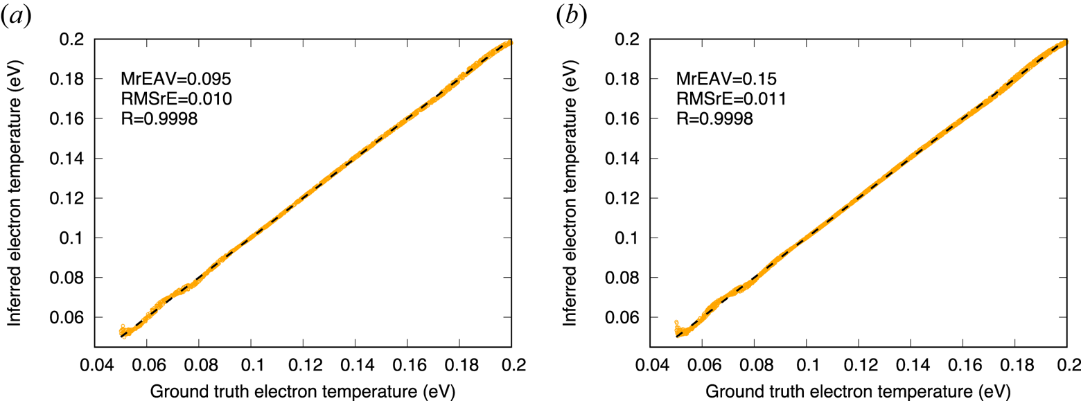
Figure 2. Correlation plot of inferred electron temperatures against known values from the training set (a), and the test set (b), for a non-emissive Langmuir probe (LP).
3.1.3. Plasma potential inferences
The simulations used to construct our solution library only account for a probe at different voltages $V$ with respect to the background plasma, without accounting for the presence of a vacuum chamber or a spacecraft to which it is attached (see the definition of $\phi$
 in (2.1)). As explained in 2.3, our simulations can be used to construct data sets with currents collected as a function of bias voltage $V_b$
 relative to the ground at different voltages $V_s$
 relative to surrounding plasma, by using (2.9). Thus for a sufficiently long probe, for which the collected current as a function of voltage $V$
 is approximately independent of the proximity to other objects, and for which end effects are negligible, it is possible to use (2.9) to construct data sets containing $I\unicode{x2013}V_b$
 characteristics for different electron densities, temperatures and plasma potentials. Here, as for the inference model considered in § 3.1.2, it is important to normalize currents in order to reduce the strong density dependence of collected currents. A method found to produce good results consists, for each characteristic, of subtracting the mean current $\langle I \rangle$
 from the entire characteristic currents, and dividing the result by $\langle I \rangle$
 . With this normalization, the resulting characteristics are only mildly dependent on the density and temperature, and they differ mostly due to the different plasma potentials. Here, given the relatively small interval of plasma potentials considered ($-2$
 to $+4$
 V), the maximum absolute error is used as a cost function. Correlation plots of the inferred, against known plasma potentials from the training (a) and test (b) sets are shown in figure 3. The plots show excellent agreement between inferred potentials and known values for both training and test sets, with nearly the same skill metrics. In both cases, the MEAV is about 0.1 V, and the RMS error, $0.048$
 V, which correspond respectively $1.7$
 % and $0.8$
 % of the 6 V range considered.

Figure 3. Correlation plot of inferred plasma potential against known values from the training set (a), and the test set (b), for a non-emissive Langmuir probe (LP).
3.2. Inferences with EP characteristics
Emissive probes are mostly used to infer plasma potentials, owing to their stronger sensitivity to that parameter (Kemp & Sellen Reference Kemp and Sellen1966; Smith, Hershkowitz & Coakley Reference Smith, Hershkowitz and Coakley1979; Sheehan & Hershkowitz Reference Sheehan and Hershkowitz2011). Our regression approach has been applied to infer the plasma temperature and density from EP characteristics, but it was not possible to obtain results with satisfactory accuracy. We therefore limit our attention to inferences of the plasma potential only. Inferences were made with RBF using the same number of centres (five) and interpolation function $G(\bar {X})$ as for non-emissive probe in § 3.1. In this case, considering that characteristics depend most strongly on the plasma potential, no normalization of the probe floating potentials is needed. The inference model is constructed by minimizing the maximum absolute error, as described in § 3. Here, considering that the plasma potential can change sign, and be close to zero, the model was constructed by minimizing the maximum absolute error between inferred and known values of $V_s$
 , as described in § 3.
Correlation plots of inferred plasma potentials against known potentials from the data set, are shown in figure 4, for training (a) and test (b). The correlation coefficients $R$ , and the RMS errors are found to be similar in both cases, with inferences being slightly less accurate for the test set. The uncertainties of $0.22$
 and $0.26$
 V for the training and test correspond respectively to $3.7$
 % and $4.3$
 % of the full 6 V range considered. These are approximately a factor two larger than those found with LP characteristics, but they nonetheless show excellent inference skill for plasma potential inferences.

Figure 4. Correlation plot of inferred plasma potential against known values from the training set (a), and the test set (b), for an emissive Langmuir probe (EP).
4. Summary and conclusion
A new approach is presented to infer space plasma parameters from long cylindrical probe characteristics in a Maxwellian plasma at rest, using a combination of kinetic simulations and multivariate regression techniques. Two types of probes are considered. One is a non-emissive Langmuir probe (LP) for which characteristics consist of $n$ -tuples of currents collected by probes for $n$
 -tuples of bias voltages. The second is an emissive probe (EP) for which the characteristics are probe floating potentials as a function of probe temperatures; both being parameterized in terms of $n$
 -tuples. Currents collected by an LP as a function of bias voltages, and floating probe potentials as a function of probe temperatures for an EP, are calculated numerically for different space environment conditions, using the OMT (numerical solutions of the Vlasov–Poisson system). The resulting characteristics are used to construct a solution library, or synthetic data set, consisting of discretized currents and corresponding bias voltages, followed by the electron density, temperature and assumed plasma potential.
When considering an LP, the range and resolution of bias voltages in the characteristics is chosen so as to cover part of the ion and electron saturation regions, while providing a sufficiently detailed representation of the electron transition region for the ranges of the assumed electron temperatures and plasma potentials. Using radial basis function regression, the inference of plasma density is mostly sensitive to the magnitude of the current collected in the electron saturation region, which does not require currents to be normalized in order to obtain good inferences. For the plasma potential and of the electron temperature, however, inferences depend more sensitively on the electron transition region, which requires adapted transformations of the current characteristics, in order to obtain good accuracy. With EPs, probe characteristics are most sensitive to the background plasma potential, and they are relatively insensitive to the density or temperature. In this case, only inferences made for the plasma potentials were found to be of satisfactory accuracy, without requiring any normalization of transformation of the characteristics.
Given plasma conditions, the direct computation of currents collected by a probe or an emissive floating potential, is a straightforward exercise with present computing resources, even if it can be somewhat time consuming. The inverse problem consisting of inferring plasma conditions from measured characteristics, however, is significantly more difficult, and it cannot be solved in real time with simulations. This would indeed require multiple simulations in which plasma parameters would be optimized so as to best fit each characteristic. While possible for a few characteristics, such an iterative approach would be impractical in actual data processing. However, the use of multivariate regressions with pre-calculated synthetic data sets offers a powerful and practical alternative for doing such inferences for data analysis. This approach, based on standard machine learning procedures, would have the added advantage of providing uncertainty margins specifically associated with the inference technique; something that is not obtained when using inference techniques based on analytic or semi-analytic expressions. To conclude, the analysis presented here is arguably based on several simplifications, but it is sufficient to demonstrate the potential of the approach presented to complement existing analytic techniques and improve plasma parameter inferences. More work will be needed for simulation-regression approaches to be adopted and applied routinely in lab and space plasmas; work which, we believe, should be of interest to experimentalists and modellers alike.
Acknowledgements
Editor Edward Thomas, Jr. thanks the referees for their advice in evaluating this article.
Funding
R.M. acknowledges financial support from the Natural Sciences and Engineering Research Council of Canada, and from Compute Canada. S.S. and G.S.-A. have received funding from the European Unions Horizon 2020 research and innovation programme under grant agreement No 828902 (E.T.PACK project).
Declaration of interest
The authors report no conflict of interest.


 Open access