


1. Introduction
Quasi-steady, self-organized, three-dimensional (3-D) helical kink structures known as ‘density snakes’ with poloidal and toroidal mode numbers $m=1$
and
$m=1$
and $n=1$
have been observed in the core of several tokamak plasma experiments. The term ‘snake’ refers to the sinusoidal pattern measured as the structure rotates toroidally past a stationary diagnostic. The formation can occur spontaneously due to small perturbations within the plasma core associated with impurity ions (Delgado-Aparicio et al. Reference Delgado-Aparicio2013
a,b; Gill et al. Reference Gill, Edwards, Pasini and Weller1992) or a rapid influx of cold particles due to pellet injection (Weller et al. Reference Weller, Cheetham, Edwards, Gill, Gondhalekar, Granetz, Snipes and Wesson1987). Both types of snake formation have been identified in multiple devices. These structures typically persist on time scales long compared with the energy confinement time. Interestingly, they can coexist with the sawtooth cycle, which is driven by an internal kink mode with the same helicity (
$n=1$
have been observed in the core of several tokamak plasma experiments. The term ‘snake’ refers to the sinusoidal pattern measured as the structure rotates toroidally past a stationary diagnostic. The formation can occur spontaneously due to small perturbations within the plasma core associated with impurity ions (Delgado-Aparicio et al. Reference Delgado-Aparicio2013
a,b; Gill et al. Reference Gill, Edwards, Pasini and Weller1992) or a rapid influx of cold particles due to pellet injection (Weller et al. Reference Weller, Cheetham, Edwards, Gill, Gondhalekar, Granetz, Snipes and Wesson1987). Both types of snake formation have been identified in multiple devices. These structures typically persist on time scales long compared with the energy confinement time. Interestingly, they can coexist with the sawtooth cycle, which is driven by an internal kink mode with the same helicity ( $m/n = 1/1$
). Similar 3-D helical states have been investigated in several other contexts within the toroidal plasma literature. Three-dimensional equilibria in the form of a saturated internal kink have been identified as lower energy configurations of tokamak plasmas (Cooper et al. Reference Cooper2013). In reversed-field pinch plasmas, the single-helical-axis and quasi-single-helicity states have been studied extensively (Marrelli et al. Reference Marrelli, Martin, Puiatti, Sarff, Chapman, Drake, Escande and Masamune2021), where the helicity corresponds to the central safety factor (e.g.
$m/n = 1/1$
). Similar 3-D helical states have been investigated in several other contexts within the toroidal plasma literature. Three-dimensional equilibria in the form of a saturated internal kink have been identified as lower energy configurations of tokamak plasmas (Cooper et al. Reference Cooper2013). In reversed-field pinch plasmas, the single-helical-axis and quasi-single-helicity states have been studied extensively (Marrelli et al. Reference Marrelli, Martin, Puiatti, Sarff, Chapman, Drake, Escande and Masamune2021), where the helicity corresponds to the central safety factor (e.g. $m/n = 1/5$
in the Madison Symmetric Torus, MST). Saturated, 3-D interchange mode structures have also been proposed to produce a ‘flux-pumping’ mechanism (akin to a dynamo) that can explain the stationary non-sawtoothing ‘hybrid’ mode observed in several tokamaks (Jardin, Ferraro & Krebs Reference Jardin, Ferraro and Krebs2015; Piovesan et al. Reference Piovesan2016, Reference Piovesan2017). Finally, quasi-steady 3-D helical structures have been observed in ultra-low-
$m/n = 1/5$
in the Madison Symmetric Torus, MST). Saturated, 3-D interchange mode structures have also been proposed to produce a ‘flux-pumping’ mechanism (akin to a dynamo) that can explain the stationary non-sawtoothing ‘hybrid’ mode observed in several tokamaks (Jardin, Ferraro & Krebs Reference Jardin, Ferraro and Krebs2015; Piovesan et al. Reference Piovesan2016, Reference Piovesan2017). Finally, quasi-steady 3-D helical structures have been observed in ultra-low- $q$
discharges with edge safety factor
$q$
discharges with edge safety factor $0 \lt q(a) \lt 1$
(Hurst et al. Reference Hurst2022; Zuin et al. Reference Zuin2022). This motivates further studies of density snakes, with the goal of understanding the spontaneous bifurcation of toroidally symmetric plasmas into 3-D helical states, and the subsequent stability and robustness of such states.
$0 \lt q(a) \lt 1$
(Hurst et al. Reference Hurst2022; Zuin et al. Reference Zuin2022). This motivates further studies of density snakes, with the goal of understanding the spontaneous bifurcation of toroidally symmetric plasmas into 3-D helical states, and the subsequent stability and robustness of such states.
Snakes were first identified within the JET experiment after an injected pellet ablated near or on the $q=1$
surface, as inferred from measurements of the sawtooth inversion radius (Weller et al. Reference Weller, Cheetham, Edwards, Gill, Gondhalekar, Granetz, Snipes and Wesson1987), where
$q=1$
surface, as inferred from measurements of the sawtooth inversion radius (Weller et al. Reference Weller, Cheetham, Edwards, Gill, Gondhalekar, Granetz, Snipes and Wesson1987), where $q$
is the safety factor. The leading theory was that the new pellet material created a localized region of depressed temperature, increasing the resistivity, which then led to a magnetic island encompassing the snake (Gill et al. Reference Gill, Edwards, Pasini and Weller1992). A typical snake persisted through much of the discharge, surviving multiple sawtooth crashes. A second process of snake formation was later observed within JET. Instead of pellet ablation, heavy impurity ions accumulated to create the local temperature drop. These impurities are either deposited onto the
$q$
is the safety factor. The leading theory was that the new pellet material created a localized region of depressed temperature, increasing the resistivity, which then led to a magnetic island encompassing the snake (Gill et al. Reference Gill, Edwards, Pasini and Weller1992). A typical snake persisted through much of the discharge, surviving multiple sawtooth crashes. A second process of snake formation was later observed within JET. Instead of pellet ablation, heavy impurity ions accumulated to create the local temperature drop. These impurities are either deposited onto the $q=1$
surface during a sawtooth event, or accumulated within the plasma core during startup. Both types of snakes have been observed in many experiments, including ASDEX (Naujoks et al. Reference Naujoks1996), Doublet III (Jahns et al. Reference Jahns, Ejima, Groebner, Brooks, Fisher, Hsieh, Taylor, Wesley, Fujisawa and Sugawara1982), Tore Supra (Pecquet et al. Reference Pecquet, Cristofani, Mattioli, Garbet, Laurent, Geraud, Gil, Joffrin and Sabot1997), PBX (Ida et al. Reference Ida, Fonck, Hulse and Leblanc1986) and EAST (Yao et al. Reference Yao, Hu, Xu, Xu, Chen and Li2016).
$q=1$
surface during a sawtooth event, or accumulated within the plasma core during startup. Both types of snakes have been observed in many experiments, including ASDEX (Naujoks et al. Reference Naujoks1996), Doublet III (Jahns et al. Reference Jahns, Ejima, Groebner, Brooks, Fisher, Hsieh, Taylor, Wesley, Fujisawa and Sugawara1982), Tore Supra (Pecquet et al. Reference Pecquet, Cristofani, Mattioli, Garbet, Laurent, Geraud, Gil, Joffrin and Sabot1997), PBX (Ida et al. Reference Ida, Fonck, Hulse and Leblanc1986) and EAST (Yao et al. Reference Yao, Hu, Xu, Xu, Chen and Li2016).
Snake formation due to impurity accumulation was further characterized in the Alcator C-Mod device with a high resolution soft X-ray diagnostic (Delgado-Aparicio et al. Reference Delgado-Aparicio2013
a, b). These measurements provided a key view of the snake throughout its life cycle. Rather than the instantaneous island, as previously proposed, the snake began gradually as an $m/n = 1/1$
helical kink mode, then slowly evolved into an island-like crescent as the minor radius of the
$m/n = 1/1$
helical kink mode, then slowly evolved into an island-like crescent as the minor radius of the $q=1$
magnetic surface,
$q=1$
magnetic surface, $r_1$
, increases. The snake then persisted through the sawtooth cycle, with each sawtooth crash slightly perturbing its rotation speed and radial size. The snake island structure was high in impurity content and lower in temperature, surrounding a low impurity, high temperature core within the crescent. During the sawtooth crash, it was found that this high temperature core moves outward radially away from the island.
$r_1$
, increases. The snake then persisted through the sawtooth cycle, with each sawtooth crash slightly perturbing its rotation speed and radial size. The snake island structure was high in impurity content and lower in temperature, surrounding a low impurity, high temperature core within the crescent. During the sawtooth crash, it was found that this high temperature core moves outward radially away from the island.
Numerical modeling work was done to better characterize the internal structure of these snakes as they evolve and interact with the sawtooth cycle (Sugiyama Reference Sugiyama2013). The simulations showed that the region of enhanced density inside the snake coincides with a low temperature region in the core, causing the pressure gradient to remain small, maintaining magnetohydrodynamic (MHD) force balance. If the density region lies on the low pressure side of the gradient, the displacement of the sawtooth crash occurs in a direction opposite to the snake, allowing the structure to avoid the crash. However, in the simulations this only occurred when $r_1$
was sufficiently small. When
$r_1$
was sufficiently small. When $r_1$
increased sufficiently, the density and temperature remained aligned, causing the crash to occur in the direction of the snake. After a sawtooth crash, much of the density in the snake was deposited at
$r_1$
increased sufficiently, the density and temperature remained aligned, causing the crash to occur in the direction of the snake. After a sawtooth crash, much of the density in the snake was deposited at $r \gt r_1$
, significantly decreasing the density perturbation. It was suggested that there may be a minimum density requirement for snakes to persist through a sawtooth crash in the large
$r \gt r_1$
, significantly decreasing the density perturbation. It was suggested that there may be a minimum density requirement for snakes to persist through a sawtooth crash in the large $r_1$
case, although those cases were not simulated in the study.
$r_1$
case, although those cases were not simulated in the study.
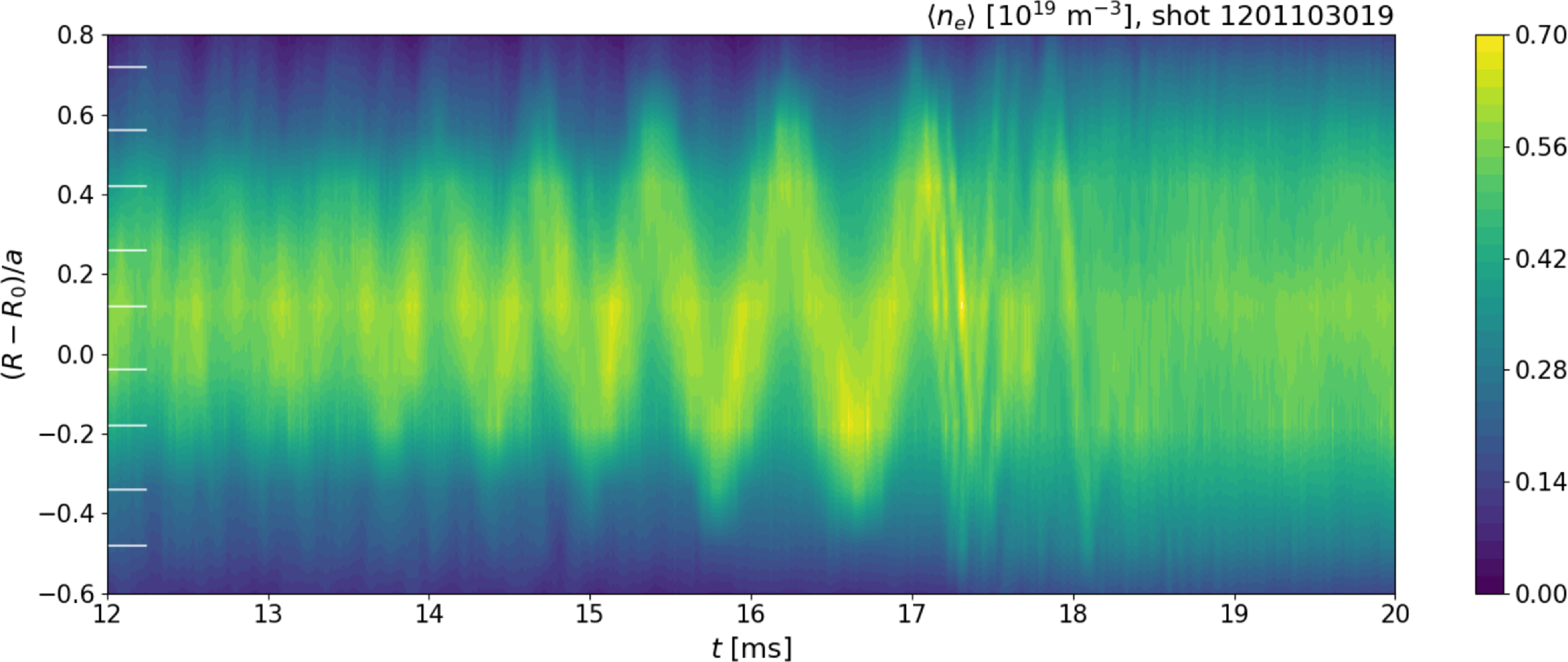
Figure 1. A typical density snake measured by the 11-chord interferometer in an MST tokamak plasma with edge safety factor $q(a) = 2.3$
. The color map is interpolated between chords that sample the line-integrated electron density
$q(a) = 2.3$
. The color map is interpolated between chords that sample the line-integrated electron density $\langle n_e \rangle$
at major radial locations
$\langle n_e \rangle$
at major radial locations $R$
indicated by white tick marks along the vertical axis, where
$R$
indicated by white tick marks along the vertical axis, where $R_0$
and
$R_0$
and $a$
are the major and minor radii of the device. The oscillation is distinguishable roughly in the time span
$a$
are the major and minor radii of the device. The oscillation is distinguishable roughly in the time span $14 \lt t \lt 17.5$
ms, after which it loses coherence due to its interaction with a sawtooth crash. Here, q(a) = 2.35.
$14 \lt t \lt 17.5$
ms, after which it loses coherence due to its interaction with a sawtooth crash. Here, q(a) = 2.35.
Recently, density snakes have been observed in ohmically heated tokamak plasmas in the MST device with relatively low edge safety factor $q(a)\gtrsim 2.2$
. They are clearly detected using an interferometer diagnostic measuring line-integrated electron density along 11 vertical chords spanning most of the major radial extent of the plasma. An example of interferometer data showing a typical density snake is shown in figure 1. The helical structure rotates toroidally past the fixed diagnostic, yielding a snake-like sinusoidal pattern in the data. Data from an internal magnetic probe, edge magnetic coils and impurity ion spectroscopy also show evidence of the helical structures consistent with that from the interferometer. Preliminary modeling suggests the internal structure of MST snakes is closer to a saturated resistive kink mode with a large magnetic island, rather than an ideal kink or the crescent-shaped snakes seen in Alcator C-Mod. The snakes observed so far in MST typically form early in the discharges, when diffusive current peaking has proceeded such that the core safety factor is near unity. They form spontaneously and not in a repeatable way, possibly due to accumulation of impurities in the core. On average, they last for a few rotation cycles before they are destroyed by a sawtooth crash. They occupy a broader extent of the plasma minor radius and are less robust to perturbations than those studied in other devices, likely due to the low value of
$q(a)\gtrsim 2.2$
. They are clearly detected using an interferometer diagnostic measuring line-integrated electron density along 11 vertical chords spanning most of the major radial extent of the plasma. An example of interferometer data showing a typical density snake is shown in figure 1. The helical structure rotates toroidally past the fixed diagnostic, yielding a snake-like sinusoidal pattern in the data. Data from an internal magnetic probe, edge magnetic coils and impurity ion spectroscopy also show evidence of the helical structures consistent with that from the interferometer. Preliminary modeling suggests the internal structure of MST snakes is closer to a saturated resistive kink mode with a large magnetic island, rather than an ideal kink or the crescent-shaped snakes seen in Alcator C-Mod. The snakes observed so far in MST typically form early in the discharges, when diffusive current peaking has proceeded such that the core safety factor is near unity. They form spontaneously and not in a repeatable way, possibly due to accumulation of impurities in the core. On average, they last for a few rotation cycles before they are destroyed by a sawtooth crash. They occupy a broader extent of the plasma minor radius and are less robust to perturbations than those studied in other devices, likely due to the low value of $q(a)$
. As
$q(a)$
. As $q(a)$
is increased up to 3.2, the snakes have smaller minor radial extent and are more likely to survive through sawtooth crashes, although significant changes to their characteristics are observed during these interactions.
$q(a)$
is increased up to 3.2, the snakes have smaller minor radial extent and are more likely to survive through sawtooth crashes, although significant changes to their characteristics are observed during these interactions.
This paper is structured in the following way: in § 2, a discussion of the MST experiment and the diagnostics and numerical routines used for identifying and characterizing snakes is given. In § 3.1, measurements and characteristics of snake structures in quasi-steady conditions are presented. In § 3.2 the interferometer data are compared with several simple models of kink-like density perturbations. In § 3.3, data are presented regarding transient changes to snake properties, e.g. during initial growth or during interactions with sawtooth crashes. In § 4, a discussion of the results is provided, including how they relate to the findings to prior experiments. Finally, § 5 contains a summary and conclusions of the work and describes ideas for future endeavors.
2. Experimental set-up and methods
The MST is an axisymmetric toroidal magnetic confinement plasma device with circular cross-section and major radius $R=1.5$
m. It is capable of both reversed-field pinch and low-field (
$R=1.5$
m. It is capable of both reversed-field pinch and low-field ( $B \leqslant 0.14$
T) tokamak operation (Dexter et al. Reference Dexter, Kerst, Lovell, Prager and Sprott1991). The MST features a close-fitting 5-cm-thick aluminum shell with minor radius
$B \leqslant 0.14$
T) tokamak operation (Dexter et al. Reference Dexter, Kerst, Lovell, Prager and Sprott1991). The MST features a close-fitting 5-cm-thick aluminum shell with minor radius $a=0.52\,\rm m$
. Insulated cuts in the shell allow the magnetic field to enter the chamber. Graphite limiters mounted on the inside surface define a plasma with a minor radius of
$a=0.52\,\rm m$
. Insulated cuts in the shell allow the magnetic field to enter the chamber. Graphite limiters mounted on the inside surface define a plasma with a minor radius of $b=0.50$
m. The shell has a resistive wall time constant of
$b=0.50$
m. The shell has a resistive wall time constant of $\tau _w = 800\,\rm ms$
that maintains a small radial magnetic field at the plasma surface and inhibits the formation of ideal external kinks over the typical plasma duration of 50 ms
$\tau _w = 800\,\rm ms$
that maintains a small radial magnetic field at the plasma surface and inhibits the formation of ideal external kinks over the typical plasma duration of 50 ms $\lt \lt \tau _w$
. Both the toroidal field,
$\lt \lt \tau _w$
. Both the toroidal field, $B_{\phi }$
, and plasma current,
$B_{\phi }$
, and plasma current, $I_p$
, are produced by feedback-controlled programmable power supplies that use pulse-width modulation with a 10 kHz carrier frequency to meet arbitrary demand waveforms (Holly et al. Reference Holly, Chapman, McCollam and Morin2015). The only heating mechanism utilized in this study was ohmic heating from the plasma current. In the experiments presented here,
$I_p$
, are produced by feedback-controlled programmable power supplies that use pulse-width modulation with a 10 kHz carrier frequency to meet arbitrary demand waveforms (Holly et al. Reference Holly, Chapman, McCollam and Morin2015). The only heating mechanism utilized in this study was ohmic heating from the plasma current. In the experiments presented here, $B_{\phi }$
,
$B_{\phi }$
, $I_p$
and therefore
$I_p$
and therefore $q(a) \propto B_{\phi }/I_p$
are held constant throughout each discharge, but
$q(a) \propto B_{\phi }/I_p$
are held constant throughout each discharge, but $I_p$
is varied between discharges to investigate the dependence of snake behavior on
$I_p$
is varied between discharges to investigate the dependence of snake behavior on $q(a)$
. Interestingly, MST is capable of routine, non-disruptive operation at low safety factor
$q(a)$
. Interestingly, MST is capable of routine, non-disruptive operation at low safety factor $q(a) \lt 2$
due to the thick, close-fitting, conductive wall (Hurst et al. Reference Hurst2022). This builds upon prior results from DIII-D (Piovesan et al. Reference Piovesan2014) and RFX-Mod (Zanca et al. Reference Zanca, Paccagnella, Finotti, Fassina, Manduchi, Cavazzana, Franz, Piron and Piron2015) in which active magnetic feedback was used to suppress the
$q(a) \lt 2$
due to the thick, close-fitting, conductive wall (Hurst et al. Reference Hurst2022). This builds upon prior results from DIII-D (Piovesan et al. Reference Piovesan2014) and RFX-Mod (Zanca et al. Reference Zanca, Paccagnella, Finotti, Fassina, Manduchi, Cavazzana, Franz, Piron and Piron2015) in which active magnetic feedback was used to suppress the $m=2$
,
$m=2$
, $n=1$
resistive wall mode. The ranges of plasma parameters for the data presented here are shown in table 1, where
$n=1$
resistive wall mode. The ranges of plasma parameters for the data presented here are shown in table 1, where $q(a)$
is near but not below 2 throughout the dataset. Of particular note, the electron temperature in these discharges is lower (and resistivity higher) than in many previous snake studies.
$q(a)$
is near but not below 2 throughout the dataset. Of particular note, the electron temperature in these discharges is lower (and resistivity higher) than in many previous snake studies.
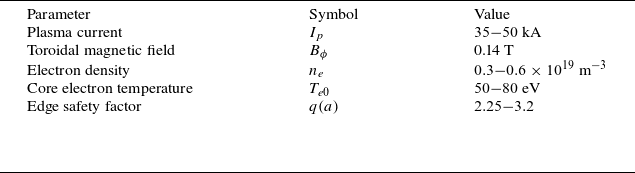
Table 1. Range of plasma parameters used for the density snake experiments described here. Electron temperature is an estimate based on data gathered in other similar discharges in MST (Hurst et al. Reference Hurst2022).
The density snakes are primarily diagnosed using the interferometer system described above with 11 vertical chords spanning most of the major radial extent of the plasma from $R =$
1.18 to 1.93 m (Parke et al. Reference Parke, Ding, Duff and Brower2016), where five of the chords are offset by
$R =$
1.18 to 1.93 m (Parke et al. Reference Parke, Ding, Duff and Brower2016), where five of the chords are offset by $5^{\circ }$
toroidally from the other six. It is not sensitive to motion of the snake structure in the vertical direction
$5^{\circ }$
toroidally from the other six. It is not sensitive to motion of the snake structure in the vertical direction $Z$
, but the spatial resolution in
$Z$
, but the spatial resolution in $R$
provides a powerful constraint on the snake structure and dynamics. The interferometer signals feature low-frequency noise of the order of
$R$
provides a powerful constraint on the snake structure and dynamics. The interferometer signals feature low-frequency noise of the order of $\langle n_e \rangle \sim 0.05 \times 10^{19}$
, which is relatively unimportant for the large density perturbations associated with the snakes, but limits the ability to accurately measure small densities near the plasma edge. Several other diagnostics are also used to better understand the snake structure and behavior. Edge toroidal and poloidal magnetic pickup coil arrays provide spectral information regarding magnetic fluctuations at the plasma surface with
$\langle n_e \rangle \sim 0.05 \times 10^{19}$
, which is relatively unimportant for the large density perturbations associated with the snakes, but limits the ability to accurately measure small densities near the plasma edge. Several other diagnostics are also used to better understand the snake structure and behavior. Edge toroidal and poloidal magnetic pickup coil arrays provide spectral information regarding magnetic fluctuations at the plasma surface with $m \leqslant 7$
and
$m \leqslant 7$
and $n \leqslant 15$
. A deep-insertion magnetic probe measures internal three-axis magnetic fields at radial locations
$n \leqslant 15$
. A deep-insertion magnetic probe measures internal three-axis magnetic fields at radial locations $r/a \gt 0.66$
with spatial resolution of 1 cm. Finally, impurity ion radiation and temperature are measured using a high-throughput dual-grating spectrometer. It views the plasma along two chords, one of which is aligned with the magnetic axis and the other with a tangency radius
$r/a \gt 0.66$
with spatial resolution of 1 cm. Finally, impurity ion radiation and temperature are measured using a high-throughput dual-grating spectrometer. It views the plasma along two chords, one of which is aligned with the magnetic axis and the other with a tangency radius $r/a = 0.45$
(Craig et al. Reference Craig, Den Hartog, Ennis, Gangadhara and Holly2007). Boron-IV line emissions at
$r/a = 0.45$
(Craig et al. Reference Craig, Den Hartog, Ennis, Gangadhara and Holly2007). Boron-IV line emissions at $\lambda = 282$
nm with a resolution of
$\lambda = 282$
nm with a resolution of $\lambda / \delta \lambda = 5600$
were primarily used for this work. The geometry of these diagnostics in the poloidal plane is shown schematically in figure 2.
$\lambda / \delta \lambda = 5600$
were primarily used for this work. The geometry of these diagnostics in the poloidal plane is shown schematically in figure 2.
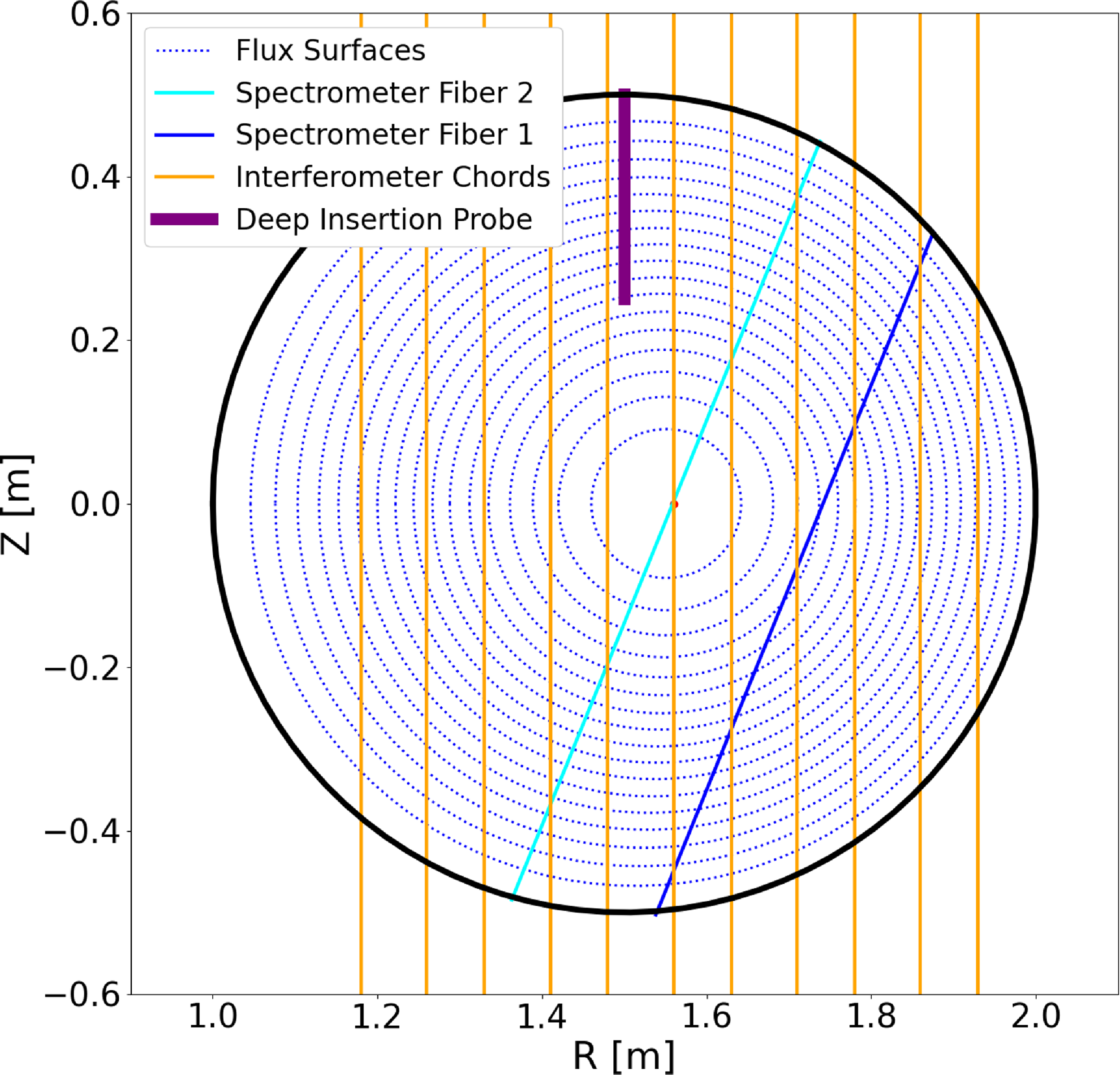
Figure 2. Geometry of diagnostics used in the experiments presented here, projected onto the poloidal plane. Lines corresponding to the inteferometer and spectrometer diagnostics represent viewing chords over which the signal is integrated, whereas the deep-insertion probe line represents the span of multiple localized measurements. The spectrometer is located at toroidal angle $270^{\circ }$
relative to the poloidal cut in the shell; five of the interferometer chords at
$270^{\circ }$
relative to the poloidal cut in the shell; five of the interferometer chords at $250^{\circ }$
and the other six at
$250^{\circ }$
and the other six at $255^{\circ }$
; and the deep-insertion probe at
$255^{\circ }$
; and the deep-insertion probe at $300^{\circ }$
. Magnetic flux surfaces are computed with the MSTFit toroidal equilibrium reconstruction code (Anderson et al. Reference Anderson, Forest, Biewer, Sarff and Wright2004), and the solid black line indicates the inner surface of the vacuum shell.
$300^{\circ }$
. Magnetic flux surfaces are computed with the MSTFit toroidal equilibrium reconstruction code (Anderson et al. Reference Anderson, Forest, Biewer, Sarff and Wright2004), and the solid black line indicates the inner surface of the vacuum shell.
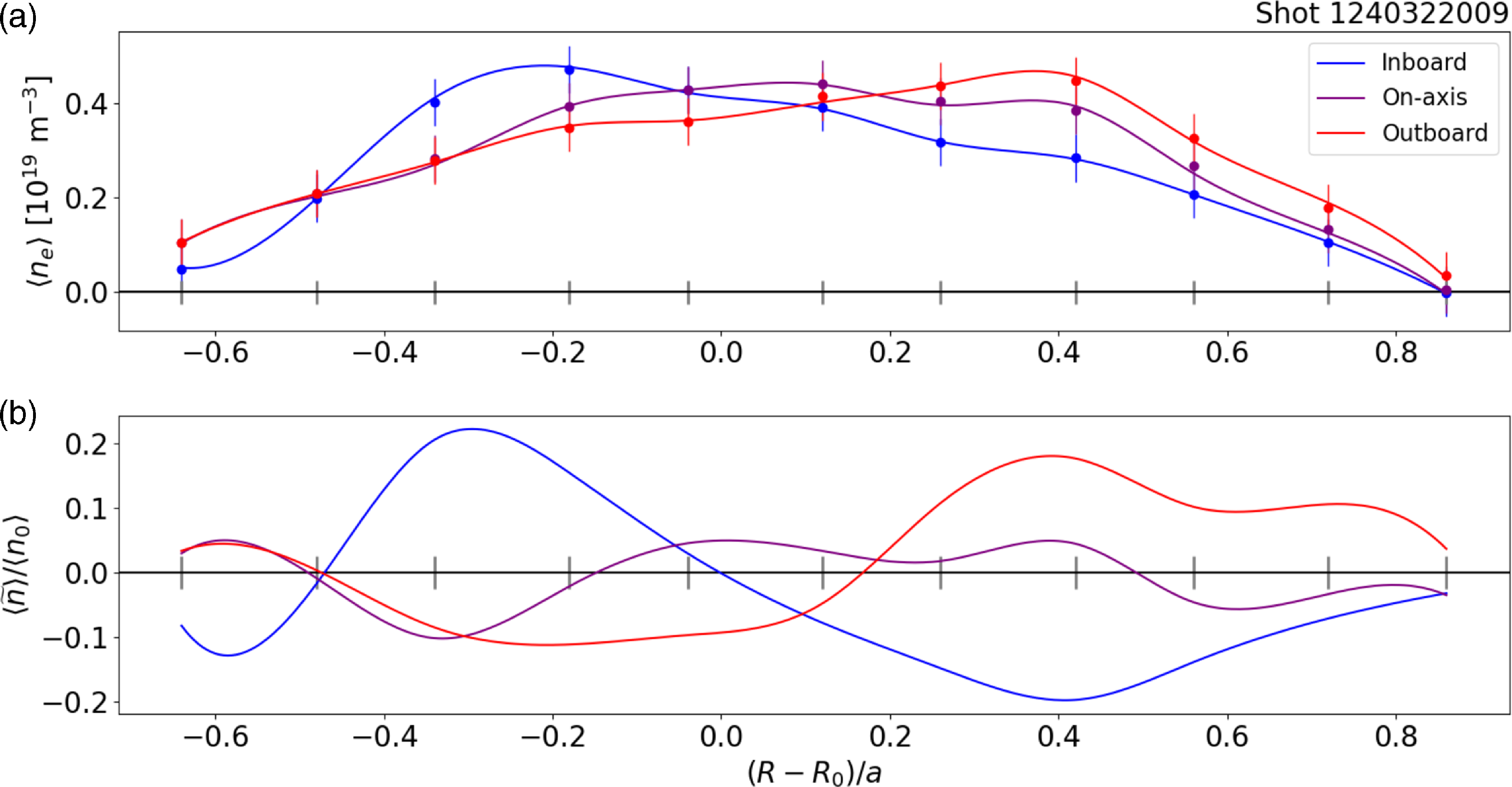
Figure 3. Major radial profiles of the interferometer data at three points in time corresponding to phases in the snake rotation where the helical core is located farthest inboard, farthest outboard and near the axis. Shown are (a) the individual chord measurements and interpolated curves, and (b) the density perturbation obtained by subtracting the time-averaged signal as described in the text. Here, q(a) = 2.3.
A numerical algorithm was developed to identify density snakes and extract their characteristics from the line-integrated interferometer data, $\langle n_e \rangle (R,t)$
. At each point in time, the algorithm interpolates the data over the
$\langle n_e \rangle (R,t)$
. At each point in time, the algorithm interpolates the data over the $R$
-coordinate, finds the maximum of
$R$
-coordinate, finds the maximum of $\langle n_e \rangle (R)$
and its location
$\langle n_e \rangle (R)$
and its location $R_{{max}}$
and finds the inboard and outboard
$R_{{max}}$
and finds the inboard and outboard $R$
-locations at which the signal is 85 % of the maximum. This threshold was chosen based on typical observed values of the density perturbation across a wide range of snake events, and by checking the results against visual inspection with different threshold values. An example of the line-averaged density along each chord is given in figure 3(a) at three points in time: when the helical core is located at the lowest value of
$R$
-locations at which the signal is 85 % of the maximum. This threshold was chosen based on typical observed values of the density perturbation across a wide range of snake events, and by checking the results against visual inspection with different threshold values. An example of the line-averaged density along each chord is given in figure 3(a) at three points in time: when the helical core is located at the lowest value of $R$
(inboard), the highest value (outboard), and at the value nearest that of the magnetic axis. Panel (b) shows the density perturbation
$R$
(inboard), the highest value (outboard), and at the value nearest that of the magnetic axis. Panel (b) shows the density perturbation $\langle \tilde {n}_e \rangle = \langle n_e \rangle - \langle n_{e0} \rangle$
, where
$\langle \tilde {n}_e \rangle = \langle n_e \rangle - \langle n_{e0} \rangle$
, where $ \langle n_{e0} \rangle$
is time averaged over a full cycle of snake rotation. This shows that the maximum chord-averaged density perturbation of a typical snake is around 20 % of the background density, and that the choice of the 85 % relative density contour is suitable to capture the density peak without being sensitive to lower, secondary peaks.
$ \langle n_{e0} \rangle$
is time averaged over a full cycle of snake rotation. This shows that the maximum chord-averaged density perturbation of a typical snake is around 20 % of the background density, and that the choice of the 85 % relative density contour is suitable to capture the density peak without being sensitive to lower, secondary peaks.
Carried out at each sampling time, this yields two curves in $(R,t)$
space bounding the peak of the interferometer signal, one each on the inboard and outboard side. Sine waves of the form
$(R,t)$
space bounding the peak of the interferometer signal, one each on the inboard and outboard side. Sine waves of the form $R(t) - R_0 = A \sin (f t + \Phi) + C$
are numerically fitted to each of the curves using a least-squares routine within a time window
$R(t) - R_0 = A \sin (f t + \Phi) + C$
are numerically fitted to each of the curves using a least-squares routine within a time window $t_0 - \delta t/2 \lt t \lt t_0 + \delta t/2$
. This process is repeated with
$t_0 - \delta t/2 \lt t \lt t_0 + \delta t/2$
. This process is repeated with $\delta t = 1$
ms and
$\delta t = 1$
ms and $t_0$
varying over the discharge duration, yielding optimized values and relative fit errors of the amplitudes
$t_0$
varying over the discharge duration, yielding optimized values and relative fit errors of the amplitudes $A(t)$
, rotation frequencies
$A(t)$
, rotation frequencies $f(t)$
, phase shifts
$f(t)$
, phase shifts $\Phi (t)$
and offsets
$\Phi (t)$
and offsets $C(t)$
. Density snake events are identified when there is a continuous span of time where the fit errors of the inboard and outboard amplitude and frequency are below a threshold of 10 %. Other threshold values were tested but this choice most accurately identified snakes when comparing with visual inspection. This way, the duration of each event is also extracted. The parameter ranges are restricted to
$C(t)$
. Density snake events are identified when there is a continuous span of time where the fit errors of the inboard and outboard amplitude and frequency are below a threshold of 10 %. Other threshold values were tested but this choice most accurately identified snakes when comparing with visual inspection. This way, the duration of each event is also extracted. The parameter ranges are restricted to $0.02 \lt A \lt 0.3\,\rm m$
,
$0.02 \lt A \lt 0.3\,\rm m$
, $0.5 \lt f \lt 5\,\rm kHz$
and
$0.5 \lt f \lt 5\,\rm kHz$
and $-0.3 \lt C \lt 0.3\,\rm m$
. These values are based on inspection of many events, and help to avoid false positives. The width of the snake can also be calculated as
$-0.3 \lt C \lt 0.3\,\rm m$
. These values are based on inspection of many events, and help to avoid false positives. The width of the snake can also be calculated as $W = R_+(t) - R_-(t)$
, where the subscripts
$W = R_+(t) - R_-(t)$
, where the subscripts $+/-$
label the outboard and inboard curves, respectively. Its value is dependent on the choice of the 85 % relative density contour, but it is still useful in comparing relative widths between different snake events.
$+/-$
label the outboard and inboard curves, respectively. Its value is dependent on the choice of the 85 % relative density contour, but it is still useful in comparing relative widths between different snake events.
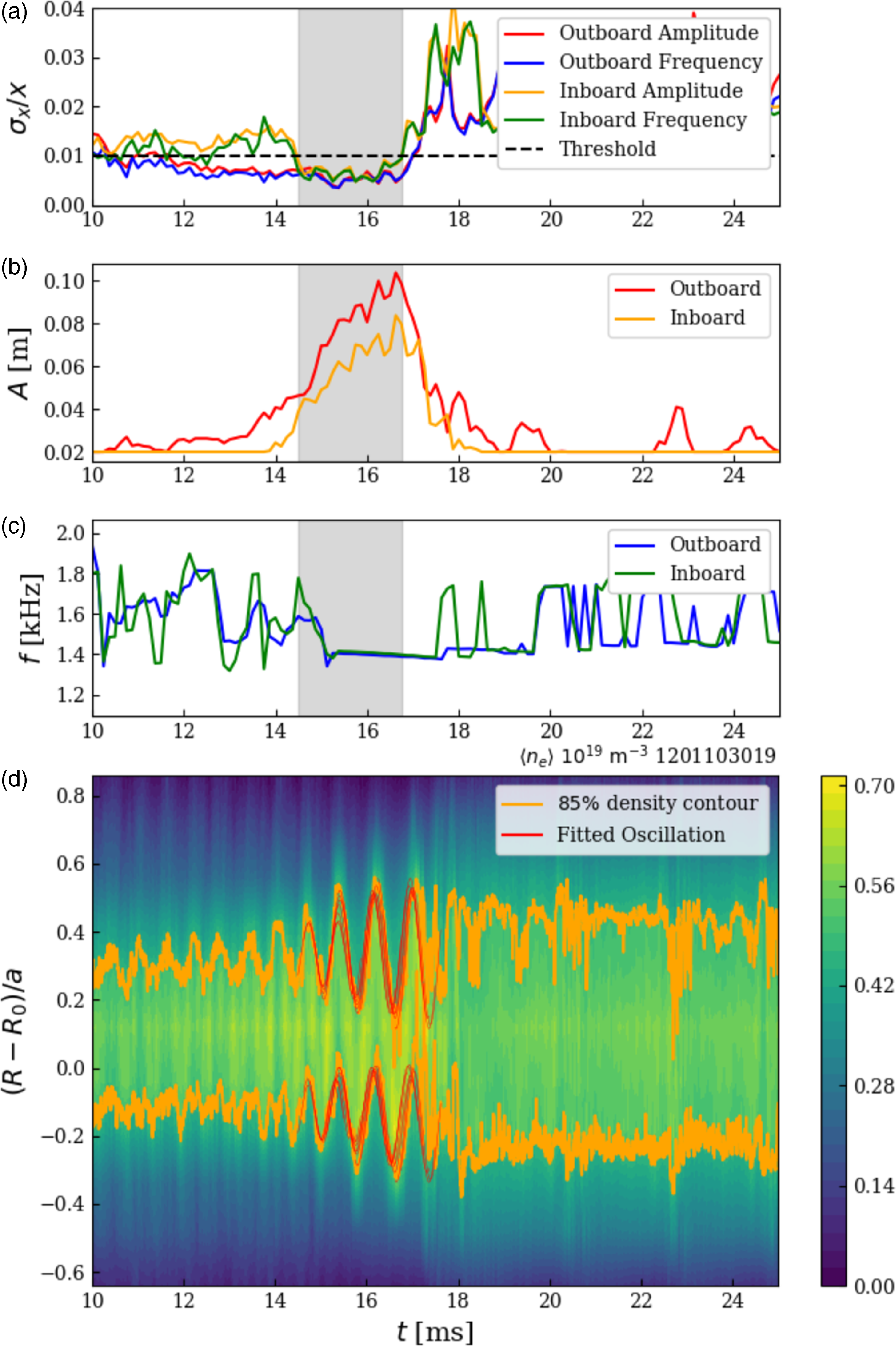
Figure 4. Example of results from the numerical algorithm for snake identification and characterization, for the same event shown in figure 1. (a) Relative error of the fit parameters $A$
or
$A$
or $f$
. The shaded regions in panels (a)–(c) indicate when the relative error is below a threshold of 10 % for all of these parameters, indicating a probable snake event. Also shown are (b) the fitted amplitude, and (c) the fitted frequency versus time. (d) The 85 % relative density contour and fitted curves are plotted over a contour map of the interferometer data. Here, q(a) = 2.35.
$f$
. The shaded regions in panels (a)–(c) indicate when the relative error is below a threshold of 10 % for all of these parameters, indicating a probable snake event. Also shown are (b) the fitted amplitude, and (c) the fitted frequency versus time. (d) The 85 % relative density contour and fitted curves are plotted over a contour map of the interferometer data. Here, q(a) = 2.35.
An example of this algorithm is given in figure 4 for the snake event shown earlier in figure 1. The inboard and outboard contours and fitted curves are plotted over a contour map of the interferometer data in panel (d), with fit parameters shown over time before, during and after the snake in panels (b) and (c). In this example, the algorithm identifies a single snake event lasting from $t = 14$
to
$t = 14$
to $17.375\,\rm ms$
, where the amplitude of the oscillation in the major radial coordinate is approximately 0.1 m and the rotation frequency is approximately 1.5 kHz. Here,
$17.375\,\rm ms$
, where the amplitude of the oscillation in the major radial coordinate is approximately 0.1 m and the rotation frequency is approximately 1.5 kHz. Here, $\sigma _x/x$
refers to the relative error for each quantity plotted in panel (a). Approximately 100 similar events were identified by eye across separate plasma discharges in MST, with 72 being identified by the algorithm.
$\sigma _x/x$
refers to the relative error for each quantity plotted in panel (a). Approximately 100 similar events were identified by eye across separate plasma discharges in MST, with 72 being identified by the algorithm.
This method is subject to a few problems that complicate snake identification and characterization. First, the thresholds for fits are based on empirical observation. Some snake events are identifiable by visual inspection, yet are not consistently captured by the algorithm. In cases where snakes survive through disturbances such as sawtooth crashes, the fit error increases temporarily and causes the algorithm to identify different events before and after the disturbance. This can be used to identify such disturbances, but makes it difficult to accurately extract the snake duration or lifetime. The $5^{\circ }$
toroidal separation between adjacent chords does not appear to significantly impact the results. In some cases, weak oscillations near the snake rotation frequency are visible prior to numerical identification of the snake, indicating a possible precursor mode involved in growth of the snake that is not captured by the routine.
$5^{\circ }$
toroidal separation between adjacent chords does not appear to significantly impact the results. In some cases, weak oscillations near the snake rotation frequency are visible prior to numerical identification of the snake, indicating a possible precursor mode involved in growth of the snake that is not captured by the routine.
3. Onset, persistence and termination of density snakes
The life cycle of a typical density snake can be broken roughly into three sections: its formation and growth, followed by saturation of the mode and a period of time where the structure is steady and its eventual termination. The structure is considered steady when its amplitude, width, rotation frequency, etc. are roughly constant in time. In most cases considered here, termination occurs abruptly and is thought to be due to interaction of the snake with a sawtooth crash. In some cases, snakes are found to survive sawtooth crashes or other perturbations, although they are usually modified in the process. In this section, we describe first the properties of steady snakes, focusing on the dependence on edge safety factor and correlation with other diagnostics. Then, we discuss the formation, termination and perturbations to the snake structures, with special consideration to their interaction with the sawtooth cycle.
3.1. Behavior in steady conditions
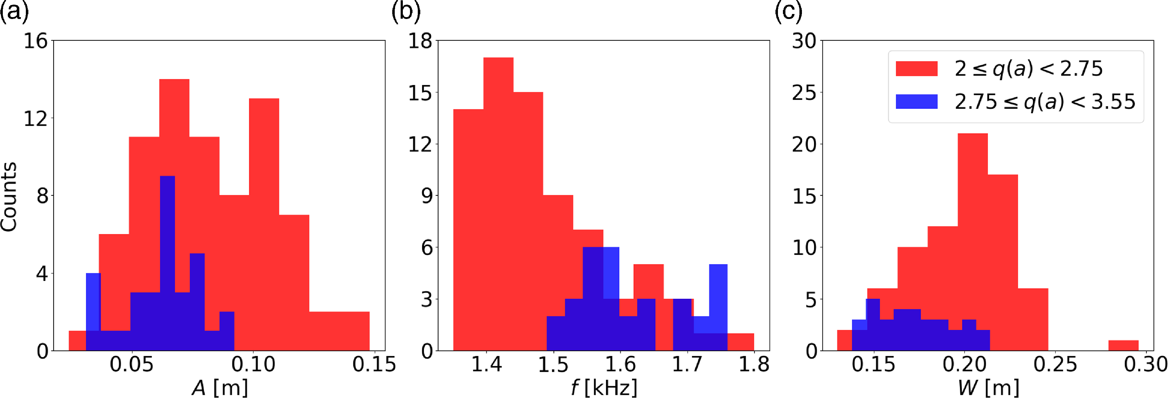
Figure 5. Histograms of snake parameters gathered using the algorithm described in § 2 for two different groupings of edge safety factor values. Shown are (a) the radial amplitude of the oscillation; (b) the rotation frequency; and (c) the width of the density perturbation at the 85 % relative density contour. As the edge safety factor increases, the amplitude and width decrease on average, while the frequency increases. In panels (a) and (b), inboard and outboard measurements are averaged together.
Density snakes are prominently observed as strong density fluctuations detected by the interferometer diagnostic. These coherent fluctuations span a large portion of the device with a significant density perturbation, with the entire structure rotating in the direction of the electron diamagnetic drift. The numerical routine described in § 2 is an important tool for gathering statistics of the snake properties and investigating their dependence on plasma parameters. This is demonstrated in figure 5, which shows the statistical distributions of amplitude, frequency and width of snake events. The typical events with $2\leqslant q(a)\lt 2.75$
analyzed using this algorithm have an average rotation frequency of approximately
$2\leqslant q(a)\lt 2.75$
analyzed using this algorithm have an average rotation frequency of approximately $f = 1.5 \pm 0.11$
kHz, an average amplitude of
$f = 1.5 \pm 0.11$
kHz, an average amplitude of $A = 0.082 \pm 0.027\,\rm m$
and a perturbation width of
$A = 0.082 \pm 0.027\,\rm m$
and a perturbation width of $W = 0.2 \pm 0.028\,\rm m$
, where the uncertainties represent standard deviations. However, these parameters depend on the variables of the plasma discharge. When
$W = 0.2 \pm 0.028\,\rm m$
, where the uncertainties represent standard deviations. However, these parameters depend on the variables of the plasma discharge. When $q(a)$
is varied, the radial safety factor profile will naturally change, causing
$q(a)$
is varied, the radial safety factor profile will naturally change, causing $r_1$
to shrink. This translates to a smaller density structure, which is consistent with the trend observed in panels (a) and (c). The average values change to
$r_1$
to shrink. This translates to a smaller density structure, which is consistent with the trend observed in panels (a) and (c). The average values change to $f = 1.6 \pm 0.082\,\rm kHz$
,
$f = 1.6 \pm 0.082\,\rm kHz$
, $A = 0.063 \pm 0.016\,\rm m$
and
$A = 0.063 \pm 0.016\,\rm m$
and $W = 0.17 \pm 0.030\,\rm m$
. The cause of the increased rotation frequency observed at higher
$W = 0.17 \pm 0.030\,\rm m$
. The cause of the increased rotation frequency observed at higher $q(a)$
may be related to the more peaked current and pressure profiles, which increases the diamagnetic drift velocity.
$q(a)$
may be related to the more peaked current and pressure profiles, which increases the diamagnetic drift velocity.
The snakes carry a significant magnetic fluctuation in addition to that of the density, which can offer insight into the mode dynamics. Using a deep-insertion probe to measure internal magnetic fields, the magnetic signal is correlated with the density fluctuation between approximately 12 and 16 ms in figure 6. The cross-correlation of the probe signal at $Z/a = 0.856$
and the interferometer signal at
$Z/a = 0.856$
and the interferometer signal at $(R-R_0)/a = 0.42$
yields a phase shift of
$(R-R_0)/a = 0.42$
yields a phase shift of $135^{\circ }$
at the snake rotation frequency of 1.33 kHz. The expected phase shift is
$135^{\circ }$
at the snake rotation frequency of 1.33 kHz. The expected phase shift is $m \Delta \theta + n \Delta \phi$
, where
$m \Delta \theta + n \Delta \phi$
, where $\Delta \theta = 90^{\circ }$
and
$\Delta \theta = 90^{\circ }$
and $\Delta \phi = 50^{\circ }$
(see figure 2). This is roughly consistent with the measured shift for
$\Delta \phi = 50^{\circ }$
(see figure 2). This is roughly consistent with the measured shift for $m/n = 1/1$
, where the positive density perturbation is associated with a positive poloidal field perturbation due to flux compression between the snake and the wall. The magnetic structure is also observed globally with the toroidal coil array, where at the edge a significant
$m/n = 1/1$
, where the positive density perturbation is associated with a positive poloidal field perturbation due to flux compression between the snake and the wall. The magnetic structure is also observed globally with the toroidal coil array, where at the edge a significant $n=1$
component dominates other modes and rotates at the same frequency as the density perturbation, as shown in figure 7.
$n=1$
component dominates other modes and rotates at the same frequency as the density perturbation, as shown in figure 7.
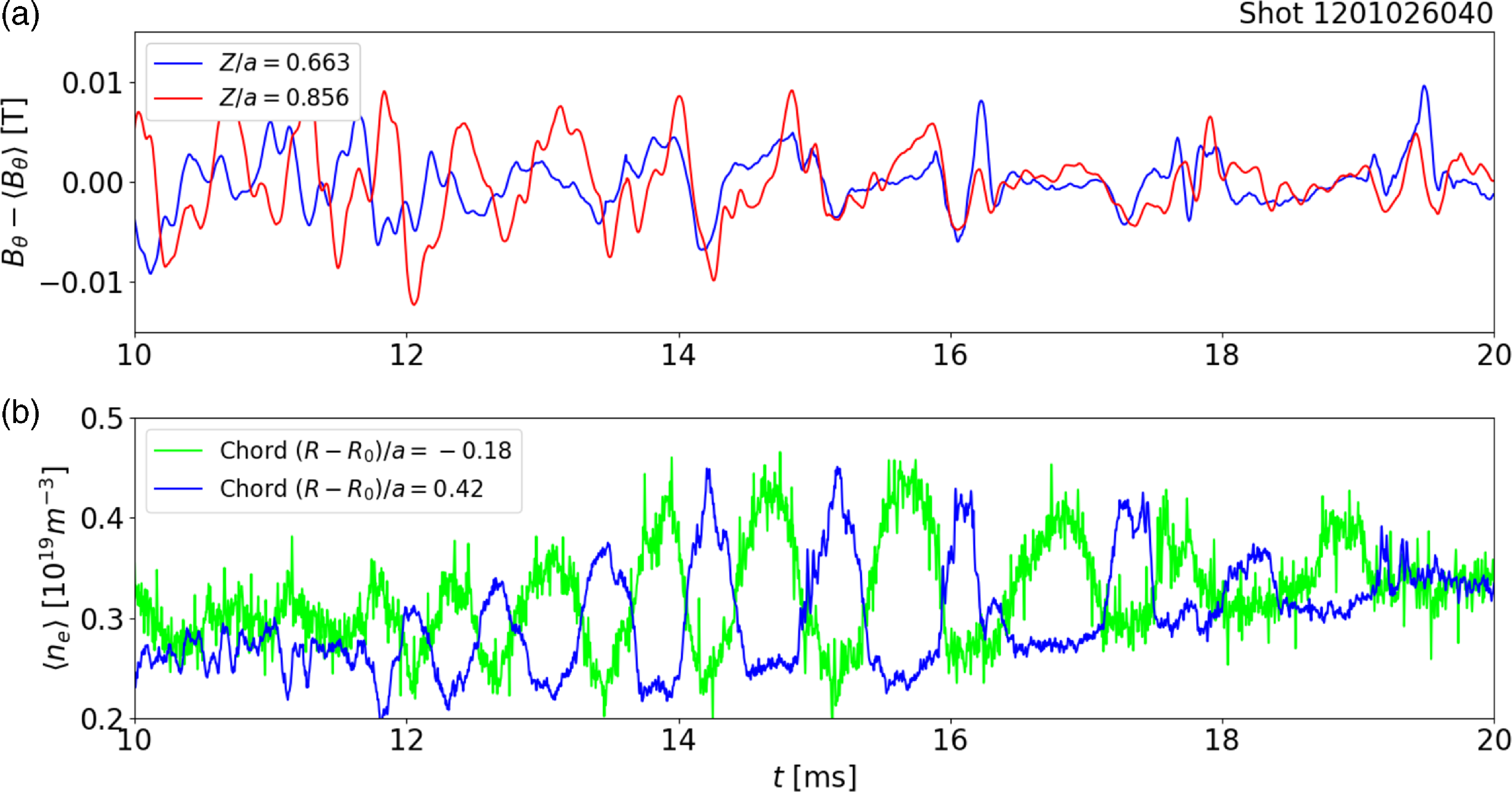
Figure 6. (a) Poloidal field perturbations taken at multiple depths using an insertable probe, and (b) data from two interferometer chords roughly equidistant from the magnetic axis. Oscillations in panel (a) are correlated with those in panel (b) as described in the text, indicating a magnetic fluctuation consistent with the snake rotation. Here, q(a) = 2.27.
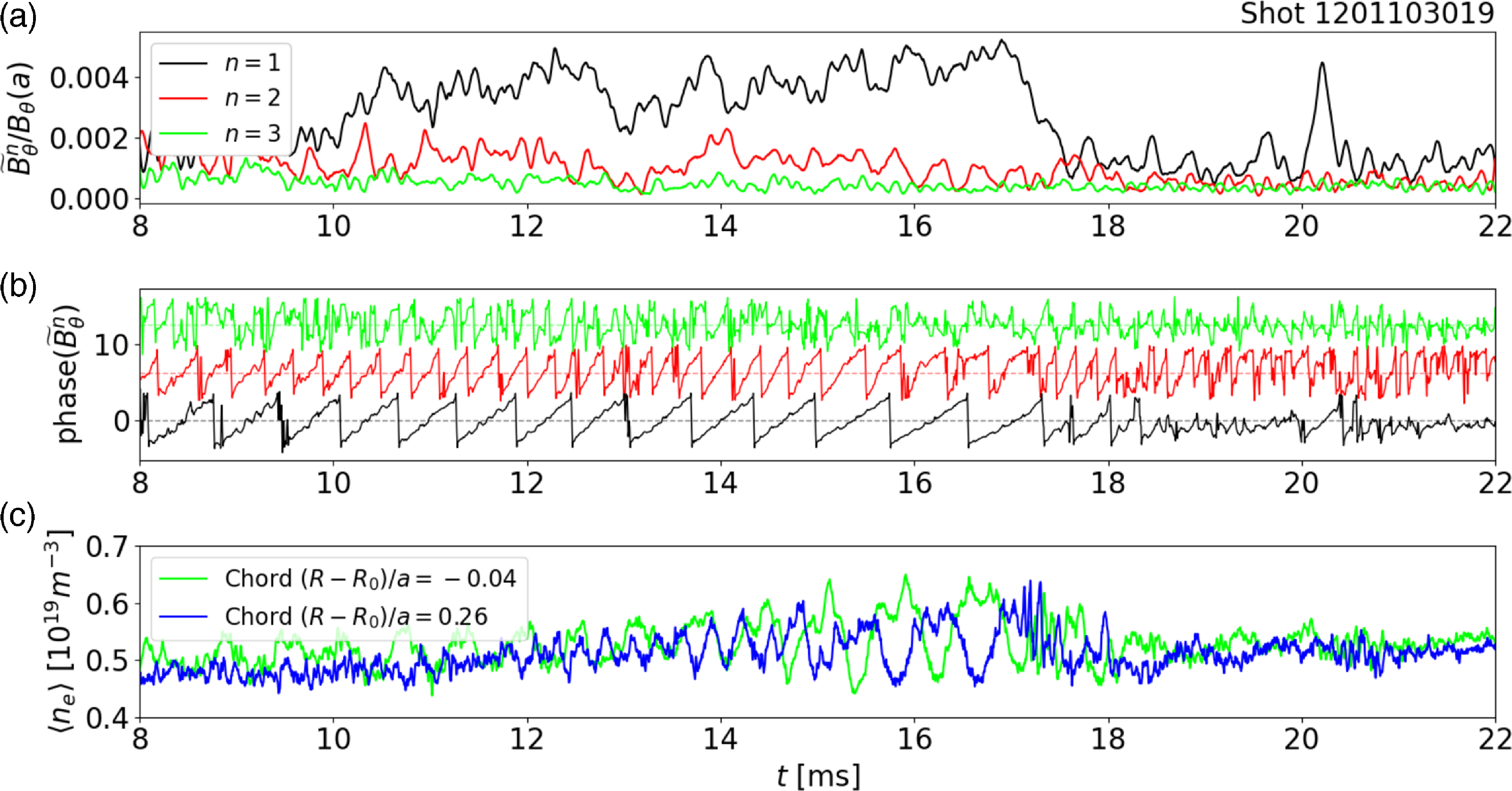
Figure 7. Data from the edge toroidal coil array show (a) magnetic mode amplitudes and (b) phases with $n=1-3$
, which are correlated with the snake density perturbation measured by two interferometer chords shown in panel (c), for the same event shown in figure 1. The rotating
$n=1-3$
, which are correlated with the snake density perturbation measured by two interferometer chords shown in panel (c), for the same event shown in figure 1. The rotating $n=1$
mode is dominant before the snake appears in the interferometer diagnostic, until its termination around
$n=1$
mode is dominant before the snake appears in the interferometer diagnostic, until its termination around $t = 18$
ms. The mode rotates at the same frequency as the density oscillation. Panel (c) shows the off-axis chords nearest to the axis to compare the density snake oscillations with those seen in the magnetics. Here, q(a) = 2.35.
$t = 18$
ms. The mode rotates at the same frequency as the density oscillation. Panel (c) shows the off-axis chords nearest to the axis to compare the density snake oscillations with those seen in the magnetics. Here, q(a) = 2.35.
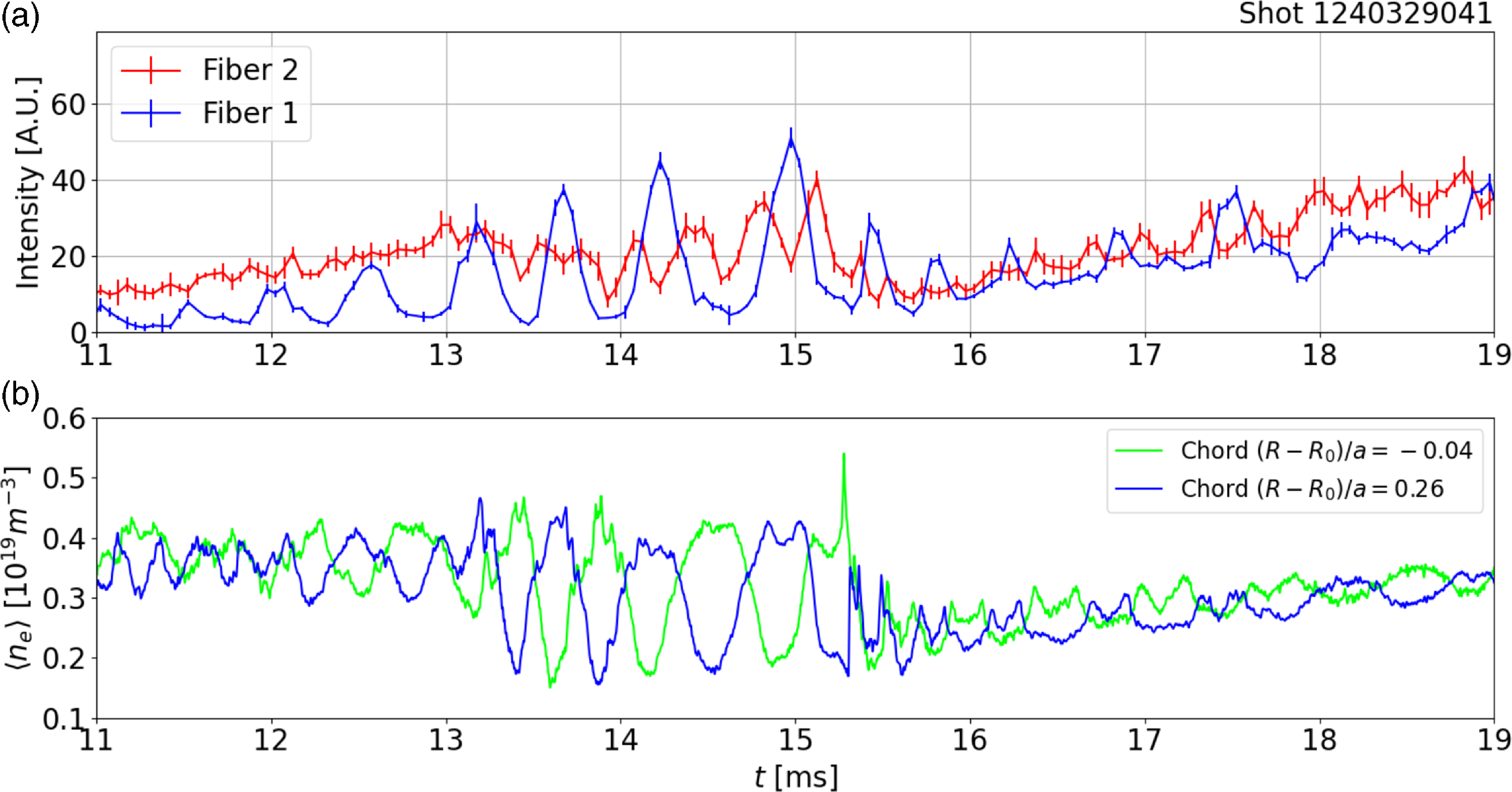
Figure 8. (a) Boron-IV impurity emissions (282 nm) and (b) data from two interferometer chords during a snake event. The fiber 1 line of sight is through the edge of the snake region, whereas fiber 2 is through the magnetic axis. The fiber 1 emission intensity signal was cross-correlated with the density signal to get a phase shift of $32^{\circ }$
, indicating that the intensity oscillations are in phase with the density. Here, q(a) = 2.4.
$32^{\circ }$
, indicating that the intensity oscillations are in phase with the density. Here, q(a) = 2.4.
Impurity emissions of the snake structure have been observed using a high-throughput two-chord spectrometer. Boron IV emission data are shown in figure 8, where the intensity oscillates at the same frequency as the snake. The spectrometer signal in fiber 1, whose viewing chord is tangent to $r/a = 0.45$
, was cross-correlated with the interferometer signal tangent to
$r/a = 0.45$
, was cross-correlated with the interferometer signal tangent to $r/a = 0.42$
, yielding a phase shift of
$r/a = 0.42$
, yielding a phase shift of $32^{\circ }$
. This is near the expected phase shift based on the angular displacements between the two diagnostics,
$32^{\circ }$
. This is near the expected phase shift based on the angular displacements between the two diagnostics, $\Delta \phi = 20^{\circ } + \Delta \theta = 20^\circ + 22^{\circ } = 42^{\circ }$
, where
$\Delta \phi = 20^{\circ } + \Delta \theta = 20^\circ + 22^{\circ } = 42^{\circ }$
, where $\Delta \theta$
is the angle between the two viewing chords. This indicates that the snake volume has a higher B-IV emission intensity compared with the rest of the plasma. If the density is constant, the change in B-IV emissivity is proportional to the boron concentration and nonlinearly increases with electron temperature. Since B-IV was the terminal charge state in this discharge, this relation can be used to infer electron temperature and impurity concentration information since direct measurement was not available. Before
$\Delta \theta$
is the angle between the two viewing chords. This indicates that the snake volume has a higher B-IV emission intensity compared with the rest of the plasma. If the density is constant, the change in B-IV emissivity is proportional to the boron concentration and nonlinearly increases with electron temperature. Since B-IV was the terminal charge state in this discharge, this relation can be used to infer electron temperature and impurity concentration information since direct measurement was not available. Before $t = 13\,\rm ms$
, the density is steady with small oscillations while emission intensities rise gradually. The peaks of the intensity oscillations of fiber 1 coincide with the intensity of fiber 2, suggesting that the snake’s electron temperature and boron concentration are similar to the core’s while the plasma surrounding the snake has one or both values significantly lower. However, since the fiber 1 chord lies at roughly mid-radius, it is unlikely that the temperature inside the snake is higher than the core. This suggests that the intensity difference is due to a greater concentration of boron within the snake. At
$t = 13\,\rm ms$
, the density is steady with small oscillations while emission intensities rise gradually. The peaks of the intensity oscillations of fiber 1 coincide with the intensity of fiber 2, suggesting that the snake’s electron temperature and boron concentration are similar to the core’s while the plasma surrounding the snake has one or both values significantly lower. However, since the fiber 1 chord lies at roughly mid-radius, it is unlikely that the temperature inside the snake is higher than the core. This suggests that the intensity difference is due to a greater concentration of boron within the snake. At $t = 13\,\rm ms$
the core intensity begins to decrease while the snake intensity oscillations grow; at the same time, the large density oscillations begin in both the core and mid-radius chords. Since the fiber 1 chord and snake structure are located at roughly mid-radius, it is unlikely that an increase of the electron temperature within the snake is responsible for the increase in intensity. Since the density oscillations are roughly constant amplitude over
$t = 13\,\rm ms$
the core intensity begins to decrease while the snake intensity oscillations grow; at the same time, the large density oscillations begin in both the core and mid-radius chords. Since the fiber 1 chord and snake structure are located at roughly mid-radius, it is unlikely that an increase of the electron temperature within the snake is responsible for the increase in intensity. Since the density oscillations are roughly constant amplitude over $t = 13\!-\!15\,\rm ms$
, this suggests that the growing intensity oscillation amplitude from the snake is due to an increasing boron concentration in the snake structure. At
$t = 13\!-\!15\,\rm ms$
, this suggests that the growing intensity oscillation amplitude from the snake is due to an increasing boron concentration in the snake structure. At $t = 15\,\rm ms$
, the snake structure dissipates to small density oscillations at a lower average density than during the snake formation, and the emission intensity of both core and snake region fall to similar values. These observations are consistent with models of snake formation based on impurity accumulation.
$t = 15\,\rm ms$
, the snake structure dissipates to small density oscillations at a lower average density than during the snake formation, and the emission intensity of both core and snake region fall to similar values. These observations are consistent with models of snake formation based on impurity accumulation.
3.2. Comparison with ideal and resistive kink models
Based on simple, qualitative models of $m/n = 1/1$
perturbed density profiles described below, we find that the density snakes discussed here are roughly consistent with a saturated resistive kink instability, as opposed to an ideal kink or the crescent-shaped snakes observed on Alcator C-Mod (Delgado-Aparicio et al. Reference Delgado-Aparicio2013
b). The resistive kink features reconnected flux that forms a magnetic island structure surrounding a roughly axisymmetric, higher-density snake core, whereas the ideal kink structure maintains nested flux surfaces. The crescent shape is similar in topology to the quasi-interchange mode that has been proposed as a mechanism for the sawtooth instability (Wesson Reference Wesson2004).
$m/n = 1/1$
perturbed density profiles described below, we find that the density snakes discussed here are roughly consistent with a saturated resistive kink instability, as opposed to an ideal kink or the crescent-shaped snakes observed on Alcator C-Mod (Delgado-Aparicio et al. Reference Delgado-Aparicio2013
b). The resistive kink features reconnected flux that forms a magnetic island structure surrounding a roughly axisymmetric, higher-density snake core, whereas the ideal kink structure maintains nested flux surfaces. The crescent shape is similar in topology to the quasi-interchange mode that has been proposed as a mechanism for the sawtooth instability (Wesson Reference Wesson2004).
We use a simple model for the density profile to create synthetic fluctuations that can be compared with MST measurements. The model parameters allow profiles that are shifted, as for an ideal kink, or have island structure, as for resistive instability. The density is assumed to be a flux function, so the model characterizes distorted flux surfaces. In the resistive case with a magnetic island, the density inside the island is assumed constant, consistent with expected density and temperature flattening due to rapid parallel transport. In the quasi-interchange case, the density is taken to be constant inside the circular region opposite the crescent-shaped, high-density snake core. A simple expression is used to model the displacement of the flux surfaces in the poloidal plane due to the ideal kink motion. The resistive case uses the same model, but includes a simple algorithm to artificially flatten the density in the island. The quasi-interchange case uses a slightly different model, and a flattening algorithm similar to the resistive case. Synthetic interferometer data are generated using these models, and the results are compared with experimental interferometer data for the snake event shown in figure 1. These models are simple and are intended primarily for qualitative comparison; rigorous analytical treatments of kink motion based on the MHD equations are not considered here, but can be found in Biskamp (Reference Biskamp1997).
The toroidally symmetric density distribution in the poloidal plane prior to snake formation is modeled as
 \begin{equation} n_s(\mathbf{r}) = n_0 [1 - (r/a)^2]^b,\end{equation}
where $\mathbf{r} = (r, \theta)$
is a cylindrical coordinate system for which the origin coincides with the magnetic axis
$\mathbf{r} = (r, \theta)$
is a cylindrical coordinate system for which the origin coincides with the magnetic axis $(R = R_0 + \Delta, Z = 0)$
, where
$(R = R_0 + \Delta, Z = 0)$
, where $\Delta$
is the Shafranov shift. Here, the shift
$\Delta$
is the Shafranov shift. Here, the shift $\Delta$
is taken to be constant across the poloidal plane. The error introduced by this simplification is small when comparing the model with the interferometer data, since the signal is dominated by the high-density plasma core at small
$\Delta$
is taken to be constant across the poloidal plane. The error introduced by this simplification is small when comparing the model with the interferometer data, since the signal is dominated by the high-density plasma core at small $r$
where the constant shift is a reasonable approximation. The parameter values
$r$
where the constant shift is a reasonable approximation. The parameter values $n_0 = 0.68 \times 10^{19}$
m
$n_0 = 0.68 \times 10^{19}$
m $^{-3}$
,
$^{-3}$
, $b=3$
and
$b=3$
and $\Delta /a = 0.1$
provide a good fit to the data prior to snake formation (from
$\Delta /a = 0.1$
provide a good fit to the data prior to snake formation (from $t=12-13$
ms in figure 1).
$t=12-13$
ms in figure 1).
The ideal kink is modeled using a coordinate transformation $n_i(\mathbf{r}) \rightarrow n_i(\mathbf{r} - \mathbf{\xi })$
, where
$n_i(\mathbf{r}) \rightarrow n_i(\mathbf{r} - \mathbf{\xi })$
, where $\mathbf{\xi } = \xi _0 \exp [-(r/r_1)^d] [\cos (\phi) {\hat {\mathbf{x}}} + \sin (\phi) {\hat {\mathbf{y}}}]$
is the displacement vector,
$\mathbf{\xi } = \xi _0 \exp [-(r/r_1)^d] [\cos (\phi) {\hat {\mathbf{x}}} + \sin (\phi) {\hat {\mathbf{y}}}]$
is the displacement vector, $\xi _0$
is the displacement amplitude,
$\xi _0$
is the displacement amplitude, $r_1$
is the resonant radius, the exponent
$r_1$
is the resonant radius, the exponent $d=2$
controls the shape of the perturbation,
$d=2$
controls the shape of the perturbation, $\phi$
is the toroidal coordinate and
$\phi$
is the toroidal coordinate and $({\hat {\mathbf{x}}}, {\hat {\mathbf{y}}})$
are unit vectors in a Cartesian coordinate system with the same origin as
$({\hat {\mathbf{x}}}, {\hat {\mathbf{y}}})$
are unit vectors in a Cartesian coordinate system with the same origin as $\mathbf{r}$
. The resistive kink is modeled by
$\mathbf{r}$
. The resistive kink is modeled by $n_r = \mathrm{max}(n_i, n_{{flat}})$
, where
$n_r = \mathrm{max}(n_i, n_{{flat}})$
, where $n_{{flat}}$
is the symmetric density profile given by (3.1) but artificially flattened in the core
$n_{{flat}}$
is the symmetric density profile given by (3.1) but artificially flattened in the core
 \begin{equation} n_{{flat}} = \begin{cases} n_s \ \mathrm{for} \ r \geqslant r_1; \\ n_s(r_1) \ \mathrm{for} \ r \lt r_1. \end{cases} \end{equation}
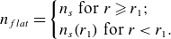
Figure 9. Electron density distributions for models of (a) an ideal kink, (b) a resistive kink and (c) a quasi-interchange mode, with phase $\phi =0$
(see text for details). Profiles of the distributions along
$\phi =0$
(see text for details). Profiles of the distributions along $(R,Z=0)$
are given in panel (d) along with the corresponding symmetric profile.
$(R,Z=0)$
are given in panel (d) along with the corresponding symmetric profile.
This yields a kink structure that is identical to the ideal case but with a flattened crescent region next to the high-density snake core that models the expected flat density distribution inside the magnetic island. For the quasi-interchange case, the crescent shape is generated by taking $d=4$
and a larger value of
$d=4$
and a larger value of $a_1$
. The flattening algorithm increases the density inside the circular region opposite the snake core up to its value at the separatrix.
$a_1$
. The flattening algorithm increases the density inside the circular region opposite the snake core up to its value at the separatrix.
The density distribution from these models are shown in figure 9 for $\phi =0$
, with the ideal case in panel (a), the resistive case in panel (b) and the quasi-interchange case in panel (c). Slices of these distributions along
$\phi =0$
, with the ideal case in panel (a), the resistive case in panel (b) and the quasi-interchange case in panel (c). Slices of these distributions along $(R, Z=0)$
are shown in panel (d) along with the symmetric case.
$(R, Z=0)$
are shown in panel (d) along with the symmetric case.
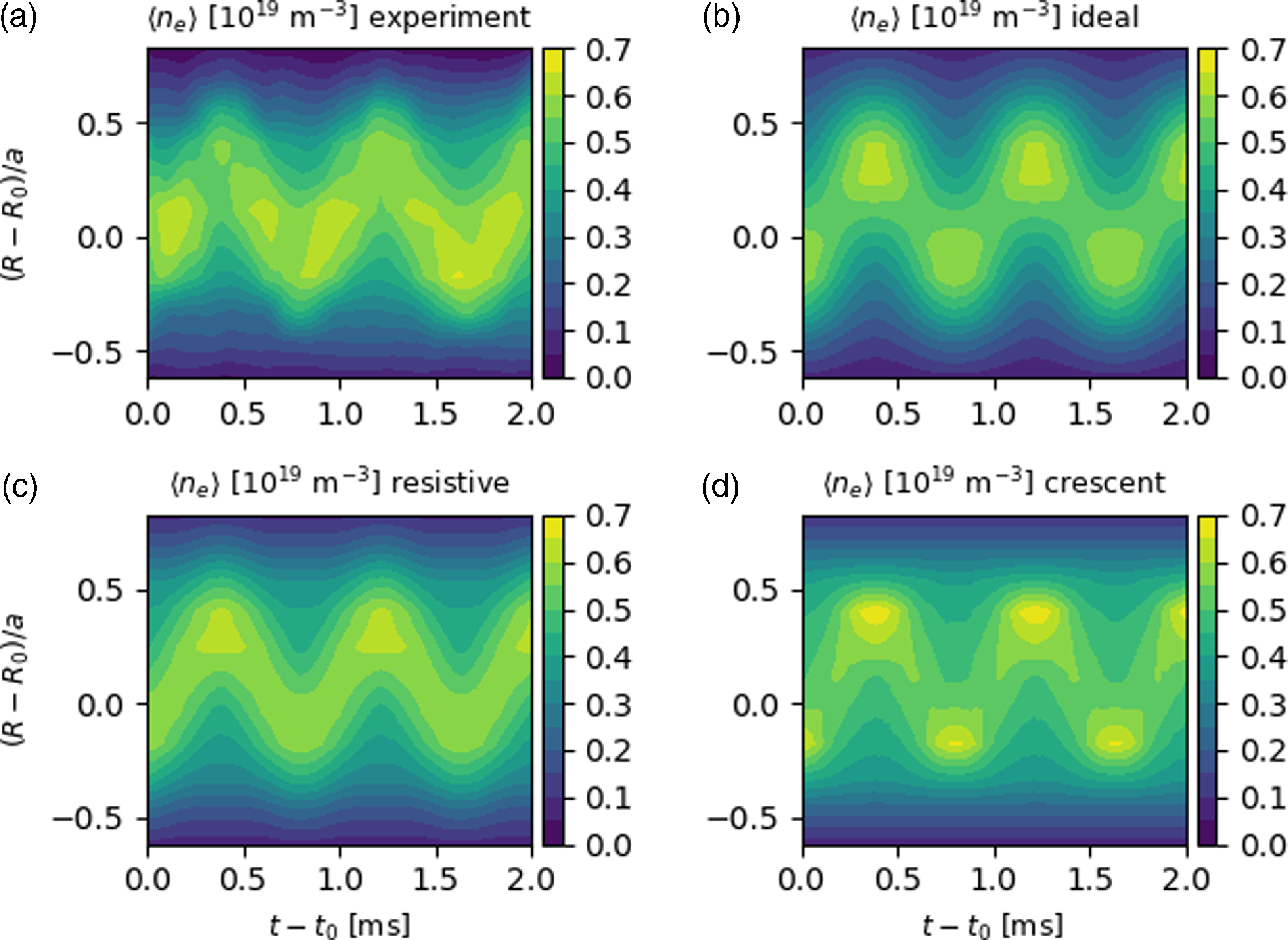
Figure 10. Experimental data of chord-averaged electron density from the 11-chord interferometer are shown in (a) for approximately two periods of the density snake event shown in figure 1. They are compared with synthetic data generated from simple models of (b) an ideal kink, (c) a resistive kink and (d) a crescent kink, where (c) appears to be the best fit.
Two additional parameters are introduced to model the time evolution of the rotating snake: a frequency $f$
and a phase shift
$f$
and a phase shift $\phi _0$
. The density distribution is then given as above, but with the phase of the snake core varying in time as
$\phi _0$
. The density distribution is then given as above, but with the phase of the snake core varying in time as $\phi = 2 \pi f t + \phi _0$
. At each time, the density is integrated along 11 chords with the geometry of the MST interferometer system, in order to generate synthetic data to be compared with the experimental data. A window of experimental data is chosen for the example snake shown in figure 1 for 2 ms (approximately 2 cycles) starting at
$\phi = 2 \pi f t + \phi _0$
. At each time, the density is integrated along 11 chords with the geometry of the MST interferometer system, in order to generate synthetic data to be compared with the experimental data. A window of experimental data is chosen for the example snake shown in figure 1 for 2 ms (approximately 2 cycles) starting at $t_0 = 15\,\rm ms$
. The data are low-pass-filtered with a cutoff at 10 kHz to remove higher-frequency fluctuations not associated with the snake rotation. The tunable parameters in the models are manually fitted to the experimental data. The values
$t_0 = 15\,\rm ms$
. The data are low-pass-filtered with a cutoff at 10 kHz to remove higher-frequency fluctuations not associated with the snake rotation. The tunable parameters in the models are manually fitted to the experimental data. The values $n_0 = 0.68 \times 10^{19}$
m
$n_0 = 0.68 \times 10^{19}$
m $^{-3}$
,
$^{-3}$
, $b=3$
and
$b=3$
and $\Delta /a = 0.1$
corresponding to the symmetric case are used, with the crescent case using
$\Delta /a = 0.1$
corresponding to the symmetric case are used, with the crescent case using $n_0 = 0.8$
to maintain similar particle counts in the core. The value
$n_0 = 0.8$
to maintain similar particle counts in the core. The value $r_1/a = 0.45$
is used for the ideal and resistive cases, based on equilibrium reconstructions using the MSTFit code prior to snake formation, but
$r_1/a = 0.45$
is used for the ideal and resistive cases, based on equilibrium reconstructions using the MSTFit code prior to snake formation, but $r_1/a = 0.35$
is used for the quasi-interchange model to better fit the snake width. The value
$r_1/a = 0.35$
is used for the quasi-interchange model to better fit the snake width. The value $a_1 = 0.35$
is used for the ideal and resistive cases to fit the width of the snake perturbation, and
$a_1 = 0.35$
is used for the ideal and resistive cases to fit the width of the snake perturbation, and $a_1 = 0.6$
is used for the quasi-interchange case in order to generate the crescent-shaped snake core.
$a_1 = 0.6$
is used for the quasi-interchange case in order to generate the crescent-shaped snake core.
The experimental interferometer data are compared with the ideal, resistive and crescent kink synthetic data using these parameters in figure 10. Qualitatively, in the resistive case the signal peak oscillates in the major radial coordinate without changing significantly in amplitude, as expected for a rotating positive density perturbation superposed on a constant background. In contrast, for the ideal case the signal is stronger at two phases during the snake period when the high-density core is located either inboard or outboard $\phi = 0, \pi$
. This is because for these phases the interferometer chords passing near the snake core detect only the high-density peak, whereas for the phases
$\phi = 0, \pi$
. This is because for these phases the interferometer chords passing near the snake core detect only the high-density peak, whereas for the phases $\phi = \pi /2, 3 \pi /2$
the central chords integrate over both the positive and negative parts of the perturbation. For the quasi-interchange (crescent) case, higher-signal regions appear at phases
$\phi = \pi /2, 3 \pi /2$
the central chords integrate over both the positive and negative parts of the perturbation. For the quasi-interchange (crescent) case, higher-signal regions appear at phases $\phi = 0, \pi$
similar to the ideal kink case, but more pronounced. This is because at these phases the elongated direction of the crescent is aligned with the interferometer chord, thus increasing the integrated signal relative to the phases
$\phi = 0, \pi$
similar to the ideal kink case, but more pronounced. This is because at these phases the elongated direction of the crescent is aligned with the interferometer chord, thus increasing the integrated signal relative to the phases $\phi = \pi /2, 3 \pi /2$
.
$\phi = \pi /2, 3 \pi /2$
.
The experimental signal is not significantly enhanced on the inboard or outboard side, and therefore appears to be most qualitatively consistent with the resistive kink model. The 2-D arrays of modeled interferometer data are subtracted from the experimental one, and the mean of the absolute value of the difference is calculated, yielding an average error of 0.048 for the ideal case, 0.041 for the resistive case and 0.053 for the quasi-interchange case. Thus, the resistive model appears to be the best fit quantitatively, although not by a large margin. These results are based on simple, qualitative models, and should be interpreted with caution. More rigorous modeling efforts are outside the scope of this paper, but will be performed in the future to seek firmer conclusions. The interpretation of the snakes as resistive kink structures is consistent with the relatively low Lundquist number, $S \sim 10^5$
, in MST tokamak plasmas relative to other modern tokamaks. Additionally, theoretical analysis has shown that the internal kink saturates at relatively low amplitude (Biskamp Reference Biskamp1997), so resistive behavior can be expected for the relatively large snakes studied here. Interestingly, the snakes discussed here appear to be more consistent with resistive kink behavior than with quasi-interchange behavior featuring crescent-shaped snake cores, such as that observed in Alcator C-Mod (Delgado-Aparicio et al. Reference Delgado-Aparicio2013
b). This might be attributed to the lack of auxiliary heating and lower pressure in MST, such that the current gradient is more important than the pressure gradient in driving the instability.
$S \sim 10^5$
, in MST tokamak plasmas relative to other modern tokamaks. Additionally, theoretical analysis has shown that the internal kink saturates at relatively low amplitude (Biskamp Reference Biskamp1997), so resistive behavior can be expected for the relatively large snakes studied here. Interestingly, the snakes discussed here appear to be more consistent with resistive kink behavior than with quasi-interchange behavior featuring crescent-shaped snake cores, such as that observed in Alcator C-Mod (Delgado-Aparicio et al. Reference Delgado-Aparicio2013
b). This might be attributed to the lack of auxiliary heating and lower pressure in MST, such that the current gradient is more important than the pressure gradient in driving the instability.
3.3. Growth, decay and transient behavior
Density snakes typically form spontaneously within tokamak discharges after the initial set up phase, when diffusive current peaking has proceeded such that $q(0)$
approaches unity. Pellet fueling was not used in these studies, and the impurity emission data do not accurately predict the onset of a snake. Based on a review of snake events, we find that snakes tend to form when the density profile is highly peaked during startup, but not in a repeatable manner (i.e. not in every shot). This formation first begins as small magnetic oscillations prior to any major density perturbation, as shown in figure 7. Following this, small density perturbations are observed, particularly in the outboard contour of figure 4. These perturbations in both the magnetic and density signals slowly grow in space and magnitude until the snake reaches a quasi-steady state.
$q(0)$
approaches unity. Pellet fueling was not used in these studies, and the impurity emission data do not accurately predict the onset of a snake. Based on a review of snake events, we find that snakes tend to form when the density profile is highly peaked during startup, but not in a repeatable manner (i.e. not in every shot). This formation first begins as small magnetic oscillations prior to any major density perturbation, as shown in figure 7. Following this, small density perturbations are observed, particularly in the outboard contour of figure 4. These perturbations in both the magnetic and density signals slowly grow in space and magnitude until the snake reaches a quasi-steady state.
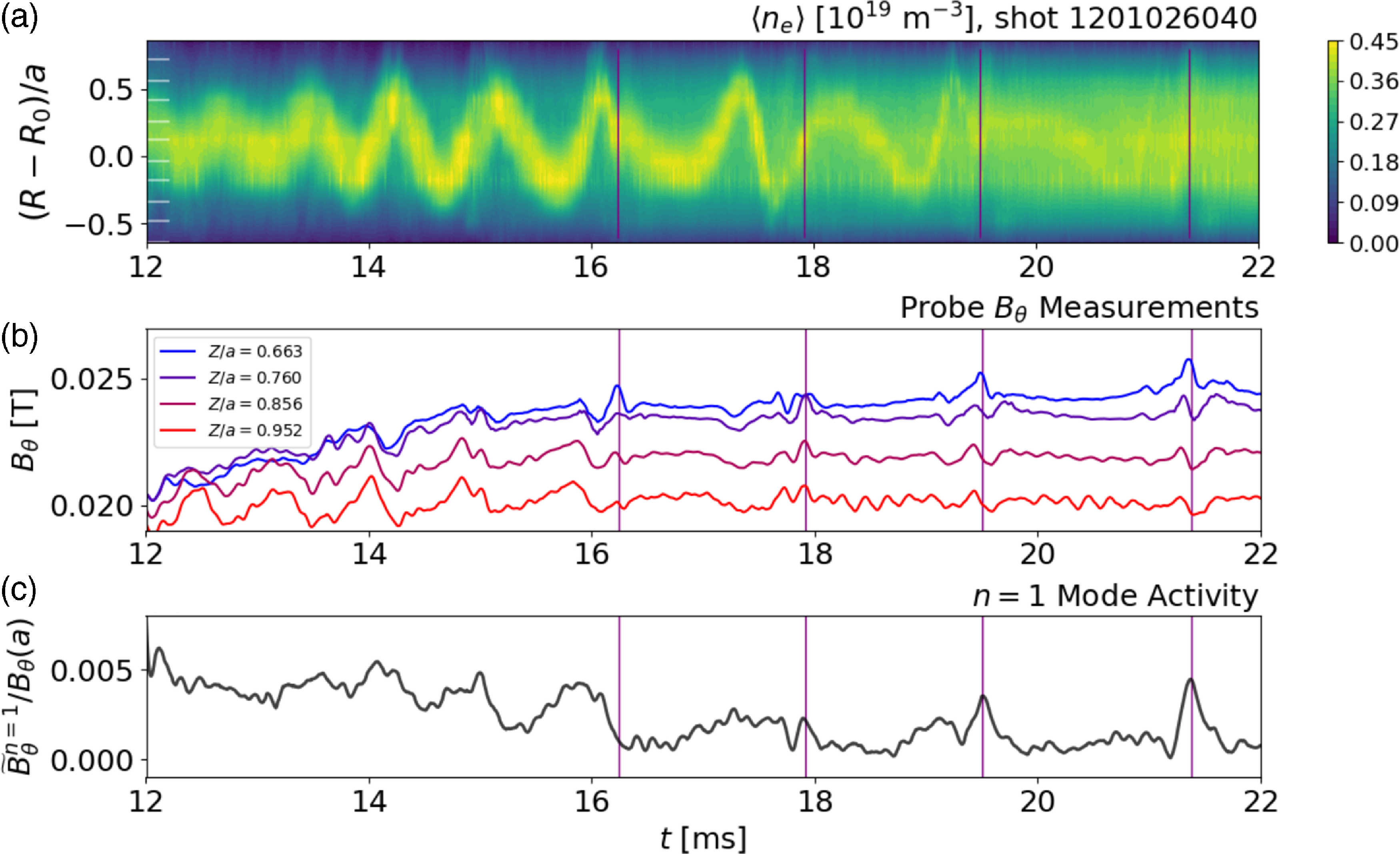
Figure 11. Perturbation of a density snake due to sawtooth crashes. (a) Interferometer data showing the snake structure, (b) deep-insertion probe signals and (c) the normalized amplitude of the $n=1$
poloidal field perturbation measured by the edge magnetic array. The crash times are identified as burst of activity in the magnetic signals, and are indicated as vertical purple lines. Each crash significantly perturbs the snake rotation frequency, radial size and density perturbation, until it gradually disappears. Here, q(a) = 2.27.
$n=1$
poloidal field perturbation measured by the edge magnetic array. The crash times are identified as burst of activity in the magnetic signals, and are indicated as vertical purple lines. Each crash significantly perturbs the snake rotation frequency, radial size and density perturbation, until it gradually disappears. Here, q(a) = 2.27.
During this stable period, however, amplitude and frequency changes are sometimes observed. The radial size of the snake will slowly grow until saturation, with the frequency remaining constant. After some time, the sawtooth cycle begins. There are two outcomes to the snake interacting with sawtooth crashes. Most often, the snake terminates at the first major crash, as observed in figure 1. Fast, turbulent activity is seen at $t = 17\,\rm ms$
, aligning with strong magnetic activity attributed to the sawtooth crash in MST. The other, less common outcome is severe perturbation of the snake. Figure 11 shows a snake surviving multiple sawtooth crashes in a plasma with
$t = 17\,\rm ms$
, aligning with strong magnetic activity attributed to the sawtooth crash in MST. The other, less common outcome is severe perturbation of the snake. Figure 11 shows a snake surviving multiple sawtooth crashes in a plasma with $q(a) = 2.2$
. After the first crash, the rotation frequency and radial amplitude both decrease, slowly stabilizing again, only to encounter another sawtooth crash. If the sawtooth cycle is slower, the snake can return to another stable state with a different radial amplitude and rotation frequency before encountering another sawtooth event which either terminates or perturbs the snake again. At higher values of
$q(a) = 2.2$
. After the first crash, the rotation frequency and radial amplitude both decrease, slowly stabilizing again, only to encounter another sawtooth crash. If the sawtooth cycle is slower, the snake can return to another stable state with a different radial amplitude and rotation frequency before encountering another sawtooth event which either terminates or perturbs the snake again. At higher values of $q(a)$
, snakes are more frequently observed which last through several sawtooth crashes, but more data are needed to understand this trend in detail.
$q(a)$
, snakes are more frequently observed which last through several sawtooth crashes, but more data are needed to understand this trend in detail.
Following termination of a snake, the plasma density profile broadens compared with before its formation. The density perturbation associated with the snake dissipates while the equilibrium profile broadens, indicating outward radial transport through the sawtooth crash. Toroidal equilibrium reconstructions using the MSTFit code (Anderson et al. Reference Anderson, Forest, Biewer, Sarff and Wright2004) were done before and after the snake to confirm this. The resulting radial density profiles are shown in figure 12. After the snake dissipates, the plasma is comparable to discharges which have no snake to begin with.
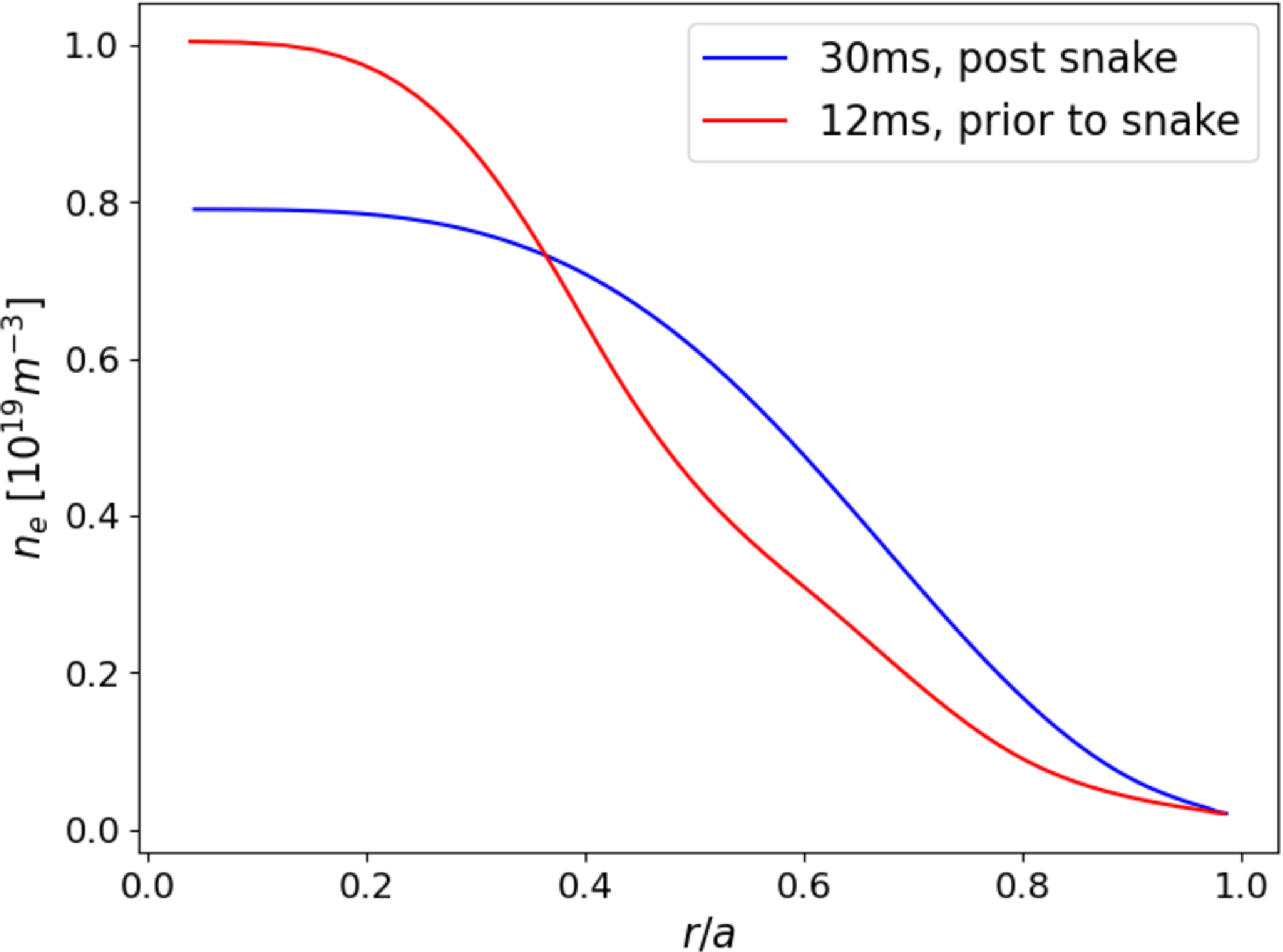
Figure 12. Density profiles calculated from toroidal equilibrium reconstructions using the MSTFit code. Shown are two profiles from the same discharge, before and after a density snake occurs. The profile change indicates a radial transport of density after the density snake dissipates. Here, q(a) = 2.07.
4. Discussion
There are still many outstanding questions about the formation, structure and termination of helical density snake structures in tokamaks. Of particular interest is the interaction between the density snake and the sawtooth crash, both of which are associated with internal kink modes of helicity $m/n = 1/1$
. In other experiments these interactions typically cause small perturbations to the snake structure, whereas in the experiments presented here the snakes are often strongly perturbed or terminated. One possible reason for this is that the MST tokamak discharges are often run in a lower range of edge safety factor compared with other machines, which is thought to result in broader, more unstable helical structures.
$m/n = 1/1$
. In other experiments these interactions typically cause small perturbations to the snake structure, whereas in the experiments presented here the snakes are often strongly perturbed or terminated. One possible reason for this is that the MST tokamak discharges are often run in a lower range of edge safety factor compared with other machines, which is thought to result in broader, more unstable helical structures.
Another consideration is the lower toroidal field, plasma current and temperature of the MST tokamak plasmas relative to other modern, high-performance tokamak experiments, which is also likely to impact many aspects of snake dynamics and stability. In particular, resistive effects such as magnetic reconnection and the formation of magnetic islands is more likely.
The lack of resiliency of density snakes observed in MST tokamak plasmas is consistent with predictions by Sugiyama (Reference Sugiyama2013) in the case of large radius of the $q=1$
rational surface,
$q=1$
rational surface, $r_1$
, where the high-density and temperature regions are supposed to align. This would cause the hot, sawtoothing core to deposit the snake density outside of the core, leading to the termination of the snake. Whether the density and temperature are aligned for snakes in MST is still unknown, yet the decreased resiliency hints towards that conclusion. While impurity ion spectrometer data are lacking for the high
$r_1$
, where the high-density and temperature regions are supposed to align. This would cause the hot, sawtoothing core to deposit the snake density outside of the core, leading to the termination of the snake. Whether the density and temperature are aligned for snakes in MST is still unknown, yet the decreased resiliency hints towards that conclusion. While impurity ion spectrometer data are lacking for the high $q(a)$
discharges produced for this study, there may be clues within that region of parameter space where snakes are more likely to survive through the sawtooth crash. If both resilient and fragile snakes can be produced in MST, it may be possible to study whether there is a smooth transition between the two cases as opposed to a sharp change in snake resiliency.
$q(a)$
discharges produced for this study, there may be clues within that region of parameter space where snakes are more likely to survive through the sawtooth crash. If both resilient and fragile snakes can be produced in MST, it may be possible to study whether there is a smooth transition between the two cases as opposed to a sharp change in snake resiliency.
Another important question regards whether the snake is best described as an ideal internal kink mode with $m/n = 1/1$
or a resistive one featuring a magnetic island. The internal structure of snakes in Alcator C-mod have been well characterized by Delgado-Aparicio et al. (Reference Delgado-Aparicio2013
b) using a full suite of diagnostic cameras, revealing both types of mode (ideal and resistive) at different stages of the snake life cycle. This type of measurement is unavailable in MST at present due to the low electron temperature. The simple model presented in § 3.2 suggests that the snake structure more closely resembles that of a resistive kink featuring a large island with flattened density, compared with an ideal kink or a crescent-shaped snake core observed in Alcator C-Mod.
$m/n = 1/1$
or a resistive one featuring a magnetic island. The internal structure of snakes in Alcator C-mod have been well characterized by Delgado-Aparicio et al. (Reference Delgado-Aparicio2013
b) using a full suite of diagnostic cameras, revealing both types of mode (ideal and resistive) at different stages of the snake life cycle. This type of measurement is unavailable in MST at present due to the low electron temperature. The simple model presented in § 3.2 suggests that the snake structure more closely resembles that of a resistive kink featuring a large island with flattened density, compared with an ideal kink or a crescent-shaped snake core observed in Alcator C-Mod.
5. Conclusions
Helical density snake structures associated with internal kink modes with $m=1$
and
$m=1$
and $n=1$
have been studied within MST tokamak plasmas. These snakes exhibit fascinating characteristics throughout their life cycle, which involves formation and growth, saturation, perturbations and eventual termination. They are primarily diagnosed using an 11-chord interferometer diagnostic that yields detailed information about the structure and dynamics of the modes. Measurements from several other diagnostics, including edge and internal magnetic probes and impurity ion spectroscopy, are consistent with the interferometer data for a
$n=1$
have been studied within MST tokamak plasmas. These snakes exhibit fascinating characteristics throughout their life cycle, which involves formation and growth, saturation, perturbations and eventual termination. They are primarily diagnosed using an 11-chord interferometer diagnostic that yields detailed information about the structure and dynamics of the modes. Measurements from several other diagnostics, including edge and internal magnetic probes and impurity ion spectroscopy, are consistent with the interferometer data for a $m/n = 1/1$
structure rotating toroidally at approximately 1.5 kHz, and provide further insight into the mode growth, saturation and dynamics. The snakes observed in MST differ from those reported in other devices, particularly with regard to their formation, resiliency and interaction with the sawtooth cycle. The edge safety factor studied here ranges down to
$m/n = 1/1$
structure rotating toroidally at approximately 1.5 kHz, and provide further insight into the mode growth, saturation and dynamics. The snakes observed in MST differ from those reported in other devices, particularly with regard to their formation, resiliency and interaction with the sawtooth cycle. The edge safety factor studied here ranges down to $q(a) = 2.2$
, significantly lower than most tokamak experiments. This is thought to broaden the radial location of the
$q(a) = 2.2$
, significantly lower than most tokamak experiments. This is thought to broaden the radial location of the $q=1$
resonant surface, causing larger, more unstable snakes that are often terminated at the first sawtooth crash of the discharge. Further experiments in MST with higher
$q=1$
resonant surface, causing larger, more unstable snakes that are often terminated at the first sawtooth crash of the discharge. Further experiments in MST with higher $q(a)$
up to 3.2 show snakes with smaller radial size and greater resiliency, often surviving through multiple crashes. Whereas prior experiments in other devices showed small perturbations to snake parameters (size, rotation frequency, etc.) due to interaction with sawtooth crashes, in MST when a snake survives a crash it is often strongly perturbed. The relatively high resistivity of MST tokamak plasmas likely contributes to the change in snake structure and dynamics compared with other devices. Preliminary modeling suggests that the snakes are best described as saturated resistive kink instabilities featuring large magnetic islands. These results contribute to a broader body of knowledge on the spontaneous bifurcation of axisymmetric toroidal plasmas into 3-D, non-axisymmetric equilibria.
$q(a)$
up to 3.2 show snakes with smaller radial size and greater resiliency, often surviving through multiple crashes. Whereas prior experiments in other devices showed small perturbations to snake parameters (size, rotation frequency, etc.) due to interaction with sawtooth crashes, in MST when a snake survives a crash it is often strongly perturbed. The relatively high resistivity of MST tokamak plasmas likely contributes to the change in snake structure and dynamics compared with other devices. Preliminary modeling suggests that the snakes are best described as saturated resistive kink instabilities featuring large magnetic islands. These results contribute to a broader body of knowledge on the spontaneous bifurcation of axisymmetric toroidal plasmas into 3-D, non-axisymmetric equilibria.
Future work will seek to gather more information about the snake internal structure, including temperature measurements and further magnetic data that could better characterize the snake growth and saturation mechanisms. In particular, experiments in which impurities are injected intentionally could explore the formation mechanism and possibly allow for more repeatable snake production. With sufficient experimental constraints, it may be possible to carry out 3-D helical equilibrium reconstructions using methods developed to study stellarator plasmas. Improved modeling such as this could offer firmer conclusions regarding the resistive kink nature of the snakes. Of particular interest is the stability and robustness of the snakes, including their interaction with other modes such as the sawtooth crash which carries the same helicity, $m/n = 1/1$
. This involves strong nonlinearity and mode coupling which may be difficult to characterize and model, but is essential for understanding the behavior of density snakes in tokamak plasmas.
$m/n = 1/1$
. This involves strong nonlinearity and mode coupling which may be difficult to characterize and model, but is essential for understanding the behavior of density snakes in tokamak plasmas.
Acknowledgements
Editor Cary Forest thanks the referees for their advice in evaluating this article.
Funding
This work was conducted at the Wisconsin Plasma Physics Laboratory (WiPPL), a research facility supported by the DOE Office of Fusion Energy Sciences under contract DE-SC0018266 with major facility instrumentation developed with support from the National Science Foundation under award PHY 1828159.
Declaration of interests
The authors report no conflict of interest.
Data availability
The data that support the findings of this study are available from the corresponding author upon reasonable request.


 Open access