


1 Introduction
The turbulent plasma dynamics in the edge plays a key role in determining the overall performances of a tokamak by governing its confinement properties. Indeed, fundamental phenomena, such as the L–H transition (Wagner et al. Reference Wagner, Becker, Behringer, Campbell, Eberhagen, Engelhardt, Fussmann, Gehre, Gernhardt and Gierke1982) and the density limit (Greenwald et al. Reference Greenwald, Terry, Wolfe, Ejima, Bell, Kaye and Neilson1988; Greenwald Reference Greenwald2002), strongly depend on the plasma dynamics in the tokamak edge. Because of the persisting uncertainties in the fundamental understanding of these phenomena, the design of future fusion devices is based on scaling laws.
A scaling law for the power threshold for the L–H transition,  $P_{\text {LH}}$, has been proposed by Martin, Takizuka & the ITPA CDBM H-mode Threshold Database Working Group (Reference Martin and Takizuka2008) based on an international H-mode threshold power database:
 \begin{equation} P_{\text{{LH}}} \propto n_e^{0.78\pm 0.04} B_T^{0.77\pm 0.03}a^{0.98\pm 0.08}R^{1.0\pm 0.1}, \end{equation}
where  $n_e$ is the line-averaged electron density, $B_T$ is the toroidal magnetic field at the tokamak axis, $a$ is the tokamak minor radius and $R$ is the tokamak major radius. In addition, it has been experimentally observed that $P_{\text {LH}}$ in a single-null geometry is lower when the ion- $\boldsymbol {\nabla } B$ drift direction is towards the X-point, rather than away from it (ASDEX Team 1989) and that $P_{\text {LH}}$ depends inversely on $m_i/m_e$ (Righi et al. Reference Righi, Bartlett, Christiansen, Conway, Cordey, Eriksson, De Esch, Fishpool, Gowers and De Haas1999; Maggi et al. Reference Maggi, Weisen, Hillesheim, Chankin, Delabie, Horvath, Auriemma, Carvalho, Corrigan and Flanagan2017). Experimental observations in Alcator C-Mod (Snipes et al. Reference Snipes, Boivin, Christensen, Fiore, Garnier, Goetz, Golovato, Graf, Granetz and Greenwald1996) and DIII-D (Thomas et al. Reference Thomas, Groebner, Burrell, Osborne and Carlstrom1998) tokamaks have pointed out the presence of hysteresis in the L–H transition, although this is not a feature universally observed (Ryter et al. Reference Ryter, Rathgeber, Orte, Bernert, Conway, Fischer, Happel, Kurzan, McDermott and Scarabosio2013). Furthermore, just before the L–H transition, experimentally observed is the formation at the tokamak edge of a clear well in the radial electric field profile that induces a strong $\boldsymbol {E}\times \boldsymbol {B}$ shear flow, which, in turn, suppresses plasma turbulence (Groebner, Burrell & Seraydarian Reference Groebner, Burrell and Seraydarian1990; Burrell Reference Burrell1997; Ryter et al. Reference Ryter, Cavedon, Happel, McDermott, Viezzer, Conway, Fischer, Kurzan, Pütterich and Tardini2015). While several models have attempted to uncover the mechanism behind the L–H transition, there is no theory that accounts for all the observations (Connor & Wilson Reference Connor and Wilson2000).
The density limit represents the maximum plasma density achievable in tokamaks before the plasma develops a strong magnetohydrodynamic activity that leads to the degradation of particle confinement or even a disruption. An experimental scaling law for the density limit, denoted as Greenwald density  $n_\textrm {G}$, has been derived by Greenwald et al. (Reference Greenwald, Terry, Wolfe, Ejima, Bell, Kaye and Neilson1988):
 \begin{equation} n_\textrm{G} = \frac{I_p}{{\rm \pi} a^2}, \end{equation}
where  $I_p$ is the plasma current in MA, $a$ is the tokamak minor radius in m and $n_\textrm {G}$ is the line-averaged density in $10^{20}\ \textrm {m}^{-3}$. Experimental observations show that the cooling of the plasma edge is a key element that characterizes the density limit (Vershkov & Mirnov Reference Vershkov and Mirnov1974; Fielding et al. Reference Fielding, Hugill, McCracken, Paul, Prentice and Stott1977). In fact, experimental studies reveal that the density limit can be exceeded by operating with peaked density profiles (Kamada et al. Reference Kamada, Hosogane, Yoshino, Hirayama and Tsunematsu1991; Mahdavi et al. Reference Mahdavi, Osborne, Leonard, Chu, Doyle, Fenstermacher, McKee, Staebler, Petrie and Wade2002; Valovic et al. Reference Valovic, Rapp, Cordey, Budny, McDonald, Garzotti, Kallenbach, Mahdavi, Ongena and Parail2002; Lang et al. Reference Lang, Suttrop, Belonohy, Bernert, Mc Dermott, Fischer, Hobirk, Kardaun, Kocsis and Kurzan2012), thus providing a strong evidence of the link between the density limit and edge physics (Greenwald Reference Greenwald2002). It has been experimentally observed by Hong et al. (Reference Hong, Tynan, Diamond, Nie, Guo, Long, Ke, Wu, Yuan and Xu2017) that, when the line-averaged density approaches the density limit, the edge shear flow collapses and, consequently, the turbulent transport strongly increases near the separatrix. While there is no widely accepted first-principles model for the density limit, research in this area has focused on mechanisms which lead to strong edge cooling, in particular on the effect of the plasma collisionality on enhanced turbulent transport (Greenwald Reference Greenwald2002).
The first attempts to provide a unified theoretical description of turbulent transport in the tokamak edge that includes the L-mode confinement regime, the H-mode confinement regime and a degraded confinement regime, related to the crossing of the density limit, are discussed by Scott (Reference Scott1997) and Rogers, Drake & Zeiler (Reference Rogers, Drake and Zeiler1998) in a circular and sheared geometry, based on fluid flux-tube simulations. The transitions from the L-mode to the H-mode and from the L-mode to the density limit are observed by changing the value of the plasma collisionality and  $\beta$. The dependence of edge transport on these parameters was then experimentally observed by LaBombard et al. (Reference LaBombard, Hughes, Mossessian, Greenwald, Lipschultz and Terry2005). A more recent work (Hajjar, Diamond & Malkov Reference Hajjar, Diamond and Malkov2018) based on the Hasegawa–Wakatani model (Hasegawa & Wakatani Reference Hasegawa and Wakatani1983) in the low- $\beta$ limit shows that both the dynamics that characterizes the L–H transition and the density limit can be described as the result of varying the plasma collisionality. By changing the collisionality, three different regimes are identified: a low-confinement regime, a high-confinement regime and a regime of degraded particle confinement, which is associated with the density limit.
The goal of the present paper is to extend previous investigations of the edge turbulent regimes by considering a more realistic geometry, i.e. a lower single-null configuration, while retaining the coupling between the edge and both the core and the scrape-off layer (SOL), as a crucial element in determining the plasma dynamics at the tokamak edge. In fact, the transport mechanisms occurring in the tokamak periphery are expected to result from a complex interplay among core, edge and SOL physics (Fichtmüller, Corrigan & Simonini Reference Fichtmüller, Corrigan and Simonini1998; Dif-pradalier et al. Reference Dif-pradalier, Caschera, Ghendrih, Donnel, Garbet, Grandgirard, Latu, Norscini and Sarazin2017; Grenfell et al. Reference Grenfell, van Milligen, Losada, Estrada, Liu, Silva, Spolaore and Hidalgo2019), which is difficult to properly model with a simulation domain that does not include all of them. As a consequence, we perform turbulence simulations of the whole tokamak in order to approach this interplay.
Turbulence in the tokamak core is most often simulated by means of gyrokinetic codes, while fluid codes are usually applied in the SOL, taking advantage of its higher plasma collisionality. This separation undermines the possibilities to advance our understanding of the plasma dynamics in the tokamak edge. For this reason, recently, significant effort has been made in order to extend gyrokinetic models towards the edge and the SOL (Qin et al. Reference Qin, Cohen, Nevins and Xu2007; Hahm, Wang & Madsen Reference Hahm, Wang and Madsen2009; Frei, Jorge & Ricci Reference Frei, Jorge and Ricci2020). The first gyrokinetic simulation of the L–H transition that encompasses the edge and the SOL was carried out using the XGC1 code (Chang et al. Reference Chang, Ku, Tynan, Hager, Churchill, Cziegler, Greenwald, Hubbard and Hughes2017; Ku et al. Reference Ku, Chang, Hager, Churchill, Tynan, Cziegler, Greenwald, Hughes, Parker and Adams2018). Since the computational cost of a gyrokinetic simulation of the L–H transition on a global transport time scale remains prohibitively high (Chang et al. Reference Chang, Ku, Tynan, Hager, Churchill, Cziegler, Greenwald, Hubbard and Hughes2017), an ion heat flux at the edge was imposed in the XGC1 L–H simulation, considerably larger than the experimental one. This large flux allowed a reduced computational cost of the simulation, as the L–H transition was due to fast electrostatic bifurcation occurring on a time scale considerably shorter than the one required to reach the global steady-state transport conditions. Other efforts to extend gyrokinetic codes to simulate turbulence in open-field-line systems include the Gkeyll (Shi et al. Reference Shi, Hammett, Stoltzfus-Dueck and Hakim2017), GENE (Pan et al. Reference Pan, Told, Shi, Hammett and Jenko2018), ELMFIRE (Chôné et al. Reference Chôné, Kiviniemi, Leerink, Niskala and Rochford2018) and COGENT (Dorf & Dorr Reference Dorf and Dorr2020) codes. In this paper, we follow a different approach and we extend fluid simulations to the core region, in order to cover the whole tokamak plasma volume. While not providing an accurate description of turbulence in the core, these simulations allow us to explore the parameter space of edge turbulence at different values of heat source and plasma collisionality in a global transport steady state that is the result of the heat and particle sources in the core, turbulent transport and the losses at the vessel. Using these simulations, we draw a portrait of the edge turbulent regimes that can be used as a basis to interpret the results of more complete kinetic simulations.
Our study is based on simulations carried out with GBS (Ricci et al. Reference Ricci, Halpern, Jolliet, Loizu, Mosetto, Fasoli, Furno and Theiler2012; Halpern et al. Reference Halpern, Ricci, Jolliet, Loizu, Morales, Mosetto, Musil, Riva, Tran and Wersal2016; Paruta et al. Reference Paruta, Ricci, Riva, Wersal, Beadle and Frei2018), a three-dimensional, flux-driven, two-fluid simulation code that has been developed to study plasma turbulence in the tokamak boundary. Similarly to other turbulent codes, such as BOUT++ (Dudson et al. Reference Dudson, Allen, Breyiannis, Brugger, Buchanan, Easy, Farley, Joseph, Kim and McGann2015), GDB (Zhu, Francisquez & Rogers Reference Zhu, Francisquez and Rogers2018), GRILLIX (Stegmeir et al. Reference Stegmeir, Coster, Ross, Maj, Lackner and Poli2018), HESEL (Nielsen et al. Reference Nielsen, Xu, Madsen, Naulin, Juul Rasmussen and Wan2015) and TOKAM3X (Tamain et al. Reference Tamain, Bufferand, Ciraolo, Colin, Galassi, Ghendrih, Schwander and Serre2016), GBS evolves the drift-reduced Braginskii's equations (Zeiler, Drake & Rogers Reference Zeiler, Drake and Rogers1997), a set of two-fluid equations valid for describing phenomena occurring on time scales longer than  $1/\varOmega _{ci}$, with $\varOmega _{ci}=eB_T/m_i$ the ion cyclotron frequency, perpendicular length scales longer than the ion Larmor radius and parallel length scales longer than the mean free path.
Early fluid simulations performed with the BOUT code have already shown that the physics of the L–H transition can be addressed by means of fluid models (Xu et al. Reference Xu, Cohen, Rognlien and Myra2000, Reference Xu, Cohen, Nevins, Porter, Rensink, Rognlien, Myra, D'Ippolito, Moyer and Snyder2002), even though fluid models exclude a large fraction of modes that are relevant to edge transport, e.g. trapped electron modes, electron temperature gradients, microtearing modes and kinetic ballooning modes, while retaining the fluid limit of the ion temperature gradient modes (Mosetto et al. Reference Mosetto, Halpern, Jolliet, Loizu and Ricci2015). Later numerical investigations of the L–H transition have been carried out using two- and three-dimensional fluid simulations and have pointed out the spontaneous formation of a transport barrier (Rasmussen et al. Reference Rasmussen, Nielsen, Madsen, Naulin and Xu2015; Chôné et al. Reference Chôné, Beyer, Sarazin, Fuhr, Bourdelle and Benkadda2014, Reference Chôné, Beyer, Sarazin, Fuhr, Bourdelle and Benkadda2015). Indeed, despite their simplicity, our simulations show the presence of three turbulent transport regimes: (i) a developed transport regime, which we associate with the standard L-mode; (ii) a suppressed transport regime, characterized by a higher value of the energy confinement time due to the onset of a transport barrier near the separatrix, and a lower relative fluctuation level, with features that recall the H-mode; and (iii) a degraded confinement regime, characterized by a catastrophically large turbulent transport, which we link to the density limit. In the developed transport regime and degraded confinement regime, turbulent transport is driven by the interchange instability, while in the suppressed transport regime it is driven by the Kelvin–Helmholtz (KH) instability. We then analyse the transitions between these regimes. As the heat source increases, a transition from the developed transport regime to the suppressed transport regime is observed. This transition is due to the formation of a strong  $\boldsymbol {E}\times \boldsymbol {B}$ shear across the separatrix, which stabilizes the interchange instability and destabilizes the KH instability. At the transition, a transport barrier forms at the tokamak edge and, consequently, the energy confinement time increases by a factor of approximately two. In fact, the transition from the developed transport regime to the suppressed transport regime shows common features to the L–H transition observed in experiments. By imposing a flux balance at the separatrix between perpendicular and parallel transport, we then derive an equation for the heat source threshold, which can be identified as the power threshold for H-mode access, that we compare to the experimental scaling law of (1.1). The transition from the developed transport regime to the degraded confinement regime is obtained by increasing the normalized plasma collisionality, proportional to the plasma density, or by reducing the heat source. We derive an analytical estimate of the maximum density achievable before accessing the degraded confinement regime. The estimate is compared to the Greenwald density limit of (1.2).
The paper is organized as follows. In § 2, we describe the physical model considered to study turbulent transport in the tokamak edge. An overview of simulation results is presented in § 3, where we discuss the observation of three turbulent transport regimes. In § 4, we derive the analytical expressions of the equilibrium pressure gradient length in the three transport regimes. The heat source threshold to access the suppressed transport regime and the density threshold to access the degraded confinement regime are derived in § 5. The conclusions follow in § 6.
2 Simulation model
Our investigations are based on a drift-reduced Braginskii two-fluid plasma model implemented in the GBS code (Ricci et al. Reference Ricci, Halpern, Jolliet, Loizu, Mosetto, Fasoli, Furno and Theiler2012; Halpern et al. Reference Halpern, Ricci, Jolliet, Loizu, Morales, Mosetto, Musil, Riva, Tran and Wersal2016; Paruta et al. Reference Paruta, Ricci, Riva, Wersal, Beadle and Frei2018). The application of drift-reduced fluid models to the study of plasma turbulence is valid when the electron mean-free path is shorter than the parallel connection length,  $\lambda _e \ll L_{\parallel } \sim 2{\rm \pi} q R$, and the dominant modes develop on perpendicular scale lengths larger than the ion Larmor radius, $k_{\perp } \rho _i \ll 1$. The high collisionality required by fluid models is typically observed in the edge of L-mode discharges. Regarding the H-mode, we note that, for typical values of density and temperature at the top of the pedestal for neutral beam heated discharges of a medium size tokamak such as TCV, $\lambda _e/L_{\parallel }$ ranges from 0.05 ( $T_e\simeq 100\ \textrm {eV}$ and $n\simeq 5\times 10^{19}\ \textrm {m}^{-3}$) to 0.4 ( $T_e\simeq 200\ \textrm {eV}$ and $n\simeq 3\times 10^{19}\ \textrm {m}^{-3}$), depending on the external gas injection rate (Sheikh et al. Reference Sheikh, Dunne, Frassinetti, Blanchard, Duval, Labit, Merle, Sauter, Theiler and Tsui2018), thus providing a justification for the use of a fluid model. On the other hand, in the case of JET tokamak, typical values of density and temperature at the top of the pedestal (Beurskens et al. Reference Beurskens, Osborne, Schneider, Wolfrum, Frassinetti, Groebner, Lomas, Nunes, Saarelma and Scannell2011) ( $T_e\simeq 900\ \textrm {eV}$ and $n\simeq 7\times 10^{19}\ \textrm {m}^{-3}$) lead to $\lambda _e/L_{\parallel } \simeq 80$. Focusing on the drift approximation that, contrary to more advanced fluid models (e.g. Wiesenberger et al. Reference Wiesenberger, Einkemmer, Held, Gutierrez-Milla, Saez and Iakymchuk2019), does not allow us to describe finite Larmor radius effects, we observe that the dominant modes in our simulations satisfy $k_{\perp } \rho _i \ll 1$, consistent with our model hypothesis, although turbulence in the tokamak edge can also be driven by unstable modes with $k_{\perp } \rho _i \sim 1$ (Jenko & Dorland Reference Jenko and Dorland2001; Dickinson et al. Reference Dickinson, Roach, Saarelma, Scannell, Kirk and Wilson2012).
For the sake of simplicity, we consider a rather simple drift-reduced Braginskii two-fluid model for this first exploration of the parameter space. For instance, we consider the electrostatic limit, even if electromagnetic effects are important for the edge turbulent transport in H-mode (e.g. Wan et al. Reference Wan, Parker, Chen, Groebner, Yan, Pankin and Kruger2013; Doerk et al. Reference Doerk, Dunne, Jenko, Ryter, Schneider and Wolfrum2015; Kriete et al. Reference Kriete, McKee, Schmitz, Smith, Yan, Morton and Fonck2020), by playing a role in constraining the pedestal height and width (e.g. Snyder et al. Reference Snyder, Wilson, Ferron, Lao, Leonard, Mossessian, Murakami, Osborne, Turnbull and Xu2004, Reference Snyder, Groebner, Leonard, Osborne and Wilson2009) and by affecting the SOL dynamics at high  $\beta$ (e.g. Halpern et al. Reference Halpern, Jolliet, Loizu, Mosetto and Ricci2013b). The use of the electrostatic limit is motivated by Hajjar et al. (Reference Hajjar, Diamond and Malkov2018), which shows that, even in the low- $\beta$ limit, different turbulent regimes can be retrieved by varying the plasma collisionality. We also use the Boussinesq approximation in the evaluation of the polarization current (Yu, Krasheninnikov & Guzdar Reference Yu, Krasheninnikov and Guzdar2006; Ricci et al. Reference Ricci, Halpern, Jolliet, Loizu, Mosetto, Fasoli, Furno and Theiler2012). The effect of the Boussinesq approximation is discussed in Yu et al. (Reference Yu, Krasheninnikov and Guzdar2006) and Bodi et al. (Reference Bodi, Ciraolo, Ghendrih, Schwander, Serre and Tamain2011), showing that it has a negligible effect on SOL turbulence. In the edge, the validity of the Boussinesq approximation is addressed in Stegmeir et al. (Reference Stegmeir, Ross, Body, Francisquez, Zholobenko, Coster, Maj, Manz, Jenko and Rogers2019) and Ross et al. (Reference Ross, Stegmeir, Manz, Groselj, Zholobenko, Coster and Jenko2019) showing that there is no substantial difference in the equilibrium profiles when the Boussinesq approximation is considered. Although in theoretical (Chôné et al. Reference Chôné, Beyer, Sarazin, Fuhr, Bourdelle and Benkadda2014, Reference Chôné, Beyer, Sarazin, Fuhr, Bourdelle and Benkadda2015) and experimental (Viezzer et al. Reference Viezzer, Pütterich, Angioni, Bergmann, Dux, Fable, McDermott, Stroth and Wolfrum2013) works it is shown that neoclassical corrections can play an important role in the onset of transport barriers and, consequently, in the L–H transition, we do not include these effects in our model. Trapped particle modes, which can also play an important role in the L–H transition, especially in low-aspect-ratio devices (Rewoldt et al. Reference Rewoldt, Tang, Kaye and Menard1996; Dannert & Jenko Reference Dannert and Jenko2005), are neglected here. Finally, while the neutral dynamics may also have an effect on the L–H transition dynamics, as shown by Shaing & Hsu (Reference Shaing and Hsu1995), Carreras, Diamond & Vetoulis (Reference Carreras, Diamond and Vetoulis1996) and Owen et al. (Reference Owen, Carreras, Maingi, Mioduszewski, Carlstrom and Groebner1998), we do not include the interplay between plasma and neutrals, although this is implemented in GBS (Wersal & Ricci Reference Wersal and Ricci2015). Within these approximations, the model equations we consider are the following:
 \begin{equation} \frac{\partial n}{\partial t} = -\frac{\rho_*^{-1}}{B}[\phi,n]+\frac{2}{B}[C(p_e)-nC(\phi)] -\nabla_{\parallel}(n v_{\parallel e}) + D_n\nabla_{\perp}^2 n +s_n, \end{equation}
 \begin{equation} \frac{\partial \omega}{\partial t} = -\frac{\rho_*^{-1}}{B}[\phi,\omega] - v_{\parallel i}\nabla_{\parallel} \omega + \frac{B^2}{n}\nabla_{\parallel}j_{\parallel} + \frac{2B}{n}C(p_e + \tau p_i) + \frac{B}{3n}C(G_i) + D_{\omega}\nabla_{\perp}^2 \omega, \end{equation}
 \begin{align} \frac{\partial v_{\parallel e}}{\partial t} &= -\frac{\rho_*^{-1}}{B}[\phi,v_{\parallel e}] - v_{\parallel e}\nabla_{\parallel} v_{\parallel e} + \frac{m_i}{m_e}\left(\nu j_{\parallel}+\nabla_{\parallel}\phi-\frac{1}{n}\nabla_{\parallel} p_e-0.71\nabla_{\parallel} T_e\right) \nonumber\\ &\quad +\frac{4}{3n}\frac{m_i}{m_e}\eta_{0,e}\nabla^2_{\parallel} v_{\parallel e} + D_{v_{\parallel e}}\nabla_{\perp}^2 v_{\parallel e}, \end{align}
 \begin{equation} \frac{\partial v_{\parallel i}}{\partial t} = -\frac{\rho_*^{-1}}{B}[\phi,v_{\parallel i}] - v_{\parallel i}\nabla_{\parallel} v_{\parallel i} - \frac{1}{n}\nabla_{\parallel}(p_e+\tau p_i) + \frac{4}{3n}\eta_{0,i}\nabla^2_{\parallel} v_{\parallel i} + D_{v_{\parallel i}}\nabla_{\perp}^2 v_{\parallel i}, \end{equation}
 \begin{align} \frac{\partial T_e}{\partial t} &= -\frac{\rho_*^{-1}}{B}[\phi,T_e] - v_{\parallel e}\nabla_{\parallel} T_e + \frac{2}{3}T_e\left[0.71\nabla_{\parallel} v_{\parallel i}-1.71\nabla_{\parallel} v_{\parallel e} +0.71 (v_{\parallel i}-v_{\parallel e})\frac{\nabla_{\parallel} n}{n}\right] \nonumber\\ &\quad + \frac{4}{3}\frac{T_e}{B}\left[\frac{7}{2}C(T_e)+\frac{T_e}{n}C(n)-C(\phi)\right] + \chi_{\perp e}\nabla_{\perp}^2 T_e + \chi_{\parallel e}\nabla_{\parallel}^2 T_e + s_{T_e}, \end{align}
 \begin{align} \frac{\partial T_i}{\partial t} =& -\frac{\rho_*^{-1}}{B}[\phi,T_i] - v_{\parallel i}\nabla_{\parallel} T_i + \frac{4}{3}\frac{T_i}{B}\left[C(T_e)+\frac{T_e}{n}C(n)-C(\phi)\right] - \frac{10}{3}\tau\frac{T_i}{B}C(T_i) \nonumber\\ &+ \frac{2}{3}T_i(v_{\parallel i}-v_{\parallel e})\frac{\nabla_{\parallel} n}{n} -\frac{2}{3}T_i\nabla_{\parallel} v_{\parallel e} + \chi_{\perp i}\nabla_{\perp}^2 T_i + \chi_{\parallel i}\nabla_{\parallel}^2 T_i + s_{T_i}, \end{align}
 \begin{equation} \nabla_{\perp}^2\phi = \omega-\tau\nabla_{\perp}^2 T_i. \end{equation}
 In (2.1)–(2.7) and in the following (unless specified otherwise), the density,  $n$, the electron temperature, $T_e$, and the ion temperature, $T_i$, are normalized to the reference values $n_0$, $T_{e0}$ and $T_{i0}$. The electron and ion parallel velocities, $v_{\parallel e}$ and $v_{\parallel i}$, are normalized to the reference sound speed $c_{s0}=\sqrt {T_{e0}/m_i}$. The norm of the magnetic field, $B$, is normalized to the reference value $B_T$, which, under the assumption of large aspect ratio (Jolliet et al. Reference Jolliet, Halpern, Loizu, Mosetto and Ricci2014; Paruta et al. Reference Paruta, Ricci, Riva, Wersal, Beadle and Frei2018), is assumed to be constant. Perpendicular lengths are normalized to the ion sound Larmor radius $\rho _{s0}=c_{s0}/\varOmega _{ci}$ and parallel lengths are normalized to the tokamak major radius $R_0$. Time is normalized to $R_0/c_{s0}$. The dimensionless parameters appearing in the model equations are the normalized ion sound Larmor radius, $\rho _* = \rho _{s0}/R_0$, the ion to electron temperature ratio, $\tau = T_{i0}/T_{e0}$, the normalized electron and ion viscosities, $\eta _{0,e}$ and $\eta _{0,i}$, the normalized electron parallel and perpendicular thermal conductivities, $\chi _{\parallel e}$ and $\chi _{\perp e}$, the corresponding ion quantities, $\chi _{\parallel i}$ and $\chi _{\perp i}$, and the normalized Spitzer resistivity, $\nu = e^2n_0R_0/(m_ic_{s0}\sigma _{\parallel }) = \nu _0 T_e^{-3/2}$, with
 \begin{gather} \sigma_{\parallel} = \left(1.96\frac{n_0 e^2 \tau_e}{m_e}\right)n=\left(\frac{5.88}{4\sqrt{2{\rm \pi}}}\frac{(4{\rm \pi}\epsilon_0)^2}{e^2}\frac{ T_{e0}^{3/2}}{\lambda\sqrt{m_e}}\right)T_e^{3/2}, \end{gather}
 \begin{gather} \nu_0=\frac{4\sqrt{2{\rm \pi}}}{5.88}\frac{e^4}{(4{\rm \pi}\epsilon_0)^2}\frac{\sqrt{m_e}R_0n_0\lambda}{m_i c_{s0} T_{e0}^{3/2}}, \end{gather}
where  $\lambda$ is the Coulomb logarithm. We highlight that the normalized Spitzer resistivity depends linearly on the reference density $n_0$. The numerical diffusion terms, $D_f\nabla _{\perp }^2 f$, are added for numerical stability and they lead to significantly smaller transport than the turbulent processes described by the simulations. By considering typical values at the separatrix of a TCV L-mode discharge (tokamak major radius $R_0 \simeq 0.9\ \textrm {m}$ and toroidal magnetic field at the tokamak axis $B_T \simeq 1.4\ \textrm {T}$) as reference density and electron temperature, i.e. $n_0\simeq 10^{19}\ \textrm {m}^{-3}$ and $T_{e0} \simeq 20\ \textrm {eV}$, we obtain a reference value for the numerical perpendicular diffusion coefficient of the order of $10^{-2}\ \textrm {m}^{2}\,\textrm {s}^{-1}$, two orders of magnitude smaller than the effective diffusion coefficient due to turbulence. The source terms in the density and temperature equations, $s_n$ and $s_T$, are added to fuel and heat the plasma.
The spatial operators appearing in (2.1)–(2.7) are the  $\boldsymbol {E}\times \boldsymbol {B}$ convective term $[g,f]=\boldsymbol {b}\boldsymbol {\cdot } (\boldsymbol {\nabla } g \times \boldsymbol {\nabla } f)$, the curvature operator $C(\,f)=B/2[\boldsymbol {\nabla } \times (\boldsymbol {b}/B)]\boldsymbol {\cdot } \boldsymbol {\nabla } f$, the parallel gradient $\nabla _{\parallel } f=\boldsymbol {b}\boldsymbol {\cdot }\boldsymbol {\nabla } f$ and the perpendicular Laplacian ${\nabla _{\perp }^2 f=\boldsymbol {\nabla }\boldsymbol {\cdot }[(\boldsymbol {b}\times \boldsymbol {\nabla } f)\times \boldsymbol {b}]}$, where $\boldsymbol {b}=\boldsymbol {B}/B$ is the unit vector of the magnetic field. The toroidally symmetric equilibrium magnetic field is written in terms of the poloidal magnetic flux $\psi$, normalized to $\rho _{s0}^2B_T$, as
 \begin{equation} \boldsymbol{B}={\pm}\boldsymbol{\nabla}\varphi+\rho_*\boldsymbol{\nabla}\psi\times\boldsymbol{\nabla}\varphi, \end{equation}
where  $\varphi$ is the toroidal angle, with $\boldsymbol {\nabla }\varphi$ normalized to $R_0$. The plus (minus) sign refers to the direction of the toroidal magnetic field with the ion- $\boldsymbol {\nabla } B$ drift pointing upwards (downwards). The poloidal magnetic flux is a function of the normalized tokamak major radius $R$ and of the vertical coordinate $Z$, i.e. $\psi =\psi (R,Z)$. Under the assumption of large aspect ratio, $\epsilon = {a}/{R_0} \ll 1$, and poloidal magnetic field much smaller than the toroidal one, $\delta =\rho _*\|\boldsymbol {\nabla }\psi \| \ll 1$, we can compute the differential operators appearing in (2.1)–(2.7) by retaining only the zeroth-order terms in $\epsilon$ and $\delta$. In $(R,\varphi ,Z)$ toroidal coordinates, the curvature operator in dimensionless units can be expanded as
 \begin{equation} C(\,f) = \frac{\rho_*^{-1}}{2 B} \left( \frac{B_{\varphi}}{B^2}\partial_Z B^2 \partial_R f - \frac{B_{\varphi}}{B^2} \partial_R B^2\partial_Z f \right) + O(\epsilon,\delta) , \end{equation}
where  $B_{\varphi } = B_T R_0/R$. These terms take into account the spatial variation of $B^2$. Since
 \begin{equation} B^2 = B_T^2\left(\frac{R_0^2}{R^2} + O(\delta^2)\right), \end{equation}
its spatial derivatives at zeroth order in  $\epsilon$ and $\delta$ are
 \begin{gather} \partial_Z B^2 = 0, \end{gather}
 \begin{gather} \partial_R B^2 = -2 \rho_*B_T^2. \end{gather}
Finally, the curvature operator at zeroth order in  $\epsilon$ and $\delta$ becomes
 \begin{equation} C(\,f) = {\pm}\partial_Z\, f + O(\epsilon,\delta). \end{equation}
Similar algebra leads to the other differential operators at zeroth order in  $\epsilon$ and $\delta$ (see Paruta et al. (Reference Paruta, Ricci, Riva, Wersal, Beadle and Frei2018) for details). In summary, the differential operators implemented in GBS in $(R,\varphi ,Z)$ toroidal coordinates are
 \begin{gather} [\phi,f] = \pm\left( \frac{\partial\phi}{\partial Z}\frac{\partial f}{\partial R} - \frac{\partial\phi}{\partial R}\frac{\partial f}{\partial Z} \right), \end{gather}
 \begin{gather} C(\,f) = \pm \frac{\partial f}{\partial Z}, \end{gather}
 \begin{gather} \nabla_{\parallel} f = \frac{\partial\psi}{\partial Z}\frac{\partial f}{\partial R} - \frac{\partial\psi}{\partial R}\frac{\partial f}{\partial Z} \pm\frac{\partial f}{\partial \varphi}, \end{gather}
 \begin{gather} \nabla_{\perp}^2 f = \frac{\partial^2 f}{\partial R^2} + \frac{\partial^2 f}{\partial Z^2}, \end{gather}
 \begin{gather} \nabla_{\parallel}^2 f = \nabla_{\parallel}(\nabla_{\parallel}\, f), \end{gather}
where the plus (minus) sign is again used for the ion- $\boldsymbol {\nabla } B$ drift pointing upwards (downwards). For the analysis of the turbulent transport in § 4, flux coordinates ( $\boldsymbol {\nabla }\psi ,\boldsymbol {\nabla }\chi ,\boldsymbol {\nabla }\varphi )$ are considered, where $\boldsymbol {\nabla }\psi$ denotes the direction orthogonal to flux surfaces, $\boldsymbol {\nabla }\varphi$ is the toroidal direction and $\boldsymbol {\nabla }\chi =\boldsymbol {\nabla }\varphi \times \boldsymbol {\nabla }\psi$.
Similarly to the simulations presented in Giacomin, Stenger & Ricci (Reference Giacomin, Stenger and Ricci2020), we consider (2.1)–(2.7) in a rectangular poloidal cross-section of size  $L_R$ and $L_Z$ in the radial and vertical directions, respectively. The single-null magnetic configuration used in the simulations presented herein is analytically obtained by solving the Biot–Savart law for a straight current filament, which is located outside the domain, and a current density with Gaussian profile, which is centred at the tokamak magnetic axis, ( $R_0$, $Z_0$), and mimics the plasma current (see figure 1). The current filament and the plasma current are centred at the same radial position.

Figure 1. Contour plot of the poloidal flux function  $\psi$ considered in the present work (black dashed line). The separatrix is shown as a solid black line. The boundary domain is indicated by a solid grey line. The red circle represents the plasma current, while the blue circle, located outside the domain, represents the current filament used to generate the X-point. The flux surface $\psi = \psi _n =\psi _T$ is shown as a solid green line.
The density and the temperature sources are analytical and toroidally uniform functions of  $\psi (R,Z)$:
 \begin{gather} s_n = s_{n0} \exp\left(-\frac{\left(\psi(R,Z)-\psi_{n}\right)^2}{\varDelta_n^2}\right), \end{gather}
 \begin{gather} s_T = \frac{s_{T0}}{2}\left[\tanh\left(-\frac{\psi(R,Z)-\psi_{T}}{\varDelta_T}\right)+1\right], \end{gather}
where  $\psi _n$ and $\psi _T$, displayed in figure 1, are flux surfaces located inside the last closed flux surface (LCFS). The density source is localized around the flux surface $\psi _n$, close to the separatrix, and mimics the ionization process, while the temperature source extends through the entire core and mimics the ohmic heating. We define $S_n$ and $S_T$ as the total density and temperature source integrated over the area inside the separatrix:
 \begin{equation} S_n=\int_{A_{\text{LCFS}}} \rho_* s_n(R,Z)\,\mathrm{d}R\,\mathrm{d}Z \end{equation}
and
 \begin{equation} S_T=\int_{A_{\text{LCFS}}} \rho_* s_T(R,Z)\,\mathrm{d}R\,\mathrm{d}Z, \end{equation}
where the factor  $\rho _*$ appears from the normalization. Analogously, we define the electron power source $S_p=\int _{A_{\text {LCFS}}} \rho _* s_p\,\mathrm {d}R\,\mathrm {d}Z$, with $s_p=n s_{T_e} + T_e s_n$ and $s_{T_e}$ the electron temperature source.
Magnetic pre-sheath boundary conditions, derived by Loizu et al. (Reference Loizu, Ricci, Halpern and Jolliet2012), are applied at the target plates. Neglecting correction terms linked to radial derivatives of the density and potential at the target plate, these boundary conditions can be expressed as
 \begin{gather} v_{\parallel i}= {\pm}\sqrt{T_e+\tau T_i}, \end{gather}
 \begin{gather} v_{\parallel e}= {\pm} \sqrt{T_e+\tau T_i}\ \max\left\{\exp\left(\varLambda-\frac{\phi}{T_e}\right),\exp\left(\varLambda\right)\right\}, \end{gather}
 \begin{gather} \partial_Z n = {\mp} \frac{n}{\sqrt{T_e+\tau T_i}}\partial_Z v_{\parallel i}, \end{gather}
 \begin{gather} \partial_Z \phi = {\mp} \frac{T_e}{\sqrt{T_e+\tau T_i}}\partial_Z v_{\parallel i}, \end{gather}
 \begin{gather} \partial_Z T_e = \partial_Z T_i= 0, \end{gather}
 \begin{gather} \omega = -\frac{T_e}{T_e+\tau T_i}[(\partial_Z v_{\parallel i})^2\pm\sqrt{T_e+\tau T_i}\,\partial_{ZZ}^2v_{\parallel i}], \end{gather}
where  $\varLambda =3$. The top (bottom) sign refers to the magnetic field pointing towards (away from) the target plate.
The numerical implementation of (2.1)–(2.7) with the boundary conditions given by (2.25)–(2.30) in the GBS code is detailed in Paruta et al. (Reference Paruta, Ricci, Riva, Wersal, Beadle and Frei2018). The differential operators in (2.16)–(2.20) are discretized with a fourth-order finite difference scheme on a non-field-aligned grid, which allows for simulations in arbitrary magnetic configurations. The GBS code was verified with the method of manufactured solutions (Riva et al. Reference Riva, Ricci, Halpern, Jolliet, Loizu and Mosetto2014). Convergence studies carried out by Paruta et al. (Reference Paruta, Ricci, Riva, Wersal, Beadle and Frei2018) show that the numerical convergence is retrieved with the considered grid resolution.
3 Overview of simulation results
We report a set of GBS simulations carried out with the following parameters:  $\rho _*^{-1}=500$, $a/R_0\simeq 0.3$, $\tau =1$, $\eta _{0,e}=5\times 10^{-3}$, $\eta _{0,i}=1$, $L_R=600$, $L_Z=800$, $s_{n0}=0.3$, $\varDelta _n = 800$, $\varDelta _T = 720$ and $Z_1 = -640~\rho _{s0}$. The parallel and perpendicular thermal conductivities are considered constant parameters: $\chi _{\parallel e}=\chi _{\parallel i}=1$ and $\chi _{\perp e}=\chi _{\perp i}=6$. We vary $s_{T0}$ and $\nu _0$, considering $s_{T0}=\{0.075, 0.15, 0.3, 0.6\}$ and $\nu _0=\{0.2, 0.6, 0.9, 2.0\}$. We consider the same values $s_{T0}$ for both the ion and electron temperature source, although it should be noted that experimental observations (Ryter et al. Reference Ryter, Orte, Kurzan, McDermott, Tardini, Viezzer, Bernert and Fischer2014, Reference Ryter, Cavedon, Happel, McDermott, Viezzer, Conway, Fischer, Kurzan, Pütterich and Tardini2015) show the importance of the ion heat channel with respect to the electron one in the physics of the L–H transition. The ion- $\boldsymbol {\nabla } B$ drift direction points upwards (unfavourable for H-mode access) in all the simulations except the ones considered in § 5.1, where the effect of the toroidal magnetic field direction is discussed. The value of the plasma current $I_p$ and the width of its Gaussian distribution $\sigma$ are chosen to have the safety factors $q_0\simeq 1$ at the magnetic axis and ${q_{95}\simeq 4}$ at the tokamak edge. The value of the current in the filament is chosen to be equal to the plasma current. To connect these parameters to a physical case, we can consider typical values at the separatrix of a TCV L-mode discharge (tokamak major radius $R_0 \simeq 0.9\ \textrm {m}$ and toroidal magnetic field at the tokamak axis $B_T \simeq 1.4\ \textrm {T}$) as reference density and electron temperature, i.e. $n_0 \simeq 10^{19}\ \textrm {m}^{-3}$ and $T_{e0} \simeq 20\ \textrm {eV}$, which lead to a size of the simulation domain in physical units of $L_R \simeq 30\ \textrm {cm}$, $L_Z \simeq 40\ \textrm {cm}$ and $R_0 \simeq 25\ \textrm {cm}$, which is approximately 1/3 of the TCV size. Regarding the numerical parameters, the grid used is $N_R\times N_Z\times N_{\varphi } = 240\times 320\times 80$ and the time step is $2\times 10^{-5}$. After an initial transient, the simulations reach a global turbulent quasi-steady state, that results from the interplay among the sources in the closed flux surface region, the turbulence that transports plasma and heat from the core to the SOL, and the losses at the vessel.
An example of typical simulation results is shown in figure 2 (more precisely, we consider the case  $s_{T0} = 0.15$ and $\nu _0 = 0.2$). We note that the equilibrium density $\bar {n}$ is a factor of approximately 20 larger in the core than in the near SOL and a factor of 100 larger than in the far SOL (for any quantity $f$, we define its equilibrium value $\bar {f}$ as its time and toroidal average and the fluctuating component as $\tilde {f}=f-\bar {f}$). The equilibrium electrostatic potential $\bar {\phi }$ is positive in the SOL, while it drops and becomes negative inside the LCFS. The relative fluctuations of the density $\tilde {n}/\bar {n}$, shown by a typical snapshot, reveal that turbulence develops at the tokamak edge and propagates to the near SOL, with a strong interplay between these two regions. In agreement with experimental observations (Terry et al. Reference Terry, Zweben, Hallatschek, LaBombard, Maqueda, Bai, Boswell, Greenwald, Kopon and Nevins2003; Garcia et al. Reference Garcia, Horacek, Pitts, Nielsen, Fundamenski, Naulin and Rasmussen2007; Tanaka et al. Reference Tanaka, Ohno, Asakura, Tsuji, Kawashima, Takamura and Uesugi2009; D'Ippolito, Myra & Zweben Reference D'Ippolito, Myra and Zweben2011), the low-field side (LFS) of the far SOL is characterized by the presence of blobs, coherent radially propagating structures, whose dynamics in GBS simulations is analysed by Nespoli et al. (Reference Nespoli, Furno, Labit, Ricci, Avino, Halpern, Musil and Riva2017), Paruta et al. (Reference Paruta, Beadle, Ricci and Theiler2019) and Beadle & Ricci (Reference Beadle and Ricci2020). Indeed, as revealed by the study of standard deviation of the density fluctuations, the SOL is characterized by large fluctuations with amplitude comparable to the equilibrium quantities, as in experiments (Horacek, Pitts & Graves Reference Horacek, Pitts and Graves2005; Boedo Reference Boedo2009; Kube et al. Reference Kube, Garcia, Theodorsen, Brunner, Kuang, LaBombard and Terry2018), while the level of density fluctuations in the core is very low, approximately $1\,\%$, also in agreement with experimental observations (Fontana et al. Reference Fontana, Porte, Coda and Sauter2017).
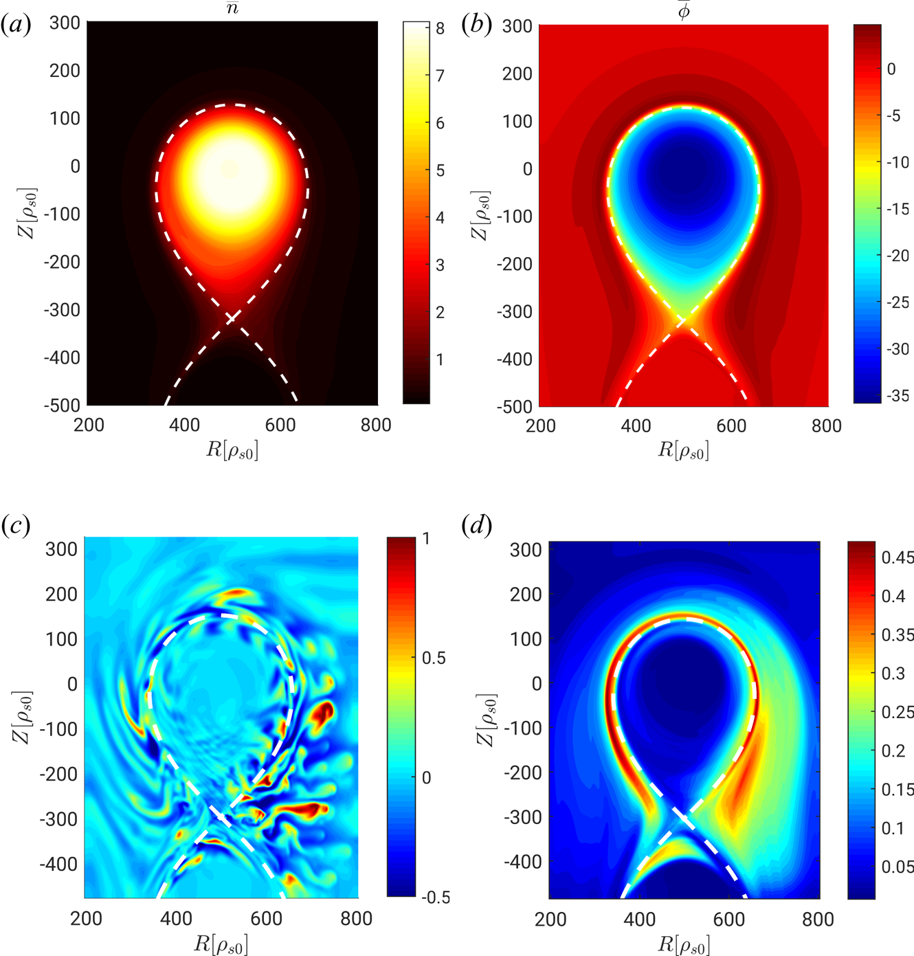
Figure 2. Equilibrium density  $(a)$, equilibrium electrostatic potential $(b)$, a snapshot of the relative density fluctuations $(c)$ and the normalized standard deviation of the density fluctuations $(d)$ for the simulation with $s_{T0} = 0.15$ and $\nu _0 = 0.2$. The dashed white line represents the separatrix.
By varying the heat source and the collisionality through the parameters  $s_{T0}$ and $\nu _0$, respectively, three different turbulent regimes are identified in our simulations: (i) a regime of developed turbulent transport, which we link to the low-confinement mode (L-mode) of tokamak operation, discussed in § 4.1; (ii) a regime of suppressed turbulent transport, with similarities to the high-confinement mode (H-mode), discussed in § 4.2; and (iii) a regime of degraded confinement with catastrophically high turbulent transport, which we associate with the crossing of the density limit and discuss in § 4.3. While the transition from the developed to the suppressed transport regime is rather sharp, the transition to the degraded confinement regime is gradual.
Typical radial profiles at the LFS midplane of the equilibrium pressure, electrostatic potential and  $\boldsymbol {E}\times \boldsymbol {B}$ shear are shown in figure 3 for the three regimes. We consider the simulations with $s_{T0}=0.9$ and $\nu _0=0.2$ (suppressed transport regime), $\nu _0=0.6$ (developed transport regime), and $\nu _0=2.0$ (degraded confinement regime). In the suppressed transport regime, the electrostatic potential drops significantly inside the separatrix, generating a strong $\boldsymbol {E}\times \boldsymbol {B}$ shear across it. This is associated with a steep gradient in the density, electron and ion temperatures. With respect to the suppressed transport regime, in the developed transport regime the electrostatic potential across the separatrix is flatter, the equilibrium $\boldsymbol {E}\times \boldsymbol {B}$ shear is reduced, transport due to turbulence is larger and, consequently, the density and temperature gradient at the tokamak edge is significantly lower. In the degraded confinement regime, turbulent transport is extremely large, leading to a flat profile of density, temperature and electrostatic potential. We note that analogous transitions can be observed by varying the heat source while keeping $\nu _0$ constant.
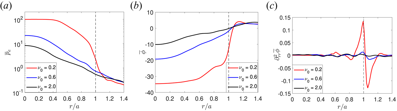
Figure 3. Radial profiles at the LFS midplane of the equilibrium pressure  $(a)$, equilibrium electrostatic potential $(b)$, and equilibrium $\boldsymbol {E}\times \boldsymbol {B}$ shear $(c)$ for the simulation with $s_{T0}=0.15$ and $\nu _0=0.2$ (suppressed transport regime), $\nu _0=0.6$ (developed transport regime), and $\nu _0=2.0$ (degraded confinement regime). The radial coordinate is normalized to the radial position $a$ of the separatrix at the midplane.
Typical snapshots of plasma turbulence in the three transport regimes can be seen in figure 4, where the relative density fluctuations and the corresponding normalized standard deviation are shown for the three simulations we are considering. In the case of  $\nu _0=0.2$, turbulence is localized near the separatrix and, as a consequence of being sheared apart by the strongly varying $\boldsymbol {E}\times \boldsymbol {B}$ radial profile, turbulent structures are elongated along the $\boldsymbol {\nabla }\chi$ direction, effectively reducing the cross-field transport. The radial extension of turbulent structures is larger for $\nu _0=0.6$ and $\nu _0=2.0$. In particular, at $\nu _0=2.0$, turbulent structures penetrate into the core region. This is in agreement with experimental observations of density fluctuations when the density limit is approached (LaBombard et al. Reference LaBombard, Boivin, Greenwald, Hughes, Lipschultz, Mossessian, Pitcher, Terry and Zweben2001). In addition, in the case of $\nu _0=0.2$, density fluctuations are generated at both the LFS and high-field side, while, in the other two cases, turbulence mainly develops at the LFS.
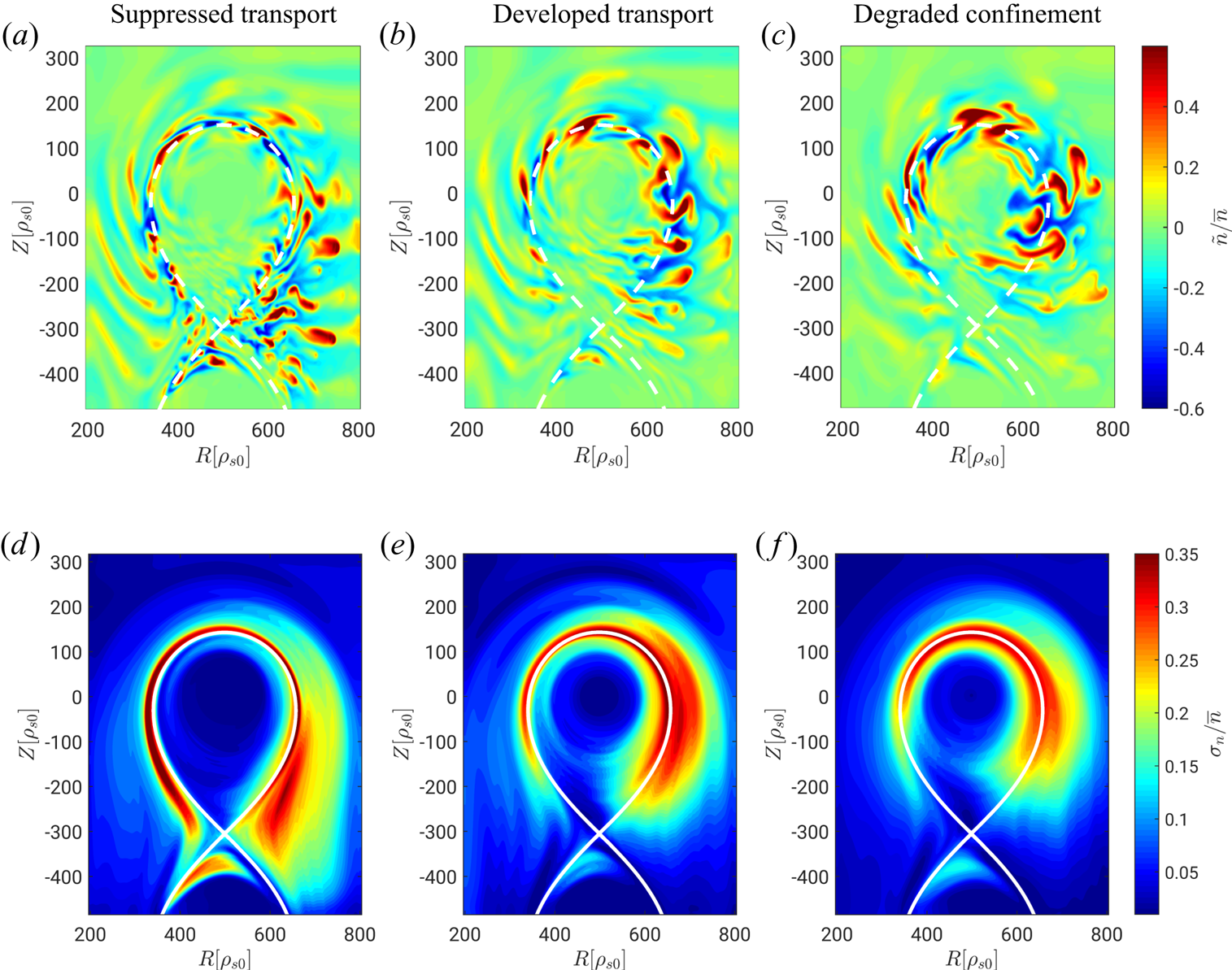
Figure 4. Typical snapshots of the relative density fluctuations (a–c) and normalized standard deviation of the density fluctuations (d–f) for three simulations with  $s_{T0}=0.15$ in the suppressed transport regime, $\nu _0=0.2$ (a,d), developed transport regime, $\nu _0=0.6$ (b,e), and degraded confinement regime, $\nu _0=2.0$ (c,f).
In order to highlight the difference in the confinement properties between the different regimes, we compute the electron energy confinement time,  $\tau _E=(3(\int _{A_{\text {LCFS}}} \bar {p}_e\,\mathrm {d}R\,\mathrm {d}Z)/2)/\!\int _{A_{\text {LCFS}}} s_p\,\mathrm {d}R\,\mathrm {d}Z$, for the set of simulations considered in the present study, at different values of $S_{T}$ and $\nu _0$ (see figure 5). At a given $\nu _0$ or $S_T$, we note that the simulations in the suppressed transport regime have a higher energy confinement time than the simulations in the developed transport regime. For this reason, we also refer to the developed transport regime as the L-mode and to the suppressed transport regime as the H-mode. The energy confinement time increases by a factor of two from the L-mode to the H-mode, as observed in experiments. In addition, as a consequence of the larger fluctuations, the energy confinement time is lower in the degraded confinement regime than in the developed transport regime.
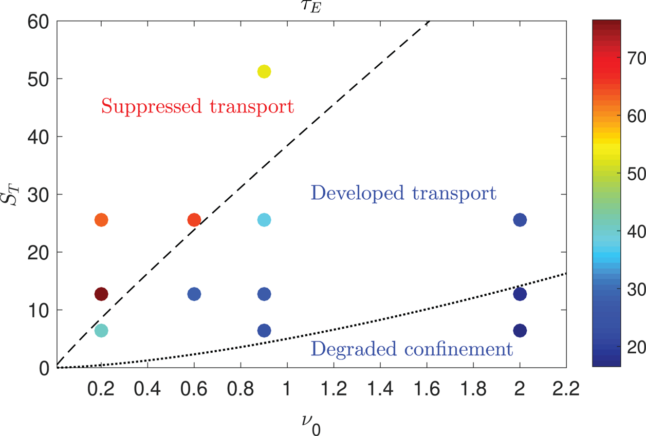
Figure 5. Electron energy confinement time for the set of simulations performed for the present study. The dashed black line represents the heat source threshold to access the suppressed transport regime (derived in § 5.1, see (5.7)), while the dotted black line represents the heat source threshold to access the degraded confinement regime (derived in § 5.2, see (5.11)).
A detailed analysis of the three regimes is reported in § 4. The power thresholds to access the suppressed transport regime and the degraded confinement regime, both displayed in figure 5 as a function of  $\nu _0$, are discussed in § 5.
4 Turbulent transport regimes at the tokamak edge
In this section, we analyse separately the three transport regimes revealed by our simulations. The mechanisms driving turbulence are studied and an analytical expression of the edge equilibrium pressure gradient length is derived for the different transport regimes.
4.1 Developed transport regime (L-mode)
We start by considering the regime of developed transport, which we associate with the L-mode. In this regime, shown by our simulations at intermediate heat source values and intermediate values of collisionality (see figure 5), the shear flow is negligible and turbulent transport results from the nonlinear development of interchange-driven electrostatic ballooning modes (Mosetto et al. Reference Mosetto, Halpern, Jolliet, Loizu and Ricci2013). This can be verified by removing the interchange drive from the simulations, i.e. by toroidally averaging the term proportional to  $C(p_e+\tau p_i)$ in (2.2). The result of this test is displayed in figure 6, where a snapshot of the electron temperature, with and without the interchange drive, is shown for a simulation in the L-mode regime ( $s_{T0} = 0.075$ and $\nu _0 = 0.9$). Plasma turbulence is strongly suppressed when the term $C(p_e+\tau p_i)$ is toroidally averaged and, as a consequence, an increase of the equilibrium temperature and pressure gradients is observed. On the other hand, turbulent structures and plasma profiles do not change significantly when the Reynolds stress, i.e. the term $\rho _*^{-1}[\phi ,\omega ]/B$ appearing in (2.2), is toroidally averaged (see figure 6). This shows that the $\boldsymbol {E}\times \boldsymbol {B}$ shear and the KH instability do not play a major role in the developed transport regime.
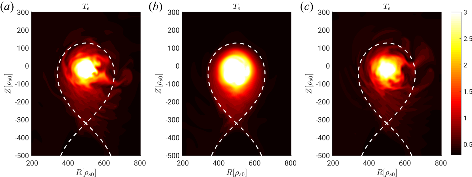
Figure 6. A typical snapshot of the electron temperature for the simulation with  $s_{T0}=0.075$ and $\nu _0=0.9$ $(a)$. Snapshots of simulations with the same parameters but the interchange drive $C(p_e+\tau p_i)$ term in (2.2) toroidally averaged $(b)$ and with the KH drive term $\rho _*^{-1} [\phi ,\omega ]/B$ in (2.2) toroidally averaged $(c)$.
In order to provide an analytical estimate of the pressure gradient length in the edge, we follow a procedure similar to the one described by Ricci, Rogers & Brunner (Reference Ricci, Rogers and Brunner2008), and we balance the perpendicular heat flux crossing the separatrix with the heat source integrated over the volume inside the LCFS. The simulations show that the equilibrium cross-field heat flux near the separatrix is negligible with respect to the turbulent one,  $\bar {p}_e\partial _{\chi }\bar {\phi } \ll \overline{\tilde {p}_e\partial _{\chi }\tilde {\phi}}$ ( $\partial _{\chi }$ denotes the derivative along $\boldsymbol {\nabla }\chi$). Therefore, we focus on the perpendicular turbulent transport, ${q_{\psi } \simeq \overline{\tilde {p}_e\partial _{\chi }\tilde {\phi }}}$, at the LCFS. The quantity $\partial _{\chi }\tilde {\phi }$ is estimated from the leading terms of the linearized electron pressure equation, which is obtained by linearizing and summing (2.1) and (2.5):
 \begin{equation} \partial_t \tilde{p}_e \sim \rho_*^{-1} \partial_{\psi} \bar{p}_e \partial_{\chi}\tilde{\phi} \end{equation}
(the curvature and parallel gradient terms appearing in (2.1) and (2.5) are significantly smaller than the terms we retain). In (4.1), we estimate the time derivative as the growth rate of the ballooning instability driving the transport,  $\gamma _i=\sqrt {2 \bar {T}_e/(\rho _*L_p)}$. We also approximate $\partial _{\psi } \bar {p}_e \simeq \bar {p}_e/L_p$, $L_p$ being the equilibrium pressure gradient length. The resulting expression of $\partial _{\chi }\tilde {\phi }$ can then be used to evaluate the cross-field interchange-induced heat flux as
 \begin{equation} q_{\psi,i}\sim \rho_*\gamma_i\frac{\tilde{p}_e^2}{\bar{p}_e}L_p. \end{equation}
The amplitude of the pressure fluctuations appearing in (4.2) can be estimated by observing that the growth of the linearly unstable modes saturates when the instability drive is removed from the system, i.e.  $k_{\psi } \tilde {p}_e \sim \bar {p}_e/L_p$ (Ricci et al. Reference Ricci, Rogers and Brunner2008; Ricci & Rogers Reference Ricci and Rogers2013). The perpendicular heat flux is then written as
 \begin{equation} q_{\psi,i}\sim\rho_*\frac{\gamma_i}{k_{\psi,i}^2}\frac{\bar{p}_e}{L_p}. \end{equation}
Non-local linear calculations show that  $k_{\psi ,i}\simeq \sqrt {k_{\chi ,i}/L_p}$ (Ricci et al. Reference Ricci, Rogers and Brunner2008). The poloidal wavenumber of the ballooning instability $k_{\chi ,i}$ can then be obtained by balancing the interchange driving and the parallel current terms in (2.2). In the parameter regime of our simulations, turbulence is driven by resistive ballooning mode (Mosetto et al. Reference Mosetto, Halpern, Jolliet, Loizu and Ricci2013). In this case, the resistivity limits the parallel current (Halpern et al. Reference Halpern, Ricci, Labit, Furno, Jolliet, Loizu, Mosetto, Arnoux, Gunn and Horacek2013a, Reference Halpern, Ricci, Jolliet, Loizu and Mosetto2014). This leads to $k_{\chi ,i} = (\bar {n}\nu q_{95}^2\sqrt {\gamma _i})^{-1/2}$. As a consequence, (4.3) becomes
 \begin{equation} q_{\psi,i}\sim \rho_*^{1/4}\sqrt{\bar{n}\nu q_{95}^2}\left(\frac{2\bar{T}_e}{L_p}\right)^{3/4}\bar{p}_e. \end{equation}
In order to derive the pressure scale length, we note that the heat source integrated over the poloidal plane inside the LCFS corresponds, approximately, to the perpendicular turbulent heat flux crossing the LCFS on a poloidal plane:
 \begin{equation} S_p(R,Z) \simeq \oint_{\text{LCFS}} q_{\psi,i}(R,Z)\,\mathrm{d}l. \end{equation}
In order to perform the integral on the right-hand side of (4.5), we note that turbulent transport is driven by ballooning modes that develop in the bad-curvature region (see figure 6). As a consequence, we assume that  $q_{\psi ,i}(R,Z)$ has a constant value at the LCFS on the LFS and vanishes at the high-field side, i.e.
 \begin{equation} S_p\sim\frac{L_{\chi}}{2}q_{\psi,i}, \end{equation}
where  $L_{\chi }= \oint _{\text {LCFS}}\,\mathrm {d}l$ is the length of the LCFS poloidal circumference. The edge equilibrium pressure gradient length is derived using (4.4) and (4.6), that is
 \begin{equation} L_{p,i} \sim \left[\frac{\rho_*}{2}(\nu q_{95}^2 \bar{n})^2\left(\frac{L_{\chi}}{S_p}\bar{p}_e\right)^4\right]^{1/3}\bar{T}_e, \end{equation}
where  $\bar {n}$, $\bar {T}_e$ and $\bar {p}_e$ are evaluated at the LCFS.
In figure 7, the ratio of  $L_p$, the equilibrium pressure gradient length directly obtained from the simulations, to $L_{p,i}$, the interchange estimate in (4.7), is displayed for the different values of $S_{T}$ and $\nu _0$ considered in the present study. At low values of $S_T$ and high values of $\nu _0$, $L_p/L_{p,i}\simeq 1$, revealing a good agreement between the analytical estimate in (4.7) and the simulation result. Hence, in the developed transport regime (as well as in the degraded confinement regime, as discussed in § 4.3), turbulence is driven by the interchange instability, the effect of the shear flow not being significant. In addition, since the formation of a pedestal is not observed in this regime, we associate this parameter region with the L-mode. On the other hand, for high values of the heat source and low values of $\nu _0$, the pressure gradient length of the simulations is larger than the value predicted by (4.7), $L_p/L_{p,i} > 1$, meaning that a mechanism different from the interchange instability is responsible for driving turbulent transport and setting the equilibrium pressure gradient length.

Figure 7. Ratio of  $L_p$, the equilibrium pressure gradient length directly obtained from the simulations, to $L_{p,i}$, the estimate in (4.7) based on the assumption that transport is driven by the interchange instability, for all the simulations considered in the present study. The dashed black line represents the heat source threshold to access the suppressed transport regime (see (5.7)), while the dotted black line represents the threshold to access the degraded confinement regime (see (5.11)).
It should be noted that, despite being still described as the result of the development of the interchange instability, transport might become catastrophically large at high values of  $\nu _0$ and low heat source values, with turbulent eddies that extend from the edge towards the tokamak core, a behaviour that we associate with the crossing of the density limit and we identify as the degraded confinement regime.
4.2 Suppressed transport regime (H-mode)
As shown in figure 3, the equilibrium edge electrostatic potential profile in the suppressed transport regime is significantly different from the one in the developed transport regime. This has strong consequences on the nature of turbulent transport. Hence, we focus on the mechanisms that set the  $\bar {\phi }$ profile.
Inside the LCFS, the radial electric field is proportional to the ion pressure gradient,  $\partial _r \bar \phi \sim -\partial _r \bar {p}_i/\bar {n}$, as experimentally observed (e.g. Schirmer et al. Reference Schirmer, Conway, Zohm and Suttrop2006; McDermott et al. Reference McDermott, Lipschultz, Hughes, Catto, Hubbard, Hutchinson, Granetz, Greenwald, LaBombard and Marr2009) and theoretically explained (e.g. Zhu, Francisquez & Rogers Reference Zhu, Francisquez and Rogers2017). On the other hand, ambipolarity of the plasma flow at the sheath imposes that the electrostatic potential is proportional to the electron temperature, $\bar {\phi } \sim \varLambda \bar {T}_e$, in the SOL, as discussed by Stangeby (Reference Stangeby2000) and Loizu et al. (Reference Loizu, Ricci, Halpern, Jolliet and Mosetto2013). Therefore, $\bar {\phi }$ radially increases as one moves from the magnetic axis towards the LCFS ( $-\partial _r \bar {p}_i/\bar {n} > 0$) and then decreases from the LCFS towards the far SOL ( $\partial _r\bar {T}_e<0$). It follows that $\bar {\phi }$ peaks near the separatrix (see figure 3b). As $s_{T0}$ increases or $\nu _0$ decreases, both $T_e$ and $T_i$ increase and, as a consequence, also the $\boldsymbol {E}\times \boldsymbol {B}$ shear flow across the LCFS increases (see figure 3c). Because of the $\boldsymbol {E}\times \boldsymbol {B}$ shear, the turbulent eddies in the edge resulting from the interchange instability are sheared along the $\boldsymbol {\nabla } \chi$ direction. Furthermore, when the shearing rate, $\rho _*^{-1}\partial _{rr}^2\bar {\phi }$, is comparable to $\gamma _i$, ballooning turbulence is nonlinearly suppressed (Burrell Reference Burrell1997; Terry Reference Terry2000). At the same time, the $\boldsymbol {E}\times \boldsymbol {B}$ shear provides the drive of the KH instability through the Reynolds stress (Myra et al. Reference Myra, D'Ippolito, Russell, Umansky and Baver2016). Indeed, our simulations show that, for values of the heat source sufficiently high, when $\rho _*^{-1}\partial _{rr}^2\bar {\phi } > \gamma _i$, the interchange instability is suppressed in the edge and the KH instability becomes the primary instability driving the turbulent transport (Rogers & Dorland Reference Rogers and Dorland2005; Myra et al. Reference Myra, D'Ippolito, Russell, Umansky and Baver2016).
Figure 8 displays a typical snapshot of the electron temperature for a simulation in the suppressed transport regime ( $s_{T0}=0.6$ and $\nu _0=0.9$) and compares it to two simulations having the same parameters, but with the KH and ballooning drives removed. Turbulence is strongly suppressed when the Reynolds stress is toroidally averaged. On the other hand, no significant effect on turbulence is noticed when the interchange drive is removed. This shows that the KH instability is the main drive of turbulent transport and, consequently, regulates the equilibrium pressure gradient in the suppressed transport regime.
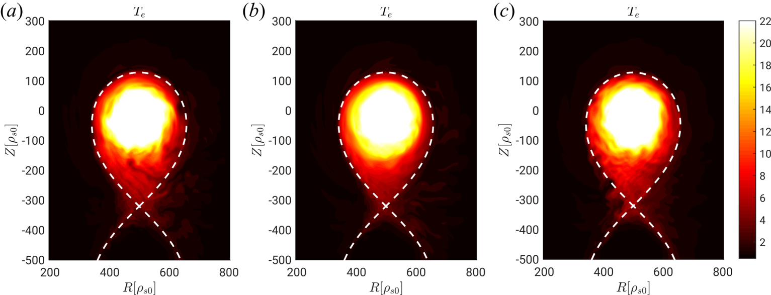
Figure 8. A typical snapshot of the electron temperature for the simulation with  $s_{T0}=0.6$ and $\nu _0=0.9$ $(a)$. Snapshots of simulations with the same parameters but the KH drive term $\rho _*^{-1} [\phi ,\omega ]/B$ in (2.2) toroidally averaged $(b)$ and with the interchange drive term $C(p_e+\tau p_i)$ in (2.2) toroidally averaged $(c)$.
An analytical estimate of the equilibrium pressure gradient length in the edge when turbulence is driven by the KH instability can be derived by following a procedure similar to the one detailed in § 4.1 and discussed for a linear device by Rogers & Ricci (Reference Rogers and Ricci2010). The growth rate of the KH instability is proportional to the  $\boldsymbol {E}\times \boldsymbol {B}$ shear (Myra et al. Reference Myra, D'Ippolito, Russell, Umansky and Baver2016), $\gamma _{\text {KH}} \sim \rho _*^{-1}\partial _{rr}^2 \bar {\phi } \sim \rho _*^{-1}\bar {T}_e/L_p^2$, having assumed $L_{\phi } \sim L_p$. The KH mode being a global one, the size of the turbulent eddies it generates is comparable to the pressure gradient length, $k_{\psi ,\text {{KH}}} \sim 1/L_p$. Therefore, similarly to (4.3), the KH-driven heat flux can be expressed as
 \begin{equation} q_{\psi,\text{{KH}}} \sim \frac{\bar{T}_e \bar{p}_e}{L_p}. \end{equation}
By balancing the heat source integrated over the region inside the LCFS and the perpendicular turbulent heat flux crossing the LCFS, similarly to (4.5), but assuming that  $q_{\psi ,\text {{KH}}}$ is approximately uniform along the LCFS, we obtain
 \begin{equation} L_{p,\text{{KH}}} \sim \frac{\bar{p}_e \bar{T}_e}{4S_p}L_{\chi}, \end{equation}
where  $\bar {T}_e$ and $\bar {p}_e$ are evaluated at the LCFS.
The ratio of  $L_p$, the equilibrium pressure gradient length directly obtained from the simulations, to $L_{p,\text {{KH}}}$, the estimate in (4.9), is displayed in figure 9 for the different simulations considered in the present study. At large values of $S_T$ and small values of $\nu _0$, a region can be identified where $L_{p,\text {{KH}}}$ well reproduces the simulation results. In fact, the results of figures 7 and 9 show that turbulent transport is driven by the KH instability in the suppressed transport regime, otherwise the interchange instability regulates the equilibrium pressure gradient length. Furthermore, we note that $L_p>L_{p,\text {{KH}}}$ in the ballooning-driven parameter region, while $L_p>L_{p,i}$ in the suppressed transport regime, as expected from the fact that the mode driving turbulence minimizes the pressure gradient.

Figure 9. Ratio of  $L_p$, the equilibrium pressure gradient length directly obtained from the simulations, to $L_{p,\text {{KH}}}$, the estimate in (4.9) based on the assumption that the transport is driven by the KH instability, for all the simulations considered in the present study. The dashed black line represents the heat source threshold to access the suppressed transport regime (see (5.7)), while the dotted black line represents the threshold to access the degraded confinement regime (see (5.11)).
The suppressed transport regime shows some of the main key aspects observed experimentally in H-mode discharges, such as the presence of a strong sheared flow (see figure 3c), the reduction of the turbulence level with respect to the L-mode that leads to the formation of a transport barrier near the separatrix (see figure 3a), and the increase of the energy confinement time (see figure 5). All this occurs when a power threshold is exceeded, as detailed in § 5.1. We therefore associate the suppressed transport regime with the H-mode of tokamak operation.
4.3 Degraded confinement regime
Figures 4 and 5 show that plasma turbulence and confinement properties strongly vary also within the interchange-driven turbulent regime. In general, for high values of  $\nu _0$ and low values of $s_{T0}$, poor confinement properties and a catastrophically large turbulent transport are observed. Indeed, in this parameter regime, despite being described as the nonlinear development of a ballooning mode, turbulence results in high-level fluctuations, with amplitude comparable to the equilibrium quantity, that propagate from the edge to the core region, as shown in figure 4. This is due to the fact that the radial size of the turbulent structures increases with $\nu _0$, since $k_{\chi ,i} \propto \nu _0^{-1/2}$ and $k_{\psi ,i} \simeq \sqrt {k_{\chi ,i}/L_{p,i}} \propto \nu _0^{-7/12}$. Figure 10 shows the radial extension of turbulent eddies normalized to the tokamak minor radius for the different simulations considered in the present study. In particular, if the value of $\nu _0$ is sufficiently large and $s_{T0}$ sufficiently small, turbulent eddies appear to have a size comparable to the tokamak minor radius, i.e. $k_{\psi } a\sim 1$. As a consequence, they extend towards the core region and lead to a very large cross-field turbulent transport throughout the closed field line region. In these conditions, the core temperature can significantly drop and magnetohydrodynamic modes, which are beyond the description provided by our model, can play an important role (Greenwald et al. Reference Greenwald, Terry, Wolfe, Ejima, Bell, Kaye and Neilson1988; Greenwald Reference Greenwald2002). As already mentioned in § 3, the degraded confinement regime is linked to high values of the density and we associate it with the crossing of the density limit, in agreement with the result of Hajjar et al. (Reference Hajjar, Diamond and Malkov2018). Experimental evidences that the density limit is due to an increase of edge collisionality, proportional to $\nu _0$ in the model considered, are reported from the TJ-K stellarator (Schmid et al. Reference Schmid, Manz, Ramisch and Stroth2017).
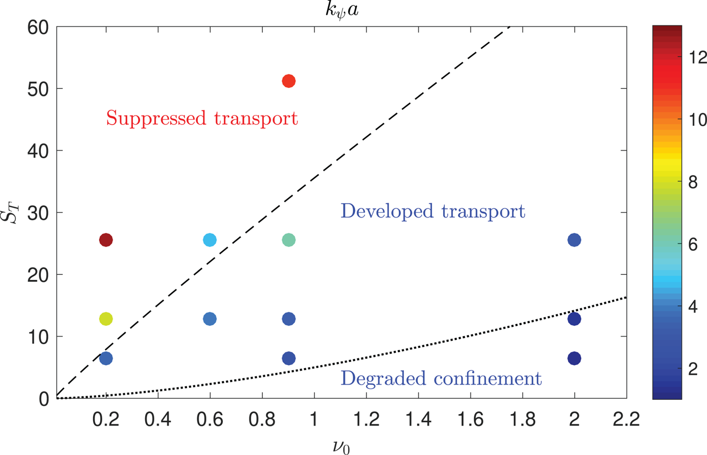
Figure 10. Radial wavenumber computed from the correlation length of turbulent eddies, normalized to the tokamak minor radius, for all the simulations considered in the present study. The dashed black line represents the heat source threshold to access the suppressed transport regime (see (5.7)), while the dotted black line represents the threshold to access the degraded confinement regime (see (5.11)).
Three main effects are observed when crossing the density limit. First, the  $\boldsymbol {E}\times \boldsymbol {B}$ shear near the separatrix in the degraded confinement regime is even weaker than in the developed transport regime, as shown in figure 3(c). This is in agreement with recent experiments that show how the edge shear flow collapses when the density limit is approached (Hong et al. Reference Hong, Tynan, Diamond, Nie, Guo, Long, Ke, Wu, Yuan and Xu2017). Therefore, the $\boldsymbol {E}\times \boldsymbol {B}$ shear is an important quantity not only to explain the transition from the developed transport regime to the suppressed transport regime, but also to recognize the crossing of the density limit. Second, the degraded confinement regime is characterized by a flatter equilibrium density profile in the SOL with respect to the developed and suppressed transport regimes (see figure 11). In fact, the blob size increases with the collisionality (D'Ippolito et al. Reference D'Ippolito, Myra and Zweben2011; Nespoli et al. Reference Nespoli, Furno, Labit, Ricci, Avino, Halpern, Musil and Riva2017; Beadle & Ricci Reference Beadle and Ricci2020), leading to an enhancement of the cross-field turbulent transport in the far SOL. The density profile becomes flatter with no clear distinction between the edge, near SOL and far SOL. Experimental observations of the flattening of the density profiles as the density increases towards the density limit are reported by LaBombard et al. (Reference LaBombard, Boivin, Greenwald, Hughes, Lipschultz, Mossessian, Pitcher, Terry and Zweben2001). Third, the large-amplitude fluctuations that extend towards the core region lead to a strong enhancement of cross-field turbulent transport and the loss of confinement.
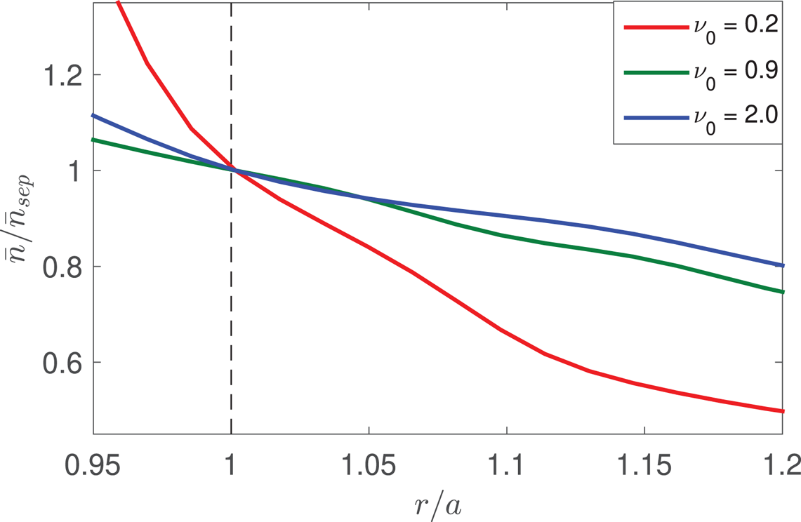
Figure 11. Equilibrium density radial profile at the outboard midplane for simulations at  $s_{T0}=0.075$ and various values of $\nu _0$.
5 Transition threshold between transport regimes
In this section, we focus on the transition from the developed transport regime to the suppressed transport regime, which we associate with the L–H transition, and from the developed transport regime to the degraded confinement regime, which we associate with the crossing of the density limit. Analytical estimates of the heat source threshold to access the suppressed transport regime and of the density threshold to access the degraded confinement regime are derived.
5.1 Heat source threshold to access the suppressed transport regime
The transition from the L-mode to the H-mode occurs when  $L_{p,i}\simeq L_{p,{\text {{KH}}}}$, namely when the turbulent transport due to the interchange instability equals the one due to the KH instability. An estimate of $S_p$ at the transition can be derived by equating (4.7) and (4.9):
 \begin{equation} S_p^{\text{LH}}\sim \rho_* L_{\chi} \nu_0^2 q_{95}^4 \bar{n}^3/(2 \bar{T}_e), \end{equation}
where  $\bar {n}$ and $\bar {T}_e$ are evaluated at the LCFS. The relation between $\bar {T}_e$ at the LCFS and $S_p$ can be obtained by balancing $S_p$ with the parallel losses to the vessel walls. As an order of magnitude estimate, this balance can be expressed by using the integral of the heat flux over the SOL width, $\varDelta _{\text {SOL}}$, as
 \begin{equation} \int_{\varDelta_{\text{SOL}}} \bar{p}_e \bar{c}_s\, \mathrm{d}l \sim S_p, \end{equation}
having assumed to be in the sheath connected regime (i.e. no temperature drop in the divertor region) and assuming that the plasma outflows at the divertor plate with the sound speed. Furthermore, by assuming that the pressure and temperature decay exponentially in the SOL on  $L_p$ scale, (5.2) becomes
 \begin{equation} \bar{T}_e \sim \left(\frac{2 S_p}{\bar{n} L_p}\right)^{2/3}, \end{equation}
with  $\bar {T}_e$ and $\bar {n}$ evaluated at the LCFS. Equations (5.1) and (5.3) allow us to derive an analytical estimate of the heat source threshold for H-mode access,
 \begin{equation} S_p^{\text{LH}} \sim \rho_*^{7/15}(\nu_0 q_{95}^2)^{14/15} L_{\chi}^{11/15}\bar{n}^{29/15}, \end{equation}
the corresponding electron temperature at the LCFS,
 \begin{equation} T_e^{\text{LH}}\sim \rho_*^{4/15} (\nu_0 q_{95}^2)^{8/15} L_{\chi}^{2/15} \bar{n}^{8/15} , \end{equation}
and the equilibrium pressure gradient length at the transition,
 \begin{equation} L_p^{\text{LH}}\sim \rho_*^{1/15} (\nu_0 q_{95}^2)^{2/15} L_{\chi}^{8/15} \bar{n}^{2/15}. \end{equation}
In (5.4), the increase of the heat source required to access the H-mode with  $\nu _0$ is due to the increase of cross-field turbulent transport in the developed transport regime. Indeed, $q_{\psi ,i}$ is proportional to $\nu _0^{1/2}$ (see (4.4)) and $L_{p,i}$ is proportional to $\nu _0^{2/3}$ (see (4.7)).
We now compare our analytical estimate with the simulation results. For this purpose, we express (5.4) in terms of  $S_T$, by using $S_T^{\text {LH}}\simeq S_p^{\text {LH}}/\bar {n}$, and we obtain
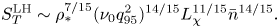 \begin{equation} S_T^{\text{LH}} \sim \rho_*^{7/15}(\nu_0 q_{95}^2)^{14/15} L_{\chi}^{11/15}\bar{n}^{14/15}. \end{equation}
The analytical estimate of the threshold  $S_T^{\text {LH}}$ as a function of $\nu _0$ (assuming a constant value for the normalized density $\bar {n}$ at the LCFS) is displayed in figure 9, showing a very good agreement between the analytical prediction of (5.7) and the simulation results.
We also link our L–H transition with experimental observations. In order to identify the scaling of  $S_p^{\text {LH}}$ with the main experimental parameters, we write the power threshold in (5.4) in physical units as
 \begin{align} P_{\text{{LH}}} = 2{\rm \pi} R_0 S_p^{\text{LH}} &\simeq 9\times 10^7\left(\frac{m_e}{m_i}\right)^{9/15} n^{29/15} R_0^{22/15} q_{95}^{28/15} a^{11/15} B_T^{-11/15}\nonumber\\ &\simeq 9\times 10^7\left(\frac{m_e}{m_i}\right)^{0.6}n^{1.9} R_0^{1.5} q_{95}^{1.9}a^{0.7}B_T^{-0.7}, \end{align}
with the  $2{\rm \pi} R_0$ factor taking into account the integration of the heat source along the toroidal direction, having imposed $L_{\chi }\sim 2{\rm \pi} a$, and the density at the LCFS being expressed in units of $10^{20}\ \textrm {m}^{-3}$. The scaling law in (5.8) correctly reproduces the isotope effect observed in experiments (Righi et al. Reference Righi, Bartlett, Christiansen, Conway, Cordey, Eriksson, De Esch, Fishpool, Gowers and De Haas1999; Maggi et al. Reference Maggi, Weisen, Hillesheim, Chankin, Delabie, Horvath, Auriemma, Carvalho, Corrigan and Flanagan2017) and also found in previous theoretical investigations (De Dominici et al. Reference De Dominici, Fuhr, Beyer, Bourdelle, Chôné, Cianfrani, Falchetto, Garbet and Sarazin2019). The dependence on $a$ and $R_0$ shows a good agreement with the experimental scaling law in (1.1). The exponent of the density in (5.8) is a factor of approximately 2.7 larger than the one predicted by the experimental scaling law in (1.1), although we remark that the density in (5.8) is evaluated at the LCFS, while the density in (1.1) denotes the line-averaged density. The power threshold in (5.8) depends inversely on the toroidal magnetic field, while the experimental scaling law in (1.1) shows a direct dependence on $B_T$. Moreover, in contrast to the experimental scaling law in (1.1), the power threshold in (5.8) depends on $q_{95}$.
As an example of the evaluation of (5.8) in experimental conditions, we consider the value of the power threshold predicted for typical parameters of the TCV tokamak ( $a=0.25\ \textrm {m}$, $R_0=0.88\ \textrm {m}$, line-averaged density $n_e\simeq 4\times 10^{19}\ \textrm {m}^{-3}$, density at the LCFS $n\simeq 2\times 10^{19}\ \textrm {m}^{-3}$, $B_T\simeq 1.4\ \textrm {T}$, and $q_{95} \simeq 4$). The estimate in (5.8) gives $P_{\text {{LH}}}\simeq 142\ \textrm {kW}$, a power threshold that has the same order of magnitude as the experimental TCV power threshold, $P_{\text {{LH}}}\simeq 260\ \textrm {kW}$ (e.g. Scaggion et al. Reference Scaggion, Martin and Reimerdes2012; Martin et al. Reference Martin, Behn, Furno, Labit and Reimerdes2014).
Experimental measurements show that the power to access the H-mode is lower when the ion- $\boldsymbol {\nabla } B$ drift direction is towards the X-point, rather than away from it (ASDEX Team 1989). In order to study the dependence of the heat source threshold on the ion- $\boldsymbol {\nabla } B$ drift direction, we consider two simulations where we vary the direction of the toroidal magnetic field while keeping the same direction of the plasma current and other parameters the same. In particular, we consider $s_{T0}=0.3$ and $\nu _0=0.9$, parameters close to the L–H transition when the ion- $\boldsymbol {\nabla } B$ drift direction points upwards (unfavourable for H-mode access). The equilibrium density, temperature and $\boldsymbol {E}\times \boldsymbol {B}$ shear profiles at the LFS midplane do not show significant differences between the simulations with favourable and unfavourable ion- $\boldsymbol {\nabla } B$ drift direction, both simulations belonging to the developed transport regime. Therefore, at least in the case analysed, the power threshold to access the H-mode is independent of the toroidal magnetic field direction in our model. The discrepancy between experimental and simulation observations may be due to the absence of kinetic effects involving passing and trapped particles; among these we mention the effects of ion orbit loss, which can be important in establishing the dependence of the L–H transition on the ion- $\boldsymbol {\nabla } B$ drift direction (Stoltzfus-Dueck Reference Stoltzfus-Dueck2012; Boedo et al. Reference Boedo, DeGrassie, Grierson, Stoltzfus-Dueck, Battaglia, Rudakov, Belli, Groebner, Hollmann and Lasnier2016), as also pointed out by XGC1 simulations (Ku et al. Reference Ku, Chang, Hager, Churchill, Tynan, Cziegler, Greenwald, Hughes, Parker and Adams2018).
Experimental observations (Snipes et al. Reference Snipes, Boivin, Christensen, Fiore, Garnier, Goetz, Golovato, Graf, Granetz and Greenwald1996; Thomas et al. Reference Thomas, Groebner, Burrell, Osborne and Carlstrom1998) and theoretical models (Hinton Reference Hinton1991; Drake et al. Reference Drake, Lau, Guzdar, Hassam, Novakovski, Rogers and Zeiler1996) point out the presence of hysteresis on the power threshold for the L–H transition, i.e. having entered the H-mode conditions, the hysteresis allows for a decrease of the power below the threshold for H-mode access without inducing the H–L transition. The presence of hysteresis in our simulations is investigated by performing a set of simulations at  $\nu _0=0.2$ and various values of $s_{T0}$ in the proximity of the threshold to access the suppressed transport regime (more precisely we consider $s_{T0}= 0.045, 0.055, 0.065, 0.075, 0.085, 0.095, 0.105$). Starting from a simulation in the developed transport regime, $s_{T0}$ is progressively increased from 0.045 to 0.105 where the transition to the suppressed transport regime occurs. Then, using the simulation at $s_{T0}=0.105$ in the suppressed transport regime as initial condition, we perform a second set of simulations where $s_{T0}$ is progressively reduced, observing the H–L transition at $s_{T0} \simeq 0.065$ (see figure 12). Therefore, the transition from the developed transport regime to the suppressed transport regime occurs at a higher value of the heat source than the reverse transition, thus pointing out the presence of hysteresis in the considered model.
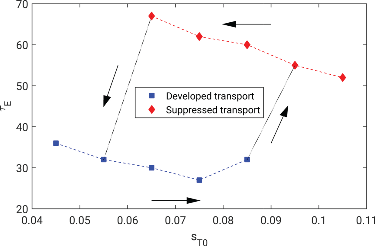
Figure 12. Energy confinement time for simulations with  $\nu _0=0.2$ and various values of $s_{T0}$. Simulations in the developed transport regime are denoted by blue squares and in the suppressed transport regime by red diamonds. Starting from a simulation in the developed transport regime, $s_{T0}$ is progressively increased from 0.045 to 0.105. The transition to the suppressed transport regime occurs approximately at $s_{T0}\simeq 0.085$. The heat source is then progressively reduced until the reverse transition occurs, approximately at $s_{T0}\simeq 0.065$. The transitions are represented as dotted black lines.
The presence of hysteresis can be explained as follows. In the suppressed transport regime, the  $\boldsymbol {E}\times \boldsymbol {B}$ shear is strong near the separatrix and the turbulent transport is mainly driven by the KH instability. As the heat source decreases, the equilibrium pressure gradient decreases (see (4.9)) as well as the $\boldsymbol {E}\times \boldsymbol {B}$ shear near the separatrix. However, the $\boldsymbol {E}\times \boldsymbol {B}$ shear remains sufficiently strong to stabilize ballooning modes, thus allowing for a decrease of the heat source below the L–H transition threshold with no collapse of the $\boldsymbol {E}\times \boldsymbol {B}$ shear. This collapse is suddenly followed by the onset of the interchange instability, with the developed transport regime eventually reached.
As an aside observation of figure 12, we note that, within the same transport regime, the energy confinement time decreases as the heat source increases, the only exception being the simulation at  $s_{T0}=0.085$ in the developed transport regime, which is in the proximity of the transition. The decrease of the energy confinement time following the increase of the heat source is also observed in many experiments (Yushmanov et al. Reference Yushmanov, Takizuka, Riedel, Kardaun, Cordey, Kaye and Post1990; Cordey et al. Reference Cordey, Thomsen, Chudnovskiy, Kardaun, Takizuka, Snipes, Greenwald, Sugiyama, Ryter and Kus2005).
5.2 Density threshold to access the degraded confinement regime
In our simulations, the transition to the degraded confinement regime occurs gradually as the edge fluctuations present in the developed transport regime reach a size comparable to the system size,  $1/k_{\psi }\sim a$, and the equilibrium pressure gradient length becomes comparable to the tokamak minor radius, $L_p\sim a$. This last observation can be considered as a condition to access the regime of degraded confinement. By assuming interchange-driven turbulent transport, this condition can be expressed as
 \begin{equation} a\sim L_{p,i}\sim \left[\frac{\rho_*}{2}(\nu q_{95}^2 \bar{n})^2\left(\frac{2{\rm \pi} a}{S_p}\bar{p}_e\right)^4\right]^{1/3}\bar{T}_e, \end{equation}
having estimated the equilibrium pressure gradient length according to (4.7), and  $\bar {n}$ and $\bar {T}_e$ being evaluated at the LCFS. By using the estimate of the electron temperature in (5.3), we obtain
 \begin{equation} S_p\sim \rho_*^{3/4}\frac{8{\rm \pi}^3}{a^{5/4}}(\nu_0 q_{95}^2)^{3/2}\bar{n}^{5/2}. \end{equation}
In order to compare (5.10) with the simulation results, we express (5.10) in terms of  $S_T$, again using $S_p\simeq S_T/\bar {n}$, and we find
 \begin{equation} S_T \sim \rho_*^{3/4}\frac{8{\rm \pi}^3}{a^{5/4}}(\nu_0 q_{95}^2)^{3/2}\bar{n}^{3/2}. \end{equation}
The analytical prediction of temperature source threshold in (5.11) is plotted in the phase space of figure 10, by keeping constant the normalized density at the LCFS (this value is approximately constant in the simulations considered in the present study). A good agreement between the simulation results and the theoretical estimate is shown by the analysis of the radial extension of the turbulent eddies.
For comparison with experimental results, the heat source threshold in (5.10) can be written in physical units as
 \begin{equation} S_p\simeq 3.2 \left(\frac{m_i}{m_e}\right)^{1/4} \frac{a^{19/4} n^{5/2}}{I_p^3 R_0^{9/4}}, \end{equation}
where  $S_p$ is expressed in $\textrm {kW}\,\textrm {m}^{-1}$ and $n$ in $10^{20}\ \textrm {m}^{-3}$, $I_p$ is the plasma current (in MA) and we have used $q_{95}\sim 2{\rm \pi} a^2 B_T/(R_0 I_p)$. The density threshold to access the degraded confinement regime, corresponding to the operational density limit evaluated at the LCFS, can then be derived from (5.12) and, in physical units, takes the following form:
 \begin{equation} n \simeq 0.3 \left(\frac{m_e}{m_i}\right)^{1/10} P_{\text{sep}}^{2/5} R_0^{1/2} \frac{I_p^{6/5}}{a^{19/10}} \simeq 0.3 \left(\frac{m_e}{m_i}\right)^{0.1} P_{\text{sep}}^{0.4} R_0^{0.5} \frac{I_p^{1.2}}{a^{1.9}}, \end{equation}
where  $P_{\text {sep}}=2{\rm \pi} R_0 S_p$ is the power crossing the separatrix (in kW), with $I_p$ in MA and $n$ in $10^{20}\ \textrm {m}^{-3}$. The comparison between the analytical scaling law of (5.13) and the empirical scaling in (1.2) is not straightforward since we have expressed the density limit in terms of the density at the LCFS, while the empirical scaling refers to the line-averaged density. With this caveat in mind, we note that (5.13) reproduces the dependence on the plasma current and tokamak minor radius expected by the experimental scaling law of (1.2). The dependence on the ion mass is weak, in agreement with experimental observations that do not show evident isotope effect on the density limit (Saibene et al. Reference Saibene, Horton, Sartori, Balet, Clement, Conway, Cordey, De Esch, Ingesson and Lingertat1999). The analytical scaling law of (5.13) depends on the heat source, a feature also observed in some experiments (Stabler et al. Reference Stabler, McCormick, Mertens, Muller, Neuhauser, Niedermeyer, Steuer, Zohm, Dollinger and Eberhagen1992; Mertens et al. Reference Mertens, Kaufmann, Neuhauser, Schweinzer, Stober, Buchl, Gruber, Haas, Herrmann and Kallenbach1997). For instance, it has been experimentally found (Mertens et al. Reference Mertens, Kaufmann, Neuhauser, Schweinzer, Stober, Buchl, Gruber, Haas, Herrmann and Kallenbach1997) that, at the density limit, the density at the LCFS depends on the power crossing the separatrix as $n \propto P_{\text {sep}}^{0.6}$, in good agreement with the power dependence in (5.13). However, the analytical density threshold of (5.13) depends also on the tokamak major radius, while the empirical scaling in (1.2) is independent of it. As an example of application of (5.13), we note that the threshold density predicted for the TCV tokamak ( $a=0.25\ \textrm {m}$, $R_0=0.88\ \textrm {m}$, $I_p=1\ \textrm {MA}$ and $P_{\text {sep}}=100\ \textrm {kW}$) is $n \simeq 10^{21}\ \textrm {m}^{-3}$.
6 Conclusions
In the present paper, results of flux-driven simulations in realistic single-null geometry, carried out using the GBS code with the domain encompassing the whole tokamak to retain the core–edge–SOL interplay, are used to study the important role of sources and resistivity in driving a variety of turbulent transport regimes in the tokamak edge. Our simulations show the presence of three turbulent transport regimes: a regime of developed turbulent transport, which we link to the L-mode observed in the experiments; a regime of suppressed turbulent transport, with similarities to the H-mode; and a regime of degraded confinement, which we associate with the crossing of the density limit. The developed transport and degraded confinement regimes appear at low heat source and high resistivity, with turbulent transport driven by the interchange instability, while the suppressed transport regime appears at high heat source and low resistivity, with turbulent transport driven by the KH instability. The energy confinement time in the suppressed transport regime is a factor of approximately two higher than in the developed transport regime. An overall loss of confinement is observed in the degraded confinement regime, with strong fluctuations that reach the tokamak core. An analytical expression of the equilibrium pressure gradient length in the tokamak edge is derived for all the transport regimes.
The transition from the developed to the suppressed transport regime shows many features in common with the L–H transition observed experimentally, such as the presence of a strong sheared flow, the reduction of the turbulence level, the formation of a transport barrier near the separatrix and the presence of a power threshold. The power threshold for H-mode access derived herein is able to reproduce the isotope effect and the experimental parameter scaling of (1.1), with the exception of the toroidal magnetic field and the dependence on safety factor. In addition, no dependence of the power threshold on the ion- $\boldsymbol {\nabla } B$ direction is observed in the considered simulations. The transition from the developed to the suppressed transport regime is subject to hysteresis as it occurs at a higher value of the heat source with respect to the inverse transition. The analytical prediction of the power threshold shows a good agreement with the results of GBS simulations performed with various values of heat source and resistivity (see figure 5).
In the degraded confinement regime, found at high values of resistivity and low heat source, turbulent transport is driven by the interchange instability with turbulent eddies of size comparable to the tokamak minor radius. High-level fluctuations are generated in the core and the particle confinement time drops. We derive an analytical estimate of the density threshold to access the degraded confinement regime, which we associate with the operational Greenwald density limit. Indeed, it retrieves the main dependencies on the plasma current and tokamak minor radius observed experimentally (Greenwald Reference Greenwald2002).
Finally, we remark that the model considered in this work neglects coupling with neutrals dynamics, neoclassical and kinetic effects. Moreover, it is electrostatic and makes use of the Boussinesq approximation. These terms can definitely have an impact on the edge turbulent regimes. In fact, neutral dynamics may affect the L–H transition dynamics, as shown by Shaing & Hsu (Reference Shaing and Hsu1995), Carreras et al. (Reference Carreras, Diamond and Vetoulis1996) and Owen et al. (Reference Owen, Carreras, Maingi, Mioduszewski, Carlstrom and Groebner1998). In Chôné et al. (Reference Chôné, Beyer, Sarazin, Fuhr, Bourdelle and Benkadda2014, Reference Chôné, Beyer, Sarazin, Fuhr, Bourdelle and Benkadda2015) and Viezzer et al. (Reference Viezzer, Pütterich, Angioni, Bergmann, Dux, Fable, McDermott, Stroth and Wolfrum2013), it is shown that neoclassical terms play an important role in the radial electric field responsible for the onset of a transport barrier that leads to the L–H transition. Kinetic effects can also be important (Stoltzfus-Dueck Reference Stoltzfus-Dueck2012; Boedo et al. Reference Boedo, DeGrassie, Grierson, Stoltzfus-Dueck, Battaglia, Rudakov, Belli, Groebner, Hollmann and Lasnier2016). Electromagnetic effects can play a role in setting the pedestal height and width (Snyder et al. Reference Snyder, Wilson, Ferron, Lao, Leonard, Mossessian, Murakami, Osborne, Turnbull and Xu2004, Reference Snyder, Groebner, Leonard, Osborne and Wilson2009), and the density limit (Rogers et al. Reference Rogers, Drake and Zeiler1998). In Bodi et al. (Reference Bodi, Ciraolo, Ghendrih, Schwander, Serre and Tamain2011) and Stegmeir et al. (Reference Stegmeir, Ross, Body, Francisquez, Zholobenko, Coster, Maj, Manz, Jenko and Rogers2019), the validity of the Boussinesq approximation is addressed and, while the results show that a good agreement exists between the results of turbulence simulations that make use of or avoid the application of the Boussinesq approximation, this result cannot be taken for granted in general. As a future work, we plan to include these effects for a more accurate investigation of the edge turbulent regimes and to study separately the role of the ion and electron temperature source in the transitions.
Acknowledgements
The authors thank D. Galassi, Y. Martin and C. Theiler for useful discussions. The simulations presented herein were carried out in part at the Swiss National Supercomputing Center (CSCS) under project ID s882 and in part on the CINECA Marconi supercomputer under the GBSedge project. This work, supported in part by the Swiss National Science Foundation, was carried out within the framework of the EUROfusion Consortium and has received funding from the Euratom research and training programme 2014–2018 and 2019–2020 under grant agreement no. 633053. The views and opinions expressed herein do not necessarily reflect those of the European Commission.
Editor Hartmut Zohm thanks the referees for their advice in evaluating this article.
Declaration of interests
The authors report no conflict of interest.


