


1. Introduction
The main sources of plasma heating in the Joint European Torus (JET) are two systems: the neutral beam injection and radio frequency (RF) heating, the power of which is up to 15 MW (Rebut, Bickerton & Keen Reference Rebut, Bickerton and Keen1985 and many others). A system of antennas similar to the system that will be installed in the ITER has been developed to deliver RF power to the JET plasma (see Kaye et al. Reference Kaye, Brown, Bhatnagar, Crawley, Jacquinot, Lobel, Plancouline, Rebut, Wade and Walker1994). These antennas radiate two types of waves. One wave has an electric field vector perpendicular to the confining magnetic field. This is the so-called fast wave (FW). Hundreds of articles are devoted to the results of studies of plasma heating by this wave. The electric field vector of the other wave is parallel to the confining magnetic field. This is the slow wave (SW). Although the JET antennas are designed to prevent the excitation of this wave and are equipped with Faraday shields, it accounts for approximately 10 % of the radiated power (Sato, Sawaya & Adachi Reference Sato, Sawaya and Adachi1988). A detailed analysis of the excitation of a SW by a shielded ITER-like antenna is given in the paper by Lyssoivan et al. (Reference Lyssoivan2012). Being expanded in the Fourier series in poloidal and toroidal angles, the parallel electric field can be divided into two parts. One part of the RF field forms the near field of the antenna (e.g. Myra Reference Myra2021). The other part of the Fourier spectrum is radiated as the small-scale SW. What are the main characteristics of the SW in tokamak plasma? To answer this question, propagation and absorption of the SW were investigated, accounting for the real geometry of the JET tokamak. Modeling of propagation and absorption of the SW in areal tokamak has not been carried out before. It is impossible to solve this problem analytically or using simple one-dimensional models due to the complicated structure of the JET magnetic surfaces and confining field. Moreover, the numerical modeling of the full wave problem faces significant difficulties caused by the plasma inhomogeneity and problem stiffness. For example, a finite-difference time-domain modeling of Alcator C-Mod’s field-aligned ICRF antenna takes 4–6 million processor core hours per run (Jenkins & Smithe Reference Jenkins and Smithe2015). On the other hand, for the typical JET plasma periphery parameters (electron density n e ∼ 1011 cm–3 – 1012 cm–3 and electron temperature T e ∼ 10–25 eV (Giroud et al. Reference Giroud2023)), the SW wavelength is much smaller than the average plasma radius. Therefore, the geometrical optics approximation can be applied to this analysis.
This paper is structured as follows. In § 2, the ray-tracing code SLOWAR-T is introduced and the initial conditions for the rays are analyzed. Section 3 first illustrates the intrinsic features of the SW propagation and absorption in the JET tokamak hydrogen plasma using as an example the rays that were launched in front of the center of the antenna. Next, the results of the investigation of the ray characteristics in the multi-species plasma are presented in § 4. Finally, the conclusions are drawn.
2. The SLOWAR-T simulations
2.1. Equilibrium
The scale of inhomogeneity of the plasma parameters in JET is much greater than SW wavelength. Therefore, the ray-tracing method (or approach) can be used for such simulations. Since during propagation, the SW ‘feels’ the plasma density and magnetic field locally, the equilibrium code EFIT (Lao et al. Reference Lao, John, Stambaugh, Kellman and Pfeiffer1985) was used in order to reconstruct a JET equilibrium with one-zero divertor. The flux surface label is $\psi =1$
at the last closed magnetic surface (LCMS) and
$\psi =1$
at the last closed magnetic surface (LCMS) and $\psi =0$
at the magnetic axis (figure 1).
$\psi =0$
at the magnetic axis (figure 1).
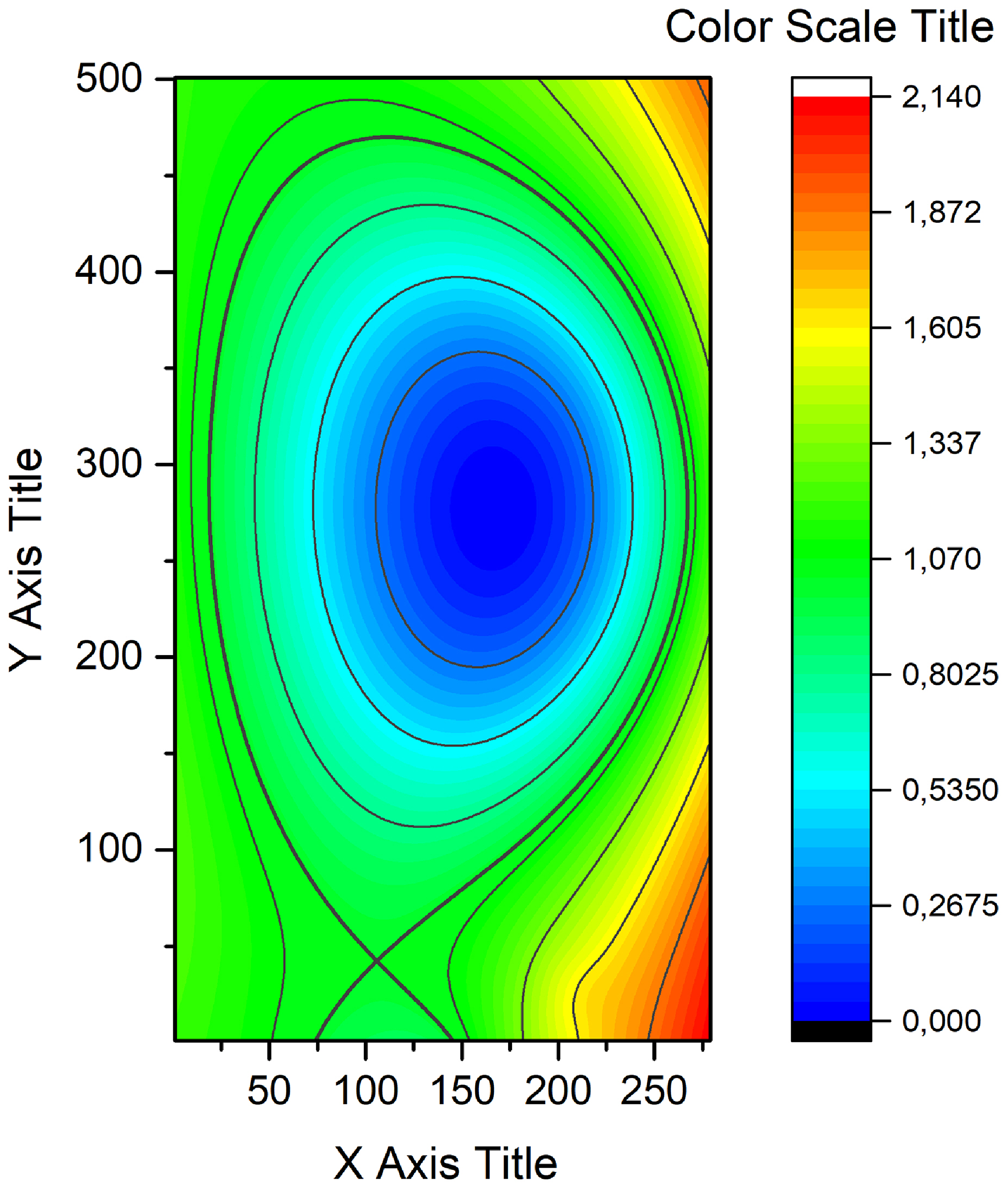
Figure 1. The magnetic surface label $\psi$
distribution in the minor cross-section of the JET tokamak. ‘Fat’ equilibrium.
$\psi$
distribution in the minor cross-section of the JET tokamak. ‘Fat’ equilibrium.
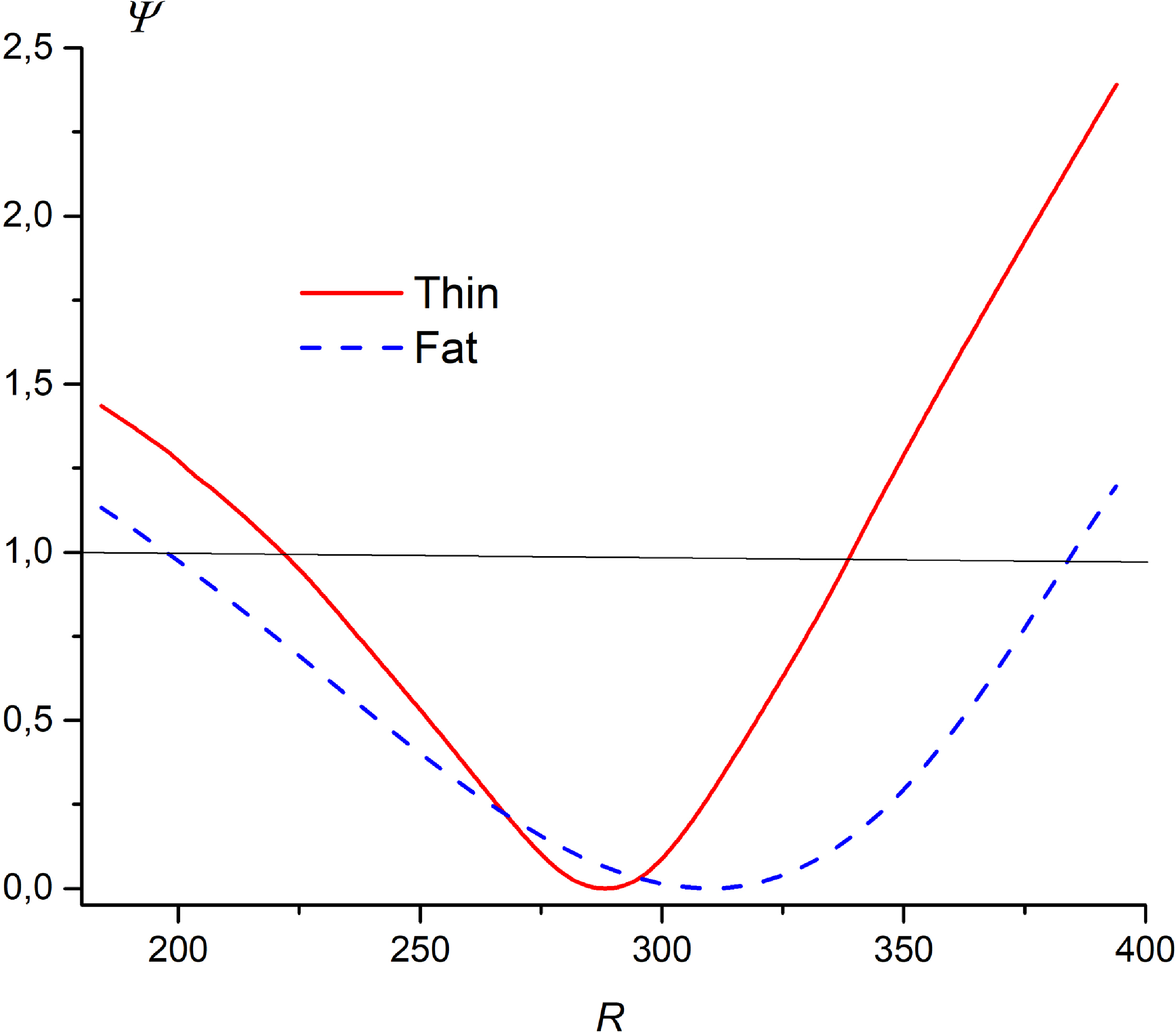
Figure 2. The magnetic flux label $\psi$
as a function of big radius R along the line that passes through the magnetic axis.
$\psi$
as a function of big radius R along the line that passes through the magnetic axis.
The realistic shape of the JET vacuum vessel was taken into account while constructing a mathematical model of the plasma density distribution in the peripheral plasma. Two distinguished magnetic configurations were used in these calculations. One of them will be referenced as ‘fat’ and the other as ‘thin’ (see figure 2).
The plasma density and temperature profiles were set as
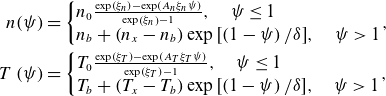 \begin{align} n\!\left(\psi \right)&=\left\{\begin{array}{l} n_{0}\frac{\exp \left(\xi _{n}\right)-\exp \left(A_{n}\xi _{n}\psi \right)}{\exp \left(\xi _{n}\right)-1},\quad \psi \leq 1\\ n_{b}+\left(n_{x}-n_{b}\right)\exp \left[\left(1-\psi \right)/\delta \right]\!,\quad \psi \gt 1 \end{array}\right.\!,\nonumber\\T\left(\psi \right)&=\left\{\begin{array}{l} T_{0}\frac{\exp \left(\xi _{T}\right)-\exp \left(A_{T}\xi _{T}\psi \right)}{\exp \left(\xi _{T}\right)-1},\quad \psi \leq 1\\ T_{b}+\left(T_{x}-T_{b}\right)\exp \left[\left(1-\psi \right)/\delta \right]\!,\quad \psi \gt 1 \end{array}\right.\!, \end{align}
where $n_{0},\,T_{0}$
are density and temperature at the axis,
$n_{0},\,T_{0}$
are density and temperature at the axis, $n_{b},\,T_{b}$
are density and temperature at the plasma boundary,
$n_{b},\,T_{b}$
are density and temperature at the plasma boundary, $A_{n},\,A_{T}$
are smoothing coefficients,
$A_{n},\,A_{T}$
are smoothing coefficients, $n_{x},\,T_{x}$
are density and temperature at the LCMS,
$n_{x},\,T_{x}$
are density and temperature at the LCMS, $\xi _{n},\,\xi _{T}$
are variable parameters (
$\xi _{n},\,\xi _{T}$
are variable parameters ( $\xi _{n}=4$
for density and
$\xi _{n}=4$
for density and $\xi _{T}=-2$
for temperature were chosen) and
$\xi _{T}=-2$
for temperature were chosen) and $\delta$
is the e-folding length outside the LCMS.
$\delta$
is the e-folding length outside the LCMS.
2.2. Ray tracing
Propagation and absorption of the SW in the JET plasma were studied using the ray-tracing code SLOWAR-T (SLOw WAve Rays in Tokamak). The SLOWAR-T code is the modified version of the code SLOWAR, described in Grekov (Reference Grekov, Albert, Turkin and Volkova2024). The verification of the dispersion relation conservation shows that it fulfills the precision of the Runge–Kutta solver, which was used in the code. The code solves the equations
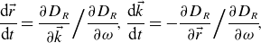 \begin{equation} \frac{\textrm{d}\vec{r}}{\textrm{d}t}=\frac{\partial D_{R}}{\partial \vec{k}}\Big/\frac{\partial D_{R}}{\partial \omega }\!,\frac{\textrm{d}\vec{k}}{\textrm{d}t}=-\frac{\partial D_{R}}{\partial \vec{r}}\Big/\frac{\partial D_{R}}{\partial \omega }\!, \end{equation}
where $\vec{k}$
is the wave vector, ω is the wave frequency, t is time,
$\vec{k}$
is the wave vector, ω is the wave frequency, t is time, $\vec{r}=(X,\enspace Y,\enspace Z)$
are the Cartesian coordinates of the ray and
$\vec{r}=(X,\enspace Y,\enspace Z)$
are the Cartesian coordinates of the ray and $D(\omega ,\vec{r},\vec{k})=0$
is the dispersion equation
$D(\omega ,\vec{r},\vec{k})=0$
is the dispersion equation
 \begin{equation} D=D_{R}+iD_{I}=\varepsilon _{1}N_{\bot }^{4}+\left[\left(\varepsilon _{3}+\varepsilon _{1}\right)\left(N_{||}^{2}-\varepsilon _{1}\right)+\varepsilon _{2}^{2}\right]N_{\bot }^{2}+\varepsilon _{3}\left[\left(N_{||}^{2}-\varepsilon _{1}\right)^{2}-\varepsilon _{2}^{2}\right]=0. \end{equation}
Here, $k_{||}=\vec{k}\cdot \vec{B}/B , \vec{B}$
is the tokamak magnetic field,
$k_{||}=\vec{k}\cdot \vec{B}/B , \vec{B}$
is the tokamak magnetic field, $N_{||}=ck_{||}/\omega , k_{\bot }=(k^{2}-k_{||}^{2})^{1/2}$
and
$N_{||}=ck_{||}/\omega , k_{\bot }=(k^{2}-k_{||}^{2})^{1/2}$
and $N_{\bot }=ck_{\bot }/\omega$
. Cylindrical coordinates
$N_{\bot }=ck_{\bot }/\omega$
. Cylindrical coordinates $(R,\enspace \phi ,\enspace Z)$
and quasi-toroidal coordinates
$(R,\enspace \phi ,\enspace Z)$
and quasi-toroidal coordinates $(r,\enspace \vartheta ,\enspace \phi )$
were also used in this investigation. Here,
$(r,\enspace \vartheta ,\enspace \phi )$
were also used in this investigation. Here, $R=\sqrt{X^{2}+Y^{2}}$
is the big radius of the torus,
$R=\sqrt{X^{2}+Y^{2}}$
is the big radius of the torus, $\phi =\textit{arctg}(Y/X)$
is the toroidal angle,
$\phi =\textit{arctg}(Y/X)$
is the toroidal angle, $\vartheta$
is the poloidal angle and
$\vartheta$
is the poloidal angle and $r$
is the minor radius of the torus.
$r$
is the minor radius of the torus.
The calculation of the dielectric tensor $\hat{\varepsilon }$
is based on the warm plasma model and resolves only electron Landau damping and fundamental ion cyclotron resonance. For
$\hat{\varepsilon }$
is based on the warm plasma model and resolves only electron Landau damping and fundamental ion cyclotron resonance. For ${\left(\omega -\omega _{c\alpha }\right)^{2}})/({2k_{||}^{2}v_{T\alpha }^{2}})\gt \gt 1$
the correction for the real part of ε
1
is negligible. For
${\left(\omega -\omega _{c\alpha }\right)^{2}})/({2k_{||}^{2}v_{T\alpha }^{2}})\gt \gt 1$
the correction for the real part of ε
1
is negligible. For ${\left((\omega -\omega _{c\alpha }\right)^{2}})/({2k_{||}^{2}v_{T\alpha }^{2}})\sim 1$
, Re(ε
1
) ∼ Im(ε
1
), D
I
∼ D
R
and the ray tracing is not applicable. The proper operator in the code terminates the calculation. Components of the tensor are defined as
${\left((\omega -\omega _{c\alpha }\right)^{2}})/({2k_{||}^{2}v_{T\alpha }^{2}})\sim 1$
, Re(ε
1
) ∼ Im(ε
1
), D
I
∼ D
R
and the ray tracing is not applicable. The proper operator in the code terminates the calculation. Components of the tensor are defined as
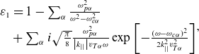 \begin{equation} \begin{array}{l} \varepsilon _{1}=1-\sum _{\alpha }\frac{\omega _{p\alpha }^{2}}{\omega ^{2}-\omega _{c\alpha }^{2}}\\ \quad+\sum _{\alpha }i\sqrt{\frac{\pi }{8}}\frac{\omega _{p\alpha }^{2}}{\left| k_{||}\right| v_{T\alpha }\omega }\exp \left[-\frac{\left(\omega -\omega _{c\alpha }\right)^{2}}{2k_{||}^{2}v_{T\alpha }^{2}}\right] \end{array}, \end{equation}
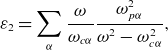 \begin{equation} \varepsilon _{2}=\sum _{\alpha }\frac{\omega }{\omega _{c\alpha }}\frac{\omega _{p\alpha }^{2}}{\omega ^{2}-\omega _{c\alpha }^{2}} ,\end{equation}
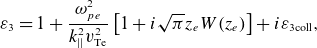 \begin{equation} \varepsilon _{3}=1+\frac{\omega _{pe}^{2}}{k_{||}^{2}v_\textrm{Te}^{2}}\left[1+i\sqrt{\pi }z_{e}W\!\left(z_{e}\right)\right]+i\varepsilon_\textrm{3coll}, \end{equation}
where mb and eb are mass and charge of b particles, b=α, e $\omega _{p\alpha }=(4\pi e^{2}n_{\alpha }/m_{\alpha })^{1/2}$
is the plasma frequency of α ions,
$\omega _{p\alpha }=(4\pi e^{2}n_{\alpha }/m_{\alpha })^{1/2}$
is the plasma frequency of α ions, $\omega _{c\alpha }=eB/cm_{\alpha }$
is the α ion cyclotron frequency,
$\omega _{c\alpha }=eB/cm_{\alpha }$
is the α ion cyclotron frequency, $v_{T\alpha }=\sqrt{T_{\alpha }/m}_{\alpha }$
is the α ion thermal velocity,
$v_{T\alpha }=\sqrt{T_{\alpha }/m}_{\alpha }$
is the α ion thermal velocity, $\omega _{pe}=(4\pi e^{2}n_{e}/m_{e})^{1/2}$
is the plasma frequency of electrons,
$\omega _{pe}=(4\pi e^{2}n_{e}/m_{e})^{1/2}$
is the plasma frequency of electrons, $v_\textrm{Te}=\sqrt{T_{e}/m}_{e}$
is the thermal velocity of electrons,
$v_\textrm{Te}=\sqrt{T_{e}/m}_{e}$
is the thermal velocity of electrons, $z_{e}=\omega /\sqrt{2}| k_{||}| v_\textrm{Te} , W(z_{e})$
is the plasma dispersion function,
$z_{e}=\omega /\sqrt{2}| k_{||}| v_\textrm{Te} , W(z_{e})$
is the plasma dispersion function, $\varepsilon_\textrm{3coll}=\omega _{pe}^{2}\nu_\textrm{eff}/\omega ^{3}$
,
$\varepsilon_\textrm{3coll}=\omega _{pe}^{2}\nu_\textrm{eff}/\omega ^{3}$
, $\nu_\textrm{eff}$
is the effective collisional frequency of electrons where
$\nu_\textrm{eff}$
is the effective collisional frequency of electrons where $\nu _{eff}=({4}/{3})\sqrt{{2\pi }/{m_{e}}}({e^{4}Z^{2} \wedge n_{e}})/({T_{e}^{3/2}})$
and Λ is the Coulomb logarithm.
$\nu _{eff}=({4}/{3})\sqrt{{2\pi }/{m_{e}}}({e^{4}Z^{2} \wedge n_{e}})/({T_{e}^{3/2}})$
and Λ is the Coulomb logarithm.
Seeing $| \varepsilon _{3}| \gt \gt | \varepsilon _{1}| ,\,| \varepsilon _{2}|$
, the solutions of equation (2.3) are
$| \varepsilon _{3}| \gt \gt | \varepsilon _{1}| ,\,| \varepsilon _{2}|$
, the solutions of equation (2.3) are
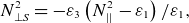 \begin{equation} N_{\bot S}^{2}=-\varepsilon _{3}\left(N_{||}^{2}-\varepsilon _{1}\right)/\varepsilon _{1}, \end{equation}
for the SW and
 \begin{equation} N_{\bot F}^{2}=\left[\left(N_{||}^{2}-\varepsilon _{1}\right)^{2}-\varepsilon _{2}^{2}\right]/\left(\varepsilon _{1}-N_{||}^{2}\right) ,\end{equation}
for the FW. Equations (2.7) and (2.8) are correct outside the conversion region, where $\varepsilon _{1}\approx N_{||}^{2}$
. Strictly speaking, ray tracing is not applicable in the regions of ray reflection and mode conversion regions. In the region of reflection of the SW from Maxwell’s equations for the
$\varepsilon _{1}\approx N_{||}^{2}$
. Strictly speaking, ray tracing is not applicable in the regions of ray reflection and mode conversion regions. In the region of reflection of the SW from Maxwell’s equations for the $E_{||}$
field of the SW the equation
$E_{||}$
field of the SW the equation $({\textrm{d}^{2}E_{||}}/{\textrm{d}\xi ^{2}})+\left({\textrm{d}k_{\bot S}^{2}}/{\textrm{d}\xi }\right)_{\xi {ref}}\left(\xi -\xi_\textrm{ref}\right)E_{||}=0$
is valid. Here,
$({\textrm{d}^{2}E_{||}}/{\textrm{d}\xi ^{2}})+\left({\textrm{d}k_{\bot S}^{2}}/{\textrm{d}\xi }\right)_{\xi {ref}}\left(\xi -\xi_\textrm{ref}\right)E_{||}=0$
is valid. Here, $\xi$
is the coordinate in the direction of the gradient of
$\xi$
is the coordinate in the direction of the gradient of $(N_{||}^{2}-\varepsilon _{1})$
. This equation is transformed to the Airy equation
$(N_{||}^{2}-\varepsilon _{1})$
. This equation is transformed to the Airy equation $({\textrm{d}^{2}E_{||}}/{\textrm{d}\varsigma ^{2}})+\varsigma E_{||}=0$
, where
$({\textrm{d}^{2}E_{||}}/{\textrm{d}\varsigma ^{2}})+\varsigma E_{||}=0$
, where $\varsigma =\left(\xi -\xi_\textrm{ref}\right)\left(({\textrm{d}k_{\bot S}^{2}}/{\textrm{d}\xi })\right)_{\xi \textrm{ref}}^{\frac{1}{3}}$
. It follows that the reflection occurs in the region
$\varsigma =\left(\xi -\xi_\textrm{ref}\right)\left(({\textrm{d}k_{\bot S}^{2}}/{\textrm{d}\xi })\right)_{\xi \textrm{ref}}^{\frac{1}{3}}$
. It follows that the reflection occurs in the region $\varsigma \sim 1$
, or
$\varsigma \sim 1$
, or $\left| \xi -\xi _{ref}\right| \approx {\unicode[Arial]{x0394}} r\sim \left(({\textrm{d}k_{\bot S}^{2}}/{\textrm{d}\xi })\right)_{\xi ref}^{-\frac{1}{3}}$
. For the selected modeling parameters,
$\left| \xi -\xi _{ref}\right| \approx {\unicode[Arial]{x0394}} r\sim \left(({\textrm{d}k_{\bot S}^{2}}/{\textrm{d}\xi })\right)_{\xi ref}^{-\frac{1}{3}}$
. For the selected modeling parameters, ${\unicode[Arial]{x0394}} r\sim 1\textrm{cm}$
. Beyond this region, the Airy function connects to the ray-tracing solutions. Thus, using the ray-tracing model only leads to inaccuracy in determining the phase only, which is of the order of
${\unicode[Arial]{x0394}} r\sim 1\textrm{cm}$
. Beyond this region, the Airy function connects to the ray-tracing solutions. Thus, using the ray-tracing model only leads to inaccuracy in determining the phase only, which is of the order of $\pi$
. Such a value of imprecision is insignificant for the present consideration. As
$\pi$
. Such a value of imprecision is insignificant for the present consideration. As $\varepsilon _{3}\lt 0$
at
$\varepsilon _{3}\lt 0$
at $n_{e}\geq 10^{7}\textrm{cm}^{-3}$
, the SW propagates in peripheral plasma only if the conditions
$n_{e}\geq 10^{7}\textrm{cm}^{-3}$
, the SW propagates in peripheral plasma only if the conditions $0\lt \varepsilon _{1}\lt N_{||}^{2}$
are fulfilled. Both of these inequalities are satisfied in hydrogen plasmas with ion cyclotron resonance frequency (ICRF) inverted minority heating (MH) or mode conversion heating (MC) regimes (Start et al. Reference Start1999; Lamalle et al. Reference Lamalle2006; Mayoral et al. Reference Mayoral2006). A key feature of these so-called inverted scenarios is that the minority ion species have a smaller charge-to-mass ratio than the majority ion species, i.e. Z
min
/A
min
$0\lt \varepsilon _{1}\lt N_{||}^{2}$
are fulfilled. Both of these inequalities are satisfied in hydrogen plasmas with ion cyclotron resonance frequency (ICRF) inverted minority heating (MH) or mode conversion heating (MC) regimes (Start et al. Reference Start1999; Lamalle et al. Reference Lamalle2006; Mayoral et al. Reference Mayoral2006). A key feature of these so-called inverted scenarios is that the minority ion species have a smaller charge-to-mass ratio than the majority ion species, i.e. Z
min
/A
min $\lt$
Z
maj
/A
maj. The wave frequency and the toroidal magnetic field are chosen so that the cyclotron resonance of the majority ions is located outside the plasma on the outer side of the torus in these experiments.
$\lt$
Z
maj
/A
maj. The wave frequency and the toroidal magnetic field are chosen so that the cyclotron resonance of the majority ions is located outside the plasma on the outer side of the torus in these experiments.
The power associated with a certain ray $Q$
is defined as
$Q$
is defined as $Q=Q_{0}e^{-{\unicode[Arial]{x0393}} }$
, where
$Q=Q_{0}e^{-{\unicode[Arial]{x0393}} }$
, where $Q_{0}$
is the initial RF power at the ray start location and
$Q_{0}$
is the initial RF power at the ray start location and ${\unicode{x1D6E4}} =\int _{0}^{t}\,\gamma \,\textrm{d}t , \gamma =-({D_{I}})/({\partial D_{R}/\partial \omega })$
. When calculating Q along the ray, electron Landau damping
${\unicode{x1D6E4}} =\int _{0}^{t}\,\gamma \,\textrm{d}t , \gamma =-({D_{I}})/({\partial D_{R}/\partial \omega })$
. When calculating Q along the ray, electron Landau damping $p_{e}$
, ion cyclotron damping
$p_{e}$
, ion cyclotron damping $p_{i\alpha }$
(α = 1, 2, 3) and collisional damping
$p_{i\alpha }$
(α = 1, 2, 3) and collisional damping $p_{col}$
were taken into account. The power dissipated along the ray
$p_{col}$
were taken into account. The power dissipated along the ray $P_\textrm{tot}$
was defined as
$P_\textrm{tot}$
was defined as $P_{tot}=Q_{0}(1-e^{-})$
. It can be represented as
$P_{tot}=Q_{0}(1-e^{-})$
. It can be represented as $P_{tot}=\int _{0}^{s}(p_\textrm{col}+p_{e}+p_{i1}+p_{i2}+p_{i3})ds$
, where
$P_{tot}=\int _{0}^{s}(p_\textrm{col}+p_{e}+p_{i1}+p_{i2}+p_{i3})ds$
, where $s=\int _{0}^{t}| \vec{v}_{g}| \textrm{d}t$
is the ray length. In what follows we assume Q
0 = 1.
$s=\int _{0}^{t}| \vec{v}_{g}| \textrm{d}t$
is the ray length. In what follows we assume Q
0 = 1.
2.3. Initial conditions
To define $\vec{k}_{0}$
for SW ray tracing, the distribution of the wave electric field E
ϕ
at the ICRF antenna must expanded into a Fourier series of poloidal (wavenumber m
0) and toroidal (wavenumber l
0) angles. It allows us to determine
$\vec{k}_{0}$
for SW ray tracing, the distribution of the wave electric field E
ϕ
at the ICRF antenna must expanded into a Fourier series of poloidal (wavenumber m
0) and toroidal (wavenumber l
0) angles. It allows us to determine $N_{\phi 0}$
as
$N_{\phi 0}$
as $N_{\phi 0}=(cl_{0})/(\omega R_{0})$
. The value of
$N_{\phi 0}=(cl_{0})/(\omega R_{0})$
. The value of $N_{z0}$
was defined as
$N_{z0}$
was defined as $N_{z0}=({cm_{0}}/{\omega \overline{a}})\cos \left[\textit{arctg}\left(Z_{0}/R_{0}\right)\right]$
, where
$N_{z0}=({cm_{0}}/{\omega \overline{a}})\cos \left[\textit{arctg}\left(Z_{0}/R_{0}\right)\right]$
, where $| m_{0}| \leq 50 , | Z_{0}| \leq 50cm$
, and
$| m_{0}| \leq 50 , | Z_{0}| \leq 50cm$
, and $\overline{a}\approx 100cm$
is a mean minor radius. Accounting for
$\overline{a}\approx 100cm$
is a mean minor radius. Accounting for $N^{2}=N_{R}^{2}+N_{\phi }^{2}+N_{z}^{2}$
and
$N^{2}=N_{R}^{2}+N_{\phi }^{2}+N_{z}^{2}$
and
 \begin{equation} N_{||}=N_{R}b_{R}+N_{\phi }b_{\phi }+N_{z}b_{z}, \end{equation}
where $(b_{R},\,b_{\phi },\,b_{z})$
are the components of the unit vector, which is parallel to the tokamak magnetic field, the initial value
$(b_{R},\,b_{\phi },\,b_{z})$
are the components of the unit vector, which is parallel to the tokamak magnetic field, the initial value $N_{R0}$
was determined from the dispersion equation (2.3). Four roots of (2.3) were found by iterations, taking
$N_{R0}$
was determined from the dispersion equation (2.3). Four roots of (2.3) were found by iterations, taking $\mathrm{Re}[W(z_{e})]$
in
$\mathrm{Re}[W(z_{e})]$
in $\varepsilon _{3}$
and assuming
$\varepsilon _{3}$
and assuming $N_{R0}=0$
in
$N_{R0}=0$
in $k_{||}$
at the first step. At subsequent iterations, the value
$k_{||}$
at the first step. At subsequent iterations, the value $N_{R0}$
from the previous iteration was substituted into
$N_{R0}$
from the previous iteration was substituted into $\varepsilon _{3}$
. Two of the roots correspond to the FW. They are complex for the chosen value of
$\varepsilon _{3}$
. Two of the roots correspond to the FW. They are complex for the chosen value of $\psi _{0}$
. The other two roots are real in the inverted scenarios and correspond to the SW . Let us call the smaller one the first root and the larger one the second root.
$\psi _{0}$
. The other two roots are real in the inverted scenarios and correspond to the SW . Let us call the smaller one the first root and the larger one the second root.
3. Features of the SW propagation and absorption in the JET tokamak
3.1. Intrinsic features of the SW. Pure hydrogen plasma
The following set of parameters has been used for consideration in this subsection: B
0 = 39 kG, n
e0
= 1 × 1013 cm−3, n
x
= 4 × 1011 cm−3, n
eb
= 1 × 1011 cm−3, n
H
/n
e
= 1.0, $T_{e0}=3\,\textrm{keV}$
, T
x
= 60 eV,
$T_{e0}=3\,\textrm{keV}$
, T
x
= 60 eV, $T_{eb}=10\,\textrm{e}V , f=\omega /2\pi =32\,\textrm{MHz}$
, the ‘fat’ equilibrium. The ray starts from a fixed point R
0 = 389 cm, Z
0 = 40 cm which in Z direction is very close to the magnetic axis.
$T_{eb}=10\,\textrm{e}V , f=\omega /2\pi =32\,\textrm{MHz}$
, the ‘fat’ equilibrium. The ray starts from a fixed point R
0 = 389 cm, Z
0 = 40 cm which in Z direction is very close to the magnetic axis.
As can be seen from figure 3(a), the SW propagates predominantly in the toroidal direction. The JET tokamak antenna system consists of two systems spaced at a toroidal angle of $\pi$
(Kaye et al. Reference Kaye, Brown, Bhatnagar, Crawley, Jacquinot, Lobel, Plancouline, Rebut, Wade and Walker1994). Therefore, the RF power emitted as SWs is uniformly distributed in the toroidal direction. In this case, the angular displacement in the poloidal direction is relatively small, of the order of
$\pi$
(Kaye et al. Reference Kaye, Brown, Bhatnagar, Crawley, Jacquinot, Lobel, Plancouline, Rebut, Wade and Walker1994). Therefore, the RF power emitted as SWs is uniformly distributed in the toroidal direction. In this case, the angular displacement in the poloidal direction is relatively small, of the order of $\pi$
/4 (see figure 3
b). This is the essential difference between SWs in the ion cyclotron frequency range and lower hybrid SWs. The latter, when propagating in tokamaks, perform many reversals in the poloidal direction (Baranov & Fedorov Reference Baranov and Fedorov1980). Also, figure 3(b) shows that SWs propagate along the periphery of the plasma and can penetrate into the divertor region.
$\pi$
/4 (see figure 3
b). This is the essential difference between SWs in the ion cyclotron frequency range and lower hybrid SWs. The latter, when propagating in tokamaks, perform many reversals in the poloidal direction (Baranov & Fedorov Reference Baranov and Fedorov1980). Also, figure 3(b) shows that SWs propagate along the periphery of the plasma and can penetrate into the divertor region.
Figure 3. The SW rays in the equatorial (a) and minor (b) cross-sections of the torus for l 0 = −40, m 0 = 2, second root – red lines and for l 0 = +40, m 0 = 2, first root – blue lines. ‘Fat’ equilibrium.
The SWs moving in the $co-\vec{B}$
direction (
$co-\vec{B}$
direction ( $N_{||}\gt 0$
, red lines in figures 3 and 4) propagate in the direction of increasing plasma density (figures 4
a and 4
b). The SWs have anomalous dispersion. The group velocity
$N_{||}\gt 0$
, red lines in figures 3 and 4) propagate in the direction of increasing plasma density (figures 4
a and 4
b). The SWs have anomalous dispersion. The group velocity $v_{g\nabla \psi }\lt 0$
together with
$v_{g\nabla \psi }\lt 0$
together with $N_{\nabla \psi }\gt 0$
at the initial part of the ray
$N_{\nabla \psi }\gt 0$
at the initial part of the ray $s\lt 550\,\textrm{cm}$
. The maximum density at which
$s\lt 550\,\textrm{cm}$
. The maximum density at which $\varepsilon _{1}=N_{||}^{2}$
or
$\varepsilon _{1}=N_{||}^{2}$
or $N_{\nabla \psi }=0$
is more than 3 × 10
12
cm−3. Since for these waves the maximum value of
$N_{\nabla \psi }=0$
is more than 3 × 10
12
cm−3. Since for these waves the maximum value of $N_{||}$
is less than 14, their Landau damping is negligible. The collisional damping (figure 4
d) is also rather small.
$N_{||}$
is less than 14, their Landau damping is negligible. The collisional damping (figure 4
d) is also rather small.
Figure 4. The flux label (a), the plasma density (b), the refractive index parallel to the magnetic field (c) and the total absorbed power (d) vs. the ray length for l 0 = −40 – red lines and for l 0 = +40 – blue lines. ‘Fat’ equilibrium.
The SWs moving in the $\textit{counter}-\vec{B}$
direction (
$\textit{counter}-\vec{B}$
direction ( $N_{||}\lt 0$
, blue lines in figures 3 and 4) propagate in the direction of the wall at first. After reflection from the wall, they slowly penetrate towards higher-density plasma. The maximum achieved density of 2.5 × 1012 cm−3 is comparable to the former case. The absolute value of
$N_{||}\lt 0$
, blue lines in figures 3 and 4) propagate in the direction of the wall at first. After reflection from the wall, they slowly penetrate towards higher-density plasma. The maximum achieved density of 2.5 × 1012 cm−3 is comparable to the former case. The absolute value of $N_{||}$
is strongly increasing at the final section of the ray. This leads to complete absorption of the SW due to Landau damping in the divertor region.
$N_{||}$
is strongly increasing at the final section of the ray. This leads to complete absorption of the SW due to Landau damping in the divertor region.
3.2. Influence of plasma density changes
In this subsection, we will study how the variation of the plasma density profile affects the propagation of the SWs. For this purpose, all parameters were fixed as in the previous subsection. At first, the parameter $\xi _{n}$
in equation (2.1) was reduced from 4 to 0. In this case, the density profile changes from very flat to parabolic.
$\xi _{n}$
in equation (2.1) was reduced from 4 to 0. In this case, the density profile changes from very flat to parabolic.
As can be seen from figure 5(a), as $\xi _{n}$
decreases, the minimum value of
$\xi _{n}$
decreases, the minimum value of $\psi$
decreases, too. This means that the SW penetrates closer and closer to the magnetic axis. However, the maximum value of the plasma density on the ray, which increases with decreasing ψ, still declines (figure 5
b). The path in the poloidal section of the torus, taken by the SW along the periphery of the plasma, increases significantly (figure 5
c). The number of revolutions of the SW around the torus also increases.
$\psi$
decreases, too. This means that the SW penetrates closer and closer to the magnetic axis. However, the maximum value of the plasma density on the ray, which increases with decreasing ψ, still declines (figure 5
b). The path in the poloidal section of the torus, taken by the SW along the periphery of the plasma, increases significantly (figure 5
c). The number of revolutions of the SW around the torus also increases.
Figure 5. The flux label (a) and the plasma density (b) vs. the ray length for $\xi _{n}=4$
(red),
$\xi _{n}=4$
(red), $\xi _{n}=2$
(green) and
$\xi _{n}=2$
(green) and $\xi _{n}=0$
(magenta), l
0 = −40. ‘Fat’ equilibrium. The SW rays in the minor cross-section (c) for the same set of parameters.
$\xi _{n}=0$
(magenta), l
0 = −40. ‘Fat’ equilibrium. The SW rays in the minor cross-section (c) for the same set of parameters.
Now the influence of the plasma density value on the magnetic axis on the wave propagation will be studied. The parameter $\xi _{n}$
is equal to 4, as before. As can be seen from figures 6(a) and 6(b), a trend similar to figure 5 is observed again. The decrease in plasma density in the center also leads to an increase in the penetration depth of the wave. And the maximum density value achievable by the SW also decreases.
$\xi _{n}$
is equal to 4, as before. As can be seen from figures 6(a) and 6(b), a trend similar to figure 5 is observed again. The decrease in plasma density in the center also leads to an increase in the penetration depth of the wave. And the maximum density value achievable by the SW also decreases.
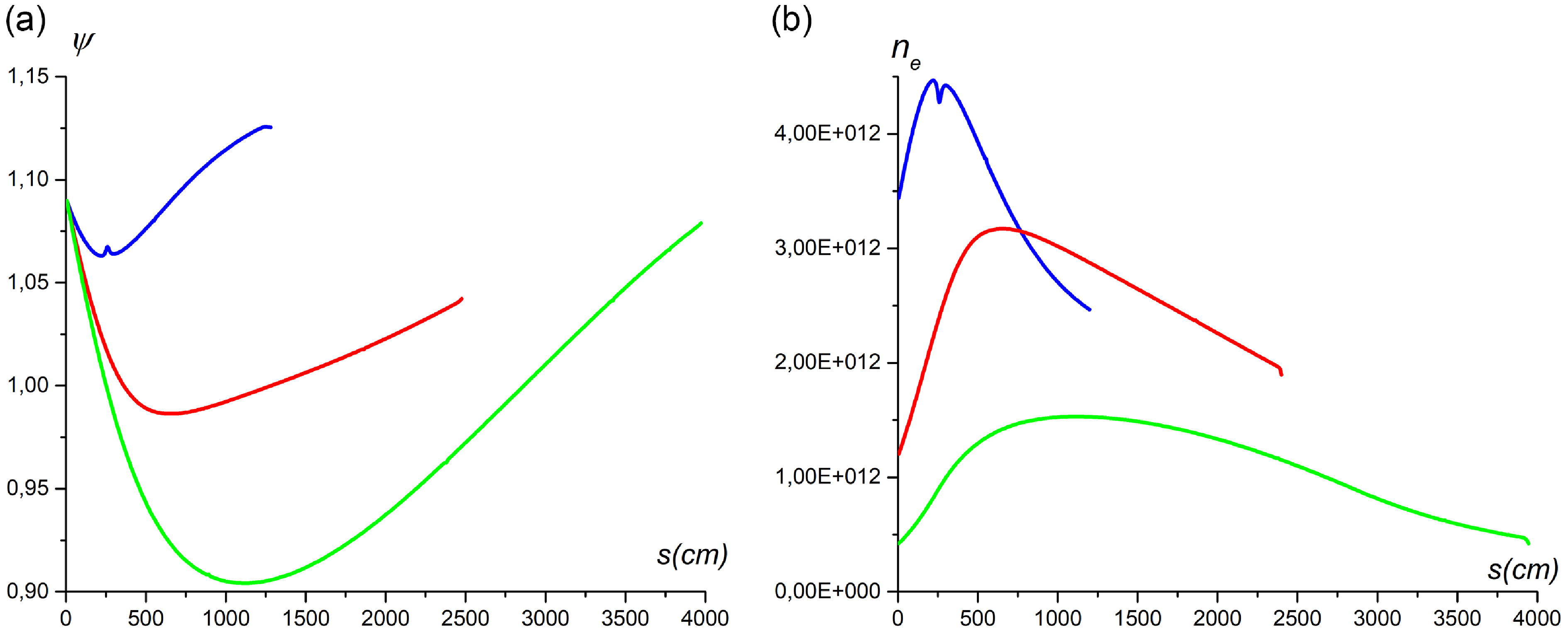
Figure 6. The flux label (a) and the plasma density (b) vs. the ray length for n e0 = 3 × 1013 cm−3 (blue), n e0 = 1 × 1013 cm−3 (red) and n e0 = 3 × 1012 cm−3 (green), l 0 = −40. ‘Fat’ equilibrium.
3.3. Effect of the initial poloidal wavenumber m0
As can be seen from figure 16 of the paper by Kaye et al. (Reference Kaye, Brown, Bhatnagar, Crawley, Jacquinot, Lobel, Plancouline, Rebut, Wade and Walker1994), the JET tokamak antenna is shielded by a screen consisting of 46 conductors. The complex structure of the electric field penetrating through such a screen can be seen in figure 2 of Lyssoivan et al. (Reference Lyssoivan2012). When such a field is expanded in a series by poloidal wavenumbers, harmonics with an initial $| m_{0}|$
of the order of 40 appear. The influence of such m
0 is shown in figure 7 for l
0 = +40.
$| m_{0}|$
of the order of 40 appear. The influence of such m
0 is shown in figure 7 for l
0 = +40.
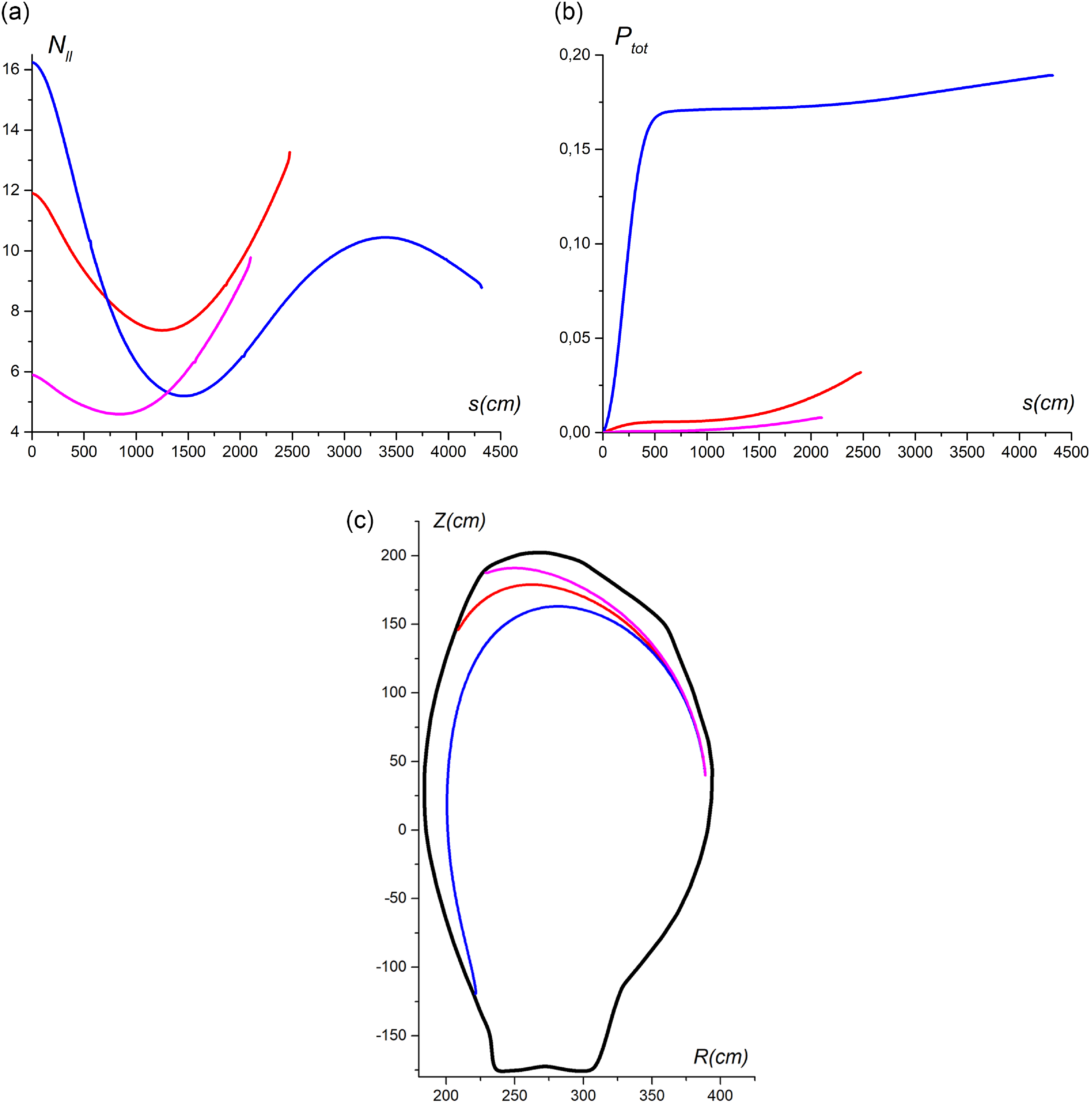
Figure 7. The refractive index parallel to the magnetic field (a) and the total absorbed power (b) vs. the ray length for m 0 = 2 – red, m 0 = −30 – blue and m 0 = +30 – magenta. The SW rays in the minor cross-section (c) for the same set of parameters. ‘Fat’ equilibrium, l 0 = −40.
As shown in figure 7(a), the initial m
0 has a strong effect on the initial $N_{||}$
. At m
0 = 50, the initial
$N_{||}$
. At m
0 = 50, the initial $N_{||}$
becomes even larger than shown in the figure. At m
0 = −50, the SW is not emitted because the initial
$N_{||}$
becomes even larger than shown in the figure. At m
0 = −50, the SW is not emitted because the initial $N_{||}$
is too small. As can be seen from figure 7(b), the collisional damping of the SW is small, of the order of several percent, in all cases. The increase in absorption for the case of m
0 = 30 is associated with the large values of
$N_{||}$
is too small. As can be seen from figure 7(b), the collisional damping of the SW is small, of the order of several percent, in all cases. The increase in absorption for the case of m
0 = 30 is associated with the large values of $N_{||}$
at the initial section of the trajectory. This leads to Landau damping of the SW on electrons. As follows from figure 7(c), the larger the initial value of m
0, the longer the path along the plasma periphery the SW travels before hitting the wall.
$N_{||}$
at the initial section of the trajectory. This leads to Landau damping of the SW on electrons. As follows from figure 7(c), the larger the initial value of m
0, the longer the path along the plasma periphery the SW travels before hitting the wall.
3.4. The SW in the ‘fat’ and ‘thin’ magnetic configurations
As can be seen from figure 2, in the ‘thin’ magnetic configuration, the region of low-density plasma between the separatrix and the wall, where the propagation of a SW is possible, is much wider than in the ‘fat’ configuration. The length of the ray in the ‘thin’ case is more than twice the length of the ray in the ‘fat’ case (figure 8 a). The first turn of the SW around the torus passes through low-density plasma. Then the plasma density along the ray path increases and reaches one third of the density on the magnetic axis (figure 8 b).
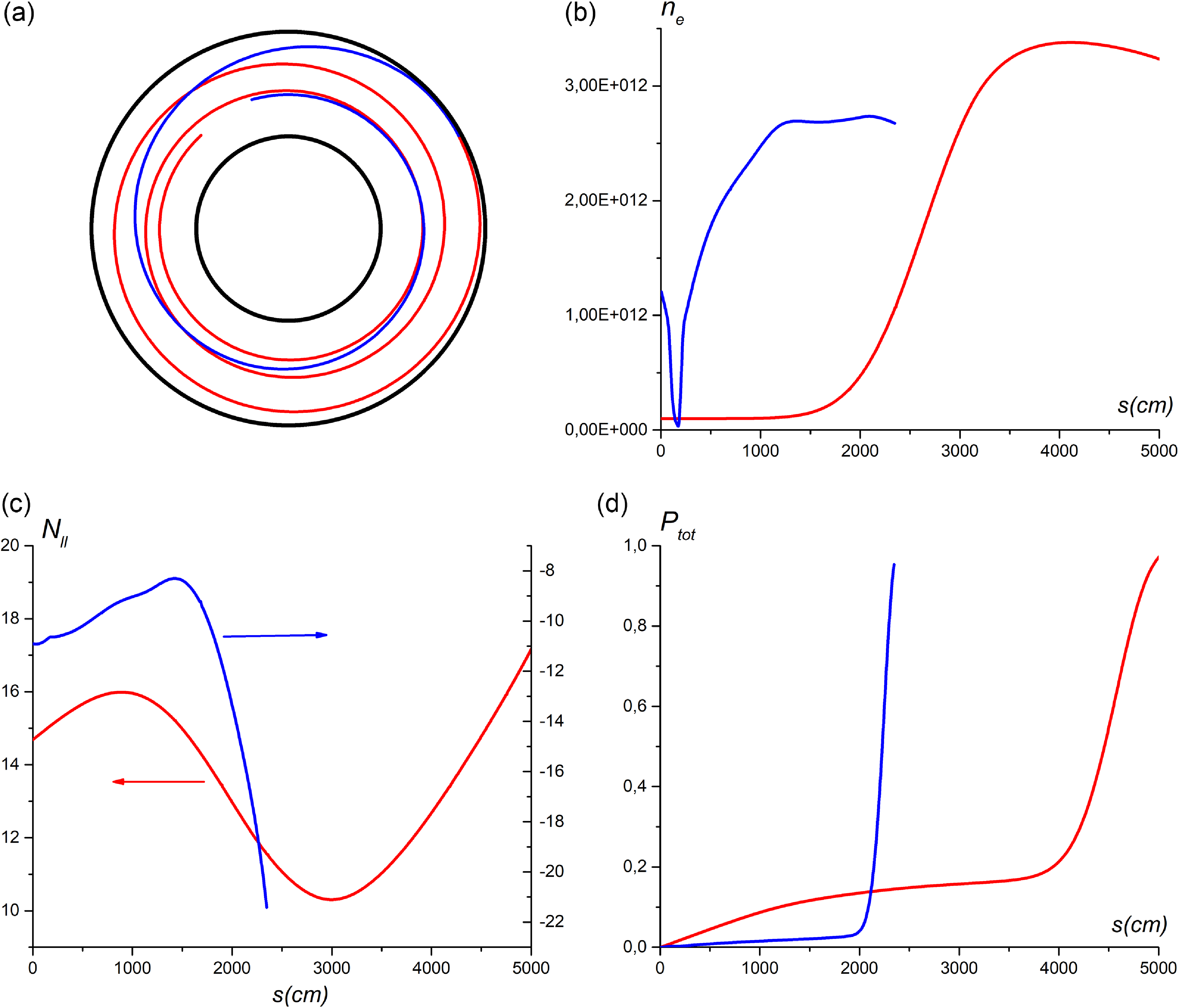
Figure 8. The SW rays in the equatorial cross-section (a), the plasma density (b), the refractive index parallel to the magnetic field (c) and the total absorbed power (d) vs. the ray length. ‘Thin’ equilibrium – red, ‘Fat’ equilibrium – blue.
Increasing $| N_{||}|$
along the ray path (figure 8
c) leads to rapid absorption of the SW due to Landau damping in both cases. In the ‘thin’ case, this is preceded by the absorption of a small, approximately 20 %, part of the RF power due to collisional damping (figure 8
d). In contrast to the ‘fat’ case, in the ‘thin’ case the propagation and absorption of the SW weakly depends on the initial value of m
0.
$| N_{||}|$
along the ray path (figure 8
c) leads to rapid absorption of the SW due to Landau damping in both cases. In the ‘thin’ case, this is preceded by the absorption of a small, approximately 20 %, part of the RF power due to collisional damping (figure 8
d). In contrast to the ‘fat’ case, in the ‘thin’ case the propagation and absorption of the SW weakly depends on the initial value of m
0.
4. The slow wave in the multi-species plasma
The § 3 set of parameters is used in this section except for B 0 = 34.5 kG, ‘thin’ equilibrium. Hydrogen (H) plasmas with minority species such as deuterium (D) and/or helium (3He) are under investigation. With this choice of parameters, the cyclotron resonance of H is located outside the plasma on the outer side of the torus. The cyclotron resonance of 3He is located at R 3He = 317 cm, and the cyclotron resonance of D is at R D = 238 cm.
The D minority affects neither the SW propagation (cf. figure 8 a and figure 9 a) nor the SW absorption (cf figure 8 d and figure 9 b).
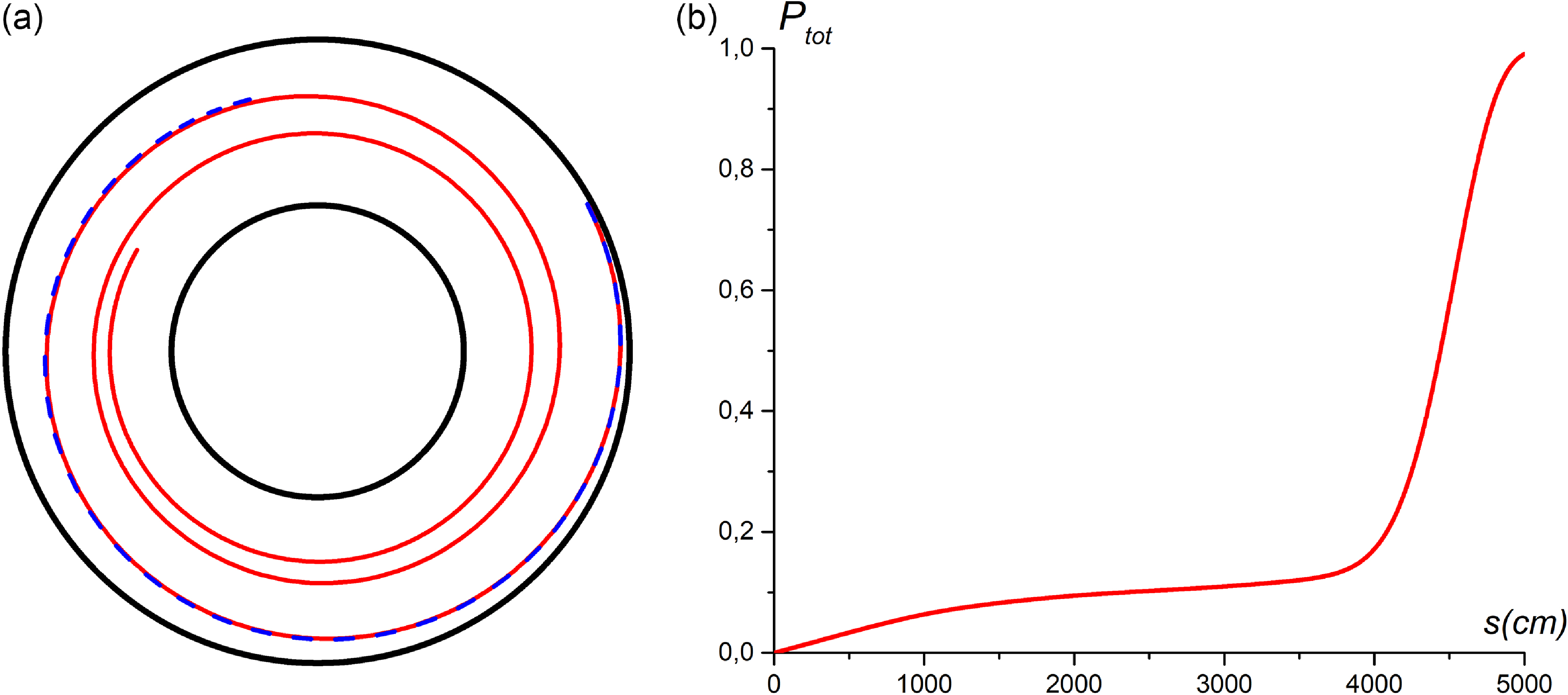
Figure 9. The SW rays in the equatorial cross-section (a); the total absorbed power vs. the ray length (b). ‘Thin’ equilibrium. Shown are D (4 %) + H (96 %) plasma – red; D (4 %) + 3He (1 %) + H (94 %) plasma – blue, dashed.
Just as in H plasma, the SW is absorbed due to collisions and Landau damping before it reaches the D–H hybrid resonance.
The 3He minority as a third ion species completely changes the SW pattern. At very low densities $n_{3He}/n_{e}\lt k_{||}\rho _{L3He}$
, the cyclotron absorption of the wave by 3He ions increases with increasing
$n_{3He}/n_{e}\lt k_{||}\rho _{L3He}$
, the cyclotron absorption of the wave by 3He ions increases with increasing $n_{3He}/n_{e}$
and at
$n_{3He}/n_{e}$
and at $n_{3He}/n_{e}\approx 0.25\,\%$
reaches 100 % (figure 10
a). Here,
$n_{3He}/n_{e}\approx 0.25\,\%$
reaches 100 % (figure 10
a). Here, $\rho _{L3He}$
is the Larmor radius of the 3He ions.
$\rho _{L3He}$
is the Larmor radius of the 3He ions.
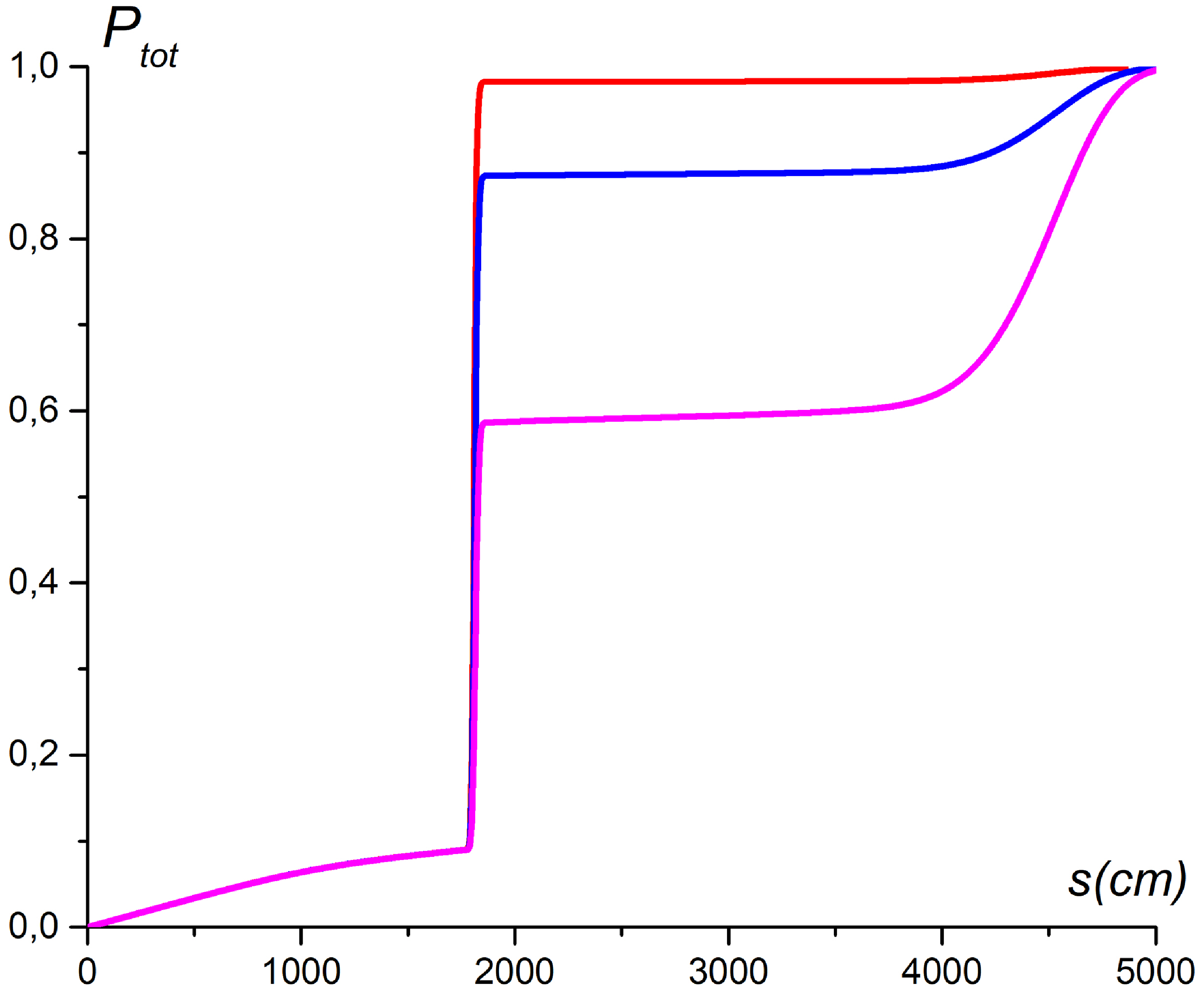
Figure 10. The total absorbed power vs. the ray length. ‘Thin’ equilibrium. Shown are D (4 %) + 3He + H plasma; 3He (0.05 %) – magenta, 3He (0.125 %) – blue; and 3He (0.25 %) – red.
These calculations are confirmed by the following estimates. The width of the cyclotron resonance ${\unicode[Arial]{x0394}} R_{c}$
is approximately equal to
${\unicode[Arial]{x0394}} R_{c}$
is approximately equal to ${\unicode[Arial]{x0394}} R_{c}\approx Ck_{||}\rho _{L3He}R$
, where C is a constant of the order of 1. The time
${\unicode[Arial]{x0394}} R_{c}\approx Ck_{||}\rho _{L3He}R$
, where C is a constant of the order of 1. The time ${\unicode[Arial]{x0394}} t_{c}$
it takes for the ray to pass through the cyclotron resonance is estimated as
${\unicode[Arial]{x0394}} t_{c}$
it takes for the ray to pass through the cyclotron resonance is estimated as ${\unicode[Arial]{x0394}} t_{c}\approx {\unicode[Arial]{x0394}} R_{c}/v_{g\nabla \psi }$
, where
${\unicode[Arial]{x0394}} t_{c}\approx {\unicode[Arial]{x0394}} R_{c}/v_{g\nabla \psi }$
, where $v_{g\nabla \psi }\sim v_{g||}\sqrt{m_{\mathrm{e}}/M_{i}}$
(Grekov et al. Reference Grekov, Albert, Turkin and Volkova2024) and
$v_{g\nabla \psi }\sim v_{g||}\sqrt{m_{\mathrm{e}}/M_{i}}$
(Grekov et al. Reference Grekov, Albert, Turkin and Volkova2024) and $v_{g||}\sim c/N_{||}$
. The optical thickness τ using these estimates is
$v_{g||}\sim c/N_{||}$
. The optical thickness τ using these estimates is $\tau =\gamma {\unicode[Arial]{x0394}} t_{c}=\frac{\mathrm{Im}\varepsilon _{1}}{\mathrm{Re}\varepsilon _{1}}\omega {\unicode[Arial]{x0394}} t_{c}\approx Cn_{3He}/n_{e}\times \omega R/v_{g\nabla \psi }$
. Setting τ = 1, we obtain
$\tau =\gamma {\unicode[Arial]{x0394}} t_{c}=\frac{\mathrm{Im}\varepsilon _{1}}{\mathrm{Re}\varepsilon _{1}}\omega {\unicode[Arial]{x0394}} t_{c}\approx Cn_{3He}/n_{e}\times \omega R/v_{g\nabla \psi }$
. Setting τ = 1, we obtain $n_{3He}/n_{e}\approx 0.2\,\%$
, which agrees well with the calculations. With a further increase in 3He density, it makes a non-negligible contribution to the dispersion of the SW. Between cyclotron resonances H and 3He, an ion–ion hybrid resonance appears. In this region, the dispersion equation (3) is not applicable, and the calculations were stopped (figure 9
a). To describe the SW in this case correctly, it is necessary to use the full kinetic dielectric tensor. Such consideration will be done elsewhere.
$n_{3He}/n_{e}\approx 0.2\,\%$
, which agrees well with the calculations. With a further increase in 3He density, it makes a non-negligible contribution to the dispersion of the SW. Between cyclotron resonances H and 3He, an ion–ion hybrid resonance appears. In this region, the dispersion equation (3) is not applicable, and the calculations were stopped (figure 9
a). To describe the SW in this case correctly, it is necessary to use the full kinetic dielectric tensor. Such consideration will be done elsewhere.
5. Conclusion
The features of the SWs’ propagation and absorption in the plasma of the JET tokamak have been investigated by ray tracing. The SWs are radiated by antennas in ICRF inverted MH or MC regimes. The SW rays propagate mainly in the toroidal direction for a distance of up to 6 × 10³
cm along and against the direction of the magnetic field. Spreading in the peripheral plasma, mainly between the LCMS and the wall, they slowly shift in the poloidal direction and can reach the divertor region. The change in equilibrium of the JET tokamak has a strong influence on both the propagation and absorption of the SWs. As the distance between the separatrix and the wall increases, the length of the rays increases. Collisional damping of the wave appears. The dependence of the propagation and absorption of the SW on the initial value of the poloidal wavenumber weakens. Cyclotron damping on H and D ions of these waves in the peripheral plasma is negligibly small. Absorption of the SWs is caused by ion–electron collisions and Landau damping. In the MH three-ion regimes, D-3He-H, the SWs are strongly damped in the cyclotron resonance of 3He ions. The cyclotron absorption of the wave by 3He ions increases with increasing $n_\textrm{3He}/n_{e}$
and at
$n_\textrm{3He}/n_{e}$
and at $n_\textrm{3He}/n_{e}\approx 0.25\,\%$
reaches 100 %. With a further increase in 3He density, it makes a non-negligible contribution to the dispersion of the SW. To describe the SW in this case correctly, it is necessary to use the full kinetic dielectric tensor. Such consideration will be done elsewhere.
$n_\textrm{3He}/n_{e}\approx 0.25\,\%$
reaches 100 %. With a further increase in 3He density, it makes a non-negligible contribution to the dispersion of the SW. To describe the SW in this case correctly, it is necessary to use the full kinetic dielectric tensor. Such consideration will be done elsewhere.
Acknowledgment
Y. Volkova is thanked for her assistance in preparing the manuscript.
Editor Peter Catto thanks the referees for their advice in evaluating this article.
Funding
This work was supported by ‘Cambridge – NFDU 2022. Individual research (development) grants for Ukrainian scientists (supported by the University of Cambridge, Great Britain)’ within the research project N 232/0022.
Declaration of interests
The authors report no conflict of interest.


 Open access