1 Introduction
Tokamaks and stellarators are magnetic confinement fusion (MCF) concepts which employ toroidal magnetic fields to confine thermonuclear plasmas. Steep gradients of density, momentum and temperature are intrinsic to most MCF concepts. For the most part, the plasma column itself is macroscopically stable, but these gradients make it prone to microscopic instabilities and non-thermal fluctuations. These micro-instabilities are well described by gyrokinetics (Catto Reference Catto1978; Antonsen & Lane Reference Antonsen and Lane1980; Frieman & Chen Reference Frieman and Chen1982). Many gyrokinetic models, algorithms, and codes have been developed and deployed over a period of decades. The first simulation algorithms used for gyrokinetics were particle-in-cell (PIC) algorithms (Lee Reference Lee1983; Kotschenreuther Reference Kotschenreuther1990; Parker & Lee Reference Parker and Lee1992; Dimits & Lee Reference Dimits and Lee1993; Denton & Kotschenreuther Reference Denton and Kotschenreuther1995; Dimits et al.
Reference Dimits, Williams, Byers and Cohen1996). Later, approaches that involved fluid moments of the gyrokinetic equation were developed. These gyrofluid (or Landau fluid) models used sophisticated (but linear) closures to model kinetic effects such as Landau damping and finite Larmor radius (FLR) effects (Hammett & Perkins Reference Hammett and Perkins1990; Hammett, Dorland & Perkins Reference Hammett, Dorland and Perkins1992; Dorland & Hammett Reference Dorland and Hammett1993; Hammett et al.
Reference Hammett, Beer, Dorland, Cowley and Smith1993; Beer & Hammett Reference Beer and Hammett1996; Snyder & Hammett Reference Snyder and Hammett2001); however, these reduced models struggled to accurately predict thermal transport levels, in part due to inaccurate zonal flow dynamics (Rosenbluth & Hinton Reference Rosenbluth and Hinton1998; Dimits et al.
Reference Dimits, Bateman, Beer, Cohen, Dorland, Hammett, Kim, Kinsey, Kotschenreuther and Kritz2000). The gyrokinetic codes that became the most widely used emerged around this time (Kotschenreuther, Rewoldt & Tang Reference Kotschenreuther, Rewoldt and Tang1995; Dorland et al.
Reference Dorland, Jenko, Kotschenreuther and Rogers2000; Jenko & Dorland Reference Jenko and Dorland2001; Candy & Waltz Reference Candy and Waltz2003). These Eulerian codes (GS2, GYRO and GENE) solve the nonlinear gyrokinetic equations on a fixed, five-dimensional mesh in phase space $(\boldsymbol{x},\boldsymbol{v})$
. Since the late 1990s, these codes have been used and cited in hundreds of papers to analyse small-scale instabilities and turbulence in tokamaks, stellarators and laboratory dipole experiments; gyrokinetic codes have also recently been repurposed for studying turbulence in astrophysical plasmas.Footnote
1
There are also many newer approaches, including semi-Lagrangian (Grandgirard et al.
Reference Grandgirard, Sarazin, Angelino, Bottino, Crouseilles, Darmet, Dif-Pradalier, Garbet, Ghendrih and Jolliet2007) and modern PIC approaches (Jolliet et al.
Reference Jolliet, Bottino, Angelino, Hatzky, Tran, McMillan, Sauter, Appert, Idomura and Villard2007). Each approach has distinct advantages, and most codes have been benchmarked extensively with one another.
$(\boldsymbol{x},\boldsymbol{v})$
. Since the late 1990s, these codes have been used and cited in hundreds of papers to analyse small-scale instabilities and turbulence in tokamaks, stellarators and laboratory dipole experiments; gyrokinetic codes have also recently been repurposed for studying turbulence in astrophysical plasmas.Footnote
1
There are also many newer approaches, including semi-Lagrangian (Grandgirard et al.
Reference Grandgirard, Sarazin, Angelino, Bottino, Crouseilles, Darmet, Dif-Pradalier, Garbet, Ghendrih and Jolliet2007) and modern PIC approaches (Jolliet et al.
Reference Jolliet, Bottino, Angelino, Hatzky, Tran, McMillan, Sauter, Appert, Idomura and Villard2007). Each approach has distinct advantages, and most codes have been benchmarked extensively with one another.
A shared weakness of these approaches is the inability to run reliably with low velocity resolution. This is despite the fact that early $\unicode[STIX]{x1D6FF}f$
PIC simulations produced accurate estimates of ion heat flux for as few as 2–4 particles per cell (Dimits et al.
Reference Dimits, Bateman, Beer, Cohen, Dorland, Hammett, Kim, Kinsey, Kotschenreuther and Kritz2000), indicating that one does not always need to resolve the fine details of the perturbed distribution function to calculate key fluctuation properties accurately. (Here, a
$\unicode[STIX]{x1D6FF}f$
PIC simulations produced accurate estimates of ion heat flux for as few as 2–4 particles per cell (Dimits et al.
Reference Dimits, Bateman, Beer, Cohen, Dorland, Hammett, Kim, Kinsey, Kotschenreuther and Kritz2000), indicating that one does not always need to resolve the fine details of the perturbed distribution function to calculate key fluctuation properties accurately. (Here, a $\unicode[STIX]{x1D6FF}f$
simulation refers to a simulation in which the full distribution function
$\unicode[STIX]{x1D6FF}f$
simulation refers to a simulation in which the full distribution function $F$
is split into a time independent background
$F$
is split into a time independent background $F_{0}$
and a perturbed distribution function
$F_{0}$
and a perturbed distribution function $\unicode[STIX]{x1D6FF}f$
that is evolved.) However, using this few particles in
$\unicode[STIX]{x1D6FF}f$
that is evolved.) However, using this few particles in $\unicode[STIX]{x1D6FF}f$
PIC is problematic due to Monte Carlo shot noise (Nevins et al.
Reference Nevins, Hammett, Dimits, Dorland and Shumaker2005; Lin et al.
Reference Lin, Holod, Chen, Diamond, Hahm and Ethier2007) and inability to resolve highly anisotropic spatial structures (Idomura, Wakatani & Tokuda Reference Idomura, Wakatani and Tokuda2000; Nevins et al.
Reference Nevins, Hammett, Dimits, Dorland and Shumaker2005). Further, the basic conservation laws are not built in, and there is no inexpensive and rigorous way to measure or control the growth of noise as the simulation progresses. Full-
$\unicode[STIX]{x1D6FF}f$
PIC is problematic due to Monte Carlo shot noise (Nevins et al.
Reference Nevins, Hammett, Dimits, Dorland and Shumaker2005; Lin et al.
Reference Lin, Holod, Chen, Diamond, Hahm and Ethier2007) and inability to resolve highly anisotropic spatial structures (Idomura, Wakatani & Tokuda Reference Idomura, Wakatani and Tokuda2000; Nevins et al.
Reference Nevins, Hammett, Dimits, Dorland and Shumaker2005). Further, the basic conservation laws are not built in, and there is no inexpensive and rigorous way to measure or control the growth of noise as the simulation progresses. Full- $f$
PIC simulations for tokamaks and stellarators, on the other hand, lack the flexibility to run with relatively constant precision at low resolution (i.e. with few particles). Conventional Eulerian gyrokinetic algorithms also lack the flexibility to run with very low velocity-space resolution while controlling discretization artefacts associated with velocity-space filamentation, although some codes such as AstroGK (Numata et al.
Reference Numata, Howes, Tatsuno, Barnes and Dorland2010) use pseudo-spectral grids to increase the accuracy of integrals.
$f$
PIC simulations for tokamaks and stellarators, on the other hand, lack the flexibility to run with relatively constant precision at low resolution (i.e. with few particles). Conventional Eulerian gyrokinetic algorithms also lack the flexibility to run with very low velocity-space resolution while controlling discretization artefacts associated with velocity-space filamentation, although some codes such as AstroGK (Numata et al.
Reference Numata, Howes, Tatsuno, Barnes and Dorland2010) use pseudo-spectral grids to increase the accuracy of integrals.
In this work we present a pseudo-spectral velocity formulation of gyrokinetics. Unlike the Eulerian algorithms described above that discretize velocity space on a mesh, our approach projects the gyrokinetic equation onto a velocity basis composed of Laguerre and Hermite polynomials.Footnote 2 Projecting the distribution function onto this basis produces fluid-like quantities, which correspond to density, parallel momentum, etc. The result is a formulation that is equivalent to a generalized gyrofluid system with arbitrarily many moments, which at high velocity-space resolution corresponds directly to conventional gyrokinetic Eulerian models. A key advantage of our approach is the flexibility to use very low velocity-space resolution within the same framework, where the system corresponds precisely to the well-established gyrofluid models described above. Further, since our approach produces a system of fluid-quantity conservation laws, one can maintain fundamental properties like number, momentum and energy conservation, even at very low resolution. Any inaccuracy from using low resolution can be isolated to the shortcomings of the closure assumptions used. For example, truncating the system appropriately reproduces the reduced double-adiabatic equations, which conserve number, momentum and the first and second adiabatic invariants. Importantly, since the worst case scenario is the level of accuracy of the original gyrofluid models (which used only 6 moments), our model should be able to obtain fairly precise estimates of most quantities of interest at resolutions only modestly higher than that of the original gyrofluid models. We also present a model collision operator which has a particularly sparse representation in the Laguerre–Hermite basis. This collision operator maintains conservation laws and the H theorem.
The particular application we target is the modelling of MCF turbulence in the context of whole-device modelling (WDM). The WDM idea is to simulate the full operation of a tokamak or stellarator, from the currents in the external magnets to heating systems, to turbulence, etc. with the run-time flexibility to use a range of models for any given process in any given calculation, depending on the fidelity required for that process for that simulation run. Our model can run at relatively low velocity resolution as an inexpensive WDM module, producing a significant performance advantage over other approaches, or at high resolution at costs comparable to the state of the art. Thus, a Laguerre–Hermite pseudo-spectral gyrokinetic module for WDM applications promises good fidelity at modest cost, together with straightforward validation at high resolution.
This paper is organized as follows: in § 2, we introduce the gyrokinetic equation, which is the starting point of our approach. In § 3, we project this equation onto the Laguerre–Hermite basis, discussing details of our model collision operator in § 3.5. Section 4 discusses free energy and its conservation in the context of this formulation. We present linear results of our model in § 5, and discuss conclusions and future work in § 6.
2 Gyrokinetic description of dynamics
The literature of gyrokinetics and gyrokinetic turbulence is vast and mature. Our notation and philosophy follow four particular references: Antonsen & Lane (Reference Antonsen and Lane1980), Frieman & Chen (Reference Frieman and Chen1982), Barnes et al. (Reference Barnes, Abel, Dorland, Görler, Hammett and Jenko2010) and Abel et al. (Reference Abel, Plunk, Wang, Barnes, Cowley, Dorland and Schekochihin2013). Detailed discussions that appear in these papers are not repeated here unless necessary. In the context of the latter, this report describes a potentially useful representation of the nonlinear $\unicode[STIX]{x1D6FF}f$
gyrokinetic equation [equation (108) of Abel et al. (Reference Abel, Plunk, Wang, Barnes, Cowley, Dorland and Schekochihin2013)] in the absence of strong equilibrium flows and in the absence of electromagnetic fluctuations. Our immediate goal is to derive a model appropriate for radially local, flux-tube simulations, such as would be used to describe the turbulent fluxes through a given flux surface of a global WDM simulation. Generalization of our final equations for radially global applications would require the derivation of physically plausible, radially non-periodic, gyrokinetic boundary conditions and a more nuanced treatment of short wavelength finite Larmor radius effects. Inclusion of electromagnetic fluctuations challenges the kinds of closure models we favour, even in the radially local, flux-tube limit (Snyder & Hammett Reference Snyder and Hammett2001). Generalizing the model to include strong flows, on the other hand, is straightforward.
$\unicode[STIX]{x1D6FF}f$
gyrokinetic equation [equation (108) of Abel et al. (Reference Abel, Plunk, Wang, Barnes, Cowley, Dorland and Schekochihin2013)] in the absence of strong equilibrium flows and in the absence of electromagnetic fluctuations. Our immediate goal is to derive a model appropriate for radially local, flux-tube simulations, such as would be used to describe the turbulent fluxes through a given flux surface of a global WDM simulation. Generalization of our final equations for radially global applications would require the derivation of physically plausible, radially non-periodic, gyrokinetic boundary conditions and a more nuanced treatment of short wavelength finite Larmor radius effects. Inclusion of electromagnetic fluctuations challenges the kinds of closure models we favour, even in the radially local, flux-tube limit (Snyder & Hammett Reference Snyder and Hammett2001). Generalizing the model to include strong flows, on the other hand, is straightforward.
We begin with a non-dimensional, normalized form of the electrostatic gyrokinetic equation:
 $$\begin{eqnarray}\frac{\unicode[STIX]{x2202}g_{s}}{\unicode[STIX]{x2202}t}+\left[v_{ts}v_{\Vert }\hat{\boldsymbol{b}}+\langle \boldsymbol{v}_{E}\rangle _{\boldsymbol{R}}+\frac{\unicode[STIX]{x1D70F}_{s}}{Z_{s}}\boldsymbol{v}_{d}\right]\boldsymbol{\cdot }\unicode[STIX]{x1D735}h_{s}+\langle \boldsymbol{v}_{E}\rangle _{\boldsymbol{R}}\boldsymbol{\cdot }\unicode[STIX]{x1D735}F_{Ms}-v_{ts}\unicode[STIX]{x1D707}(\hat{\boldsymbol{b}}\boldsymbol{\cdot }\unicode[STIX]{x1D735}B)\frac{\unicode[STIX]{x2202}h_{s}}{\unicode[STIX]{x2202}v_{\Vert }}=C(h_{s}).\end{eqnarray}$$
This equation describes the evolution of the fluctuating gyrokinetic distribution function $g_{s}=g_{s}(\boldsymbol{R},v_{\Vert },\unicode[STIX]{x1D707},t)$
for a particular species
$g_{s}=g_{s}(\boldsymbol{R},v_{\Vert },\unicode[STIX]{x1D707},t)$
for a particular species $s$
. All quantities in the above equation (e.g.
$s$
. All quantities in the above equation (e.g. $h,g,\boldsymbol{v}_{E},v_{\Vert },\unicode[STIX]{x1D707},t$
, etc.) have been non-dimensionalized, with the specific normalizations explained in appendix A. The total distribution function,
$h,g,\boldsymbol{v}_{E},v_{\Vert },\unicode[STIX]{x1D707},t$
, etc.) have been non-dimensionalized, with the specific normalizations explained in appendix A. The total distribution function, $F_{s}=F_{0s}+\unicode[STIX]{x1D6FF}f_{s}=F_{Ms}(1-Z_{s}\unicode[STIX]{x1D6F7}/\unicode[STIX]{x1D70F}_{s})+h_{s}$
is a Maxwellian with a small Boltzmann component [
$F_{s}=F_{0s}+\unicode[STIX]{x1D6FF}f_{s}=F_{Ms}(1-Z_{s}\unicode[STIX]{x1D6F7}/\unicode[STIX]{x1D70F}_{s})+h_{s}$
is a Maxwellian with a small Boltzmann component [ $\propto \unicode[STIX]{x1D6F7}(\boldsymbol{r},t)$
, the electrostatic potential] and a general perturbation,
$\propto \unicode[STIX]{x1D6F7}(\boldsymbol{r},t)$
, the electrostatic potential] and a general perturbation, $h_{s}(\boldsymbol{R},v_{\Vert },\unicode[STIX]{x1D707},t)$
. The total gyroaveraged distribution function,
$h_{s}(\boldsymbol{R},v_{\Vert },\unicode[STIX]{x1D707},t)$
. The total gyroaveraged distribution function, $\langle F_{s}\rangle _{\boldsymbol{R}}=F_{0s}+g_{s}$
, with
$\langle F_{s}\rangle _{\boldsymbol{R}}=F_{0s}+g_{s}$
, with $g_{s}=h_{s}-(Z_{s}/\unicode[STIX]{x1D70F}_{s})\langle \unicode[STIX]{x1D6F7}\rangle _{\boldsymbol{R}}F_{Ms}$
, describes the probability of finding a particle of species
$g_{s}=h_{s}-(Z_{s}/\unicode[STIX]{x1D70F}_{s})\langle \unicode[STIX]{x1D6F7}\rangle _{\boldsymbol{R}}F_{Ms}$
, describes the probability of finding a particle of species $s$
with guiding centre (or gyrocentre) position
$s$
with guiding centre (or gyrocentre) position $\boldsymbol{R}$
, velocity parallel to the magnetic field
$\boldsymbol{R}$
, velocity parallel to the magnetic field $v_{\Vert }$
, and magnetic moment
$v_{\Vert }$
, and magnetic moment $\unicode[STIX]{x1D707}=v_{\bot }^{2}/2B$
, where
$\unicode[STIX]{x1D707}=v_{\bot }^{2}/2B$
, where $v_{\bot }$
is the speed in the plane perpendicular to the magnetic field. The electrostatic potential
$v_{\bot }$
is the speed in the plane perpendicular to the magnetic field. The electrostatic potential $\unicode[STIX]{x1D6F7}=\unicode[STIX]{x1D6F7}(\boldsymbol{r},t)$
is a function of particle position
$\unicode[STIX]{x1D6F7}=\unicode[STIX]{x1D6F7}(\boldsymbol{r},t)$
is a function of particle position $\boldsymbol{r}$
, where
$\boldsymbol{r}$
, where $\boldsymbol{r}=\boldsymbol{R}+\unicode[STIX]{x1D746}$
so that
$\boldsymbol{r}=\boldsymbol{R}+\unicode[STIX]{x1D746}$
so that $\unicode[STIX]{x1D746}$
is the gyroradius vector that rotates at the gyrofrequency
$\unicode[STIX]{x1D746}$
is the gyroradius vector that rotates at the gyrofrequency $\unicode[STIX]{x1D6FA}$
and points from the gyrocentre (at
$\unicode[STIX]{x1D6FA}$
and points from the gyrocentre (at $\boldsymbol{R}$
) to the particle (at
$\boldsymbol{R}$
) to the particle (at $\boldsymbol{r}$
). The equilibrium magnetic field
$\boldsymbol{r}$
). The equilibrium magnetic field $\boldsymbol{B}$
has magnitude
$\boldsymbol{B}$
has magnitude $B$
and direction
$B$
and direction $\hat{\boldsymbol{b}}=\boldsymbol{B}/B$
.
$\hat{\boldsymbol{b}}=\boldsymbol{B}/B$
.
The equilibrium distribution function is a Maxwellian (which we take to have no flows),
 $$\begin{eqnarray}F_{0s}=F_{Ms}=\frac{n_{s}}{(2\unicode[STIX]{x03C0}v_{ts}^{2})^{3/2}}\text{e}^{-v_{\Vert }^{2}/2-\unicode[STIX]{x1D707}B},\end{eqnarray}$$
and the fluctuating gyroaveraged distribution function satisfies $g\ll F_{M}$
. We also have the following dimensionless species parameters: equilibrium density
$g\ll F_{M}$
. We also have the following dimensionless species parameters: equilibrium density $n_{s}(\unicode[STIX]{x1D6F9})$
, equilibrium temperature
$n_{s}(\unicode[STIX]{x1D6F9})$
, equilibrium temperature $\unicode[STIX]{x1D70F}_{s}(\unicode[STIX]{x1D6F9})$
, mass
$\unicode[STIX]{x1D70F}_{s}(\unicode[STIX]{x1D6F9})$
, mass $m_{s}$
, charge
$m_{s}$
, charge $Z_{s}$
and thermal velocity
$Z_{s}$
and thermal velocity $v_{ts}=\sqrt{\unicode[STIX]{x1D70F}_{s}/m_{s}}$
. Here
$v_{ts}=\sqrt{\unicode[STIX]{x1D70F}_{s}/m_{s}}$
. Here $\unicode[STIX]{x1D6F9}=\langle \unicode[STIX]{x1D6F9}\rangle _{\boldsymbol{R}}=\langle \unicode[STIX]{x1D6F9}\rangle _{\boldsymbol{r}}$
is the poloidal flux, which labels flux surfaces and effectively serves as a radial coordinate. In flux-tube geometry, all equilibrium quantities such as
$\unicode[STIX]{x1D6F9}=\langle \unicode[STIX]{x1D6F9}\rangle _{\boldsymbol{R}}=\langle \unicode[STIX]{x1D6F9}\rangle _{\boldsymbol{r}}$
is the poloidal flux, which labels flux surfaces and effectively serves as a radial coordinate. In flux-tube geometry, all equilibrium quantities such as $n_{s}$
,
$n_{s}$
, $\unicode[STIX]{x1D70F}_{s}$
,
$\unicode[STIX]{x1D70F}_{s}$
, $B$
(and therefore
$B$
(and therefore $\unicode[STIX]{x1D70C}$
) are assumed to be constant in each radially local flux-tube domain.
$\unicode[STIX]{x1D70C}$
) are assumed to be constant in each radially local flux-tube domain.
The notation $\langle \cdots \rangle _{\boldsymbol{R}}$
denotes a gyroaverage taken at constant
$\langle \cdots \rangle _{\boldsymbol{R}}$
denotes a gyroaverage taken at constant $\boldsymbol{R}$
.Footnote
3
The gyroaveraged
$\boldsymbol{R}$
.Footnote
3
The gyroaveraged $\boldsymbol{E}\times \boldsymbol{B}$
velocity is
$\boldsymbol{E}\times \boldsymbol{B}$
velocity is $\langle \boldsymbol{v}_{E}\rangle _{\boldsymbol{R}}=\hat{\boldsymbol{b}}\times \unicode[STIX]{x1D735}\langle \unicode[STIX]{x1D6F7}\rangle _{\boldsymbol{R}}$
, the magnetic drift velocity is
$\langle \boldsymbol{v}_{E}\rangle _{\boldsymbol{R}}=\hat{\boldsymbol{b}}\times \unicode[STIX]{x1D735}\langle \unicode[STIX]{x1D6F7}\rangle _{\boldsymbol{R}}$
, the magnetic drift velocity is $\boldsymbol{v}_{d}=(v_{\Vert }^{2}+\unicode[STIX]{x1D707}B)\hat{\boldsymbol{b}}\times \unicode[STIX]{x1D735}B/B^{2}$
, and we take
$\boldsymbol{v}_{d}=(v_{\Vert }^{2}+\unicode[STIX]{x1D707}B)\hat{\boldsymbol{b}}\times \unicode[STIX]{x1D735}B/B^{2}$
, and we take $\unicode[STIX]{x1D735}\equiv \unicode[STIX]{x2202}/\unicode[STIX]{x2202}\boldsymbol{R}$
throughout. The collision operator, which we define in § 3.5, is denoted by
$\unicode[STIX]{x1D735}\equiv \unicode[STIX]{x2202}/\unicode[STIX]{x2202}\boldsymbol{R}$
throughout. The collision operator, which we define in § 3.5, is denoted by $C(h)$
.Footnote
4
Finally, the potential is determined by the quasineutrality equation, which we also write in terms of
$C(h)$
.Footnote
4
Finally, the potential is determined by the quasineutrality equation, which we also write in terms of $h$
:
$h$
:
 $$\begin{eqnarray}\mathop{\sum }_{s}Z_{s}n_{s}\int \text{d}^{3}\boldsymbol{v}\,\langle h_{s}\rangle _{\boldsymbol{r}}=\mathop{\sum }_{s}\frac{n_{s}Z_{s}^{2}}{\unicode[STIX]{x1D70F}_{s}}\unicode[STIX]{x1D6F7}.\end{eqnarray}$$
In the limit of a single hydrogenic ion species with Boltzmann electrons, this reduces to
 $$\begin{eqnarray}\int \text{d}^{3}\boldsymbol{v}\,\langle h\rangle _{\boldsymbol{ r}}=\unicode[STIX]{x1D70F}_{e}^{-1}[\unicode[STIX]{x1D6F7}-\langle \langle \unicode[STIX]{x1D6F7}\rangle \rangle ]+\unicode[STIX]{x1D6F7},\end{eqnarray}$$
where $\unicode[STIX]{x1D70F}_{e}=T_{e}/T_{i}$
in this limit of
$\unicode[STIX]{x1D70F}_{e}=T_{e}/T_{i}$
in this limit of $T_{i}=T_{\text{ref}}$
. (Note that several authors choose the reciprocal definition for
$T_{i}=T_{\text{ref}}$
. (Note that several authors choose the reciprocal definition for $\unicode[STIX]{x1D70F}_{e}$
.) The flux-surface average is denoted by
$\unicode[STIX]{x1D70F}_{e}$
.) The flux-surface average is denoted by $\langle \langle \cdots \rangle \rangle$
. This term comes from the standard correction for Boltzmann electrons (Dorland & Hammett Reference Dorland and Hammett1993), which ensures that the flux-surface-averaged electron density perturbation vanishes.
$\langle \langle \cdots \rangle \rangle$
. This term comes from the standard correction for Boltzmann electrons (Dorland & Hammett Reference Dorland and Hammett1993), which ensures that the flux-surface-averaged electron density perturbation vanishes.
Equations (2.1) and (2.4) describe self-consistent electrostatic gyrokinetic dynamics in field-line-following coordinates, including magnetically trapped particles and as yet unspecified collisional physics. These equations can be solved in general geometry (tokamak and stellarator) to find the instabilities, fluctuation spectra and turbulent fluxes of particles and energy. Landau damping, trapped particle effects, and other ‘kinetic’ phenomena are described by this comprehensive approach.
3 Laguerre–Hermite pseudo-spectral formulation
Our basic approach is to project the velocity dependence of the fluctuating distribution functions $h$
and
$h$
and $g$
onto orthonormal polynomials. The result is a spectral representationFootnote
5
within which the amplitudes of the polynomial basis functions, which can be interpreted as fluid moments,Footnote
6
become the dynamical variables. Thus instead of keeping track of
$g$
onto orthonormal polynomials. The result is a spectral representationFootnote
5
within which the amplitudes of the polynomial basis functions, which can be interpreted as fluid moments,Footnote
6
become the dynamical variables. Thus instead of keeping track of $g(v_{\Vert },\unicode[STIX]{x1D707}B)$
with a finite-difference algorithm on a discretized
$g(v_{\Vert },\unicode[STIX]{x1D707}B)$
with a finite-difference algorithm on a discretized $(v_{\Vert },\unicode[STIX]{x1D707}B)$
grid, we evolve coupled fluid-like quantities, such as density, parallel momentum, etc., which emerge from the projection. Specifically, we project onto Hermite polynomials in the
$(v_{\Vert },\unicode[STIX]{x1D707}B)$
grid, we evolve coupled fluid-like quantities, such as density, parallel momentum, etc., which emerge from the projection. Specifically, we project onto Hermite polynomials in the $v_{\Vert }$
coordinate and Laguerre polynomials in the
$v_{\Vert }$
coordinate and Laguerre polynomials in the $\unicode[STIX]{x1D707}B$
coordinate. We choose this basis in part because the resulting system is identical at low resolution to the gyrofluid models of Dorland & Hammett (Reference Dorland and Hammett1993), and Beer & Hammett (Reference Beer and Hammett1996). The Laguerre and Hermite polynomials are also orthogonal with respect to a Maxwellian. Further, the Laguerre and Hermite polynomials are eigenfunctions of our model collision operator, described in § 3.5.
$\unicode[STIX]{x1D707}B$
coordinate. We choose this basis in part because the resulting system is identical at low resolution to the gyrofluid models of Dorland & Hammett (Reference Dorland and Hammett1993), and Beer & Hammett (Reference Beer and Hammett1996). The Laguerre and Hermite polynomials are also orthogonal with respect to a Maxwellian. Further, the Laguerre and Hermite polynomials are eigenfunctions of our model collision operator, described in § 3.5.
At fixed accuracy, pseudo-spectral algorithms are very efficient and thus produce a small footprint in device memory (Boyd Reference Boyd2001). This makes it possible to move a well-resolved gyrokinetic simulation of ion temperature gradient-driven tokamak turbulence from hundreds or thousands of cores on a massively parallel supercomputer to a single graphics processor (GPU). Additionally, the regular memory access patterns of a pseudo-spectral formulation are well matched to the advantages of the GPU architecture (or any comparably high-performance vector hardware).
3.1 Pseudo-spectral in phase space
Our approach is perhaps best understood by analogy with pseudo-spectral Fourier methods. Consider a Fourier decomposition for the spatial coordinates in the gyrokinetic equation. By using field-line-following coordinates to avoid irregular domains (Beer, Cowley & Hammett Reference Beer, Cowley and Hammett1995), Fourier techniques can be readily applied; periodic (and otherwise appropriate) domains are guaranteed by the asymptotics of the problem (Abel et al.
Reference Abel, Plunk, Wang, Barnes, Cowley, Dorland and Schekochihin2013). Such a Fourier decomposition has the advantage of allowing spectrally accurate evaluation of the derivatives because the spatial derivative has Fourier harmonics as its eigenfunctions [ $\text{d}/\text{d}x\exp (\text{i}kx)=\text{i}k\exp (\text{i}kx)$
]. Conversely, achieving spectral accuracy in evaluating derivatives with a finite-difference, real-space representation on an
$\text{d}/\text{d}x\exp (\text{i}kx)=\text{i}k\exp (\text{i}kx)$
]. Conversely, achieving spectral accuracy in evaluating derivatives with a finite-difference, real-space representation on an $n$
-point grid requires the use of
$n$
-point grid requires the use of $n$
-point stencils, which is expensive. There are costs, of course, that reduce the advantages of a Fourier representation. Nonlinearity, in particular, necessitates the evaluation of convolutions in a strict Fourier basis: quadratic nonlinearities introduce spectral convolutions with
$n$
-point stencils, which is expensive. There are costs, of course, that reduce the advantages of a Fourier representation. Nonlinearity, in particular, necessitates the evaluation of convolutions in a strict Fourier basis: quadratic nonlinearities introduce spectral convolutions with $O(n^{2})$
terms. Pseudo-spectral algorithms reduce this operator count to
$O(n^{2})$
terms. Pseudo-spectral algorithms reduce this operator count to $O(n\log n)$
by using fast discrete transforms to evaluate the nonlinear terms in real space, without the loss of spectral accuracy.
$O(n\log n)$
by using fast discrete transforms to evaluate the nonlinear terms in real space, without the loss of spectral accuracy.
Our new approach takes this a step further by using pseudo-spectral methods not only in configuration space but also in velocity space. Instead of working with $f(\boldsymbol{R},\boldsymbol{v})$
, we Fourier transform in the spatial coordinate
$f(\boldsymbol{R},\boldsymbol{v})$
, we Fourier transform in the spatial coordinate $\boldsymbol{R}$
and Laguerre–Hermite transform in the velocity coordinate
$\boldsymbol{R}$
and Laguerre–Hermite transform in the velocity coordinate $\boldsymbol{v}$
to develop spectral equations governing the evolution of
$\boldsymbol{v}$
to develop spectral equations governing the evolution of $f(\boldsymbol{k},\boldsymbol{p})$
. Here,
$f(\boldsymbol{k},\boldsymbol{p})$
. Here, $\boldsymbol{k}$
is the usual Fourier wavenumber, and
$\boldsymbol{k}$
is the usual Fourier wavenumber, and $\boldsymbol{p}=(\ell ,m)$
is the ‘wavenumber’ in the Laguerre–Hermite dual to velocity space. The advantages of the Fourier decomposition discussed in the previous paragraph apply to velocity space as well. Just as a Fourier decomposition in space has the advantage of spectrally accurate evaluation of spatial derivatives, our Laguerre–Hermite spectral velocity decomposition allows spectrally accurate evaluation of the velocity derivatives that appear in (2.1) and in the collision operator. Nonlinearities may be evaluated pseudo-spectrally relatively inexpensively in
$\boldsymbol{p}=(\ell ,m)$
is the ‘wavenumber’ in the Laguerre–Hermite dual to velocity space. The advantages of the Fourier decomposition discussed in the previous paragraph apply to velocity space as well. Just as a Fourier decomposition in space has the advantage of spectrally accurate evaluation of spatial derivatives, our Laguerre–Hermite spectral velocity decomposition allows spectrally accurate evaluation of the velocity derivatives that appear in (2.1) and in the collision operator. Nonlinearities may be evaluated pseudo-spectrally relatively inexpensively in $(\boldsymbol{R},\boldsymbol{v})$
space with the use of efficient transforms and appropriately chosen grids. We expect this fully pseudo-spectral formulation of gyrokinetics to be a useful addition to the community toolbox.
$(\boldsymbol{R},\boldsymbol{v})$
space with the use of efficient transforms and appropriately chosen grids. We expect this fully pseudo-spectral formulation of gyrokinetics to be a useful addition to the community toolbox.
There are disadvantages to our approach, too. In addition to derivatives in velocity space, there are multiplications by velocity in the gyrokinetic equation. The canonical example is the free streaming of particles along the magnetic field $({\sim}v_{\Vert }\,\text{d}/\text{d}z)$
, which introduces a term like
$({\sim}v_{\Vert }\,\text{d}/\text{d}z)$
, which introduces a term like $\text{i}k_{z}v_{\Vert }$
to the fluctuation equations which describe a general fluctuation
$\text{i}k_{z}v_{\Vert }$
to the fluctuation equations which describe a general fluctuation $\unicode[STIX]{x1D6FF}f\,(\boldsymbol{k},\boldsymbol{v})$
. In
$\unicode[STIX]{x1D6FF}f\,(\boldsymbol{k},\boldsymbol{v})$
. In $(\boldsymbol{R},v)$
space, a term like this can be evaluated with a finite-difference scheme (Kotschenreuther et al.
Reference Kotschenreuther, Rewoldt and Tang1995; Jenko et al.
Reference Jenko, Dorland, Kotschenreuther and Rogers2000; Candy & Waltz Reference Candy and Waltz2003). In
$(\boldsymbol{R},v)$
space, a term like this can be evaluated with a finite-difference scheme (Kotschenreuther et al.
Reference Kotschenreuther, Rewoldt and Tang1995; Jenko et al.
Reference Jenko, Dorland, Kotschenreuther and Rogers2000; Candy & Waltz Reference Candy and Waltz2003). In $(\boldsymbol{k},\boldsymbol{v})$
space, this can be evaluated with an integrating factor. In our
$(\boldsymbol{k},\boldsymbol{v})$
space, this can be evaluated with an integrating factor. In our $(\boldsymbol{k},\boldsymbol{p})$
space formulation, this term couples the equations describing the evolution of the various Hermite polynomial moments of
$(\boldsymbol{k},\boldsymbol{p})$
space formulation, this term couples the equations describing the evolution of the various Hermite polynomial moments of $\unicode[STIX]{x1D6FF}f\,(v_{\Vert })$
. This is the mathematical manifestation of the physics of phase mixing, and it introduces the need to close the finite set of Hermite moments used. At high enough resolution, collisions (even if weak) provide physical closure, but we anticipate the key benefit of using a variable spectral velocity representation will be in the low resolution limit. The model can be regarded as a generalized gyrofluid system, with the flexibility to increase the number of moments to achieve any desired level of accuracy. In the limit of a large number of moments, the model is equivalent to traditional grid-based gyrokinetic algorithms.
$\unicode[STIX]{x1D6FF}f\,(v_{\Vert })$
. This is the mathematical manifestation of the physics of phase mixing, and it introduces the need to close the finite set of Hermite moments used. At high enough resolution, collisions (even if weak) provide physical closure, but we anticipate the key benefit of using a variable spectral velocity representation will be in the low resolution limit. The model can be regarded as a generalized gyrofluid system, with the flexibility to increase the number of moments to achieve any desired level of accuracy. In the limit of a large number of moments, the model is equivalent to traditional grid-based gyrokinetic algorithms.
3.2 Laguerre and Hermite functions
We begin by defining expansion and projection functions in our basis. The Laguerre expansion and projection functions are given (respectively) by
 $$\begin{eqnarray}\unicode[STIX]{x1D713}^{\ell }(\unicode[STIX]{x1D707}B)=(-1)^{\ell }\text{e}^{-\unicode[STIX]{x1D707}B}\text{L}_{\ell }(\unicode[STIX]{x1D707}B),\quad \unicode[STIX]{x1D713}_{\ell }(\unicode[STIX]{x1D707}B)=(-1)^{\ell }\text{L}_{\ell }(\unicode[STIX]{x1D707}B),\end{eqnarray}$$
where
 $$\begin{eqnarray}\text{L}_{\ell }(x)=\frac{\text{e}^{x}}{\ell !}\frac{\text{d}^{\ell }}{\text{d}x^{\ell }}x^{\ell }\text{e}^{-x}\end{eqnarray}$$
are the Laguerre polynomials. The Hermite expansion and projection functions are given (respectively) by
 $$\begin{eqnarray}\unicode[STIX]{x1D719}^{m}(v_{\Vert })=\frac{\text{e}^{-v_{\Vert }^{2}/2}\text{He}_{m}(v_{\Vert })}{\sqrt{(2\unicode[STIX]{x03C0})^{3}m!}},\quad \unicode[STIX]{x1D719}_{m}(v_{\Vert })=\frac{\text{He}_{m}(v_{\Vert })}{\sqrt{m!}},\end{eqnarray}$$
where
 $$\begin{eqnarray}\text{He}_{m}(x)=(-1)^{m}\text{e}^{x^{2}/2}\frac{\text{d}^{m}}{\text{d}x^{m}}\text{e}^{-x^{2}/2}\end{eqnarray}$$
are the probabilists’ Hermite polynomials.Footnote 7
These definitions yield orthonormality conditions,
 $$\begin{eqnarray}\int _{0}^{\infty }\text{d}\unicode[STIX]{x1D707}\,B\unicode[STIX]{x1D713}^{k}(\unicode[STIX]{x1D707}B)\unicode[STIX]{x1D713}_{\ell }(\unicode[STIX]{x1D707}B)=\unicode[STIX]{x1D6FF}_{k\ell }\quad 2\unicode[STIX]{x03C0}\int _{-\infty }^{\infty }\text{d}v_{\Vert }\,\unicode[STIX]{x1D719}^{m}(v_{\Vert })\unicode[STIX]{x1D719}_{n}(v_{\Vert })=\unicode[STIX]{x1D6FF}_{mn},\end{eqnarray}$$
where $\unicode[STIX]{x1D6FF}_{ij}$
is the Kronecker delta. The expansion functions satisfy recurrence relations given by
$\unicode[STIX]{x1D6FF}_{ij}$
is the Kronecker delta. The expansion functions satisfy recurrence relations given by
 $$\begin{eqnarray}\displaystyle & \displaystyle (\ell +1)\unicode[STIX]{x1D713}^{\ell +1}(\unicode[STIX]{x1D707}B)=(\unicode[STIX]{x1D707}B-2\ell -1)\unicode[STIX]{x1D713}^{\ell }(\unicode[STIX]{x1D707}B)-\ell \unicode[STIX]{x1D713}^{\ell -1}(\unicode[STIX]{x1D707}B), & \displaystyle\end{eqnarray}$$
 $$\begin{eqnarray}\displaystyle & \displaystyle \sqrt{m+1}\unicode[STIX]{x1D719}^{m+1}(v_{\Vert })=v_{\Vert }\unicode[STIX]{x1D719}^{m}(v_{\Vert })-\sqrt{m}\unicode[STIX]{x1D719}^{m-1}(v_{\Vert }). & \displaystyle\end{eqnarray}$$
We will also need the following derivative relations:
 $$\begin{eqnarray}B\frac{\unicode[STIX]{x2202}\unicode[STIX]{x1D713}^{\ell }}{\unicode[STIX]{x2202}B}=-(\ell +1)(\unicode[STIX]{x1D713}^{\ell +1}+\unicode[STIX]{x1D713}^{\ell }),\quad \frac{\unicode[STIX]{x2202}\unicode[STIX]{x1D719}^{m}}{\unicode[STIX]{x2202}v_{\Vert }}=-\sqrt{m+1}\,\unicode[STIX]{x1D719}^{m+1}.\end{eqnarray}$$
Recall that all velocities here are normalized to the species thermal velocity. In the following sections, we suppress the polynomial arguments for concision.
3.3 Laguerre–Hermite expansion
The Laguerre and Hermite expansion functions defined above form an orthogonal basis for gyrotropic $L^{2}(\mathbb{R}^{3},\text{e}^{-v_{\Vert }^{2}/2-\unicode[STIX]{x1D707}B}\,\text{d}^{3}v)$
, which is the Hilbert space of functions
$L^{2}(\mathbb{R}^{3},\text{e}^{-v_{\Vert }^{2}/2-\unicode[STIX]{x1D707}B}\,\text{d}^{3}v)$
, which is the Hilbert space of functions $f$
satisfying
$f$
satisfying
 $$\begin{eqnarray}\int \text{d}^{3}v\,|\,f(v_{\Vert },\unicode[STIX]{x1D707})|^{2}\text{e}^{-v_{\Vert }^{2}/2-\unicode[STIX]{x1D707}B}<\infty .\end{eqnarray}$$
Thus as long as the perturbed distribution functions $g$
and
$g$
and $h$
satisfy this requirement (which should hold under the
$h$
satisfy this requirement (which should hold under the $\unicode[STIX]{x1D6FF}f$
ordering), we can expand them as
$\unicode[STIX]{x1D6FF}f$
ordering), we can expand them as
 $$\begin{eqnarray}g=\mathop{\sum }_{\ell =0}^{\infty }\mathop{\sum }_{m=0}^{\infty }\unicode[STIX]{x1D713}^{\ell }\unicode[STIX]{x1D719}^{m}G_{\ell ,m},\quad h=\mathop{\sum }_{\ell =0}^{\infty }\mathop{\sum }_{m=0}^{\infty }\unicode[STIX]{x1D713}^{\ell }\unicode[STIX]{x1D719}^{m}H_{\ell ,m}.\end{eqnarray}$$
The spectral amplitudes are defined by the projection of $g$
and
$g$
and $h$
onto the Laguerre–Hermite basis, given by
$h$
onto the Laguerre–Hermite basis, given by
 $$\begin{eqnarray}\displaystyle & \displaystyle G_{\ell ,m}=2\unicode[STIX]{x03C0}\int _{-\infty }^{\infty }\text{d}v_{\Vert }\int _{0}^{\infty }\text{d}\unicode[STIX]{x1D707}\,B\unicode[STIX]{x1D713}_{\ell }\unicode[STIX]{x1D719}_{m}g, & \displaystyle\end{eqnarray}$$
 $$\begin{eqnarray}\displaystyle & \displaystyle H_{\ell ,m}=2\unicode[STIX]{x03C0}\int _{-\infty }^{\infty }\text{d}v_{\Vert }\int _{0}^{\infty }\text{d}\unicode[STIX]{x1D707}\,B\unicode[STIX]{x1D713}_{\ell }\unicode[STIX]{x1D719}_{m}h=G_{\ell ,m}+\frac{Z_{s}}{\unicode[STIX]{x1D70F}_{s}}{\mathcal{J}}_{\ell }\unicode[STIX]{x1D6F7}\unicode[STIX]{x1D6FF}_{m0}, & \displaystyle\end{eqnarray}$$
with ${\mathcal{J}}_{\ell }$
defined in (3.18) below. Note that
${\mathcal{J}}_{\ell }$
defined in (3.18) below. Note that $G_{\ell ,m}=H_{\ell ,m}$
for
$G_{\ell ,m}=H_{\ell ,m}$
for $m\neq 0$
. Physically, the
$m\neq 0$
. Physically, the $G_{\ell ,m}$
(and
$G_{\ell ,m}$
(and $H_{\ell ,m}$
) are orthonormal fluid moments of
$H_{\ell ,m}$
) are orthonormal fluid moments of $g$
(and
$g$
(and $h$
). Each
$h$
). Each $G_{\ell ,m}=G_{\ell ,m}(\boldsymbol{R},t)$
is a guiding centre function of space and time. We will frequently work with the perpendicular Fourier components of
$G_{\ell ,m}=G_{\ell ,m}(\boldsymbol{R},t)$
is a guiding centre function of space and time. We will frequently work with the perpendicular Fourier components of $G_{\ell ,m}(\boldsymbol{k}_{\bot },z,t)$
without changing notation when the context is clear.
$G_{\ell ,m}(\boldsymbol{k}_{\bot },z,t)$
without changing notation when the context is clear.
We also note that there is a direct correspondence with the gyrofluid moments defined by Beer & Hammett (Reference Beer and Hammett1996),
 $$\begin{eqnarray}(G_{0,0},G_{0,1},\sqrt{2}G_{0,2},\sqrt{6}G_{0,3},G_{1,0},G_{1,1})=(n,u_{\Vert },T_{\Vert },q_{\Vert },T_{\bot },q_{\bot }),\end{eqnarray}$$
where each moment on the right appears exactly as defined by Beer, with the understanding that the normalizations have all been applied. Thus our choice of the Laguerre–Hermite basis allows us to extend the Beer model to arbitrary number of moments.
Working from (3.10), we can expand the following derivatives that appear in the gyrokinetic equation:
 $$\begin{eqnarray}\displaystyle & \displaystyle \hat{\boldsymbol{b}}\boldsymbol{\cdot }\unicode[STIX]{x1D735}h=\mathop{\sum }_{\ell ,m=0}^{\infty }\unicode[STIX]{x1D713}^{\ell }\unicode[STIX]{x1D719}^{m}\hat{\boldsymbol{b}}\boldsymbol{\cdot }\unicode[STIX]{x1D735}H_{\ell ,m}-(\ell +1)\left(\unicode[STIX]{x1D713}^{\ell +1}+\unicode[STIX]{x1D713}^{\ell }\right)\unicode[STIX]{x1D719}^{m}H_{\ell ,m}\,\hat{\boldsymbol{b}}\boldsymbol{\cdot }\unicode[STIX]{x1D735}\ln B, & \displaystyle\end{eqnarray}$$
 $$\begin{eqnarray}\displaystyle & \displaystyle \hat{\boldsymbol{b}}\times \unicode[STIX]{x1D735}h=\mathop{\sum }_{\ell ,m=0}^{\infty }\unicode[STIX]{x1D713}^{\ell }\unicode[STIX]{x1D719}^{m}\,\hat{\boldsymbol{b}}\times \unicode[STIX]{x1D735}\,H_{\ell ,m}, & \displaystyle\end{eqnarray}$$
 $$\begin{eqnarray}\displaystyle & \displaystyle \frac{\unicode[STIX]{x2202}h}{\unicode[STIX]{x2202}v_{\Vert }}=-\mathop{\sum }_{\ell ,m=0}^{\infty }\sqrt{m+1}\,\unicode[STIX]{x1D713}^{\ell }\unicode[STIX]{x1D719}^{m+1}\,H_{\ell ,m}. & \displaystyle\end{eqnarray}$$
Electric fields are everywhere gyroaveraged in the gyrokinetic equation, with the gyroaveraging operation expressed in Fourier space as multiplication by the Bessel function $\text{J}_{0}$
. We can expand
$\text{J}_{0}$
. We can expand $\text{J}_{0}$
in terms of our Laguerre functions as
$\text{J}_{0}$
in terms of our Laguerre functions as
 $$\begin{eqnarray}\text{J}_{0}(\sqrt{2\unicode[STIX]{x1D707}Bb})=\mathop{\sum }_{\ell =0}^{\infty }\unicode[STIX]{x1D713}_{\ell }{\mathcal{J}}_{\ell }(b)\equiv \mathop{\sum }_{\ell =0}^{\infty }\unicode[STIX]{x1D713}_{\ell }\frac{b^{\ell }}{\ell !}\frac{\unicode[STIX]{x2202}^{\ell }}{\unicode[STIX]{x2202}b^{\ell }}\langle \text{J}_{0}\rangle ,\end{eqnarray}$$
where $b=b_{s}=k_{\bot }^{2}\unicode[STIX]{x1D70C}_{s}^{2}$
and
$b=b_{s}=k_{\bot }^{2}\unicode[STIX]{x1D70C}_{s}^{2}$
and ${\mathcal{J}}_{\ell }$
can be interpreted as the amplitude of the gyroaveraging operator in Fourier–Laguerre space, defined by
${\mathcal{J}}_{\ell }$
can be interpreted as the amplitude of the gyroaveraging operator in Fourier–Laguerre space, defined by
 $$\begin{eqnarray}{\mathcal{J}}_{\ell }\equiv \frac{b^{\ell }}{\ell !}\frac{\unicode[STIX]{x2202}^{\ell }}{\unicode[STIX]{x2202}b^{\ell }}\langle \text{J}_{0}\rangle .\end{eqnarray}$$
Here, $\langle \text{J}_{0}\rangle$
denotes the velocity integral of
$\langle \text{J}_{0}\rangle$
denotes the velocity integral of $\text{J}_{0}$
. In the infinite series limit, we can use the exact expression,
$\text{J}_{0}$
. In the infinite series limit, we can use the exact expression, $\langle \text{J}_{0}\rangle =\int \text{d}\unicode[STIX]{x1D707}\,B\text{J}_{0}(\sqrt{2\unicode[STIX]{x1D707}Bb})\text{e}^{-\unicode[STIX]{x1D707}B}=\text{e}^{-b/2}$
. This expression gives FLR terms that are consistent with the FLR approach of Brizard (Reference Brizard1992). In the finite series limit, however, with the sum truncated at some
$\langle \text{J}_{0}\rangle =\int \text{d}\unicode[STIX]{x1D707}\,B\text{J}_{0}(\sqrt{2\unicode[STIX]{x1D707}Bb})\text{e}^{-\unicode[STIX]{x1D707}B}=\text{e}^{-b/2}$
. This expression gives FLR terms that are consistent with the FLR approach of Brizard (Reference Brizard1992). In the finite series limit, however, with the sum truncated at some ${\mathcal{L}}$
, equation (3.17) is only
${\mathcal{L}}$
, equation (3.17) is only $O(b^{{\mathcal{L}}})$
accurate. For applications with the maximum required value of
$O(b^{{\mathcal{L}}})$
accurate. For applications with the maximum required value of $b\lesssim {\mathcal{L}}$
, this remains a very good approach. In appendix B we show that this results in accurate FLR terms in the dispersion relation for approximately
$b\lesssim {\mathcal{L}}$
, this remains a very good approach. In appendix B we show that this results in accurate FLR terms in the dispersion relation for approximately $b\lesssim {\mathcal{L}}$
. We also consider an alternative choice in the finite series limit,
$b\lesssim {\mathcal{L}}$
. We also consider an alternative choice in the finite series limit, $\langle \text{J}_{0}\rangle =\unicode[STIX]{x1D6E4}_{0}^{1/2}$
, which is consistent with the FLR approach of Dorland & Hammett (Reference Dorland and Hammett1993). We show in appendix B that this approach gives better asymptotic behaviour at large
$\langle \text{J}_{0}\rangle =\unicode[STIX]{x1D6E4}_{0}^{1/2}$
, which is consistent with the FLR approach of Dorland & Hammett (Reference Dorland and Hammett1993). We show in appendix B that this approach gives better asymptotic behaviour at large $b$
for the dispersion relation, for a range of values of
$b$
for the dispersion relation, for a range of values of ${\mathcal{L}}$
. Extending the ideas of Dorland & Hammett (Reference Dorland and Hammett1993), one can probably choose a Padé approximation for
${\mathcal{L}}$
. Extending the ideas of Dorland & Hammett (Reference Dorland and Hammett1993), one can probably choose a Padé approximation for $\langle \text{J}_{0}\rangle$
accurate to order
$\langle \text{J}_{0}\rangle$
accurate to order $b\sim {\mathcal{L}}$
, using the additional freedom to satisfy additional constraints. We have not explored this possibility exhaustively.
$b\sim {\mathcal{L}}$
, using the additional freedom to satisfy additional constraints. We have not explored this possibility exhaustively.
Finally, we note that the procedure used to derive the fluid equations that follow is agnostic to the specific definition of $\langle \text{J}_{0}\rangle$
, and only relies on the fact that we use (3.17) to expand
$\langle \text{J}_{0}\rangle$
, and only relies on the fact that we use (3.17) to expand $\text{J}_{0}$
in the Laguerre basis. This is also true of the results pertaining to free energy conservation in § 4.
$\text{J}_{0}$
in the Laguerre basis. This is also true of the results pertaining to free energy conservation in § 4.
3.4 Laguerre–Hermite fluid equations
We now derive the infinite set of coupled three-dimensional (3-D) fluid equations governing the evolution of the Laguerre–Hermite spectral amplitudes $G_{\ell ,m}$
. The procedure is straightforward: we work term by term in the gyrokinetic equation, first using the identities above to expand each term as an infinite Laguerre–Hermite sum, and then using the orthogonality relations to project the terms onto the Laguerre–Hermite basis. To illustrate this procedure, we show as an example how we project the magnetic drift term in the gyrokinetic equation in appendix C.
$G_{\ell ,m}$
. The procedure is straightforward: we work term by term in the gyrokinetic equation, first using the identities above to expand each term as an infinite Laguerre–Hermite sum, and then using the orthogonality relations to project the terms onto the Laguerre–Hermite basis. To illustrate this procedure, we show as an example how we project the magnetic drift term in the gyrokinetic equation in appendix C.
This effectively reduces (without approximation) the 5-D gyrokinetic equation to an infinite collection of coupled 3D fluid equations [(3.21), below]. Coupling arises from finite Larmor radius (FLR) effects, the $\boldsymbol{E}\times \boldsymbol{B}$
and toroidal drifts, collisions and flows along field lines, including flows associated with magnetic trapping.
$\boldsymbol{E}\times \boldsymbol{B}$
and toroidal drifts, collisions and flows along field lines, including flows associated with magnetic trapping.
The projection of the nonlinear term in (2.1) involves the convective derivative,
 $$\begin{eqnarray}\displaystyle \frac{\text{d}G_{\ell ,m}}{\text{d}t} & \equiv & \displaystyle \frac{\unicode[STIX]{x2202}G_{\ell ,m}}{\unicode[STIX]{x2202}t}+\mathop{\sum }_{k=0}^{\infty }\mathop{\sum }_{n=|k-\ell |}^{k+\ell }\unicode[STIX]{x1D6FC}_{k\ell n}\,({\mathcal{J}}_{n}\boldsymbol{v}_{E})\boldsymbol{\cdot }\unicode[STIX]{x1D735}G_{k,m}\nonumber\\ \displaystyle & = & \displaystyle \frac{\unicode[STIX]{x2202}G_{\ell ,m}}{\unicode[STIX]{x2202}t}+\mathop{\sum }_{k=0}^{\infty }~\mathop{\sum }_{n=|k-\ell |}^{k+\ell }\unicode[STIX]{x1D6FC}_{k\ell n}\,({\mathcal{J}}_{n}\boldsymbol{v}_{E})\boldsymbol{\cdot }\unicode[STIX]{x1D735}H_{k,m},\end{eqnarray}$$
where the equivalence of the expressions with $G$
and
$G$
and $H$
follows from the fact that
$H$
follows from the fact that $\langle \boldsymbol{v}_{E}\rangle \boldsymbol{\cdot }\unicode[STIX]{x1D735}h=\langle \boldsymbol{v}_{E}\rangle \boldsymbol{\cdot }\unicode[STIX]{x1D735}g$
since
$\langle \boldsymbol{v}_{E}\rangle \boldsymbol{\cdot }\unicode[STIX]{x1D735}h=\langle \boldsymbol{v}_{E}\rangle \boldsymbol{\cdot }\unicode[STIX]{x1D735}g$
since $\langle \boldsymbol{v}_{E}\rangle \boldsymbol{\cdot }\unicode[STIX]{x1D735}\langle \unicode[STIX]{x1D6F7}\rangle =0$
. The convolution in (3.19) arises from FLR-induced coupling, and in particular is related to for nonlinear, FLR-induced phase mixing (Dorland & Hammett Reference Dorland and Hammett1993). The convolution coefficients are given by
$\langle \boldsymbol{v}_{E}\rangle \boldsymbol{\cdot }\unicode[STIX]{x1D735}\langle \unicode[STIX]{x1D6F7}\rangle =0$
. The convolution in (3.19) arises from FLR-induced coupling, and in particular is related to for nonlinear, FLR-induced phase mixing (Dorland & Hammett Reference Dorland and Hammett1993). The convolution coefficients are given by
 $$\begin{eqnarray}\unicode[STIX]{x1D6FC}_{k\ell n}=\int _{0}^{\infty }\text{d}\unicode[STIX]{x1D707}\,B\unicode[STIX]{x1D713}_{k}\unicode[STIX]{x1D713}^{\ell }\unicode[STIX]{x1D713}_{n}=\mathop{\sum }_{j}\frac{(k+\ell -j)!2^{2j-k-\ell +n}}{(k-j)!(\ell -j)!(2j-k-\ell +n)!(k+\ell -n-j)!},\end{eqnarray}$$
as first calculated by Watson (Reference Watson1938), where the summation limits are set by the requirement that all factorials have non-negative arguments. This requirement is consistent with the bandwidth limits in the sum over $n$
in (3.19).
$n$
in (3.19).
Note that instead of evaluating this term as a convolution, one could use a pseudo-spectral approach by transforming to $(v_{\Vert },\unicode[STIX]{x1D707}B)$
coordinates and evaluating the nonlinearity as a pointwise multiplication. This pseudo-spectral alternative, which is described in appendix D, requires efficient implementations of the transforms described by (3.10) and (3.11). These transforms can be evaluated via matrix multiplication, which is efficient unless one uses quite a large number of Laguerre moments.Footnote
8
$(v_{\Vert },\unicode[STIX]{x1D707}B)$
coordinates and evaluating the nonlinearity as a pointwise multiplication. This pseudo-spectral alternative, which is described in appendix D, requires efficient implementations of the transforms described by (3.10) and (3.11). These transforms can be evaluated via matrix multiplication, which is efficient unless one uses quite a large number of Laguerre moments.Footnote
8
In terms of Laguerre–Hermite basis functions, equation (2.1) is
 $$\begin{eqnarray}\displaystyle & & \displaystyle \frac{\text{d}G_{\ell ,m}}{\text{d}t}+v_{ts}\unicode[STIX]{x1D735}_{\Vert }\left(\sqrt{m+1}H_{\ell ,m+1}+\sqrt{m}H_{\ell ,m-1}\right)\nonumber\\ \displaystyle & & \displaystyle \qquad \quad +\,v_{ts} [-(\ell +1)\sqrt{m+1}H_{\ell ,m+1}-\ell \sqrt{m+1}H_{\ell -1,m+1}\nonumber\\ \displaystyle & & \displaystyle \qquad \quad +\,\ell \,\sqrt{m}\,H_{\ell ,m-1}+(\ell +1)\sqrt{m}\,H_{\ell +1,m-1} ]\unicode[STIX]{x1D735}_{\Vert }\ln B\nonumber\\ \displaystyle & & \displaystyle \qquad \quad +\,\text{i}\unicode[STIX]{x1D714}_{ds} [\sqrt{(m+1)(m+2)}\,H_{\ell ,m+2}+(\ell +1)\,H_{\ell +1,m}\nonumber\\ \displaystyle & & \displaystyle \qquad \quad +\,2\,(\ell +m+1)\,H_{\ell ,m}+\sqrt{m(m-1)}\,H_{\ell ,m-2}+\ell \,H_{\ell -1,m} ]\nonumber\\ \displaystyle & & \displaystyle \qquad =D_{\ell ,m}+C_{\ell ,m}.\end{eqnarray}$$
Parallel convection, including bounce motion induced by magnetic trapping in the equilibrium magnetic field, is described by the terms proportional to $\unicode[STIX]{x1D735}_{\Vert }\equiv \hat{\boldsymbol{b}}\boldsymbol{\cdot }\unicode[STIX]{x1D735}$
. Toroidicity gives rise to the terms proportional to
$\unicode[STIX]{x1D735}_{\Vert }\equiv \hat{\boldsymbol{b}}\boldsymbol{\cdot }\unicode[STIX]{x1D735}$
. Toroidicity gives rise to the terms proportional to $\text{i}\unicode[STIX]{x1D714}_{ds}=\text{i}\unicode[STIX]{x1D714}_{d}(\unicode[STIX]{x1D70F}_{s}/Z_{s})$
, where
$\text{i}\unicode[STIX]{x1D714}_{ds}=\text{i}\unicode[STIX]{x1D714}_{d}(\unicode[STIX]{x1D70F}_{s}/Z_{s})$
, where $\text{i}\unicode[STIX]{x1D714}_{d}\equiv (1/B^{2})\hat{\boldsymbol{b}}\times \unicode[STIX]{x1D735}B\boldsymbol{\cdot }\unicode[STIX]{x1D735}$
. Drive terms from equilibrium gradients, denoted by
$\text{i}\unicode[STIX]{x1D714}_{d}\equiv (1/B^{2})\hat{\boldsymbol{b}}\times \unicode[STIX]{x1D735}B\boldsymbol{\cdot }\unicode[STIX]{x1D735}$
. Drive terms from equilibrium gradients, denoted by $D_{\ell ,m}$
, are given by
$D_{\ell ,m}$
, are given by
 $$\begin{eqnarray}\displaystyle \left.\begin{array}{@{}l@{}}D_{\ell ,m=0}=\text{i}\unicode[STIX]{x1D714}_{\ast }\left[{\displaystyle \frac{1}{L_{ns}}}{\mathcal{J}}_{\ell }\unicode[STIX]{x1D6F7}+{\displaystyle \frac{1}{L_{Ts}}}[\ell {\mathcal{J}}_{\ell -1}\unicode[STIX]{x1D6F7}+2\ell {\mathcal{J}}_{\ell }\unicode[STIX]{x1D6F7}+(\ell +1){\mathcal{J}}_{\ell +1}\unicode[STIX]{x1D6F7}]\right]\\ D_{\ell ,m=2}={\displaystyle \frac{1}{\sqrt{2}}}\text{i}\unicode[STIX]{x1D714}_{\ast }\,{\displaystyle \frac{1}{L_{Ts}}}\,{\mathcal{J}}_{\ell }\unicode[STIX]{x1D6F7}\\ D_{\ell ,m}=0\quad \text{otherwise},\end{array}\right\} & & \displaystyle\end{eqnarray}$$
where $\text{i}\unicode[STIX]{x1D714}_{\ast }\equiv -\unicode[STIX]{x1D735}\unicode[STIX]{x1D6F9}\boldsymbol{\cdot }\hat{\boldsymbol{b}}\times \unicode[STIX]{x1D735}$
, and
$\text{i}\unicode[STIX]{x1D714}_{\ast }\equiv -\unicode[STIX]{x1D735}\unicode[STIX]{x1D6F9}\boldsymbol{\cdot }\hat{\boldsymbol{b}}\times \unicode[STIX]{x1D735}$
, and $L_{ns}$
and
$L_{ns}$
and $L_{Ts}$
are the normalized density and temperature gradient scale lengths, respectively. The collision terms, denoted by
$L_{Ts}$
are the normalized density and temperature gradient scale lengths, respectively. The collision terms, denoted by $C_{\ell ,m}$
, are presented in § 3.5.
$C_{\ell ,m}$
, are presented in § 3.5.
To complete the Laguerre–Hermite equation set, we must use (2.3) to find the potential $\unicode[STIX]{x1D6F7}$
, given
$\unicode[STIX]{x1D6F7}$
, given $h$
. The left-hand side of (2.3) involves the non-Boltzmann part of the particle space density
$h$
. The left-hand side of (2.3) involves the non-Boltzmann part of the particle space density $\bar{n}=\bar{n}(\boldsymbol{r})$
, which is given by
$\bar{n}=\bar{n}(\boldsymbol{r})$
, which is given by
 $$\begin{eqnarray}\bar{n}=\int \text{d}^{3}\boldsymbol{v}\langle h\rangle _{\boldsymbol{ r}}=\int \text{d}^{3}\boldsymbol{v}\,\text{J}_{0}h=\mathop{\sum }_{\ell =0}^{\infty }{\mathcal{J}}_{\ell }H_{\ell ,0},\end{eqnarray}$$
where we have used $\langle h\rangle _{\boldsymbol{r}}$
and
$\langle h\rangle _{\boldsymbol{r}}$
and $\text{J}_{0}h$
interchangeably for the gyroaverage of
$\text{J}_{0}h$
interchangeably for the gyroaverage of $h$
, with the understanding that in the latter case we have taken the Fourier transform so that
$h$
, with the understanding that in the latter case we have taken the Fourier transform so that $h=h(\boldsymbol{k}_{\bot })$
. For hydrogenic plasma with Boltzmann electrons, the quasineutrality equation reduces to (2.4), which projects to
$h=h(\boldsymbol{k}_{\bot })$
. For hydrogenic plasma with Boltzmann electrons, the quasineutrality equation reduces to (2.4), which projects to
 $$\begin{eqnarray}\mathop{\sum }_{\ell =0}^{\infty }{\mathcal{J}}_{\ell }H_{\ell ,0}=\unicode[STIX]{x1D70F}_{e}^{-1}[\unicode[STIX]{x1D6F7}-\langle \langle \unicode[STIX]{x1D6F7}\rangle \rangle ]+\unicode[STIX]{x1D6F7}.\end{eqnarray}$$
Equivalently, quasineutrality can be expressed in terms of $G_{\ell ,0}$
, as
$G_{\ell ,0}$
, as
 $$\begin{eqnarray}\mathop{\sum }_{\ell =0}^{\infty }{\mathcal{J}}_{\ell }G_{\ell ,0}=\unicode[STIX]{x1D70F}^{-1}[\unicode[STIX]{x1D6F7}-\langle \langle \unicode[STIX]{x1D6F7}\rangle \rangle ]+\left[1-\mathop{\sum }_{\ell =0}^{\infty }{\mathcal{J}}_{\ell }^{2}\right]\unicode[STIX]{x1D6F7}.\end{eqnarray}$$
When we truncate the system and use only ${\mathcal{L}}$
Laguerre moments, we truncate the sum of the left-hand side of (3.24) at
${\mathcal{L}}$
Laguerre moments, we truncate the sum of the left-hand side of (3.24) at ${\mathcal{L}}-1$
. In (3.25), this is equivalent to truncating the sums on both the left- and right-hand side of (3.25) at
${\mathcal{L}}-1$
. In (3.25), this is equivalent to truncating the sums on both the left- and right-hand side of (3.25) at ${\mathcal{L}}-1$
. This maintains consistency in the FLR treatment of the left and right-hand side, which is most clear when we express quasineutrality in terms of
${\mathcal{L}}-1$
. This maintains consistency in the FLR treatment of the left and right-hand side, which is most clear when we express quasineutrality in terms of $H$
. Further, note that
$H$
. Further, note that $\sum {\mathcal{J}}_{\ell }^{2}\approx \unicode[STIX]{x1D6E4}_{0}=\int \text{d}^{3}\boldsymbol{v}\,\text{J}_{0}^{2}F_{M}$
, where
$\sum {\mathcal{J}}_{\ell }^{2}\approx \unicode[STIX]{x1D6E4}_{0}=\int \text{d}^{3}\boldsymbol{v}\,\text{J}_{0}^{2}F_{M}$
, where $\unicode[STIX]{x1D6E4}_{0}=\unicode[STIX]{x1D6E4}_{0}(b)=\text{I}_{0}(b)\text{e}^{-b}$
, and
$\unicode[STIX]{x1D6E4}_{0}=\unicode[STIX]{x1D6E4}_{0}(b)=\text{I}_{0}(b)\text{e}^{-b}$
, and $\text{I}_{0}(b)=\text{J}_{0}(\text{i}b)$
is the modified Bessel function.
$\text{I}_{0}(b)=\text{J}_{0}(\text{i}b)$
is the modified Bessel function.
Finally, we stress that the definition of ${\mathcal{J}}_{\ell }$
(3.18) used in (3.25) for a particular species should be the same as is used in the evolution equations (3.21) for that species. This ensures free energy conservation, as noted by Scott (Reference Scott2005). The Beer and Dorland gyrofluid models do not conserve free energy at all orders of
${\mathcal{J}}_{\ell }$
(3.18) used in (3.25) for a particular species should be the same as is used in the evolution equations (3.21) for that species. This ensures free energy conservation, as noted by Scott (Reference Scott2005). The Beer and Dorland gyrofluid models do not conserve free energy at all orders of $k_{\bot }\unicode[STIX]{x1D70C}$
because the FLR expressions in the quasineutrality equation are only consistent with the FLR terms in the fluid equations at long perpendicular wavelengths.
$k_{\bot }\unicode[STIX]{x1D70C}$
because the FLR expressions in the quasineutrality equation are only consistent with the FLR terms in the fluid equations at long perpendicular wavelengths.
3.5 Collision operator
To model collisional physics, we generalize the single-species Dougherty collision operator (Dougherty Reference Dougherty1964), which is itself a generalization of the Lenard–Bernstein collision operator (Lenard & Bernstein Reference Lenard and Bernstein1958). Though it is a simplified, model collision operator, the Dougherty operator has several appealing properties. It describes pitch-angle scattering, energy diffusion and slowing down. It vanishes on (and only on) a Maxwellian, and it conserves number, momentum and energy. Thus it satisfies the appropriate H-theorem, and drives the plasma to thermal equilibrium in the long-time limit. These properties were recognized and emphasized by Anderson & O’Neil (Reference Anderson and O’Neil2007). Below, we gyroaverage the Dougherty operator and express the result in normalized $(v_{\Vert },\unicode[STIX]{x1D707})$
coordinates. The result is a gyrokinetic operator that can be compactly expressed in terms of Laguerre–Hermite polynomials, which are eigenfunctions of the differential part of the operator, while preserving all of the above properties.
$(v_{\Vert },\unicode[STIX]{x1D707})$
coordinates. The result is a gyrokinetic operator that can be compactly expressed in terms of Laguerre–Hermite polynomials, which are eigenfunctions of the differential part of the operator, while preserving all of the above properties.
3.5.1 Definition
The starting point is
 $$\begin{eqnarray}C(f)=\unicode[STIX]{x1D708}\,\frac{\unicode[STIX]{x2202}}{\unicode[STIX]{x2202}\boldsymbol{v}}\boldsymbol{\cdot }\left[\unicode[STIX]{x1D63F}[f](\boldsymbol{v})\boldsymbol{\cdot }\frac{\unicode[STIX]{x2202}f}{\unicode[STIX]{x2202}\boldsymbol{v}}+P[f](\boldsymbol{v})f\right],\end{eqnarray}$$
where $\unicode[STIX]{x1D63F}$
is a velocity-space diffusion tensor that is a functional of
$\unicode[STIX]{x1D63F}$
is a velocity-space diffusion tensor that is a functional of $f$
, and
$f$
, and $P$
is a field–particle operator, also a functional of
$P$
is a field–particle operator, also a functional of $f$
in the general case. The collision frequency
$f$
in the general case. The collision frequency $\unicode[STIX]{x1D708}$
is constant, i.e. independent of velocity. Dougherty approximated
$\unicode[STIX]{x1D708}$
is constant, i.e. independent of velocity. Dougherty approximated $\unicode[STIX]{x1D63F}$
by
$\unicode[STIX]{x1D63F}$
by $T/M$
, where
$T/M$
, where $M$
is the particle mass and
$M$
is the particle mass and $T$
is the temperature, allowing
$T$
is the temperature, allowing $T=T_{0}+\unicode[STIX]{x1D6FF}T$
. For
$T=T_{0}+\unicode[STIX]{x1D6FF}T$
. For $P[f]$
, he used
$P[f]$
, he used $\boldsymbol{v}-\boldsymbol{u}$
, with the flow
$\boldsymbol{v}-\boldsymbol{u}$
, with the flow $\boldsymbol{u}=\boldsymbol{u}_{0}+\unicode[STIX]{x1D6FF}\boldsymbol{u}$
. Below, we make the further approximation that
$\boldsymbol{u}=\boldsymbol{u}_{0}+\unicode[STIX]{x1D6FF}\boldsymbol{u}$
. Below, we make the further approximation that $\boldsymbol{u}_{0}=0$
, though this could be relaxed in the future if desired.
$\boldsymbol{u}_{0}=0$
, though this could be relaxed in the future if desired.
With these assumptions, we can then linearize to obtain
 $$\begin{eqnarray}C(\unicode[STIX]{x1D6FF}f)=\unicode[STIX]{x1D708}\frac{\unicode[STIX]{x2202}}{\unicode[STIX]{x2202}\boldsymbol{v}}\boldsymbol{\cdot }\left[\frac{T_{0}}{M}\frac{\unicode[STIX]{x2202}\unicode[STIX]{x1D6FF}f}{\unicode[STIX]{x2202}\boldsymbol{v}}+\frac{\unicode[STIX]{x1D6FF}T}{M}\frac{\unicode[STIX]{x2202}F_{M}}{\unicode[STIX]{x2202}\boldsymbol{v}}+\boldsymbol{v}\unicode[STIX]{x1D6FF}f-\unicode[STIX]{x1D6FF}\boldsymbol{u}F_{M}\right].\end{eqnarray}$$
By construction, $C(F_{M})=0$
. Number is automatically conserved because
$C(F_{M})=0$
. Number is automatically conserved because $C$
has the form of a velocity-space divergence. Momentum and energy are conserved by the field–particle terms, which are
$C$
has the form of a velocity-space divergence. Momentum and energy are conserved by the field–particle terms, which are $(\propto \unicode[STIX]{x1D6FF}T,\unicode[STIX]{x1D6FF}\boldsymbol{u})$
. The forms of the restoring terms are explicitly constructed to preserve the properties listed above.
$(\propto \unicode[STIX]{x1D6FF}T,\unicode[STIX]{x1D6FF}\boldsymbol{u})$
. The forms of the restoring terms are explicitly constructed to preserve the properties listed above.
In gyrokinetic variables, recall from above that the perturbed distribution function can be written as $\unicode[STIX]{x1D6FF}f=h-Z_{s}/\unicode[STIX]{x1D70F}_{s}\unicode[STIX]{x1D6F7}F_{M}$
. The velocity-space structure of the Boltzmann component
$\unicode[STIX]{x1D6FF}f=h-Z_{s}/\unicode[STIX]{x1D70F}_{s}\unicode[STIX]{x1D6F7}F_{M}$
. The velocity-space structure of the Boltzmann component $(\propto \unicode[STIX]{x1D6F7})$
is Maxwellian, and thus
$(\propto \unicode[STIX]{x1D6F7})$
is Maxwellian, and thus $C(\unicode[STIX]{x1D6FF}f)=C(h)$
. Note that in general
$C(\unicode[STIX]{x1D6FF}f)=C(h)$
. Note that in general $C(h)\neq C(g)$
due to the velocity dependence of the gyroaveraging operator.
$C(h)\neq C(g)$
due to the velocity dependence of the gyroaveraging operator.
We gyroaverage this collision operator in the standard way (Catto & Tsang Reference Catto and Tsang1977). Collisions occur at fixed position $\boldsymbol{r}$
rather than at fixed gyrocentre,
$\boldsymbol{r}$
rather than at fixed gyrocentre, $\boldsymbol{R}$
. Thus, the collision operator must be evaluated at fixed
$\boldsymbol{R}$
. Thus, the collision operator must be evaluated at fixed $\boldsymbol{r}$
. Only at the end does one transform back to guiding centre position
$\boldsymbol{r}$
. Only at the end does one transform back to guiding centre position $\boldsymbol{R}$
, as required by the fact that (2.1) describes the evolution of
$\boldsymbol{R}$
, as required by the fact that (2.1) describes the evolution of $g(\boldsymbol{R})$
.
$g(\boldsymbol{R})$
.
Keeping track of these dependences is slightly awkward, because $h=h(\boldsymbol{R})$
. Following Abel et al. (Reference Abel, Barnes, Cowley, Dorland and Schekochihin2008) we express the distribution function
$h=h(\boldsymbol{R})$
. Following Abel et al. (Reference Abel, Barnes, Cowley, Dorland and Schekochihin2008) we express the distribution function $h$
in
$h$
in $\boldsymbol{k}$
space to facilitate the required manipulations:
$\boldsymbol{k}$
space to facilitate the required manipulations:
 $$\begin{eqnarray}\displaystyle \langle C_{\boldsymbol{r}}(h)\rangle _{\boldsymbol{R}} & = & \displaystyle \left\langle C\left(\mathop{\sum }_{\boldsymbol{k}}\text{e}^{\text{i}\boldsymbol{k}\boldsymbol{\cdot }\boldsymbol{R}}h_{k}\right)\right\rangle _{\boldsymbol{R}}=\mathop{\sum }_{\boldsymbol{k}}\langle \text{e}^{\text{i}\boldsymbol{k}\boldsymbol{\cdot }\boldsymbol{r}}C(\text{e}^{-\text{i}\boldsymbol{k}\boldsymbol{\cdot }\unicode[STIX]{x1D746}}h_{k})\rangle _{\boldsymbol{R}}\nonumber\\ \displaystyle & = & \displaystyle \mathop{\sum }_{\boldsymbol{k}}\text{e}^{\text{i}\boldsymbol{k}\boldsymbol{\cdot }\boldsymbol{R}}\langle \text{e}^{\text{i}\boldsymbol{k}\boldsymbol{\cdot }\unicode[STIX]{x1D746}}C(\text{e}^{-\text{i}\boldsymbol{k}\boldsymbol{\cdot }\unicode[STIX]{x1D746}}h_{k})\rangle _{\boldsymbol{R}}\equiv C(h).\end{eqnarray}$$
In this form, it is less difficult to perform the gyroaverages. The phase factors combine to describe classical diffusion $\propto -\unicode[STIX]{x1D708}(k_{\bot }^{2}\unicode[STIX]{x1D70C}^{2})h$
. (Number, momentum and energy are conserved before and after gyroaveraging, as discussed below and in appendix E.) Setting aside the field–particle (conservation) terms, in cylindrical
$\propto -\unicode[STIX]{x1D708}(k_{\bot }^{2}\unicode[STIX]{x1D70C}^{2})h$
. (Number, momentum and energy are conserved before and after gyroaveraging, as discussed below and in appendix E.) Setting aside the field–particle (conservation) terms, in cylindrical $(v_{\Vert },\unicode[STIX]{x1D707})$
coordinates the result of gyroaveraging the velocity-space derivative (or test particle diffusion) part of the collision operator is
$(v_{\Vert },\unicode[STIX]{x1D707})$
coordinates the result of gyroaveraging the velocity-space derivative (or test particle diffusion) part of the collision operator is
 $$\begin{eqnarray}C(h)=\unicode[STIX]{x1D708}\left[\frac{\unicode[STIX]{x2202}}{\unicode[STIX]{x2202}v_{\Vert }}\left(\frac{\unicode[STIX]{x2202}}{\unicode[STIX]{x2202}v_{\Vert }}+v_{\Vert }\right)+2\frac{\unicode[STIX]{x2202}}{\unicode[STIX]{x2202}\unicode[STIX]{x1D707}}\left(\frac{\unicode[STIX]{x1D707}}{B}\frac{\unicode[STIX]{x2202}}{\unicode[STIX]{x2202}\unicode[STIX]{x1D707}}+\unicode[STIX]{x1D707}\right)-k_{\bot }^{2}\unicode[STIX]{x1D70C}^{2}\right]h.\end{eqnarray}$$
Pitch-angle scattering is a particularly important dynamical process in many experimental scenarios. Our collision operator, even as it is expressed in cylindrical coordinates (3.29), describes pitch-angle scattering. Parenthetically, note that one can make pitch-angle and energy scattering manifest by changing coordinates to $(v,\unicode[STIX]{x1D709})$
, with
$(v,\unicode[STIX]{x1D709})$
, with $\unicode[STIX]{x1D709}=v_{\Vert }/v$
:
$\unicode[STIX]{x1D709}=v_{\Vert }/v$
:
 $$\begin{eqnarray}C(h)=\unicode[STIX]{x1D708}\left\{\frac{1}{v^{2}}\frac{\unicode[STIX]{x2202}}{\unicode[STIX]{x2202}\unicode[STIX]{x1D709}}\left[(1-\unicode[STIX]{x1D709}^{2})\frac{\unicode[STIX]{x2202}}{\unicode[STIX]{x2202}\unicode[STIX]{x1D709}}\right]+\frac{1}{v^{2}}\frac{\unicode[STIX]{x2202}}{\unicode[STIX]{x2202}v}\left[v^{2}\frac{\unicode[STIX]{x2202}}{\unicode[STIX]{x2202}v}+v^{3}\right]-k_{\bot }^{2}\unicode[STIX]{x1D70C}^{2}\right\}h.\end{eqnarray}$$
The field–particle terms are calculatedFootnote
9
by integrals of $h$
at fixed
$h$
at fixed $\boldsymbol{r}$
. The full expression required for the momentum-conserving terms in the collision operator is
$\boldsymbol{r}$
. The full expression required for the momentum-conserving terms in the collision operator is
 $$\begin{eqnarray}\frac{\unicode[STIX]{x1D6FF}\boldsymbol{u}\boldsymbol{\cdot }\boldsymbol{v}}{v_{ts}^{2}}=\bar{\boldsymbol{u}}\boldsymbol{\cdot }\boldsymbol{v}=[\bar{u}_{\Vert }v_{\Vert }\text{J}_{0}+\bar{u}_{\bot }v_{\bot }J_{1}].\end{eqnarray}$$
Here, the perturbed parallel flow of particles (not guiding centres) is
 $$\begin{eqnarray}\bar{u}_{\Vert }\equiv \int \text{d}^{3}\boldsymbol{v}\,\text{J}_{0}v_{\Vert }h.\end{eqnarray}$$
The standard factor of $\text{J}_{0}$
in the integrand arises from integrating at fixed
$\text{J}_{0}$
in the integrand arises from integrating at fixed $\boldsymbol{r}$
, as dictated by the spatial locality of collisions, which requires a gyroaverage of
$\boldsymbol{r}$
, as dictated by the spatial locality of collisions, which requires a gyroaverage of $h(\boldsymbol{R})$
. The integral for perpendicular momentum conservation is also standard, involving
$h(\boldsymbol{R})$
. The integral for perpendicular momentum conservation is also standard, involving
 $$\begin{eqnarray}\bar{u}_{\bot }\equiv \int \text{d}^{3}\boldsymbol{v}\,J_{1}v_{\bot }h,\end{eqnarray}$$
where $J_{1}(a)=-\text{d}/\text{d}a\,\text{J}_{0}(a)$
. Without the field–particle terms, the collision operator also fails to conserve energy. The total perturbed energy consists of both parallel and perpendicular energy,
$J_{1}(a)=-\text{d}/\text{d}a\,\text{J}_{0}(a)$
. Without the field–particle terms, the collision operator also fails to conserve energy. The total perturbed energy consists of both parallel and perpendicular energy,
 $$\begin{eqnarray}\frac{\unicode[STIX]{x1D6FF}T}{mv_{ts}^{2}}=\bar{T}=\frac{1}{3}(\bar{T}_{\Vert }+2\bar{T}_{\bot })=\frac{1}{3}\int \text{d}^{3}\boldsymbol{v}\,[(v_{\Vert }^{2}-1)+2(\unicode[STIX]{x1D707}B-1)]\text{J}_{0}h,\end{eqnarray}$$
where again, the Bessel function ultimately arises from the locality of collisions. Putting it all together, the collision operator is
 $$\begin{eqnarray}\displaystyle C(h) & = & \displaystyle \unicode[STIX]{x1D708}\left\{\left[\frac{\unicode[STIX]{x2202}}{\unicode[STIX]{x2202}v_{\Vert }}\left(\frac{\unicode[STIX]{x2202}}{\unicode[STIX]{x2202}v_{\Vert }}+v_{\Vert }\right)+2\frac{\unicode[STIX]{x2202}}{\unicode[STIX]{x2202}\unicode[STIX]{x1D707}}\left(\frac{\unicode[STIX]{x1D707}}{B}\frac{\unicode[STIX]{x2202}}{\unicode[STIX]{x2202}\unicode[STIX]{x1D707}}+\unicode[STIX]{x1D707}\right)-k_{\bot }^{2}\unicode[STIX]{x1D70C}^{2}\right]h\right.\nonumber\\ \displaystyle & & \displaystyle \left.+\,[\bar{T}[(v_{\Vert }^{2}-1)+2(\unicode[STIX]{x1D707}B-1)]\text{J}_{0}+\bar{\boldsymbol{u}}\boldsymbol{\cdot }\boldsymbol{v}]F_{M}\right\}.\end{eqnarray}$$
The dimensionless collision frequency $\unicode[STIX]{x1D708}$
is defined by (A 3).
$\unicode[STIX]{x1D708}$
is defined by (A 3).
This collision operator is a good physical model of like-particle collisions, which are important to gyrokinetic dynamics. It captures the physics of the collision operator presented in Abel et al. (Reference Abel, Barnes, Cowley, Dorland and Schekochihin2008), except that our collision frequency does not have velocity dependence.
3.5.2 Laguerre–Hermite projection
This collision operator has an additional attractive feature: the Laguerre and Hermite polynomials are eigenfunctions of the differential part of the operator. It can therefore be evaluated efficiently. Applying the parallel velocity components of the cylindrical velocity-space Laplacian in (3.35) to the Hermite basis functions gives
 $$\begin{eqnarray}\frac{\unicode[STIX]{x2202}}{\unicode[STIX]{x2202}v_{\Vert }}\left(\frac{\unicode[STIX]{x2202}}{\unicode[STIX]{x2202}v_{\Vert }}+v_{\Vert }\right)\unicode[STIX]{x1D719}^{m}=\frac{\unicode[STIX]{x2202}}{\unicode[STIX]{x2202}v_{\Vert }}({\unicode[STIX]{x1D719}^{\prime }}^{m}+\sqrt{m+1}\unicode[STIX]{x1D719}^{m+1}+\sqrt{m}\unicode[STIX]{x1D719}^{m-1})=-m\unicode[STIX]{x1D719}^{m}.\end{eqnarray}$$
This means that the Hermite basis functions are eigenfunctions of the parallel velocity components of the cylindrical velocity-space Laplacian, with eigenvalue $-m$
. Similarly, for the perpendicular components we have
$-m$
. Similarly, for the perpendicular components we have
 $$\begin{eqnarray}2\frac{\unicode[STIX]{x2202}}{\unicode[STIX]{x2202}\unicode[STIX]{x1D707}}\left(\frac{\unicode[STIX]{x1D707}}{B}\frac{\unicode[STIX]{x2202}}{\unicode[STIX]{x2202}\unicode[STIX]{x1D707}}+\unicode[STIX]{x1D707}\right)\unicode[STIX]{x1D713}^{\ell }=\frac{2\ell }{B}\frac{\unicode[STIX]{x2202}}{\unicode[STIX]{x2202}\unicode[STIX]{x1D707}}(\unicode[STIX]{x1D713}^{\ell }+\unicode[STIX]{x1D713}^{\ell -1})=-2\ell \unicode[STIX]{x1D713}^{\ell },\end{eqnarray}$$
so the Laguerre basis functions are eigenfunctions of the perpendicular components of the Laplacian. The result is that the projection of the velocity-space Laplacian operating on $h$
is sparse in our basis. Finally, the conservation terms only project onto the
$h$
is sparse in our basis. Finally, the conservation terms only project onto the $m=0,1$
, and 2 Hermite moments; we leave the details to appendix E.1.
$m=0,1$
, and 2 Hermite moments; we leave the details to appendix E.1.
Thus the Laguerre–Hermite projection of our collision operator is
 $$\begin{eqnarray}\displaystyle \left.\begin{array}{@{}l@{}}C_{\ell ,0}=-\unicode[STIX]{x1D708}\,(b+2\ell +0)\,H_{\ell ,0}+\unicode[STIX]{x1D708}\left(\sqrt{b}({\mathcal{J}}_{\ell }+{\mathcal{J}}_{\ell -1})\bar{u}_{\bot }\right.\\ \qquad +\,\left.2[\ell {\mathcal{J}}_{\ell -1}+2\ell {\mathcal{J}}_{\ell }+(\ell +1){\mathcal{J}}_{\ell +1}]\bar{T}\right),\\ C_{\ell ,1}=-\unicode[STIX]{x1D708}\,(b+2\ell +1)H_{\ell ,1}+\unicode[STIX]{x1D708}\,{\mathcal{J}}_{\ell }\bar{u}_{\Vert },\\ C_{\ell ,2}=-\unicode[STIX]{x1D708}\,(b+2\ell +2)\,H_{\ell ,2}+\unicode[STIX]{x1D708}\,\sqrt{2}\,{\mathcal{J}}_{\ell }\bar{T},\\ C_{\ell ,m}=-\unicode[STIX]{x1D708}(b+2\ell +m)H_{\ell ,m},\quad (m>2)\end{array}\right\} & & \displaystyle\end{eqnarray}$$
with the projections of (3.32)–(3.34) given by
 $$\begin{eqnarray}\displaystyle & \displaystyle \bar{u}_{\Vert }=\int \text{d}^{3}\boldsymbol{v}\,\text{J}_{0}v_{\Vert }h=\mathop{\sum }_{\ell =0}^{\infty }{\mathcal{J}}_{\ell }H_{\ell ,1}, & \displaystyle\end{eqnarray}$$
 $$\begin{eqnarray}\displaystyle & \displaystyle \bar{u}_{\bot }=\int \text{d}^{3}\boldsymbol{v}\,J_{1}v_{\bot }h=\sqrt{b_{s}}\mathop{\sum }_{\ell =0}^{\infty }({\mathcal{J}}_{\ell }+{\mathcal{J}}_{\ell -1})H_{\ell ,0}, & \displaystyle\end{eqnarray}$$
 $$\begin{eqnarray}\displaystyle & \displaystyle \bar{T}_{\Vert }=\int \text{d}^{3}\boldsymbol{v}\,\text{J}_{0}(v_{\Vert }^{2}-1)h=\sqrt{2}\mathop{\sum }_{\ell =0}^{\infty }{\mathcal{J}}_{\ell }H_{\ell ,2}, & \displaystyle\end{eqnarray}$$
 $$\begin{eqnarray}\displaystyle & \displaystyle \bar{T}_{\bot }=\int \text{d}^{3}\boldsymbol{v}\,\text{J}_{0}(\unicode[STIX]{x1D707}B-1)h=\mathop{\sum }_{\ell =0}^{\infty }[\ell {\mathcal{J}}_{\ell -1}+2\ell {\mathcal{J}}_{\ell }+(\ell +1){\mathcal{J}}_{\ell +1}]H_{\ell ,0}. & \displaystyle\end{eqnarray}$$
From (3.41)–(3.42) one can find that $\bar{T}=(\bar{T}_{\Vert }+2\bar{T}_{\bot })/3$
in general. However, if the perpendicular temperature fluctuation is not being evolved (i.e. if
$\bar{T}=(\bar{T}_{\Vert }+2\bar{T}_{\bot })/3$
in general. However, if the perpendicular temperature fluctuation is not being evolved (i.e. if ${\mathcal{L}}=1$
, a severe and unrecommended truncation), one should use
${\mathcal{L}}=1$
, a severe and unrecommended truncation), one should use $\bar{T}=\bar{T}_{\Vert }$
. With this change of definition, our operator reduces to the energy-conserving form of the Kirkwood operator.
$\bar{T}=\bar{T}_{\Vert }$
. With this change of definition, our operator reduces to the energy-conserving form of the Kirkwood operator.
3.6 Summary and closure considerations
We now have a full set of Laguerre–Hermite spectral equations, given by (3.21)–(3.24) with collision terms given by (3.38). Solving this gyrokinetic system with many $(\ell ,m)$
moments is rigorously equivalent to solving the gyrokinetic system of (2.1)–(2.4) with high resolution in
$(\ell ,m)$
moments is rigorously equivalent to solving the gyrokinetic system of (2.1)–(2.4) with high resolution in $(v_{\Vert },\unicode[STIX]{x1D707})$
coordinates. There are natural advantages to using each representation. We expect that pseudo-spectral algorithms, which have access to both representations, will have significant advantages over purely spectral and purely
$(v_{\Vert },\unicode[STIX]{x1D707})$
coordinates. There are natural advantages to using each representation. We expect that pseudo-spectral algorithms, which have access to both representations, will have significant advantages over purely spectral and purely $v$
-space algorithms, and also over Lagrangian (such as particle-in-cell) and semi-Lagrangian formulations, especially with realistic values of collisionality. This is because the Laguerre–Hermite formulation expresses critical conservation laws (density, momentum and energy) with the first few moments, while the higher moments are damped progressively more strongly, since
$v$
-space algorithms, and also over Lagrangian (such as particle-in-cell) and semi-Lagrangian formulations, especially with realistic values of collisionality. This is because the Laguerre–Hermite formulation expresses critical conservation laws (density, momentum and energy) with the first few moments, while the higher moments are damped progressively more strongly, since $C\sim -\unicode[STIX]{x1D708}\,(b+2\ell +m)$
. Our collision operator reflects this prioritization, as it expresses the key conservation laws at long wavelength, but sharply attenuates higher moments at short wavelengths, as a result of classical diffusion, pitch-angle scattering, energy diffusion and slowing down. This short wavelength attenuation is qualitatively correct.
$C\sim -\unicode[STIX]{x1D708}\,(b+2\ell +m)$
. Our collision operator reflects this prioritization, as it expresses the key conservation laws at long wavelength, but sharply attenuates higher moments at short wavelengths, as a result of classical diffusion, pitch-angle scattering, energy diffusion and slowing down. This short wavelength attenuation is qualitatively correct.
Of course, in practice one cannot solve an infinite set of Laguerre–Hermite evolution equations. In the limit of high Laguerre–Hermite resolution, the system can be simply truncated at some large ${\mathcal{L}}$
and
${\mathcal{L}}$
and ${\mathcal{M}}$
, and closed by setting
${\mathcal{M}}$
, and closed by setting $G_{\ell ,m}=H_{\ell ,m}=0$
, for all perturbations with either
$G_{\ell ,m}=H_{\ell ,m}=0$
, for all perturbations with either $\ell \geqslant {\mathcal{L}}$
or
$\ell \geqslant {\mathcal{L}}$
or $m\geqslant {\mathcal{M}}$
that appear in the equations for the resolved moments. This also implies
$m\geqslant {\mathcal{M}}$
that appear in the equations for the resolved moments. This also implies ${\mathcal{J}}_{\ell }=0$
in these terms for
${\mathcal{J}}_{\ell }=0$
in these terms for $\ell \geqslant {\mathcal{L}}$
when
$\ell \geqslant {\mathcal{L}}$
when $m=0$
. We will term this closure approach ‘closure by truncation’. In this case, the unresolved moments correspond to comparable limitations on any discrete
$m=0$
. We will term this closure approach ‘closure by truncation’. In this case, the unresolved moments correspond to comparable limitations on any discrete $v$
-space representation of
$v$
-space representation of $g(v)$
, where fine scales in
$g(v)$
, where fine scales in $g(v)$
above the grid resolution cannot be resolved. The collision operator regulates these fine velocity scales by smoothing the distribution function. Our collision operator fulfils this purpose by acting increasingly strongly on higher Laguerre and Hermite moments, limiting their amplitude. Thus for a given collisionality, there is a physical cutoff at some
$g(v)$
above the grid resolution cannot be resolved. The collision operator regulates these fine velocity scales by smoothing the distribution function. Our collision operator fulfils this purpose by acting increasingly strongly on higher Laguerre and Hermite moments, limiting their amplitude. Thus for a given collisionality, there is a physical cutoff at some ${\mathcal{L}}$
and
${\mathcal{L}}$
and ${\mathcal{M}}$
beyond which fine scales in velocity space are completely wiped out by collisions, which justifies truncation of the moment series. This is the simplest high-resolution closure, but not the only option. One can also obtain an asymptotically correct collisional closure by assuming the collision term becomes dominant in the unresolved moment equations (Loureiro et al.
Reference Loureiro, Dorland, Fazendeiro, Kanekar, Mallet, Vilelas and Zocco2016).
${\mathcal{M}}$
beyond which fine scales in velocity space are completely wiped out by collisions, which justifies truncation of the moment series. This is the simplest high-resolution closure, but not the only option. One can also obtain an asymptotically correct collisional closure by assuming the collision term becomes dominant in the unresolved moment equations (Loureiro et al.
Reference Loureiro, Dorland, Fazendeiro, Kanekar, Mallet, Vilelas and Zocco2016).
In the limit of low Laguerre–Hermite resolution, the closure situation is more complicated. Unresolved moments are not expected to be negligible at collisionalities of interest, so closure by truncation at low resolution will generally give poor results. One possible approach is to follow the gyrofluid closure approach pioneered by Hammett & Perkins (Reference Hammett and Perkins1990), which was used and extended in the gyrofluid models of Dorland & Hammett (Reference Dorland and Hammett1993), Beer & Hammett (Reference Beer and Hammett1996) and Snyder & Hammett (Reference Snyder and Hammett2001). Further, Smith (Reference Smith1997) extended the Hammett–Perkins approach to an arbitrary number of moments in the slab limit. Thus in the slab limit, one could use Smith’s scheme to generate closures for the Hermite moments. No linear closure is needed for the Laguerre moments in the slab limit, so in this limit the linear closure problem is solved.Footnote 10
Extending Smith’s generalized closure approach to toroidal geometry is particularly challenging due to the presence of branch cuts in the kinetic dispersion relation. In particular, closures for the Hermite moments are complicated by the fact that phase mixing arises from both parallel Landau damping and the curvature drift resonance. Thus we leave the task of developing generalized closures in toroidal geometry for later work. We do however discuss closures that correspond to Beer’s toroidal gyrofluid equations in appendix F. This allows us to reproduce Beer’s results using our generalized Laguerre–Hermite model.
4 Free energy
The importance of conserved quantities in turbulence modelling is well appreciated (Sugama et al. Reference Sugama, Okamoto, Horton and Wakatani1996). In multi-scale gyrokinetics, energy flows between fluctuations and mean fields, and is conserved on the transport scale. The relevant fluctuating conserved quantity in the absence of driving and damping is the free energy (Sugama et al. Reference Sugama, Okamoto, Horton and Wakatani1996; Abel et al. Reference Abel, Plunk, Wang, Barnes, Cowley, Dorland and Schekochihin2013). In the electrostatic gyrokinetic formalism, the (normalized) free energy defined by
 $$\begin{eqnarray}\displaystyle W & = & \displaystyle \mathop{\sum }_{s}\int \text{d}^{3}\boldsymbol{r}\int \text{d}^{3}\boldsymbol{v}\,\frac{n_{s}\unicode[STIX]{x1D70F}_{s}\langle \unicode[STIX]{x1D6FF}f_{s}^{2}\rangle _{\boldsymbol{ r}}}{2F_{Ms}}=\mathop{\sum }_{s}\int \text{d}^{3}\boldsymbol{r}\int \text{d}^{3}\boldsymbol{v}\,\frac{n_{s}\unicode[STIX]{x1D70F}_{s}\langle h_{s}^{2}\rangle _{\boldsymbol{ r}}}{2F_{Ms}}-\mathop{\sum }_{s}\int \text{d}^{3}\boldsymbol{r}\frac{n_{s}Z_{s}^{2}}{2\unicode[STIX]{x1D70F}_{s}}\unicode[STIX]{x1D6F7}^{2}\nonumber\\ \displaystyle & = & \displaystyle \mathop{\sum }_{s}\int \text{d}^{3}\boldsymbol{R}\int \text{d}^{3}\boldsymbol{v}\,\frac{n_{s}\unicode[STIX]{x1D70F}_{s}~h_{s}^{2}}{2F_{Ms}}-\mathop{\sum }_{s}\int \text{d}^{3}\boldsymbol{r}\frac{n_{s}Z_{s}^{2}}{2\unicode[STIX]{x1D70F}_{s}}\unicode[STIX]{x1D6F7}^{2}\end{eqnarray}$$
is conserved in the absence of drive and damping (Krommes & Hu Reference Krommes and Hu1993; Howes et al. Reference Howes, Cowley, Dorland, Hammett, Quataert and Schekochihin2006). The free energy evolves in time according to
 $$\begin{eqnarray}\frac{\unicode[STIX]{x2202}W}{\unicode[STIX]{x2202}t}=\mathop{\sum }_{s}\int \text{d}^{3}\boldsymbol{r}\int \text{d}^{3}\boldsymbol{v}\,\frac{n_{s}\unicode[STIX]{x1D70F}_{s}}{F_{Ms}}\,\left\langle h_{s}\frac{\unicode[STIX]{x2202}g_{s}}{\unicode[STIX]{x2202}t}\right\rangle _{\boldsymbol{r}}=\mathop{\sum }_{s}\int \text{d}^{3}\boldsymbol{R}\int \text{d}^{3}\boldsymbol{v}\,\frac{n_{s}\unicode[STIX]{x1D70F}_{s}}{F_{Ms}}\,h_{s}\frac{\unicode[STIX]{x2202}g_{s}}{\unicode[STIX]{x2202}t}.\end{eqnarray}$$
Thus, given (2.1) for each species, one calculates $\unicode[STIX]{x2202}W/\unicode[STIX]{x2202}t$
by multiplying each species’ gyrokinetic equation by
$\unicode[STIX]{x2202}W/\unicode[STIX]{x2202}t$
by multiplying each species’ gyrokinetic equation by $n_{s}\unicode[STIX]{x1D70F}_{s}h_{s}/F_{0s}$
, integrating the result over the entire phase space, and summing over species.
$n_{s}\unicode[STIX]{x1D70F}_{s}h_{s}/F_{0s}$
, integrating the result over the entire phase space, and summing over species.
We will now explore the conservation of $W$
in the Laguerre–Hermite basis. Expanding and projecting
$W$
in the Laguerre–Hermite basis. Expanding and projecting $h_{s}$
in (4.1), we have
$h_{s}$
in (4.1), we have
 $$\begin{eqnarray}W=\mathop{\sum }_{s}n_{s}\unicode[STIX]{x1D70F}_{s}\int \text{d}^{3}\boldsymbol{R}\,\mathop{\sum }_{\ell =0}^{{\mathcal{L}}-1}\mathop{\sum }_{m=0}^{{\mathcal{M}}-1}\frac{1}{2}H_{\ell ,m}^{2}-\mathop{\sum }_{s}\frac{n_{s}Z_{s}^{2}}{2\unicode[STIX]{x1D70F}_{s}}\int \text{d}^{3}\boldsymbol{r}\,\unicode[STIX]{x1D6F7}^{2},\end{eqnarray}$$
where for now we have truncated the Laguerre–Hermite expansion at some ${\mathcal{L}}$
and
${\mathcal{L}}$
and ${\mathcal{M}}$
. We will primarily address free energy conservation under the assumption of closure by truncation, as described in § 3.6. We also briefly discuss subtleties of free energy conservation in the Beer gyrofluid model at the end of this section. Further, we can always recover the fully kinetic limit by taking
${\mathcal{M}}$
. We will primarily address free energy conservation under the assumption of closure by truncation, as described in § 3.6. We also briefly discuss subtleties of free energy conservation in the Beer gyrofluid model at the end of this section. Further, we can always recover the fully kinetic limit by taking ${\mathcal{L}},{\mathcal{M}}\rightarrow \infty$
.
${\mathcal{L}},{\mathcal{M}}\rightarrow \infty$
.
The free energy for each species $W_{s}$
evolves according toFootnote
11
$W_{s}$
evolves according toFootnote
11
 $$\begin{eqnarray}\frac{\unicode[STIX]{x2202}W_{s}}{\unicode[STIX]{x2202}t}=n_{s}\unicode[STIX]{x1D70F}_{s}\int \text{d}^{3}\boldsymbol{R}\left[\mathop{\sum }_{\ell =0}^{{\mathcal{L}}-1}\mathop{\sum }_{m=0}^{{\mathcal{M}}-1}H_{\ell ,m}\frac{\unicode[STIX]{x2202}G_{\ell ,m}}{\unicode[STIX]{x2202}t}\right].\end{eqnarray}$$
Most of the terms in this large sum cancel, leaving only contributions that involve perturbations with either $\ell \geqslant {\mathcal{L}}$
or
$\ell \geqslant {\mathcal{L}}$
or $m\geqslant {\mathcal{M}}$
. These remainder contributions are precisely where closures are required.
$m\geqslant {\mathcal{M}}$
. These remainder contributions are precisely where closures are required.
Since there are several different types of terms in the $G_{\ell ,m}$
evolution equations, it is convenient to consider the free energy evolution of each separately. The parallel convective derivative terms (including the
$G_{\ell ,m}$
evolution equations, it is convenient to consider the free energy evolution of each separately. The parallel convective derivative terms (including the $\unicode[STIX]{x1D735}_{\Vert }\ln B$
magnetic trapping terms) give
$\unicode[STIX]{x1D735}_{\Vert }\ln B$
magnetic trapping terms) give
 $$\begin{eqnarray}\displaystyle \frac{1}{n_{s}\unicode[STIX]{x1D70F}_{s}v_{ts}}\frac{\unicode[STIX]{x2202}W_{\Vert s}}{\unicode[STIX]{x2202}t} & = & \displaystyle -\int \text{d}^{3}\boldsymbol{R}\left[\mathop{\sum }_{\ell =0}^{{\mathcal{L}}-1}\sqrt{{\mathcal{M}}}H_{\ell ,{\mathcal{M}}-1}\unicode[STIX]{x1D735}_{\Vert }H_{\ell ,{\mathcal{M}}}\right]\nonumber\\ \displaystyle & & \displaystyle +\,\left[\mathop{\sum }_{\ell =0}^{{\mathcal{L}}-1}[-(\ell +1)\sqrt{{\mathcal{M}}}H_{\ell ,{\mathcal{M}}-1}H_{\ell ,{\mathcal{M}}}-\ell \sqrt{{\mathcal{M}}}H_{\ell ,{\mathcal{M}}-1}H_{\ell -1,{\mathcal{M}}}]\unicode[STIX]{x1D735}_{\Vert }\ln B\right]\nonumber\\ \displaystyle & & \displaystyle +\,\left[\mathop{\sum }_{m=0}^{{\mathcal{M}}-1}[{\mathcal{L}}\sqrt{m}H_{{\mathcal{L}}-1,m}H_{{\mathcal{L}},m-1}]\unicode[STIX]{x1D735}_{\Vert }\ln B\right],\end{eqnarray}$$
where we have used the identity
 $$\begin{eqnarray}\unicode[STIX]{x1D735}_{\Vert }(FG)=B\unicode[STIX]{x1D735}_{\Vert }\left(\frac{FG}{B}\right)+FG\unicode[STIX]{x1D735}_{\Vert }\ln B\end{eqnarray}$$
repeatedly, and also used the fact that $B\unicode[STIX]{x1D735}_{\Vert }(FG/B)$
has the form of a total divergence, which vanishes upon integration over all space (keeping in mind that
$B\unicode[STIX]{x1D735}_{\Vert }(FG/B)$
has the form of a total divergence, which vanishes upon integration over all space (keeping in mind that $B$
is the Jacobian of our coordinates).
$B$
is the Jacobian of our coordinates).
Each of these terms describes the coupling of one resolved Laguerre–Hermite moment $(\ell <{\mathcal{L}},m<{\mathcal{M}})$
to one unresolved moment. In the first sum on the right-hand side, there are
$(\ell <{\mathcal{L}},m<{\mathcal{M}})$
to one unresolved moment. In the first sum on the right-hand side, there are ${\mathcal{L}}$
unresolved moments, each with
${\mathcal{L}}$
unresolved moments, each with $m={\mathcal{M}}$
; each of these moments has contributions from
$m={\mathcal{M}}$
; each of these moments has contributions from $\int \text{d}^{3}\boldsymbol{v}\,v_{\Vert }^{{\mathcal{M}}}v_{\bot }^{2\ell }g$
; all relate to the largest scale in
$\int \text{d}^{3}\boldsymbol{v}\,v_{\Vert }^{{\mathcal{M}}}v_{\bot }^{2\ell }g$
; all relate to the largest scale in $g(v_{\Vert })$
that cannot be resolved. There are comparable limitations on any discrete
$g(v_{\Vert })$
that cannot be resolved. There are comparable limitations on any discrete $v$
-space representation of
$v$
-space representation of $g(v_{\Vert })$
. Similarly, in the second and third sums on the right-hand side, there are
$g(v_{\Vert })$
. Similarly, in the second and third sums on the right-hand side, there are ${\mathcal{M}}$
and
${\mathcal{M}}$
and ${\mathcal{L}}$
additional unresolved moments that must be closed, respectively. When closing by truncation, we take
${\mathcal{L}}$
additional unresolved moments that must be closed, respectively. When closing by truncation, we take $H_{\ell ,{\mathcal{M}}}=H_{{\mathcal{L}},m-1}=H_{\ell ,{\mathcal{M}}}=H_{\ell -1,{\mathcal{M}}}=0$
, so all terms in these three sums vanish. Thus closure by truncation gives
$H_{\ell ,{\mathcal{M}}}=H_{{\mathcal{L}},m-1}=H_{\ell ,{\mathcal{M}}}=H_{\ell -1,{\mathcal{M}}}=0$
, so all terms in these three sums vanish. Thus closure by truncation gives $\unicode[STIX]{x2202}W_{\Vert s}/\unicode[STIX]{x2202}t=0$
.
$\unicode[STIX]{x2202}W_{\Vert s}/\unicode[STIX]{x2202}t=0$
.
Note that in the kinetic limit, $\unicode[STIX]{x2202}W_{\Vert s}/\unicode[STIX]{x2202}t\rightarrow 0$
as long as
$\unicode[STIX]{x2202}W_{\Vert s}/\unicode[STIX]{x2202}t\rightarrow 0$
as long as $G_{{\mathcal{L}},{\mathcal{M}}}\rightarrow 0$
‘fast enough’ as
$G_{{\mathcal{L}},{\mathcal{M}}}\rightarrow 0$
‘fast enough’ as ${\mathcal{L}},{\mathcal{M}}\rightarrow \infty$
, which is the expected result. This will be the case for all of the parts of the free energy except the drive and damping parts.
${\mathcal{L}},{\mathcal{M}}\rightarrow \infty$
, which is the expected result. This will be the case for all of the parts of the free energy except the drive and damping parts.
The toroidal drift terms give
 $$\begin{eqnarray}\displaystyle \frac{Z_{s}}{n_{s}\unicode[STIX]{x1D70F}_{s}^{2}}\frac{\unicode[STIX]{x2202}W_{ds}}{\unicode[STIX]{x2202}t} & = & \displaystyle -\int \text{d}^{3}\boldsymbol{R}\left[\mathop{\sum }_{\ell =0}^{{\mathcal{L}}-1}\sqrt{{\mathcal{M}}({\mathcal{M}}+1)}H_{\ell ,{\mathcal{M}}-1}\text{i}\unicode[STIX]{x1D714}_{d}H_{\ell ,{\mathcal{M}}+1}\right.\nonumber\\ \displaystyle & & \displaystyle \left.+\,\sqrt{{\mathcal{M}}({\mathcal{M}}-1)}H_{\ell ,{\mathcal{M}}-2}\text{i}\unicode[STIX]{x1D714}_{d}H_{\ell ,{\mathcal{M}}}\right]+\mathop{\sum }_{m=0}^{{\mathcal{M}}-1}{\mathcal{L}}H_{{\mathcal{L}}-1,m}\text{i}\unicode[STIX]{x1D714}_{d}H_{{\mathcal{L}},m},\end{eqnarray}$$
where here $\text{i}\unicode[STIX]{x1D714}_{d}(FG)$
has the form of a total divergence and vanishes upon integration over all space. There are
$\text{i}\unicode[STIX]{x1D714}_{d}(FG)$
has the form of a total divergence and vanishes upon integration over all space. There are $2{\mathcal{L}}$
unresolved moments in the first sum, and
$2{\mathcal{L}}$
unresolved moments in the first sum, and ${\mathcal{M}}$
unresolved moments in the second sum. As before, closure by truncation ensures that all of these terms vanish, giving
${\mathcal{M}}$
unresolved moments in the second sum. As before, closure by truncation ensures that all of these terms vanish, giving $\unicode[STIX]{x2202}W_{ds}/\unicode[STIX]{x2202}t=0$
.
$\unicode[STIX]{x2202}W_{ds}/\unicode[STIX]{x2202}t=0$
.
The nonlinear terms give
 $$\begin{eqnarray}\frac{1}{n_{s}\unicode[STIX]{x1D70F}_{s}}\frac{\unicode[STIX]{x2202}W_{NL,s}}{\unicode[STIX]{x2202}t}=-\int \text{d}^{3}\boldsymbol{R}\,\mathop{\sum }_{\ell =0}^{{\mathcal{L}}-1}\mathop{\sum }_{m=0}^{{\mathcal{M}}-1}H_{\ell ,m}\mathop{\sum }_{k={\mathcal{L}}}^{\infty }\mathop{\sum }_{n=|k-\ell |}^{k+\ell }\unicode[STIX]{x1D6FC}_{k\ell n}{\mathcal{J}}_{n}\boldsymbol{v}_{E}\boldsymbol{\cdot }\unicode[STIX]{x1D735}H_{k,m}.\end{eqnarray}$$
This remainder term describes nonlinear coupling of resolved moments $H_{\ell <{\mathcal{L}},m}$
to unresolved moments
$H_{\ell <{\mathcal{L}},m}$
to unresolved moments $H_{k\geqslant {\mathcal{L}},m}$
via FLR corrections to the
$H_{k\geqslant {\mathcal{L}},m}$
via FLR corrections to the $\boldsymbol{E}\times \boldsymbol{B}$
drift. Once again, closure by truncation ensures that all of these terms vanish, giving
$\boldsymbol{E}\times \boldsymbol{B}$
drift. Once again, closure by truncation ensures that all of these terms vanish, giving $\unicode[STIX]{x2202}W_{NL,s}/\unicode[STIX]{x2202}t=0$
.
$\unicode[STIX]{x2202}W_{NL,s}/\unicode[STIX]{x2202}t=0$
.
For appropriate choices of density and temperature gradients, the drive terms can cause the free energy to increase:
 $$\begin{eqnarray}\displaystyle \frac{1}{n_{s}\unicode[STIX]{x1D70F}_{s}}\frac{\unicode[STIX]{x2202}W_{\ast s}}{\unicode[STIX]{x2202}t} & = & \displaystyle \int \text{d}^{3}\boldsymbol{R}\,\mathop{\sum }_{\ell =0}^{{\mathcal{L}}-1}\left[H_{\ell ,0}\text{i}\unicode[STIX]{x1D714}_{\ast }\!\left(\frac{1}{L_{n}}{\mathcal{J}}_{\ell }\unicode[STIX]{x1D6F7}+\frac{1}{L_{T}}[\ell {\mathcal{J}}_{\ell -1}\unicode[STIX]{x1D6F7}+2\ell {\mathcal{J}}_{\ell }\unicode[STIX]{x1D6F7}+(\ell +1){\mathcal{J}}_{\ell +1}\unicode[STIX]{x1D6F7}]\!\right)\right.\nonumber\\ \displaystyle & & \displaystyle \left.+\,\frac{1}{\sqrt{2}}\frac{1}{L_{T}}H_{\ell ,2}\text{i}\unicode[STIX]{x1D714}_{\ast }{\mathcal{J}}_{\ell }\unicode[STIX]{x1D6F7}\right]\nonumber\\ \displaystyle & = & \displaystyle \int \text{d}^{3}\boldsymbol{r}\,\left(\frac{\bar{n}}{L_{n}}+\frac{\bar{T}}{L_{T}}\right)\text{i}\unicode[STIX]{x1D714}_{\ast }\unicode[STIX]{x1D6F7}\neq 0.\end{eqnarray}$$
These terms require no closure. Although one could contemplate taking ${\mathcal{J}}_{{\mathcal{L}}}=0$
in these terms proportional to
${\mathcal{J}}_{{\mathcal{L}}}=0$
in these terms proportional to $\unicode[STIX]{x1D714}_{\ast }$
(to be consistent with closure by truncation where
$\unicode[STIX]{x1D714}_{\ast }$
(to be consistent with closure by truncation where $G_{{\mathcal{L}},0}=H_{{\mathcal{L}},0}$
implies
$G_{{\mathcal{L}},0}=H_{{\mathcal{L}},0}$
implies ${\mathcal{J}}_{{\mathcal{L}}}=0$
), we show in appendix B that this can result in spurious instability. Thus in these
${\mathcal{J}}_{{\mathcal{L}}}=0$
), we show in appendix B that this can result in spurious instability. Thus in these $\unicode[STIX]{x1D714}_{\ast }$
terms, we revert to (3.18) for the definition of
$\unicode[STIX]{x1D714}_{\ast }$
terms, we revert to (3.18) for the definition of ${\mathcal{J}}_{{\mathcal{L}}}$
.
${\mathcal{J}}_{{\mathcal{L}}}$
.
Because the Laguerre–Hermite moments are eigenfunctions of the velocity-space derivatives of our collision operator, each moment contributes $-\unicode[STIX]{x1D708}(b+2\ell +m)H_{\ell ,m}^{2}$
to
$-\unicode[STIX]{x1D708}(b+2\ell +m)H_{\ell ,m}^{2}$
to $\text{d}W/\text{d}t$
. The field–particle (conservation) terms are more complicated, but as shown in appendix E, never result in a net increase
$\text{d}W/\text{d}t$
. The field–particle (conservation) terms are more complicated, but as shown in appendix E, never result in a net increase $W$
after summing over all
$W$
after summing over all $(\ell ,m)$
. Thus, the collision operator can only decrease the total free energy or leave it unchanged:
$(\ell ,m)$
. Thus, the collision operator can only decrease the total free energy or leave it unchanged:
 $$\begin{eqnarray}\displaystyle \frac{1}{n_{s}\unicode[STIX]{x1D70F}_{s}}\frac{\unicode[STIX]{x2202}W_{Cs}}{\unicode[STIX]{x2202}t} & = & \displaystyle \int \text{d}^{3}\boldsymbol{R}\int \text{d}^{3}\boldsymbol{v}\,\frac{h_{s}}{F_{Ms}}\,C(h_{s})\nonumber\\ \displaystyle & = & \displaystyle -\unicode[STIX]{x1D708}\int \text{d}^{3}\boldsymbol{R}\left[\mathop{\sum }_{\ell =0}^{{\mathcal{L}}-1}\mathop{\sum }_{m=0}^{{\mathcal{M}}-1}[(b+2\ell +m)|H_{\ell ,m}|^{2}]-(|\bar{u}_{\Vert }|^{2}+|\bar{u}_{\bot }|^{2}+3|\bar{T}|^{2})\right]\nonumber\\ \displaystyle & {\leqslant} & \displaystyle 0.\end{eqnarray}$$
Upon denoting the total drive by ${\mathcal{D}}\equiv \sum _{s}n_{s}\unicode[STIX]{x1D70F}_{s}\unicode[STIX]{x2202}W_{\ast s}/\unicode[STIX]{x2202}t$
and the total effect of collisions by
${\mathcal{D}}\equiv \sum _{s}n_{s}\unicode[STIX]{x1D70F}_{s}\unicode[STIX]{x2202}W_{\ast s}/\unicode[STIX]{x2202}t$
and the total effect of collisions by ${\mathcal{C}}\equiv -\sum _{s}n_{s}\unicode[STIX]{x1D70F}_{s}\unicode[STIX]{x2202}W_{Cs}/\unicode[STIX]{x2202}t$
, we have
${\mathcal{C}}\equiv -\sum _{s}n_{s}\unicode[STIX]{x1D70F}_{s}\unicode[STIX]{x2202}W_{Cs}/\unicode[STIX]{x2202}t$
, we have
 $$\begin{eqnarray}\displaystyle \frac{\text{d}W}{\text{d}t} & = & \displaystyle {\mathcal{D}}-{\mathcal{C}}+\mathop{\sum }_{s}n_{s}\unicode[STIX]{x1D70F}_{s}\left(v_{ts}\frac{\unicode[STIX]{x2202}W_{\Vert }}{\unicode[STIX]{x2202}t}+\frac{\unicode[STIX]{x1D70F}_{s}}{Z_{s}}\frac{\unicode[STIX]{x2202}W_{d}}{\unicode[STIX]{x2202}t}+\frac{\unicode[STIX]{x2202}W_{NL}}{\unicode[STIX]{x2202}t}\right)\nonumber\\ \displaystyle & = & \displaystyle {\mathcal{D}}-{\mathcal{C}}\quad (G_{\ell ,m}=H_{\ell ,m}=0\text{ for }\ell \geqslant {\mathcal{L}}\text{ or }m\geqslant {\mathcal{M}}),\end{eqnarray}$$
where in the second line we have indicated the desired result: the total free energy $W$
is conserved in the absence of driving and collisional damping when the system is closed by truncation, and the free energy can only decrease from collisions. Further, we obtain the expected result in the kinetic limit,
$W$
is conserved in the absence of driving and collisional damping when the system is closed by truncation, and the free energy can only decrease from collisions. Further, we obtain the expected result in the kinetic limit,
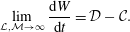 $$\begin{eqnarray}\lim _{{\mathcal{L}},{\mathcal{M}}\rightarrow \infty }\frac{\text{d}W}{\text{d}t}={\mathcal{D}}-{\mathcal{C}}.\end{eqnarray}$$
The question of free energy conservation is more complicated when using sophisticated closures in the style of Hammett & Perkins (Reference Hammett and Perkins1990), as in Beer’s gyrofluid model. The calculation of free energy conservation in our Laguerre–Hermite model in this section demonstrates that the Beer gyrofluid model conserves free energy in the absence of driving and collisions when all closure terms are dropped (after making some reinterpretations addressed in appendix G). However, one would like to be able to show that the free energy does not increase when Beer’s closure terms are included. This is complicated by the fact that the Beer closure scheme includes both dissipative and non-dissipative (reactive) terms. While the dissipative terms by nature can only decrease the free energy, the non-dissipative terms are more troubling. Nonetheless, the dissipative and non-dissipative terms collectively serve to mimic physical damping from phase mixing, so one would expect that the aggregate contribution of these terms is to decrease the free energy. It is then enough to show that the eigenvalues of the closed system are all damped in the absence of driving and collisions.
4.1 Summary of free energy issues
We have shown that the Laguerre–Hermite projection produces a set of coupled equations of moments, each of which has three spatial dimensions and evolves in time. If one truncates the collisionless system of equations [by simply neglecting all terms in the Laguerre–Hermite series with $\ell \geqslant {\mathcal{L}}$
or
$\ell \geqslant {\mathcal{L}}$
or $m\geqslant {\mathcal{M}}$
(provided
$m\geqslant {\mathcal{M}}$
(provided ${\mathcal{L}}>1$
and
${\mathcal{L}}>1$
and ${\mathcal{M}}>2$
)], and considers the case for which there are no driving gradients, these equations conserve the truncated gyrokinetic free energy given in (4.3). The orthogonality of the Laguerre and Hermite basis functions gives the structure that is missing from the Beer gyrofluid equations, which did not conserve a free energy functional (see appendix G).
${\mathcal{M}}>2$
)], and considers the case for which there are no driving gradients, these equations conserve the truncated gyrokinetic free energy given in (4.3). The orthogonality of the Laguerre and Hermite basis functions gives the structure that is missing from the Beer gyrofluid equations, which did not conserve a free energy functional (see appendix G).
In this truncated system, if one then includes collisions, the truncated gyrokinetic free energy is explicitly damped, even as the truncated expressions for number [(3.23), except with the $\ell$
sum running from
$\ell$
sum running from $0$
to
$0$
to ${\mathcal{L}}-1$
], parallel and perpendicular momenta [(3.39) and (3.40), with the same
${\mathcal{L}}-1$
], parallel and perpendicular momenta [(3.39) and (3.40), with the same $\ell$
truncation] and energy [(3.34), using the projections in (3.42) and (3.41), with the same
$\ell$
truncation] and energy [(3.34), using the projections in (3.42) and (3.41), with the same $\ell$
truncation] are conserved.
$\ell$
truncation] are conserved.
With non-zero, fixed-in-time gradients, the free energy density $W(t)$
is no longer formally bounded, even with finite collisions. This might happen, for example, if one had strong gradients, weak collisions, and only a few Laguerre–Hermite moments. In the the context of the gyrokinetic free energy, we have described the desired properties of Landau fluid closures that might be used to model the transfer of free energy density to unresolved scales in velocity space (
$W(t)$
is no longer formally bounded, even with finite collisions. This might happen, for example, if one had strong gradients, weak collisions, and only a few Laguerre–Hermite moments. In the the context of the gyrokinetic free energy, we have described the desired properties of Landau fluid closures that might be used to model the transfer of free energy density to unresolved scales in velocity space ( $\ell \geqslant {\mathcal{L}}$
or
$\ell \geqslant {\mathcal{L}}$
or $m\geqslant {\mathcal{M}}$
). In such cases, collisions, which are more important at small scales in velocity space, would ultimately provide a physical sink.
$m\geqslant {\mathcal{M}}$
). In such cases, collisions, which are more important at small scales in velocity space, would ultimately provide a physical sink.
5 Linear results
We now show some preliminary linear calculations, as a proof of concept of our Laguerre–Hermite formulation of gyrokinetics. These calculations have been performed with GX, a new gyrokinetic code that uses our Laguerre–Hermite spectral velocity discretization. Numerical details and further results from GX will be reported separately. All of the results from this section use closure by truncation.
5.1 Local linear ITG
We first examine an ion temperature gradient (ITG) instability in the local limit, where $k_{\Vert }$
,
$k_{\Vert }$
, $B$
and
$B$
and $\unicode[STIX]{x1D714}_{d}$
are treated as constants. We select a case used to validate the Beer
$\unicode[STIX]{x1D714}_{d}$
are treated as constants. We select a case used to validate the Beer $4+2$
gyrofluid model (Beer & Hammett Reference Beer and Hammett1996), which first appeared in Dong, Horton & Kim (Reference Dong, Horton and Kim1992). The relevant parameters (in our units) are
$4+2$
gyrofluid model (Beer & Hammett Reference Beer and Hammett1996), which first appeared in Dong, Horton & Kim (Reference Dong, Horton and Kim1992). The relevant parameters (in our units) are $q=2$
,
$q=2$
, $R_{0}/a=5$
,
$R_{0}/a=5$
, $k_{\Vert }a=a/qR_{0}$
,
$k_{\Vert }a=a/qR_{0}$
, $a/L_{n}=1$
and
$a/L_{n}=1$
and $a/L_{T}=1.5,2$
, and 3. We also set
$a/L_{T}=1.5,2$
, and 3. We also set $\unicode[STIX]{x1D708}=0.01$
. Figure 1 shows linear growth rates over a range of
$\unicode[STIX]{x1D708}=0.01$
. Figure 1 shows linear growth rates over a range of $k_{y}\unicode[STIX]{x1D70C}_{i}$
for two choices of Laguerre–Hermite velocity resolution. For comparison, we also show the results from the Beer gyrofluid model. We see that the growth rates converge as the Laguerre–Hermite resolution is increased.
$k_{y}\unicode[STIX]{x1D70C}_{i}$
for two choices of Laguerre–Hermite velocity resolution. For comparison, we also show the results from the Beer gyrofluid model. We see that the growth rates converge as the Laguerre–Hermite resolution is increased.
We calculate a normalized integrated velocity-space spectrum,
 $$\begin{eqnarray}P(\ell ,m)=\frac{\displaystyle \int \text{d}^{3}\boldsymbol{R}\,|G_{\ell ,m}|^{2}}{\displaystyle \int \text{d}^{3}\boldsymbol{R}\,|G_{0,0}|^{2}},\end{eqnarray}$$
to examine the structure of the distribution function in the Laguerre–Hermite basis. $P$
can also be interpreted as a measure of the free energy in each moment. Figure 2 shows this spectrum for the higher resolution case in the above
$P$
can also be interpreted as a measure of the free energy in each moment. Figure 2 shows this spectrum for the higher resolution case in the above $a/L_{T}=2$
calculation. The amplitude
$a/L_{T}=2$
calculation. The amplitude $P$
is highest at small
$P$
is highest at small $\ell$
and
$\ell$
and $m$
, which is expected since free energy is injected by the gradients at these large scales. The upper right quadrant of the plot, where both
$m$
, which is expected since free energy is injected by the gradients at these large scales. The upper right quadrant of the plot, where both $\ell$
and
$\ell$
and $m$
are large, is more than six orders of magnitude smaller than the large amplitudes at small
$m$
are large, is more than six orders of magnitude smaller than the large amplitudes at small $\ell$
and
$\ell$
and $m$
. For best contrast we have truncated the colour scale to seven orders of magnitude, but note that the amplitude in the top right corner, corresponding to the finest resolved scale in the velocity space, is
$m$
. For best contrast we have truncated the colour scale to seven orders of magnitude, but note that the amplitude in the top right corner, corresponding to the finest resolved scale in the velocity space, is $P(15,31)\sim 10^{-10}$
. This is a good indication that this calculation is well resolved in velocity space. Further, we see that
$P(15,31)\sim 10^{-10}$
. This is a good indication that this calculation is well resolved in velocity space. Further, we see that $P(7,15)\sim 10^{-5}$
. This is the finest resolved scale in the lower resolution case, which has a spectrum (not shown) that looks qualitatively similar to the lower left quadrant of figure 2, and which also has
$P(7,15)\sim 10^{-5}$
. This is the finest resolved scale in the lower resolution case, which has a spectrum (not shown) that looks qualitatively similar to the lower left quadrant of figure 2, and which also has $P(7,15)\sim 10^{-5}$
. The fact that the lower resolution case agrees with the higher resolution case in both growth rates and spectra suggests that the low resolution case has sufficient resolution.
$P(7,15)\sim 10^{-5}$
. The fact that the lower resolution case agrees with the higher resolution case in both growth rates and spectra suggests that the low resolution case has sufficient resolution.
5.2 Cyclone linear ITG
We also examine an ITG instability in the non-local limit, for which we use the Cyclone base case parameters, a widely benchmarked test case (Dimits et al.
Reference Dimits, Bateman, Beer, Cohen, Dorland, Hammett, Kim, Kinsey, Kotschenreuther and Kritz2000). Figure 3 shows the linear growth rates over a range of $k_{y}\unicode[STIX]{x1D70C}_{i}$
for the same two choices of Laguerre–Hermite velocity resolution as above. For comparison, we also show the results from the Beer
$k_{y}\unicode[STIX]{x1D70C}_{i}$
for the same two choices of Laguerre–Hermite velocity resolution as above. For comparison, we also show the results from the Beer $4+2$
gyrofluid model, along with results from the gyrokinetic code GS2. GS2 solves the gyrokinetic equation using a polar velocity grid in energy and pitch angle coordinates,
$4+2$
gyrofluid model, along with results from the gyrokinetic code GS2. GS2 solves the gyrokinetic equation using a polar velocity grid in energy and pitch angle coordinates, $\unicode[STIX]{x1D700}$
and
$\unicode[STIX]{x1D700}$
and $\unicode[STIX]{x1D706}=\unicode[STIX]{x1D707}/\unicode[STIX]{x1D700}$
. In the limit of large velocity resolution, our Laguerre–Hermite approach should agree with the grid-based approach of GS2. From the figure we see that the two approaches do indeed agree in the higher resolution case. We also see that the convergence in resolution is slower here in the non-local limit than in the local limit above, as the lower resolution case gives growth rates too large for higher
$\unicode[STIX]{x1D706}=\unicode[STIX]{x1D707}/\unicode[STIX]{x1D700}$
. In the limit of large velocity resolution, our Laguerre–Hermite approach should agree with the grid-based approach of GS2. From the figure we see that the two approaches do indeed agree in the higher resolution case. We also see that the convergence in resolution is slower here in the non-local limit than in the local limit above, as the lower resolution case gives growth rates too large for higher $k_{y}\unicode[STIX]{x1D70C}_{i}$
. This suggests that more velocity resolution is needed in the non-local limit than in the local limit.
$k_{y}\unicode[STIX]{x1D70C}_{i}$
. This suggests that more velocity resolution is needed in the non-local limit than in the local limit.

Figure 1. Growth rates of an ITG instability in the local limit. The results from the Laguerre–Hermite formulation are shown at two choices of velocity resolution (blue and green), as well results from the Beer $4+2$
gyrofluid model (red). The Laguerre–Hermite results show good convergence in velocity resolution, especially at small
$4+2$
gyrofluid model (red). The Laguerre–Hermite results show good convergence in velocity resolution, especially at small $k_{y}\unicode[STIX]{x1D70C}_{i}$
.
$k_{y}\unicode[STIX]{x1D70C}_{i}$
.
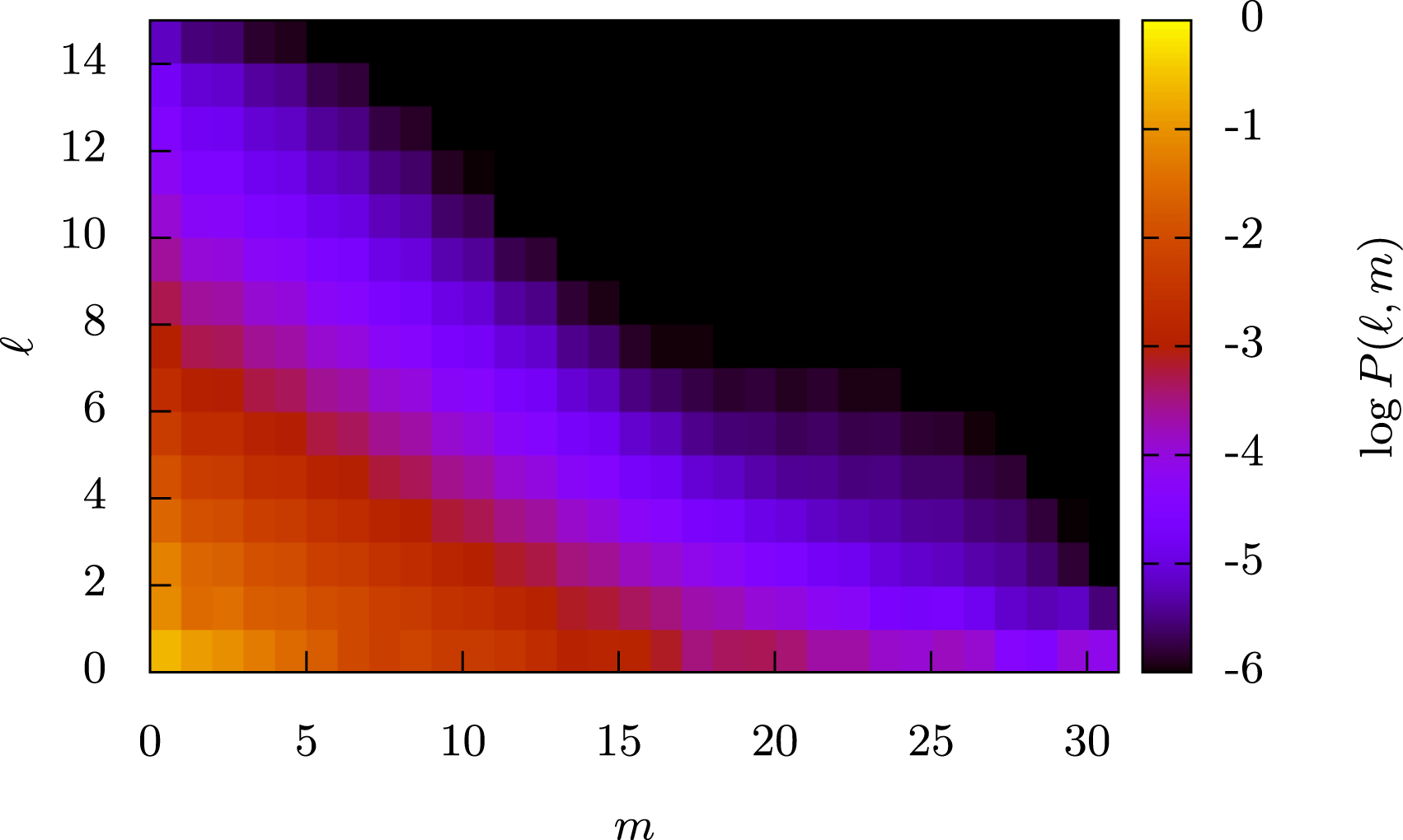
Figure 2. The normalized integrated velocity-space spectrum, defined by (5.1), resulting from the higher resolution $a/L_{T}=2$
case in figure 1. The amplitudes decrease by several orders of magnitude moving from small to large
$a/L_{T}=2$
case in figure 1. The amplitudes decrease by several orders of magnitude moving from small to large $\ell$
and
$\ell$
and $m$
, indicating that the calculation is well resolved in velocity space.
$m$
, indicating that the calculation is well resolved in velocity space.
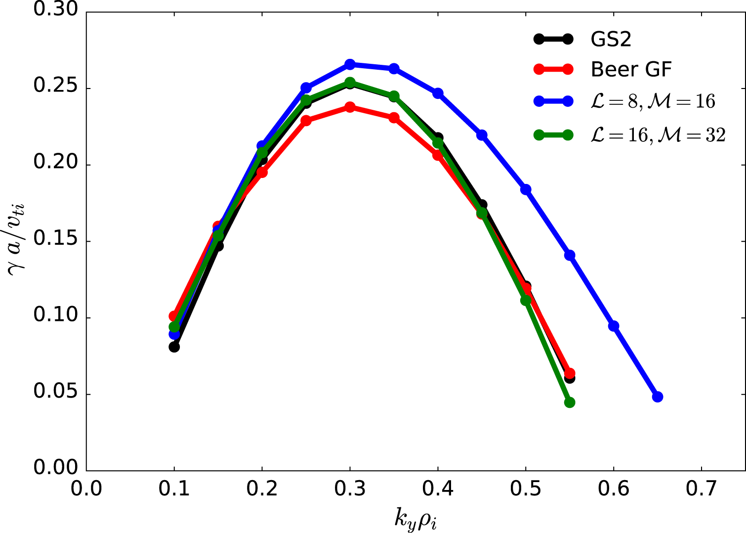
Figure 3. Linear growth rates for the Cyclone base case (Dimits et al.
Reference Dimits, Bateman, Beer, Cohen, Dorland, Hammett, Kim, Kinsey, Kotschenreuther and Kritz2000). The results from the Laguerre–Hermite formulation are shown at two choices of velocity resolution (blue and green), as well as results from the gyrokinetic code GS2 (black) and the Beer $4+2$
gyrofluid model (red).
$4+2$
gyrofluid model (red).

This is confirmed by the velocity spectrum for this case, shown in figure 4. Whereas in the local limit a significant portion of the velocity space had amplitudes more than six orders of magnitude smaller than the largest amplitudes, in the non-local limit the amplitudes decrease much more gradually. This indicates that the distribution function has more structure in velocity space in this case. This also shows why the lower resolution case failed to produce accurate growth rates: the amplitudes in the lower left quadrant of figure 4 do not decrease by as much as in the local case, with $P(7,15)\sim 10^{-4}$
.
$P(7,15)\sim 10^{-4}$
.
5.3 Rosenbluth–Hinton zonal flow residual
As a final test, we examine zonal flow dynamics in our Laguerre–Hermite formulation. Zonal flows are nonlinearly driven and nonlinearly damped (Rogers, Dorland & Kotschenreuther Reference Rogers, Dorland and Kotschenreuther2000) toroidally and poloidally symmetric sheared $\boldsymbol{E}\times \boldsymbol{B}$
flows that have been shown to play a key role in determining the turbulence saturation level (Hammett et al.
Reference Hammett, Beer, Dorland, Cowley and Smith1993; Waltz, Kerbel & Milovich Reference Waltz, Kerbel and Milovich1994). Rosenbluth & Hinton (Reference Rosenbluth and Hinton1998) first showed that zonal flows are not linearly damped by collisionless processes, showing that in a simplified equilibrium model the residual flow is given by
$\boldsymbol{E}\times \boldsymbol{B}$
flows that have been shown to play a key role in determining the turbulence saturation level (Hammett et al.
Reference Hammett, Beer, Dorland, Cowley and Smith1993; Waltz, Kerbel & Milovich Reference Waltz, Kerbel and Milovich1994). Rosenbluth & Hinton (Reference Rosenbluth and Hinton1998) first showed that zonal flows are not linearly damped by collisionless processes, showing that in a simplified equilibrium model the residual flow is given by
 $$\begin{eqnarray}\frac{\unicode[STIX]{x1D6F7}(t=\infty )}{\unicode[STIX]{x1D6F7}(t=0)}=\frac{1}{1+1.6q^{2}/\sqrt{\unicode[STIX]{x1D716}}},\end{eqnarray}$$
where $q$
is the safety factor and
$q$
is the safety factor and $\unicode[STIX]{x1D716}=r/R_{0}$
is the inverse aspect ratio. The original Beer gyrofluid model did not accurately capture the residual because of the damping introduced by the closures. This caused discrepancies with gyrokinetic models in nonlinear simulations (Dimits et al.
Reference Dimits, Bateman, Beer, Cohen, Dorland, Hammett, Kim, Kinsey, Kotschenreuther and Kritz2000). The gyrofluid closure was modified to be able to capture some of the zonal flow residual with limited success (Beer & Hammett Reference Beer, Hammett, Connor, Sindoni and Vaclavik1998).
$\unicode[STIX]{x1D716}=r/R_{0}$
is the inverse aspect ratio. The original Beer gyrofluid model did not accurately capture the residual because of the damping introduced by the closures. This caused discrepancies with gyrokinetic models in nonlinear simulations (Dimits et al.
Reference Dimits, Bateman, Beer, Cohen, Dorland, Hammett, Kim, Kinsey, Kotschenreuther and Kritz2000). The gyrofluid closure was modified to be able to capture some of the zonal flow residual with limited success (Beer & Hammett Reference Beer, Hammett, Connor, Sindoni and Vaclavik1998).

Figure 5. Rosenbluth–Hinton residual flow for various values of $\unicode[STIX]{x1D716}=r/R_{0}$
. The residuals calculated by the Laguerre–Hermite model with
$\unicode[STIX]{x1D716}=r/R_{0}$
. The residuals calculated by the Laguerre–Hermite model with ${\mathcal{L}}=16$
and
${\mathcal{L}}=16$
and ${\mathcal{M}}=32$
agree well with those calculated by GS2. We also show the expected theoretical result, equation (5.2).
${\mathcal{M}}=32$
agree well with those calculated by GS2. We also show the expected theoretical result, equation (5.2).
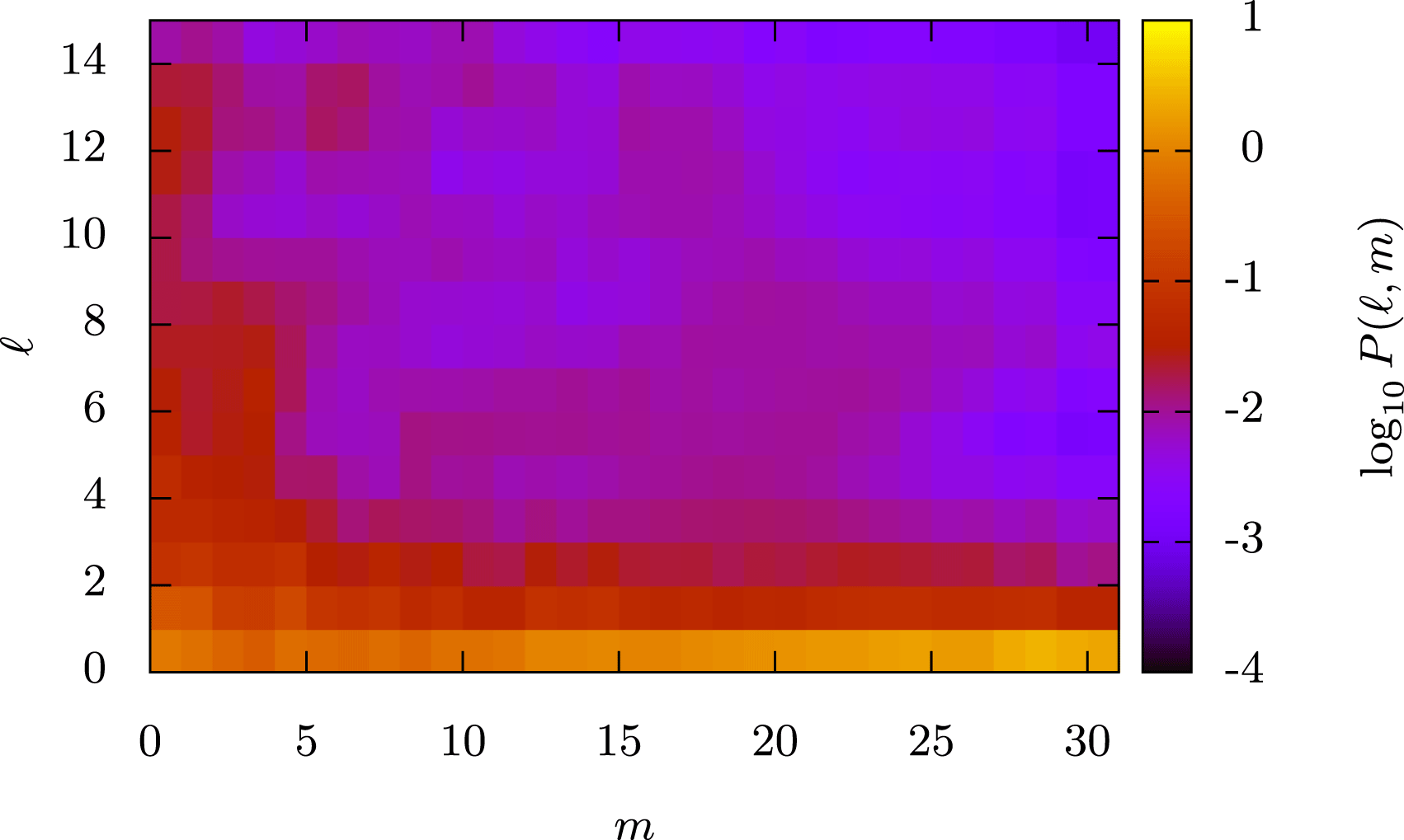
Figure 6. The normalized integrated velocity-space spectrum for the $\unicode[STIX]{x1D716}=0.2$
case from figure 5. High amplitudes at large
$\unicode[STIX]{x1D716}=0.2$
case from figure 5. High amplitudes at large $m$
along the axis are the result of trapped particle dynamics that produces sharp features in
$m$
along the axis are the result of trapped particle dynamics that produces sharp features in $v_{\Vert }$
.
$v_{\Vert }$
.
Figure 5 shows residuals for several values of $\unicode[STIX]{x1D716}$
, for the
$\unicode[STIX]{x1D716}$
, for the $k_{x}\unicode[STIX]{x1D70C}_{i}=0.01$
mode with
$k_{x}\unicode[STIX]{x1D70C}_{i}=0.01$
mode with $q=1.4$
, as calculated by our Laguerre–Hermite model with
$q=1.4$
, as calculated by our Laguerre–Hermite model with ${\mathcal{L}}=16$
and
${\mathcal{L}}=16$
and ${\mathcal{M}}=32$
. We also show the residual calculated by GS2 and the expected theoretical value from (5.2). Our result for the average residual agrees well with GS2, though we note that we observe larger oscillations and less damping of the potential in the Laguerre–Hermite model. We attribute this to resolution issues. The velocity spectrum, shown in figure 6 for the
${\mathcal{M}}=32$
. We also show the residual calculated by GS2 and the expected theoretical value from (5.2). Our result for the average residual agrees well with GS2, though we note that we observe larger oscillations and less damping of the potential in the Laguerre–Hermite model. We attribute this to resolution issues. The velocity spectrum, shown in figure 6 for the $\unicode[STIX]{x1D716}=0.2$
case, shows overall larger amplitudes compared to the spectra from the linear instability calculations. We also see that there are high amplitudes at large
$\unicode[STIX]{x1D716}=0.2$
case, shows overall larger amplitudes compared to the spectra from the linear instability calculations. We also see that there are high amplitudes at large $m$
along the axis, indicating that sharp features are being generated in
$m$
along the axis, indicating that sharp features are being generated in $g(v_{\Vert })$
. This is to be expected, since the zonal flow residual is the result of complicated kinetic effects involving trapped particle dynamics, and resolving the trapped–passing boundary (which the velocity grid in GS2 is explicitly designed for) is important. Naturally, our spectral approach is not as well suited to resolving these sharp features. In the problems we will target, however, collisions and nonlinearity will help to smear away sharp features in the distribution function.
$g(v_{\Vert })$
. This is to be expected, since the zonal flow residual is the result of complicated kinetic effects involving trapped particle dynamics, and resolving the trapped–passing boundary (which the velocity grid in GS2 is explicitly designed for) is important. Naturally, our spectral approach is not as well suited to resolving these sharp features. In the problems we will target, however, collisions and nonlinearity will help to smear away sharp features in the distribution function.
5.4 Summary of results
These preliminary results show that our model is capable of reproducing gyrokinetic results for linear instabilities and zonal flow dynamics at spectral resolution comparable to conventional gyrokinetic velocity resolution, even with the simplest possible closure scheme. In the linear instability comparisons we see that the Beer $4+2$
gyrofluid model is nearly as accurate at much lower resolution. Since our spectral system is effectively a generalized gyrofluid model, implementing gyrofluid-like closures in our system will be straightforward. Thus the Beer results are encouraging, since they indicate that using more advanced closure schemes in our system can lead to gyrokinetic accuracy at sub-kinetic velocity resolution. However, there are cases where we will still need to use higher velocity resolution, such as in the zonal flow results. In this case, the failure of the Beer model to produce the undamped residual shows the shortcomings of using low velocity resolution with gyrofluid-like closures when the correct solution has sharp features in velocity space.
$4+2$
gyrofluid model is nearly as accurate at much lower resolution. Since our spectral system is effectively a generalized gyrofluid model, implementing gyrofluid-like closures in our system will be straightforward. Thus the Beer results are encouraging, since they indicate that using more advanced closure schemes in our system can lead to gyrokinetic accuracy at sub-kinetic velocity resolution. However, there are cases where we will still need to use higher velocity resolution, such as in the zonal flow results. In this case, the failure of the Beer model to produce the undamped residual shows the shortcomings of using low velocity resolution with gyrofluid-like closures when the correct solution has sharp features in velocity space.
6 Summary and conclusion
In this report, we have outlined a new pseudo-spectral velocity formulation of flux-tube gyrokinetics. This is achieved by projecting the gyrokinetic equation onto a velocity basis composed of Laguerre and Hermite polynomials. A key advantage of the resulting model is the flexibility in choice of velocity-space resolution. At the lowest velocity-space resolution, the model corresponds directly to gyrofluid models. Within the same framework, the model corresponds to conventional gyrokinetic approaches at high velocity resolution. Between these limits, one has the freedom to tailor the resolution to one’s needs: one can smoothly increase resolution to improve accuracy, or one can minimize resolution to produce a performance advantage. There is also an opportunity for a dynamic fidelity refinement approach, where the resolution can be adjusted dynamically during a simulation.
The flexibility to use relatively lower velocity resolution than is used in standard gyrokinetic approaches is due to the fact that our Laguerre–Hermite formulation expresses critical conservation laws (density, momentum, energy and free energy) even at very low resolution. We have presented a model collision operator that reflects this prioritization: it expresses the key conservation laws at long wavelength, but sharply attenuates higher moments at short wavelengths as a result of classical diffusion, pitch-angle scattering, energy diffusion, and slowing down. Our collision operator is also efficiently expressed in our basis, and it satisfies the H theorem.
The main disadvantage of our approach is the need for closures due to the coupling of the spectral moments, which arises as the mathematical manifestation of the physics of phase mixing. We recognize that the value of our approach will only be fully realized when a generalized closure scheme has been found that can give gyrokinetic fidelity with sub-kinetic velocity resolution. The relative success of gyrofluid closures indicates that this is feasible, and we can use these closures directly in our model at the lowest resolution (see appendix F). We thus leave as important future work the generalization of gyrofluid-like closures to arbitrary spectral velocity resolution. This will bolster the flexibility of the model, as one will be able to capture important kinetic effects with whatever fidelity is required by the problem at hand. This includes modelling linear phase mixing from Landau damping and toroidal drifts as well as nonlinear effects such as nonlinear FLR phase mixing (Dorland & Hammett Reference Dorland and Hammett1993; Schekochihin et al. Reference Schekochihin, Cowley, Dorland, Hammett, Howes, Quataert and Tatsuno2009; Tatsuno et al. Reference Tatsuno, Dorland, Schekochihin, Plunk, Barnes, Cowley and Howes2009; Chen et al. Reference Chen, Wicks, Horbury and Schekochihin2010; Plunk et al. Reference Plunk, Cowley, Schekochihin and Tatsuno2010; Howes et al. Reference Howes, TenBarge, Dorland, Quataert, Schekochihin, Numata and Tatsuno2011; Kawamori Reference Kawamori2013; Numata & Loureiro Reference Numata and Loureiro2015), and phase un-mixing from the plasma echo (Kanekar Reference Kanekar2014; Parker & Dellar Reference Parker and Dellar2015; Schekochihin et al. Reference Schekochihin, Parker, Highcock, Dellar, Dorland and Hammett2016).
We also leave the extension of this model to include electromagnetic fluctuations for the future. While we could simply include electrons as a second species and find the perpendicular magnetic field fluctuations from Ampere’s law, such an approach is potentially expensive. For many applications, the Snyder & Hammett (Reference Snyder and Hammett2001) model will be the best way forward, for example. Importantly, a model with $\unicode[STIX]{x1D6FF}A_{\Vert }$
and
$\unicode[STIX]{x1D6FF}A_{\Vert }$
and $\unicode[STIX]{x1D6FF}B_{\Vert }$
presents no new challenges to the Laguerre–Hermite projections.
$\unicode[STIX]{x1D6FF}B_{\Vert }$
presents no new challenges to the Laguerre–Hermite projections.
Our preliminary results show that our model is capable of reproducing gyrokinetic results for linear instabilities and zonal flow dynamics at spectral resolution comparable to conventional gyrokinetic velocity grid resolution, even with the simplest possible closure scheme. More advanced closure schemes could lead to similar accuracy at lower cost in cases where there are not sharp features in velocity space. Nonlinear simulations of ion temperature gradient turbulence, which make use of the pseudo-spectral approach described in appendix D, will be reported in a later work. In the nonlinear system, turbulence is an additional source of regularization in velocity space, which should allow the use of lower velocity resolution in the pseudo-spectral system than in a standard grid-based approach. We have also coupled our model to the TRINITY full-torus gyrokinetic transport framework (Barnes et al. Reference Barnes, Abel, Dorland, Görler, Hammett and Jenko2010). In this setting the flexibility of our model enables a significant performance advantage over standard approaches, allowing efficient and tractable whole-device modelling of tokamaks and stellarators (Highcock et al. Reference Highcock, Mandell, Barnes and Dorland2016).
Finally, we note that our model is inherently parallelizable and has a small memory footprint due to its pseudo-spectral approach. This allows us to move a well-resolved gyrokinetic simulation of ion temperature gradient-driven tokamak turbulence from hundreds or thousands of cores on an massively parallel HPC device to a single graphics processor (GPU). Thus our new Laguerre–Hermite pseudo-spectral formulation has produced a high-fidelity gyrokinetic simulation code that runs at a few teraflops on a desktop computer with an inexpensive GPU.
Acknowledgements
We would like to thank I. Abel, P. Helander, E. Highcock, G. Hammett, A. Schekochihin, M. Barnes and K. Despain for fruitful discussions and encouragement. Research support came from the US Department of Energy: N.R.M. is supported by the DOE CSGF program, provided under grant DE-FG02-97ER25308; W.D. is supported by award numbers DE-FC02-08ER54964 and DE-FG02-93ER54197; M.L. is supported by award number DE-FG02-93ER54197. Computations were performed at the Texas Advanced Computing Center (TACC) at The University of Texas at Austin, via the Extreme Science and Engineering Discovery Environment (XSEDE), which is supported by National Science Foundation grant number ACI-1548562.
Appendix A. Non-dimensionalization
In $(v_{\Vert },\unicode[STIX]{x1D707})$
coordinates, the gyrokinetic equation can be written (Brizard Reference Brizard1992; Beer & Hammett Reference Beer and Hammett1996; Snyder & Hammett Reference Snyder and Hammett2001; Parra & Barnes Reference Parra and Barnes2015) as:
$(v_{\Vert },\unicode[STIX]{x1D707})$
coordinates, the gyrokinetic equation can be written (Brizard Reference Brizard1992; Beer & Hammett Reference Beer and Hammett1996; Snyder & Hammett Reference Snyder and Hammett2001; Parra & Barnes Reference Parra and Barnes2015) as:
 $$\begin{eqnarray}\frac{\unicode[STIX]{x2202}g}{\unicode[STIX]{x2202}t}+[v_{\Vert }\hat{\boldsymbol{b}}+\langle \boldsymbol{v}_{E}\rangle _{\boldsymbol{R}}+\boldsymbol{v}_{d}]\boldsymbol{\cdot }\unicode[STIX]{x1D735}h+\langle \boldsymbol{v}_{E}\rangle _{\boldsymbol{R}}\boldsymbol{\cdot }\unicode[STIX]{x1D735}F_{M}-\unicode[STIX]{x1D707}(\hat{\boldsymbol{b}}\boldsymbol{\cdot }\unicode[STIX]{x1D735}B)\frac{\unicode[STIX]{x2202}h}{\unicode[STIX]{x2202}v_{\Vert }}=C(h).\end{eqnarray}$$
In this equation, the distribution function $F=F_{0}+\unicode[STIX]{x1D6FF}f=F_{M}(1-q\unicode[STIX]{x1D6F7}/T)+h$
, and the perturbed, gyroaveraged distribution function
$F=F_{0}+\unicode[STIX]{x1D6FF}f=F_{M}(1-q\unicode[STIX]{x1D6F7}/T)+h$
, and the perturbed, gyroaveraged distribution function $g=\langle \unicode[STIX]{x1D6FF}f\rangle _{\boldsymbol{R}}=h-q\langle \unicode[STIX]{x1D6F7}\rangle _{\boldsymbol{R}}F_{M}/T$
, where
$g=\langle \unicode[STIX]{x1D6FF}f\rangle _{\boldsymbol{R}}=h-q\langle \unicode[STIX]{x1D6F7}\rangle _{\boldsymbol{R}}F_{M}/T$
, where $\langle \cdots \rangle _{\boldsymbol{R}}$
denotes a gyroaverage at fixed guiding centre position
$\langle \cdots \rangle _{\boldsymbol{R}}$
denotes a gyroaverage at fixed guiding centre position $\boldsymbol{R}$
, and
$\boldsymbol{R}$
, and $F_{M}$
is a Maxwellian distribution function.
$F_{M}$
is a Maxwellian distribution function.
Radial gradients of the equilibrium distribution function are assumed to vary on a scale $a$
(which may be taken to be the minor radius, major radius, or some other convenient macroscale length). All equilibrium-scale lengths, such as density gradient scale lengths, magnetic curvature and so on, are normalized by
$a$
(which may be taken to be the minor radius, major radius, or some other convenient macroscale length). All equilibrium-scale lengths, such as density gradient scale lengths, magnetic curvature and so on, are normalized by $a$
. The magnetic field
$a$
. The magnetic field $B$
is normalized by
$B$
is normalized by $B_{a}$
, which may be chosen for convenience. A typical choice would be the vacuum magnetic field at the centre of the last closed flux surface, at the elevation of the magnetic axis.
$B_{a}$
, which may be chosen for convenience. A typical choice would be the vacuum magnetic field at the centre of the last closed flux surface, at the elevation of the magnetic axis.
Fluctuating quantities are assumed to vary along the field line slowly and across the field line rapidly. We thus normalize variations of fluctuations along the field line by $a$
, and across field lines by
$a$
, and across field lines by $\unicode[STIX]{x1D70C}_{\text{ref}}$
, where
$\unicode[STIX]{x1D70C}_{\text{ref}}$
, where $\unicode[STIX]{x1D70C}_{\text{ref}}$
is the thermal gyroradius of a convenient reference species, which is in turn characterized by its charge
$\unicode[STIX]{x1D70C}_{\text{ref}}$
is the thermal gyroradius of a convenient reference species, which is in turn characterized by its charge $q_{\text{ref}}$
, mass
$q_{\text{ref}}$
, mass $M_{\text{ref}}$
, temperature
$M_{\text{ref}}$
, temperature $T_{0,\text{ref}}$
, density
$T_{0,\text{ref}}$
, density $n_{0,\text{ref}}$
. Throughout this paper, we define thermal speeds by
$n_{0,\text{ref}}$
. Throughout this paper, we define thermal speeds by $v_{t}\equiv \sqrt{T/M}$
, so that
$v_{t}\equiv \sqrt{T/M}$
, so that
 $$\begin{eqnarray}\unicode[STIX]{x1D70C}_{\text{ref}}=v_{t,\text{ref}}/\unicode[STIX]{x1D6FA}_{\text{ref}}=\left(\sqrt{\frac{T_{0,\text{ref}}}{M_{\text{ref}}}}\right)\frac{M_{\text{ref}}c}{q_{\text{ref}}B_{a}}.\end{eqnarray}$$
In this expression, $c$
represents the speed of light.
$c$
represents the speed of light.
The gyrokinetic expansion parameter $\unicode[STIX]{x1D700}$
can be taken to be
$\unicode[STIX]{x1D700}$
can be taken to be $\unicode[STIX]{x1D700}=\unicode[STIX]{x1D70C}_{\text{ref}}/a\equiv \unicode[STIX]{x1D70C}_{\ast }$
. Fluctuations vary slowly in time compared to the gyrofrequency. Accordingly, the fluctuation time scale is normalized by
$\unicode[STIX]{x1D700}=\unicode[STIX]{x1D70C}_{\text{ref}}/a\equiv \unicode[STIX]{x1D70C}_{\ast }$
. Fluctuations vary slowly in time compared to the gyrofrequency. Accordingly, the fluctuation time scale is normalized by $\unicode[STIX]{x1D6FA}_{\text{ref}}\unicode[STIX]{x1D70C}_{\ast }=v_{t,\text{ref}}/a$
. Similarly, fluctuating quantities are small compared to equilibrium quantities (e.g. fluctuating density
$\unicode[STIX]{x1D6FA}_{\text{ref}}\unicode[STIX]{x1D70C}_{\ast }=v_{t,\text{ref}}/a$
. Similarly, fluctuating quantities are small compared to equilibrium quantities (e.g. fluctuating density $\unicode[STIX]{x1D6FF}n\sim \unicode[STIX]{x1D700}n_{0}$
). The equations are therefore most naturally expressed by scaling the fluctuating quantities by
$\unicode[STIX]{x1D6FF}n\sim \unicode[STIX]{x1D700}n_{0}$
). The equations are therefore most naturally expressed by scaling the fluctuating quantities by $1/\unicode[STIX]{x1D70C}_{\text{ref}}$
. This includes the electrostatic potential, which is normalized by
$1/\unicode[STIX]{x1D70C}_{\text{ref}}$
. This includes the electrostatic potential, which is normalized by $T_{0,\text{ref}}/q_{\text{ref}}$
. That is, the physical electrostatic potential
$T_{0,\text{ref}}/q_{\text{ref}}$
. That is, the physical electrostatic potential $\unicode[STIX]{x1D6F7}_{\text{phys}}=(T_{0,\text{ref}}/q_{\text{ref}})\tilde{\unicode[STIX]{x1D6F7}}\unicode[STIX]{x1D70C}_{\ast }$
, where
$\unicode[STIX]{x1D6F7}_{\text{phys}}=(T_{0,\text{ref}}/q_{\text{ref}})\tilde{\unicode[STIX]{x1D6F7}}\unicode[STIX]{x1D70C}_{\ast }$
, where $\tilde{\unicode[STIX]{x1D6F7}}$
is the normalized fluctuating electrostatic potential.
$\tilde{\unicode[STIX]{x1D6F7}}$
is the normalized fluctuating electrostatic potential.
For each species, we normalize the velocity-space coordinates $v_{\Vert }$
and
$v_{\Vert }$
and $\unicode[STIX]{x1D707}$
using the thermal velocity for that species. This thermal velocity is in turn normalized to the thermal velocity of the reference species. Thus,
$\unicode[STIX]{x1D707}$
using the thermal velocity for that species. This thermal velocity is in turn normalized to the thermal velocity of the reference species. Thus, $v_{\Vert }\hat{\boldsymbol{b}}\boldsymbol{\cdot }\unicode[STIX]{x1D735}\rightarrow (v_{\Vert }/v_{t,s})(v_{t,s}/v_{t,\text{ref}})a\tilde{\unicode[STIX]{x1D735}}_{\Vert }$
. In the body of this report, we simplify the final equations by cancelling common factors and by dropping the tilde notation. Thus, this operator would appear in explicit form as
$v_{\Vert }\hat{\boldsymbol{b}}\boldsymbol{\cdot }\unicode[STIX]{x1D735}\rightarrow (v_{\Vert }/v_{t,s})(v_{t,s}/v_{t,\text{ref}})a\tilde{\unicode[STIX]{x1D735}}_{\Vert }$
. In the body of this report, we simplify the final equations by cancelling common factors and by dropping the tilde notation. Thus, this operator would appear in explicit form as $v_{ts}v_{\Vert }\hat{\boldsymbol{b}}\boldsymbol{\cdot }\unicode[STIX]{x1D735}$
, where
$v_{ts}v_{\Vert }\hat{\boldsymbol{b}}\boldsymbol{\cdot }\unicode[STIX]{x1D735}$
, where $v_{ts}\equiv v_{t,s}/v_{t,\text{ref}}$
, and it would be understood from context that
$v_{ts}\equiv v_{t,s}/v_{t,\text{ref}}$
, and it would be understood from context that $v_{\Vert }$
had been normalized appropriately for species
$v_{\Vert }$
had been normalized appropriately for species $s$
, and that
$s$
, and that $\hat{\boldsymbol{b}}\boldsymbol{\cdot }\unicode[STIX]{x1D735}$
had been normalized to the length
$\hat{\boldsymbol{b}}\boldsymbol{\cdot }\unicode[STIX]{x1D735}$
had been normalized to the length $a$
. When the context is clear, we may also neglect to write the leading coefficient
$a$
. When the context is clear, we may also neglect to write the leading coefficient $v_{ts}$
.
$v_{ts}$
.
The non-dimensional collision frequency $\unicode[STIX]{x1D708}_{s}$
is given by
$\unicode[STIX]{x1D708}_{s}$
is given by
 $$\begin{eqnarray}\unicode[STIX]{x1D708}_{s}=\frac{n_{s}Z_{s}^{4}v_{ts}}{\unicode[STIX]{x1D70F}_{s}^{2}}\unicode[STIX]{x1D708}_{\text{ref}},\end{eqnarray}$$
where $\unicode[STIX]{x1D708}_{\text{ref}}$
is the collision frequency of the reference species normalized by
$\unicode[STIX]{x1D708}_{\text{ref}}$
is the collision frequency of the reference species normalized by $a/v_{t,\text{ref}}$
:
$a/v_{t,\text{ref}}$
:
 $$\begin{eqnarray}\unicode[STIX]{x1D708}_{\text{ref}}=\frac{\sqrt{2}\unicode[STIX]{x03C0}an_{0,\text{ref}}e^{4}\ln \unicode[STIX]{x1D6EC}}{T_{\text{ref}}^{2}}.\end{eqnarray}$$
The normalized time coordinate is $\tilde{t}=t_{\text{phys}}v_{t,\text{ ref}}/a$
. For species
$\tilde{t}=t_{\text{phys}}v_{t,\text{ ref}}/a$
. For species $s$
, we define the temperature
$s$
, we define the temperature $\unicode[STIX]{x1D70F}_{s}\equiv T_{0,s}/T_{0,\text{ref}}$
, the density
$\unicode[STIX]{x1D70F}_{s}\equiv T_{0,s}/T_{0,\text{ref}}$
, the density $n_{s}\equiv n_{0,s}/n_{0,\text{ref}}$
, the charge
$n_{s}\equiv n_{0,s}/n_{0,\text{ref}}$
, the charge $Z_{s}=q_{s}/q_{\text{ref}}$
, the normalized mass
$Z_{s}=q_{s}/q_{\text{ref}}$
, the normalized mass $m_{s}=M_{s}/M_{\text{ref}}$
and the normalized thermal gyroradius
$m_{s}=M_{s}/M_{\text{ref}}$
and the normalized thermal gyroradius $\unicode[STIX]{x1D70C}_{s}=(v_{t,s}/\unicode[STIX]{x1D6FA}_{s})/\unicode[STIX]{x1D70C}_{\ast }$
.
$\unicode[STIX]{x1D70C}_{s}=(v_{t,s}/\unicode[STIX]{x1D6FA}_{s})/\unicode[STIX]{x1D70C}_{\ast }$
.
Fluctuating densities and temperatures are normalized by their equilibrium values; fluctuations of odd $v_{\Vert }$
moments are normalized by additional appropriate powers of
$v_{\Vert }$
moments are normalized by additional appropriate powers of $v_{ts}$
. The normalized gyrokinetic equation (2.1) results. Elsewhere, we restore normalizations and species subscripts only when needed for clarity.
$v_{ts}$
. The normalized gyrokinetic equation (2.1) results. Elsewhere, we restore normalizations and species subscripts only when needed for clarity.
Appendix B. Linear FLR accuracy
Here we examine the FLR approaches of Brizard and Dorland in the context of the linear dispersion relation in the slab limit with a single hydrogenic ion species and adiabatic electrons. In this limit, the exact kinetic dispersion relation is
 $$\begin{eqnarray}\displaystyle & & \displaystyle 1+\unicode[STIX]{x1D70F}^{-1}+\unicode[STIX]{x1D6E4}_{0}\left\{\left[1-\frac{\unicode[STIX]{x1D714}_{\ast ,n}}{\unicode[STIX]{x1D714}}\left(1-\unicode[STIX]{x1D702}b\left(1-\frac{I_{1}}{\text{I}_{0}}\right)\right)\right]\unicode[STIX]{x1D701}Z(\unicode[STIX]{x1D701})\right.\nonumber\\ \displaystyle & & \displaystyle \qquad \left.-\,\frac{\unicode[STIX]{x1D714}_{\ast ,n}}{\unicode[STIX]{x1D714}}\unicode[STIX]{x1D702}\left[\unicode[STIX]{x1D701}^{2}+\left(\unicode[STIX]{x1D701}^{2}-\frac{1}{2}\right)\right]\unicode[STIX]{x1D701}Z(\unicode[STIX]{x1D701})\right\}=0,\end{eqnarray}$$
where $Z(\unicode[STIX]{x1D701})$
is the plasma dispersion function,
$Z(\unicode[STIX]{x1D701})$
is the plasma dispersion function, $\unicode[STIX]{x1D701}\equiv \unicode[STIX]{x1D714}/(k_{\Vert }\sqrt{2})$
,
$\unicode[STIX]{x1D701}\equiv \unicode[STIX]{x1D714}/(k_{\Vert }\sqrt{2})$
, $\unicode[STIX]{x1D714}_{\ast ,n}\equiv \unicode[STIX]{x1D714}_{\ast }(a/L_{n})$
and
$\unicode[STIX]{x1D714}_{\ast ,n}\equiv \unicode[STIX]{x1D714}_{\ast }(a/L_{n})$
and $\unicode[STIX]{x1D702}\equiv L_{n}/L_{T}$
. Here
$\unicode[STIX]{x1D702}\equiv L_{n}/L_{T}$
. Here $\unicode[STIX]{x1D6E4}_{n}(b)=\text{I}_{n}(b)\text{e}^{-b}$
, where
$\unicode[STIX]{x1D6E4}_{n}(b)=\text{I}_{n}(b)\text{e}^{-b}$
, where $\text{I}_{n}(b)=\text{i}^{-n}\text{J}_{n}(\text{i}b)$
is the modified Bessel function. The ITG marginal stability relation is then given by (Galeev, Oraevskii & Sagdeev Reference Galeev, Oraevskii and Sagdeev1963; Kadomtsev & Pogutse Reference Kadomtsev, Pogutse and Leontovich1970)
$\text{I}_{n}(b)=\text{i}^{-n}\text{J}_{n}(\text{i}b)$
is the modified Bessel function. The ITG marginal stability relation is then given by (Galeev, Oraevskii & Sagdeev Reference Galeev, Oraevskii and Sagdeev1963; Kadomtsev & Pogutse Reference Kadomtsev, Pogutse and Leontovich1970)
 $$\begin{eqnarray}\unicode[STIX]{x1D702}_{\text{crit}}(b)=\frac{\unicode[STIX]{x1D6E4}_{0}}{\displaystyle \frac{\unicode[STIX]{x1D6E4}_{0}}{2}+b(\unicode[STIX]{x1D6E4}_{0}-\unicode[STIX]{x1D6E4}_{1})}.\end{eqnarray}$$
The corresponding dispersion relation for the fluid system with ${\mathcal{L}}$
Laguerre moments and
${\mathcal{L}}$
Laguerre moments and ${\mathcal{M}}$
Hermite moments is
${\mathcal{M}}$
Hermite moments is
 $$\begin{eqnarray}\displaystyle & & \displaystyle 1+\unicode[STIX]{x1D70F}^{-1}+\mathop{\sum }_{\ell =0}^{{\mathcal{L}}-1}{\mathcal{J}}_{\ell }^{2}\left\{\unicode[STIX]{x1D701}Z_{{\mathcal{M}}}(\unicode[STIX]{x1D701})-\frac{\unicode[STIX]{x1D714}_{\ast ,n}}{\unicode[STIX]{x1D714}}\left(\unicode[STIX]{x1D701}Z_{{\mathcal{M}}}(\unicode[STIX]{x1D701})+\unicode[STIX]{x1D702}\left[\unicode[STIX]{x1D701}^{2}+\left(\unicode[STIX]{x1D701}^{2}-\frac{1}{2}\right)\unicode[STIX]{x1D701}Z_{{\mathcal{M}}}(\unicode[STIX]{x1D701})\right]\right)\right\}\nonumber\\ \displaystyle & & \displaystyle \qquad -\,\frac{\unicode[STIX]{x1D714}_{\ast ,n}}{\unicode[STIX]{x1D714}}\unicode[STIX]{x1D702}\mathop{\sum }_{\ell =0}^{{\mathcal{L}}-1}{\mathcal{J}}_{\ell }[\ell {\mathcal{J}}_{\ell -1}+2\ell {\mathcal{J}}_{\ell }+(\ell +1){\mathcal{J}}_{\ell +1}]\unicode[STIX]{x1D701}Z_{{\mathcal{M}}}(\unicode[STIX]{x1D701})=0.\end{eqnarray}$$
Recall from (3.18) that
 $$\begin{eqnarray}{\mathcal{J}}_{\ell }\equiv \frac{b^{\ell }}{\ell !}\frac{\unicode[STIX]{x2202}^{\ell }}{\unicode[STIX]{x2202}b^{\ell }}\langle \text{J}_{0}\rangle ,\end{eqnarray}$$
and $Z_{{\mathcal{M}}}(\unicode[STIX]{x1D701})$
is the fluid approximation to
$Z_{{\mathcal{M}}}(\unicode[STIX]{x1D701})$
is the fluid approximation to $Z(\unicode[STIX]{x1D701})$
with
$Z(\unicode[STIX]{x1D701})$
with ${\mathcal{M}}$
Hermite moments. Note that
${\mathcal{M}}$
Hermite moments. Note that $Z_{{\mathcal{M}}}$
can be written explicitly as a ratio of Hermite polynomials, but we will not need the full expression for this exercise; instead see Smith (Reference Smith1997) for details. The marginal stability relation is then given by
$Z_{{\mathcal{M}}}$
can be written explicitly as a ratio of Hermite polynomials, but we will not need the full expression for this exercise; instead see Smith (Reference Smith1997) for details. The marginal stability relation is then given by
 $$\begin{eqnarray}\unicode[STIX]{x1D702}_{\text{crit}}^{{\mathcal{L}}}(b)=\frac{\displaystyle \mathop{\sum }_{\ell =0}^{{\mathcal{L}}-1}{\mathcal{J}}_{\ell }^{2}}{\displaystyle \frac{1}{2}\mathop{\sum }_{\ell =0}^{{\mathcal{L}}-1}{\mathcal{J}}_{\ell }^{2}-\mathop{\sum }_{\ell =0}^{{\mathcal{L}}-1}{\mathcal{J}}_{\ell }[\ell {\mathcal{J}}_{\ell -1}+2\ell {\mathcal{J}}_{\ell }+(\ell +1){\mathcal{J}}_{\ell +1}]}.\end{eqnarray}$$
Comparing the kinetic result to the fluid one, we see that there are only two FLR expressions to check:
 $$\begin{eqnarray}\displaystyle & \displaystyle \unicode[STIX]{x1D6E4}_{0}\approx \mathop{\sum }_{\ell =0}^{{\mathcal{L}}-1}{\mathcal{J}}_{\ell }^{2}, & \displaystyle\end{eqnarray}$$
 $$\begin{eqnarray}\displaystyle & \displaystyle b(\unicode[STIX]{x1D6E4}_{0}-\unicode[STIX]{x1D6E4}_{1})\approx -\mathop{\sum }_{\ell =0}^{{\mathcal{L}}-1}{\mathcal{J}}_{\ell }[\ell {\mathcal{J}}_{\ell -1}+2\ell {\mathcal{J}}_{\ell }+(\ell +1){\mathcal{J}}_{\ell +1}]. & \displaystyle\end{eqnarray}$$
B.1 Brizard approach: $\langle J_{0}\rangle =e^{-b/2}$

Substituting $\langle \text{J}_{0}\rangle =\text{e}^{-b/2}$
into (B 6) and (B 7) and taking the infinite moment limit
$\langle \text{J}_{0}\rangle =\text{e}^{-b/2}$
into (B 6) and (B 7) and taking the infinite moment limit ${\mathcal{L}}\rightarrow \infty$
, we obtain
${\mathcal{L}}\rightarrow \infty$
, we obtain
 $$\begin{eqnarray}\mathop{\sum }_{\ell =0}^{\infty }{\mathcal{J}}_{\ell }^{2}=\text{e}^{-b}\mathop{\sum }_{\ell =0}^{\infty }\frac{1}{(\ell !)^{2}}\left(\frac{b}{2}\right)^{2\ell }=\text{e}^{-b}\text{I}_{0}=\unicode[STIX]{x1D6E4}_{0}\end{eqnarray}$$
 $$\begin{eqnarray}\displaystyle & & \displaystyle -\mathop{\sum }_{\ell =0}^{\infty }{\mathcal{J}}_{\ell }[\ell {\mathcal{J}}_{\ell -1}+2\ell {\mathcal{J}}_{\ell }+(\ell +1){\mathcal{J}}_{\ell +1}]\nonumber\\ \displaystyle & & \displaystyle \qquad =b\text{e}^{-b}\mathop{\sum }_{\ell =0}^{\infty }\left[\frac{1}{(\ell !)^{2}}\left(\frac{b}{2}\right)^{2\ell }-\frac{1}{\ell !(\ell +1)!}\left(\frac{b}{2}\right)^{2\ell +1}\right]\nonumber\\ \displaystyle & & \displaystyle \qquad =b\text{e}^{-b}(\text{I}_{0}-I_{1})=b(\unicode[STIX]{x1D6E4}_{0}-\unicode[STIX]{x1D6E4}_{1}).\end{eqnarray}$$
Thus in the infinite moment limit ${\mathcal{L}}\rightarrow \infty$
, we obtain the kinetic FLR terms. However, now consider the finite
${\mathcal{L}}\rightarrow \infty$
, we obtain the kinetic FLR terms. However, now consider the finite ${\mathcal{L}}$
case:
${\mathcal{L}}$
case:
 $$\begin{eqnarray}\mathop{\sum }_{\ell =0}^{{\mathcal{L}}-1}{\mathcal{J}}_{\ell }^{2}=\text{e}^{-b}\mathop{\sum }_{\ell =0}^{{\mathcal{L}}-1}\frac{1}{(\ell !)^{2}}\left(\frac{b}{2}\right)^{2\ell }.\end{eqnarray}$$
Comparing to (B 8), we see that
 $$\begin{eqnarray}\mathop{\sum }_{\ell =0}^{{\mathcal{L}}-1}{\mathcal{J}}_{\ell }^{2}=\unicode[STIX]{x1D6E4}_{0}+O(b^{2{\mathcal{L}}}).\end{eqnarray}$$
Similarly,
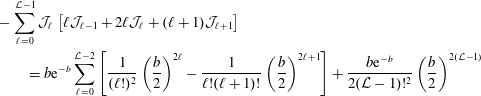 $$\begin{eqnarray}\displaystyle & & \displaystyle -\mathop{\sum }_{\ell =0}^{{\mathcal{L}}-1}{\mathcal{J}}_{\ell }\left[\ell {\mathcal{J}}_{\ell -1}+2\ell {\mathcal{J}}_{\ell }+(\ell +1){\mathcal{J}}_{\ell +1}\right]\nonumber\\ \displaystyle & & \displaystyle \qquad =b\text{e}^{-b}\mathop{\sum }_{\ell =0}^{{\mathcal{L}}-2}\left[\frac{1}{(\ell !)^{2}}\left(\frac{b}{2}\right)^{2\ell }-\frac{1}{\ell !(\ell +1)!}\left(\frac{b}{2}\right)^{2\ell +1}\right]+\frac{b\text{e}^{-b}}{2({\mathcal{L}}-1)!^{2}}\left(\frac{b}{2}\right)^{2({\mathcal{L}}-1)}\nonumber\\ \displaystyle & & \displaystyle\end{eqnarray}$$
 $$\begin{eqnarray}\displaystyle & & \displaystyle \qquad =b(\unicode[STIX]{x1D6E4}_{0}-\unicode[STIX]{x1D6E4}_{1})+O(b^{2{\mathcal{L}}-1}).\end{eqnarray}$$
This shows that in the finite ${\mathcal{L}}$
limit, Brizard’s
${\mathcal{L}}$
limit, Brizard’s $\langle \text{J}_{0}\rangle =\text{e}^{-b/2}$
accurately produces the FLR expressions that appear in dispersion relation only to order
$\langle \text{J}_{0}\rangle =\text{e}^{-b/2}$
accurately produces the FLR expressions that appear in dispersion relation only to order $2{\mathcal{L}}$
in
$2{\mathcal{L}}$
in $b$
. In figure 7 we plot the expressions from (B 11) and (B 12) for several choices of
$b$
. In figure 7 we plot the expressions from (B 11) and (B 12) for several choices of ${\mathcal{L}}$
along with the exact expressions. As expected, the approximations are valid for larger
${\mathcal{L}}$
along with the exact expressions. As expected, the approximations are valid for larger $b$
as we increase
$b$
as we increase ${\mathcal{L}}$
. Note that if we were to enforce
${\mathcal{L}}$
. Note that if we were to enforce ${\mathcal{J}}_{{\mathcal{L}}}=0$
(as we do in all terms not proportional to
${\mathcal{J}}_{{\mathcal{L}}}=0$
(as we do in all terms not proportional to $\unicode[STIX]{x1D714}_{\ast }$
when closing by truncation), the approximation to
$\unicode[STIX]{x1D714}_{\ast }$
when closing by truncation), the approximation to $b(\unicode[STIX]{x1D6E4}_{0}-\unicode[STIX]{x1D6E4}_{1})$
given by (B 12) would not have the final term on the right-hand side. This causes this expression to cross zero and become negative, which makes the critical gradient unphysical for large
$b(\unicode[STIX]{x1D6E4}_{0}-\unicode[STIX]{x1D6E4}_{1})$
given by (B 12) would not have the final term on the right-hand side. This causes this expression to cross zero and become negative, which makes the critical gradient unphysical for large $b$
and allows spurious instability.
$b$
and allows spurious instability.

Figure 7. Exact and approximate expressions for $\unicode[STIX]{x1D6E4}_{0}$
(i) and
$\unicode[STIX]{x1D6E4}_{0}$
(i) and $b(\unicode[STIX]{x1D6E4}_{0}-\unicode[STIX]{x1D6E4}_{1})$
(ii), which appear in the kinetic dispersion relation, equation (B 1). The approximations, given in (B 11) and (B 12) by taking
$b(\unicode[STIX]{x1D6E4}_{0}-\unicode[STIX]{x1D6E4}_{1})$
(ii), which appear in the kinetic dispersion relation, equation (B 1). The approximations, given in (B 11) and (B 12) by taking $\langle \text{J}_{0}\rangle =\text{e}^{-b/2}$
, are plotted for several choices of Laguerre resolution
$\langle \text{J}_{0}\rangle =\text{e}^{-b/2}$
, are plotted for several choices of Laguerre resolution ${\mathcal{L}}$
.
${\mathcal{L}}$
.


B.2 Dorland approach:
$\langle \text{J}_{0}\rangle =\unicode[STIX]{x1D6E4}_{0}^{1/2}$

Dorland’s approach of approximating $\langle \text{J}_{0}\rangle =\unicode[STIX]{x1D6E4}_{0}^{1/2}$
is better suited to the finite
$\langle \text{J}_{0}\rangle =\unicode[STIX]{x1D6E4}_{0}^{1/2}$
is better suited to the finite ${\mathcal{L}}$
case, and can be viewed as a closure of sorts for the FLR terms. While not formally accurate beyond first order in
${\mathcal{L}}$
case, and can be viewed as a closure of sorts for the FLR terms. While not formally accurate beyond first order in $b$
since
$b$
since $\unicode[STIX]{x1D6E4}_{0}^{1/2}=\text{e}^{-b/2}+O(b^{2})$
, the asymptotic behaviour at large
$\unicode[STIX]{x1D6E4}_{0}^{1/2}=\text{e}^{-b/2}+O(b^{2})$
, the asymptotic behaviour at large $b$
is much better than with
$b$
is much better than with $\langle \text{J}_{0}\rangle =\text{e}^{-b/2}$
. In figure 9 we again plot the exact and approximate expressions for
$\langle \text{J}_{0}\rangle =\text{e}^{-b/2}$
. In figure 9 we again plot the exact and approximate expressions for $\unicode[STIX]{x1D6E4}_{0}$
and
$\unicode[STIX]{x1D6E4}_{0}$
and $b(\unicode[STIX]{x1D6E4}_{0}-\unicode[STIX]{x1D6E4}_{1})$
for several choices of
$b(\unicode[STIX]{x1D6E4}_{0}-\unicode[STIX]{x1D6E4}_{1})$
for several choices of ${\mathcal{L}}$
. We also plot
${\mathcal{L}}$
. We also plot $\unicode[STIX]{x1D702}_{\text{crit}}$
in figure 10. Note that these FLR expressions are slightly different from Dorland’s, since Dorland used different FLR expressions in the quasineutrality equation than in the fluid equations.
$\unicode[STIX]{x1D702}_{\text{crit}}$
in figure 10. Note that these FLR expressions are slightly different from Dorland’s, since Dorland used different FLR expressions in the quasineutrality equation than in the fluid equations.
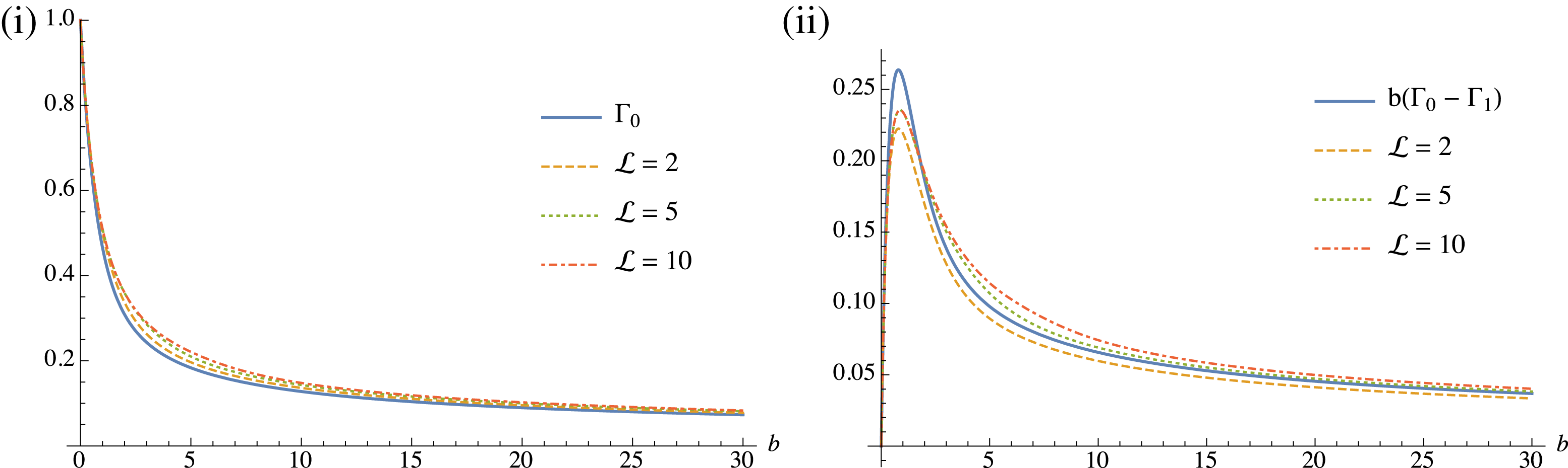
Figure 9. Exact and approximate expressions for $\unicode[STIX]{x1D6E4}_{0}$
(i) and
$\unicode[STIX]{x1D6E4}_{0}$
(i) and $b(\unicode[STIX]{x1D6E4}_{0}-\unicode[STIX]{x1D6E4}_{1})$
(ii). The approximations, using
$b(\unicode[STIX]{x1D6E4}_{0}-\unicode[STIX]{x1D6E4}_{1})$
(ii). The approximations, using $\langle \text{J}_{0}\rangle =\unicode[STIX]{x1D6E4}_{0}^{1/2}$
, are plotted for several choices of Laguerre resolution
$\langle \text{J}_{0}\rangle =\unicode[STIX]{x1D6E4}_{0}^{1/2}$
, are plotted for several choices of Laguerre resolution ${\mathcal{L}}$
. While not as accurate at small
${\mathcal{L}}$
. While not as accurate at small $b$
, the asymptotic behaviour at large
$b$
, the asymptotic behaviour at large $b$
is much better than in the
$b$
is much better than in the $\langle \text{J}_{0}\rangle =\text{e}^{-b/2}$
case shown in figure 7.
$\langle \text{J}_{0}\rangle =\text{e}^{-b/2}$
case shown in figure 7.


B.3 Other approaches
In principal, one could use any definition of $\langle \text{J}_{0}\rangle$
in the
$\langle \text{J}_{0}\rangle$
in the ${\mathcal{J}}_{\ell }$
expressions. For the purposes of free energy conservation, there are no constraints other than
${\mathcal{J}}_{\ell }$
expressions. For the purposes of free energy conservation, there are no constraints other than ${\mathcal{J}}_{{\mathcal{L}}}=0$
in the terms involving
${\mathcal{J}}_{{\mathcal{L}}}=0$
in the terms involving $H_{{\mathcal{L}},0}$
and that the same expression must be used for every
$H_{{\mathcal{L}},0}$
and that the same expression must be used for every ${\mathcal{J}}_{\ell }$
that appears in the fluid equations and quasineutrality. One would like to have at least first-order accuracy in
${\mathcal{J}}_{\ell }$
that appears in the fluid equations and quasineutrality. One would like to have at least first-order accuracy in $b$
and have reasonably behaved asymptotics for the FLR expressions that appear in the dispersion relation. Another function that satisfies these constraints is
$b$
and have reasonably behaved asymptotics for the FLR expressions that appear in the dispersion relation. Another function that satisfies these constraints is $\langle \text{J}_{0}\rangle =1/(1+b/2)$
.
$\langle \text{J}_{0}\rangle =1/(1+b/2)$
.
Appendix C. Laguerre–Hermite projection of magnetic drift terms
We first write the gyrokinetic magnetic drift term as
 $$\begin{eqnarray}\boldsymbol{v}_{d}\boldsymbol{\cdot }\unicode[STIX]{x1D735}h=(v_{\Vert }^{2}+\unicode[STIX]{x1D707}B)\text{i}\unicode[STIX]{x1D714}_{d}h=\mathop{\sum }_{\ell ,m=0}^{\infty }(v_{\Vert }^{2}+\unicode[STIX]{x1D707}B)\,\unicode[STIX]{x1D713}^{\ell }\unicode[STIX]{x1D719}^{m}\text{i}\unicode[STIX]{x1D714}_{d}\,H_{\ell ,m},\end{eqnarray}$$
where [following (Beer & Hammett Reference Beer and Hammett1996)] we have introduced the $\text{i}\unicode[STIX]{x1D714}_{d}$
operator, which combines the curvature and
$\text{i}\unicode[STIX]{x1D714}_{d}$
operator, which combines the curvature and $\unicode[STIX]{x1D735}B$
drifts into one expression, as is appropriate at low normalized plasma pressure:
$\unicode[STIX]{x1D735}B$
drifts into one expression, as is appropriate at low normalized plasma pressure:
 $$\begin{eqnarray}\text{i}\unicode[STIX]{x1D714}_{d}\equiv (1/B^{2})\hat{\boldsymbol{b}}\times \unicode[STIX]{x1D735}B\boldsymbol{\cdot }\unicode[STIX]{x1D735}.\end{eqnarray}$$
The non-dimensionalized form of this operator has the species dependencies in explicit form, $\text{i}\unicode[STIX]{x1D714}_{ds}=\text{i}\unicode[STIX]{x1D714}_{d}(\unicode[STIX]{x1D70F}_{s}/Z_{s})$
. Note that
$\text{i}\unicode[STIX]{x1D714}_{ds}=\text{i}\unicode[STIX]{x1D714}_{d}(\unicode[STIX]{x1D70F}_{s}/Z_{s})$
. Note that $\boldsymbol{v}_{d}\boldsymbol{\cdot }\unicode[STIX]{x1D735}=\boldsymbol{v}_{d}\boldsymbol{\cdot }\unicode[STIX]{x1D735}_{\bot }$
, so we can use the derivative relation from (3.15) to move the derivative operator inside the sum. We next employ the recurrence relations from (3.6) and (3.7) to express this as
$\boldsymbol{v}_{d}\boldsymbol{\cdot }\unicode[STIX]{x1D735}=\boldsymbol{v}_{d}\boldsymbol{\cdot }\unicode[STIX]{x1D735}_{\bot }$
, so we can use the derivative relation from (3.15) to move the derivative operator inside the sum. We next employ the recurrence relations from (3.6) and (3.7) to express this as
 $$\begin{eqnarray}\displaystyle & & \displaystyle \boldsymbol{v}_{d}\boldsymbol{\cdot }\unicode[STIX]{x1D735}h=\mathop{\sum }_{\ell ,m=0}^{\infty }\unicode[STIX]{x1D713}^{\ell }\left[\sqrt{(m+1)(m+2)}\unicode[STIX]{x1D719}^{m+2}+(2m+1)\unicode[STIX]{x1D719}^{m}+\sqrt{m(m-1)}\unicode[STIX]{x1D719}^{m-2}\right]\text{i}\unicode[STIX]{x1D714}_{ds}^{(\unicode[STIX]{x1D705})}H_{\ell ,m}\nonumber\\ \displaystyle & & \displaystyle \qquad +\,\mathop{\sum }_{\ell ,m=0}^{\infty }\unicode[STIX]{x1D719}^{m}\,[(\ell +1)\unicode[STIX]{x1D713}^{\ell +1}+(2\ell +1)\unicode[STIX]{x1D713}^{\ell }+\ell \unicode[STIX]{x1D713}^{\ell -1}]\text{i}\unicode[STIX]{x1D714}_{ds}^{(\unicode[STIX]{x1D735}B)}H_{\ell ,m},\end{eqnarray}$$
where we have noted how one can distinguish the roles of the $\unicode[STIX]{x1D735}B$
drift
$\unicode[STIX]{x1D735}B$
drift $\propto \unicode[STIX]{x1D714}_{ds}^{(\unicode[STIX]{x1D735}B)}$
and curvature drift
$\propto \unicode[STIX]{x1D714}_{ds}^{(\unicode[STIX]{x1D735}B)}$
and curvature drift $\propto \unicode[STIX]{x1D714}_{ds}^{(\unicode[STIX]{x1D705})}$
if one wished to make that distinction. To put this expression in the form of a Laguerre–Hermite transform, we shift the indices:
$\propto \unicode[STIX]{x1D714}_{ds}^{(\unicode[STIX]{x1D705})}$
if one wished to make that distinction. To put this expression in the form of a Laguerre–Hermite transform, we shift the indices:
 $$\begin{eqnarray}\displaystyle & & \displaystyle \boldsymbol{v}_{d}\boldsymbol{\cdot }\unicode[STIX]{x1D735}h=\mathop{\sum }_{\ell ,m=0}^{\infty }\unicode[STIX]{x1D713}^{\ell }\unicode[STIX]{x1D719}^{m}\text{i}\unicode[STIX]{x1D714}_{ds}\left[\sqrt{(m+1)(m+2)}H_{\ell ,m+2}+(\ell +1)\,H_{\ell +1,m}\right.\nonumber\\ \displaystyle & & \displaystyle \qquad \left.+\,2(\ell +m+1)H_{\ell ,m}+\sqrt{m(m-1)}H_{\ell ,m-2}+\ell H_{\ell -1,m}\right].\end{eqnarray}$$
The final step is then to use orthogonality to project this expression onto the Laguerre–Hermite basis, which is now trivial. We accomplish this by multiplying by projection functions and integrating over velocity. In non-dimensional form, the result is
 $$\begin{eqnarray}\displaystyle & & \displaystyle 2\unicode[STIX]{x03C0}\int _{-\infty }^{\infty }\text{d}v_{\Vert }\int _{0}^{\infty }\text{d}\unicode[STIX]{x1D707}\,B\unicode[STIX]{x1D713}_{\ell }\unicode[STIX]{x1D719}_{m}\boldsymbol{v}_{d}\boldsymbol{\cdot }\unicode[STIX]{x1D735}h=\text{i}\unicode[STIX]{x1D714}_{ds}\left[\sqrt{(m+1)(m+2)}\,H_{\ell ,m+2}+(\ell +1)\,H_{\ell +1,m}\right.\nonumber\\ \displaystyle & & \displaystyle \qquad \left.+\,2\,(\ell +m+1)\,H_{\ell ,m}+\sqrt{m(m-1)}\,H_{\ell ,m-2}+\ell \,H_{\ell -1,m}\right].\end{eqnarray}$$
This produces the magnetic drift terms for the $\text{d}G_{\ell ,m}/\text{d}t$
equations. The
$\text{d}G_{\ell ,m}/\text{d}t$
equations. The $v_{\Vert }^{2}$
dependence of the curvature drift couples
$v_{\Vert }^{2}$
dependence of the curvature drift couples $m$
moments to
$m$
moments to $m+2$
and
$m+2$
and $m-2$
moments, and the
$m-2$
moments, and the $\unicode[STIX]{x1D707}B$
dependence of the
$\unicode[STIX]{x1D707}B$
dependence of the $\unicode[STIX]{x1D735}B$
drift couples
$\unicode[STIX]{x1D735}B$
drift couples $\ell$
moments to
$\ell$
moments to $\ell +1$
and
$\ell +1$
and $\ell -1$
moments.
$\ell -1$
moments.
Appendix D. Pseudo-spectral alternative to Laguerre convolutions
D.1 A standard dealiased pseudo-spectral algorithm
The quadratic nonlinear terms in the gyrokinetic equation introduce convolutions into any spectral representation of the equations. This is familiar in flux-tube gyrokinetics. The standard approach is to employ a dealiased pseudo-spectral algorithm. To illustrate the approach, we consider a typical nonlinear term,
 $$\begin{eqnarray}\boldsymbol{v}_{E}\boldsymbol{\cdot }\unicode[STIX]{x1D735}n=\frac{\unicode[STIX]{x2202}\unicode[STIX]{x1D6F7}}{\unicode[STIX]{x2202}x}\frac{\unicode[STIX]{x2202}n}{\unicode[STIX]{x2202}y}-\frac{\unicode[STIX]{x2202}\unicode[STIX]{x1D6F7}}{\unicode[STIX]{x2202}y}\frac{\unicode[STIX]{x2202}n}{\unicode[STIX]{x2202}x},\end{eqnarray}$$
in which $x$
and
$x$
and $y$
are understood to be appropriately defined perpendicular field line following coordinates. Given a perpendicular coordinate-space Fourier representation of
$y$
are understood to be appropriately defined perpendicular field line following coordinates. Given a perpendicular coordinate-space Fourier representation of $\unicode[STIX]{x1D6F7}$
and
$\unicode[STIX]{x1D6F7}$
and $n$
with
$n$
with $N$
modes in each direction, one first computes the derivatives as multiplications by
$N$
modes in each direction, one first computes the derivatives as multiplications by $\text{i}k_{x}$
and
$\text{i}k_{x}$
and $\text{i}k_{y}$
. Then one uses a discrete Fourier transform to find a discretized representation of each quantity on a grid with
$\text{i}k_{y}$
. Then one uses a discrete Fourier transform to find a discretized representation of each quantity on a grid with $3N/2$
grid points in each direction. The fields are thus known on a mesh with
$3N/2$
grid points in each direction. The fields are thus known on a mesh with $9/4$
more grid points than spectral modes. The extra grid points are important in the dealiasing step.
$9/4$
more grid points than spectral modes. The extra grid points are important in the dealiasing step.
Equation (D 1) is evaluated on the higher resolution spatial grid by pointwise multiplication and addition. The result is then transformed back to the lower resolution spectral representation with an inverse discrete Fourier transform. Information contained in the high-frequency (unresolved) modes is simply discarded. Surprisingly, this ‘dealiasing’ process recovers the exact spectral convolution (Orszag Reference Orszag1971), including conservation of energy. Whether or not one should dealias is a matter of debate, but the basic idea is that dealiasing is more important as sharp derivatives appear in the solution. For smoothly varying, random fields that often characterize turbulence, dealiasing is frequently not done.
D.2 Pseudo-spectral nonlinearity in the Laguerre–Hermite representation
Relative to the example above, equation (3.19) is complicated by the convolution over Laguerre moments that is induced by finite Larmor radius effects. There is no corresponding Hermite convolution, but only because the FLR-averaged $\boldsymbol{E}\times \boldsymbol{B}$
drift corresponds to
$\boldsymbol{E}\times \boldsymbol{B}$
drift corresponds to $m=0$
in Hermite space. (An electromagnetic nonlinearity would have
$m=0$
in Hermite space. (An electromagnetic nonlinearity would have $m=1$
Hermite structure and would require a three term convolution.) At low resolution, the Laguerre convolution can be carried out without much difficulty, using (3.19)–(3.20). For more than a few Laguerre moments, it will be more efficient to use the analogue of the Fourier dealiased pseudo-spectral method. Our approach is standard and well described in Boyd (Reference Boyd2001).
$m=1$
Hermite structure and would require a three term convolution.) At low resolution, the Laguerre convolution can be carried out without much difficulty, using (3.19)–(3.20). For more than a few Laguerre moments, it will be more efficient to use the analogue of the Fourier dealiased pseudo-spectral method. Our approach is standard and well described in Boyd (Reference Boyd2001).
We seek accurate integrals of the product of three Laguerre functions, as is clear from (3.20). This implies that we must be able to integrate polynomials of degree $3({\mathcal{L}}-1)$
accurately. We will proceed by transforming to a discretized
$3({\mathcal{L}}-1)$
accurately. We will proceed by transforming to a discretized $\unicode[STIX]{x1D707}B$
grid, evaluating the nonlinear term pointwise and transforming back. To obtain spectral accuracy and avoid aliasing, we pad the
$\unicode[STIX]{x1D707}B$
grid, evaluating the nonlinear term pointwise and transforming back. To obtain spectral accuracy and avoid aliasing, we pad the $H$
arrays with zeroes in the Laguerre dimension, for
$H$
arrays with zeroes in the Laguerre dimension, for $\ell ={\mathcal{L}}$
to
$\ell ={\mathcal{L}}$
to $J-1$
. We need
$J-1$
. We need $2J-1\geqslant 3({\mathcal{L}}-1)$
, or
$2J-1\geqslant 3({\mathcal{L}}-1)$
, or $J\geqslant 3{\mathcal{L}}/2-1$
. Thus the ‘three-halves’ rule is replaced by this expression for
$J\geqslant 3{\mathcal{L}}/2-1$
. Thus the ‘three-halves’ rule is replaced by this expression for $J$
in our problem. For
$J$
in our problem. For ${\mathcal{L}}=2$
, as in the Beer–Hammett equations, there is the surprise that we do not need to dealias the Laguerre moments, but this is not true in general. Note that because our indices start from zero, there are
${\mathcal{L}}=2$
, as in the Beer–Hammett equations, there is the surprise that we do not need to dealias the Laguerre moments, but this is not true in general. Note that because our indices start from zero, there are $J$
moments and
$J$
moments and $J$
quadrature points, denoted by
$J$
quadrature points, denoted by $x_{j}=(\unicode[STIX]{x1D707}B)_{j}$
. The specific values of the
$x_{j}=(\unicode[STIX]{x1D707}B)_{j}$
. The specific values of the $x_{j}$
can be found from
$x_{j}$
can be found from $\unicode[STIX]{x1D713}_{J}(x_{j})=0$
. The weights that are used to perform integrals on this grid can be precalculated from
$\unicode[STIX]{x1D713}_{J}(x_{j})=0$
. The weights that are used to perform integrals on this grid can be precalculated from
 $$\begin{eqnarray}w_{j}=\int _{0}^{\infty }\text{d}x\,\frac{\unicode[STIX]{x1D713}^{J}(x)}{\unicode[STIX]{x1D713}_{J}^{\prime }(x_{j})(x-x_{j})}.\end{eqnarray}$$
To execute this algorithm, one would precalculate $\unicode[STIX]{x1D713}^{\ell }(x_{j})$
,
$\unicode[STIX]{x1D713}^{\ell }(x_{j})$
, $\unicode[STIX]{x1D713}_{\ell }(x_{j})$
and
$\unicode[STIX]{x1D713}_{\ell }(x_{j})$
and $w_{j}$
. These are the items required to move back and forth from the discrete
$w_{j}$
. These are the items required to move back and forth from the discrete $\unicode[STIX]{x1D707}B$
grid to the moment representation. For example, if we denote the distribution function
$\unicode[STIX]{x1D707}B$
grid to the moment representation. For example, if we denote the distribution function $h$
on the discrete
$h$
on the discrete $\unicode[STIX]{x1D707}B$
grid determined by the value of
$\unicode[STIX]{x1D707}B$
grid determined by the value of $J$
as
$J$
as $h_{J}(k_{x},k_{y},z,m,x_{j})$
, then
$h_{J}(k_{x},k_{y},z,m,x_{j})$
, then
 $$\begin{eqnarray}h_{J}(k_{x},k_{y},z,m,x_{j})=\mathop{\sum }_{\ell =0}^{{\mathcal{L}}-1}\unicode[STIX]{x1D713}^{\ell }(x_{j})H_{\ell ,m}(k_{x},k_{y},z).\end{eqnarray}$$
The sum does not need to go beyond ${\mathcal{L}}-1$
for the obvious reason that all of the
${\mathcal{L}}-1$
for the obvious reason that all of the $H_{\ell ,m}$
moments are zero in that range, but there are
$H_{\ell ,m}$
moments are zero in that range, but there are $J$
rows in this matrix, as required to obtain the values of
$J$
rows in this matrix, as required to obtain the values of $h_{J}(x_{j})$
. The inverse transform requires the
$h_{J}(x_{j})$
. The inverse transform requires the $\unicode[STIX]{x1D713}_{\ell }(x_{j})$
matrix, and the weights required for the integration,
$\unicode[STIX]{x1D713}_{\ell }(x_{j})$
matrix, and the weights required for the integration, $w_{j}$
. It is convenient to store these as one matrix,
$w_{j}$
. It is convenient to store these as one matrix, $T_{\ell j}=\unicode[STIX]{x1D713}_{\ell }(x_{j})w_{j}$
, so that
$T_{\ell j}=\unicode[STIX]{x1D713}_{\ell }(x_{j})w_{j}$
, so that
 $$\begin{eqnarray}H_{\ell ,m}(k_{x},k_{y},z)=\mathop{\sum }_{j=0}^{J-1}T_{\ell j}h_{J}(k_{x},k_{y},z,m,x_{j}).\end{eqnarray}$$
In this direction, there are $J$
columns, but only
$J$
columns, but only ${\mathcal{L}}$
rows in the transformation matrix.
${\mathcal{L}}$
rows in the transformation matrix.
This pseudo-spectral evaluation of the nonlinear term is exactly equivalent to the spectral convolution form in (3.19). The procedure will be expensive for large values of ${\mathcal{L}}$
, but not more expensive than evaluating the convolutions directly. For modest values of
${\mathcal{L}}$
, but not more expensive than evaluating the convolutions directly. For modest values of ${\mathcal{L}}$
, it is likely that the highly optimized nature of matrix-vector multiplication on our target hardware (GPUs) will make the pseudo-spectral approach inexpensive. For very small values of
${\mathcal{L}}$
, it is likely that the highly optimized nature of matrix-vector multiplication on our target hardware (GPUs) will make the pseudo-spectral approach inexpensive. For very small values of ${\mathcal{L}}$
the pseudo-spectral approach is not required: the convolutions only give a few terms, which one can evaluate by hand as was done in the Dorland, Beer and Snyder gyrofluid models.
${\mathcal{L}}$
the pseudo-spectral approach is not required: the convolutions only give a few terms, which one can evaluate by hand as was done in the Dorland, Beer and Snyder gyrofluid models.
Appendix E. Collision operator
E.1 The field–particle terms
The field–particle or integral components of $C(h)$
ensure conservation laws by construction. The real-space moments which appear in field–particle terms are expressed in Laguerre–Hermite form in (3.39)–(3.42). These scalar quantities, such as
$C(h)$
ensure conservation laws by construction. The real-space moments which appear in field–particle terms are expressed in Laguerre–Hermite form in (3.39)–(3.42). These scalar quantities, such as $\bar{u}_{\Vert }$
, determine how much of a particular quantity (such as real-space parallel momentum) needs to be restored. The coefficients of these real-space moments in the second line of (3.35) determine the velocity-space structure of the restoring terms. For example, the parallel momentum is restored with
$\bar{u}_{\Vert }$
, determine how much of a particular quantity (such as real-space parallel momentum) needs to be restored. The coefficients of these real-space moments in the second line of (3.35) determine the velocity-space structure of the restoring terms. For example, the parallel momentum is restored with $+\unicode[STIX]{x1D708}\bar{u}_{\Vert }v_{\Vert }\text{J}_{0}F_{M}$
which can be recast as
$+\unicode[STIX]{x1D708}\bar{u}_{\Vert }v_{\Vert }\text{J}_{0}F_{M}$
which can be recast as
 $$\begin{eqnarray}\unicode[STIX]{x1D708}\bar{u}_{\Vert }v_{\Vert }\text{J}_{0}F_{M}=\unicode[STIX]{x1D708}\bar{u}_{\Vert }\unicode[STIX]{x1D713}^{0}\unicode[STIX]{x1D719}^{1}\text{J}_{0}=\unicode[STIX]{x1D708}\bar{u}_{\Vert }\unicode[STIX]{x1D713}^{0}\unicode[STIX]{x1D719}^{1}\left(\mathop{\sum }_{k=0}^{\infty }\unicode[STIX]{x1D713}_{k}{\mathcal{J}}_{k}\right).\end{eqnarray}$$
Projecting this term onto the Laguerre–Hermite basis as in (C 5), we have
 $$\begin{eqnarray}2\unicode[STIX]{x03C0}\int _{-\infty }^{\infty }\text{d}v_{\Vert }\int _{0}^{\infty }\text{d}\unicode[STIX]{x1D707}\,B\unicode[STIX]{x1D713}_{\ell }\unicode[STIX]{x1D719}_{m}~\unicode[STIX]{x1D708}\bar{u}_{\Vert }\unicode[STIX]{x1D719}^{1}\unicode[STIX]{x1D713}^{0}\left(\mathop{\sum }_{k=0}^{\infty }\unicode[STIX]{x1D713}_{k}{\mathcal{J}}_{k}\right)=\unicode[STIX]{x1D708}\bar{u}_{\Vert }\unicode[STIX]{x1D6FF}_{m1}\mathop{\sum }_{k=0}^{\infty }{\mathcal{J}}_{k}\unicode[STIX]{x1D6FF}_{\ell k}=\unicode[STIX]{x1D708}\bar{u}_{\Vert }\unicode[STIX]{x1D6FF}_{m1}{\mathcal{J}}_{\ell }.\end{eqnarray}$$
Here, the finite Larmor radius average that is expressed by the Bessel function results in a convolution over the Laguerre basis, as described in (3.20). In the case of the parallel momentum, one of the Laguerre basis functions in the triple product is $\unicode[STIX]{x1D713}^{0}$
, so the convolution reduces to a simple delta function,
$\unicode[STIX]{x1D713}^{0}$
, so the convolution reduces to a simple delta function, $\unicode[STIX]{x1D6FF}_{\ell k}$
. The dependence on
$\unicode[STIX]{x1D6FF}_{\ell k}$
. The dependence on $\unicode[STIX]{x1D719}^{1}$
produces the
$\unicode[STIX]{x1D719}^{1}$
produces the $\unicode[STIX]{x1D6FF}_{m1}$
. So in the end, the parallel momentum conservation term appears in the
$\unicode[STIX]{x1D6FF}_{m1}$
. So in the end, the parallel momentum conservation term appears in the $m=1$
equations, for all values of
$m=1$
equations, for all values of $\ell$
[see (3.21)]. The rest of the conservation terms are entirely analogous.
$\ell$
[see (3.21)]. The rest of the conservation terms are entirely analogous.
The conserving terms in (3.35) manifestly maintain constant momentum and energy. The number of particles is also conserved, as is clear from the initial form of this collision operator as a divergence in velocity space. Finite Larmor radius effects obscure local number conservation, as it would appear that the leading-order term $-\unicode[STIX]{x1D708}bH_{0,0}$
represents local classical diffusion. In gyrokinetics, this term is cancelled at long wavelength by the term that enforces perpendicular momentum conservation,
$-\unicode[STIX]{x1D708}bH_{0,0}$
represents local classical diffusion. In gyrokinetics, this term is cancelled at long wavelength by the term that enforces perpendicular momentum conservation, $+\unicode[STIX]{x1D708}\sqrt{b}{\mathcal{J}}_{0}\bar{u}_{\bot }$
.
$+\unicode[STIX]{x1D708}\sqrt{b}{\mathcal{J}}_{0}\bar{u}_{\bot }$
.
Parallel momentum conservation is manifest, but it is instructive to consider the small- $b$
limit of (3.21) nonetheless, assuming no finite-
$b$
limit of (3.21) nonetheless, assuming no finite- $\ell$
fluctuations (only for clarity):
$\ell$
fluctuations (only for clarity):
 $$\begin{eqnarray}\displaystyle \frac{\text{d}G_{0,1}}{\text{d}t}+\cdots & = & \displaystyle -\unicode[STIX]{x1D708}(b+1)H_{0,1}+\unicode[STIX]{x1D708}\,{\mathcal{J}}_{0}\bar{u}_{\Vert }=-\unicode[STIX]{x1D708}(b+1)H_{0,1}+\unicode[STIX]{x1D708}\,(1-b/2)H_{0,1}\nonumber\\ \displaystyle & = & \displaystyle -\unicode[STIX]{x1D708}\frac{3b}{2}H_{0,1}+O(b^{2}).\end{eqnarray}$$
In the long wavelength limit $(b\rightarrow 0)$
, the guiding centre parallel momentum is conserved. Conservation of the real-space momentum is clear from the role of
$(b\rightarrow 0)$
, the guiding centre parallel momentum is conserved. Conservation of the real-space momentum is clear from the role of $\bar{u}_{\Vert }$
.
$\bar{u}_{\Vert }$
.
We have chosen the orthonormal form of the probabilists’ Hermite polynomials. This slightly obscures energy conservation, because of the factor of $1/\sqrt{m!}$
in the
$1/\sqrt{m!}$
in the $m=2$
equation. That is,
$m=2$
equation. That is, $T_{\Vert }=\sqrt{2}G_{0,2}$
. To see that energy is conserved in the long wavelength limit, we consider the effect of collisions on the total guiding centre temperature
$T_{\Vert }=\sqrt{2}G_{0,2}$
. To see that energy is conserved in the long wavelength limit, we consider the effect of collisions on the total guiding centre temperature $T=(T_{\Vert }+2T_{\bot })/3$
and take the
$T=(T_{\Vert }+2T_{\bot })/3$
and take the $b\rightarrow 0$
limit:
$b\rightarrow 0$
limit:
 $$\begin{eqnarray}\displaystyle \frac{\text{d}T}{\text{d}t} & = & \displaystyle \frac{1}{3}\left(\sqrt{2}\frac{\text{d}G_{0,2}}{\text{d}t}+2\frac{\text{d}G_{1,0}}{\text{d}t}\right)+\cdots \nonumber\\ \displaystyle & = & \displaystyle -\frac{\unicode[STIX]{x1D708}}{3}(b+2)\sqrt{2}H_{0,2}+\frac{2\unicode[STIX]{x1D708}}{3}T-\frac{2\unicode[STIX]{x1D708}}{3}(b+2)H_{1,0}\nonumber\\ \displaystyle & & \displaystyle +\,\frac{2\unicode[STIX]{x1D708}}{3}b(H_{0,0}+H_{1,0})-\frac{4\unicode[STIX]{x1D708}}{3}\frac{b}{2}T+\frac{4\unicode[STIX]{x1D708}}{3}H_{1,0}\nonumber\\ \displaystyle & \simeq & \displaystyle -\frac{2\unicode[STIX]{x1D708}}{3}T_{\Vert }+2\unicode[STIX]{x1D708}T-\frac{4\unicode[STIX]{x1D708}}{3}T_{\bot }\nonumber\\ \displaystyle & = & \displaystyle 2\unicode[STIX]{x1D708}\left[T-\frac{T_{\Vert }+2T_{\bot }}{3}\right]=0.\end{eqnarray}$$
E.2 Collisions and free energy
The collision operator will not increase the free energy as long as the right-hand side of (4.10) is non-positive. By construction, $\unicode[STIX]{x2202}W_{C}/\unicode[STIX]{x2202}t=0$
for any perturbation that is Maxwellian in real space. In the previous section we demonstrated conservation of number, parallel momentum and energy in the
$\unicode[STIX]{x2202}W_{C}/\unicode[STIX]{x2202}t=0$
for any perturbation that is Maxwellian in real space. In the previous section we demonstrated conservation of number, parallel momentum and energy in the $b\rightarrow 0$
limit. That is,
$b\rightarrow 0$
limit. That is,
 $$\begin{eqnarray}\displaystyle & & \displaystyle \frac{1}{\unicode[STIX]{x1D708}\unicode[STIX]{x1D70F}_{s}}\frac{\unicode[STIX]{x2202}W_{C}}{\unicode[STIX]{x2202}t}|_{\text{fluid}}\equiv -b|H_{0,0}|^{2}-|H_{0,1}|^{2}-2|H_{0,2}|^{2}-2|H_{1,0}|^{2}+|\bar{u}_{\Vert }|^{2}+|\bar{u}_{\bot }|^{2}+3|\bar{T}|^{2}\nonumber\\ \displaystyle & & \displaystyle \qquad =-b|H_{0,0}|^{2}-|H_{0,1}|^{2}-2|H_{0,2}|^{2}-2|H_{1,0}|^{2}+|H_{0,1}|^{2}+b|H_{0,0}|^{2}+\frac{1}{3}(T_{\Vert }+2T_{\bot })^{2}\nonumber\\ \displaystyle & & \displaystyle \qquad =-2|H_{0,2}|^{2}-2|H_{1,0}|^{2}+\frac{1}{3}|\sqrt{2}H_{0,2}+2H_{1,0}|^{2}\nonumber\\ \displaystyle & & \displaystyle \qquad \leqslant 0.\end{eqnarray}$$
The triangle inequality was used to obtain the final result. Equality is obtained when the fluctuations in free energy are Maxwellian,
 $$\begin{eqnarray}T={\textstyle \frac{1}{3}}(T_{\Vert }+2T_{\bot })={\textstyle \frac{1}{3}}(\sqrt{2}H_{0,2}+2H_{1,0}).\end{eqnarray}$$
Upon enforcing this constraint and eliminating $H_{1,0}$
from
$H_{1,0}$
from ${\dot{W}}_{C}$
by setting
${\dot{W}}_{C}$
by setting
 $$\begin{eqnarray}H_{1,0}={\textstyle \frac{1}{2}}(3T-\sqrt{2}H_{0,2})\end{eqnarray}$$
so that
 $$\begin{eqnarray}|H_{1,0}|^{2}={\textstyle \frac{1}{4}}(9|T|^{2}-6\sqrt{2}H_{0,2}T+2|H_{0,2}|^{2}),\end{eqnarray}$$
one finds
 $$\begin{eqnarray}\frac{1}{\unicode[STIX]{x1D708}\unicode[STIX]{x1D70F}_{s}}\frac{\unicode[STIX]{x2202}W_{C}}{\unicode[STIX]{x2202}t}|_{\text{Maxwellian}}\equiv -2|H_{0,2}|^{2}-\frac{1}{2}(9|T|^{2}-6\sqrt{2}H_{0,2}T+2|H_{0,2}|^{2})+3|T|^{2}=0.\end{eqnarray}$$
As advertised, the right-hand side vanishes when $\sqrt{2}H_{0,2}=T=T_{\Vert }=T_{\bot }$
. Fluctuations that are Maxwellian (with a single temperature) are not affected by collisions.
$\sqrt{2}H_{0,2}=T=T_{\Vert }=T_{\bot }$
. Fluctuations that are Maxwellian (with a single temperature) are not affected by collisions.
The form of the ${\mathcal{J}}_{\ell }$
operator ensures that the FLR corrections to real-space quantities such as
${\mathcal{J}}_{\ell }$
operator ensures that the FLR corrections to real-space quantities such as $\bar{u}_{\Vert }$
are strictly sub-dominant, as can be shown by rearranging the terms the expression for
$\bar{u}_{\Vert }$
are strictly sub-dominant, as can be shown by rearranging the terms the expression for ${\dot{W}}_{C}$
, but the existence of an
${\dot{W}}_{C}$
, but the existence of an $H$
-theorem is more easily shown before gyroaveraging, as we demonstrate in the following section.
$H$
-theorem is more easily shown before gyroaveraging, as we demonstrate in the following section.
To summarize, we have demonstrated that long wavelength, real-space fluctuations of density, momentum and temperature are unaffected by collisions in our model. In fact, the conservation laws for real space density, momentum and energy are correctly implemented at all wavelengths. Small-scale fluctuations of guiding centre density, momentum and energy are not locally conserved. This is the correct physical behaviour. For example, a collision at some position $\boldsymbol{r}$
in general causes an instantaneous change in the density of guiding centres at some potentially distant
$\boldsymbol{r}$
in general causes an instantaneous change in the density of guiding centres at some potentially distant $\boldsymbol{R}$
in gyrokinetics. Of course, it actually takes a gyroperiod to establish the new gyrocentre, but one averages over that fast time scale in developing the gyrokinetic equations.
$\boldsymbol{R}$
in gyrokinetics. Of course, it actually takes a gyroperiod to establish the new gyrocentre, but one averages over that fast time scale in developing the gyrokinetic equations.
For all other (non-Maxwellian in real space) fluctuations, the free energy of this gyrokinetic model is strictly damped by collisions. Pitch angle and energy scattering both contribute to this damping.
E.3 The H-theorem
We began with the Dougherty collision operator, which was shown in § 3.5 to be
 $$\begin{eqnarray}C(h)=\unicode[STIX]{x1D708}\frac{\unicode[STIX]{x2202}}{\unicode[STIX]{x2202}\boldsymbol{v}}\boldsymbol{\cdot }\left[\frac{T_{0}}{M}\frac{\unicode[STIX]{x2202}h}{\unicode[STIX]{x2202}\boldsymbol{v}}+\frac{\unicode[STIX]{x1D6FF}T}{M}\frac{\unicode[STIX]{x2202}F_{M}}{\unicode[STIX]{x2202}\boldsymbol{v}}+\boldsymbol{v}\,h-\unicode[STIX]{x1D6FF}\boldsymbol{u}\,F_{M}\right].\end{eqnarray}$$
Note that in this section we work with dimensional, non-normalized quantities. Here we have $n_{0}\unicode[STIX]{x1D6FF}\boldsymbol{u}=\int \text{d}^{3}\boldsymbol{v}\,\boldsymbol{v}h$
and
$n_{0}\unicode[STIX]{x1D6FF}\boldsymbol{u}=\int \text{d}^{3}\boldsymbol{v}\,\boldsymbol{v}h$
and $n_{0}\unicode[STIX]{x1D6FF}T=\int \text{d}^{3}\boldsymbol{v}\,(mv^{2}/3-T_{0})h$
. An equivalent form of
$n_{0}\unicode[STIX]{x1D6FF}T=\int \text{d}^{3}\boldsymbol{v}\,(mv^{2}/3-T_{0})h$
. An equivalent form of $C$
is
$C$
is
 $$\begin{eqnarray}C(h)=\unicode[STIX]{x1D708}\frac{\unicode[STIX]{x2202}}{\unicode[STIX]{x2202}\boldsymbol{v}}\boldsymbol{\cdot }\left[\frac{T_{0}}{M}F_{M}\frac{\unicode[STIX]{x2202}}{\unicode[STIX]{x2202}\boldsymbol{v}}\left(\frac{h}{F_{M}}-\frac{Mv^{2}}{2T_{0}}\frac{\unicode[STIX]{x1D6FF}T}{T_{0}}-\frac{M}{T_{0}}\boldsymbol{v}\boldsymbol{\cdot }\unicode[STIX]{x1D6FF}\boldsymbol{u}\right)\right].\end{eqnarray}$$
The entropy production rate is
 $$\begin{eqnarray}\frac{\text{d}S}{\text{d}t}=-\int \text{d}^{3}\boldsymbol{v}\,\frac{h}{F_{M}}C(h).\end{eqnarray}$$
By construction, we have
 $$\begin{eqnarray}\int \text{d}^{3}\boldsymbol{v}\,\boldsymbol{v}C(h)=0\quad \text{and}\quad \int \text{d}^{3}\boldsymbol{v}\,v^{2}C(h)=0,\end{eqnarray}$$
so we are free to modify (E 12) as follows:
 $$\begin{eqnarray}\frac{\text{d}S}{\text{d}t}=-\int \text{d}^{3}\boldsymbol{v}\left(\frac{h}{F_{M}}-\frac{Mv^{2}}{2T_{0}}\frac{\unicode[STIX]{x1D6FF}T}{T_{0}}-\frac{M}{T_{0}}\boldsymbol{v}\boldsymbol{\cdot }\unicode[STIX]{x1D6FF}\boldsymbol{u}\right)C(h).\end{eqnarray}$$
Inserting $C(h)$
from (E 11), we can then integrate by parts to find
$C(h)$
from (E 11), we can then integrate by parts to find
 $$\begin{eqnarray}\frac{\text{d}S}{\text{d}t}=\unicode[STIX]{x1D708}\frac{T_{0}}{M}\int \text{d}^{3}\boldsymbol{v}\,F_{M}\left|\frac{\unicode[STIX]{x2202}}{\unicode[STIX]{x2202}\boldsymbol{v}}\left(\frac{h}{F_{M}}-\frac{Mv^{2}}{2T_{0}}\frac{\unicode[STIX]{x1D6FF}T}{T_{0}}-\frac{M}{T_{0}}\boldsymbol{v}\boldsymbol{\cdot }\unicode[STIX]{x1D6FF}\boldsymbol{u}\right)\right|^{2}.\end{eqnarray}$$
In this form, it can be seen that ${\dot{S}}\geqslant 0$
. To obtain
${\dot{S}}\geqslant 0$
. To obtain ${\dot{S}}=0$
, it must be the case that
${\dot{S}}=0$
, it must be the case that
 $$\begin{eqnarray}\frac{\unicode[STIX]{x2202}}{\unicode[STIX]{x2202}\boldsymbol{v}}\left(\frac{h}{F_{M}}-\frac{Mv^{2}}{2T_{0}}\frac{\unicode[STIX]{x1D6FF}T}{T_{0}}-\frac{M}{T_{0}}\boldsymbol{v}\boldsymbol{\cdot }\unicode[STIX]{x1D6FF}\boldsymbol{u}\right)=0\end{eqnarray}$$
for all $\boldsymbol{v}$
, which implies
$\boldsymbol{v}$
, which implies
 $$\begin{eqnarray}\frac{h}{F_{M}}-\frac{Mv^{2}}{2T_{0}}\frac{\unicode[STIX]{x1D6FF}T}{T_{0}}-\frac{M}{T_{0}}\boldsymbol{v}\boldsymbol{\cdot }\unicode[STIX]{x1D6FF}\boldsymbol{u}=\unicode[STIX]{x1D6FC},\end{eqnarray}$$
where $\unicode[STIX]{x1D6FC}$
is the integration constant. This can be rearranged to show
$\unicode[STIX]{x1D6FC}$
is the integration constant. This can be rearranged to show
 $$\begin{eqnarray}h=\unicode[STIX]{x1D6FC}F_{M}+\boldsymbol{v}\boldsymbol{\cdot }\unicode[STIX]{x1D6FF}\boldsymbol{u}F_{M}\frac{M}{T_{0}}+F_{M}\frac{Mv^{2}}{2T_{0}}\frac{\unicode[STIX]{x1D6FF}T}{T_{0}},\end{eqnarray}$$
from which one can immediately conclude that ${\dot{S}}=0$
if and only if
${\dot{S}}=0$
if and only if $h$
is a perturbed Maxwellian.
$h$
is a perturbed Maxwellian.
The Dougherty collision operator (together with our gyroaveraged version) is also self-adjoint. A third equivalent form of (E 11) is
 $$\begin{eqnarray}C(h)=\unicode[STIX]{x1D708}\frac{\unicode[STIX]{x2202}}{\unicode[STIX]{x2202}\boldsymbol{v}}\boldsymbol{\cdot }\left[\frac{T_{0}}{M}F_{M}\frac{\unicode[STIX]{x2202}}{\unicode[STIX]{x2202}\boldsymbol{v}}\left(\frac{h}{F_{M}}\right)-\frac{\unicode[STIX]{x1D6FF}T}{T_{0}}F_{M}\boldsymbol{v}-F_{M}\unicode[STIX]{x1D6FF}\boldsymbol{u}\right].\end{eqnarray}$$
We consider the expression
 $$\begin{eqnarray}\int \text{d}^{3}\boldsymbol{v}\,\frac{h_{a}}{F_{M}}C(h_{b})\end{eqnarray}$$
for any two distribution functions $h_{a}$
and
$h_{a}$
and $h_{b}$
. One can write
$h_{b}$
. One can write
 $$\begin{eqnarray}\displaystyle \int \text{d}^{3}\boldsymbol{v}\,\frac{h_{a}}{F_{M}}C(h_{b}) & = & \displaystyle \unicode[STIX]{x1D708}\int \text{d}^{3}\boldsymbol{v}\,\frac{h_{a}}{f_{M}}\frac{\unicode[STIX]{x2202}}{\unicode[STIX]{x2202}\boldsymbol{v}}\boldsymbol{\cdot }\left[\frac{T_{0}}{M}F_{M}\frac{\unicode[STIX]{x2202}}{\unicode[STIX]{x2202}\boldsymbol{v}}\left(\frac{h_{b}}{F_{M}}\right)-\frac{\unicode[STIX]{x1D6FF}T}{T_{0}}F_{M}\boldsymbol{v}-F_{M}\unicode[STIX]{x1D6FF}\boldsymbol{u}\right]\nonumber\\ \displaystyle & = & \displaystyle \unicode[STIX]{x1D708}\int \text{d}^{3}\boldsymbol{v}\,\frac{h_{a}}{F_{M}}\frac{\unicode[STIX]{x2202}}{\unicode[STIX]{x2202}\boldsymbol{v}}\left[\frac{T_{0}}{m}F_{M}\frac{\unicode[STIX]{x2202}}{\unicode[STIX]{x2202}\boldsymbol{v}}\left(\frac{h_{b}}{F_{M}}\right)\right]-\unicode[STIX]{x1D708}\frac{\unicode[STIX]{x1D6FF}T}{T_{0}}\int \text{d}^{3}\boldsymbol{v}\frac{h_{a}}{F_{M}}\frac{\unicode[STIX]{x2202}}{\unicode[STIX]{x2202}\boldsymbol{v}}\boldsymbol{\cdot }\left(F_{M}\boldsymbol{v}\right)\nonumber\\ \displaystyle & & \displaystyle -\,\unicode[STIX]{x1D708}\unicode[STIX]{x1D6FF}\boldsymbol{u}\boldsymbol{\cdot }\left(\int \text{d}^{3}\boldsymbol{v}\,\frac{h_{a}}{F_{M}}\frac{\unicode[STIX]{x2202}F_{M}}{\unicode[STIX]{x2202}\boldsymbol{v}}\right)\nonumber\\ \displaystyle & = & \displaystyle \unicode[STIX]{x1D708}\int \text{d}^{3}\boldsymbol{v}\,\frac{h_{a}}{F_{M}}\frac{\unicode[STIX]{x2202}}{\unicode[STIX]{x2202}\boldsymbol{v}}\left[\frac{T_{0}}{M}F_{M}\frac{\unicode[STIX]{x2202}}{\unicode[STIX]{x2202}\boldsymbol{v}}\left(\frac{h_{b}}{F_{M}}\right)\right]-\unicode[STIX]{x1D708}\frac{\unicode[STIX]{x1D6FF}T}{T_{0}}\int \text{d}^{3}\boldsymbol{v}\,h_{a}\left(3-\frac{Mv^{2}}{T_{0}}\right)\nonumber\\ \displaystyle & & \displaystyle +\,\unicode[STIX]{x1D708}\frac{M}{T_{0}}\unicode[STIX]{x1D6FF}\boldsymbol{u}\boldsymbol{\cdot }\int \text{d}^{3}\boldsymbol{v}\,h_{a}\boldsymbol{v}.\end{eqnarray}$$
One can then integrate the first term by parts to find
 $$\begin{eqnarray}\displaystyle \int \text{d}^{3}\boldsymbol{v}\,\frac{h_{a}}{F_{M}}C(h_{b}) & = & \displaystyle -\unicode[STIX]{x1D708}\frac{T_{0}}{M}\int \text{d}^{3}\boldsymbol{v}\,F_{M}\left(\frac{\unicode[STIX]{x2202}}{\unicode[STIX]{x2202}\boldsymbol{v}}\frac{h_{a}}{F_{M}}\right)\boldsymbol{\cdot }\left(\frac{\unicode[STIX]{x2202}}{\unicode[STIX]{x2202}\boldsymbol{v}}\frac{h_{b}}{F_{M}}\right)\nonumber\\ \displaystyle & & \displaystyle +\,\frac{\unicode[STIX]{x1D708}}{3n_{0}}\left[\int \text{d}^{3}\boldsymbol{v}\,h_{b}\left(\frac{Mv^{2}}{T_{0}}-3\right)\right]\left[\int \text{d}^{3}\boldsymbol{v}\,h_{a}\left(\frac{Mv^{2}}{T_{0}}-3\right)\right]\nonumber\\ \displaystyle & & \displaystyle +\,\frac{\unicode[STIX]{x1D708}M}{n_{0}T_{0}}\left(\int \text{d}^{3}\boldsymbol{v}\,h_{b}\boldsymbol{v}\right)\boldsymbol{\cdot }\left(\int \text{d}^{3}\boldsymbol{v}\,h_{a}\boldsymbol{v}\right).\end{eqnarray}$$
This expression is completely symmetric with respect to $h_{a}$
and
$h_{a}$
and $h_{b}$
, which implies
$h_{b}$
, which implies
 $$\begin{eqnarray}\int \text{d}^{3}\boldsymbol{v}\,\frac{h_{a}}{F_{M}}C(h_{b})=\int \text{d}^{3}\boldsymbol{v}\,\frac{h_{b}}{F_{M}}C(h_{a}),\end{eqnarray}$$
i.e. the collision operator is self-adjoint. Neither gyroaveraging nor projecting onto the Laguerre–Hermite basis alters these conclusions.
Appendix F. Reproducing the Beer
$4+2$
toroidal gyrofluid model

We can reproduce the six moment ( $4+2$
) toroidal gyrofluid equation set of Beer & Hammett (Reference Beer and Hammett1996) by first truncating all moments with
$4+2$
) toroidal gyrofluid equation set of Beer & Hammett (Reference Beer and Hammett1996) by first truncating all moments with $2\ell +m>3$
. This effectively keeps all moments up to order
$2\ell +m>3$
. This effectively keeps all moments up to order $v^{3}$
. As described above, the evolution equations for the kept moments couple to higher unevolved moments via parallel convection, curvature and
$v^{3}$
. As described above, the evolution equations for the kept moments couple to higher unevolved moments via parallel convection, curvature and $\unicode[STIX]{x1D735}B$
drifts and mirror terms. For the parallel convection terms, unevolved moments in the
$\unicode[STIX]{x1D735}B$
drifts and mirror terms. For the parallel convection terms, unevolved moments in the $G_{0,3}$
and
$G_{0,3}$
and $G_{1,1}$
equations are closed using the Landau damping closures of Hammett & Perkins (Reference Hammett and Perkins1990), Dorland & Hammett (Reference Dorland and Hammett1993), which corresponds to
$G_{1,1}$
equations are closed using the Landau damping closures of Hammett & Perkins (Reference Hammett and Perkins1990), Dorland & Hammett (Reference Dorland and Hammett1993), which corresponds to
 $$\begin{eqnarray}\displaystyle & \displaystyle 2\unicode[STIX]{x1D735}_{\Vert }G_{0,4}=\frac{\unicode[STIX]{x1D6FD}_{\Vert }}{\sqrt{3}}\unicode[STIX]{x1D735}_{\Vert }G_{0,2}+\sqrt{2}D_{\Vert }|k_{\Vert }|G_{0,3}, & \displaystyle\end{eqnarray}$$
 $$\begin{eqnarray}\displaystyle & \displaystyle \sqrt{2}\unicode[STIX]{x1D735}_{\Vert }G_{1,2}=\sqrt{2}D_{\bot }|k_{\Vert }|G_{1,1}, & \displaystyle\end{eqnarray}$$
where $\unicode[STIX]{x1D6FD}_{\Vert }=(32-9\unicode[STIX]{x03C0})/(3\unicode[STIX]{x03C0}-8)$
,
$\unicode[STIX]{x1D6FD}_{\Vert }=(32-9\unicode[STIX]{x03C0})/(3\unicode[STIX]{x03C0}-8)$
, $D_{\Vert }=2\sqrt{\unicode[STIX]{x03C0}}/(3\unicode[STIX]{x03C0}-8)$
, and
$D_{\Vert }=2\sqrt{\unicode[STIX]{x03C0}}/(3\unicode[STIX]{x03C0}-8)$
, and $D_{\bot }=\sqrt{\unicode[STIX]{x03C0}}/2$
as in Dorland & Hammett (Reference Dorland and Hammett1993). For the toroidal drift terms, unevolved moments in the
$D_{\bot }=\sqrt{\unicode[STIX]{x03C0}}/2$
as in Dorland & Hammett (Reference Dorland and Hammett1993). For the toroidal drift terms, unevolved moments in the $G_{0,2}$
,
$G_{0,2}$
, $G_{1,0}$
,
$G_{1,0}$
, $G_{0,3}$
and
$G_{0,3}$
and $G_{1,1}$
equations are closed using the toroidal closures developed by Beer & Hammett (Reference Beer and Hammett1996), where closure coefficients were fit numerically so that the toroidal response function for the fluid equations matched the kinetic response. Beer’s closure corresponds to
$G_{1,1}$
equations are closed using the toroidal closures developed by Beer & Hammett (Reference Beer and Hammett1996), where closure coefficients were fit numerically so that the toroidal response function for the fluid equations matched the kinetic response. Beer’s closure corresponds to
 $$\begin{eqnarray}\displaystyle & \displaystyle \text{i}\unicode[STIX]{x1D714}_{d}(\sqrt{12}G_{0,4}+G_{1,2})=\sqrt{2}|\unicode[STIX]{x1D714}_{d}|(\unicode[STIX]{x1D708}_{1}\sqrt{2}G_{0,2}+\unicode[STIX]{x1D708}_{2}G_{1,0}), & \displaystyle\end{eqnarray}$$
 $$\begin{eqnarray}\displaystyle & \displaystyle \text{i}\unicode[STIX]{x1D714}_{d}(\sqrt{2}G_{1,2}+2G_{2,0})=2|\unicode[STIX]{x1D714}_{d}|(\unicode[STIX]{x1D708}_{3}\sqrt{2}G_{0,2}+\unicode[STIX]{x1D708}_{4}G_{1,0}), & \displaystyle\end{eqnarray}$$
 $$\begin{eqnarray}\displaystyle & \displaystyle \text{i}\unicode[STIX]{x1D714}_{d}(\sqrt{20}G_{0,5}+G_{1,3})=\frac{1}{\sqrt{6}}|\unicode[STIX]{x1D714}_{d}|(\unicode[STIX]{x1D708}_{5}G_{0,1}+\unicode[STIX]{x1D708}_{6}^{\prime }\sqrt{6}G_{0,3}+\unicode[STIX]{x1D708}_{7}^{\prime }G_{1,1}), & \displaystyle\end{eqnarray}$$
 $$\begin{eqnarray}\displaystyle & \displaystyle \text{i}\unicode[STIX]{x1D714}_{d}(\sqrt{6}G_{1,3}+2G_{2,1})=|\unicode[STIX]{x1D714}_{d}|(\unicode[STIX]{x1D708}_{8}G_{0,1}+\unicode[STIX]{x1D708}_{9}^{\prime }\sqrt{6}G_{0,3}+\unicode[STIX]{x1D708}_{10}^{\prime }G_{1,1}), & \displaystyle\end{eqnarray}$$
where $\unicode[STIX]{x1D708}_{1}-\unicode[STIX]{x1D708}_{10}$
are the closure coefficients defined in Beer & Hammett (Reference Beer and Hammett1996), and
$\unicode[STIX]{x1D708}_{1}-\unicode[STIX]{x1D708}_{10}$
are the closure coefficients defined in Beer & Hammett (Reference Beer and Hammett1996), and $\unicode[STIX]{x1D708}_{6}^{\prime }=(\unicode[STIX]{x1D708}_{6r},\unicode[STIX]{x1D708}_{6i}-11)$
,
$\unicode[STIX]{x1D708}_{6}^{\prime }=(\unicode[STIX]{x1D708}_{6r},\unicode[STIX]{x1D708}_{6i}-11)$
, $\unicode[STIX]{x1D708}_{7}^{\prime }=(\unicode[STIX]{x1D708}_{7r},\unicode[STIX]{x1D708}_{7i}-3)$
,
$\unicode[STIX]{x1D708}_{7}^{\prime }=(\unicode[STIX]{x1D708}_{7r},\unicode[STIX]{x1D708}_{7i}-3)$
, $\unicode[STIX]{x1D708}_{9}^{\prime }=(\unicode[STIX]{x1D708}_{9r},\unicode[STIX]{x1D708}_{9i}-1)$
and
$\unicode[STIX]{x1D708}_{9}^{\prime }=(\unicode[STIX]{x1D708}_{9r},\unicode[STIX]{x1D708}_{9i}-1)$
and $\unicode[STIX]{x1D708}_{10}^{\prime }=(\unicode[STIX]{x1D708}_{10r},\unicode[STIX]{x1D708}_{10i}-7)$
. The modifications of these closure coefficients are related to differences in the definitions of the higher moments here compared to Beer. This is discussed in appendix G. The critical part is that in practice, these modified coefficients give exactly the same toroidal terms as in Beer. For the mirror terms, unevolved moments in the
$\unicode[STIX]{x1D708}_{10}^{\prime }=(\unicode[STIX]{x1D708}_{10r},\unicode[STIX]{x1D708}_{10i}-7)$
. The modifications of these closure coefficients are related to differences in the definitions of the higher moments here compared to Beer. This is discussed in appendix G. The critical part is that in practice, these modified coefficients give exactly the same toroidal terms as in Beer. For the mirror terms, unevolved moments in the $G_{0,3}$
and
$G_{0,3}$
and $G_{1,1}$
equations are closed as in Beer with ‘Maxwellian’ closures since these terms introduce no new dissipative processes; this corresponds to
$G_{1,1}$
equations are closed as in Beer with ‘Maxwellian’ closures since these terms introduce no new dissipative processes; this corresponds to
 $$\begin{eqnarray}G_{0,4}\unicode[STIX]{x1D735}_{\Vert }\ln B=G_{1,2}\unicode[STIX]{x1D735}_{\Vert }\ln B=G_{2,0}\unicode[STIX]{x1D735}_{\Vert }\ln B=0.\end{eqnarray}$$
For details about what is meant by a ‘Maxwellian’ closure in our Laguerre–Hermite context, we again defer to appendix G.
Finally, the FLR expressions in Beer’s model followed the Dorland approach from appendix B, so we define the ${\mathcal{J}}_{\ell }$
operator with
${\mathcal{J}}_{\ell }$
operator with $\langle \text{J}_{0}\rangle =\unicode[STIX]{x1D6E4}_{0}^{1/2}$
and we do not fix
$\langle \text{J}_{0}\rangle =\unicode[STIX]{x1D6E4}_{0}^{1/2}$
and we do not fix ${\mathcal{J}}_{{\mathcal{L}}}=0$
. We must also change the definition of the non-Boltzmann part of the particle space density, equation (3.23), to match Beer’s approximation:
${\mathcal{J}}_{{\mathcal{L}}}=0$
. We must also change the definition of the non-Boltzmann part of the particle space density, equation (3.23), to match Beer’s approximation:
 $$\begin{eqnarray}\hat{\bar{n}}=\frac{1}{1+b/2}G_{0,0}-\frac{b/2}{(1+b/2)^{2}}G_{1,0}+\unicode[STIX]{x1D6E4}_{0}\unicode[STIX]{x1D6F7},\end{eqnarray}$$
where the $\unicode[STIX]{x1D6F7}$
term results from our definition of the particle space density as an integral involving
$\unicode[STIX]{x1D6F7}$
term results from our definition of the particle space density as an integral involving $h$
, not
$h$
, not $g$
. Thus by truncating our Laguerre–Hermite moments to keep only moments up to order
$g$
. Thus by truncating our Laguerre–Hermite moments to keep only moments up to order $v^{3}$
and choosing the above closures consistent with Beer’s closures, we can reproduce the Beer
$v^{3}$
and choosing the above closures consistent with Beer’s closures, we can reproduce the Beer $4+2$
toroidal gyrofluid model.
$4+2$
toroidal gyrofluid model.
Appendix G. Fixing non-orthogonality of Beer’s moment definitions and closures
Our Laguerre–Hermite moment definitions are generally consistent with Beer’s moment definitions, as indicated by (3.13). However, a difference arises in the definition of the higher, unresolved moments, due to the fact that our Laguerre–Hermite moments are defined to be orthogonal while Beer’s were not. For example, Beer defined
 $$\begin{eqnarray}r_{\Vert ,\Vert }=\int \text{d}^{3}\boldsymbol{v}\,v_{\Vert }^{4}g.\end{eqnarray}$$
Inserting our distribution function expansion (3.10) into this integral, we find
 $$\begin{eqnarray}r_{\Vert ,\Vert }=\sqrt{12}G_{0,4}+3G_{0,0}+6\sqrt{2}G_{0,2}=\sqrt{12}G_{0,4}+3n+6T_{\Vert }=\sqrt{12}G_{0,4}+r_{\Vert ,\Vert M}.\end{eqnarray}$$
Here $r_{\Vert ,\Vert M}=3n+6T_{\Vert }$
is ‘the Maxwellian part of the
$r_{\Vert ,\Vert M}=3n+6T_{\Vert }$
is ‘the Maxwellian part of the $r_{\Vert ,\Vert }$
moment’ in Beer’s terminology, since this expression can be calculated by taking
$r_{\Vert ,\Vert }$
moment’ in Beer’s terminology, since this expression can be calculated by taking $g$
to be purely Maxwellian in the integral. Beer’s full result for
$g$
to be purely Maxwellian in the integral. Beer’s full result for $r_{\Vert ,\Vert }$
is thus
$r_{\Vert ,\Vert }$
is thus
 $$\begin{eqnarray}r_{\Vert ,\Vert }=3n+6T_{\Vert }+\unicode[STIX]{x1D6FF}r_{\Vert ,\Vert };\end{eqnarray}$$
in this case, therefore, $\unicode[STIX]{x1D6FF}r_{\Vert ,\Vert }=\sqrt{12}G_{0,4}$
is the quantity to be evolved or closed in some fashion.
$\unicode[STIX]{x1D6FF}r_{\Vert ,\Vert }=\sqrt{12}G_{0,4}$
is the quantity to be evolved or closed in some fashion.
Now we make a subtle change in reasoning. Instead of conceptualizing some high moment in terms of Maxwellian and non-Maxwellian parts, the $r_{\Vert ,\Vert M}$
terms are better understood as the components of
$r_{\Vert ,\Vert M}$
terms are better understood as the components of $r_{\Vert ,\Vert }$
that are not orthogonal to the other moments (namely
$r_{\Vert ,\Vert }$
that are not orthogonal to the other moments (namely $n$
and
$n$
and $T_{\Vert }$
). While this difference does not change the results for even moments such as
$T_{\Vert }$
). While this difference does not change the results for even moments such as $r$
, differences do appear for odd moments. Consider, for example, the
$r$
, differences do appear for odd moments. Consider, for example, the $s_{\Vert ,\Vert }$
moment,
$s_{\Vert ,\Vert }$
moment,
 $$\begin{eqnarray}s_{\Vert ,\Vert }=\int \text{d}^{3}\boldsymbol{v}\,v_{\Vert }^{5}~g.\end{eqnarray}$$
Inserting (3.10) for $g$
and integrating gives
$g$
and integrating gives
 $$\begin{eqnarray}s_{\Vert ,\Vert }=10\sqrt{6}G_{0,3}+\sqrt{120}G_{0,5}=10q_{\Vert }+\sqrt{120}G_{0,5},\end{eqnarray}$$
where $q_{\Vert }$
appears because
$q_{\Vert }$
appears because $s_{\Vert ,\Vert }$
is not orthogonal to the lower moments. However, upon inserting a Maxwellian for
$s_{\Vert ,\Vert }$
is not orthogonal to the lower moments. However, upon inserting a Maxwellian for $g$
, Beer calculated
$g$
, Beer calculated $s_{\Vert ,\Vert M}=0$
, and thus missed the non-orthogonal part of the
$s_{\Vert ,\Vert M}=0$
, and thus missed the non-orthogonal part of the $s$
moments. Proceeding similarly, one can show that
$s$
moments. Proceeding similarly, one can show that $s_{\Vert ,\bot }=q_{\Vert }+3q_{\bot }+\sqrt{6}G_{1,3}$
and
$s_{\Vert ,\bot }=q_{\Vert }+3q_{\bot }+\sqrt{6}G_{1,3}$
and $s_{\bot ,\bot }=4q_{\bot }+G_{2,1}$
are also not orthogonal.
$s_{\bot ,\bot }=4q_{\bot }+G_{2,1}$
are also not orthogonal.
These $s$
moments appear in the toroidal drift terms where they must be closed. Beer composed the toroidal drift closures with three parts: a ‘Maxwellian’ piece proportional to
$s$
moments appear in the toroidal drift terms where they must be closed. Beer composed the toroidal drift closures with three parts: a ‘Maxwellian’ piece proportional to $\text{i}\unicode[STIX]{x1D714}_{d}$
; dissipative corrections proportional to
$\text{i}\unicode[STIX]{x1D714}_{d}$
; dissipative corrections proportional to $|\unicode[STIX]{x1D714}_{d}|/\unicode[STIX]{x1D714}_{d}$
; and reactive corrections, proportional to
$|\unicode[STIX]{x1D714}_{d}|/\unicode[STIX]{x1D714}_{d}$
; and reactive corrections, proportional to $\text{i}\unicode[STIX]{x1D714}_{d}$
. Here,
$\text{i}\unicode[STIX]{x1D714}_{d}$
. Here, $\unicode[STIX]{x1D714}_{d}\sim \boldsymbol{k}\boldsymbol{\cdot }\boldsymbol{v}_{d}$
, where
$\unicode[STIX]{x1D714}_{d}\sim \boldsymbol{k}\boldsymbol{\cdot }\boldsymbol{v}_{d}$
, where $\boldsymbol{v}_{d}$
represents the curvature and magnetic drifts. Our reinterpretation of gyrofluid moments as a Laguerre–Hermite expansion suggests that the toroidal drift closures for a given moment
$\boldsymbol{v}_{d}$
represents the curvature and magnetic drifts. Our reinterpretation of gyrofluid moments as a Laguerre–Hermite expansion suggests that the toroidal drift closures for a given moment $\langle v^{n}\rangle$
should instead have two parts: a non-orthogonal part and an orthogonal part. The non-orthogonal part does not depend on closure decisions at all; instead it arises simply from the fact that
$\langle v^{n}\rangle$
should instead have two parts: a non-orthogonal part and an orthogonal part. The non-orthogonal part does not depend on closure decisions at all; instead it arises simply from the fact that $v^{n}$
is not generally orthogonal to the Laguerre–Hermite polynomials. The orthogonal part can then be closed with both dissipative and reactive terms, as Beer did, to reproduce the kinetic linear dispersion relation as well as one can.
$v^{n}$
is not generally orthogonal to the Laguerre–Hermite polynomials. The orthogonal part can then be closed with both dissipative and reactive terms, as Beer did, to reproduce the kinetic linear dispersion relation as well as one can.
In our reinterpretation of the Beer closures, Beer’s closure coefficients for the reactive terms are shifted to account for non-orthogonality:
 $$\begin{eqnarray}\displaystyle \text{i}\unicode[STIX]{x1D714}_{d}(s_{\Vert ,\Vert }+s_{\Vert ,\bot }) & = & \displaystyle \text{i}\unicode[STIX]{x1D714}_{d}(11q_{\Vert }+3q_{\bot })\nonumber\\ \displaystyle & & \displaystyle +\,|\unicode[STIX]{x1D714}_{d}|\left(\unicode[STIX]{x1D708}_{5}u_{\Vert }+\left(\unicode[STIX]{x1D708}_{6}-11\text{i}\frac{|\unicode[STIX]{x1D714}_{d}|}{\unicode[STIX]{x1D714}_{d}}\right)q_{\Vert }+\left(\unicode[STIX]{x1D708}_{7}-3\text{i}\frac{|\unicode[STIX]{x1D714}_{d}|}{\unicode[STIX]{x1D714}_{d}}\right)q_{\bot }\right)\nonumber\\ \displaystyle & = & \displaystyle \text{i}\unicode[STIX]{x1D714}_{d}(11q_{\Vert }+3q_{\bot })+|\unicode[STIX]{x1D714}_{d}|(\unicode[STIX]{x1D708}_{5}u_{\Vert }+\unicode[STIX]{x1D708}_{6}^{\prime }q_{\Vert }+\unicode[STIX]{x1D708}_{7}^{\prime }q_{\bot }),\end{eqnarray}$$
 $$\begin{eqnarray}\displaystyle \text{i}\unicode[STIX]{x1D714}_{d}(s_{\Vert ,\bot }+s_{\bot ,\bot }) & = & \displaystyle \text{i}\unicode[STIX]{x1D714}_{d}(q_{\Vert }+7q_{\bot })\nonumber\\ \displaystyle & & \displaystyle +\,|\unicode[STIX]{x1D714}_{d}|\left(\unicode[STIX]{x1D708}_{8}u_{\Vert }+\left(\unicode[STIX]{x1D708}_{9}-\text{i}\frac{|\unicode[STIX]{x1D714}_{d}|}{\unicode[STIX]{x1D714}_{d}}\right)q_{\Vert }+\left(\unicode[STIX]{x1D708}_{10}-7\text{i}\frac{|\unicode[STIX]{x1D714}_{d}|}{\unicode[STIX]{x1D714}_{d}}\right)q_{\bot }\right)\nonumber\\ \displaystyle & = & \displaystyle \text{i}\unicode[STIX]{x1D714}_{d}(q_{\Vert }+7q_{\bot })+|\unicode[STIX]{x1D714}_{d}|(\unicode[STIX]{x1D708}_{8}u_{\Vert }+\unicode[STIX]{x1D708}_{9}^{\prime }q_{\Vert }+\unicode[STIX]{x1D708}_{10}^{\prime }q_{\bot }).\end{eqnarray}$$
For convenience we have defined $\unicode[STIX]{x1D708}_{6}^{\prime }=(\unicode[STIX]{x1D708}_{6r},\unicode[STIX]{x1D708}_{6i}-11)$
,
$\unicode[STIX]{x1D708}_{6}^{\prime }=(\unicode[STIX]{x1D708}_{6r},\unicode[STIX]{x1D708}_{6i}-11)$
, $\unicode[STIX]{x1D708}_{7}^{\prime }=(\unicode[STIX]{x1D708}_{7r},\unicode[STIX]{x1D708}_{7i}-3)$
,
$\unicode[STIX]{x1D708}_{7}^{\prime }=(\unicode[STIX]{x1D708}_{7r},\unicode[STIX]{x1D708}_{7i}-3)$
, $\unicode[STIX]{x1D708}_{9}^{\prime }=(\unicode[STIX]{x1D708}_{9r},\unicode[STIX]{x1D708}_{9i}-1)$
and
$\unicode[STIX]{x1D708}_{9}^{\prime }=(\unicode[STIX]{x1D708}_{9r},\unicode[STIX]{x1D708}_{9i}-1)$
and $\unicode[STIX]{x1D708}_{10}^{\prime }=(\unicode[STIX]{x1D708}_{10r},\unicode[STIX]{x1D708}_{10i}-7)$
, where the un-primed
$\unicode[STIX]{x1D708}_{10}^{\prime }=(\unicode[STIX]{x1D708}_{10r},\unicode[STIX]{x1D708}_{10i}-7)$
, where the un-primed $\unicode[STIX]{x1D708}$
coefficients take the same values as in Beer. We can then convert the Beer toroidal closures to our
$\unicode[STIX]{x1D708}$
coefficients take the same values as in Beer. We can then convert the Beer toroidal closures to our $G_{\ell ,m}$
representation; this is given in (F 3)–(F 6). We stress that these changes are simply a reinterpretation, and that in practice our expressions give exactly the same terms as in Beer. This preserves the outstanding fit to the kinetic linear response function that Beer achieved with these closures.
$G_{\ell ,m}$
representation; this is given in (F 3)–(F 6). We stress that these changes are simply a reinterpretation, and that in practice our expressions give exactly the same terms as in Beer. This preserves the outstanding fit to the kinetic linear response function that Beer achieved with these closures.
Our reinterpretation has one significant benefit, noted earlier by Scott (Reference Scott2005): in the absence of closures (i.e. if one simply truncates the fluid hierarchy), and without driving and dissipation, one can identify a conserved free energy. This was not possible in the form that Beer conceptualized his closures. This improvement occurs solely as a result of moving a few terms that Beer identified as reactive closure corrections to the category of terms that should appear independently of closure decisions.
Scott also noted that some FLR expressions must be changed in order for the conserved free energy to be the expected gyrokinetic free energy. In our notation, Scott’s changes are equivalent to enforcing ${\mathcal{J}}_{{\mathcal{L}}}=0$
, and changing the FLR expressions in the quasineutrality equation to be consistent with the FLR expressions in the moment equations. These conditions are the same as we found for our general system.
${\mathcal{J}}_{{\mathcal{L}}}=0$
, and changing the FLR expressions in the quasineutrality equation to be consistent with the FLR expressions in the moment equations. These conditions are the same as we found for our general system.
Appendix H. Diagnostic quantities of interest
Here we document some diagnostic integrals in the Laguerre–Hermite basis.
H.1 Heat flux
The normalized radial heat flux for species $s$
is defined as
$s$
is defined as
 $$\begin{eqnarray}Q_{s}=\int \text{d}^{3}\boldsymbol{r}\int \text{d}^{3}\boldsymbol{v}\,\boldsymbol{v}_{E}\boldsymbol{\cdot }\unicode[STIX]{x1D735}\unicode[STIX]{x1D6F9}\frac{v_{\Vert }^{2}+v_{\bot }^{2}}{2}\langle h\rangle _{\boldsymbol{r}}=\int \text{d}^{3}\boldsymbol{R}\int \text{d}^{3}\boldsymbol{v}\,\langle \boldsymbol{v}_{E}\rangle _{\boldsymbol{R}}\boldsymbol{\cdot }\unicode[STIX]{x1D735}\unicode[STIX]{x1D6F9}\frac{v_{\Vert }^{2}+v_{\bot }^{2}}{2}h\end{eqnarray}$$
with $\unicode[STIX]{x1D6F9}$
here denoting the flux label and serving as the radial coordinate, and
$\unicode[STIX]{x1D6F9}$
here denoting the flux label and serving as the radial coordinate, and $\langle \cdots \rangle$
denoting a gyroaverage. Using the first form, and defining
$\langle \cdots \rangle$
denoting a gyroaverage. Using the first form, and defining
 $$\begin{eqnarray}\bar{p}=\frac{\bar{p}_{\Vert }+2\bar{p}_{\bot }}{3}=\int \text{d}^{3}\boldsymbol{v}\,\frac{v_{\Vert }^{2}+v_{\bot }^{2}}{3}\langle h\rangle _{\boldsymbol{r}},\end{eqnarray}$$
one can write
 $$\begin{eqnarray}\displaystyle Q_{s} & = & \displaystyle \frac{3}{2}\int \text{d}^{3}\boldsymbol{r}\,\boldsymbol{v}_{E}\boldsymbol{\cdot }\unicode[STIX]{x1D735}\unicode[STIX]{x1D6F9}\bar{p}=\frac{3}{2}\int \text{d}^{3}\boldsymbol{r}\,\boldsymbol{v}_{E}\boldsymbol{\cdot }\unicode[STIX]{x1D735}\unicode[STIX]{x1D6F9}\frac{\bar{p}_{\Vert }+2\bar{p}_{\bot }}{3}\nonumber\\ \displaystyle & = & \displaystyle \int \text{d}^{3}\boldsymbol{r}\,\boldsymbol{v}_{E}\boldsymbol{\cdot }\unicode[STIX]{x1D735}\unicode[STIX]{x1D6F9}\mathop{\sum }_{\ell =0}^{{\mathcal{L}}-1}\left\{\left[\ell {\mathcal{J}}_{\ell -1}+\left(2\ell +\frac{3}{2}\right){\mathcal{J}}_{\ell }+(\ell +1){\mathcal{J}}_{\ell +1}\right]H_{\ell ,0}+\frac{1}{\sqrt{2}}{\mathcal{J}}_{\ell }H_{\ell ,2}\right\}.\nonumber\\ \displaystyle & & \displaystyle\end{eqnarray}$$
Note that since $\boldsymbol{v}_{E}\boldsymbol{\cdot }\unicode[STIX]{x1D735}\unicode[STIX]{x1D6F7}=0$
, the convection of the integral of
$\boldsymbol{v}_{E}\boldsymbol{\cdot }\unicode[STIX]{x1D735}\unicode[STIX]{x1D6F7}=0$
, the convection of the integral of $h$
at fixed
$h$
at fixed $\boldsymbol{r}$
is equal to the convection of the integral of
$\boldsymbol{r}$
is equal to the convection of the integral of $g$
at fixed
$g$
at fixed $\boldsymbol{r}$
. In physical units, the heat flux for species
$\boldsymbol{r}$
. In physical units, the heat flux for species $s$
is
$s$
is $Q_{\text{phys},s}=(n_{0}v_{t}T)_{\text{ref}}\unicode[STIX]{x1D70C}_{\ast }^{2}Q_{s}$
.
$Q_{\text{phys},s}=(n_{0}v_{t}T)_{\text{ref}}\unicode[STIX]{x1D70C}_{\ast }^{2}Q_{s}$
.
H.2 Particle flux
Similarly, the normalized radial particle flux for species $s$
is defined as
$s$
is defined as
 $$\begin{eqnarray}\unicode[STIX]{x1D6E4}_{s}=\int \text{d}^{3}\boldsymbol{r}\int \text{d}^{3}\boldsymbol{v}\,\boldsymbol{v}_{E}\boldsymbol{\cdot }\unicode[STIX]{x1D735}\unicode[STIX]{x1D6F9}\langle h\rangle _{\boldsymbol{r}}=\int \text{d}^{3}\boldsymbol{r}\,\boldsymbol{v}_{E}\boldsymbol{\cdot }\unicode[STIX]{x1D735}\unicode[STIX]{x1D6F9}~\bar{n},\end{eqnarray}$$
with $\bar{n}$
defined as in (3.23). The Laguerre–Hermite projection is
$\bar{n}$
defined as in (3.23). The Laguerre–Hermite projection is
 $$\begin{eqnarray}\unicode[STIX]{x1D6E4}_{s}=\int \text{d}^{3}\boldsymbol{r}\,\boldsymbol{v}_{E}\boldsymbol{\cdot }\unicode[STIX]{x1D735}\unicode[STIX]{x1D6F9}~\mathop{\sum }_{\ell =0}^{{\mathcal{L}}-1}{\mathcal{J}}_{\ell }H_{\ell ,0}.\end{eqnarray}$$
In physical units, the particle flux for species $s$
is
$s$
is $\unicode[STIX]{x1D6E4}_{\text{ phys},s}=(n_{0}v_{t})_{\text{ref}}\unicode[STIX]{x1D70C}_{\ast }^{2}\unicode[STIX]{x1D6E4}_{s}$
.
$\unicode[STIX]{x1D6E4}_{\text{ phys},s}=(n_{0}v_{t})_{\text{ref}}\unicode[STIX]{x1D70C}_{\ast }^{2}\unicode[STIX]{x1D6E4}_{s}$
.
H.3 Turbulent energy exchange
In our ordering, gyrokinetic fluctuations do not result in net heating of the plasma, but it is possible for one species to absorb more energy from the fluctuations than another. That is, turbulent fluctuations can mediate exchanges of energy among species. The relevant diagnostic of the normalized turbulent heating rate of species $s$
is
$s$
is
 $$\begin{eqnarray}\displaystyle {\mathcal{H}}_{s} & = & \displaystyle \int \text{d}^{3}\boldsymbol{R}\int \text{d}^{3}\boldsymbol{v}\,\frac{\unicode[STIX]{x1D70F}_{s}h_{s}}{F_{Ms}}C(h_{s})\nonumber\\ \displaystyle & = & \displaystyle \int \text{d}^{3}\boldsymbol{R}\,\unicode[STIX]{x1D70F}_{s}\left[\mathop{\sum }_{\ell =0}^{{\mathcal{L}}-1}\mathop{\sum }_{m=0}^{{\mathcal{M}}-1}-\unicode[STIX]{x1D708}(b+2\ell +m)|H_{\ell ,m}|^{2}\right]+\unicode[STIX]{x1D708}(|\bar{u}_{\Vert }|^{2}+|\bar{u}_{\bot }|^{2}+3|\bar{T}|^{2}).\quad\end{eqnarray}$$
In physical units, this heating rate is ${\mathcal{H}}_{\text{phys},s}=(\unicode[STIX]{x1D70C}_{\ast }^{2}v_{t,\text{ref}}/a){\mathcal{H}}_{s}$
.
${\mathcal{H}}_{\text{phys},s}=(\unicode[STIX]{x1D70C}_{\ast }^{2}v_{t,\text{ref}}/a){\mathcal{H}}_{s}$
.