


1 Introduction
Solar flares are the most energetic events taking place in our solar system. They are detected as a sudden increase in the X-ray light emission as they take place in our Sun’s atmosphere. Their energy ranges from $10^{24}$
erg (the detection lower limit) to
$10^{24}$
erg (the detection lower limit) to $10^{32}$
erg (Schrijver et al.
Reference Schrijver, Beer, Baltensperger, Cliver, Güdel, Hudson, Mccracken, Osten, Peter and Soderblom2012), or in Joules
$10^{32}$
erg (Schrijver et al.
Reference Schrijver, Beer, Baltensperger, Cliver, Güdel, Hudson, Mccracken, Osten, Peter and Soderblom2012), or in Joules $10^{17}$
–
$10^{17}$
– $10^{25}$
J. They can then be classified or ranked with the intensity of the light curve peak in soft X-rays, as recorded by the Geostationary Operational Environmental Satellites (GOESs) near Earth. Their emissions are recorded in a wide range of the electromagnetic spectrum, from gamma-rays and X-rays to radio wavelengths. With a varied range of instruments aboard spacecraft and on the ground, our Sun can be studied in an incredible amount of detail.
$10^{25}$
J. They can then be classified or ranked with the intensity of the light curve peak in soft X-rays, as recorded by the Geostationary Operational Environmental Satellites (GOESs) near Earth. Their emissions are recorded in a wide range of the electromagnetic spectrum, from gamma-rays and X-rays to radio wavelengths. With a varied range of instruments aboard spacecraft and on the ground, our Sun can be studied in an incredible amount of detail.
While less powerful flares (A, B and C-class flares) are most often confined flares (their influence on the corona remains localised), other flares of higher intensities (so-called M- and X-class flares) can be responsible for the release of large clouds of solar plasma – called coronal mass ejections (CMEs) (e.g. Yashiro et al. Reference Yashiro, Akiyama, Gopalswamy and Howard2006) – in the interplanetary medium. These are also detected in the interplanetary medium (then referred to as interplanetary CMEs). They perturb the ambient solar wind and have characteristic signatures in terms of magnetic field, proton temperature, composition and ionisation ratio different than the ambient medium. Relativistic solar energetic particles, accelerated from the Sun during flares, as well as CMEs, are important drivers of space weather, since they impact the magnetic environments of planets (see Gosling et al. Reference Gosling, Mccomas, Phillips and Bame1991; Prangé et al. Reference Prangé, Pallier, Hansen, Howard, Vourlidas, Courtin and Parkinson2004). Then, understanding the underlying mechanisms of these eruptive flares is of primary importance to better assess the likelihood and the evolution of CMEs in the interplanetary medium. Understanding the flaring mechanism also questions the habitability of exoplanets orbiting around other stars.
Since most of the energy available in the Sun’s corona is in magnetic form (low- $\unicode[STIX]{x1D6FD}$
plasma), and as large solar flares mainly occur in the locations of sunspots, it is natural to suppose that solar flares are powered by magnetic energy. Then, there is a need for a mechanism that can convert this magnetic energy into other forms of energy such as heat, particle energies, etc. Such work started with Cowling and Sweet (among others, see e.g. Cowling Reference Cowling1945; Sweet Reference Sweet1950) who investigated the separation of the motion of the magnetic field and the plasma. Later, Dungey (Dungey Reference Dungey1953) continued this work, proposing the existence of a surface where a strong ohmic electric field exists due to the decrease of the conductivity of the medium, thus allowing changes in the ‘identity’ of field lines. This change of identity can be illustrated by magnetic field lines changing their connection with one another, hence the term magnetic reconnection.
$\unicode[STIX]{x1D6FD}$
plasma), and as large solar flares mainly occur in the locations of sunspots, it is natural to suppose that solar flares are powered by magnetic energy. Then, there is a need for a mechanism that can convert this magnetic energy into other forms of energy such as heat, particle energies, etc. Such work started with Cowling and Sweet (among others, see e.g. Cowling Reference Cowling1945; Sweet Reference Sweet1950) who investigated the separation of the motion of the magnetic field and the plasma. Later, Dungey (Dungey Reference Dungey1953) continued this work, proposing the existence of a surface where a strong ohmic electric field exists due to the decrease of the conductivity of the medium, thus allowing changes in the ‘identity’ of field lines. This change of identity can be illustrated by magnetic field lines changing their connection with one another, hence the term magnetic reconnection.
Several years later, Sweet (Sweet Reference Sweet1956) and Parker (Parker Reference Parker1957b ) proposed the formation of a current layer near magnetic nulls, where the magnetic field can be dissipated (see also § 2). Such a mechanism was put forward to explain the acceleration of solar particles to relativistic speeds (Parker Reference Parker1957a ; Sweet Reference Sweet1958b ). Indeed, although it is impossible to directly probe the Sun’s atmosphere to measure the magnetic field, consequences of magnetic reconnection were first observed as populations of energetic particles (solar cosmic rays) and radio bursts (as summarised in e.g. Wild, Smerd & Weiss Reference Wild, Smerd and Weiss1963). Theoretical models continue to be confronted with observations. For example, intensely emitting magnetic arcades loops and loop tops seen during flares (e.g. Masuda et al. Reference Masuda, Kosugi, Hara, Tsuneta and Ogawara1994), coronal mass ejections (Webb & Howard Reference Webb and Howard2012) and plasmoids (which can be defined as a circular plasma structure seen on a projection on the plane of the sky, e.g. Takasao et al. Reference Takasao, Asai, Isobe and Shibata2012) are indicative of magnetic structures that are similar to those found in simulations. Moreover, inflows and flare ribbons sweeping the Sun’s surface (see references in McKenzie Reference McKenzie2011) are also believed to be indirect observable consequences of reconnecting magnetic fields.
Then, since Sweet’s and Parker’s seminal works in laying the basis for a magnetic reconnection model, scenarios explaining how this phenomenon actually takes place have flourished. First, we can distinguish between models that are focussed on the process of reconnection itself. These models, with consideration of topology and/or energetics, can have a more or less complete description of the Ohm’s law (including the Hall term and/or other kinetic effects at ion or electron scales, see e.g. Birn et al.
Reference Birn, Drake, Shay, Rogers, Denton, Hesse, Kuznetsova, Ma, Bhattacharjee and Otto2001), and provide analyses of the evolution of the dissipation layer, which can become unstable (e.g. the tearing instability) or into which the magnetic field can be forced to flow and reconnect. Over the years, many papers have been dedicated to the understanding of these fundamental processes at various scales, and such studies are extremely valuable to better assess the energetics of observed flares. Dedicated plasma experiments (such as MRX, Yamada et al.
Reference Yamada, Ji, Hsu, Carter, Kulsrud, Bretz, Jobes, Ono and Perkins1997) and recent space missions (e.g. CLUSTER and MMS, Sergeev et al.
Reference Sergeev, Kubyshkina, Alexeev, Fazakerley, Owen, Baumjohann, Nakamura, Runov, VöRöS and Zhang2008; Fuselier et al.
Reference Fuselier, Lewis, Schiff, Ergun, Burch, Petrinec and Trattner2016) also shed some light on the evolution of the magnetic field, plasma and non-thermal particle populations during reconnection events. As will be seen in the following, magnetic reconnection remains a highly investigated domain due to its complexity. Because of the multiple approaches and the different highlights (kinetic effects, topology, energy, particles $,\ldots$
), a review covering all these aspects is out the scope of the present work. We propose instead to the reader the reviews of Yamada (Reference Yamada2007), Zweibel & Yamada (Reference Zweibel and Yamada2009) and Yamada, Kulsrud & Ji (Reference Yamada, Kulsrud and Ji2010) for more information on aspects of reconnection at the diffusion region scale, in the magnetosphere and in laboratory experiments.
$,\ldots$
), a review covering all these aspects is out the scope of the present work. We propose instead to the reader the reviews of Yamada (Reference Yamada2007), Zweibel & Yamada (Reference Zweibel and Yamada2009) and Yamada, Kulsrud & Ji (Reference Yamada, Kulsrud and Ji2010) for more information on aspects of reconnection at the diffusion region scale, in the magnetosphere and in laboratory experiments.
With the first observations of flares (see the well-documented early report by Severny Reference Severny1964b ), several models started to emerge from the middle of the 20th century (see Sweet Reference Sweet1969, and references therein). Of particular interest here are global models which aid in understanding the global evolution of the magnetic field and generic consequences that are observable. These models were initially two-dimensional (for example, the so-called CSHKP model, see Carmichael Reference Carmichael1964; Sturrock Reference Sturrock1966; Hirayama Reference Hirayama1974; Kopp & Pneuman Reference Kopp and Pneuman1976). They evolved along the years to include more and more physical aspects of flares (heating of loops, energetic particles, etc.), as observations were made with better temporal and spatial resolutions. In this two-dimensional (2-D) model, the flare is powered by magnetic reconnection at a vertical current sheet forming in the corona below the ejected large-scale magnetic structure (or upward-propagating plasmoid, where here the plasmoid refers to a region where the magnetic field takes a circular shape, in a 2-D projection) that forms the CME. Particles accelerated from, or waves generated at, the reconnection region, travel along field lines and impact/heat the chromosphere, the lowest and densest layer of the Sun’s atmosphere. Localised heating is then seen as flare ribbons, that are believed to form at the footpoints of newly reconnected field lines, or coronal loops, which themselves are heated to extremely high temperatures (they can be seen in soft X-rays) and filled with dense plasma upon ‘evaporation’ from the chromosphere.
However, since the nature of flares is intrinsically three-dimensional, those models are not able to completely describe certain features of flares. For example, a self-consistent model describing the evolution of the ejected magnetic structure, from its formation to its further expansion as well as its flux increase, is still lacking. Note that the ejected structure is often modelled as a flux rope, which can be described as a bundle of magnetic field lines twisting around each other. Furthermore, the evolution of flare loops displays a gradual transition from strongly sheared flare loop arcades to a nearly potential configuration (e.g. Asai et al.
Reference Asai, Ishii, Kurokawa, Yokoyama and Shimojo2003; Su et al.
Reference Su, Golub, van Ballegooijen and Gros2006, Reference Su, Golub, van Ballegooijen, Deluca, Reeves, Sakao, Kano, Narukage and Shibasaki2007; Warren, O’Brien & Sheeley Reference Warren, O’Brien and Sheeley2011), while the morphology of flare ribbons is also peculiar (with a $J$
-shape, see figure 6 in Chandra et al.
Reference Chandra, Schmieder, Aulanier and Malherbe2009). Most importantly, the nature of reconnection in three dimensions is also not addressed in the CSHKP model and similar models. Over the past few years, 3-D numerical simulations have helped our understanding of the evolution of an unstable flux-rope/magnetic configuration (e.g. Aulanier et al.
Reference Aulanier, Török, Démoulin and DeLuca2010; Aulanier, Janvier & Schmieder Reference Aulanier, Janvier and Schmieder2012; Kusano et al.
Reference Kusano, Bamba, Yamamoto, Iida, Toriumi and Asai2012), the evolution of the current layer and reconnection in three dimensions (Janvier et al.
Reference Janvier, Aulanier, Pariat and Démoulin2013; Kliem et al.
Reference Kliem, Su, van Ballegooijen and DeLuca2013) as well as its consequences for interpreting solar flares (e.g. Dudík et al.
Reference Dudík, Janvier, Aulanier, Del Zanna, Karlický, Mason and Schmieder2014).
$J$
-shape, see figure 6 in Chandra et al.
Reference Chandra, Schmieder, Aulanier and Malherbe2009). Most importantly, the nature of reconnection in three dimensions is also not addressed in the CSHKP model and similar models. Over the past few years, 3-D numerical simulations have helped our understanding of the evolution of an unstable flux-rope/magnetic configuration (e.g. Aulanier et al.
Reference Aulanier, Török, Démoulin and DeLuca2010; Aulanier, Janvier & Schmieder Reference Aulanier, Janvier and Schmieder2012; Kusano et al.
Reference Kusano, Bamba, Yamamoto, Iida, Toriumi and Asai2012), the evolution of the current layer and reconnection in three dimensions (Janvier et al.
Reference Janvier, Aulanier, Pariat and Démoulin2013; Kliem et al.
Reference Kliem, Su, van Ballegooijen and DeLuca2013) as well as its consequences for interpreting solar flares (e.g. Dudík et al.
Reference Dudík, Janvier, Aulanier, Del Zanna, Karlický, Mason and Schmieder2014).
In the following, we review certain aspects of magnetic reconnection applied to the understanding of eruptive flares. We are aware that related reviews already exist (e.g. Pontin Reference Pontin2012), although generally these are focused on the analytical/simulation side or observational side. With the recent advances in understanding reconnection in three dimension and the growing evidence of observational data from solar flares confirming evidence laid by theoretical works, we thought it beneficial to review their parallel evolution in the following. We also place them in a general context of reconnection studied in different fields of plasma studies. As a first step, we will see in § 2 how the magnetic topology allows one to investigate the regions were magnetic reconnection is most likely to occur, such as null points, separatrices, or more generally, quasi-separatrix layers, which generalise the concepts of separatrices in three dimensions. We will also investigate the different diffusion mechanisms that can take place in the current layer in § 3 (e.g. the onset of instabilities), as well as the current layer formation, evolution and observation in eruptive flares. The consequences of reconnection on the magnetic field (slipping of field lines, formation of flare loops, flux ropes and plasmoids) are investigated in § 4. Finally, in § 5, we summarise our results, discuss the limitations of present studies of reconnection applied to solar flares and conclude.
2 Magnetic topology of solar flares
Solar flares are believed to be powered by a physical phenomenon called magnetic reconnection. When reconnection occurs, magnetic field lines rearrange their connectivity so as to create new magnetic structures. Then, two questions arise: what is this region where reconnection takes place? And where does it form?
2.1 Null points, separatrices and separators
In the 1950s, the idea emerged that some plasma locations can be related with the magnetic field losing its identity: in other words, regions where the magnetic field decorrelates from the plasma. Sweet and Parker (as summarised in Parker Reference Parker1957b ) provided a mechanism for the spontaneous formation of a diffusion layer, even in highly conducting media. Magnetic fields with opposite directions, when pressed together by external forces, form a surface where the electric current density is large (figure 1 b). Subsequently, the gradient in the field density becomes so important that the diffusion terms, generally of negligible importance away from this singular layer, are responsible for the rapid diffusion of the magnetic field (see § 3.1 for a more detailed description of the different dissipation processes).

Figure 1. Early analytical models of reconnection regions: (a) Sweet’s mechanism at play when two bipolar sunspots are brought close to each other forming a current layer surrounding the null point N1. (b) Sweet and Parker collision layer (current sheet), with a description of the magnetic field (here called H), and the hydrodynamic model (a). Adapted from Sweet (Reference Sweet and Lehnert1958a ).
Sweet’s and Parker’s proposal of tangential discontinuities was soon after extended by Sweet (Sweet Reference Sweet and Lehnert1958a ) to the presence of magnetic nulls in a volume (following the concept of Giovanelli Reference Giovanelli1947), where the magnetic field vanishes. Null points were seen as physically interesting in the concept of flares, as they were thought to offer the best locations for particle acceleration (as these locations would be associated with a parallel electric field). Sweet proposed that null points result from flux tubes protruding from sunspots. The distorted magnetic field in their vicinity then allows magnetic reconnection to occur. This work, along with that of Sweet (Reference Sweet1958c ), was important in laying the basis of the study of the topology of the magnetic field and the exchange of flux between different magnetic connectivity domains traced by the lines of magnetic force. As null points are locations where the magnetic field line mapping is discontinuous, ideal kinematic solutions lead to a region where the magnetic field must be rapidly dissipated: this concept of current layers around null points was introduced by Syrovatskiǐ (Reference Syrovatskiǐ1971).
Magnetic null points are associated with current layers, i.e. regions where the electric current density increases, either from a spontaneous formation due to instabilities (§ 3) or from a dynamic formation as a result of the magnetic field evolution. Analyses of the flow pattern near the null point reveal some geometrical properties of the current layer such as its length in quasistatic field evolution (see e.g. Syrovatskii Reference Syrovatskii1966; Priest & Raadu Reference Priest and Raadu1975). Then, the consequences of magnetic reconnection in those singular regions were investigated analytically in more detail, although the first attempts mainly treated the problem as a boundary layer associated with some singular structure in a nearly ideal plasma (e.g. Sonnerup Reference Sonnerup1970; Yeh & Axford Reference Yeh and Axford1970).
Studies of kinematic reconnection at null points were soon extended from two dimensions to three dimensions (e.g. Yeh Reference Yeh1976; Baum et al.
Reference Baum, Bratenahl, Crockett and Kamin1979; Lau & Finn Reference Lau and Finn1990). This led to a definition of various topological objects, such as separators, which connect pairs of null points of opposite sign. The sign is defined with the highest number of positive or negative eigenvalues: since $\unicode[STIX]{x1D735}\boldsymbol{\cdot }\boldsymbol{B}=0$
, two eigenvalues are positive and one is negative, or the reverse. In the presence of a separator, the current layer tends to form along it. Then, separatrices are lines (or surfaces in three dimensions) separating different domains of connectivity. Note that separatrices are also locations of current sheet formation when the magnetic field is sheared (e.g. Vekstein, Priest & Amari Reference Vekstein, Priest and Amari1991). Properties of nulls can also be found in Lau & Finn (Reference Lau and Finn1990), who described the three eigenvalues and eigenvectors of the magnetic field near the null point. Then, there is a specific field line that passes through the null, called the spine, which is associated with the eigenvalue with the single sign. All the other field lines connecting the null form a surface called the fan, associated with the two eigenvalues of the same sign (see figure 2 and Priest & Titov Reference Priest and Titov1996). Overall, topological connectivity was regarded as essential as it contains information regarding the location and the structure where localised electric currents form during an evolution of the magnetic configuration.
$\unicode[STIX]{x1D735}\boldsymbol{\cdot }\boldsymbol{B}=0$
, two eigenvalues are positive and one is negative, or the reverse. In the presence of a separator, the current layer tends to form along it. Then, separatrices are lines (or surfaces in three dimensions) separating different domains of connectivity. Note that separatrices are also locations of current sheet formation when the magnetic field is sheared (e.g. Vekstein, Priest & Amari Reference Vekstein, Priest and Amari1991). Properties of nulls can also be found in Lau & Finn (Reference Lau and Finn1990), who described the three eigenvalues and eigenvectors of the magnetic field near the null point. Then, there is a specific field line that passes through the null, called the spine, which is associated with the eigenvalue with the single sign. All the other field lines connecting the null form a surface called the fan, associated with the two eigenvalues of the same sign (see figure 2 and Priest & Titov Reference Priest and Titov1996). Overall, topological connectivity was regarded as essential as it contains information regarding the location and the structure where localised electric currents form during an evolution of the magnetic configuration.

Figure 2. Different topological definitions in the presence of a null point: specific field lines that pass through the null form the spine, then they spread in the fan plane (defined by the two eigenvectors with same sign eigenvalues). (a) represents a symmetric case, associated with two equal eigenvalues in the fan plane (Pontin Reference Pontin2012), while (b) shows an asymmetric null point (adapted from Al-Hachami & Pontin (Reference Al-Hachami and Pontin2010)). In the present plots, the field lines are selected to pass nearby the spine and the fan.
Separatrices and separators, similar to null points, are regions of discontinuous field line mapping. Their role in the formation of discontinuities in the plasma, for example in the electric field, can be investigated by ideal kinematic solutions. Over the years, different regimes of reconnection have been studied, from a kinematic approach to a dynamic approach with the help of numerical simulations. Depending on whether the process takes place at null points (see Parnell et al. Reference Parnell, Smith, Neukirch and Priest1996; Priest & Titov Reference Priest and Titov1996; Pontin, Hornig & Priest Reference Pontin, Hornig and Priest2004, Reference Pontin, Hornig and Priest2005; Pontin, Priest & Galsgaard Reference Pontin, Priest and Galsgaard2013, and references therein for more explanation on the fan, spine reconnection regimes), or at separators, i.e. with currents concentrated along a separator field line (Longcope & Cowley Reference Longcope and Cowley1996; Heerikhuisen & Craig Reference Heerikhuisen and Craig2004; Pontin & Craig Reference Pontin and Craig2006; Parnell, Haynes & Galsgaard Reference Parnell, Haynes and Galsgaard2010; Stevenson & Parnell Reference Stevenson and Parnell2015). The papers of Priest & Pontin (Reference Priest and Pontin2009) and Priest (Reference Priest, Gonzalez and Parker2016) provide an overview of the different reconnection regimes happening around the null point as well as a link to different works on this topic. They also provided an extension to the classical definition of reconnection at spine/fan locations by defining three regimes: torsional spine, torsional fan and spine fan reconnection. The former two occur when rotational motions (of either the spine or the fan) lead to the concentration of current along the spine or the fan, while the latter occurs when the current is concentrated along both fan and spine due to the shearing of a null point. Although the early works were kinematic studies of reconnection around null points, over the years computer studies have made possible dynamic studies of reconnection and evolution of the current sheet near a null point (e.g. Pontin, Bhattacharjee & Galsgaard Reference Pontin, Bhattacharjee and Galsgaard2007; Galsgaard & Pontin Reference Galsgaard and Pontin2011), comparison with observations (e.g. Mandrini et al. Reference Mandrini, Demoulin, Henoux and Machado1991; Masson et al. Reference Masson, Pariat, Aulanier and Schrijver2009) as well as investigation beyond the classical magneto-hydrodynamic (MHD) frame (e.g. in collisionless plasmas, Tsiklauri & Haruki Reference Tsiklauri and Haruki2007).
Dynamics surrounding a null point can also be investigated in laboratory experiments. In Syrovatskii, Frank & Khodzhaev (Reference Syrovatskii, Frank and Khodzhaev1972), Baum et al. (Reference Baum, Bratenahl, Kao and White1973), Baum & Bratenahl (Reference Baum and Bratenahl1976), the authors showed that the plasma resistivity indeed becomes anomalously large, and the current becomes concentrated near null points. Recent laboratory experiments such as in Stenzel et al. (Reference Stenzel, Urrutia, Griskey and Strohmaier2002) teach us that the small-scale physics involving ion and electron dynamics must also be carefully considered in the surrounding of null points. Finally, in Yamada et al. (Reference Yamada, Yoo, Jara-Almonte, Daughton, Ji, Kulsrud and Myers2015), the authors review recent understandings from laboratory experiments on the mechanisms responsible for the heating and the acceleration of ions, as well as in the energy deposition near a magnetic null point for the electrons (for which the energy mostly comes from the electric field component perpendicular to the magnetic field).
The occurrence of solar flares predominantly in regions of sunspots has driven the analysis of the magnetic field geometry and the current systems in those regions. With the method proposed by Schmidt (Reference Schmidt1964), introducing a point charge to describe a magnetic field, and with the advent of the computer, kinematics of the plasma associated with different topologies could then be studied numerically and be compared with observations. In Baum & Bratenahl (Reference Baum and Bratenahl1980), the authors studied numerically in detail a system made of separatrices and null points, which allowed for comparisons with analytical works and opened the door to proper studies of reconnection phenomena in the context of solar physics.
This model, referred to as a magnetic charge topology (MCT) model in the sense that it imposes distinct unipolar regions, was refined over the years (e.g. Hénoux & Somov Reference Hénoux and Somov1987). It explained some flare features such as the two chromospheric ribbon-shape structures appearing during certain flares (Gorbachev & Somov Reference Gorbachev and Somov1988). Then, more complex models with several charge sources were introduced (Mandrini et al. Reference Mandrini, Demoulin, Henoux and Machado1991; Démoulin et al. Reference Démoulin, van Driel-Gesztelyi, Schmieder, Hénoux, Csepura and Hagyard1993; Barnes, Longcope & Leka Reference Barnes, Longcope and Leka2005), so as to compare, for example, the locations of the flare kernels (i.e. brightened locations) and the topology (see Longcope Reference Longcope2005, and references therein).
Other methods, such as flux tubes (Sakurai & Uchida Reference Sakurai and Uchida1977), pointwise mapping or submerged poles/dipoles models (e.g. Démoulin et al. Reference Démoulin, Mandrini, Rovira, Hénoux and Machado1994b ) have also been investigated, with similar purposes to compare the complex topology features with observed features (see figure 3). Chromospheric kernels and flare ribbons were found to appear on a part of the photopheric footprints of separatrices (e.g. Hénoux et al. Reference Hénoux, Demoulin, Mandrini, Rovira, Zirin, Ai and Wang1993; Mandrini et al. Reference Mandrini, Rovira, Demoulin, Henoux, Machado and Wilkinson1993; Démoulin et al. Reference Démoulin, Mandrini, Rovira, Hénoux and Machado1994b ). They provided, over the years and with an increasing number of observations and refined techniques, convincing support for the hypothesis that magnetic energy is indeed being converted during solar flares via magnetic reconnection.

Figure 3. (a) Simplified schema of separatrice surfaces in the presence of two bipoles 1–2 and 3–4 (top) and comparison of their photospheric traces with the locations of H $\unicode[STIX]{x1D6FC}$
brightening seen during a flare, adapted from Mandrini et al. (Reference Mandrini, Demoulin, Henoux and Machado1991). (b) Magnetic field configuration of a flaring region associated with a spine and fan structure as obtained from a magnetic field extrapolation. They can directly be compared with emissions seen in extreme ultra-violet (UV) of coronal loops, adapted from Aulanier et al. (Reference Aulanier, DeLuca, Antiochos, McMullen and Golub2000).
$\unicode[STIX]{x1D6FC}$
brightening seen during a flare, adapted from Mandrini et al. (Reference Mandrini, Demoulin, Henoux and Machado1991). (b) Magnetic field configuration of a flaring region associated with a spine and fan structure as obtained from a magnetic field extrapolation. They can directly be compared with emissions seen in extreme ultra-violet (UV) of coronal loops, adapted from Aulanier et al. (Reference Aulanier, DeLuca, Antiochos, McMullen and Golub2000).

Figure 4. (a) A set of magnetic field lines randomly traced in a quadrupolar configuration without a null point. The trace on the lower plane of the largest gradient of connectivity, i.e. the QSLs, are shown with pale blue and magenta crescent areas. They are located within magnetic polarities (dotted and plain isocontours on the surface) of the same sign. (b) Quadrupolar configuration analysed in a numerical set-up by Aulanier, Pariat & Démoulin (Reference Aulanier, Pariat and Démoulin2005) where field lines are traced in different colours depending on their anchoring region. For example, the green and blue sets of field lines are departing from the same positive polarity (in magenta), but are seen to connect to the different negative polarities (blue isocontours). As such, one can trace the connectivity gradient region (in magenta). (c) The field line mapping and the squashing degree $Q$
can be calculated following the technique of Pariat & Démoulin (Reference Pariat and Démoulin2012), which is illustrated here by a generic connectivity between two local planes while the QSL trace is computed on the central plane. (d) The QSLs are computed numerically: their traces on the photospheric plane are shown in gradient of grey, with the darker greys indicating higher values of the squashing degree
$Q$
can be calculated following the technique of Pariat & Démoulin (Reference Pariat and Démoulin2012), which is illustrated here by a generic connectivity between two local planes while the QSL trace is computed on the central plane. (d) The QSLs are computed numerically: their traces on the photospheric plane are shown in gradient of grey, with the darker greys indicating higher values of the squashing degree $Q$
. Two sets of field lines are added with their footpoints selected on a segment crossing the QSL trace. They show a divergence pattern characteristic of field lines across QSLs. The whole QSL volume is represented in perspective in (e), for a similar quadrupolar configuration. (f) A cut within the volume shows the X-shaped morphology of the QSLs, also called a hyperbolic flux tube (adapted from Titov, Hornig & Démoulin Reference Titov, Hornig and Démoulin2002).
$Q$
. Two sets of field lines are added with their footpoints selected on a segment crossing the QSL trace. They show a divergence pattern characteristic of field lines across QSLs. The whole QSL volume is represented in perspective in (e), for a similar quadrupolar configuration. (f) A cut within the volume shows the X-shaped morphology of the QSLs, also called a hyperbolic flux tube (adapted from Titov, Hornig & Démoulin Reference Titov, Hornig and Démoulin2002).
2.2 Quasi-separatrix layers and hyperbolic flux tubes
In Démoulin, Hénoux & Mandrini (Reference Démoulin, Hénoux and Mandrini1994a ), the authors computed the topology of several flaring regions and looked at the locations of nulls, obtained both with potential and linear force-free field models. These locations were then compared with that of energy release seen in UV and X-rays. They then found that the location of the null, or even its presence, was not necessary to explain the different locations of energy release, whereas the spatial properties of the coronal field was.
A few years earlier, Hesse & Schindler (Reference Hesse and Schindler1988) and Schindler, Hesse & Birn (Reference Schindler, Hesse and Birn1988) had also proposed that in a 3-D volume, magnetic field dissipation should include all effects with localised non-idealness that lead to a parallel component of the electric field along the magnetic field. Then, reconnection does not need to be associated with magnetic nulls, closed field lines or other singular structures. For magnetic reconnection to occur, there is a need to create a dissipation layer where the electric current density is important: Priest & Démoulin (Reference Priest and Démoulin1995) and Démoulin et al. (Reference Démoulin, Hénoux, Priest and Mandrini1996a ) added that such regions are created if the magnetic field connectivity is strongly distorted but can still remain continuous.
In Aulanier et al. (Reference Aulanier, Pariat and Démoulin2005) and Pontin et al. (Reference Pontin, Hornig and Priest2005), the authors investigated the evolution of the magnetic field in a 3-D MHD simulation in the absence of magnetic null points, but with the presence of a non-ideal region formed by shearing/twisting boundary motions. They noted that the field lines would change their connections continuously in the volume with strong current concentrations. They verified, with these simulations, that in the presence of a strong $E_{\Vert }$
component, reconnection could still happen without the presence of null points.
$E_{\Vert }$
component, reconnection could still happen without the presence of null points.
In the mathematical sense, null points are strictly defined as the locations where the magnetic field vanishes, and are accompanied by separatrices and separators. However, a broader class of structures may be defined: these are quasi-separatrix layers (QSLs). When thin enough, QSLs behave physically as separatrices even though there are no true mathematical discontinuities of the field line mapping.
This generalisation to QSLs was introduced by the seminal works of Priest & Démoulin (Reference Priest and Démoulin1995) and Démoulin, Priest & Lonie (Reference Démoulin, Priest and Lonie1996b ). QSLs are defined as regions of space where the connectivity of the magnetic field is drastically changing, while remaining continuous in general. This is for example illustrated in figure 4(a) where two bipoles are shown. The pale blue and magenta crescent regions indicate the footpoints of QSLs in a schematic way. The configuration does not have a null point but as the flux concentrates in each magnetic poles, it still creates a gradient in the connectivity of the field lines.
To properly define regions of strong changes of connectivity, there is a need to introduce the mapping of field lines, which follows the connectivity of a field line from one footpoint to another in a given magnetic configuration. In the solar context, this lower boundary is introduced because of the line-tying of the field lines in the dense and slowly evolving photosphere. This boundary is in general not required to define QSLs (Démoulin et al. Reference Démoulin, Hénoux, Priest and Mandrini1996a ). Below, we keep this description because of its direct solar application. The mapping norm was introduced (equation (4) in Démoulin et al. Reference Démoulin, Hénoux, Priest and Mandrini1996a ):
 $$\begin{eqnarray}N=\sqrt{\left(\frac{\unicode[STIX]{x2202}X}{\unicode[STIX]{x2202}x}^{2}+\frac{\unicode[STIX]{x2202}X}{\unicode[STIX]{x2202}y}^{2}+\frac{\unicode[STIX]{x2202}Y}{\unicode[STIX]{x2202}x}^{2}+\frac{\unicode[STIX]{x2202}Y}{\unicode[STIX]{x2202}y}^{2}\right)},\end{eqnarray}$$
where $(x,y)$
represent one footpoint location at one plane (e.g. see figure 4), and
$(x,y)$
represent one footpoint location at one plane (e.g. see figure 4), and $(X,Y)$
the corresponding other footpoint of the same field line. A QSL is defined as any region where
$(X,Y)$
the corresponding other footpoint of the same field line. A QSL is defined as any region where $N\gg 1$
. A strongly distorted connectivity region, or QSL, means that when tracing magnetic field lines anchored in the same vicinity, their opposite footpoints will be located at very different positions in the opposite polarity (figure 4
b,d).
$N\gg 1$
. A strongly distorted connectivity region, or QSL, means that when tracing magnetic field lines anchored in the same vicinity, their opposite footpoints will be located at very different positions in the opposite polarity (figure 4
b,d).
However, the mapping norm is only defined by a neighbouring field line region in one polarity: its values therefore depend on which polarity the field lines have been chosen (it is footpoint dependent). To estimate a non-footpoint-dependent parameter, Titov et al. (Reference Titov, Hornig and Démoulin2002) defined another parameter, the squashing factor $Q$
. It is independent of the footpoint as it is weighed by the ratio of the vertical field component at each footpoint. Similarly to
$Q$
. It is independent of the footpoint as it is weighed by the ratio of the vertical field component at each footpoint. Similarly to $N$
,
$N$
, $Q$
provides an information on the distortion of the magnetic field connectivity. By introducing the two footpoint mappings
$Q$
provides an information on the distortion of the magnetic field connectivity. By introducing the two footpoint mappings $N_{12}$
and
$N_{12}$
and $N_{21}$
:
$N_{21}$
:
 $$\begin{eqnarray}\displaystyle N_{12}=\sqrt{\left(\frac{\unicode[STIX]{x2202}X_{2}}{\unicode[STIX]{x2202}x_{1}}^{2}+\frac{\unicode[STIX]{x2202}X_{2}}{\unicode[STIX]{x2202}y_{1}}^{2}+\frac{\unicode[STIX]{x2202}Y_{2}}{\unicode[STIX]{x2202}x_{1}}^{2}+\frac{\unicode[STIX]{x2202}Y_{2}}{\unicode[STIX]{x2202}y_{1}}^{2}\right)} & & \displaystyle\end{eqnarray}$$
 $$\begin{eqnarray}\displaystyle N_{21}=\sqrt{\left(\frac{\unicode[STIX]{x2202}X_{1}}{\unicode[STIX]{x2202}x_{2}}^{2}+\frac{\unicode[STIX]{x2202}X_{1}}{\unicode[STIX]{x2202}y_{2}}^{2}+\frac{\unicode[STIX]{x2202}Y_{1}}{\unicode[STIX]{x2202}x_{2}}^{2}+\frac{\unicode[STIX]{x2202}Y_{1}}{\unicode[STIX]{x2202}y_{2}}^{2}\right)}, & & \displaystyle\end{eqnarray}$$
the squashing degree was defined as:
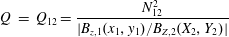 $$\begin{eqnarray}\displaystyle Q & = & \displaystyle Q_{12}=\frac{N_{12}^{2}}{|B_{z,1}(x_{1},y_{1})/B_{Z,2}(X_{2},Y_{2})|}\end{eqnarray}$$
 $$\begin{eqnarray}\displaystyle & = & \displaystyle Q_{21}=\frac{N_{21}^{2}}{|B_{z,2}(x_{2},y_{2})/B_{Z,1}(X_{1},Y_{1})|}.\end{eqnarray}$$
Then, QSLs represent the regions with the highest squashing factor $Q$
. Recently, a computational method to obtain the squashing degree within a 3-D domain was proposed by Pariat & Démoulin (Reference Pariat and Démoulin2012) (see figure 4
c). This was further developed in Tassev & Savcheva (Reference Tassev and Savcheva2016).
$Q$
. Recently, a computational method to obtain the squashing degree within a 3-D domain was proposed by Pariat & Démoulin (Reference Pariat and Démoulin2012) (see figure 4
c). This was further developed in Tassev & Savcheva (Reference Tassev and Savcheva2016).
Since the QSLs form a thin volume (e.g. figure 4 e), one can define the region where the field lines diverge the most in the central part of this volume. In figure 4(f), a transverse cut in the volume is shown, which displays 4 branches marking the characteristic shape of QSLs. This particular region was coined a hyperbolic flux tube (HFT, see Titov et al. Reference Titov, Hornig and Démoulin2002). HFTs can also be understood as the ‘intersection’ of two QSLs, and as such, are generalising the concept of a separator line in three dimensions in the context of QSLs (i.e. since a separator is formed by the intersection of two separatrices). Their shape is particularly reminiscent of an X-point in the transverse cut. At the bottom of figure 4(f) a schema indicates its shapes following the location of the cut in the volume (i.e. those shapes are obtained by doing different cuts of the HFT orthogonal to the local magnetic field). Closer to the anchoring surface, the HFT resembles a line: they are the inner regions within the pale blue and pale magenta traces shown in figure 4(b). Further away from the photosphere, the HFT displays an X-shaped structure. Recently, the concept of the squashing factor to define QSLs and HFTs has been extended to ‘slip-squashing’ factors (Titov et al. Reference Titov, Forbes, Priest, Mikić and Linker2009) (from the discussion in Hesse, Forbes & Birn (Reference Hesse, Forbes and Birn2005)), which allows the characterisation of the change in the magnetic field connections.
2.3 QSLs in the presence of flux ropes: from theory to observations
In the presence of a twisted magnetic field, the quasi-separatrix layers trace the frontier between the twisted magnetic field and the more potential surrounding field (see figure 5). Their traces on the lower boundary show a typical $J$
-shape, with a straight part associated with low-lying coronal loops while the hook region of the
$J$
-shape, with a straight part associated with low-lying coronal loops while the hook region of the $J$
shape is associated with the anchoring region of the flux rope. In Démoulin et al. (Reference Démoulin, Priest and Lonie1996b
), the authors investigated the morphology of the QSLs and especially the hook region: because the QSLs form a thin volume, that delimitates the frontier between differently connected field lines, this volume is also connected to the photospheric surface. Then, the more the magnetic field is twisted, the more complex the QSL photospheric footprint becomes: the QSL swirls around the flux rope as the twist of the structure increases (figure 5
b). QSLs in the presence of flux ropes were also investigated in laboratory experiments. Gekelman, Lawrence & Van Compernolle (Reference Gekelman, Lawrence and Van Compernolle2012) provided experimental evidence that QSLs indeed form in the presence of flux ropes created in a laboratory device.
$J$
shape is associated with the anchoring region of the flux rope. In Démoulin et al. (Reference Démoulin, Priest and Lonie1996b
), the authors investigated the morphology of the QSLs and especially the hook region: because the QSLs form a thin volume, that delimitates the frontier between differently connected field lines, this volume is also connected to the photospheric surface. Then, the more the magnetic field is twisted, the more complex the QSL photospheric footprint becomes: the QSL swirls around the flux rope as the twist of the structure increases (figure 5
b). QSLs in the presence of flux ropes were also investigated in laboratory experiments. Gekelman, Lawrence & Van Compernolle (Reference Gekelman, Lawrence and Van Compernolle2012) provided experimental evidence that QSLs indeed form in the presence of flux ropes created in a laboratory device.

Figure 5. Projected view of a configuration containing a flux rope, as indicated with the dashed-dotted (three turns) and solid (one turn) twisted field lines. The small, dotted field line represent a coronal loop lying underneath the flux rope. The gradient of connectivity between these field lines is indicated with the elongated, bold lines at the photospheric level (QSL trace). Their straight part is associated with the low-lying coronal loop, while the round region is associated with the anchoring region of the twisted field lines. A zoom in the region shows a hook shape of the flux-rope anchoring region, where a higher twist corresponds to a higher number of swirls (adapted from Démoulin et al. (Reference Démoulin, Priest and Lonie1996b )).

Figure 6. (a) Top view of a quadrupolar magnetic configuration (with two bipoles, where the positive (respectively negative) polarity is indicated in magenta (respectively blue)). A photospheric velocity field is applied as a boundary condition so as to reproduce a twisting motion in the small positive polarity. The photospheric traces of the associated QSLs are shown in (b): the highest values of the squashing degree $Q$
are shown in black. The electric currents are shown in greyscale in (c), with the most intense currents shown in white. (d) Side view of the configuration, with (e) showing a transverse cut in the middle of the domain of the coronal current density. The strongest currents are seen to appear at the locations with the highest squashing degree or HFT, as is also shown in the colour-coded zooms of the QSLs (f) and the currents (g) (adapted from Aulanier et al. (Reference Aulanier, Pariat and Démoulin2005)).
$Q$
are shown in black. The electric currents are shown in greyscale in (c), with the most intense currents shown in white. (d) Side view of the configuration, with (e) showing a transverse cut in the middle of the domain of the coronal current density. The strongest currents are seen to appear at the locations with the highest squashing degree or HFT, as is also shown in the colour-coded zooms of the QSLs (f) and the currents (g) (adapted from Aulanier et al. (Reference Aulanier, Pariat and Démoulin2005)).
Because of the strong distortion of the magnetic field line mapping at QSLs, the latter were proposed as preferential locations for current buildup (Démoulin et al. Reference Démoulin, Hénoux, Priest and Mandrini1996a ; Démoulin Reference Démoulin, Innes, Lagg and Solanki2005). This was investigated in numerical simulations, and several authors indeed showed the generic formation of strong current density regions at QSLs, as indicated in figure 6 (Aulanier et al. Reference Aulanier, Pariat and Démoulin2005; Pariat, Aulanier & Démoulin Reference Pariat, Aulanier, Démoulin, Barret, Casoli, Lagache, Lecavelier and Pagani2006; Masson et al. Reference Masson, Pariat, Aulanier and Schrijver2009; Effenberger et al. Reference Effenberger, Thust, Arnold, Grauer and Dreher2011; Craig & Effenberger Reference Craig and Effenberger2014). However, an exact one-to-one correspondence between the localisation of the highest squashing degree values (HFT) and the highest current densities is not necessarily found, as was shown in Wilmot-Smith, Hornig & Pontin (Reference Wilmot-Smith, Hornig and Pontin2009) and (Janvier et al. Reference Janvier, Aulanier, Pariat and Démoulin2013). The correspondence of QSLs with regions of reconnection is not limited to MHD models generally investigated in the context of the Sun. Recent kinetic simulations in three dimensions such as by Wendel et al. (Reference Wendel, Olson, Hesse, Aunai, Kuznetsova, Karimabadi, Daughton and Adrian2013) have shown that QSLs are associated with areas of large gradients of parallel electric field, which provide a new understanding on the determination of reconnection sites in predominantly collisionless plasmas such as the Earth’s magnetosphere. Since electric currents are extremely difficult to directly investigate in the solar corona (because of the absence of reliable direct observations of magnetic fields in the Sun’s atmosphere), simulations provide a useful environment to understand the formation and the evolution of currents in the presence of QSLs, such as shown in figure 6. Recently, proxies of coronal currents, such as their photospheric signatures, have been used to investigate the similarities in the location, morphology and evolution of QSLs and currents. They show the correspondence expected from numerical simulations, as detailed in § 3.4.
Since QSLs generalise the concept of separatrices and are associated with locations of electric currents, and hence reconnection, investigation of the topology of flaring magnetic field configurations naturally led to the search for QSLs and their relation with flares. For example, Démoulin et al. (Reference Démoulin, Hénoux, Priest and Mandrini1996a
, Reference Démoulin, Bagala, Mandrini, Hénoux and Rovira1997) used modelling techniques of the coronal field to reproduce magnetograms of flaring regions and computed QSL locations. In these works, the authors found that locations where H $\unicode[STIX]{x1D6FC}$
brightening was observed were related to locations of QSLs. Furthermore, QSLs can also be found in the presence of a null point: such a configuration was also investigated in a circular ribbon flare, using data-driven simulations (Masson et al.
Reference Masson, Pariat, Aulanier and Schrijver2009). Since then, investigating the locations of QSLs has proved to be successful at interpreting a large variety of flaring regions (e.g. Schmieder et al.
Reference Schmieder, Aulanier, Demoulin, van Driel-Gesztelyi, Roudier, Nitta and Cauzzi1997; Bagalá et al.
Reference Bagalá, Mandrini, Rovira and Démoulin2000; Mandrini et al.
Reference Mandrini, Demoulin, Schmieder, Deluca, Pariat and Uddin2006; Restante, Aulanier & Parnell Reference Restante, Aulanier and Parnell2009; Chandra et al.
Reference Chandra, Schmieder, Mandrini, Démoulin, Pariat, Török and Uddin2011).
$\unicode[STIX]{x1D6FC}$
brightening was observed were related to locations of QSLs. Furthermore, QSLs can also be found in the presence of a null point: such a configuration was also investigated in a circular ribbon flare, using data-driven simulations (Masson et al.
Reference Masson, Pariat, Aulanier and Schrijver2009). Since then, investigating the locations of QSLs has proved to be successful at interpreting a large variety of flaring regions (e.g. Schmieder et al.
Reference Schmieder, Aulanier, Demoulin, van Driel-Gesztelyi, Roudier, Nitta and Cauzzi1997; Bagalá et al.
Reference Bagalá, Mandrini, Rovira and Démoulin2000; Mandrini et al.
Reference Mandrini, Demoulin, Schmieder, Deluca, Pariat and Uddin2006; Restante, Aulanier & Parnell Reference Restante, Aulanier and Parnell2009; Chandra et al.
Reference Chandra, Schmieder, Mandrini, Démoulin, Pariat, Török and Uddin2011).
From then on, the locations and the morphology of sudden flare brightenings were compared with the locations of QSLs found with a magnetic field model. Over the years, the techniques were refined, helped by higher spatial resolution instruments as well as more refined modelling techniques (such as magnetic field extrapolations). To give an example, the ribbons of eruptive flares were often compared with QSLs found in the presence of flux ropes: indeed, this type of flare often displays the presence of two flare ribbons appearing in H $\unicode[STIX]{x1D6FC}$
(Chandra et al.
Reference Chandra, Schmieder, Aulanier and Malherbe2009), and in particular these ribbons often display a
$\unicode[STIX]{x1D6FC}$
(Chandra et al.
Reference Chandra, Schmieder, Aulanier and Malherbe2009), and in particular these ribbons often display a $\unicode[STIX]{x1D611}$
-shaped structure. This morphology is very similar to the analytical shapes found for QSLs in the presence of twisted flux tubes (see above and figure 5), as well as in recent 3-D MHD numerical simulations of eruptive flares (see figure 3 in Janvier et al. (Reference Janvier, Aulanier, Pariat and Démoulin2013)).
$\unicode[STIX]{x1D611}$
-shaped structure. This morphology is very similar to the analytical shapes found for QSLs in the presence of twisted flux tubes (see above and figure 5), as well as in recent 3-D MHD numerical simulations of eruptive flares (see figure 3 in Janvier et al. (Reference Janvier, Aulanier, Pariat and Démoulin2013)).

Figure 7. (a) Sigmoidal region seen by the XRT instrument aboard Hinode from which a magnetic model is constructed, shown with a sample of field lines in (b). Panels (c,e,g) show the numerical simulation of an unstable flux rope, while (d,f,h) show similar plots for a magnetic configuration derived from observations (b). The (near) photospheric traces of the QSLs for a numerical flux-rope simplified model are shown in (c). They are compared in (d) with that of the configuration created by a flux rope inserted in the extrapolated potential magnetic field of the magnetogram shown in (b). They both display the typical $\unicode[STIX]{x1D611}$
shape expected in the presence of a flux rope. A transverse cut (dashed black lines in c and d) is shown in the magnetic field numerical model (e) and the extrapolated magnetic field (f), where the location of the highest values of the squashing degree
$\unicode[STIX]{x1D611}$
shape expected in the presence of a flux rope. A transverse cut (dashed black lines in c and d) is shown in the magnetic field numerical model (e) and the extrapolated magnetic field (f), where the location of the highest values of the squashing degree $Q$
is found underneath the flux rope in both cases. A zoom indicate the presence of a HFT in (g,h) (adapted from Savcheva et al. (Reference Savcheva, Pariat, van Ballegooijen, Aulanier and DeLuca2012a
)).
$Q$
is found underneath the flux rope in both cases. A zoom indicate the presence of a HFT in (g,h) (adapted from Savcheva et al. (Reference Savcheva, Pariat, van Ballegooijen, Aulanier and DeLuca2012a
)).
Savcheva et al. (Reference Savcheva, Pariat, van Ballegooijen, Aulanier and DeLuca2012a
) investigated the shape of QSLs for a magnetic field model of an active region which was associated with the presence of a sigmoid (a region where the coronal loops display $J$
- or
$J$
- or $S$
-shaped features, indicative of a flux rope, see e.g. Green et al.
Reference Green, Kliem, Török, van Driel-Gesztelyi and Attrill2007; McKenzie & Canfield Reference McKenzie and Canfield2008). They model the flux rope associated with the sigmoidal region using the flux-rope insertion method (see van Ballegooijen Reference van Ballegooijen2004). With a magnetic model of the active region, the authors could investigate the connectivity change in the volume of interest, and look in more details at the morphology of the QSLs. Some of these results are reproduced in figure 7, where it shows that the photospheric traces of the QSLs are much more complex than in analytical and simulation models, yet still displaying a hooked,
$S$
-shaped features, indicative of a flux rope, see e.g. Green et al.
Reference Green, Kliem, Török, van Driel-Gesztelyi and Attrill2007; McKenzie & Canfield Reference McKenzie and Canfield2008). They model the flux rope associated with the sigmoidal region using the flux-rope insertion method (see van Ballegooijen Reference van Ballegooijen2004). With a magnetic model of the active region, the authors could investigate the connectivity change in the volume of interest, and look in more details at the morphology of the QSLs. Some of these results are reproduced in figure 7, where it shows that the photospheric traces of the QSLs are much more complex than in analytical and simulation models, yet still displaying a hooked, $\unicode[STIX]{x1D611}$
shape. A transverse cut in the middle of the twisted structure also shows the presence of an
$\unicode[STIX]{x1D611}$
shape. A transverse cut in the middle of the twisted structure also shows the presence of an $X$
-shaped region that is reminiscent of the HFT (figure 7
e–h). Such a work therefore provides observational evidence that HFTs and associated QSLs are generic features found in the presence of sigmoidal regions and flux ropes.
$X$
-shaped region that is reminiscent of the HFT (figure 7
e–h). Such a work therefore provides observational evidence that HFTs and associated QSLs are generic features found in the presence of sigmoidal regions and flux ropes.
Recently, such an analysis has been extended to a variety of flaring regions and with different techniques. For example, Zhao et al. (Reference Zhao, Gilchrist, Aulanier, Schmieder, Pariat and Li2016) studied a flaring region and applied another technique to reconstruct the magnetic field of the region, namely, a nonlinear force-free field model (following the technique of Gilchrist & Wheatland Reference Gilchrist and Wheatland2013). They found similar morphologies in the shape of the QSLs as in Savcheva et al. (Reference Savcheva, Pariat, van Ballegooijen, Aulanier and DeLuca2012a ). As such, the morphology of QSLs in the presence of erupting flux ropes is independent of the extrapolation method. This is expected because of the structural stability of QSLs, in contrast to the presence and the location of null points and associated separatrices, (see Démoulin et al. Reference Démoulin, Hénoux and Mandrini1994a ; Janvier et al. Reference Janvier, Savcheva, Pariat, Tassev, Millholland, Bommier, McCauley, McKillop and Dougan2016, on the influence of the extrapolations on the stability of null points and QSLs). Furthermore, the shapes of the QSLs can be directly compared with that of the flare ribbons.
Then, evolving the magnetic model of an active region, for example by an MHD evolution or a magnetofrictional relaxation (in the case of an unstable flux rope), also allows the investigation of the evolution of QSLs. The multiple time sequences of these evolutions can provide snapshots that can be compared with observations of flare ribbons, as presented in Savcheva et al. (Reference Savcheva, Pariat, McKillop, McCauley, Hanson, Su, Werner and Deluca2015, Reference Savcheva, Pariat, McKillop, McCauley, Hanson, Su and Deluca2016), Janvier et al. (Reference Janvier, Savcheva, Pariat, Tassev, Millholland, Bommier, McCauley, McKillop and Dougan2016).
As such, the search for QSLs in a magnetic field reveals the coronal locations of the dissipation, as well as a tool to interpret the photospheric signatures of reconnection as seen with flare ribbons.
3 Dissipation layer
3.1 Dissipation process
The first developments in the theory of magnetic field reconnection were accompanied by a description of the dissipation process taking place in current layers. The diffusion terms appear in Ohm’s law as non-ideal terms. In its simplest description (resistive MHD for a single fluid), the non-ideal departure is described with $\unicode[STIX]{x1D702}\boldsymbol{J}$
:
$\unicode[STIX]{x1D702}\boldsymbol{J}$
:
 $$\begin{eqnarray}\boldsymbol{E}+\boldsymbol{v}\times \boldsymbol{B}=\unicode[STIX]{x1D702}\boldsymbol{J},\end{eqnarray}$$
where $\unicode[STIX]{x1D702}$
is the plasma resistivity (a measure of the collisionality of the plasma, see Spitzer (Reference Spitzer1956)) and
$\unicode[STIX]{x1D702}$
is the plasma resistivity (a measure of the collisionality of the plasma, see Spitzer (Reference Spitzer1956)) and $\boldsymbol{J}$
is the electric current density vector. The effect of finite conductivity on the diffusion of magnetic fields was already investigated for several configurations by Parker & Krook (Reference Parker and Krook1956). However, simply considering the diffusion of magnetic fields in the corona provides time scales (years) that are considerably larger than that of flares (minutes). Then, Petschek (Reference Petschek1964) introduced another reconnection model where he instead considered a much shorter current sheet, which provided the much greater inflow speed needed for fast reconnection. In his model, he overcame the elongation of the current layers (from an X shape to a double Y shape) by invoking the appearance of oblique, magnetohydrodynamic, standing shock waves which develop at the edges of the current layer. Then, the reconnection rate is enhanced by hydromagnetic actions (since the waves allow magnetic energy conversion) outside the diffusion region, while the ohmic dissipation only occurs in the very small current layer. However, its mechanism was doubted (Green & Sweet Reference Green and Sweet1967) and later proved to not be reproducible in numerical simulations either (Biskamp Reference Biskamp1986), unless when some variation in the resistivity was accounted for (see Baty, Forbes & Priest Reference Baty, Forbes and Priest2009). Further developments of the Sweet–Parker and Petschek models were compared, such as by Kulsrud (Reference Kulsrud2001), who investigated analytically the similarities between the Sweet–Parker and the Petschek models. Both are found to have a similar reconnection rate in case of constant resistivity due to the imposed condition that the length of Petschek’s diffusive layer is not a free parameter, a condition that was not taken into account in the original work. The Sweet–Parker current sheet, which describes a stationary model, is quite restrictive compared with the possible evolutions of current sheets, as described below in § 3.2. We also refer the reader to the historical evolution and recent advances deriving from the Sweet–Parker configuration discussed in Loureiro & Uzdensky (Reference Loureiro and Uzdensky2016).
$\boldsymbol{J}$
is the electric current density vector. The effect of finite conductivity on the diffusion of magnetic fields was already investigated for several configurations by Parker & Krook (Reference Parker and Krook1956). However, simply considering the diffusion of magnetic fields in the corona provides time scales (years) that are considerably larger than that of flares (minutes). Then, Petschek (Reference Petschek1964) introduced another reconnection model where he instead considered a much shorter current sheet, which provided the much greater inflow speed needed for fast reconnection. In his model, he overcame the elongation of the current layers (from an X shape to a double Y shape) by invoking the appearance of oblique, magnetohydrodynamic, standing shock waves which develop at the edges of the current layer. Then, the reconnection rate is enhanced by hydromagnetic actions (since the waves allow magnetic energy conversion) outside the diffusion region, while the ohmic dissipation only occurs in the very small current layer. However, its mechanism was doubted (Green & Sweet Reference Green and Sweet1967) and later proved to not be reproducible in numerical simulations either (Biskamp Reference Biskamp1986), unless when some variation in the resistivity was accounted for (see Baty, Forbes & Priest Reference Baty, Forbes and Priest2009). Further developments of the Sweet–Parker and Petschek models were compared, such as by Kulsrud (Reference Kulsrud2001), who investigated analytically the similarities between the Sweet–Parker and the Petschek models. Both are found to have a similar reconnection rate in case of constant resistivity due to the imposed condition that the length of Petschek’s diffusive layer is not a free parameter, a condition that was not taken into account in the original work. The Sweet–Parker current sheet, which describes a stationary model, is quite restrictive compared with the possible evolutions of current sheets, as described below in § 3.2. We also refer the reader to the historical evolution and recent advances deriving from the Sweet–Parker configuration discussed in Loureiro & Uzdensky (Reference Loureiro and Uzdensky2016).
A more complete description of the physical dissipation mechanism in current layers can include ambipolar diffusion, which is effective in partially ionised gases of sufficient density (Piddington Reference Piddington1954b ). This process is related to the drift of the plasma with respect to the neutrals in the presence of a magnetic field (see Zweibel Reference Zweibel, Lazarian, de Gouveia Dal Pino and Melioli2015, for more insights on the phenomenon and its importance in astrophysical systems). The ambipolar diffusion does not itself lead to magnetic reconnection, but as it squeezes the magnetic field lines together, they end up ‘piling up’, permitting a more efficient dissipation (see also Parker Reference Parker1963). Ambipolar diffusion has recently been revisited in the context of reconnection in the chromosphere, where the plasma is dense (see e.g. Leake, Lukin & Linton Reference Leake, Lukin and Linton2013). However, it is dubious that ambipolar diffusion may have a strong role in the corona since the density there is rather low and the corona is fully ionised.
The effects of turbulence on reducing the plasma conductivity were already pointed out by Sweet (Reference Sweet1950). Wentzel (Reference Wentzel1963) proposed also early on that the increased dissipation due to turbulence can increase the magnetic annihilation rate. Plasma experiments such as those conducted by Baum & Bratenahl (Reference Baum and Bratenahl1976) then showed direct observations of rapid magnetic field reconnection, and transition from slow to fast reconnection due to an anomalous resistivity, validating such reconnection models. The effect of anomalous resistivity was studied numerically in different current sheet configurations: it was for example shown to account for the transition from a Sweet–Parker-like current layer to a Petscheck-type current layer (Baty et al. Reference Baty, Forbes and Priest2009; Baty, Forbes & Priest Reference Baty, Forbes and Priest2014). The effects of stochastic magnetic fields were also shown to increase the reconnection rate (e.g. Lazarian & Vishniac Reference Lazarian and Vishniac1999).
A large body of work has investigated the reconnection mechanism at small scales. Effects such as the Hall term (Piddington Reference Piddington1954a ), the ion inertia term and the electron pressure density can play a role in the reconnection mechanism and can change the energy partition. The relevant Ohm’s law in such a case is as follows:
 $$\begin{eqnarray}\boldsymbol{E}+\boldsymbol{v}\times \boldsymbol{B}=\unicode[STIX]{x1D702}\boldsymbol{J}+\frac{1}{en}\boldsymbol{J}\times \boldsymbol{B}-\frac{1}{en}\unicode[STIX]{x1D735}\boldsymbol{\cdot }\boldsymbol{P}_{e}-\frac{m_{e}}{e}\frac{\text{d}\boldsymbol{v}e}{\text{d}t},\end{eqnarray}$$
where the first term (on the right-hand side of the equation) is the plasma resistivity term, the second the Hall term, the third the electron pressure tensor and the remaining term represents the electron inertia.
These last three terms arise where the traditional MHD formalism breaks down for a current sheet that is thin enough, i.e. the diffusion region becomes thinner than the ion skin depth (in such a case, we generally refer to reconnection as being collisionless). Note that adding more terms to Ohm’s law means that the physics related to the ions and the electrons is more complete than a description where the plasma is considered as a single species fluid, as can be seen by comparing (3.1) and (3.2). For example, the Hall term arises when magnetic drifts are considered: this relates to the motion separation between electrons and ions, i.e. electric currents, which then need to be added as a correction to Ohm’s law (the $(ne)^{-1}\boldsymbol{J}\times \boldsymbol{B}$
term, see numerical developments in Huba Reference Huba2003). We note that a careful interpretation of the Hall term is needed, since the term itself is not a magnetic field connectivity breaking term. Indeed, the Hall term decouples the ions and the electrons, and the magnetic field remains tied to the electrons (meaning that at the electron scale, the magnetic field still remains ‘frozen-in’). The importance of small-scale effects was pointed out by Birn et al. (Reference Birn, Drake, Shay, Rogers, Denton, Hesse, Kuznetsova, Ma, Bhattacharjee and Otto2001), where the authors investigated the effects of different numerical set-ups with different expressions of the Ohm’s law. In particular, any implementation (MHD or particle-in-cell (PIC)) containing the Hall term gave similar results, contrary to the simple resistive MHD description (see figure 8
a). The decoupling of the ions and the electrons are shown in figure 8(b), where the diffusion region is defined differently (with different physical effects) for the ions and the electrons. Studies of small-scale effects therefore include Hall fields (Drake, Shay & Swisdak Reference Drake, Shay and Swisdak2008), anisotropic pressure (Birn & Hesse Reference Birn and Hesse2001), electron dynamics and viscosity (Ma & Bhattacharjee Reference Ma and Bhattacharjee1996; Hesse, Kuznetsova & Birn Reference Hesse, Kuznetsova and Birn2004; Cai & Li Reference Cai and Li2008), while reviews of these effects can also be found in Porcelli et al. (Reference Porcelli, Borgogno, Califano, Grasso, Ottaviani and Pegoraro2002), Shay et al. (Reference Shay, Drake, Swisdak and Rogers2004), Büchner (Reference Büchner2007).
$(ne)^{-1}\boldsymbol{J}\times \boldsymbol{B}$
term, see numerical developments in Huba Reference Huba2003). We note that a careful interpretation of the Hall term is needed, since the term itself is not a magnetic field connectivity breaking term. Indeed, the Hall term decouples the ions and the electrons, and the magnetic field remains tied to the electrons (meaning that at the electron scale, the magnetic field still remains ‘frozen-in’). The importance of small-scale effects was pointed out by Birn et al. (Reference Birn, Drake, Shay, Rogers, Denton, Hesse, Kuznetsova, Ma, Bhattacharjee and Otto2001), where the authors investigated the effects of different numerical set-ups with different expressions of the Ohm’s law. In particular, any implementation (MHD or particle-in-cell (PIC)) containing the Hall term gave similar results, contrary to the simple resistive MHD description (see figure 8
a). The decoupling of the ions and the electrons are shown in figure 8(b), where the diffusion region is defined differently (with different physical effects) for the ions and the electrons. Studies of small-scale effects therefore include Hall fields (Drake, Shay & Swisdak Reference Drake, Shay and Swisdak2008), anisotropic pressure (Birn & Hesse Reference Birn and Hesse2001), electron dynamics and viscosity (Ma & Bhattacharjee Reference Ma and Bhattacharjee1996; Hesse, Kuznetsova & Birn Reference Hesse, Kuznetsova and Birn2004; Cai & Li Reference Cai and Li2008), while reviews of these effects can also be found in Porcelli et al. (Reference Porcelli, Borgogno, Califano, Grasso, Ottaviani and Pegoraro2002), Shay et al. (Reference Shay, Drake, Swisdak and Rogers2004), Büchner (Reference Büchner2007).

Figure 8. Comparison of resistive MHD and kinetic descriptions of the current layer. (a) Results of the Geospace Environmental Modeling (GEM) magnetic reconnection challenge, where several codes (MHD and PIC) were tested to investigate the effects of the nonlinear terms described in the generalised Ohm’s law. It was found that codes that include the Hall term did not differ much one from another, while a conventional resistive MHD description of reconnection did not agree with all the other results. Here, the time evolution of the reconnected flux in those simulations are shown to indicate the differences (adapted from Birn et al. (Reference Birn, Drake, Shay, Rogers, Denton, Hesse, Kuznetsova, Ma, Bhattacharjee and Otto2001)). (b) Description of the magnetic field geometry in collisionless reconnection, where the flows of the ions and the electrons are decoupled in the diffusion area (adapted from Zweibel & Yamada (Reference Zweibel and Yamada2009)).
3.2 Current layer formation and evolution
In the Sweet and Parker mechanism (Sweet Reference Sweet1956; Parker Reference Parker1957b ; Sweet Reference Sweet and Lehnert1958a ), and as well as in the Petschek mechanism (Petschek Reference Petschek1964), reconnection is considered analytically in a steady-state current layer, treated as a boundary layer where the plasma outside of this region is considered as current free and perfectly conducting. Such models are useful in obtaining the magnetic energy conversion (or reconnection) rates (Parker Reference Parker1963), as well as providing the geometrical characteristics of the current layer (Priest & Raadu Reference Priest and Raadu1975; Tur & Priest Reference Tur and Priest1976). However, in the works of Green & Sweet (Reference Green and Sweet1967) and Petschek & Thorne (Reference Petschek and Thorne1967), the authors had to modify the original Petschek reconnection scenario (e.g. with additional waves) as they recognised that the region where ohmic diffusion takes place at the intersection of two shocks is too thin to be hydrodynamic. Friedman & Hamberger (Reference Friedman and Hamberger1968) also pointed out that the current density in Petschek’s original model violates the two-stream instability criterion. Finally, Syrovatskii’s work (Syrovatskii Reference Syrovatskii1966) on dynamic dissipation in current layers throws some doubt on whether a quasi-steady state can be achieved at all.
It is necessary to remind the reader that reconnection in such steady-state configurations is driven by boundary motions: the magnetic field is forced to move into the dissipation layer by a driving inflow around the reconnecting region (Hahm & Kulsrud Reference Hahm and Kulsrud1985; Wang, Ma & Bhattacharjee Reference Wang, Ma and Bhattacharjee1996). The rate of reconnection or energy conversion is therefore dictated by the inflow of magnetic flux brought to the dissipation region. The dynamics of the coronal field can infer flows which velocity fields drive/enhance the reconnection in the current layer. Therefore, a Sweet–Parker regime is often a misnomer when describing reconnection processes occurring in the Sun’s corona, since the inflows from the surroundings of the reconnection region are not themselves steady state. How the reconnection rate is actually determined by boundary conditions is still poorly understood (see the discussions in Comisso & Bhattacharjee Reference Comisso and Bhattacharjee2016). Recently, Forbes et al. (Reference Forbes, Priest, Seaton and Litvinenko2013), Baty et al. (Reference Baty, Forbes and Priest2014) have argued that the rate of reconnection is more likely to be controlled by the non-uniformity of the normal magnetic field in reconnecting layers rather than by the boundary conditions.
Steady-state, driven reconnection models lose the description needed to explain the onset of flares. Indeed, as was already recognised by Gold & Hoyle (Reference Gold and Hoyle1960), it is important for a model to include the suddenness of flaring events. In particular, they acknowledged the necessity of force-free fields to progressively store free magnetic energy, which exist prior to the flare. They also recognised the need to have a storage mechanism and release mechanism, invoking the existence of instabilities.
The instability of current layers gained some attention in the early stages of plasma laboratory experiments, especially because they were found to be detrimental to the realisation of fusion, the process to harness a star-like energy. Then, Furth, Killeen & Rosenbluth (Reference Furth, Killeen and Rosenbluth1963) proposed that a resistive instability takes place in the current layer, which leads to a readjustment of the magnetic field in a configuration of lower energy. This lower state is characterised by the presence of magnetic islands (2-D transverse cuts of 3-D twisted flux ropes, appearing as nested magnetic field lines). As it gives a shredded structure to the current layer, this instability was coined the tearing instability. Furthermore, the interest in this mechanism for solar flare application lies in the fact that the time scale of the tearing instability was much smaller than a simple resistive diffusion of the equilibrium (although the instability grows more slowly than MHD instabilities, as $t_{A}<t_{T}<t_{R}$
where
$t_{A}<t_{T}<t_{R}$
where $t_{A}$
is the MHD time scale (Alfvén time),
$t_{A}$
is the MHD time scale (Alfvén time), $t_{T}$
the tearing instability time scale and
$t_{T}$
the tearing instability time scale and $t_{R}$
the resistive diffusion time scaling with
$t_{R}$
the resistive diffusion time scaling with $\unicode[STIX]{x1D702}^{-1}$
). Putting numbers for the solar corona, Jaggi (Reference Jaggi1963), Sturrock (Reference Sturrock and Kiepenheuer1968), Kliem (Reference Kliem1995) found that the e-folding time of the instability was small enough to account for the time scale generally associated with solar flares (although this is only valid in the case of extremely small scales, see discussions in Del Zanna et al.
Reference Del Zanna, Landi, Papini, Pucci and Velli2016), while Spicer (Reference Spicer1981) put forward this instability as a possible mechanism for particle acceleration. These findings were nonetheless challenged by the incapacity of a single tearing layer to provide the necessary current dissipation to account for the thermal emissions seen in flares (e.g. La Rosa Reference La Rosa1990). A more complex system of small-scale current layers (or multiple tearing layers) was proposed instead. Simulations in 2.5 dimensions (i.e. with an invariant direction) of current sheets in the context of solar flares were also recently investigated (Shibata & Tanuma Reference Shibata and Tanuma2001; Lynch et al.
Reference Lynch, Edmondson, Kazachenko and Guidoni2016), where the breaking up of the current layer in multiple plasmoids was shown. The connection between plasmoids investigated in numerical simulations, whether two- or three-dimensional, and observations of solar flares, are discussed in more details in § 4.3.
$\unicode[STIX]{x1D702}^{-1}$
). Putting numbers for the solar corona, Jaggi (Reference Jaggi1963), Sturrock (Reference Sturrock and Kiepenheuer1968), Kliem (Reference Kliem1995) found that the e-folding time of the instability was small enough to account for the time scale generally associated with solar flares (although this is only valid in the case of extremely small scales, see discussions in Del Zanna et al.
Reference Del Zanna, Landi, Papini, Pucci and Velli2016), while Spicer (Reference Spicer1981) put forward this instability as a possible mechanism for particle acceleration. These findings were nonetheless challenged by the incapacity of a single tearing layer to provide the necessary current dissipation to account for the thermal emissions seen in flares (e.g. La Rosa Reference La Rosa1990). A more complex system of small-scale current layers (or multiple tearing layers) was proposed instead. Simulations in 2.5 dimensions (i.e. with an invariant direction) of current sheets in the context of solar flares were also recently investigated (Shibata & Tanuma Reference Shibata and Tanuma2001; Lynch et al.
Reference Lynch, Edmondson, Kazachenko and Guidoni2016), where the breaking up of the current layer in multiple plasmoids was shown. The connection between plasmoids investigated in numerical simulations, whether two- or three-dimensional, and observations of solar flares, are discussed in more details in § 4.3.
A variety of resistive instabilities have since then been studied, such as the resistive kink (with mode number $m=1$
, also coined fast tearing as its growth rate scales with
$m=1$
, also coined fast tearing as its growth rate scales with $\unicode[STIX]{x1D702}^{1/3}$
, see e.g. Rosenbluth, Dagazian & Rutherford Reference Rosenbluth, Dagazian and Rutherford1973; Hazeltine, Meiss & Morrison Reference Hazeltine, Meiss and Morrison1986; Waelbroeck Reference Waelbroeck1989; Watanabe, Sato & Nakayama Reference Watanabe, Sato and Nakayama1995). Although the resistive kink instability has been extensively studied in the context of tokamak plasmas, kink modes (resistive in nature) can be put forward to explain the onset and subsequent magnetic energy dissipation of eruptive flares. This was discussed in Hood & Priest (Reference Hood and Priest1979) for line-tied field lines (relevant in the context of solar flares), and numerical simulations of kink unstable flux ropes were compared with observations in Török & Kliem (Reference Török and Kliem2005). Furthermore, multiple tearing instabilities can greatly enhance the reconnection rate in the nonlinear regime due to coupling between islands (where the reconnection outflow of a magnetic island can increase the inflow of a nearby reconnection site, e.g. Pritchett, Lee & Drake Reference Pritchett, Lee and Drake1980; Ishii, Azumi & Kishimoto Reference Ishii, Azumi and Kishimoto2002; Bierwage et al.
Reference Bierwage, Hamaguchi, Wakatani, Benkadda and Leoncini2005; Wang et al.
Reference Wang, Wang, Dong, Lei, Long, Mou and Qu2007; Janvier, Kishimoto & Li Reference Janvier, Kishimoto and Li2011; Wang, Yokoyama & Isobe Reference Wang, Yokoyama and Isobe2015). Finally the effect of line-tying, relevant in the context of coronal magnetic field, was investigated in Delzanno & Finn (Reference Delzanno and Finn2008), which found that the growth rate scaled with
$\unicode[STIX]{x1D702}^{1/3}$
, see e.g. Rosenbluth, Dagazian & Rutherford Reference Rosenbluth, Dagazian and Rutherford1973; Hazeltine, Meiss & Morrison Reference Hazeltine, Meiss and Morrison1986; Waelbroeck Reference Waelbroeck1989; Watanabe, Sato & Nakayama Reference Watanabe, Sato and Nakayama1995). Although the resistive kink instability has been extensively studied in the context of tokamak plasmas, kink modes (resistive in nature) can be put forward to explain the onset and subsequent magnetic energy dissipation of eruptive flares. This was discussed in Hood & Priest (Reference Hood and Priest1979) for line-tied field lines (relevant in the context of solar flares), and numerical simulations of kink unstable flux ropes were compared with observations in Török & Kliem (Reference Török and Kliem2005). Furthermore, multiple tearing instabilities can greatly enhance the reconnection rate in the nonlinear regime due to coupling between islands (where the reconnection outflow of a magnetic island can increase the inflow of a nearby reconnection site, e.g. Pritchett, Lee & Drake Reference Pritchett, Lee and Drake1980; Ishii, Azumi & Kishimoto Reference Ishii, Azumi and Kishimoto2002; Bierwage et al.
Reference Bierwage, Hamaguchi, Wakatani, Benkadda and Leoncini2005; Wang et al.
Reference Wang, Wang, Dong, Lei, Long, Mou and Qu2007; Janvier, Kishimoto & Li Reference Janvier, Kishimoto and Li2011; Wang, Yokoyama & Isobe Reference Wang, Yokoyama and Isobe2015). Finally the effect of line-tying, relevant in the context of coronal magnetic field, was investigated in Delzanno & Finn (Reference Delzanno and Finn2008), which found that the growth rate scaled with $\unicode[STIX]{x1D702}$
for small structure lengths (compared with the system size), while it was tearing-like for long structures. This may be of interest considering different reconnecting coronal loops in the context of say, nanoflares involving small loops versus the larger structures generally seen in flares. It should also be noted that recently, the tearing mode has been revisited in the context of current sheets with large aspect ratios. In such cases, it is possible to find current layers for which the tearing mode growth rate is of order unity and independent of the Reynolds number: such modes are coined ‘ideal tearing modes’ and are interesting to consider in the context of solar flares (Pucci & Velli Reference Pucci and Velli2014; Landi et al.
Reference Landi, Del Zanna, Papini, Pucci and Velli2015; Del Sarto et al.
Reference Del Sarto, Pucci, Tenerani and Velli2016; Del Zanna et al.
Reference Del Zanna, Landi, Papini, Pucci and Velli2016).
$\unicode[STIX]{x1D702}$
for small structure lengths (compared with the system size), while it was tearing-like for long structures. This may be of interest considering different reconnecting coronal loops in the context of say, nanoflares involving small loops versus the larger structures generally seen in flares. It should also be noted that recently, the tearing mode has been revisited in the context of current sheets with large aspect ratios. In such cases, it is possible to find current layers for which the tearing mode growth rate is of order unity and independent of the Reynolds number: such modes are coined ‘ideal tearing modes’ and are interesting to consider in the context of solar flares (Pucci & Velli Reference Pucci and Velli2014; Landi et al.
Reference Landi, Del Zanna, Papini, Pucci and Velli2015; Del Sarto et al.
Reference Del Sarto, Pucci, Tenerani and Velli2016; Del Zanna et al.
Reference Del Zanna, Landi, Papini, Pucci and Velli2016).

Figure 9. Three-dimensional representation and vertical cuts of an erupting flux rope. Results of the numerical simulation of a torus-unstable flux-rope expansion with the OHM code (Aulanier et al.
Reference Aulanier, Janvier and Schmieder2012). (a–c) Field lines showing the expanding magnetic field as time passes by (the times represented here are $t=15t_{A},30t_{A},45t_{A}$
). A 2-D transverse cut (black dashed lines in a–c) of the QSLs is shown, for all three times, in (d–f). The QSLs delimitate different magnetic field domains related to the flux rope, flare loops and surrounding field. The region of the QSLs where the magnetic connectivity changes the most is indicated as the HFT (see § 2.2). A similar cut for the volumic current density
$t=15t_{A},30t_{A},45t_{A}$
). A 2-D transverse cut (black dashed lines in a–c) of the QSLs is shown, for all three times, in (d–f). The QSLs delimitate different magnetic field domains related to the flux rope, flare loops and surrounding field. The region of the QSLs where the magnetic connectivity changes the most is indicated as the HFT (see § 2.2). A similar cut for the volumic current density $J$
is shown in (g–i). The time evolution shows a thinning of the central current layer (indicated with red arrows), with an increased current density. The reconnection region and the top of the reconnected field lines move upward as time passes, as indicated with the yellow and green arrows (adapted from Janvier et al.
Reference Janvier, Aulanier, Pariat and Démoulin2013).
$J$
is shown in (g–i). The time evolution shows a thinning of the central current layer (indicated with red arrows), with an increased current density. The reconnection region and the top of the reconnected field lines move upward as time passes, as indicated with the yellow and green arrows (adapted from Janvier et al.
Reference Janvier, Aulanier, Pariat and Démoulin2013).

Figure 10. Traces on the photospheric boundary of the QSLs and current density for an erupting flux rope. (a) The 3-D volume of the current layer during a flux-rope ejection, as simulated by Kliem et al. (Reference Kliem, Su, van Ballegooijen and DeLuca2013) and similar to the simulation of Aulanier et al. (Reference Aulanier, Janvier and Schmieder2012) and Janvier et al. (Reference Janvier, Aulanier, Pariat and Démoulin2013). (b) A model of a flux rope (solid think line) underneath overlying arcades (dashed lines), showing the hooked, $\unicode[STIX]{x1D611}$
-shaped QSLs (thick lines), as was first investigated in Démoulin et al. (Reference Démoulin, Priest and Lonie1996b
). (c) Top view of the photospheric (
$\unicode[STIX]{x1D611}$
-shaped QSLs (thick lines), as was first investigated in Démoulin et al. (Reference Démoulin, Priest and Lonie1996b
). (c) Top view of the photospheric ( $z=0$
) footprints of the vertical component of the current density vector
$z=0$
) footprints of the vertical component of the current density vector $J_{z}$
in greyscale for the flux-rope eruption simulation of Aulanier et al. (Reference Aulanier, Janvier and Schmieder2012). The magnetic polarities are shown in magenta (positive) and cyan (negative). (d) Same view for the photospheric footprints of the QSLs. The similar
$J_{z}$
in greyscale for the flux-rope eruption simulation of Aulanier et al. (Reference Aulanier, Janvier and Schmieder2012). The magnetic polarities are shown in magenta (positive) and cyan (negative). (d) Same view for the photospheric footprints of the QSLs. The similar $\unicode[STIX]{x1D611}$
shapes for the current density and the QSLs are shown with the black arrows. (e)
$\unicode[STIX]{x1D611}$
shapes for the current density and the QSLs are shown with the black arrows. (e) $\unicode[STIX]{x1D611}$
-shaped flare ribbons during an eruptive flare (Chandra et al.
Reference Chandra, Schmieder, Aulanier and Malherbe2009).
$\unicode[STIX]{x1D611}$
-shaped flare ribbons during an eruptive flare (Chandra et al.
Reference Chandra, Schmieder, Aulanier and Malherbe2009).
3.3 Current layers associated with flux ropes
Global evolutions of current layers, in the context of solar flares, can be investigated with 3-D simulations. In the following, we focus on current layers during eruptive flares. In this context, the presence of QSLs is associated with the presence of an eruptive flux rope, as was discussed in § 2.2. For example, in a series of papers, Aulanier et al. (Reference Aulanier, Török, Démoulin and DeLuca2010, Reference Aulanier, Janvier and Schmieder2012) and Janvier et al. (Reference Janvier, Aulanier, Pariat and Démoulin2013) investigated the evolution of a torus-unstable flux rope and the underlying mechanisms of 3-D reconnection. It was shown that the upward motion of the unstable flux rope away from the solar surface stretches the surrounding overlying arcades. This expansion motion is shown in figure 9(a–c), where field lines are drawn at three different times during the evolution of the flux-rope eruption (these lines have one fixed footpoint chosen at the beginning of the simulation).
As it is quite hard to discern the different structures in the volume, the authors performed an analysis on both the QSLs and the current density structures within the simulated volume, which are shown respectively in figure 9(a–f). Both the QSLs and the high current density regions are co-spatial. Throughout the flux-rope evolution, the QSLs draw the frontiers between different connectivity region: the teardrop-shaped structure (best seen in a,b,d,e,g,h) indicates the volume associated with the flux rope (see also in § 2.2), while the $\unicode[STIX]{x1D6EC}$
region underneath marks the area where the flare loops are formed. Field lines filling the rest of the volume are overlying and surrounding arcades.
$\unicode[STIX]{x1D6EC}$
region underneath marks the area where the flare loops are formed. Field lines filling the rest of the volume are overlying and surrounding arcades.
The current layer is present along parts of the QSLs. This confirms previous analyses where current layers form where QSLs exist, but also that QSLs can exist without being necessarily related to the current layers (e.g. the teardrop-shaped region is not seen in the current density transverse cut in figure 9). Interestingly, QSLs and current layers have a comparable evolution. First, their shapes are seen to evolve similarly: as time passes by, the inversed teardrop-shaped region moves upward, stretching the QSLs and the current region upward, while the $\unicode[STIX]{x1D6EC}$
-shaped flare loop region grows (both are represented by the yellow and green thick arrows in figure 9). Furthermore, the current layer formed underneath the teardrop structure thins (indicated with red arrows in figure 9
g–i) while the current density and squashing degree
$\unicode[STIX]{x1D6EC}$
-shaped flare loop region grows (both are represented by the yellow and green thick arrows in figure 9). Furthermore, the current layer formed underneath the teardrop structure thins (indicated with red arrows in figure 9
g–i) while the current density and squashing degree $Q$
both grow in values. The location of the highest current density is nearly co-spatial with that of the highest values of
$Q$
both grow in values. The location of the highest current density is nearly co-spatial with that of the highest values of $Q$
which define the so-called HFT (although not exactly identical, as shown in figure 2 of Janvier et al. (Reference Janvier, Aulanier, Pariat and Démoulin2013)).
$Q$
which define the so-called HFT (although not exactly identical, as shown in figure 2 of Janvier et al. (Reference Janvier, Aulanier, Pariat and Démoulin2013)).
It is important to understand that in three dimensions, the current layer has a finite volume. The extent of this volume was shown in Kliem et al. (Reference Kliem, Su, van Ballegooijen and DeLuca2013), who performed an MHD evolution of an extrapolated unstable coronal flux rope. It is reproduced in figure 10(a), where the volume shows a similar structure as that found with the OHM simulation of Aulanier et al. (Reference Aulanier, Janvier and Schmieder2012), Janvier et al. (Reference Janvier, Aulanier, Pariat and Démoulin2013). Figure 10(a) shows that the volume maps all the way down to the bottom boundary or photosphere, and reaches its highest height in the centre of the volume (similar to the transverse cuts of figure 9
g–i). The 3-D volume is rather thin, and displays an $\unicode[STIX]{x1D61A}$
shape. This shape is reminiscent of the double
$\unicode[STIX]{x1D61A}$
shape. This shape is reminiscent of the double $\unicode[STIX]{x1D611}$
found for the QSLs in the presence of flux ropes (figure 10
b and § 2.2). In figure 10(c,d), the photospheric
$\unicode[STIX]{x1D611}$
found for the QSLs in the presence of flux ropes (figure 10
b and § 2.2). In figure 10(c,d), the photospheric $z$
-component of the current density,
$z$
-component of the current density, $J_{z}$
, is shown, along with the footprints of the QSLs. These are top views of the same structures shown in figure 9(d–i). Here, both the current density and the QSLs show the same structure, with the expected
$J_{z}$
, is shown, along with the footprints of the QSLs. These are top views of the same structures shown in figure 9(d–i). Here, both the current density and the QSLs show the same structure, with the expected $\unicode[STIX]{x1D611}$
shapes, which are reminiscent of the flare ribbons typically seen during eruptive flares (figure 10
e).
$\unicode[STIX]{x1D611}$
shapes, which are reminiscent of the flare ribbons typically seen during eruptive flares (figure 10
e).
In such simulations, the current layer is not well resolved: this can be seen in figure 9, where the HFT region is much narrower than the current layer thickness. Indeed, the resistivity is quite large compared with solar values (to ensure numerical stability), so that the current diffuses much more than what would be expected in reality. Therefore, it remains difficult to properly address the physics of the current layer evolution, with respect to the development of instabilities such as the tearing mode. Recent investigations by Nishida, Nishizuka & Shibata (Reference Nishida, Nishizuka and Shibata2013) and Wyper et al. (Reference Wyper, DeVore, Karpen and Lynch2016) show studies of the behaviour of the 3-D current layer, with multiple shredding and plasmoid formation as would be expected from the 2-D well-studied evolution. However, the complexity of the configuration in three dimensions (see figure 4 in Nishida et al. (Reference Nishida, Nishizuka and Shibata2013)) shows that it is difficult to properly define the equivalent of magnetic islands seen in two dimensions. This is because in three dimensions, plasmoids are not bounded by flux surfaces in the 2-D system (see e.g. Daughton et al. Reference Daughton, Roytershteyn, Karimabadi, Yin, Albright, Bergen and Bowers2011). Still, this remains promising for further studies to understand the behaviour of the current volume and link it to observational consequences of reconnection (see § 4.3).
3.4 Electric currents in observations, and their associations with flare ribbons and QSLs
Already in the 1960s, changes in the magnetic field during flares were already reported by Severny (Reference Severny1964a ). However, the temporal resolution at this time meant that each measurement was done far from the flare time, so that it remained difficult to conclude whether those changes were really flare related or intrinsic to the evolution of the active region. Over the years, refinement in the spatial and temporal resolutions have brought more and more evidence of changes in the photospheric magnetic field during a flare. Some authors reported a decrease in the longitudinal magnetic field (e.g. Kosovichev & Zharkova Reference Kosovichev and Zharkova1999), while some others (see Sudol & Harvey Reference Sudol and Harvey2005; Petrie & Sudol Reference Petrie and Sudol2010, and references therein) reported both increase and decrease depending on the flaring regions investigated. Local changes in the horizontal photospheric magnetic fields were also recently reported (e.g. Wang et al. Reference Wang, Spirock, Qiu, Ji, Yurchyshyn, Moon, Denker and Goode2002; Sun et al. Reference Sun, Hoeksema, Liu, Wiegelmann, Hayashi, Chen and Thalmann2012; Wang et al. Reference Wang, Liu, Liu, Deng, Liu and Wang2012; Petrie Reference Petrie2013), while in those studies, the vertical field component does not change much.
Studies of electric currents during flares were already made with the first magnetograms. In particular, Moreton & Severny (Reference Moreton and Severny1968) already showed then that flare knots (defining the small areas of intense H $\unicode[STIX]{x1D6FC}$
emission) arise near regions where strong electric current density were reported. Other authors have also reported extended patches of strong current densities with ground-based magnetograms (e.g. Hagyard Reference Hagyard1988; Hofmann, Grigor’ev & Selivanov Reference Hofmann, Grigor’ev and Selivanov1988; de La Beaujardiere, Canfield & Leka Reference de La Beaujardiere, Canfield and Leka1993). Recently, Janvier et al. (Reference Janvier, Aulanier, Bommier, Schmieder, Démoulin and Pariat2014a
) and Musset, Vilmer & Bommier (Reference Musset, Vilmer and Bommier2015) investigated the evolution of strong electric current density regions with a higher spatial and temporal resolution given by the Helioseismic and Magnetic Imager (HMI) aboard the Solar Dynamics Observatory (SDO) mission (see the details of the instrument in Schou et al. (Reference Schou, Scherrer, Bush, Wachter, Couvidat, Rabello-Soares, Bogart, Hoeksema, Liu and Duvall2012)).
$\unicode[STIX]{x1D6FC}$
emission) arise near regions where strong electric current density were reported. Other authors have also reported extended patches of strong current densities with ground-based magnetograms (e.g. Hagyard Reference Hagyard1988; Hofmann, Grigor’ev & Selivanov Reference Hofmann, Grigor’ev and Selivanov1988; de La Beaujardiere, Canfield & Leka Reference de La Beaujardiere, Canfield and Leka1993). Recently, Janvier et al. (Reference Janvier, Aulanier, Bommier, Schmieder, Démoulin and Pariat2014a
) and Musset, Vilmer & Bommier (Reference Musset, Vilmer and Bommier2015) investigated the evolution of strong electric current density regions with a higher spatial and temporal resolution given by the Helioseismic and Magnetic Imager (HMI) aboard the Solar Dynamics Observatory (SDO) mission (see the details of the instrument in Schou et al. (Reference Schou, Scherrer, Bush, Wachter, Couvidat, Rabello-Soares, Bogart, Hoeksema, Liu and Duvall2012)).

Figure 11. Photospheric map (where the background noise has been removed) of the vertical ( $z$
) component of the current density at 01:48 UT (a) and 02:00 UT (b) on 15 February 2011 when an X-class flare was recorded. The time of the flare peak, from GOES Soft X-ray bands, is between the two snapshots shown here. The four squares are marked as areas where the strongest changes are seen before and after the flare impulsive phase. The regions marked with
$z$
) component of the current density at 01:48 UT (a) and 02:00 UT (b) on 15 February 2011 when an X-class flare was recorded. The time of the flare peak, from GOES Soft X-ray bands, is between the two snapshots shown here. The four squares are marked as areas where the strongest changes are seen before and after the flare impulsive phase. The regions marked with $S$
indicate the straight part of the
$S$
indicate the straight part of the $\unicode[STIX]{x1D611}$
-shaped current ribbon, while those marked with
$\unicode[STIX]{x1D611}$
-shaped current ribbon, while those marked with $H$
indicate the hook region of the
$H$
indicate the hook region of the $\unicode[STIX]{x1D611}$
. (c,d) The light curve in the 335 Å filter of the Atmospheric Imaging Assembly (AIA) instrument aboard the Solar Dynamics Observatory (Lemen et al.
Reference Lemen, Title, Akin, Boerner, Chou, Drake, Duncan, Edwards, Friedlaender and Heyman2012) is shown in green, while the time evolution of the electric current
$\unicode[STIX]{x1D611}$
. (c,d) The light curve in the 335 Å filter of the Atmospheric Imaging Assembly (AIA) instrument aboard the Solar Dynamics Observatory (Lemen et al.
Reference Lemen, Title, Akin, Boerner, Chou, Drake, Duncan, Edwards, Friedlaender and Heyman2012) is shown in green, while the time evolution of the electric current $I$
(computed over the regions H
$I$
(computed over the regions H $-$
and S
$-$
and S $-$
defined in panels a and b) is shown in red (respectively blue) for the direct current (respectively return current, see text for details). The figure is adapted from Janvier et al. (Reference Janvier, Aulanier, Bommier, Schmieder, Démoulin and Pariat2014a
).
$-$
defined in panels a and b) is shown in red (respectively blue) for the direct current (respectively return current, see text for details). The figure is adapted from Janvier et al. (Reference Janvier, Aulanier, Bommier, Schmieder, Démoulin and Pariat2014a
).
With the 12 min cadence measures of the X-class flare seen on 15 February 2011 in AR11158 (SOL2011-02-15T01:53), Janvier et al. (Reference Janvier, Aulanier, Bommier, Schmieder, Démoulin and Pariat2014a
) used an inversion method of the observed polarised spectral profiles to obtain the three components of the magnetic field (e.g. Bommier et al.
Reference Bommier, Landi Degl’Innocenti, Landolfi and Molodij2007). HMI data show that the photospheric traces of the vertical current component $J_{z}$
are similar to what is predicted from the shape of QSLs in the presence of flux ropes (see figure 10). This shape is shown in figure 11(a,b), where the
$J_{z}$
are similar to what is predicted from the shape of QSLs in the presence of flux ropes (see figure 10). This shape is shown in figure 11(a,b), where the $J_{z}$
component displays the expected thin and elongated
$J_{z}$
component displays the expected thin and elongated $\unicode[STIX]{x1D611}$
shape. Interestingly, the current distributions are different, as they represent a time before (a) and after (b) the onset of the flare. In particular, in the regions highlighted with parallelograms (blue and red, marked H
$\unicode[STIX]{x1D611}$
shape. Interestingly, the current distributions are different, as they represent a time before (a) and after (b) the onset of the flare. In particular, in the regions highlighted with parallelograms (blue and red, marked H $-$
, S
$-$
, S $-$
, H
$-$
, H $+$
, S
$+$
, S $+$
), one can see an increase in the current density values: the current ‘ribbons’ are seen to elongate and spread, similar to the outward motion away from the inversion line of observed extreme-ultraviolet (EUV) ribbons. It is also possible to integrate the current density in the different highlighted areas in order to obtain the time evolution of the electric current
$+$
), one can see an increase in the current density values: the current ‘ribbons’ are seen to elongate and spread, similar to the outward motion away from the inversion line of observed extreme-ultraviolet (EUV) ribbons. It is also possible to integrate the current density in the different highlighted areas in order to obtain the time evolution of the electric current $I=\iint I\,\text{d}x\,\text{d}y$
. Its evolution is shown in the two areas H
$I=\iint I\,\text{d}x\,\text{d}y$
. Its evolution is shown in the two areas H $-$
and S
$-$
and S $-$
, where one can see that the sudden increase in the direct current is associated with that of the light curve, i.e. with the impulsive phase (shown in red in figure 11
c,d). A direct current is defined as parallel/antiparallel to
$-$
, where one can see that the sudden increase in the direct current is associated with that of the light curve, i.e. with the impulsive phase (shown in red in figure 11
c,d). A direct current is defined as parallel/antiparallel to $\boldsymbol{B}$
for a positive/negative current helicity. The increase in the current density remains rather stable during the decreasing phase of the flare.
$\boldsymbol{B}$
for a positive/negative current helicity. The increase in the current density remains rather stable during the decreasing phase of the flare.
This result may at first sound counter-intuitive, since we would expect that the current density decreases, as a flare leads to a reconfiguration of the magnetic field where the free energy has decreased, i.e. closer to a potential state. However, there is a competition between two mechanisms: the ideal instability which triggers the field evolution, and the subsequent reconnection. The first mechanism implies the increase of the current magnitude in the current layer, a generalisation of what is known in two dimensions (Lin & Forbes Reference Lin and Forbes2000). Then, an increase of current magnitude is expected when reconnection cannot dissipate fast enough the accumulated current density in the current layer. With recent observations, as shown in figure 11, we are now able to witness the collapse of the current layer and the implied increase in electric current, which corresponds to the onset of the flaring phase (as fast reconnection is then triggered).

Figure 12. Current ribbons and QSL comparison in a complex flaring region. (a) Overview of the X-class flare region of 6 September 2011 in the 304 Å channel of AIA aboard SDO. A large-scale circling flare ribbon (rectangle box) indicates the presence of a fan-like structure, while the most southern ribbon displays a hook shape typical of flux-rope ribbons. (b) QSL photospheric map of the zoomed region (black box in a) showing similar structures as the flare ribbons. In particular, a flux rope found in the extrapolated magnetic field (blue lines) is anchored in QSL regions displaying the typical $\unicode[STIX]{x1D611}$
shapes on both sides of the inversion line. A zoom on the two flare ribbons associated with the flux ropes are shown in the 1600 Å filter before (c) and after (d) the impulsive phase. (e,f) An overlay of the same region with the current density obtained with the HMI data is shown for the same times. (g,h) Same overlays adding the local QSLs from the extrapolation, showing a good agreement in the shape and the location of the QSLs (extrapolation), currents (HMI) and EUV flare ribbons. Adapted from Janvier et al. (Reference Janvier, Savcheva, Pariat, Tassev, Millholland, Bommier, McCauley, McKillop and Dougan2016).
$\unicode[STIX]{x1D611}$
shapes on both sides of the inversion line. A zoom on the two flare ribbons associated with the flux ropes are shown in the 1600 Å filter before (c) and after (d) the impulsive phase. (e,f) An overlay of the same region with the current density obtained with the HMI data is shown for the same times. (g,h) Same overlays adding the local QSLs from the extrapolation, showing a good agreement in the shape and the location of the QSLs (extrapolation), currents (HMI) and EUV flare ribbons. Adapted from Janvier et al. (Reference Janvier, Savcheva, Pariat, Tassev, Millholland, Bommier, McCauley, McKillop and Dougan2016).
Following up on this study, Janvier et al. (Reference Janvier, Savcheva, Pariat, Tassev, Millholland, Bommier, McCauley, McKillop and Dougan2016) investigated the more complex flaring region of 6 September 2011 (SOL2011-09-06T22:20). This region, as shown in figure 12, shows a complex network of flare ribbons compared with a typical two-ribbon eruption. A careful investigation with a magnetic field reconstruction model showed that a flux rope was present, embedded in a topology reminiscent of a null point configuration, although a stable null point was not found in the extrapolations. A parasitic polarity is responsible for the spine/fan-like configuration, similar to what is normally found in the presence of magnetic null points (see Masson et al.
Reference Masson, Pariat, Aulanier and Schrijver2009, for an example of flare ribbons in the presence of a magnetic null point). The connectivity mapping of the domain was provided by the technique developed in Pariat & Démoulin (Reference Pariat and Démoulin2012) and a novel technique for QSL calculations in three dimensions as described in Tassev & Savcheva (Reference Tassev and Savcheva2016). As such, when the flare started, the flux-rope ejection was accompanied with reconnection occurring at the quasi-spine/fan configuration, with some flare ribbons tracing the photospheric traces of the fan dome. Still, the two opposite ribbons associated with the erupting flux rope displayed the typical $\unicode[STIX]{x1D611}$
shape, showing that even in complex configurations, flux-rope eruptions display similar outcomes as expected from analytical/numerical models of twisted configurations.
$\unicode[STIX]{x1D611}$
shape, showing that even in complex configurations, flux-rope eruptions display similar outcomes as expected from analytical/numerical models of twisted configurations.
Then, the QSLs computed from the magnetic field were compared with the locations of the flare ribbons seen in different filters, as well as the locations of the electric current density regions discussed above. It was then found that the QSLs associated with the flux-rope location (as found with the flux-rope insertion method, described in van Ballegooijen Reference van Ballegooijen2004) displayed a similar $\unicode[STIX]{x1D611}$
-shape feature as those reported in analytical and numerical studies.
$\unicode[STIX]{x1D611}$
-shape feature as those reported in analytical and numerical studies.
Following this analysis, the magnetic model of the flaring active region was forced to evolve via a magnetofrictional code. This technique has been applied to a series of active regions, as reported in Savcheva et al. (Reference Savcheva, Pariat, McKillop, McCauley, Hanson, Su and Deluca2016). In the case of the 6 September 2011 event, it was shown that the QSLs spread away from the inversion line, for magnetic models that included an unstable flux rope. Moreover, there were local changes similar to that found in the current density regions (investigated from HMI data during the same event) and the flare ribbons seen in the different filters of AIA.
As such, with different methods (magnetic field reconstruction and evolution, HMI and AIA), the authors were able to find the same consistent morphologies and evolution in flare ribbons, QSLs and electric current densities, as predicted in analytical (morphology) and numerical models (morphology and evolution). It is quite interesting that the standard flare model in three dimensions, derived from MHD simulations, is able to reproduce quite well the localisation of the impact of energetic particles as seen as flare ribbons, although it actually does not solve the transport of energy to the lower layers of the Sun’s atmosphere. Then, even though one can argue that MHD models do not take into account this transport (e.g. with energetic particles or waves), the fact that the evolution of the large-scale field is able to explain the observed features means that the MHD assumption is a strong and valid assumption to explain the large-scale features of the Sun’s atmosphere.

Figure 13. Representation of slipping field lines at different times in a numerical simulation. Four sets of field lines are represented, all defined from the negative polarity. The neighbouring anchorpoints of the cyan and black (respectively red and green) field lines in the same polarity, and the diverging locations of the corresponding footpoints in the positive polarity show that the connectivity remains continuous, while strongly diverging. The four thick red and black lines are defined as departing from local area A (red lines A5 and A6) and B (black lines B5 $^{\prime }$
and B6
$^{\prime }$
and B6 $^{\prime }$
). At four different times, we look at the changes in the connectivity while those field lines are reconnecting with each other. The continuous change of connectivity gives an apparent slipping motion, indicated with the coloured arrows at
$^{\prime }$
). At four different times, we look at the changes in the connectivity while those field lines are reconnecting with each other. The continuous change of connectivity gives an apparent slipping motion, indicated with the coloured arrows at $t_{0}$
. (Adapted from Aulanier et al. (Reference Aulanier, Pariat, Démoulin and DeVore2006), see online for supplementary material showing the slipping motion in an animated gif.)
$t_{0}$
. (Adapted from Aulanier et al. (Reference Aulanier, Pariat, Démoulin and DeVore2006), see online for supplementary material showing the slipping motion in an animated gif.)
4 The consequences of 3-D reconnection in solar flares
4.1 Slipping reconnection
Reconnection without a null point but in the presence of a parallel electric field due to the stress of magnetic fields near regions of strong distortions of the magnetic connectivities, was generalised in a series of papers and applied to the understanding of solar flares (see § 2.2). In such a case, magnetic field lines are also seen to flip (Priest & Forbes Reference Priest and Forbes1992) or slip (Priest & Démoulin Reference Priest and Démoulin1995), as they undergo a continuous change of connectivity in the reconnection layer.
To illustrate the notion of slipping field lines, let us take a set of field lines in figure 13 leaving the photospheric surface at similar locations: the red field lines leave from a footpoint neighbourhood A and the black lines a footpoint neighbourhood B. In the following, we detail a connectivity change between two field lines at each time step, however note that this is only for a description convenience, since all field lines passing through the current volume would undergo continuous reconnection (see e.g. Priest, Hornig & Pontin Reference Priest, Hornig and Pontin2003). Note that the configuration is similar to figure 6, where the photospheric traces of the QSLs are shown in figure 6(b). We pick two field lines represented in thick lines, red A5 and A6 and black B5 $^{\prime }$
and B6
$^{\prime }$
and B6 $^{\prime }$
(where the digits indicate the other footpoints). Note that the connectivity between the two positive magnetic polarities (represented in magenta) is continuous, although drastically changing as can be seen by the jump between 6 and
$^{\prime }$
(where the digits indicate the other footpoints). Note that the connectivity between the two positive magnetic polarities (represented in magenta) is continuous, although drastically changing as can be seen by the jump between 6 and $6^{\prime }$
. Then, at the onset of reconnection, line A6 reconnects with its neighbouring field B6
$6^{\prime }$
. Then, at the onset of reconnection, line A6 reconnects with its neighbouring field B6 $^{\prime }$
: at time t1, we can then define lines A6
$^{\prime }$
: at time t1, we can then define lines A6 $^{\prime }$
and B6. As reconnection continues, we then have at
$^{\prime }$
and B6. As reconnection continues, we then have at $t_{2}$
newly formed A5
$t_{2}$
newly formed A5 $^{\prime }$
and A6, as well as B5 and B6
$^{\prime }$
and A6, as well as B5 and B6 $^{\prime }$
. Reconnecting field lines then give an apparent sliding motion: the field line defined at
$^{\prime }$
. Reconnecting field lines then give an apparent sliding motion: the field line defined at $t_{0}$
as A5 has become A6 at
$t_{0}$
as A5 has become A6 at $t_{2}$
, then A6
$t_{2}$
, then A6 $^{\prime }$
at
$^{\prime }$
at $t_{3}$
, so that its anchoring footpoint in the positive polarity has an apparent motion going from points 5, 6 then
$t_{3}$
, so that its anchoring footpoint in the positive polarity has an apparent motion going from points 5, 6 then $6^{\prime }$
. It is the successive reconnections that is named the ‘slipping’ apparent motion of field lines.
$6^{\prime }$
. It is the successive reconnections that is named the ‘slipping’ apparent motion of field lines.
At any time during the evolution of the magnetic field, one can define a specific field line by fixing one footpoint at the photospheric surface. More generally, in a numerical simulation where the bottom boundary evolves, one can define a field line by following its footpoint motion. That is the case for the yellow line shown in figure 14(a). We fix one of its footpoint in the negative polarity and at any time step in the simulation, field integration gives the location of the corresponding footpoint in the positive polarity.
If this field line is reconnecting, its change of connectivity can be followed with time: the corresponding footpoint location can be reported on a map such as in figure 14(b). Note that the field line is not jumping from one photospheric location to another: rather, the footpoint is continuously changing of locations because of the continuous change of connectivity (as there is no separatrices). Knowing the distances between two connectivity changes and the time step, one can then define a local slipping speed $v_{slip}$
: its variations during the reconnecting time interval are shown in figure 14(c).
$v_{slip}$
: its variations during the reconnecting time interval are shown in figure 14(c).

Figure 14. Calculation of the slipping speed. (a) Set of slipping field lines at a given time from an eruptive flare simulation (see Janvier et al.
Reference Janvier, Aulanier, Pariat and Démoulin2013), which anchoring point is indicated as fixed in the negative polarity. (b) The footpoint locations of the moving yellow field line of (a) at different times in the simulation are indicated by crosses, on an overlay of the QSL photospheric map. The initial position of the yellow field line is indicated as a black line, while its final position (when reconnection ends) is indicated as a red line (different colour coding as (a)). The path taken by the moving footpoint is indicated with an orange dashed line. (c) Time evolution of the local speed of the moving footpoint (normalised by the Alfvén speed). Two regions are indicated. In green, we find the times when the motion is sub-Alfvénic ( $v_{slip}\leqslant c_{A}$
), i.e. at the beginning and at the end of the QSL crossing. In yellow, we find the times when the motion is super-Alfvénic (
$v_{slip}\leqslant c_{A}$
), i.e. at the beginning and at the end of the QSL crossing. In yellow, we find the times when the motion is super-Alfvénic ( $v_{slip}\geqslant c_{A}$
, slip-running motion, i.e. in the core region of the QSL where the connectivity gradient is the highest).
$v_{slip}\geqslant c_{A}$
, slip-running motion, i.e. in the core region of the QSL where the connectivity gradient is the highest).
Interestingly, the slipping speed (or connectivity change rate) is evolving in time. When compared with the Alfvén speed, we remark that the ratio can either be less than 1 or much larger: in Aulanier et al. (Reference Aulanier, Pariat, Démoulin and DeVore2006), the authors defined a sub-Alfvénic slipping motion as a motion for which the slipping speed is less than the Alfvén speed, and inversely for a super-Alfvénic motion. In the latter case, the slipping motion is referred to as a slip-running motion. In the example of figure 14, the chosen field line slipping speed evolves from 0 to a sub-Alvénic speed, then a super-Alvénic speed. This actually represents the crossing of a QSL: further away from the QSL (and the current layer), the field line is not reconnecting ( $v_{slip}=0$
). As the field line crosses the QSL, it undergoes reconnection with its neighbouring field lines (such as in figure 13). As the connectivity gradient increases while passing through the QSL, the field line reconnects with a neighbouring one which footpoint is even further away. This is seen as a larger ‘jump’ in the newly reconnected field line footpoint location, and a greater value of its slipping speed. In the core of the QSL, where the gradient is the greatest, the slipping speed is the largest, corresponding to a slip-running reconnection regime. As the field line is now exiting the QSL region, its slipping speed drops to sub-Alfvénic values, until reaching 0 again.
$v_{slip}=0$
). As the field line crosses the QSL, it undergoes reconnection with its neighbouring field lines (such as in figure 13). As the connectivity gradient increases while passing through the QSL, the field line reconnects with a neighbouring one which footpoint is even further away. This is seen as a larger ‘jump’ in the newly reconnected field line footpoint location, and a greater value of its slipping speed. In the core of the QSL, where the gradient is the greatest, the slipping speed is the largest, corresponding to a slip-running reconnection regime. As the field line is now exiting the QSL region, its slipping speed drops to sub-Alfvénic values, until reaching 0 again.
What dictates the slipping motion of field lines? The connectivity gradient is an important factor (and as such, is described by the geometry of the field, or QSLs), but so is the dissipation process within the current layer: as explained above, when passing through the dissipation volume, magnetic field lines reconnect with a nearby field. Successive reconnections are then dictated by two aspects: the physical dissipation term which appears in Ohm’s law (e.g. the resistivity) and the geometry, which provides an information on the connectivity of the neighbouring field with which field lines are going to reconnect with. This latter aspect was studied in great detail by Janvier et al. (Reference Janvier, Aulanier, Pariat and Démoulin2013), who found that the field line mapping norm (2.3) is essential in the speed of the slipping motion. Indeed, since slipping field lines are defined from one of the two footpoints, their slipping apparent motion will depend on the connectivity of their neighbouring field lines, which is given by the mapping norm. In other terms, the time evolution of the slipping speed, shown in figure 14(c), has the same profile as the spatial distribution of the mapping norm $N$
:
$N$
:
 $$\begin{eqnarray}v_{slip}=\unicode[STIX]{x1D6FC}N,\end{eqnarray}$$
where $v_{slip}$
represents the apparent speed of the moving footpoint and
$v_{slip}$
represents the apparent speed of the moving footpoint and $N$
the mapping norm. The parameter
$N$
the mapping norm. The parameter $\unicode[STIX]{x1D6FC}$
is itself a coefficient related with the reconnection rate within the current layer. Note that again, reconnection in the presence of QSLs generalises the results found in two dimensions: when the squashing degree
$\unicode[STIX]{x1D6FC}$
is itself a coefficient related with the reconnection rate within the current layer. Note that again, reconnection in the presence of QSLs generalises the results found in two dimensions: when the squashing degree $Q$
becomes infinite, in which cases QSLs generate real separatrices (in the topological sense), the slipping speed becomes infinite (the field line footpoint only ‘moves’ from an initial point to a final point) as
$Q$
becomes infinite, in which cases QSLs generate real separatrices (in the topological sense), the slipping speed becomes infinite (the field line footpoint only ‘moves’ from an initial point to a final point) as $N=\infty$
.
$N=\infty$
.

Figure 15. Evidence of apparent slipping motion during the X-class eruptive flare of 12 July 2012 (SOL2012-07-12T16:49). (a) Overview of the region where hot loops are seen in the 131 Å (Fe XIII and Fe XXI), including an eruptive set of expanding loops (see figure 5 in Dudík et al. (Reference Dudík, Janvier, Aulanier, Del Zanna, Karlický, Mason and Schmieder2014)). The zoom region is shown in (b) at earlier times, where coherent, unidirectional motions of kernel brightening and apparent coronal loop motions are seen. (c) The analogy can be made with the slipping motion of magnetic field lines from a numerical simulation of an eruptive flares, where at different times reconnecting flux-rope field lines are seen to slip (adapted from Dudík et al. (Reference Dudík, Janvier, Aulanier, Del Zanna, Karlický, Mason and Schmieder2014)).
So far, we have only discussed slipping reconnection in terms of magnetic connectivity changes. However, these changes have consequences on the surrounding plasma. In the dissipation layer, the magnetic field energy is converted in other forms of energy such as kinetic energy of particles (later seen as Hard X-ray signatures) and heat. The apparition of bright kernels and flare ribbons at chromospheric altitudes during flares are understood as a transport of energy from the reconnection site in the corona to the chromosphere (see e.g. Graham & Cauzzi Reference Graham and Cauzzi2015). Whether this energy is transported along field lines under the form of high energy particles thermal front or waves is still debated (Kerr et al. Reference Kerr, Fletcher, Russell and Allred2016). Since in the presence of QSLs, and as seen above, the change of connectivity is continuous and leads to a slippage of field lines, the apparently moving magnetic footpoint shown in figure 14 may have consequences on the sequential timing of the disturbances seen at the chromosphere.
With the high temporal cadence instrument AIA aboard Solar Dynamics Observatory, Dudík et al. (Reference Dudík, Janvier, Aulanier, Del Zanna, Karlický, Mason and Schmieder2014) were able to look in details at the motion of kernels seen during an eruptive flare. For the first time, a detailed analysis of these kernels at the highest time cadence of the instrument (12 s) showed that their motions are coherent: the kernels are seen to lit up successively in a privileged direction (figure 15). They are seen in different parts of the two ribbons appearing during the eruptive flare and accompanied by an apparent slipping motion of coronal loops (which was already pointed out in Aulanier et al. Reference Aulanier, Golub, DeLuca, Cirtain, Kano, Lundquist, Narukage, Sakao and Weber2007, with X-ray observations of Hinode).
It may seem surprising that similar consequences are seen in both numerical simulations and observations. However, let us not forget that the plasma in the photosphere is at least $10^{9}$
times denser than the corona: disturbances from the corona to the photosphere would have great difficulties to affect and move the extremely massive plasma of the photosphere. As such, the field lines that would map the magnetic field from the photosphere can be said to be ‘lined-tied’ to the photospheric surface: hence, a similar interpretation as the simulation can be made.
$10^{9}$
times denser than the corona: disturbances from the corona to the photosphere would have great difficulties to affect and move the extremely massive plasma of the photosphere. As such, the field lines that would map the magnetic field from the photosphere can be said to be ‘lined-tied’ to the photospheric surface: hence, a similar interpretation as the simulation can be made.
Recently, several papers have reported similar analyses during eruptive flares showing the motion of kernels (Li & Zhang Reference Li and Zhang2014; Li et al. Reference Li, Yang, Hou and Zhang2016; Sobotka et al. Reference Sobotka, Dudík, Denker, Balthasar, Jurčák, Liu, Berkefeld, Collados Vera, Feller and Hofmann2016; Zheng, Chen & Wang Reference Zheng, Chen and Wang2016). This should not be confused with the ‘zipper’-propagation seen during prominence eruptions such as in Tripathi, Isobe & Mason (Reference Tripathi, Isobe and Mason2006): there, the locations of brightening kernels are seen to be related with the eruption direction of the large magnetic structure. Depending on whether the prominence lifts off symmetrically or asymmetrically, the flare kernels/ribbons appear sequentially at different locations due to the propagation of the reconnection site. With the intrinsic slipping motion of coronal loops, we can therefore expect to see kernel brightening appearing at the footpoints of both the erupting flux rope and the flare loops. This was reported in Dudík et al. (Reference Dudík, Polito, Janvier, Mulay, Karlický, Aulanier, Del Zanna, Dzifčáková, Mason and Schmieder2016), where the authors showed observations of moving kernels belonging to both flare loops and the expanding flux rope.
Although kernels are related with high energy particles that can travel much faster than the bulk plasma, the plasma in the corona can also respond to the successive change of connectivity. Whether it is heating directly from the dissipation layer, or so-called evaporation from the chromosphere, newly formed coronal loops can be filled with hot plasma that is emitting in EUV and X-rays. However, the fastest speed at which the information of the change of connectivity can travel, in the plasma, is bound by the Alfvén speed: then, the apparent motion of field lines can be seen in observations when the slippage is sub-Alfvénic.
4.2 Flare loops and flux rope
Coronal loops in the Sun’s atmosphere provide direct evidence of the consequences of magnetic reconnection during flares. They can be seen as strongly emitting features within the soft X-ray and EUV ranges. They typically appear after the onset of the flare, and can be seen throughout the impulsive phase and the decaying phase of the flare. These flare loops are seen in both confined and eruptive flares (Svestka Reference Svestka and Neidig1986). In the latter case, flare loops typically form at higher altitude as time passes by, as the energy release site moves upward (Liu et al. Reference Liu, Jiang, Liu and Petrosian2004; Warren et al. Reference Warren, O’Brien and Sheeley2011). Time sequences of flares also indicate that flare loops formed at the beginning of the flare have a more pronounced shear, evidenced by comparing their direction with that of the local polarity inversion line (PIL), than those formed later (Asai et al. Reference Asai, Ishii, Kurokawa, Yokoyama and Shimojo2003; Su et al. Reference Su, Golub, van Ballegooijen, Deluca, Reeves, Sakao, Kano, Narukage and Shibasaki2007). In Aulanier et al. (Reference Aulanier, Janvier and Schmieder2012), the authors investigated the evolution of the shear from strong values to weak ones by comparing observations with a numerical model, and showed that coronal loops reconnecting later in time were also closer to potential loops, due to their initial low shear as well as to the dynamics of the ejected flux rope that decreases the shear of reconnecting field lines (see figure 16 which illustrates this dynamics). The flare ribbons lie at the feet of those dense loops. We often refer to an outward motion of the flare ribbons, away from the polarity inversion line, however, this motion is only apparent as it is related with the progressive lighting up of the regions where newly reconnected flare loops are anchored, as reconnection propagates.

Figure 16. Consequences of reconnecting pairs of field lines. (a, first row) Two pairs of field lines (red and green) chosen at different times and reconnecting with each other. (a, second row) One Alfvén time later, newly reconnected field lines are the flare loop (in red) and a green field line that surrounds the flux rope (its core is represented in pink). As time goes by, the flux-rope field line forming on the outside becomes more twisted (e.g. at times 45–46 $t_{A}$
) and the flare loop is less sheared. (b) Time evolution of selected neighbouring field lines in blue and green that undergo reconnection. The blue field lines reconnect earlier than the green ones, and both form the successive layers of the flux-rope envelope. Adapted from Aulanier et al. (Reference Aulanier, Janvier and Schmieder2012).
$t_{A}$
) and the flare loop is less sheared. (b) Time evolution of selected neighbouring field lines in blue and green that undergo reconnection. The blue field lines reconnect earlier than the green ones, and both form the successive layers of the flux-rope envelope. Adapted from Aulanier et al. (Reference Aulanier, Janvier and Schmieder2012).
In eruptive flaring active regions, evidence of an already present twisted structure can be found. This is seen as the presence of a hot bundle of $S$
- or
$S$
- or $J$
-shaped loops referred to as a sigmoid, which are generally emitting in hard X-rays (Gibson & Fan Reference Gibson and Fan2006; Green et al.
Reference Green, Kliem, Török, van Driel-Gesztelyi and Attrill2007; Green & Kliem Reference Green and Kliem2009; Tripathi et al.
Reference Tripathi, Kliem, Mason, Young and Green2009). In a series of papers, Savcheva & van Ballegooijen (Reference Savcheva and van Ballegooijen2009) and Savcheva et al. (Reference Savcheva, Pariat, van Ballegooijen, Aulanier and DeLuca2012a
,Reference Savcheva, Green, van Ballegooijen and DeLuca
b
, Reference Savcheva, MCkillop, McCauley, Hanson and Deluca2014) showed that sigmoids are recurrent in flaring active regions. This was also investigated by Nindos et al. (Reference Nindos, Patsourakos, Vourlidas and Tagikas2015), by using different AIA channels (131, 171 and 304 Å) who concluded that flux ropes and flux-rope-like structures can be seen prior to eruptions in 30 %–50 % of the cases. Such studies clarify the existence of flux ropes before the eruption, although direct observations are difficult, and hence the presence of a flux rope cannot be verified directly until accessing quantitative measurements of magnetic fields in the corona. The existence of flux ropes prior to flares is corroborated with findings of numerical simulations. Photospheric motions such as diffusion and flux cancellation permit creation of erupting flux ropes, as was modelled in 3-D simulations (Amari et al.
Reference Amari, Luciani, Aly, Mikić and Linker2003a
; Aulanier et al.
Reference Aulanier, Török, Démoulin and DeLuca2010). The study of the destabilisation of flux ropes, at the origin of eruptive flares, is out of scope of the present paper, and we refer the reader to the review of Schmieder, Démoulin & Aulanier (Reference Schmieder, Démoulin and Aulanier2013).
$J$
-shaped loops referred to as a sigmoid, which are generally emitting in hard X-rays (Gibson & Fan Reference Gibson and Fan2006; Green et al.
Reference Green, Kliem, Török, van Driel-Gesztelyi and Attrill2007; Green & Kliem Reference Green and Kliem2009; Tripathi et al.
Reference Tripathi, Kliem, Mason, Young and Green2009). In a series of papers, Savcheva & van Ballegooijen (Reference Savcheva and van Ballegooijen2009) and Savcheva et al. (Reference Savcheva, Pariat, van Ballegooijen, Aulanier and DeLuca2012a
,Reference Savcheva, Green, van Ballegooijen and DeLuca
b
, Reference Savcheva, MCkillop, McCauley, Hanson and Deluca2014) showed that sigmoids are recurrent in flaring active regions. This was also investigated by Nindos et al. (Reference Nindos, Patsourakos, Vourlidas and Tagikas2015), by using different AIA channels (131, 171 and 304 Å) who concluded that flux ropes and flux-rope-like structures can be seen prior to eruptions in 30 %–50 % of the cases. Such studies clarify the existence of flux ropes before the eruption, although direct observations are difficult, and hence the presence of a flux rope cannot be verified directly until accessing quantitative measurements of magnetic fields in the corona. The existence of flux ropes prior to flares is corroborated with findings of numerical simulations. Photospheric motions such as diffusion and flux cancellation permit creation of erupting flux ropes, as was modelled in 3-D simulations (Amari et al.
Reference Amari, Luciani, Aly, Mikić and Linker2003a
; Aulanier et al.
Reference Aulanier, Török, Démoulin and DeLuca2010). The study of the destabilisation of flux ropes, at the origin of eruptive flares, is out of scope of the present paper, and we refer the reader to the review of Schmieder, Démoulin & Aulanier (Reference Schmieder, Démoulin and Aulanier2013).
Upon the eruption, these structures can be observed in coronagraphic observations as a three-part structure (e.g. Cremades & Bothmer Reference Cremades and Bothmer2004) but also more recently in low coronal observations. They are observed off limb as large structures with a cavity (Gibson et al. Reference Gibson, Kucera, Rastawicki, Dove, de Toma, Hao, Hill, Hudson, Marqué and McIntosh2010; Aparna & Tripathi Reference Aparna and Tripathi2016). Thanks to numerical simulations, it is possible to probe into the evolution of flux ropes. As the magnetic field of the active region undergoes reconnection, creating flare loops, the counterpart of this reconnection process is the formation of the flux-rope envelope: the reconnected field forms field lines that are wrapping around the core of the flux rope. This is shown in figure 16, where pairs of field lines are shown to end up on the one hand as flare loops and on the other hand as part of the flux-rope envelope. Those field lines then become part of the flux rope, and the latter grows in size (figure 16 b). As such, the flux rope is always in constant magnetic flux evolution during the flare. This evolution can also be seen by studying the dimming regions, generally associated with the footpoint of the flux rope (see Webb & Howard Reference Webb and Howard2012, and references therein). In particular, the evolution of these regions gives a good indication of the flux content in flux ropes (Qiu et al. Reference Qiu, Hu, Howard and Yurchyshyn2007). In some cases, those dimming regions are also seen to have a strong-to-weak shear evolution similarly to the flare loops, as is also shown in simulations such as in figure 16 (Miklenic et al. Reference Miklenic, Veronig, Temmer, Möstl and Biernat2011). Also, the flux rope that is seen to evolve in the Sun’s corona can be linked with the interplanetary medium, where direct in situ observations give us a quantification of the flux and the rotation of the magnetic field, that can then be used to find the properties, such as the morphology of the flux rope, its flux and twist content (Dasso et al. Reference Dasso, Mandrini, Démoulin, Luoni and Gulisano2005; Mandrini et al. Reference Mandrini, Pohjolainen, Dasso, Green, Démoulin, van Driel-Gesztelyi, Copperwheat and Foley2005; Hu et al. Reference Hu, Qiu, Dasgupta, Khare and Webb2014).
4.3 Plasmoids and outflows
Numerical simulations of magnetic reconnection have shown that the evolution of unstable current layers (such as the tearing mode) leads to the formation of magnetic islands in two dimensions or plasmoids, that can be understood as small flux ropes in three dimensions. They are represented in two dimensions by nested magnetic field lines (see figure 17), while in three dimensions it is much more difficult to define what a plasmoid actually is. Indeed, in three dimensions, what would look like a coherent entanglement of field lines in one location may not be actually so different from the surrounding magnetic field in other locations in the 3-D volume, as discussed in § 3.3 (see for example the magnetic field rendering of the 3-D simulation in Daughton et al. Reference Daughton, Roytershteyn, Karimabadi, Yin, Albright, Bergen and Bowers2011; Nishida et al. Reference Nishida, Nishizuka and Shibata2013). Recent numerical simulations such as by Baalrud, Bhattacharjee & Huang (Reference Baalrud, Bhattacharjee and Huang2012), Wyper & Pontin (Reference Wyper and Pontin2014) provide invaluable tools to comprehend the link between 2-D and 3-D plasmoid dynamics.

Figure 17. Plasmoids in numerical simulations and observations. (a) Numerical simulations of Bhattacharjee et al. (Reference Bhattacharjee, Huang, Yang and Rogers2009), where the formation and coalescence of plasmoids can be seen, creating large magnetic islands. (b) Remote sensing observations of the Sun’s corona during an eruption, where plasma blobs are seen during the rising phase of a flare and above the flare loop top (adapted from Takasao et al. (Reference Takasao, Asai, Isobe and Shibata2012)). (c) Power law found in the distribution of the size of plasmoids in computer simulations, from Loureiro et al. (Reference Loureiro, Samtaney, Schekochihin and Uzdensky2012). (d) A similar power law is found for small flux ropes directly observed in the interplanetary medium, from the study of Janvier, Démoulin & Dasso (Reference Janvier, Démoulin and Dasso2014b ).
The formation and the evolution of plasmoids were invoked as an essential component in the impulsive, fast reconnection regime encountered in the solar corona: as a plasmoid is formed, the current layers become thinner, leading to a new Sweet–Parker regime that can become unstable to a secondary instability (Shibata & Tanuma Reference Shibata and Tanuma2001). As explained in Edmondson et al. (Reference Edmondson, Antiochos, DeVore and Zurbuchen2010) and Lynch et al. (Reference Lynch, Edmondson, Kazachenko and Guidoni2016), the plasmoid formation is a robust and universal process found in varied plasma simulations. It ranges from MHD to more detailed simulations taking into account particle effects. As they explain, inflows and outflows are determined by the global geometry of the system (which dictates the geometry of the current sheet, i.e. the region where the frozen-in condition breaks down) and the resistivity/particle effect modelled (which dictates the diffusion scale). Since the system is also determined with other constraints such as conservation of mass and magnetic flux, the creation of magnetic islands and the further tearing of current sheets, such as in the plasmoid instability scenario, allows the system to introduce new scales to accommodate both the global constraints and conservation laws.
This subsequent nonlinear evolution from a tearing unstable current layer has since then been investigated in many different simulations. They indeed show the nonlinear evolution of unstable current layers into a Sweet–Parker regime and a further secondary plasmoids creation regime (e.g. Loureiro et al. Reference Loureiro, Cowley, Dorland, Haines and Schekochihin2005; Samtaney et al. Reference Samtaney, Loureiro, Uzdensky, Schekochihin and Cowley2009; Ni et al. Reference Ni, Germaschewski, Huang, Sullivan, Yang and Bhattacharjee2010; Militello, Grasso & Borgogno Reference Militello, Grasso and Borgogno2014). This was also confirmed in laboratory experiments by Liang et al. (Reference Liang, Koslowski, Krämer-Flecken, Zimmermann, Löwenbrück, Bertschinger and Wolf2007). Because plasmoids can grow, either from the subsequent evolution of the instability (continued reconnected flux accumulation) or by coalescence of magnetic islands (Hayashi Reference Hayashi1981), large plasmoids can be generated. Then, it is possible to study statistically the occurrence of plasmoids from different sizes (see e.g. the simulation of Bhattacharjee et al. (Reference Bhattacharjee, Huang, Yang and Rogers2009) in figure 17 a). In particular, Fermo, Drake & Swisdak (Reference Fermo, Drake and Swisdak2010), Uzdensky, Loureiro & Schekochihin (Reference Uzdensky, Loureiro and Schekochihin2010) and Loureiro et al. (Reference Loureiro, Samtaney, Schekochihin and Uzdensky2012) discuss the formation of large plasmoids (also coined ‘monster’ plasmoids by the latter two), which were also found by Lynch et al. (Reference Lynch, Edmondson, Kazachenko and Guidoni2016) in simulations of current sheets during eruptive flares. Such simulations are very interesting for comparisons with direct or indirect observations of plasmoids, both in the Sun’s atmosphere and the heliosphere.
The main consequences of magnetic reconnection are directly seen in remote sensing observations as a large change in bolometric measurements (i.e. light curves), ranging from microwaves to X-rays and even gamma rays. Then restructuring of the magnetic field as seen above, as well as outflows of structures such as plasmoids, have also been reported. For example, Yokoyama et al. (Reference Yokoyama, Akita, Morimoto, Inoue and Newmark2001) reported reconnection inflows in remote sensing observations of a limb flare event, while recently Takasao et al. (Reference Takasao, Asai, Isobe and Shibata2012) and Liu, Chen & Petrosian (Reference Liu, Chen and Petrosian2013) reported clear observations of plasmoids in the trailing region of an erupting prominence, and in the region above the flare loops (see figure 17 b). Other consequences of magnetic reconnection in coronal current layers after the onset of an eruption, such as turbulence (Bemporad Reference Bemporad2008) and supra-arcade downflows (see e.g. McKenzie Reference McKenzie2011; Savage et al. Reference Savage, Holman, Reeves, Seaton, McKenzie and Su2012a ; Savage, McKenzie & Reeves Reference Savage, McKenzie and Reeves2012b ), as well as hot high-speed plasma outflows (Wang, Sui & Qiu Reference Wang, Sui and Qiu2007) have been reported over the years. Note that the motion of plasmoids (or plasma blobs in the corona) jetted away from the reconnection site (either upward or downward) is also reproduced in numerical simulations (e.g. Bárta, Vršnak & Karlický Reference Bárta, Vršnak and Karlický2008).
Radio observations also show drifting pulsating structures (DPS). These radio emissions differ from type II or type III bursts as they appear as intermittent bursts, and are believed to originate from the trapping of electrons inside plasmoids (e.g. Karlický, Fárník & Mészárosová Reference Karlický, Fárník and Mészárosová2002). Then, as these particles travel inside the structure, their radio emissions are directly related with the density and the size of the structure in which they are trapped. Indeed, analyses of DPS in radio emissions and remote sensing images of plasmoids taken for example by AIA show a good correspondence in their occurrences and locations (Nishizuka et al.
Reference Nishizuka, Karlický, Janvier and Bárta2015). Nishizuka et al. (Reference Nishizuka, Karlický, Janvier and Bárta2015) also found a distribution of plasmoid width centred around $6\times 10^{8}~\text{cm}$
. According to Loureiro et al. (Reference Loureiro, Samtaney, Schekochihin and Uzdensky2012), the maximum plasmoid size found in numerical simulations scaled as a tenth of the system size. Then, with plasmoids of the order of a megametre, one would expect a current layer of 0.1 Mm. This seems to fit the observations of Takasao et al. (Reference Takasao, Asai, Isobe and Shibata2012) (see figure 17(b) and their paper for an observation of what would be the coronal current layer structure). We note that the correspondence between the plasmoids found in the corona, as indicated in the discussions above, and the plasmoids found in simulations, are yet to be confirmed. Indications may be given by the link between coronal plasmoids and small structures found in the interplanetary medium, as follows.
$6\times 10^{8}~\text{cm}$
. According to Loureiro et al. (Reference Loureiro, Samtaney, Schekochihin and Uzdensky2012), the maximum plasmoid size found in numerical simulations scaled as a tenth of the system size. Then, with plasmoids of the order of a megametre, one would expect a current layer of 0.1 Mm. This seems to fit the observations of Takasao et al. (Reference Takasao, Asai, Isobe and Shibata2012) (see figure 17(b) and their paper for an observation of what would be the coronal current layer structure). We note that the correspondence between the plasmoids found in the corona, as indicated in the discussions above, and the plasmoids found in simulations, are yet to be confirmed. Indications may be given by the link between coronal plasmoids and small structures found in the interplanetary medium, as follows.
Finally, as flux ropes are ejected in the interplanetary medium, it is possible to directly probe them with in situ instruments (such as with STEREO A/B, Wind or ACE at 1 AU). Such data have been for example used to obtain diagnostics of the structures of coronal mass ejections (e.g. Zurbuchen & Richardson Reference Zurbuchen and Richardson2006, and references therein). A population of small flux ropes have been found to have a similar magnetic structure as interplanetary CMEs (twisted magnetic field), while following a completely different size distribution (see Janvier et al. Reference Janvier, Démoulin and Dasso2014b , and figure 17(d)). Interestingly, the power law of the distribution of small flux ropes is similar to the one found in numerical simulations of plasmoids (figure 17 c). This indicates that similar processes in the formation of those plasma structures may occur in the current layers of the Sun’s atmosphere. This is an interesting finding that supports the universality of the reconnection phenomenon and its consequences, from plasma experiments to numerical simulations and astrophysical plasmas.
5 Discussion and conclusion
Magnetic reconnection is a very complex phenomenon, that can be studied from various angles: analytical, numerical, observational, to study the change in topology, the energy conversion, MHD processes, bifluid or (gyro-)kinetic ones, etc. The different approaches are so numerous it is of course impossible to report all the findings in every branch of reconnection studies.
In the present review, the interest is focused on presenting this variety, as a guideline so as to remember that magnetic reconnection is difficult to understand in its ensemble, yet its studies and the advances along the years have provided powerful insights in the physics of solar flares. Especially, the advances provided by an increasing power in numerical calculations, as well as high spatial and temporal observations, have made possible the understanding of the magnetic reconfiguration that ensues from the reconnection mechanism.
As such, we have reported in § 2 how to understand magnetic reconnection from a topological point of view, looking at places where the field line connectivity is discontinuous (such as null points and separators, § 2.1) or where the magnetic connectivities are strongly distorted (§ 2.2), leading under stress to the formation of current layers (§ 3) where the magnetic energy is dissipated. For researchers interested in the mechanisms of the dissipation process, multiple ‘layers’ can be considered: at MHD scales, the evolution of boundary motions or spontaneous instability lead to the formation of magnetic islands (in a 2-D cut), while at smaller scales, the reconnection rate is influenced by the behaviours of ions and electrons (§ 3.1). At scales that are of interest to understand the process of eruptive flares, numerical studies give us some insights on the structure and the evolution of the 3-D current volume (§ 3.2), which can both be directly compared with observations (§ 3.4). As such, the aim of the paper is to provide a thorough understanding of the evolution of the standard model for flares in three dimensions.
The consequences of reconnection in three dimensions are multiple and have been reported in § 4. We can first point out that the intrinsic 3-D nature of magnetic reconnection leads to phenomena such as slipping motion of field lines that have recently been confirmed by high temporal cadence observations of the Sun’s atmosphere (§ 4.1). The magnetic field 3-D restructuring leads to typically observed evolution of flare loops and flux ropes. For example, the strong-to-weak shear transition of flare loops as well as the growing envelope of flux ropes (§ 4.2) are seen in both numerical studies and observations. Finally, observations at high spatial resolutions of the corona have revealed fine structures such as plasmoids. They have been the subject of many studies and provide comparisons between observations and numerical simulations of teared current layers (§ 4.3). There are however other aspects that have not been touched upon in the present review, for reasons specified below.
The consequences of magnetic reconnection are related with the restructuring of the magnetic field as well as with the dissipation of magnetic energy. Then, one question that derives from the mechanisms of solar flares is what proportion of free magnetic energy (i.e. the difference between non-potential magnetic field and potential magnetic field energies) is actually converted in other sources of energy, and how this partition occurs. Syrovatskii (Reference Syrovatskii1966) described that the electric field is directed along $\boldsymbol{J}$
, and thus will perform positive work on the charged particles, increasing their energy. It is this process that will convert the magnetic energy into the kinetic energy of the particles (dynamic dissipation). Such a mechanism is distinct from Joule dissipation as there is not a simple proportionality between the current density and the electric field. In van Hoven & Cross (Reference van Hoven and Cross1973), the authors discussed the energy release during the tearing instability, and showed that 10 % of the background energy can be released under the form of non-thermal energy. More recently, Yamada, Yoo & Zenitani (Reference Yamada, Yoo, Zenitani, Gonzalez and Parker2016) showed that in both plasma experiments and 2-D simulations, approximately half of the magnetic energy is converted into particle energy, of which
$\boldsymbol{J}$
, and thus will perform positive work on the charged particles, increasing their energy. It is this process that will convert the magnetic energy into the kinetic energy of the particles (dynamic dissipation). Such a mechanism is distinct from Joule dissipation as there is not a simple proportionality between the current density and the electric field. In van Hoven & Cross (Reference van Hoven and Cross1973), the authors discussed the energy release during the tearing instability, and showed that 10 % of the background energy can be released under the form of non-thermal energy. More recently, Yamada, Yoo & Zenitani (Reference Yamada, Yoo, Zenitani, Gonzalez and Parker2016) showed that in both plasma experiments and 2-D simulations, approximately half of the magnetic energy is converted into particle energy, of which $2/3$
is ultimately transferred to ions and
$2/3$
is ultimately transferred to ions and $1/3$
to electrons. Since those dedicated experiments and simulations are mainly focused on the dissipation layer, it would be interesting to extend such studies to their consequences in the large-scale changes seen during flares. For example, is there a link between the energy conversion seen at the dissipation scale, the energy carried by the energy spectrum of particles during flares/waves (for example, high-frequency Alfvén waves energy conversion in the presence of turbulent magnetic fields, as investigated by Lazarian & Vishniac Reference Lazarian and Vishniac1999) and the kinetic energy of the eruptive magnetic flux rope?
$1/3$
to electrons. Since those dedicated experiments and simulations are mainly focused on the dissipation layer, it would be interesting to extend such studies to their consequences in the large-scale changes seen during flares. For example, is there a link between the energy conversion seen at the dissipation scale, the energy carried by the energy spectrum of particles during flares/waves (for example, high-frequency Alfvén waves energy conversion in the presence of turbulent magnetic fields, as investigated by Lazarian & Vishniac Reference Lazarian and Vishniac1999) and the kinetic energy of the eruptive magnetic flux rope?
Bolometric energy (or total radiant energy) is a good proxy to infer the amount of energy that is released during flares under the form of direct heating and particle energy (emitting in, e.g. hard X-rays). However, obtaining its values for flares is very difficult (Kretzschmar Reference Kretzschmar2011). From different flare events, Emslie et al. (Reference Emslie, Dennis, Holman and Hudson2005) reported that (at least) 50 % of the magnetic energy was converted into the bolometric flare energy while the other half in the kinetic energy of the CME. However, the estimation of the kinetic energy comes with a lot of hypotheses, such as the mass that is transported in CMEs. Such masses are generally inferred from remote sensing coronal observations (such as with the LASCO instrument suites aboard SoHO), but can be mixed with the dense region created by a snow-plow effect of the erupting CME which is generally defined as the sheath region, well observed with in-situ instruments. This was for example reported by Feng et al. (Reference Feng, Wang, Shen, Shen, Inhester, Lu and Gan2015) where the authors found that the effect of the solar wind ‘snow-plow’ phenomenon was not negligible.
In numerical experiments, large-scale (either 2.5-D or 3-D) MHD simulations of eruptive flares such as in Amari et al. (Reference Amari, Luciani, Aly, Mikić and Linker2003b ), Lynch et al. (Reference Lynch, Antiochos, DeVore, Luhmann and Zurbuchen2008), Reeves et al. (Reference Reeves, Linker, Mikić and Forbes2010), Aulanier et al. (Reference Aulanier, Janvier and Schmieder2012) show that the kinetic energy of the CME is approximately 5 % and not more than 10 %, well below the amount proposed from observations. These discrepancies between numerical simulations and observations, as discussed by Aulanier et al. (Reference Aulanier, Démoulin, Schrijver, Janvier, Pariat and Schmieder2013), must be resolved in the future both by improving the numerical scheme (dissipation mechanisms and atmospheric models in simulations) and the hypotheses/data constraints (the actual plasma mass transported in CMEs).
Comments have been made that MHD simulations do not treat particles needed to explain the conversion of magnetic energy at ion and electron scales, as well as other nonlinear effects such as wave–particle interactions. However, as was shown throughout the text, the MHD paradigm is very good at explaining a varied range of observations. For example, we have seen that the strong gradients of the field line mapping are related to locations of strong current densities. These correspond very well with regions of heating and particle acceleration such as null points and QSLs. Some may argue that the use of numerical techniques (as well as analytical ones) constrain the analysed configurations: those are over-simplified, when compared with the complexity of active regions and flare configurations. Nonetheless, studying such simplified models is still valuable, because it provides a quantitative test of the laws of physics we use to explain the underlying mechanisms of flares.
Furthermore, studying the large-scale restructuring of the magnetic field at MHD scales let us understand how flux ropes are created and are ejected in the heliosphere, Then, studies focused on their helicity content and $B_{z}$
orientation (important to estimate the impact on magnetospheres) are made possible by understanding the whole sequence of MHD evolution. As pointed out by Forbes (Reference Forbes2000), there is an enormous mathematical difficulty in solving the equations governing the motion of plasma and the behaviour of magnetic fields. One the one hand, fluid equations have a high degree of nonlinearity, well illustrated by turbulent behaviours, and on the other hand, numerical methods cannot handle well (yet) the large gap between scales seen in solar flares, from the electron gyro-radius at
$B_{z}$
orientation (important to estimate the impact on magnetospheres) are made possible by understanding the whole sequence of MHD evolution. As pointed out by Forbes (Reference Forbes2000), there is an enormous mathematical difficulty in solving the equations governing the motion of plasma and the behaviour of magnetic fields. One the one hand, fluid equations have a high degree of nonlinearity, well illustrated by turbulent behaviours, and on the other hand, numerical methods cannot handle well (yet) the large gap between scales seen in solar flares, from the electron gyro-radius at $10^{-2}$
m to the megametre range (
$10^{-2}$
m to the megametre range ( $10^{9}$
m) observed in CMEs. A solution would be to bridge different simulations, for example by providing MHD solutions as inputs in energetic particles models describing the motion of the particles in electromagnetic fields.
$10^{9}$
m) observed in CMEs. A solution would be to bridge different simulations, for example by providing MHD solutions as inputs in energetic particles models describing the motion of the particles in electromagnetic fields.
In the GEM challenge (Geospace Environmental Modeling Magnetic Reconnection Challenge, see § 3.1), the authors (Birn et al. Reference Birn, Drake, Shay, Rogers, Denton, Hesse, Kuznetsova, Ma, Bhattacharjee and Otto2001) found that different codes that include small-scale physics are different from the MHD code. In particular, all the models that include the Hall effect in the generalised Ohm’s law behave similarly (in terms of reconnection rate), and with a higher reconnection rate than the MHD model. It looks like the effect of the Whistler waves, brought in to the dynamics by the Hall term, is important in modelling magnetic reconnection. How this will affect the evolution of the magnetic field during solar flares, in three dimensions, is something that is still to be analysed. Moreover, recent studies such as that of Bessho & Bhattacharjee (Reference Bessho and Bhattacharjee2005) show even when the Hall term is not present (cancelled out, in the case of an electron–positron plasma), while fast reconnection still takes place, mediated by the pressure tensor (which off-diagonal terms produce an effect similar to spatially localised resistivity). Effects at electron scales therefore may provide invaluable insights in understanding the mechanisms solar flares. Finally, in full 3-D systems, current layers are unstable to a wider range of instabilities than in a 2-D system, so this is something that remains to be looked at more closely.
Another great difficulty in understanding the mechanisms of flares reside in its time scale: during the impulsive phase of large flares, which lasts a few minutes, approximately $10^{25}$
J of energy is released within a short amount of time. How can such amount of energy be converted into thermal and kinetic energy within the dissipation layer, which can be assumed to be of the order of
$10^{25}$
J of energy is released within a short amount of time. How can such amount of energy be converted into thermal and kinetic energy within the dissipation layer, which can be assumed to be of the order of $10^{15}~\text{km}^{3}$
?
$10^{15}~\text{km}^{3}$
?
Citing Gonzalez & Parker (Reference Gonzalez and Parker2016), the editors wisely wrote ‘One can also see that no consensus about (fundamental issues in magnetic reconnection) is presently available, thus indicating that the subject of magnetic reconnection remains open for further theoretical, computational, and observational studies’. Nonetheless, reconnection during eruptive flares is an exciting field where progresses have allowed us to understand, but also predict its underlying mechanisms. Dedicated missions such as the future Solar Orbiter will allow to better constrain the physical inputs of reconnection consequences, such as flux-rope ejections, by directly probing the near environment of the corona.
Acknowledgements
The author would like to thank the two reviewers for their comments which help improve the manuscript. She would like to acknowledge the discussions she had at the International Scientific Seminar ‘Structure and dynamics of the solar atmosphere: recent advances and future challenges’, Kavli Royal Society International Center, which resulted in the addition of some materials for the present manuscript. The author would also like to thank T. Passot, editor of JPP, for his patience in receiving the manuscript, P. Démoulin for his comments helping the revision of the text and C. Damiani for her support.


